ELECTROMAGNETIC WAVES and particulate materials

J. Carlos Santamarina Georgia Institute of Technology

Aussois 2012

References:

Santamarina, J.C., in collaboration with Klein, K. and Fam, M. (2001). Soils and Waves, J. Wiley and Sons,

Chichester, UK, 488 pages.

Klein, K. and Santamarina, J. C. (2003b). "Electrical Conductivity In Soils: Underlying Phenomena." Journal of

Environmental & Engineering Geophysics, Vol. 8, No. 4, pp. 263-273.

Klein, K. and Santamarina, J. C. (1997). "Methods for Broad-Band Dielectric Permittivity Measurements (Soil-

Water Mixtures, 5 Hz to 1.3 GHz)." ASTM Geotechnical Testing Journal, Vol. 20, No. 2, pp. 168-178.

Santamarina, J. C. and Fam, M. (1997b). "Dielectric Permittivity of Soils Mixed with Organic and Inorganic

Fluids (0.02 GHz to 1.30 GHz)." Journal of Environmental & Engineering Geophysics, Vol. 2, No. 1, pp. 37-52.

Santamarina, J. C. and Fam, M. (1995). "Changes in Dielectric Permittivity and Shear Wave Velocity During

Concentration Diffusion." Canadian Geotechnical Journal, Vol. 32, No. 4, pp. 647-659.

Some pdfs (these and related papers) available at http://pmrl.ce.gatech.edu under "Publications"

Soils: An Electrical View

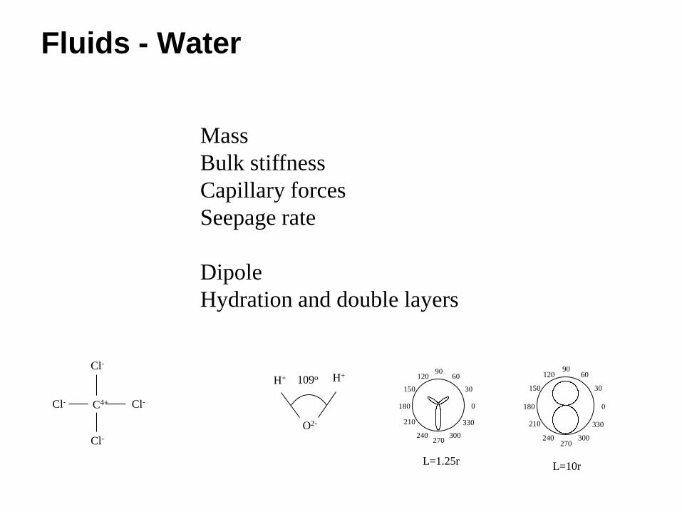
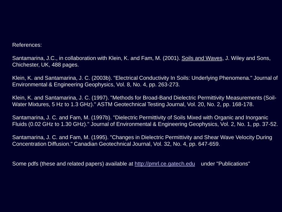
Fluids - Water

Mass

Bulk stiffness

Capillary forces

Seepage rate

Dipole

Hydration and double layers

O2-

H+ H+ 109o

0

30

60 90

120

150

180

210

240 270

300

330

L=1.25r

0

30

60 90

120

150

180

210

240 270

300

330

L=10r

Cl-

Cl-

Cl-

Cl-

C4+

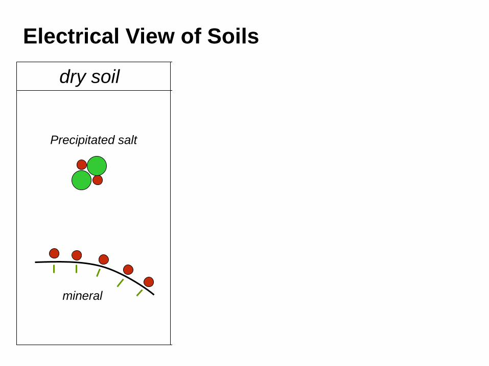
Electrical View of Soils

Precipitated salt

mineral

dry soil water

pore fluid

wet soil

double layer

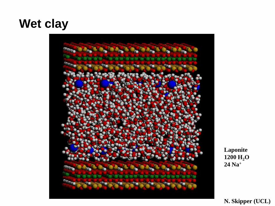
Wet clay

Laponite

1200 H2O

24 Na+

N. Skipper (UCL)

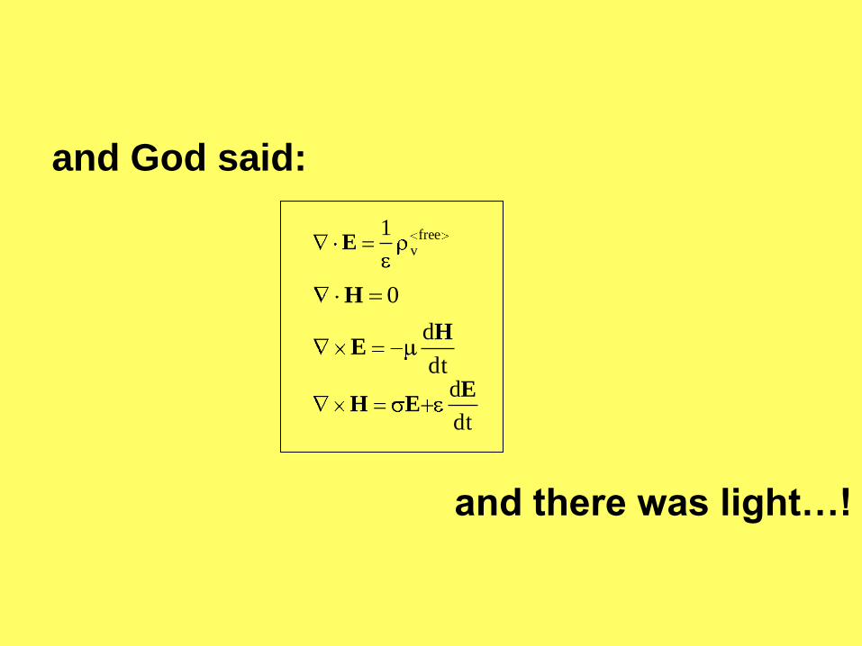
Electromagnetic Waves

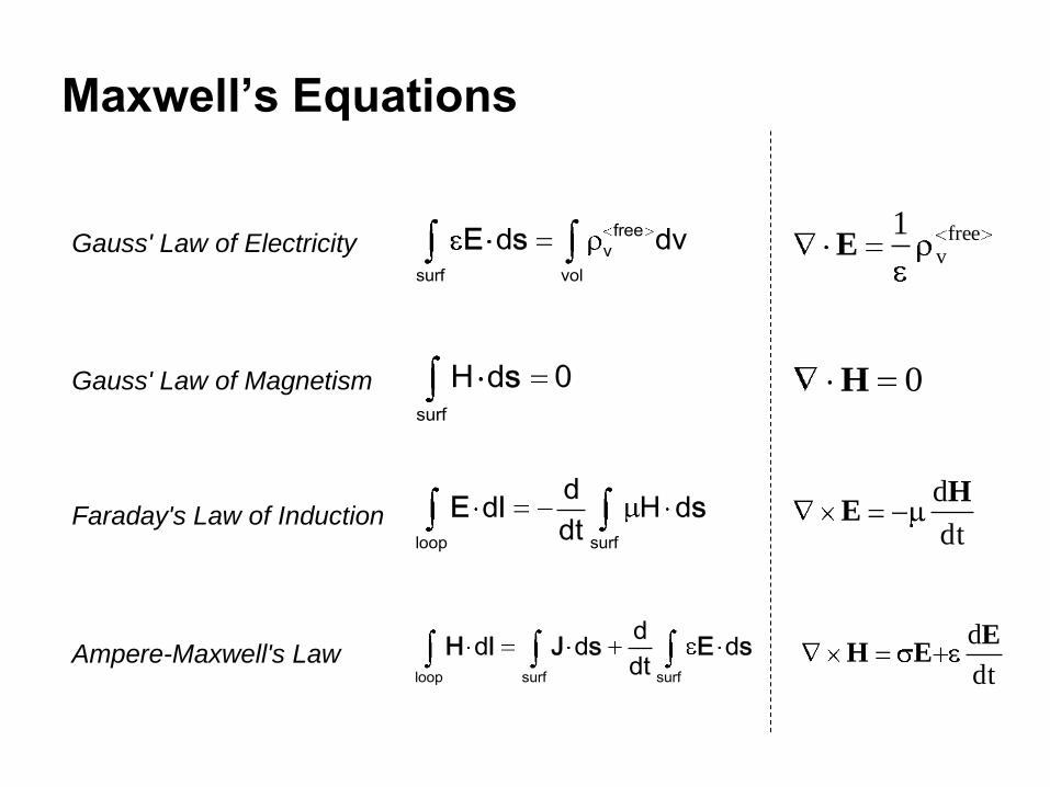
Maxwell’s Equations

free

v

surf vol

d dvE s freev

1E

surf

H d 0s 0H

loop surf

dd H d

dtE l s

dt

dHE

loop surf surf

dd d d

dtH l J s E s

dt

dEEH

Gauss' Law of Electricity

Gauss' Law of Magnetism

Faraday's Law of Induction

Ampere-Maxwell's Law

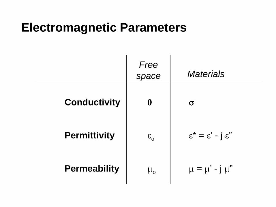
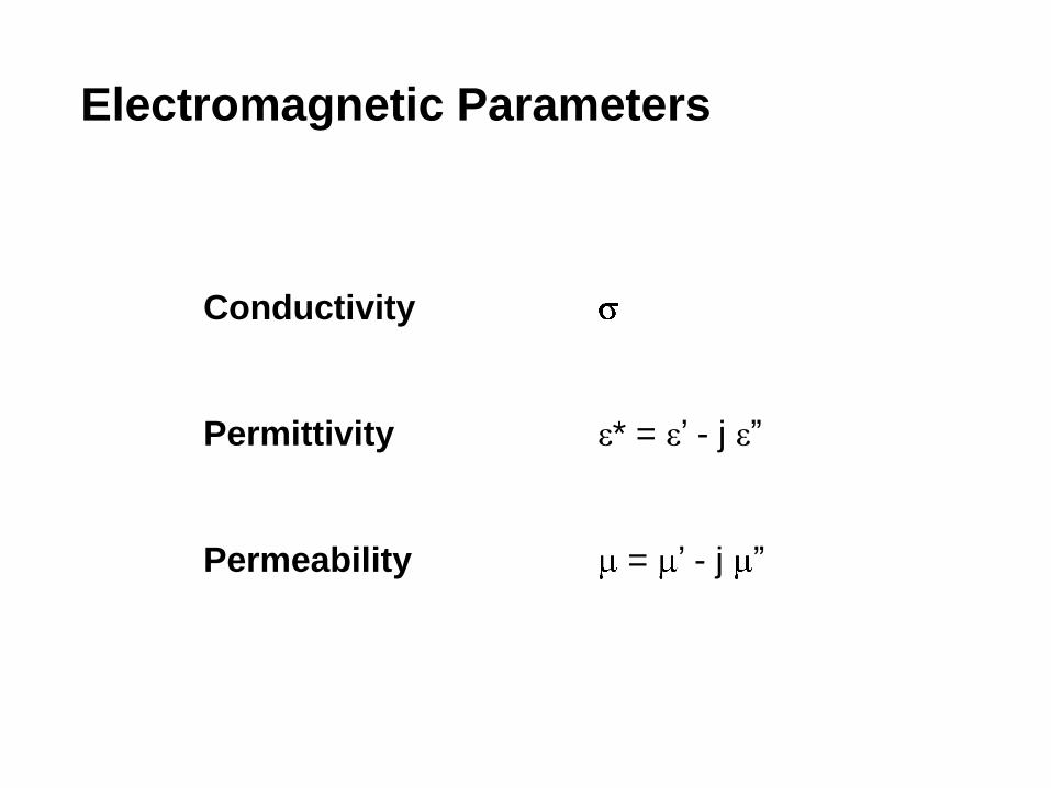
Conductivity 0

Permittivity εo ε* = ε’ - j ε”

Permeability o = ’ - j ”

Electromagnetic Parameters

Free

space Materials

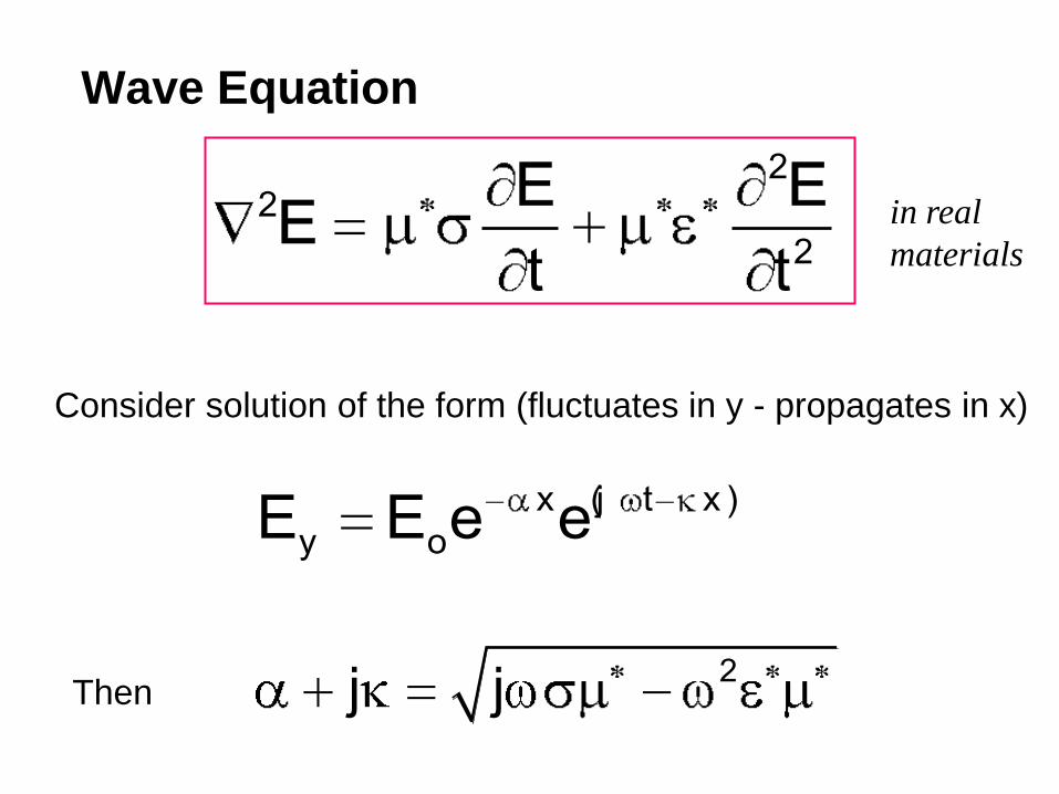
Wave Equation

22

2t t

E EE

x (j t x)

y oE E e e

Consider solution of the form (fluctuates in y - propagates in x)

Then 2j j

in real

materials

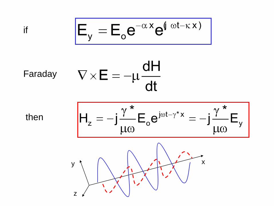
x (j t x)

y oE E e eif

dH

dtEFaraday

then j t * x

z o y

* *H j E e j E

x y

z

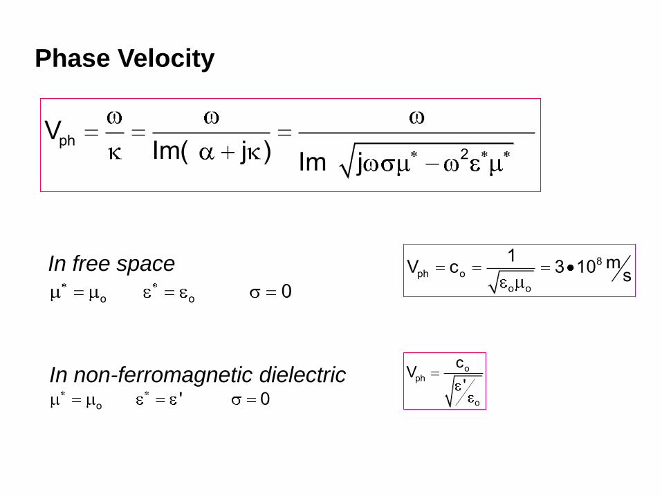
ph2

VIm( j ) Im j

Phase Velocity

In free space

o o 0

8

ph o

o o

1 mV c 3 10s

In non-ferromagnetic dielectric

o ' 0

oph

o

cV

'

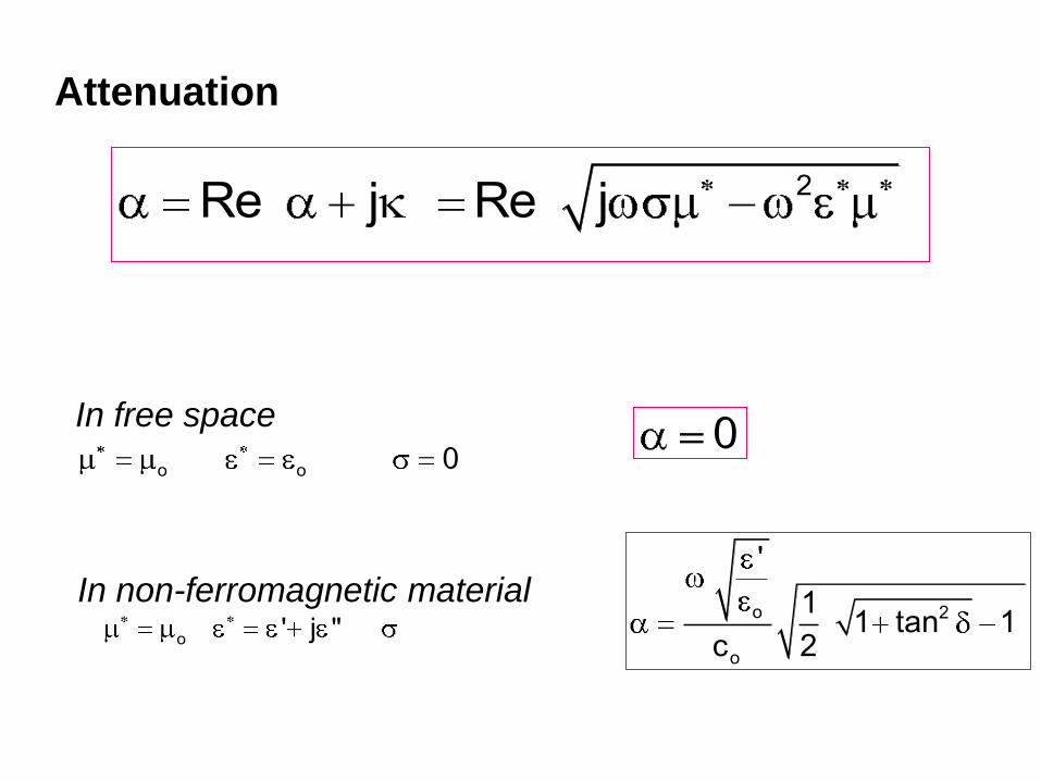
Attenuation

In free space

o o 00

In non-ferromagnetic material

o ' j "

2Re j Re j

o 2

o

'

11 tan 1

c 2

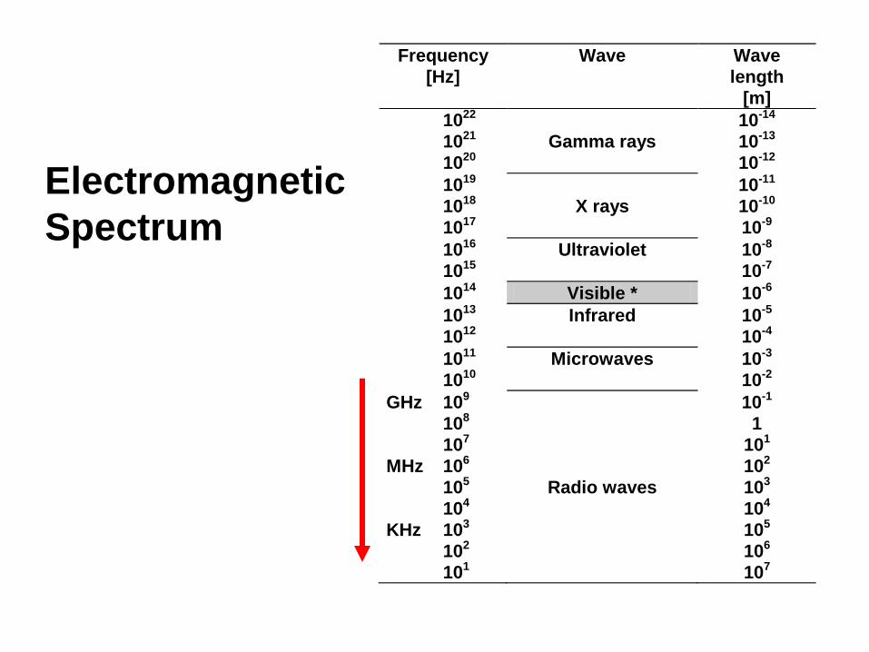
Frequency

[Hz]

Wave Wave

length

[m]

1022 10-14

1021 Gamma rays 10-13

1020 10-12

1019 10-11

1018 X rays 10-10

1017 10-9

1016 Ultraviolet 10-8

1015 10-7

1014 Visible * 10-6

1013 Infrared 10-5

1012 10-4

1011 Microwaves 10-3

1010 10-2

GHz 109 10-1

108 1

107 101

MHz 106 102

105 Radio waves 103

104 104

KHz 103 105

102 106

101 107

Electromagnetic

Spectrum

freev

1E

0H

dt

dHE

dt

dEEH

and God said:

and there was light…!

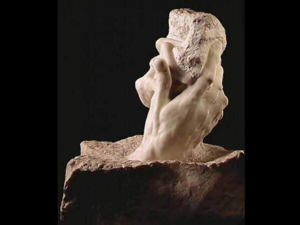
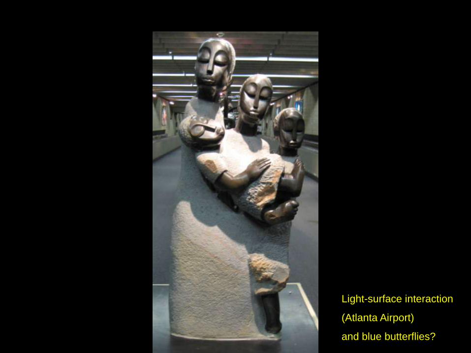
Light-surface interaction

(Atlanta Airport)

and blue butterflies?

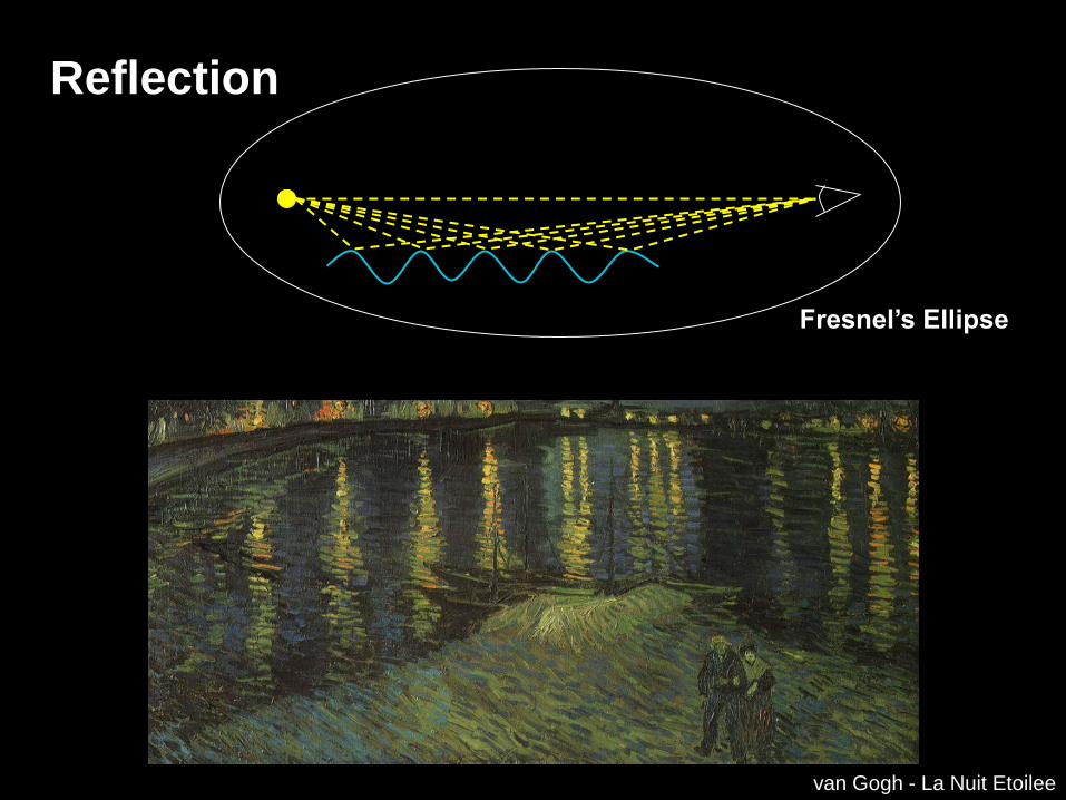
van Gogh - La Nuit Etoilee

Fresnel’s Ellipse

Reflection

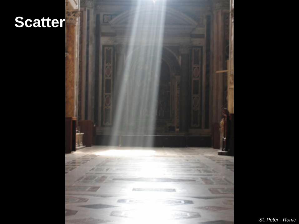
St. Peter - Rome

Scatter

Electromagnetic

Material Properties

Conductivity

Permittivity ε* = ε’ - j ε”

Permeability = ’ - j ”

Electromagnetic Parameters

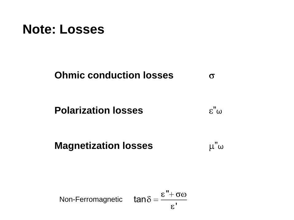
Ohmic conduction losses

Polarization losses ε”ω

Magnetization losses ”ω

Note: Losses

"tan

'Non-Ferromagnetic

Conductivity charges & mobility

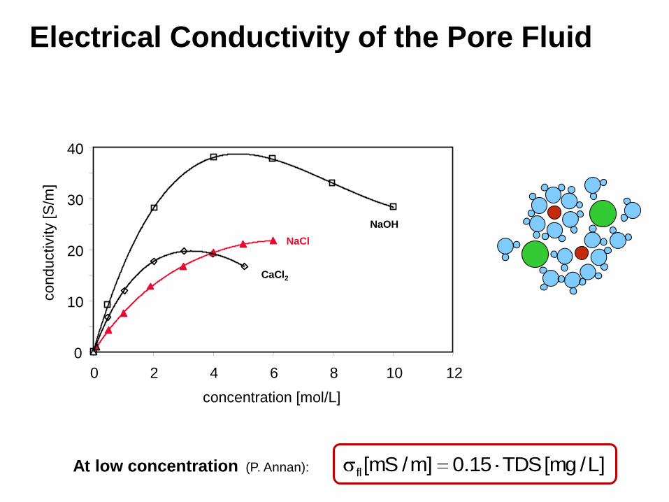
Electrical Conductivity of the Pore Fluid

0

10

20

30

40

0 2 4 6 8 10 12

concentration [mol/L]

conductivity [S

/m]

NaOH

NaCl

CaCl2

At low concentration (P. Annan): ]L/mg[TDS15.0]m/mS[fl

Archie’s Law?

elsoil n

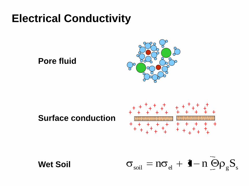
Electrical Conductivity

Surface conduction

Pore fluid

Wet Soil sgelsoilSn1n

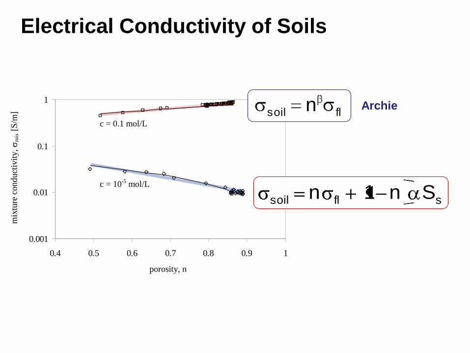
0.001

0.01

0.1

1

0.4 0.5 0.6 0.7 0.8 0.9 1

porosity, n

mix

ture

con

du

ctiv

ity

, m

ix [

S/m

]

c = 0.1 mol/L

c = 10-5 mol/L

Electrical Conductivity of Soils

Archie

sflsoil Sn1n

flsoil n

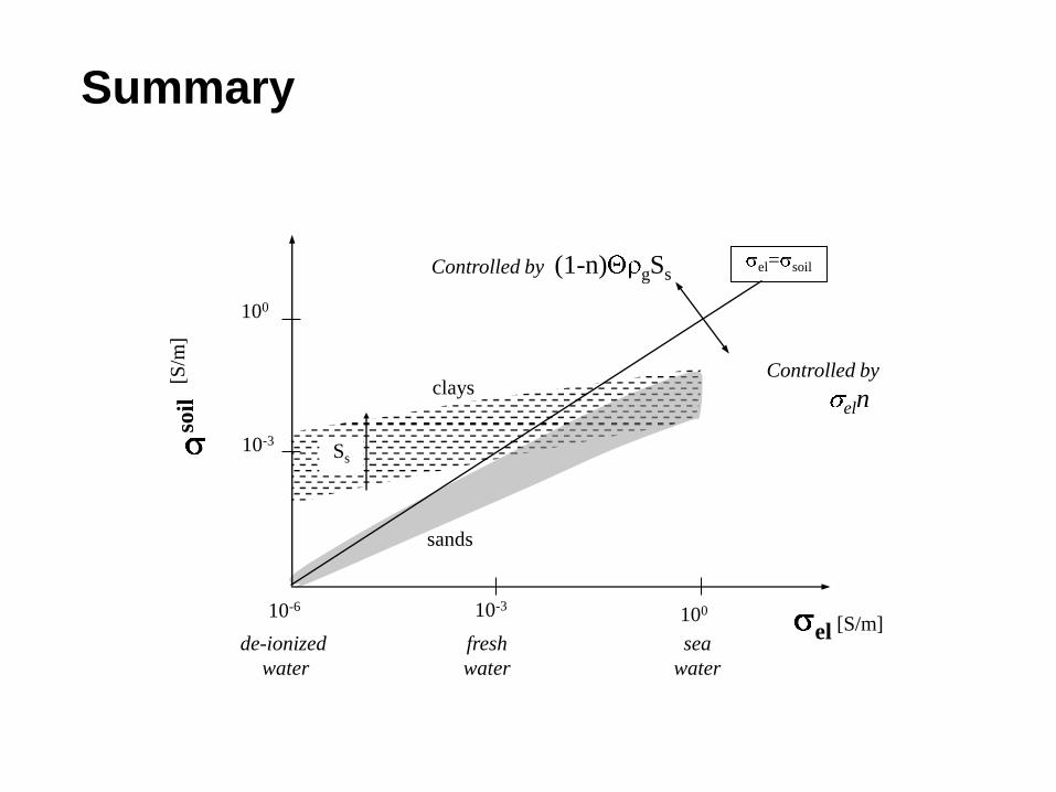
Summary

10-6 10-3 100

10-3

100

Controlled by

eln

Ss

clays

sands

soil

[

S/m

]

el [S/m]

el= soil

de-ionized

water

fresh

water

sea

water

Controlled by (1-n) gSs

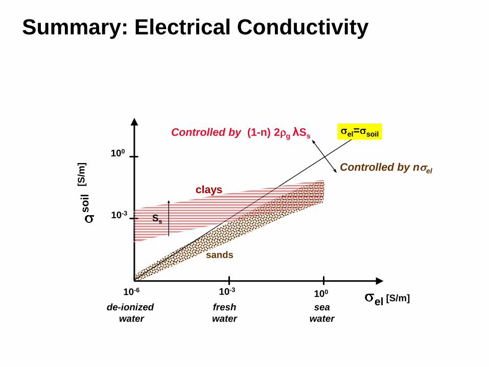
Summary: Electrical Conductivity

10-6 10-3 100

10-3

100

Controlled by n el

clays

sands

so

il

[S

/m]

el [S/m]

el= soil

de-ionized

water

fresh

water

sea

water

Controlled by (1-n) 2 g λSs

Ss

Permittivity Polarizability

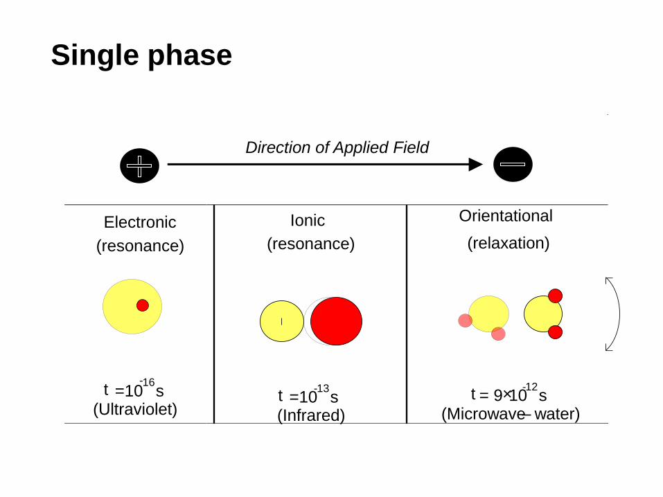
Single phase

Electronic

(resonance)

t =10 - 16

s (Ultraviolet)

Ionic

(resonance)

t =10

- 13 s

(Infrared)

Orientational

(relaxation)

t = 9 × 10 - 12

s (Microwave – water)

Direction of Applied Field

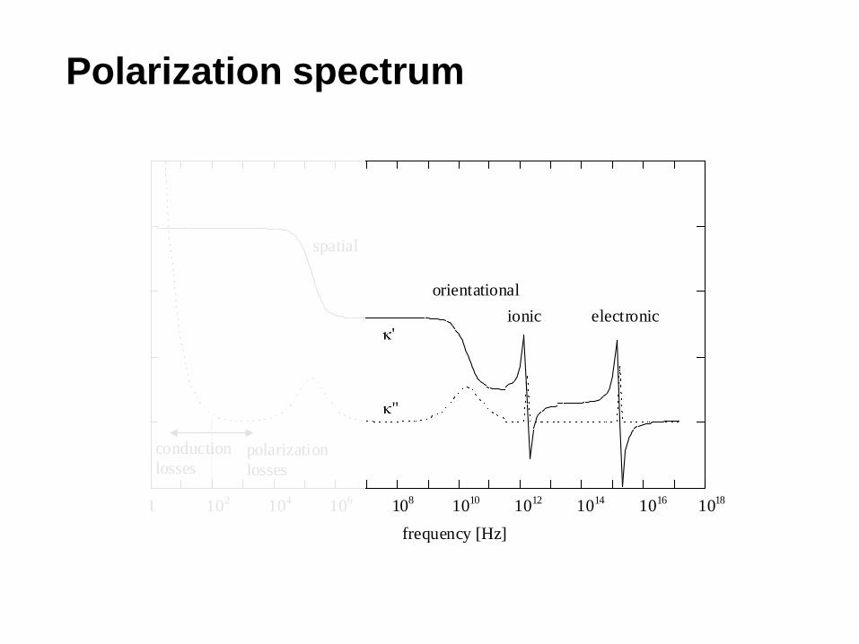
Polarization spectrum

1 10 100 1 103

1 104

1 105

1 106

1 107

1 108

1 109

1 1010

1 1011

1 1012

1 1013

1 1014

1 1015

1 1016

1 1017

1 1018

50

0

50

100

150

200

frequency [Hz]

"

'

spatial

orientational

ionic electronic

polarization

losses

conduction

losses

1 102 10

4 10

6 10

8 10

10 10

12 10

14 10

16 10

18

200

150

100

50

0

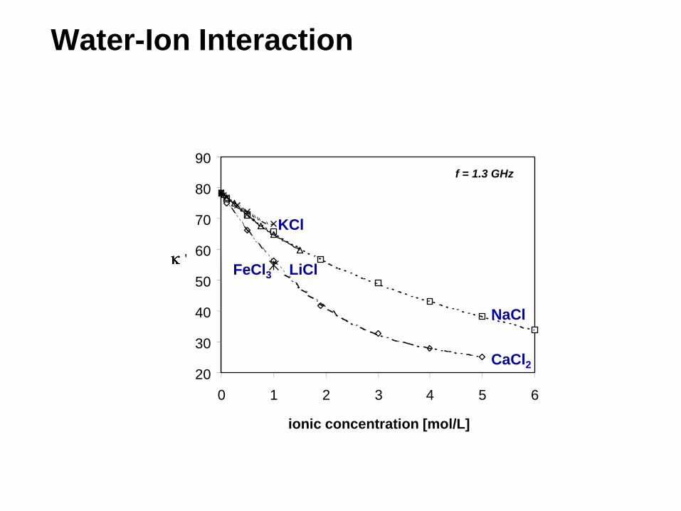
Water-Ion Interaction

20

30

40

50

60

70

80

90

0 1 2 3 4 5 6

'

ionic concentration [mol/L]

CaCl2

NaCl

KCl

LiCl FeCl3

f = 1.3 GHz

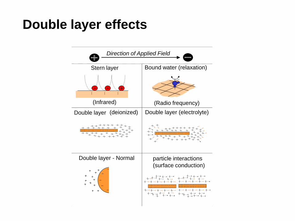
Double layer effects

Stern layer

(Infrared)

Bound water (relaxation) (Radio frequency)

Double layer (deionized)

Double layer (electrolyte)

Double layer - Normal particle interactions

(surface conduction)

Direction of Applied Field

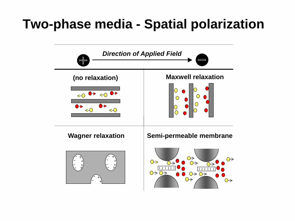
Two-phase media - Spatial polarization

(no relaxation) Maxwell relaxation

Wagner relaxation

Direction of Applied Field

Semi-permeable membrane

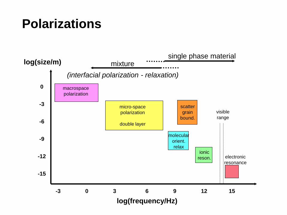
Polarizations

single phase material mixture

log(frequency/Hz)

-3 0 3 6 9 12 15

0

-3

-6

-9

-12

-15

visible

range

electronic

resonance

ionic

reson.

molecular

orient.

relax

scatter

grain

bound.

micro-space

polarization

double layer

macrospace

polarization

(interfacial polarization - relaxation)

log(size/m)

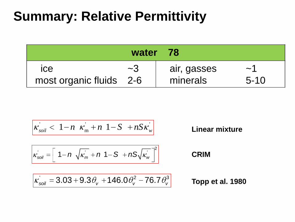
Summary: Relative Permittivity

water 78

ice ~3

most organic fluids 2-6

air, gasses ~1

minerals 5-10

2' ' '1 1soil m wn n S nS

' 2 33.03 9.3 146.0 76.7soil v v v Topp et al. 1980

CRIM

' ' '

m1 1soil wn n S nS Linear mixture

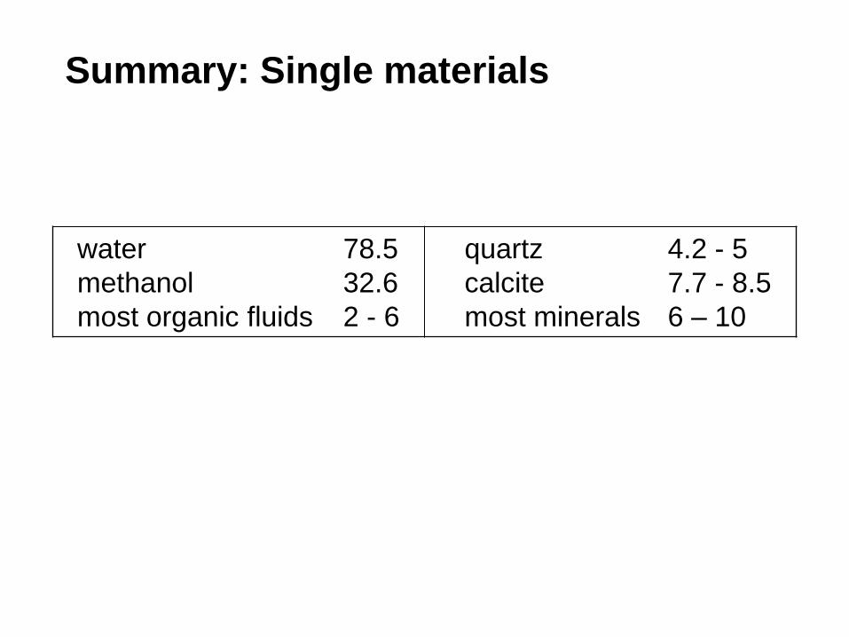
Summary: Single materials

water 78.5

methanol 32.6

most organic fluids 2 - 6

quartz 4.2 - 5

calcite 7.7 - 8.5

most minerals 6 – 10

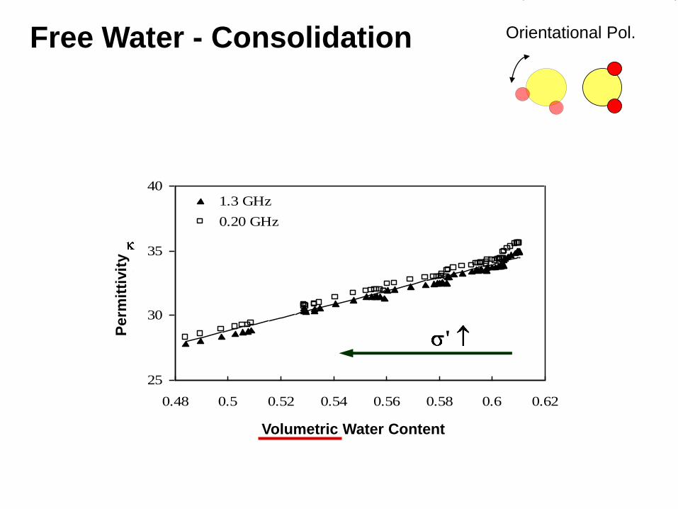
Free Water - Consolidation

Orientational Pol.

25

30

35

40

0.48 0.5 0.52 0.54 0.56 0.58 0.6 0.62

local volumetric water content

1.3 GHz

0.20 GHz

DeLoor

1.2

1.4

1.6

1.8

2

2.2

2.4

2.6

0.48 0.51 0.54 0.57 0.6 0.63

local volumetric water content

1.E+01

1.E+02

1.E+03

1.E+04

1.E+05

1.E+06

1.E+07

stre

ss [k

Pa]

'

"eff

(b)

(a)

stress

(Table 11.9)

Volumetric Water Content

Perm

itti

vit

y

'

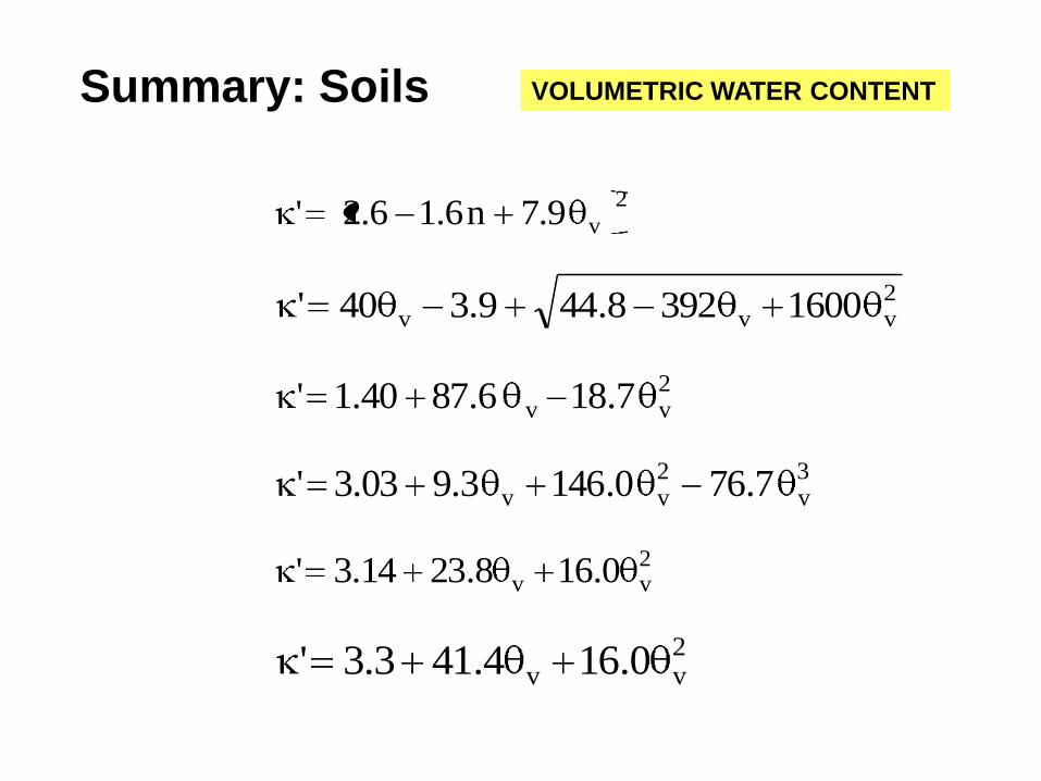
Summary: Soils

2vv 7.186.8740.1'

3v

2vv 7.760.1463.903.3'

2vv 0.164.413.3'

2vv 0.168.2314.3'

2vvv 16003928.449.340'

2

v9.7n6.16.2'

VOLUMETRIC WATER CONTENT

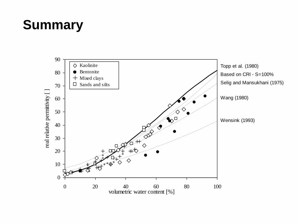
Summary

0

10

20

30

40

50

60

70

80

90

0 20 40 60 80 100volumetric water content [%]

real

rel

ativ

e per

mitt

ivity

[ ]

Kaolinite

Bentonite

Mixed clays

Sands and silts

Topp et al. (1980)

Selig and Mansukhani (1975)

Wang (1980)

Wensink (1993)

Based on CRI - S=100%

Permeability Magnetizability

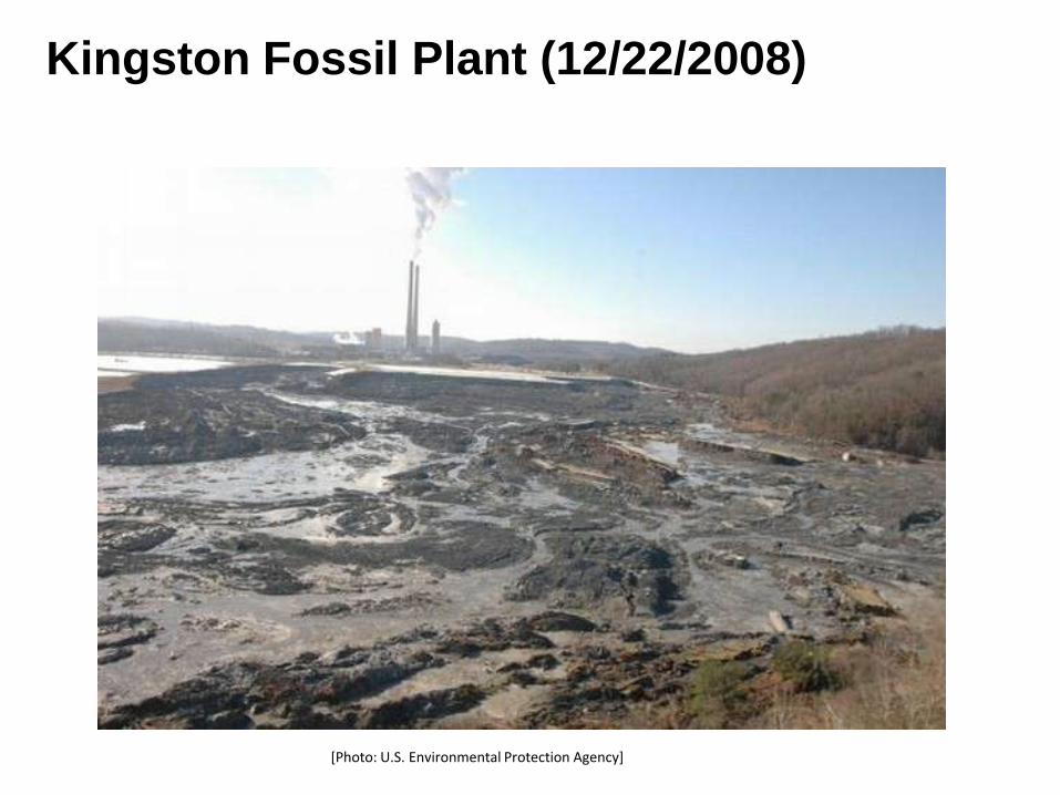
[Photo: U.S. Environmental Protection Agency]

Kingston Fossil Plant (12/22/2008)

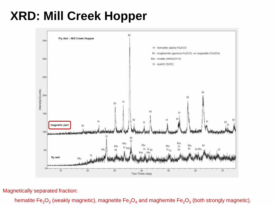
XRD: Mill Creek Hopper

Magnetically separated fraction:

hematite Fe2O3 (weakly magnetic), magnetite Fe3O4 and maghemite Fe2O3 (both strongly magnetic).

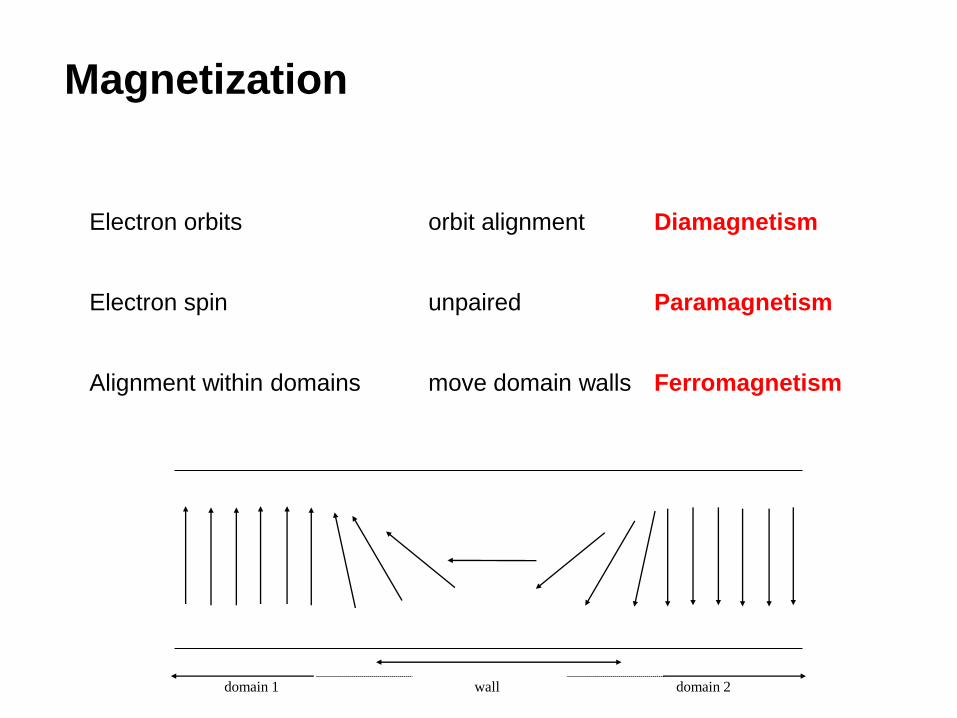
Magnetization

Electron orbits orbit alignment Diamagnetism

Electron spin unpaired Paramagnetism

Alignment within domains move domain walls Ferromagnetism

domain 1 domain 2 wall

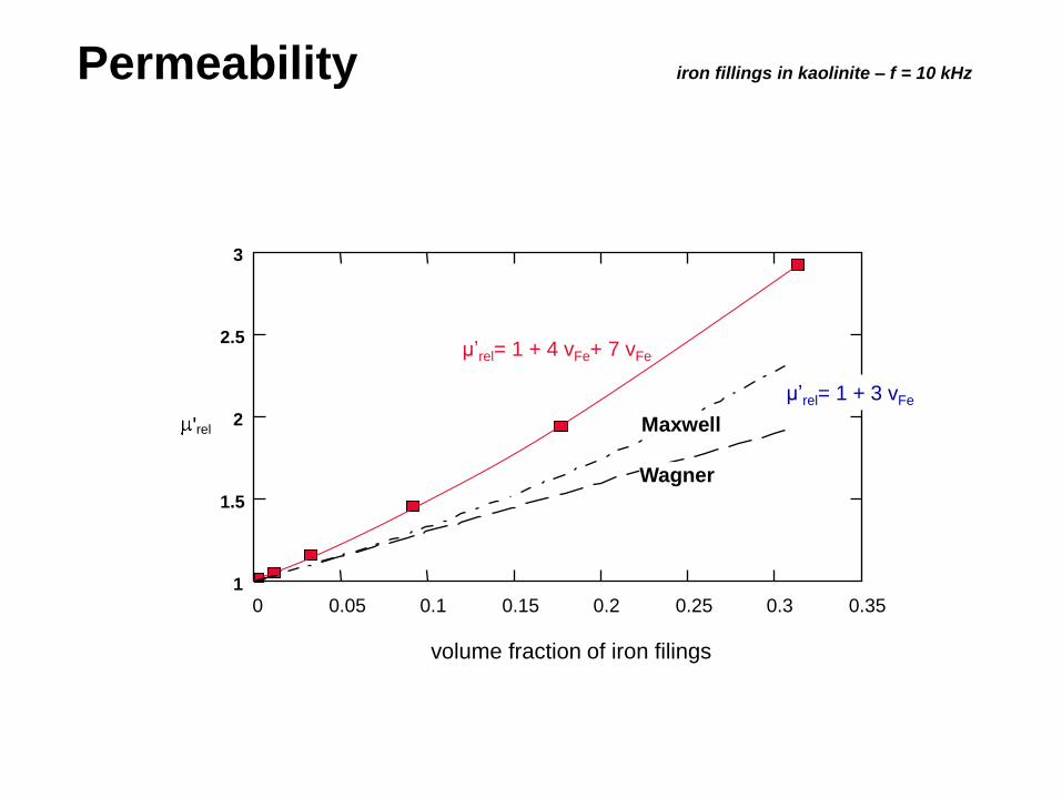
Permeability iron fillings in kaolinite – f = 10 kHz

' rel

volume fraction of iron filings

0 0.05 0.1 0.15 0.2 0.25 0.3 0.35 1

1.5

2

2.5

3

μ’rel= 1 + 4 vFe+ 7 vFe

μ’rel= 1 + 3 vFe

Maxwell

Wagner

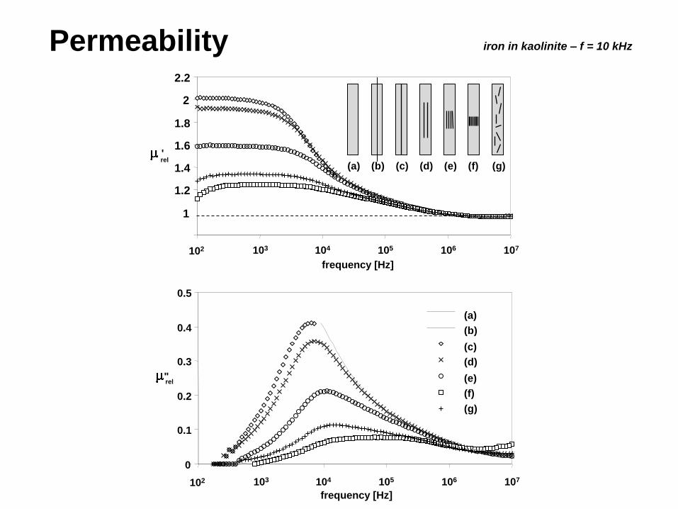
Permeability iron in kaolinite – f = 10 kHz

0

0.1

0.2

0.3

0.4

0.5

102 103 104 105 106 107

Series1

Series2

Series3

Series4

Series5

Series6

Series7

1

1.2

1.4

1.6

1.8

2

2.2

(a) (b) (c) (d) (e) (f) (g)

(a)

(b)

(c)

(d)

(e)

(f)

(g)

frequency [Hz]

frequency [Hz]

" rel

' rel

102 103 104 105 106 107

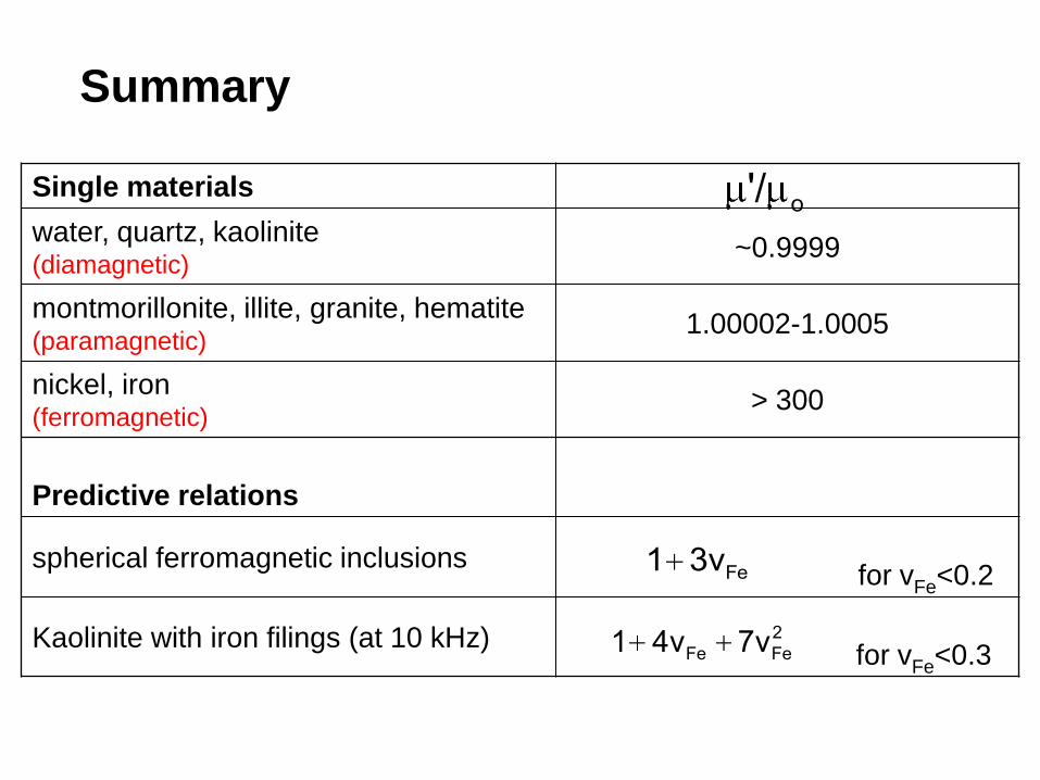
Summary

Fe1 3v

2

Fe Fe1 4v 7v

Single materials

water, quartz, kaolinite (diamagnetic)

~0.9999

montmorillonite, illite, granite, hematite (paramagnetic)

1.00002-1.0005

nickel, iron (ferromagnetic)

> 300

Predictive relations

spherical ferromagnetic inclusions

for vFe<0.2

Kaolinite with iron filings (at 10 kHz)

for vFe<0.3

o'/

Measurement

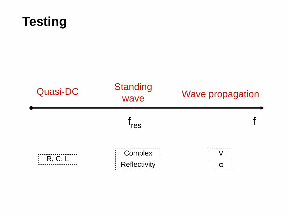
Testing

f

Quasi-DC Wave propagation Standing

wave

fres

R, C, L Complex

Reflectivity

V

α

Quasi-static

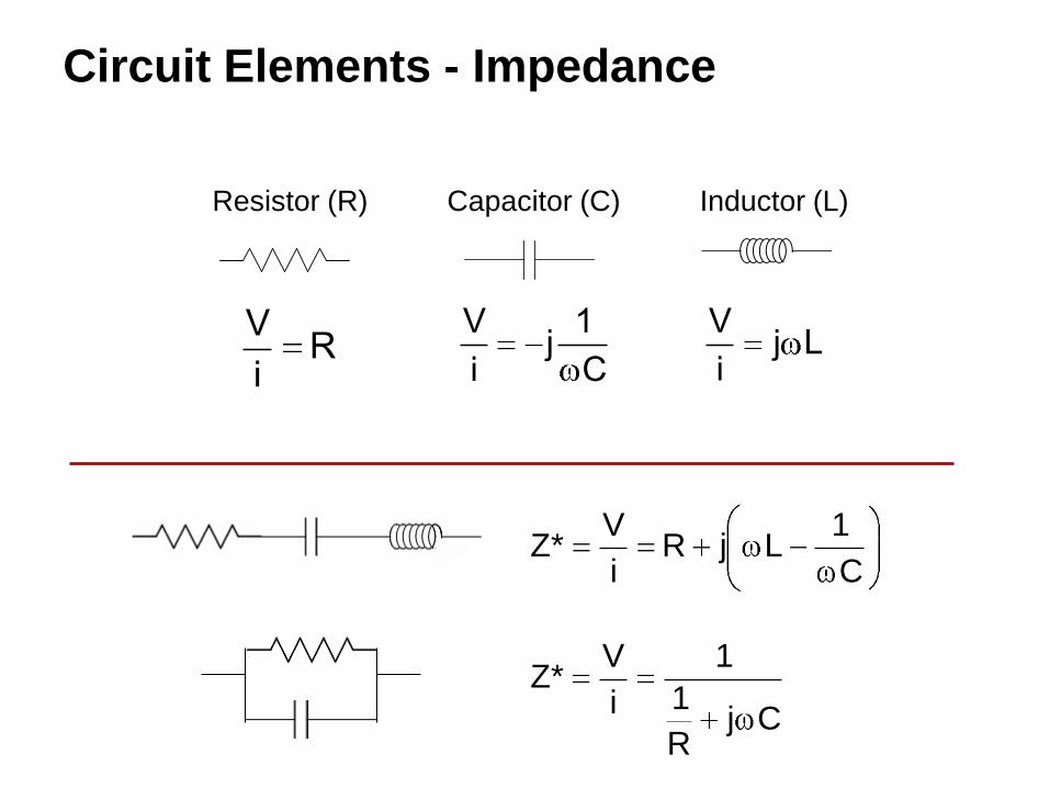
VR

i

Vj L

i

V 1j

i C

Resistor (R) Inductor (L) Capacitor (C)

CjR

1

1

i

V*Z

C

1LjR

i

V*Z

Circuit Elements - Impedance

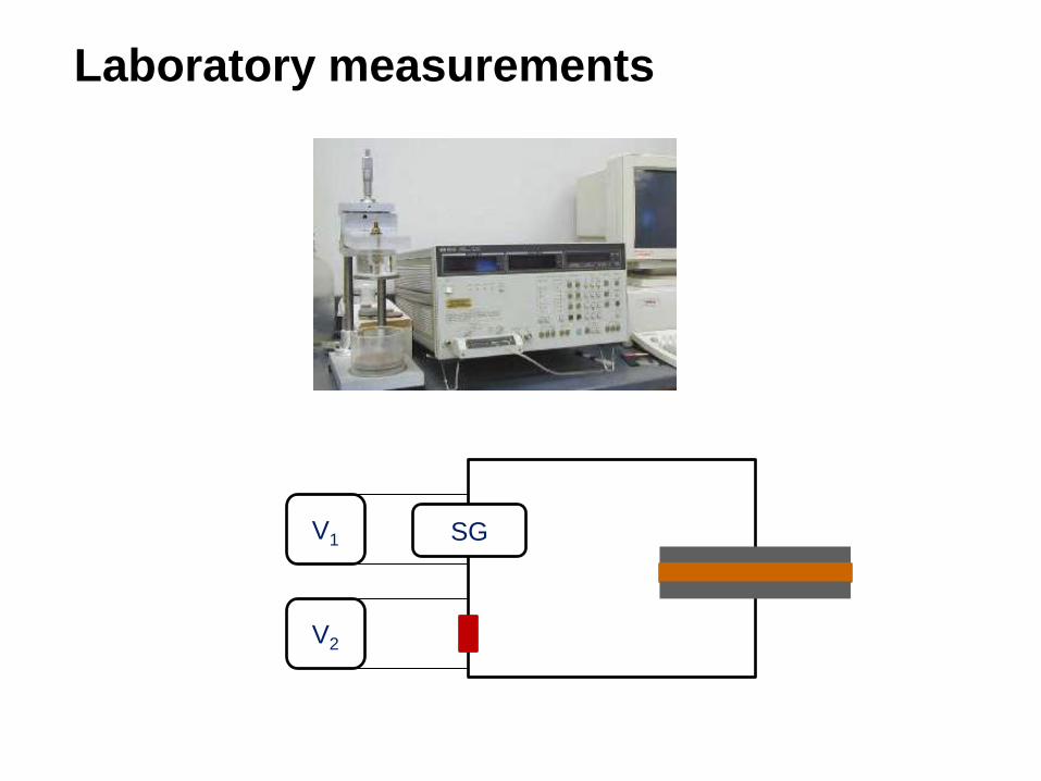
Laboratory measurements

SG V1

V2

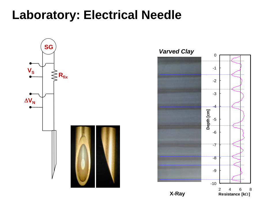
-10

-9

-8

-7

-6

-5

-4

-3

-2

-1

0

2 4 6 8

Resistance [k ]

Dep

th [

cm

]

X-Ray

Varved Clay

Laboratory: Electrical Needle

Rfix

VN

VS

SG

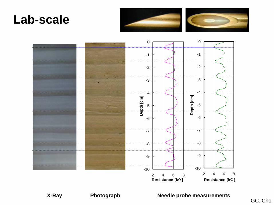
Photograph X-Ray

Lab-scale

-10

-9

-8

-7

-6

-5

-4

-3

-2

-1

0

2 4 6 8

Resistance [k ]

Dep

th [

cm

]

-10

-9

-8

-7

-6

-5

-4

-3

-2

-1

0

2 4 6 8

Resistance [k ]

Dep

th [

cm

]

Needle probe measurements GC. Cho

1 2

3

16

15

14

13

12

11

10

9

8

7

6

5

4

1 2

3

16

15

14

13

12

11

10

9

8

7

6

5

4

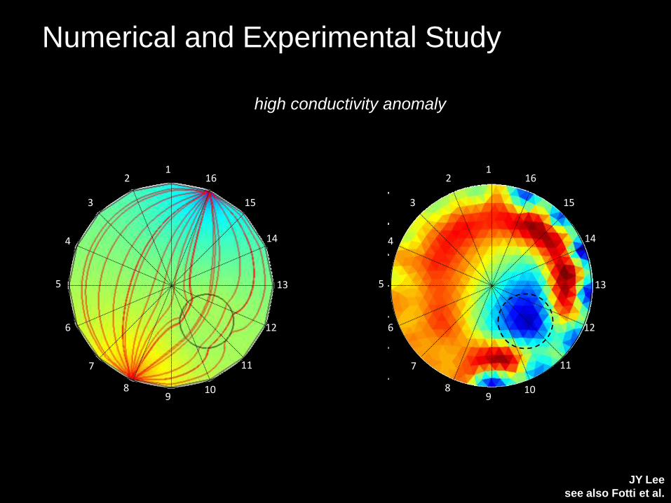
Numerical and Experimental Study

high conductivity anomaly

JY Lee

see also Fotti et al.

WAVE PROPAGATION

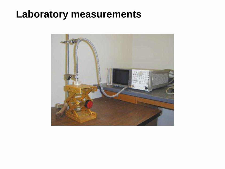
Laboratory measurements

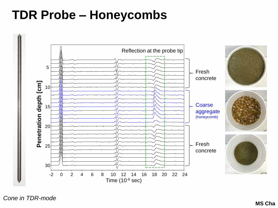
TDR Probe – Honeycombs

Coarse

aggregate (honeycomb)

Fresh

concrete

Fresh

concrete

Time (10-9 sec) -2 0 2 4 6 8 10 12 14 16 18 20 22 24

Reflection at the probe tip

Pen

etr

ati

on

dep

th [

cm

]

5

20

25

30

10

15

Cone in TDR-mode MS Cha

Field Devices

Typical Data

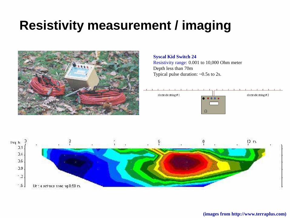
Syscal Kid Switch 24

Resistivity range: 0.001 to 10,000 Ohm meter

Depth less than 70m

Typical pulse duration: ~0.5s to 2s.

Resistivity measurement / imaging

(images from http://www.terraplus.com)

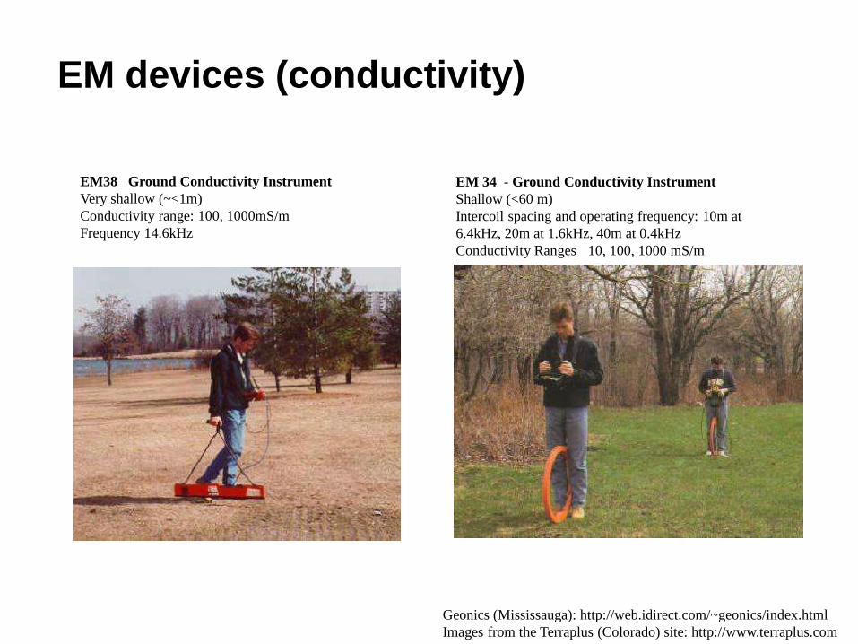
EM38 Ground Conductivity Instrument

Very shallow (~<1m)

Conductivity range: 100, 1000mS/m

Frequency 14.6kHz

Geonics (Mississauga): http://web.idirect.com/~geonics/index.html

Images from the Terraplus (Colorado) site: http://www.terraplus.com

EM 34 - Ground Conductivity Instrument

Shallow (<60 m)

Intercoil spacing and operating frequency: 10m at

6.4kHz, 20m at 1.6kHz, 40m at 0.4kHz

Conductivity Ranges 10, 100, 1000 mS/m

EM devices (conductivity)

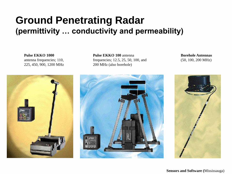
Sensors and Software (Mississauga)

Borehole Antennas

(50, 100, 200 MHz)

Pulse EKKO 100 antenna

frequencies; 12.5, 25, 50, 100, and

200 MHz (also borehole)

Pulse EKKO 1000

antenna frequencies; 110,

225, 450, 900, 1200 MHz

Ground Penetrating Radar (permittivity … conductivity and permeability)

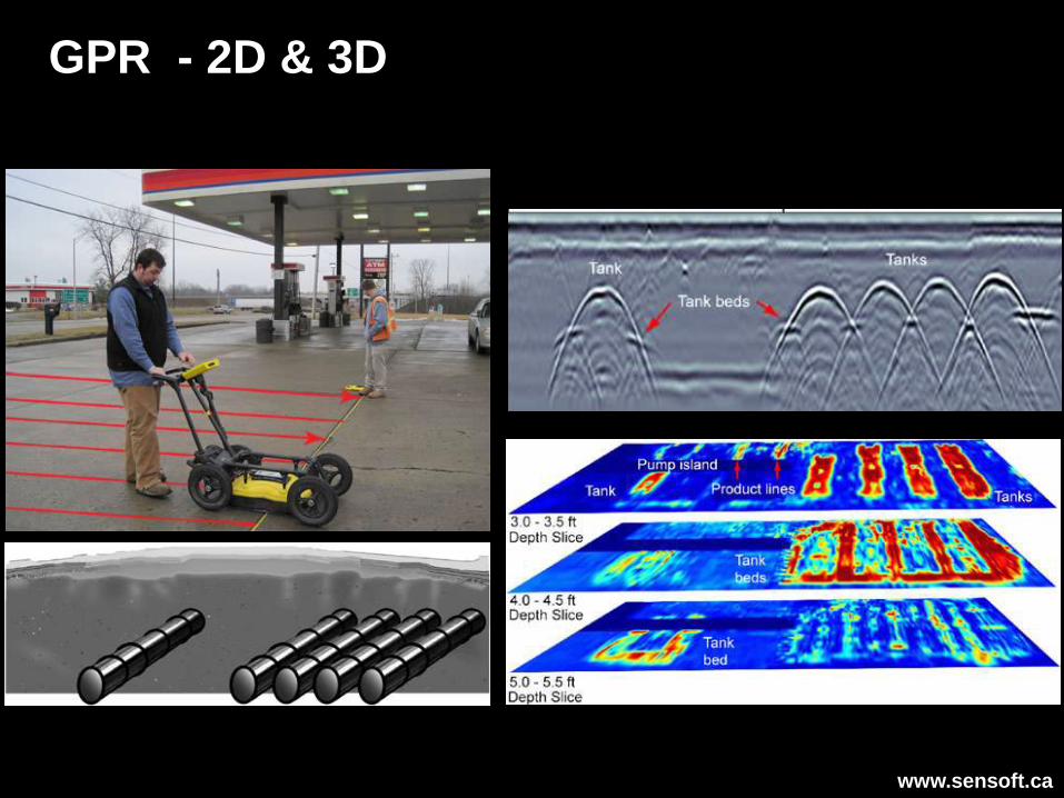
GPR - 2D & 3D

www.sensoft.ca

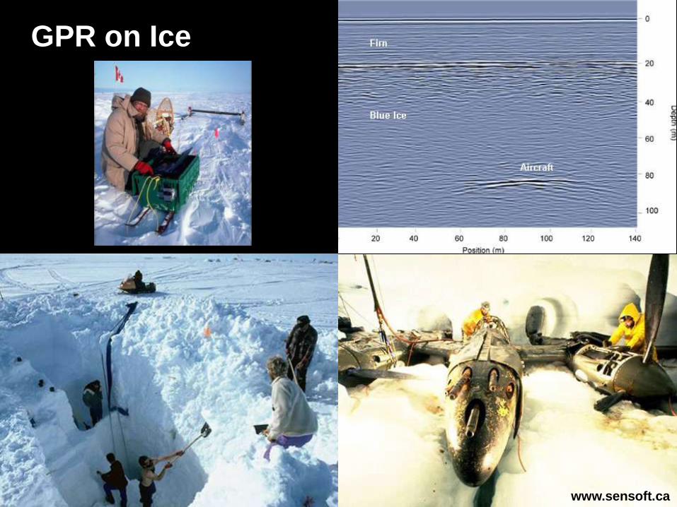
GPR on Ice

www.sensoft.ca

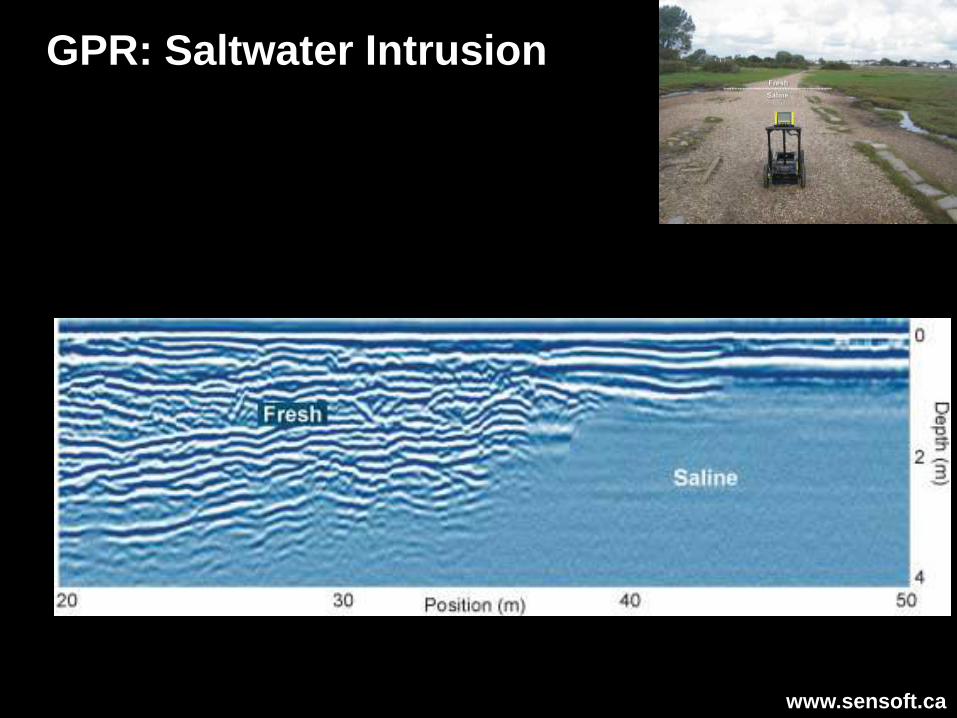
www.sensoft.ca

GPR: Saltwater Intrusion

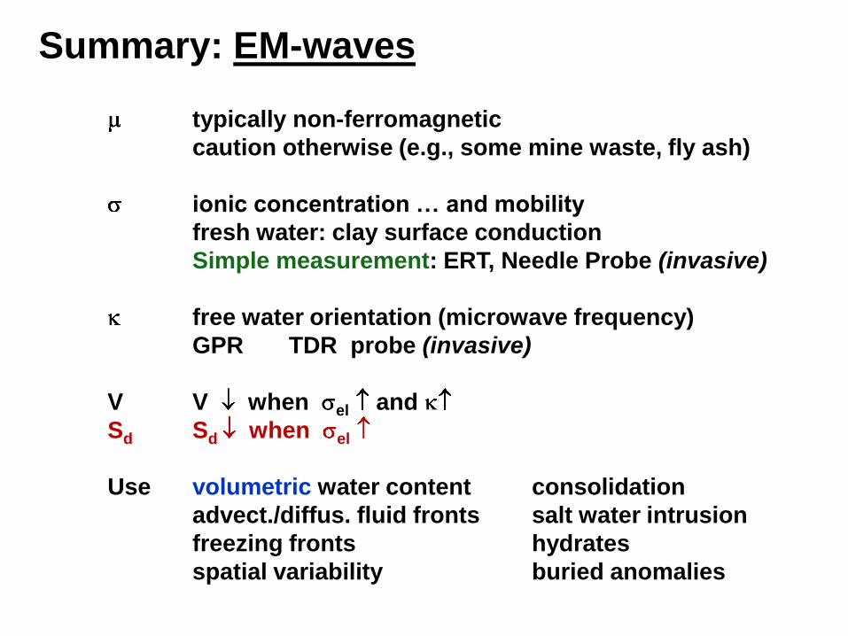
Summary: EM-waves

typically non-ferromagnetic

caution otherwise (e.g., some mine waste, fly ash)

ionic concentration … and mobility

fresh water: clay surface conduction

Simple measurement: ERT, Needle Probe (invasive)

free water orientation (microwave frequency)

GPR TDR probe (invasive)

V V when el and

Sd Sd when el

Use volumetric water content consolidation

advect./diffus. fluid fronts salt water intrusion

freezing fronts hydrates

spatial variability buried anomalies