Embed Size (px)
Citation preview
Electromagnetic Theory Page 1 Lecture 1
DIV, GRAD, CURL AND ALL THAT……… Scalar Functions e.g. Temperature T (x, y, z)
Function of (x, y, z) Vector Functions:
( ) ( ) ( ) ( ), , , , , , , ,
and are scalar functionsx y z
x y z
x y z F x y z F x y z F x y z
F F F
= + +F i j k
Specifies magnitude and direction e.g. Velocity of a fluid
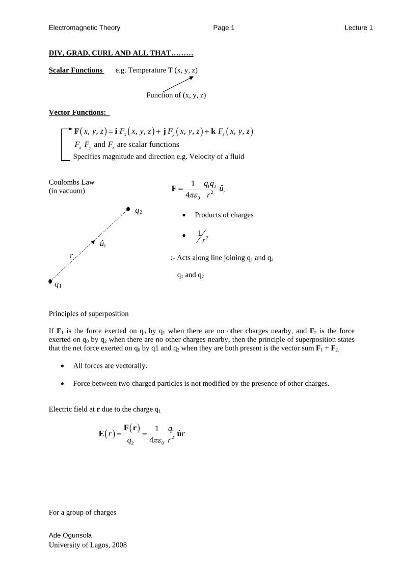
Coulombs Law 1 2
20
1 ˆ4 r
q q urπε
=F
• Products of charges
• 2
1r
:- Acts along line joining q1 and q2
q1 and q2
(in vacuum)
q1
ûr
q2
r
Principles of superposition If F1 is the force exerted on q0 by q1 when there are no other charges nearby, and F2 is the force exerted on q0 by q2 when there are no other charges nearby, then the principle of superposition states that the net force exerted on q0 by q1 and q2 when they are both present is the vector sum F1 + F2.
• All forces are vectorally.
• Force between two charged particles is not modified by the presence of other charges. Electric field at r due to the charge q1
( ) ( ) 12
2 0
1 ˆ4
qr rq rπε
= =F r
E u
For a group of charges
Ade Ogunsola University of Lagos, 2008
Electromagnetic Theory Page 2 Lecture 1
( ) 0 12
10
1 ˆ4
N
ll l
q q rπε =
=−
∑F r urr r
Force on q0 at i y k= + +r x j z
due to charges at lq lr
( ) 1210
1 ˆ ,4
Nl
l l
q u rπε =
=−
∑E r rr r
Electrostatic field at
x y z= + +r i j k due to charges at lq lr
( ) ( )1
1 1
210
ˆ ,14 V
r r dvρ
πε=
−∫∫∫
r uE r
r r
1
r
r1
( )1ρ r
∂v
V1
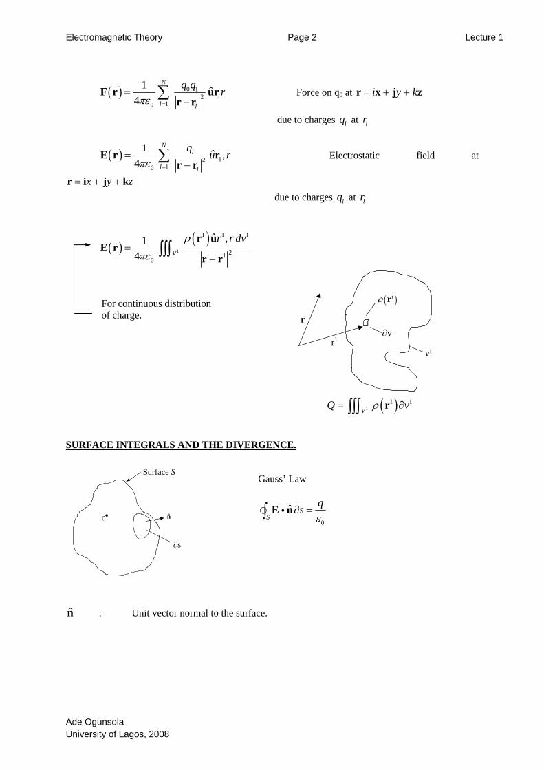
For continuous distribution of charge.
1 1Q vρ= ∂r SURFACE INTEGRALS AND THE DIVERGENCE.
q n
∂s
Surface S
Gauss’ Law
ˆS
qsε
∂ =∫ E ni
n : Unit vector normal to the surface.
Ade Ogunsola University of Lagos, 2008
( )1V∫∫∫
0
Electromagnetic Theory Page 3 Lecture 1
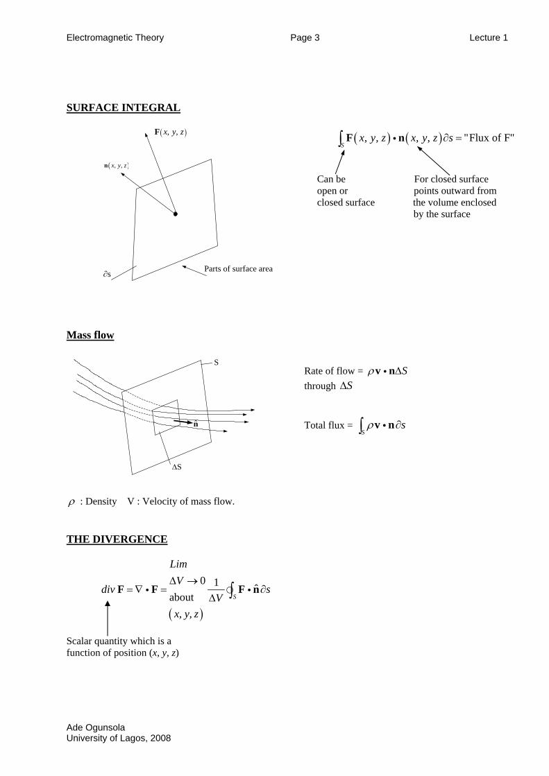
SURFACE INTEGRAL
( ), ,x y zF
( ), ,x y zn
∂s Parts of surface area
( ) ( ), , , , "Flux of F"S
x y z x y z s∂ =∫ F ni
Can be For closed surface open or points outward from closed surface the volume enclosed by the surface
Mass flow
S
T
Sf
AU
S∆
n
Rate of flow = Sρ ∆v ni through S∆ Total flux =
Ssρ ∂∫ v ni
ρ : Density V : Velocity of mass flow.
HE DIVERGENCE
( )
0 1 ˆabout S
LimV
div sV
x, y, z
∆ →=∇ = ∂
∆ ∫F F F ni i
calar quantity which is a unction of position (x, y, z)
de Ogunsola niversity of Lagos, 2008
Electromagnetic Theory Page 4 Lecture 1
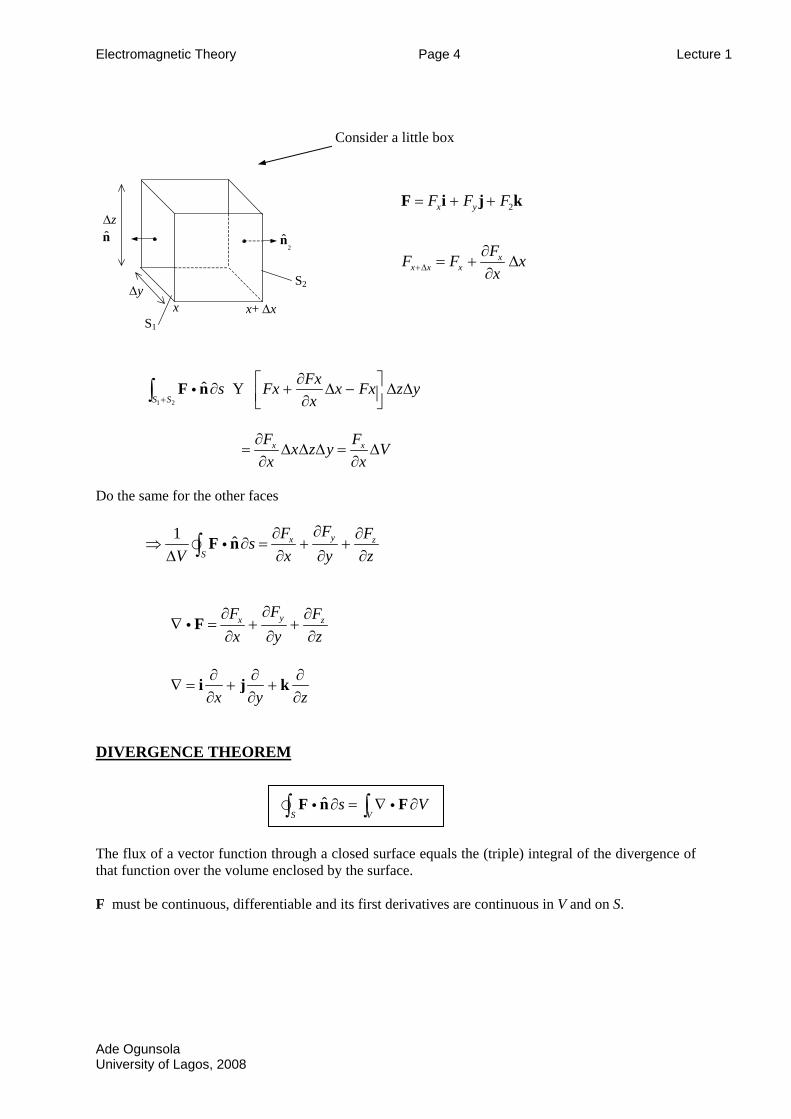
Consider a little box
ˆz∆
n
y∆
S1
x x+ ∆x
2n
S2
2x yF F F= + +F i j k
1 2
ˆS S
Fxs Fx x Fxx+
∂⎡ ⎤∂ + ∆ − ∆⎢ ⎥∂⎣ ⎦∫ F ni Y
x xF Fx z y V
x x∂
= ∆ ∆ ∆ = ∆∂ ∂
Do the same for the other faces
1 ˆ yx zS
FF FsV x y
∂∂z
∂⇒ ∂ = + +
∆ ∂ ∂∫ F ni∂
yx zFF F
x y z∂∂ ∂
∇ = + +∂ ∂ ∂
Fi
x y z∂ ∂ ∂+ +
∂ ∂ ∂i∇ = j k
DIVERGENCE THEOREM
ˆS V
s∂ = ∇∫ ∫F ni The flux of a vector function through a closed surthat function over the volume enclosed by the surf F must be continuous, differentiable and its first d
Ade Ogunsola University of Lagos, 2008
xx x x
FF Fx+∆ x∂
= + ∆∂
z y∆
V∂Fi
face equals the (triple) integral of the divergence of ace.
erivatives are continuous in V and on S.
Electromagnetic Theory Page 5 Lecture 1
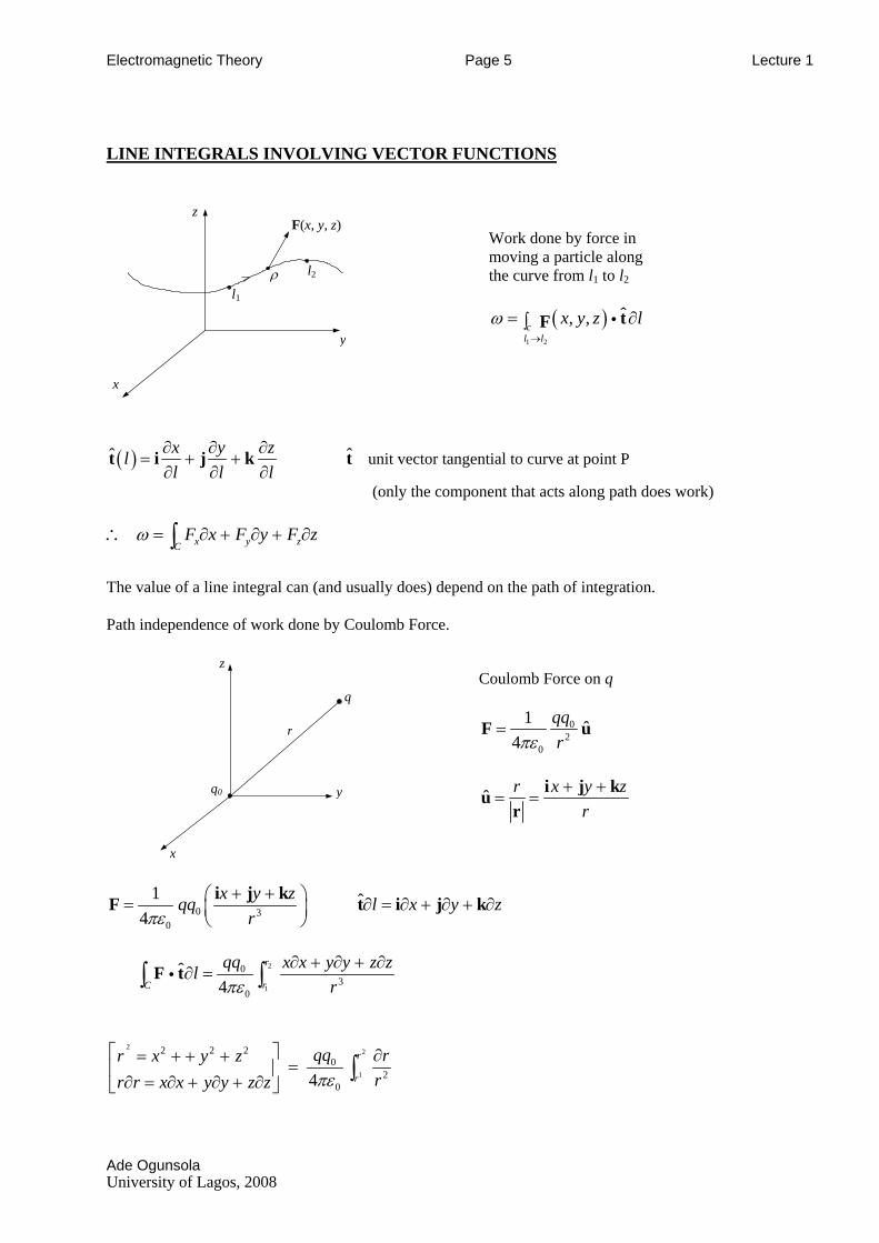
LINE INTEGRALS INVOLVING VECTOR FUNCTIONS
x
y
z F(x, y, z)
l2 ρ l1
Work done by force in moving a particle along the curve from l1 to l2
( )1 2
ˆ, ,cl l
x y z lω→
= ∂∫ tF i
( )ˆ x y zll l l
∂ ∂ ∂= + +
∂ ∂ ∂t i j k t unit vector tangential to curve at point P
(only the component that acts along path does work) ∴ x y zC
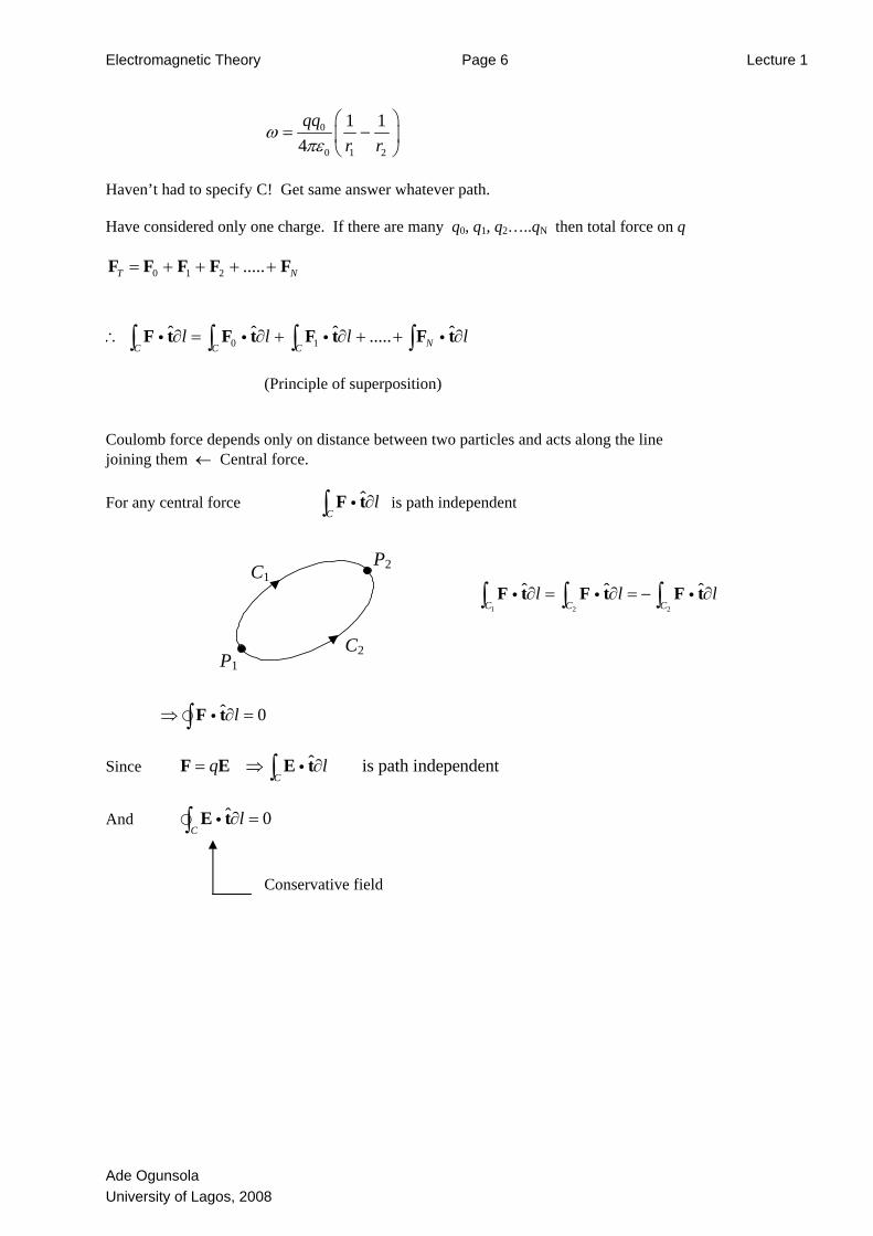
F x F y F zω = ∂ + ∂ + ∂∫ The value of a line integral can (and usually does) depend on the path of integration. Path independence of work done by Coulomb Force.
q
z
r
q0 y
x
Coulomb Force on q
02
0
1 ˆ4
qqrπε
=F u
ˆ r x yr
z+ += =
i j kur
0 30
1 ˆ4
x y zqq l x y zrπε
+ +⎛ ⎞= ∂ =⎜ ⎟⎝ ⎠
i j kF t ∂ + ∂ + ∂i j k
2
1
03
0
ˆ4
r
C r
qq x x y y z zlrπε
∂ + ∂ + ∂∂ =∫ ∫F ti
22
1
2 2 20
204
r
r
qq rr x y zrr r x x y y z z πε
⎡ ⎤ ∂= + + + =⎢ ⎥∂ = ∂ + ∂ + ∂⎣ ⎦
∫
Ade Ogunsola University of Lagos, 2008
Electromagnetic Theory Page 6 Lecture 1
0
0 1 2
1 14qq
r rω
πε⎛ ⎞
= −⎜ ⎟⎝ ⎠
Haven’t had to specify C! Get same answer whatever path. Have considered only one charge. If there are many q0, q1, q2…..qN then total force on q
0 1 2
0 1
.....
ˆ ˆ ˆ .....
T N
NC C Cl l l
= + + + +
ˆ l∴ ∂ = ∂ + ∂ + + ∂∫ ∫ ∫ ∫
F F F F F
F t F t F t F ti i i i
(Principle of superposition)
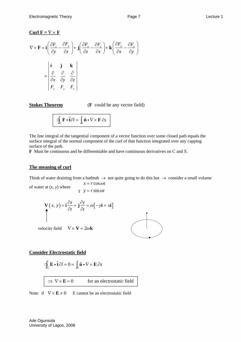
Coulomb force depends only on distance between two particles and acts along the line joining them ← Central force. For any central force ˆ
Cl∂∫ F ti is path independent
C1
C2 P1
P2
ˆ 0l⇒ ∂ =∫ F ti
Since F E ˆ is path indepen
Cq l= ⇒ ∂∫ E ti
ˆ lˆ ˆl l∂ = ∂ = −F t F t F ti i ∂i
And ˆ 0
Cl∂ =∫ E ti
Conservative field
Ade OgunsolaUniversity of Lagos, 2008
dent
1 2 2C C C∫ ∫ ∫
Electromagnetic Theory Page 7 Lecture 1
Curl F = ∇ × F
y yx xz zF FF FF F
y z z x x y∂ ∂⎛ ⎞ ⎛∂ ∂∂ ∂⎛ ⎞∇ × = − + − + −⎜ ⎟ ⎜⎜ ⎟∂ ∂ ∂ ∂ ∂ ∂⎝ ⎠⎝ ⎠ ⎝
F i j k⎞⎟⎠
x y z
x y zF F F
∂ ∂ ∂=
∂ ∂ ∂
i j k
Stokes Theorem (F could be any vector field)
ˆ ˆl s∂ = ∇ ×F t n Fi i ∂ The line integsurface integrsurface of the F Must be co The meanin Think of wate
of water at (x,
(xV
Consider El
C∫ E
⇒ Note: if ∇×
Ade OgunsolaUniversity of L
C S∫ ∫
ral of the tangential component of a vector function over some closed path equals the al of the normal component of the curl of that function integrated over any capping path. ntinuous and be differentiable and have continuous derivatives on C and S.
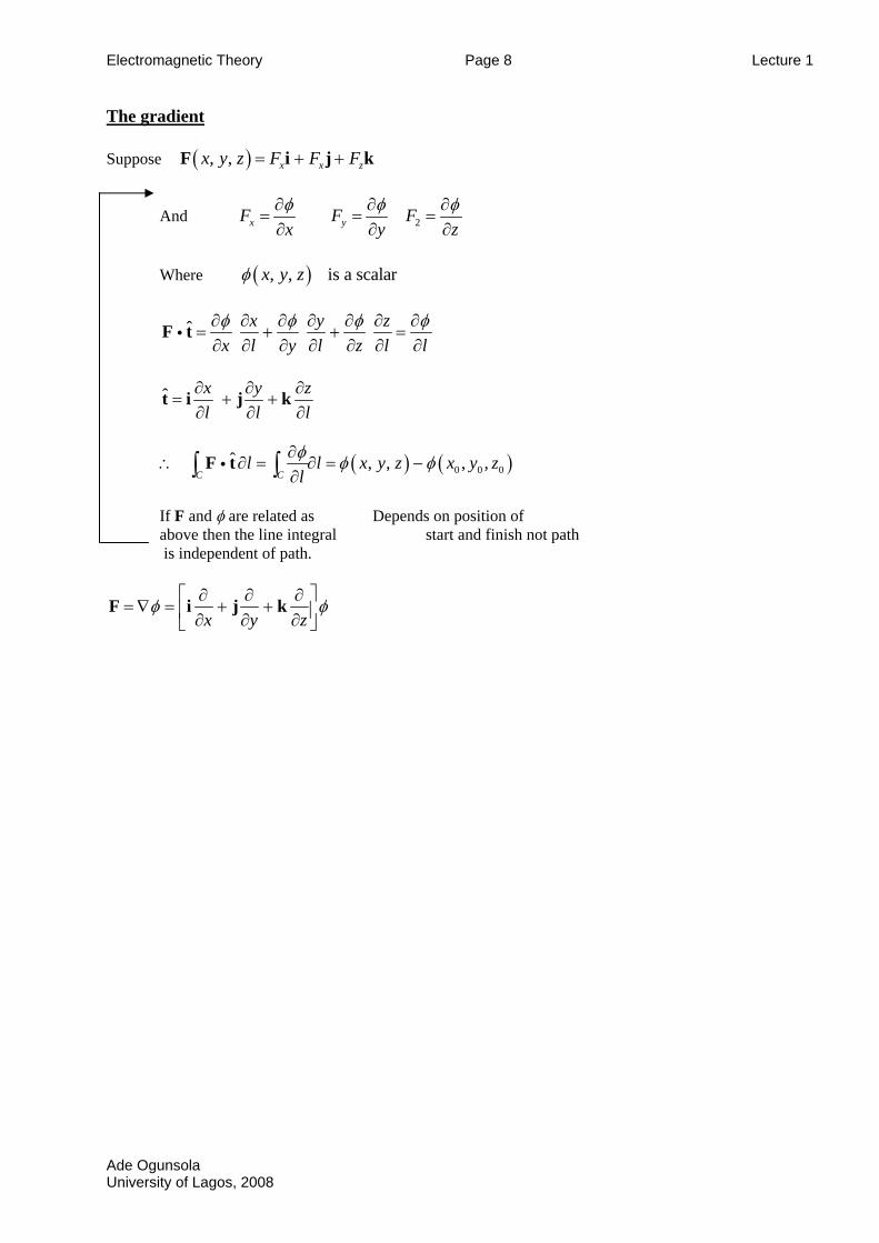
g of curl
r draining from a bathtub → not quite going to do this but → consider a small volume
y) where cossin
x r ty r t
ωω
==γ
) [, x y ]yt t
ω∂ ∂= + = − +
∂ ∂i j iy xi
ectrostatic field
ˆ ˆ0S
l s∂ = = ∇× ∂∫t n Ei i
0 for an electrostatic field∇× =E
velocity field 2ω∇× =V k
E cannot be an electrostatic field 0≠E
agos, 2008
Electromagnetic Theory Page 8 Lecture 1
The gradient Suppose ( ), , x x zx y z F F F= + +F i j k
And 2x yF F Fx y zφ φ φ∂ ∂ ∂
= = =∂ ∂ ∂
Where ( ), , is a scalarx y zφ
ˆ x y zx l y l z l lφ φ φ∂ ∂ ∂ ∂ ∂ ∂ ∂
= + + =∂ ∂ ∂ ∂ ∂ ∂ ∂
F ti φ
ˆ x y zl l
∂ ∂= + +
∂ ∂t i j k
l∂∂
( ) ( 0 0 0ˆ , , , ,
C Cl l x y z x y
l)zφ φ φ∂
∴ ∂ = ∂ = −∂∫ ∫F ti
If F and φ are related as Depends on position of above then the line integral start and finish not path is independent of path.
x y zφ φ
⎡ ⎤∂ ∂ ∂= ∇ = + +⎢ ⎥∂ ∂ ∂⎣ ⎦
F i j k
Ade Ogunsola University of Lagos, 2008
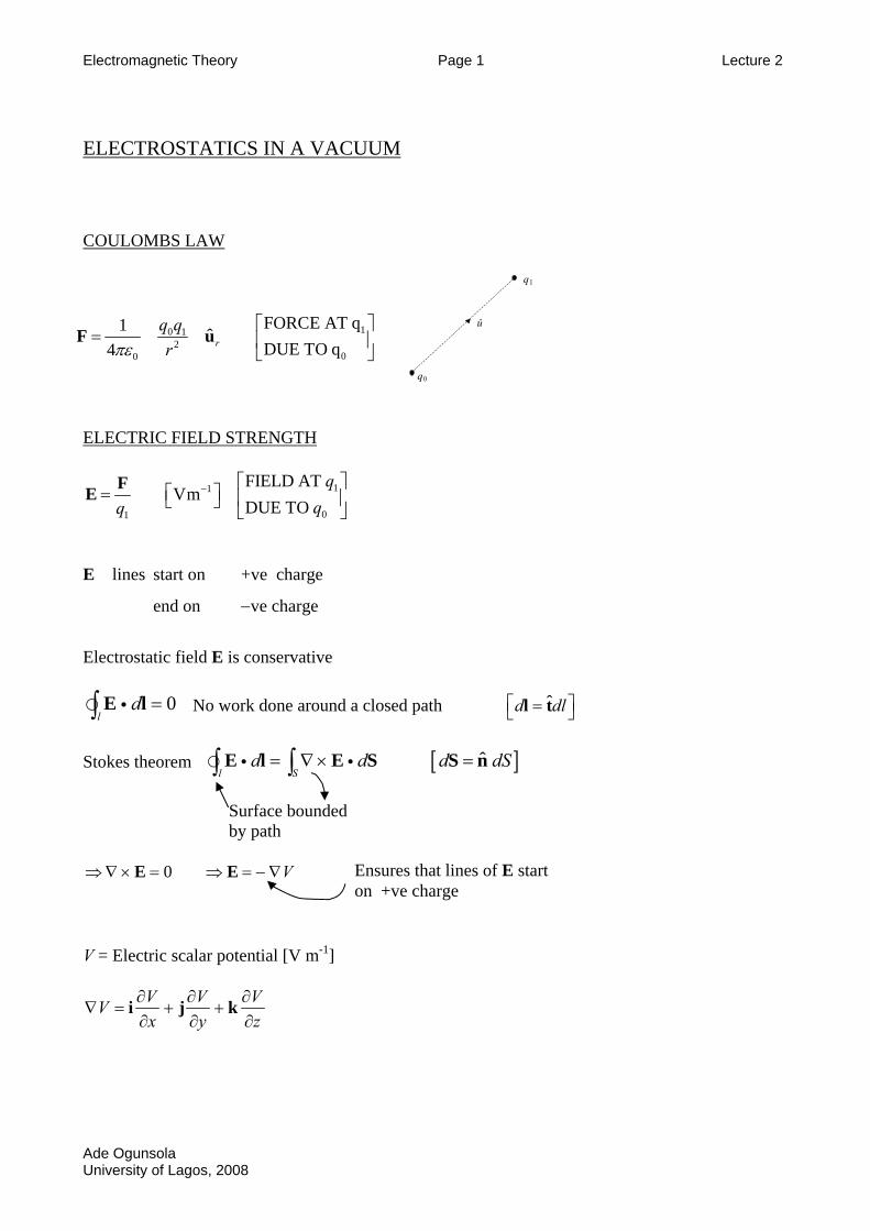
Electromagnetic Theory Page 1 Lecture 2 ELECTROSTATICS IN A VACUUM COULOMBS LAW
û
q1
FORCE AT q1 q q ⎡ ⎤
Ade Ogunsola
q0
10 12
00
ˆDUE TO q4 rrπε
= ⎢ ⎥⎣ ⎦
F u
ELECTRIC FIELD STRENGTH
11
01
FIELD ATVm
DUE TOq
qq− ⎡ ⎤
⎡ ⎤= ⎢ ⎥⎣ ⎦⎣ ⎦
FE
E lines start on +ve charge
end on −ve charge
Electrostatic field E is conservative
0l
d =∫ E li No work done around a closed path ˆd dl⎡ ⎤=⎣ ⎦l t
Stokes theorem [ ]ˆ
l Sd d d= ∇× =∫ ∫E l E S S ni i dS
⇒∇× = ⇒ =E E
Surface bounded by path
0 V− ∇ Ensures that lines of E start on +ve charge
V = Electric scalar potential [V m-1]
V VV Vx y z
∂ ∂ ∂∇ = + +
∂ ∂ ∂i j k
University of Lagos, 2008
Electromagnetic Theory Page 2 Lecture 2
Ade Ogunsola
ABSOLUTE POTENTIAL
A
AV∞
= − ∫ E i dl External work done per unit (+ve) charge to move unit test charge from
infinity to the point A. POTENTIAL DIFFERENCE
B
BA B A AV V V d= − = − ∫ E i l Work done per unit chare in moving unit test charge from A →B.
CHARGE DISTRIBUTION
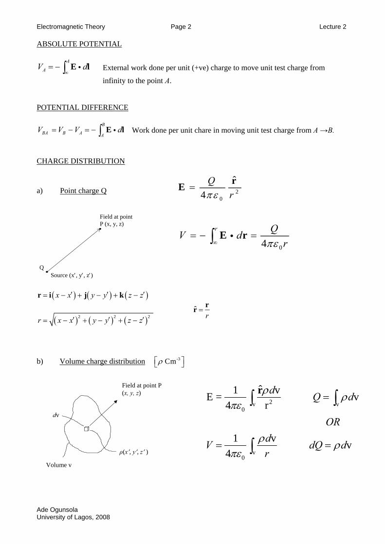
a) Point charge Q 20
ˆ4
Qrπε
=rE
Source (x′, y′, z′)
Field at point P (x, y, z)
Q
( ) ( ) ( )x x y y z′ ′= − + − + −r i j k z′
( ) ( ) ( )2 2 2r x x y y z z′ ′ ′= − + − + −
b) Volume charge distribution Cmρ⎡⎣
Field at point P (x, y, z)
ρ(x′, y′, z′ )
Volume v
dv
University of Lagos, 2008
r Q
04V d
rπε∞= − =∫ E ri
ˆr
=rr
-3 ⎤⎦
2v v
0
v0
ˆ1 v v4 r
1 v v4
d Q d
ORdV dQ dr
E = ρ ρπε
ρ ρπε
=
= =
∫ ∫
∫
r
Electromagnetic Theory Page 3 Lecture 2
Ade Ogunsola
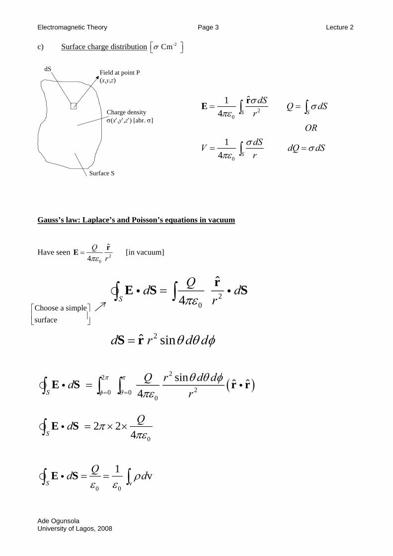
c) Surface charge distribution -2Cmσ⎡ ⎤⎣ ⎦ dS Field at point P
(x,y,z)
Charge density σ(x′,y′,z′) [abr. σ]
Surface S
ˆ1 dSσr
Gauss’s law: Laplace’s and Poisson’s equations
Have seen 20
ˆ4
Qrπε
=rE [in vacuum]
4S
Qdπε
=∫ ∫E Si
2ˆ sind r dθ θ=S r
22
20 00
sin4S
Q rdr
π π
φ θ
θπε= =
=∫ ∫ ∫E Si
0
2 24S
Qd ππε
= × ×∫ E Si
v0 0
1 vS
Qd dρε ε
= =∫ ∫E Si
Choose a simplesurface⎡ ⎤⎢ ⎥⎣ ⎦
University of Lagos, 2008
20
0
4
14
S S
S
Q dr
ORdSV dr
S
Q dS
σπε
σ σπε
= =
= =
∫ ∫
∫
E
in vacuum
20
ˆd
rr Si
dφ
( )ˆ ˆd dθ φ r ri
Electromagnetic Theory Page 4 Lecture 2
Ade Ogunsola
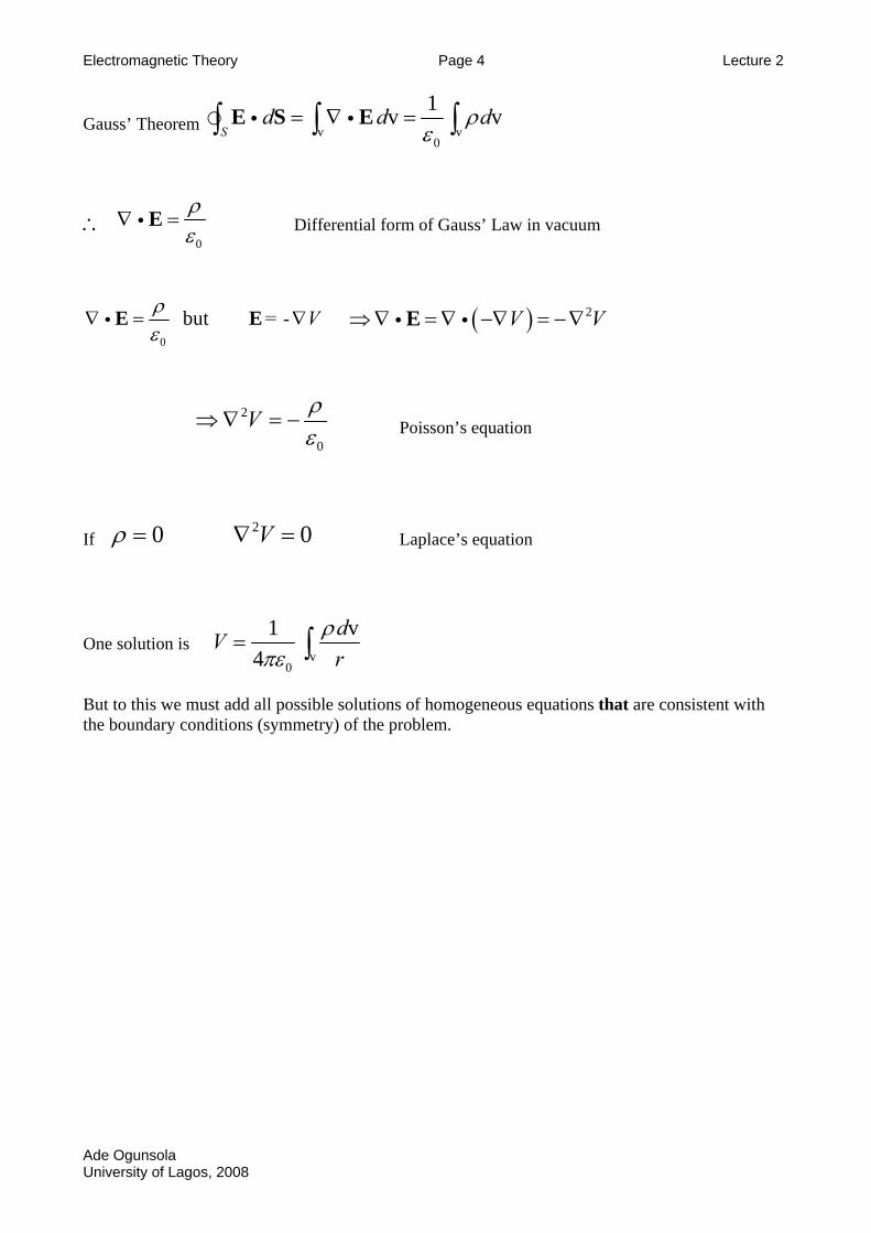
Gauss’ Theorem v v0
1v vS
d d dρε
= ∇ =∫ ∫ ∫E S Ei i
∴ 0
ρε
∇ =Ei Differential form of Gauss’ Law in vacuum
0
but = - Vρε
∇ = ∇E Ei ( ) 2V V⇒∇ =∇ −∇ = −∇Ei i
2
0
V ρε
⇒ ∇ Poisson’s equation = −
0=
If Laplace’s equation 20 Vρ = ∇
v0
1 v4
dVr
ρπε
= ∫One solution is But to this we must add all possible solutions of homogeneous equations that are consistent with the boundary conditions (symmetry) of the problem.
University of Lagos, 2008
Electromagnetic Theory Page 1 Lecture 2b
Ade Ogunsola
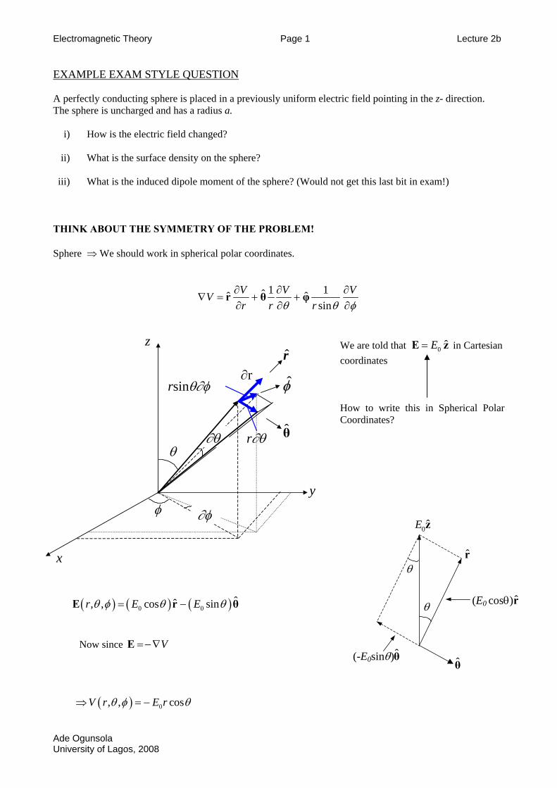
EXAMPLE EXAM STYLE QUESTION A perfectly conducting sphere is placed in a previously uniform electric field pointing in the z- direction. The sphere is uncharged and has a radius a.
i) How is the electric field changed?
ii) What is the surface density on the sphere? iii) What is the induced dipole moment of the sphere? (Would not get this last bit in exam!)
THINK ABOUT THE SYMMETRY OF THE PROBLEM! Sphere ⇒ We should work in spherical polar coordinates.
1 1ˆˆ ˆsin
V VVr r r
Vθ θ φ
∂ ∂ ∂∇ = + +
∂ ∂ ∂r θ φ
θ
φ
x
∂rr
rsinθ∂φ
r∂θ θ
φ
y
z
∂θ
∂φ
We are told that E in Cartesian coordinates
0 ˆE= z
How to write this in Spherical Polar Coordinates?
θθ
(-E0sinθ)
(E0 cosθ)r
θ
θ
r
0ˆE z
( ) ( ) ( )0 0ˆˆ, , cos sinr E Eθ φ θ= −E r θθ
Now since E V=−∇
( ) 0, , cosV r E rθ φ θ⇒ = −
University of Lagos, 2008
Electromagnetic Theory Page 2 Lecture 2b
Ade Ogunsola
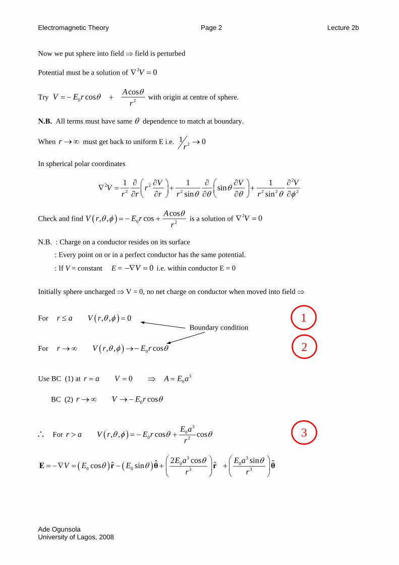
Now we put sphere into field ⇒ field is perturbed Potential must be a solution of 2 0V∇ =
Try 0 2
coscos AV E rr
θθ= − + with origin at centre of sphere.
N.B. All terms must have same θ dependence to match at boundary. When must get back to uniform E i.e. r →∞ 2
1 0r →
In spherical polar coordinates
22 2
2 2 2 2
1 1 1sinsin sin
V VV rr r r r r
θ 2
Vθ θ θ θ
∂ ∂ ∂ ∂ ∂⎛ ⎞ ⎛ ⎞∇ = + +⎜ ⎟ ⎜ ⎟∂ ∂ ∂ ∂ ∂⎝ ⎠ ⎝ ⎠ φ
Check and find ( ) 0 2
cos, , cos AV r E rr
θθ φ = − + is a solution of 2 0V∇ =
V r θ φ≤
r E r
N.B. : Charge on a conductor resides on its surface
: Every point on or in a perfect conductor has the same potential.
: If V = constant E = i.e. within conductor E = 0 0V−∇ =
Initially sphere uncharged ⇒ V = 0, no net charge on conductor when moved into field ⇒ For r a ( ), , 0= For r V ( ) 0, , cosθ φ θ→ ∞ →−
1
2
Boundary condition
Use BC (1) at 3
00r a V A E a= = ⇒ = BC (2) 0 cosr V E r θ→∞ →−
∴ For ( )3
00 2, , cos cosE ar a V r E r
rθ φ θ> = − + θ 3
( ) ( )3 3
0 00 0 3 3
2 cos sinˆ ˆˆ ˆcos sin E a E aV E Er r
θ θθ θ⎛ ⎞ ⎛
= −∇ = − + +⎜ ⎟ ⎜⎝ ⎠ ⎝
E r θ r θ⎞⎟⎠
University of Lagos, 2008
Electromagnetic Theory Page 3 Lecture 2b
Ade Ogunsola
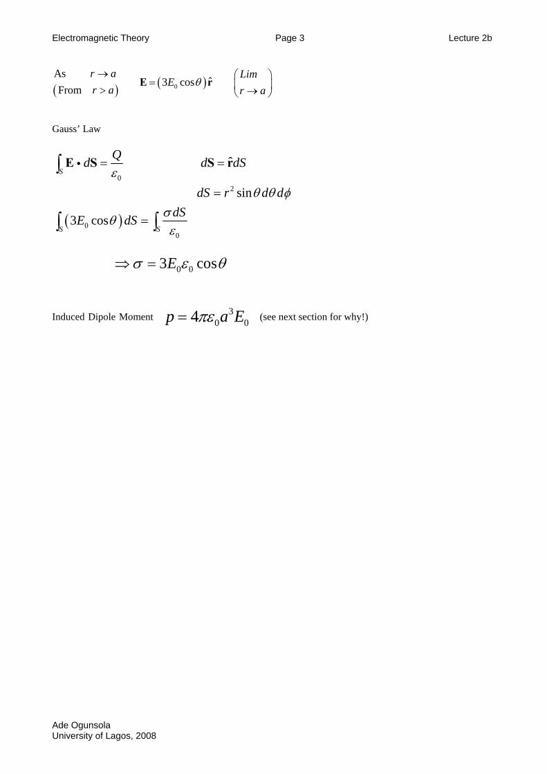
( ) ( )0
Asˆ3 cos
Fromr a Lim
Er a r a
θ→ ⎛ ⎞
= ⎜ ⎟> →⎝ ⎠E r
Gauss’ Law
( )
02
00
ˆ
sin
3 cos
S
S S
Qd d dS
dS r d ddSE dS
εθ θ φ
σθε
= =
=
=
∫
∫ ∫
E S S ri
0 03 cosEσ ε θ⇒ = Induced Dipole Moment (see next section for why!) 3
0 04p aπε= E
University of Lagos, 2008
Electromagnetic Theo Page 4 Lecture 2b
MAde
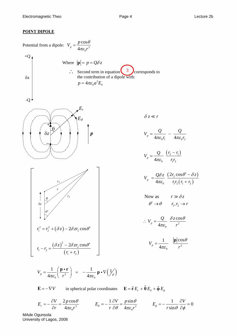
POINT DIPOLE
Potential from a dipole: 20
cos4ppV
rθ
πε=
+Q
-Q
δz
Where p Q zδ= =p
∴ Second term in equation corresponds to the contribution of a dipole with:
30 04p a Eπε=
3
Er
Eθ
θ δz
+
−
p
( )
( )( )
0 1
0 1
0 1
0
4
4
Now as
4
p
p
p
p
z r
V
QVr r
Q zV
Q zV
0 2
2 1
2
2
2 1 2
1 2
2
4 4
2 cos
,
cos
Q Qr r
r r
r zr r r r
r zr r r
r
δ
πε
πε
πε
θ δ
δ
δ θ
−
′ −+
→ →
δπε
θ θ
πε
= −
=
=
′
∴ =
θ
r
r1
r2
θ′
δz
( )2 2 2 cosr r z zrδ δ θ ′= + −
Univer
Ogunsola0
14pV 2
cosr
θπε
=p
( )( )
1 2 2
22
1 21 2
2 cosz zrr r
r rδ δ θ ′−
− =+
( )30 0
1 1 14 4pV rrπε πε
⎛ ⎞= = −⎜ ⎟⎝ ⎠
p r pi i∇
V= −∇E in spherical polar coordinates 0
ˆˆ ˆrE E Eφ= + +E r θ φ
30
2 cos4r
V pEr r
θπε
∂= − =
∂ 3
0
1 si4
V pEr rθ
nθθ πε∂
= − =∂
1 0
sinVE
rφ θ φ∂
= − =∂
sity of Lagos, 2008
Electromagnetic Theory Page 1 Lecture 3
THE ELECTROSTATIC PROPERTIES OF DIELECTRIC MATERIALS
IDEAL DIELECTRIC – contains no free charge (perfect insulator)
In practice all material media contain some free charges and therefore have
finite conductivity.
DIELECTRIC ⇒ very low electrical conductivity
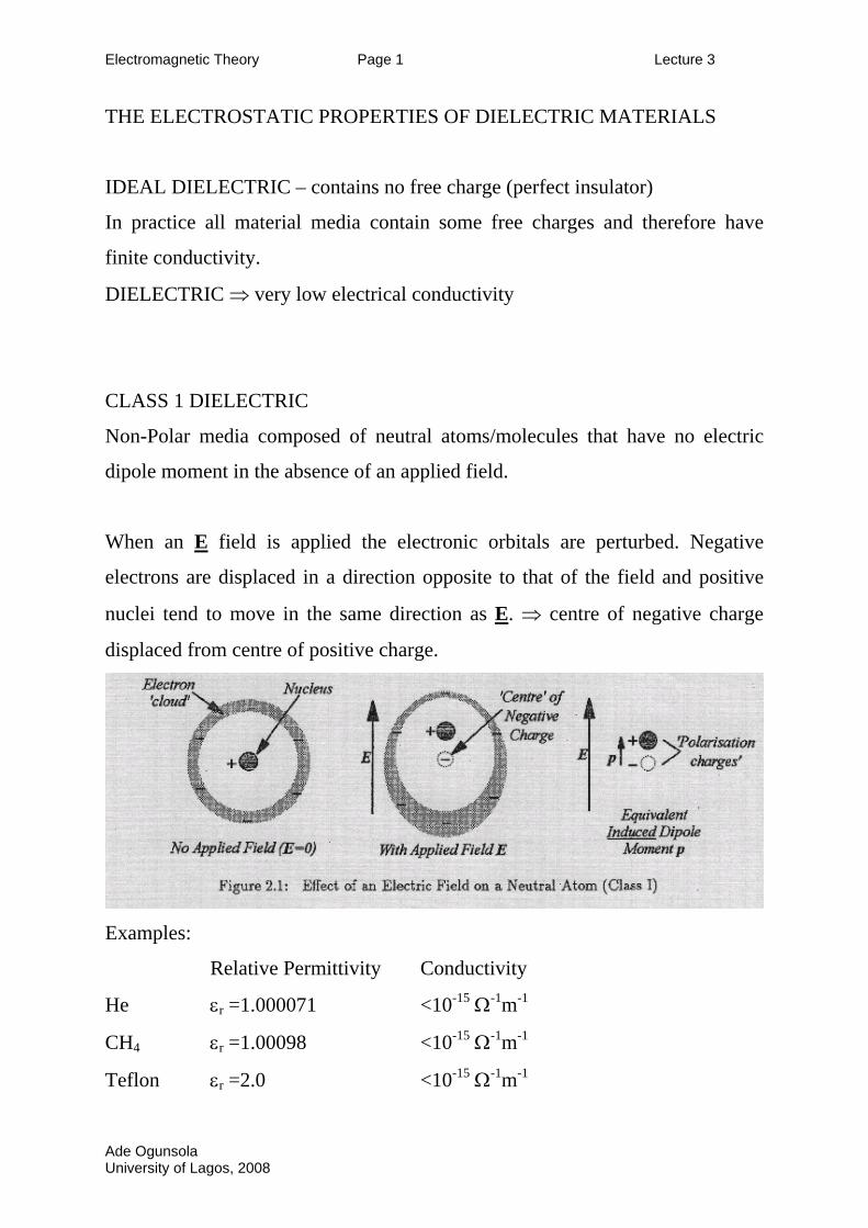
CLASS 1 DIELECTRIC
Non-Polar media composed of neutral atoms/molecules that have no electric
dipole moment in the absence of an applied field.
When an E field is applied the electronic orbitals are perturbed. Negative
electrons are displaced in a direction opposite to that of the field and positive
nuclei tend to move in the same direction as E. ⇒ centre of negative charge
displaced from centre of positive charge.
Examples:
Relative Permittivity Conductivity
He εr =1.000071 <10-15 Ω-1m-1
CH4 εr =1.00098 <10-15 Ω-1m-1
Teflon εr =2.0 <10-15 Ω-1m-1
Ade Ogunsola University of Lagos, 2008
Electromagnetic Theory Page 2 Lecture 3
CLASS II DIELECTRIC
Polar dielectric composed of molecules or ion pair that have a permanent
electric dipole moment.
Examples: H2O εr ≈ 80 @ low frequency and T>273K
KCl εr ≈ 5.0 @ low frequency and T=273K
NH3 εr ≈ 1.008 @ T=273K and 105 Pa
Consider a gas of polar molecules with each molecule having a Dipole Moment
pm. In the absence of an electric field the directions of these dipoles are
randomised by thermal energy. When E applied dipoles tend to align parallel to
E. The Tendency to align is disturbed by thermal motion. Since kBT >> pm.E
(pm.E – electrostatic energy of a dipole). The net moment of a volume of gas is
much smaller than it would be if all dipoles were aligned.
When E applied to a Polar Gas also get induced (type 1) dipole moments.
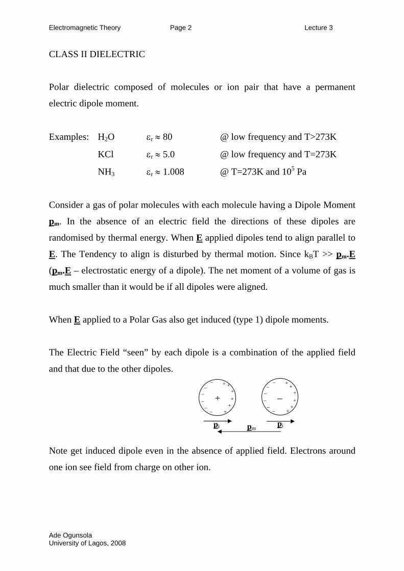
The Electric Field “seen” by each dipole is a combination of the applied field
and that due to the other dipoles. −
−
− −
− −
+ +
+
+ +
+ −
−
−
− −
− −
+ +
+
+ + +
+
pm pi pi
Note get induced dipole even in the absence of applied field. Electrons around
one ion see field from charge on other ion.
Ade Ogunsola University of Lagos, 2008
Electromagnetic Theory Page 3 Lecture 3
SOLIDS AND LIQUIDS
TYPE 1 DIELECTRIC – Simple approach works OK
TYPE 2 DIELECTRIC – Complicated
E.G. H2O εr ≈ 80 for water at T ≥ 273K
H2O εr ≈ 3 for ice
In ice permanent dipoles cannot re-orientate!
In ionic solids small displacement of positive and negative ions caused by E
gives rise to large electric polarisation and εr – see solid-state physics…
DIELECTRIC BREAKDOWN
In E field the few free electric charges in a dielectric are accelerated – if the
field large enough then when these electrons collide with atoms (or ions) they
produce secondary electrons that are themselves accelerated by E.
⇒ AVALANCHE EFFECT – currents flows (in streamers) Dielectric is heated
and can be permanently damaged.
Field required for this effect – BREAKDOWN FIELD – typically 106 Vm-1
If dielectric thin (say in a commercial capacitor) a few volts can cause
breakdown.
Ade Ogunsola University of Lagos, 2008
Electromagnetic Theory Page 4 Lecture 3
DIELECTRIC POLARISATION (P) AND ELECTRIC SUSCEPTIBILITY (χ).
For both Class 1 and Class 2 Dielectrics, applied electric field INDUCES an
electric dipole moment in each elementary volume of the material. Induced
Dipole moment originates from POLARISATION CHARGES – bound to the
nuclei and not able to move as free charges.
Macroscopic measure of the induced-dipole effect is the ELECTRICAL
POLARISATION P.
P = Induced electric dipole moment / unit volume [ Cm-2]
Usually we write EP χε0=
Not always the whole truth! Assumes that P depends linearly on E.
χ homogeneous
P parallel to E.
P IS RELATED TO SURFACE AND BULK POLARISATION CHARGE
When a dielectric acquires an Electric Polarisation P (by virtue of an internal
field E ).
(a) A distribution of polarisation charges appears on the surface –surface
polarisation charge density nP ˆ•=pσ [Cm-2]. n is outwardly
directed unit vector normal to the surface.
Ade Ogunsola University of Lagos, 2008
Electromagnetic Theory Page 5 Lecture 3
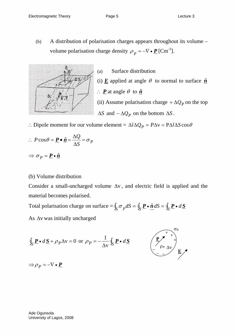
(b) A distribution of polarisation charges appears throughout its volume –
volume polarisation charge density P•−∇=pρ [Cm-3].
(a) Surface distribution
n(i) E applied at angle θ to normal to surface
∴P at angle θ to n ˆ
∆(ii) Assume polarisation charge + on the top PQ
S∆ and PQ∆− on the bottom S∆ .
∴Dipole moment for our volume element = θcosPv SlPQl P ∆∆=∆=∆∆
∴ PSQP σθ =∆∆
=•= nP ˆcos
⇒ nP ˆ•=Pσ
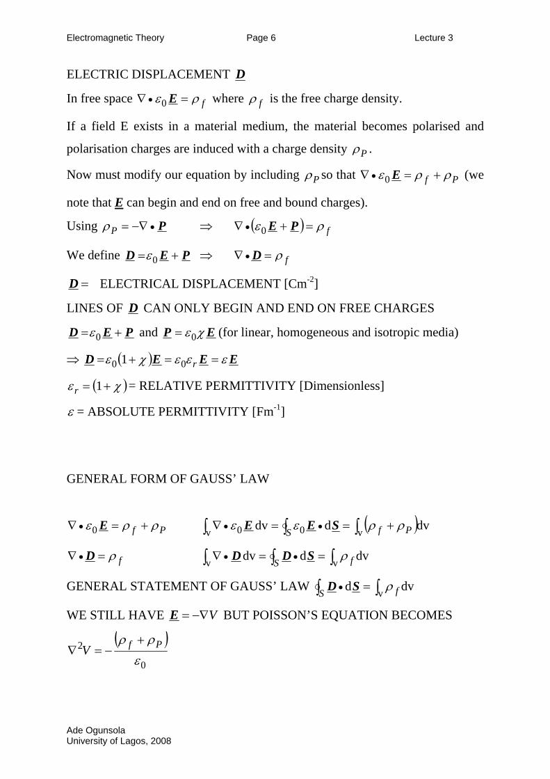
(b) Volume distribution
Consider a small-uncharged volume v∆ , and electric field is applied and the
material becomes polarised.
Total polarisation charge on surface = ∫∫∫ •• == SSS p ddSdS SPnP ˆσ
As ∆ was initially uncharged v
E ∆v
σP
−ρP
P
−−
+ +
+
0v =∆+∫ • PS d ρSP or ∫ •∆
−= SP d SPv
1ρ
⇒ P•−∇=Pρ
Ade Ogunsola University of Lagos, 2008
Electromagnetic Theory Page 6 Lecture 3
ELECTRIC DISPLACEMENT D
In free space fρε =∇ • E0 where fρ is the free charge density.
If a field E exists in a material medium, the material becomes polarised and
polarisation charges are induced with a charge density Pρ .
Now must modify our equation by including Pρ so that Pf ρρε +=∇ • E0 (we
note that E can begin and end on free and bound charges).
Using P•−∇=Pρ ⇒ ( ) fρε =+∇ • PE0
We define PED += 0ε ⇒ fρ=∇ •D
=D ELECTRICAL DISPLACEMENT [Cm-2]
LINES OF D CAN ONLY BEGIN AND END ON FREE CHARGES
PED += 0ε and EP χε0= (for linear, homogeneous and isotropic media)
⇒ ( ) EEED εεεχε ==+= r00 1
( )χε += 1r = RELATIVE PERMITTIVITY [Dimensionless]
ε = ABSOLUTE PERMITTIVITY [Fm-1]
GENERAL FORM OF GAUSS’ LAW
Pf ρρε +=∇ • E0 ( )∫∫∫ +==∇ •• v0v 0 dvddv PfS ρρεε SEE
fρ=∇ •D ∫∫∫ ==∇ •• vv dvddv fS ρSDD
GENERAL STATEMENT OF GAUSS’ LAW ∫∫ =• v dvd fS ρSD
WE STILL HAVE V−∇=E BUT POISSON’S EQUATION BECOMES
( )0
2ερρ PfV
+−=∇
Ade Ogunsola University of Lagos, 2008
Electromagnetic Theory Page 7 Lecture 3
FIELDS NEAR A CHARGED CONDUCTOR
Lines of D and E are normal to the surface close to the surface (we have seen
this before and will see it again with boundary conditions).
Gauss’s Law fS Sd σ• =∫ ∫D S dS since all free charge on surface.
Just above surface SSD fn ∆=∆ σ and fnD σ= and 0ε
σ fnE =
0=nE in conductor since potential everywhere in conductor is the same –
uniform potential.
EXAMPLES CONCERNING POLARISATION CHARGES
(a) Relation between Pρ and fρ for a simple linear, homogeneous medium ⇒
=rε constant
PED += 0ε and ED rεε0=
∴ ⎟⎟⎠
⎞⎜⎜⎝
⎛ −=−=
r
r
r εε
εεε 1
0
0 DDDP
⇒ DP •• ∇⎟⎟⎠
⎞⎜⎜⎝
⎛ −=∇
r
rε
ε 1 and since fρ=∇ •D and P•−∇=Pρ then
fr
rP ρ
εε
ρ ⎟⎟⎠
⎞⎜⎜⎝
⎛ −−=
1. So if 0=fρ then 0=Pρ ⇒ only a surface charge
distribution Pσ exists on polarised medium.
Ade Ogunsola UNiversity of Lagos, 2008
Electromagnetic Theory Page 8 Lecture 3
EFFECTIVE CHARGE DENSITY
Pf ρρε +=∇ • E0 so in linear homogeneous medium fr
rP ρ
εε
ρ ⎟⎟⎠
⎞⎜⎜⎝
⎛ −−=
1 then
r
f
ερ
ε =∇ • E0 . r
f
ερ
is called the effective charge density.
∴If a point charge Q is placed in an dielectric medium the effective charge is
r
Qε
which is less than Q since .1>rε Physical Reason: On the surface of the
dielectric adjacent to the point charge Q there is a surface distribution of
polarisation charge of the opposite sign to Q – reducing the effective charge
(see the problem sheet).
Ade Ogunsola University of Lagos, 2008
Electromagnetic Theory Page 1 Lecture 4
BOUNDARY CONDITIONS IN ELECTROSTATICS THE NORMAL COMPONENT OF D IS CONTINUOUS ACROSS
A BOUNDARY PROVIDED THAT NO FREE CHARGE IS PRESENT ON THE BOUNDARY.
THE TANGENTIAL COMPONENT OF E IS CONTINUOUS
ACROSS A BOUNDARY.
ANY SOLUTION TO AN ELECTROSTATICS PROBLEM MUST SATISFY THE BOUNDARY CONDITIONS.
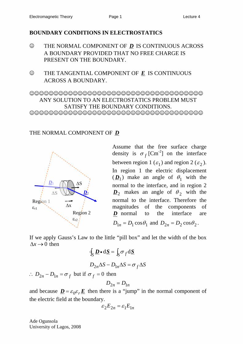
THE NORMAL COMPONENT OF D
Assume that the free surface charge density is fσ [Cm-2] on the interface between region 1 (
D1
Region 1 εr1
∆S D2
Region 2 εr2
∆x
∆S
) and region 2 (1ε 2ε ). In region 1 the electric displacement ( 1D ) make an angle of 1θ with the normal to the interface, and in region 2
2D makes an angle of 2θ with the normal to the interface. Therefore the magnitudes of the components of D normal to the interface are
111 cosθDD n = and 222 cosθDD n = .
If we apply Gauss’s Law to the little “pill box” and let the width of the box 0→∆x then
SSDSD fnn
fS
∆=∆−∆
= ∫∫ •
σ
σ
12
S dd SSD
∴ fnn DD σ=− 12 but if 0=fσ then
nn DD 12 = and because ED rεε0= then there is a “jump” in the normal component of the electric field at the boundary.
nn EE 1122 εε =
Ade Ogunsola University of Lagos, 2008
Electromagnetic Theory Page 2 Lecture 4
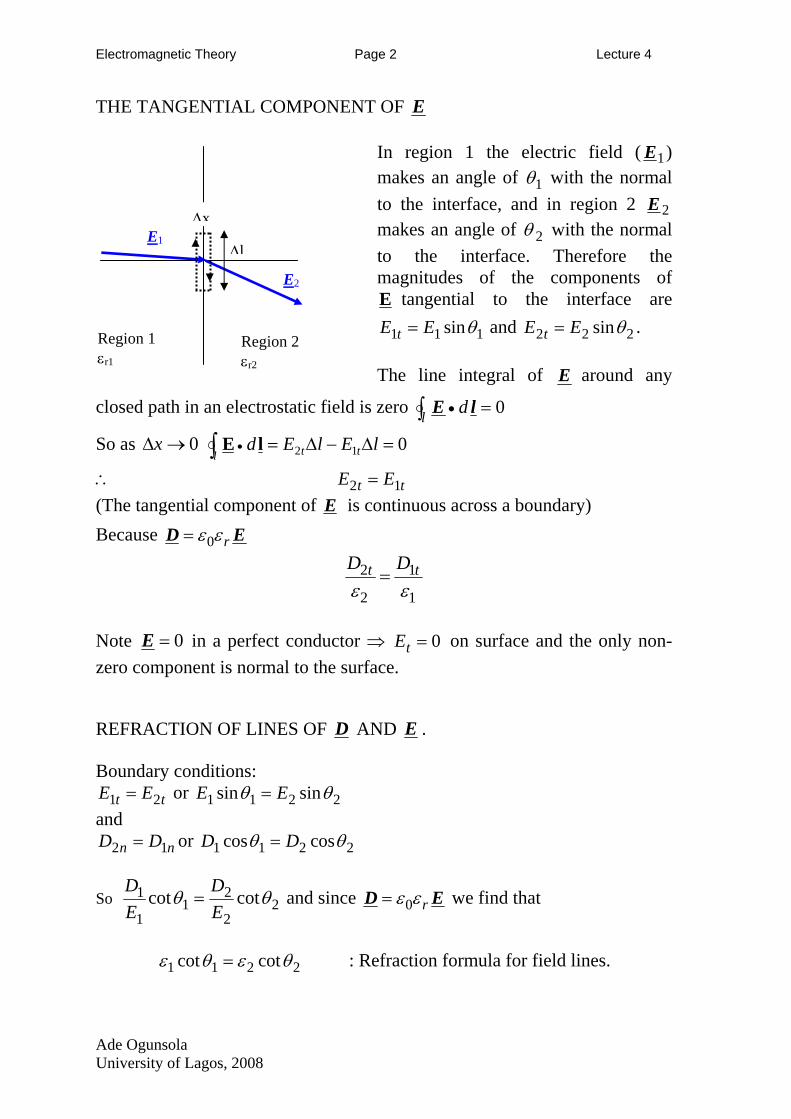
THE TANGENTIAL COMPONENT OF E
1EIn region 1 the electric field ( ) makes an angle of 1θ with the normal to the interface, and in region 2 2E makes an angle of 2θ with the normal to the interface. Therefore the magnitudes of the components of E tangential to the interface are
111 sinθEE t = and 222 sinθEE t = . The line integral of E around any
closed path in an electrostatic field is zero 0=∫ •l d lE
E2
E1
Region 1 εr1
∆l
∆x
Region 2 εr2
So as 0→∆x 012 =∆−∆=∫ • lElEd ttllE
∴ tt EE 12 = (The tangential component of E is continuous across a boundary) Because ED rεε0=
1
1
2
2εε
tt DD=
Note 0=E in a perfect conductor ⇒ 0=tE on surface and the only non-zero component is normal to the surface. REFRACTION OF LINES OF D AND E . Boundary conditions:
tt EE 21 = or 2211 sinsin θθ EE = and
nn DD 12 = or 2211 coscos θθ DD =
So 22
21
1
1 cotcot θθED
ED
= and since ED rεε0= we find that
2211 cotcot θεθε = : Refraction formula for field lines.
Ade Ogunsola University of Lagos, 2008
Electromagnetic Theory Page 3 Lecture 4
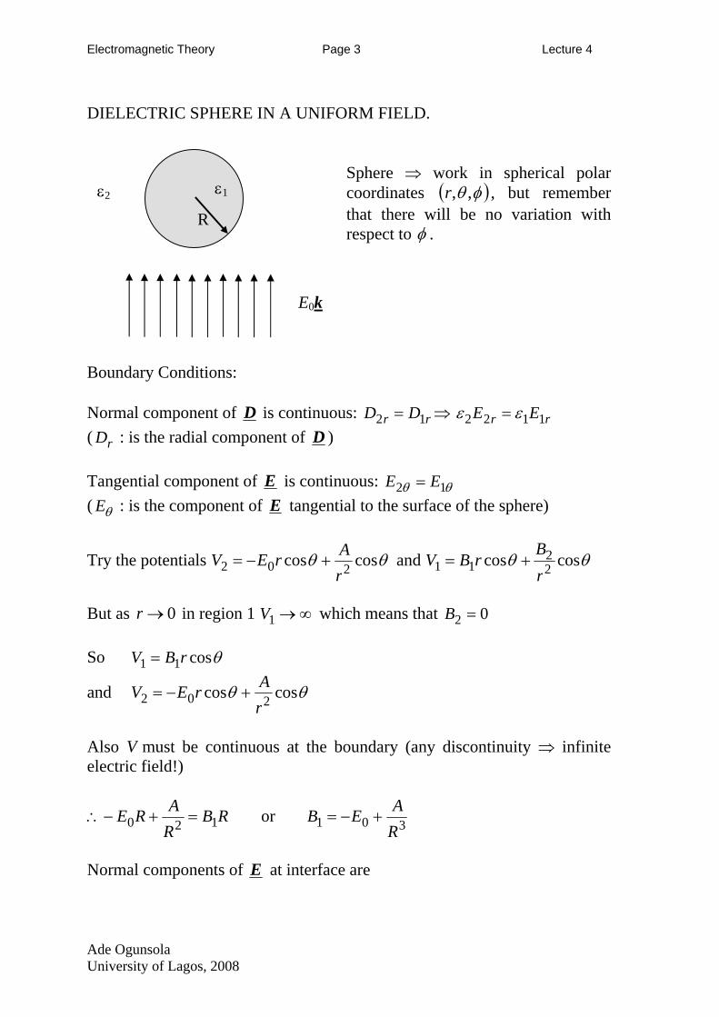
DIELECTRIC SPHERE IN A UNIFORM FIELD.
ε1
R
Sphere ⇒ work in spherical polar coordinates ( )φθ ,,r , but remember that there will be no variation with respect to φ .
ε2
E0k
Boundary Conditions: Normal component of D is continuous: rr DD 12 = ⇒ rr EE 1122 εε = ( : is the radial component of rD D ) Tangential component of E is continuous: θθ 12 EE = ( : is the component of θE E tangential to the surface of the sphere)
Try the potentials θθ coscos 202 rArEV +−= and θθ coscos 2
211 r
BrBV +=
But as 0→r in region 1 ∞→1V which means that 02 =B So θcos11 rBV =
and θθ coscos 202 rArEV +−=
Also V must be continuous at the boundary (any discontinuity ⇒ infinite electric field!)
∴ RBRARE 120 =+− or 301 R
AEB +−=
Normal components of E at interface are
Ade Ogunsola University of Lagos, 2008
Electromagnetic Theory Page 4 Lecture 4
θcos11
1 Br
VE
Rrr −=⎥
⎦
⎤⎢⎣
⎡∂∂
−==
θθ cos2cos 302
2 RAE
rV
ERr
r +=⎥⎦
⎤⎢⎣
⎡∂∂
−==
We know rr EE 1122 εε = so
32
02112R
AEB
εεε +=− or ⎥⎦
⎤⎢⎣⎡ +−= 30
1
21
2R
AEBεε
So 30301
2 2RAE
RAE +−=⎥⎦⎤
⎢⎣⎡ +−
εε
so ( )( ) 0
3
21
212
ERAεεεε
+−
= and ( ) 021
21 2
3EB
εεε
+−
=
( ) θεεε
cos2
30
21
21 rEV
+−
= and ( )( ) θ
εεεε
cos2
1 03
3
21
212 rE
rRV ⎟
⎟⎠
⎞⎜⎜⎝
⎛
+−
−−=
Hence at Rr =
( )( )( ) kEkEkE ˆ
2ˆˆ
23
021
1200
21
21 εε
εεεε
ε+−
+=+
=E
Consider Dielectric sphere in vacuum 02 εε = and rεεε 01 =
∴( )( ) kEkE
r
r ˆ2
1ˆ001 +
−+=ε
εE
but ( ) kEP r
ˆ1 101 −= εε
( )( ) kEP
r
r ˆ2
130
01 +
−=
εεε
∴ 0
101 3
ˆεPkE −=E
Ade Ogunsola University of Lagos, 2008
Electromagnetic Theory Page 5 Lecture 4
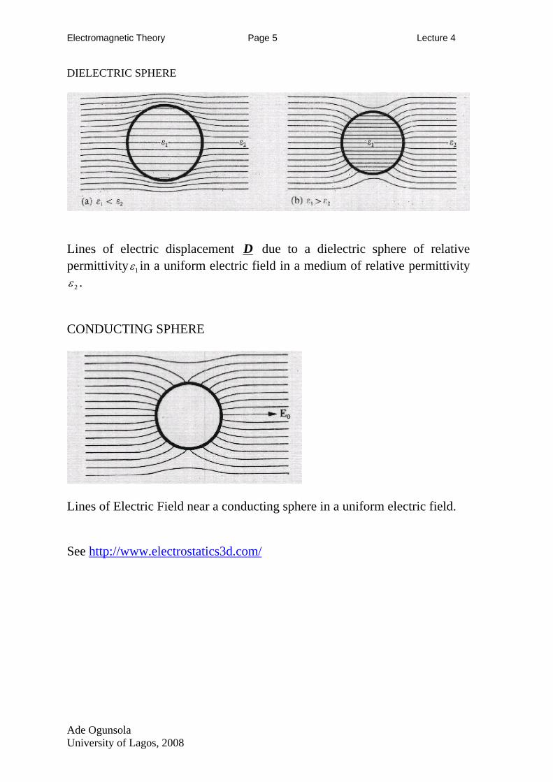
DIELECTRIC SPHERE
Lines of electric displacement D due to a dielectric sphere of relative permittivity 1ε in a uniform electric field in a medium of relative permittivity
2ε . CONDUCTING SPHERE
Lines of Electric Field near a conducting sphere in a uniform electric field. See http://www.electrostatics3d.com/
Ade Ogunsola University of Lagos, 2008
Electromagnetic Theory Page 1 Lecture 5
CAPACITANCE To calculate the capacitance of any given arrangement we must calculate the P.D. between the conductors for an assumed charge. METHOD
1. Assume charge on either conductor Q± 2. Use GAUSS’ LAW to find D in the space between the conductors.
3. Calculate E at each point in space using ED rεε0= . 4. Find the P.D. between the conductors from ∫ •−= l dV lE along any
path joining the conductors.
5. VQC = .
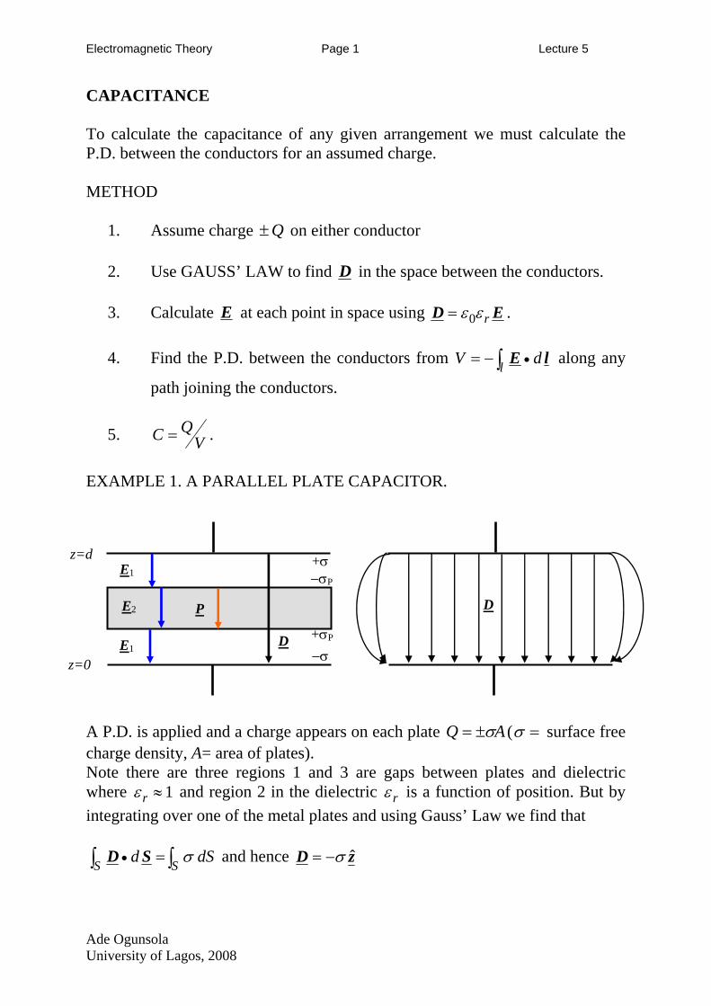
EXAMPLE 1. A PARALLEL PLATE CAPACITOR.
D
+σ−σP
+σP
−σ
DPE2
E1
E1
z=d
z=0
A P.D. is applied and a charge appears on each plate AQ σ±= ( =σ surface free charge density, A= area of plates). Note there are three regions 1 and 3 are gaps between plates and dielectric where 1≈rε and region 2 in the dielectric rε is a function of position. But by integrating over one of the metal plates and using Gauss’ Law we find that
∫∫ =• SS dSd σSD and hence zD ˆσ−=
Ade Ogunsola University of Lagos, 2008
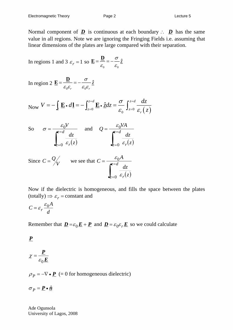
Electromagnetic Theory Page 2 Lecture 5
Normal component of D is continuous at each boundary ∴ D has the same value in all regions. Note we are ignoring the Fringing Fields i.e. assuming that linear dimensions of the plates are large compared with their separation.
In regions 1 and 3 1=rε so 0 0
zσε ε
= = −DE
In region 2 0 0
ˆr r
zσε ε ε ε
= = −DE
Now ( )0 00
ˆz d z d
l z zr
dzV d zdzz
σε ε
= =• •
= == − = − =∫ ∫ ∫E l E
So
( )∫=
=
= dz
z r zdz
V
0
0
ε
εσ and
( )∫=
=
= dz
z r zdz
VAQ
0
0
ε
ε
Since VQC = we see that
( )∫=
=
= dz
z r zdz
AC
0
0
ε
ε
Now if the dielectric is homogeneous, and fills the space between the plates (totally) ⇒ =rε constant and
dA
C r0εε=
Remember that PED += 0ε and ED rεε0= so we could calculate P
EP
0εχ =
P•−∇=Pρ (= 0 for homogeneous dielectric)
nP ˆ•=Pσ
Ade Ogunsola University of Lagos, 2008
Electromagnetic Theory Page 3 Lecture 5
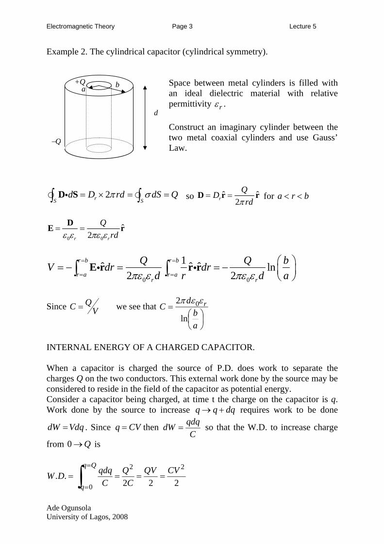
Example 2. The cylindrical capacitor (cylindrical symmetry).
b a +Q Space between metal cylinders is filled with
an ideal dielectric material with relative permittivity rε .
d Construct an imaginary cylinder between the two metal coaxial cylinders and use Gauss’ Law.
−Q
2rS Sd D rd dSπ σ= × = =∫ ∫D Si Q so ˆ ˆ
2rQDrdπ
= =D r for r bra <<
0 0
ˆ2r r
Qrdε ε πε ε
= =DE r
0 0
1ˆ ˆ ˆ ln2 2
r b r b
r a r ar r
Q QV dr drd r d aπε ε πε ε
= =
= =
⎛ ⎞= − = = − ⎜ ⎟⎝ ⎠∫ ∫E r r ri i b
Since VQC we see that =
⎟⎠⎞
⎜⎝⎛
=
ab
dC r
ln
2 0εεπ
INTERNAL ENERGY OF A CHARGED CAPACITOR. When a capacitor is charged the source of P.D. does work to separate the charges Q on the two conductors. This external work done by the source may be considered to reside in the field of the capacitor as potential energy. Consider a capacitor being charged, at time t the charge on the capacitor is q. Work done by the source to increase dqqq +→ requires work to be done
. Since VdqdW = CVq = then C
qdqdW = so that the W.D. to increase charge
from is Q→0
222..
22
0
CVQVC
QC
qdqDWQq
q==== ∫
=
=
Ade Ogunsola University of Lagos, 2008
Electromagnetic Theory Page 4 Lecture 5
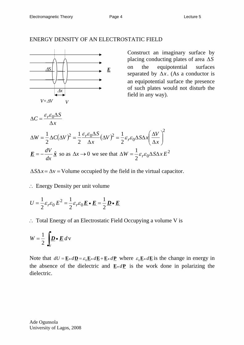
ENERGY DENSITY OF AN ELECTROSTATIC FIELD
Construct an imaginary surface by placing conducting plates of area S∆ on the equipotential surfaces separated by x∆ . (As a conductor is an equipotential surface the presence of such plates would not disturb the field in any way).
∆S
∆x
E
V+∆V V
xS
C r∆∆
=∆ 0εε
( ) ( )2
0202
21
21
21
⎟⎟⎠
⎞⎜⎜⎝
⎛∆∆
∆∆=∆∆∆
=∆∆=∆xVxSV
xS
VCW rr εεεε
xE ˆdxdV
−= so as 0→∆x we see that 202
1 ExSW r ∆∆=∆ εε
=∆=∆∆ vxS Volume occupied by the field in the virtual capacitor.
∴ Energy Density per unit volume
EDEE •• ===21
21
21
02
0 εεεε rr EU
∴ Total Energy of an Electrostatic Field Occupying a volume V is
v21
vdW ∫ •= ED
Note that 0dU d d dε• •= = +E D E E E P• where 0 dε •E E is the change in energy in the absence of the dielectric and d•E P is the work done in polarizing the dielectric.
Ade Ogunsola University of Lagos, 2008
Electromagnetic Theory Page 5 Lecture 5
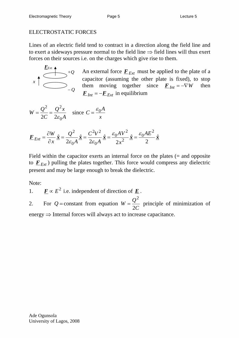
ELECTROSTATIC FORCES Lines of an electric field tend to contract in a direction along the field line and to exert a sideways pressure normal to the field line ⇒ field lines will thus exert forces on their sources i.e. on the charges which give rise to them.
FExt
− Q
+Q An external force ExtF must be applied to the plate of a capacitor (assuming the other plate is fixed), to stop them moving together since W−∇=IntF then
ExtInt FF −= in equilibrium
x
AxQ
CQW
0
22
22 ε== since
xA
C 0ε=
xxxxxF ˆ2
ˆ2
ˆ2
ˆ2
ˆ2
02
20
0
22
0
2 AExAV
AVC
AQ
xW
Extεε
εε====
∂∂
=
Field within the capacitor exerts an internal force on the plates (= and opposite to ExtF ) pulling the plates together. This force would compress any dielectric present and may be large enough to break the dielectric. Note: 1. 2E∝F i.e. independent of direction of E .
2. For =Q constant from equation C
QW principle of minimization of
energy ⇒ Internal forces will always act to increase capacitance. 2
2=
Ade Ogunsola University of Lagos, 2008
Electromagnetic Theory Page 6 Lecture 5
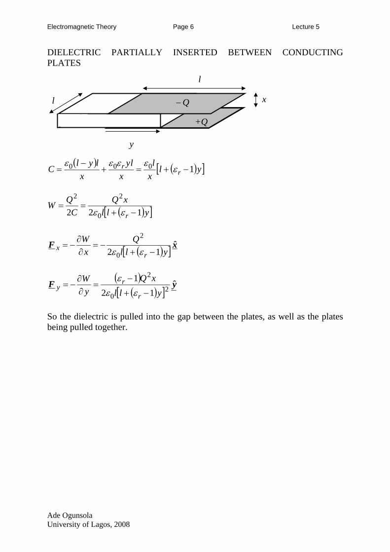
DIELECTRIC PARTIALLY INSERTED BETWEEN CONDUCTING PLATES
l
− Q
+Q
l x y
( ) ( )[ ]ylxl
xly
xlyl
C rr 1000 −+=+
−= ε
εεεε
( )[ ]yllxQ
CQW
r 122 0
22
−+==
εε
( )[ ] xF ˆ12 0
2
yllQ
xW
rx −+
−=∂∂
−=εε
( )
( )[ ]yF ˆ
121
20
2
yllxQ
yW
r
ry
−+
−=
∂∂
−=εε
ε
So the dielectric is pulled into the gap between the plates, as well as the plates being pulled together.
Ade Ogunsola University of Lagos, 2008
Electromagnetic Theory Page 1 Lecture 6
MAGNETIC EFFECTS OF CURRENTS AND MAGNETOSTATICS MAGNETIC EFFECTS OF CURRENTS Ampere, Oested, Biot, Savart….
• Two long parallel wires carrying currents in opposite directions repel one another where as when the currents are in the same direction they attract one another.
• If a wire carrying a current is placed near a magnet it experiences a force.
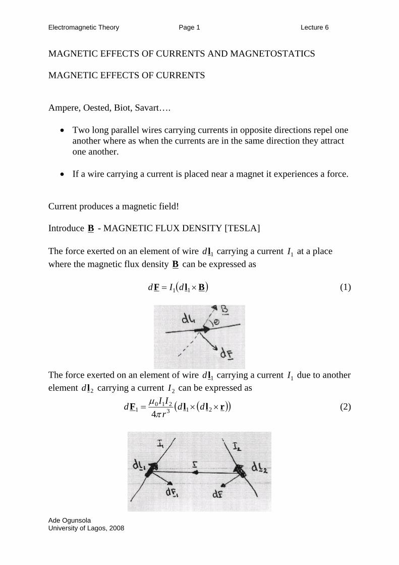
Current produces a magnetic field! Introduce B - MAGNETIC FLUX DENSITY [TESLA] The force exerted on an element of wire 1ld carrying a current at a place where the magnetic flux density
1IB can be expressed as
( )BlF ×= 11 dId (1)
The force exerted on an element of wire 1ld carrying a current due to another element
1I2ld carrying a current can be expressed as 2I
(( rllF ××= 213210
1 4dd
rIId
π))µ (2)
Ade Ogunsola University of Lagos, 2008
Electromagnetic Theory Page 2 Lecture 6
If we compare (1) and (2) we may say that the current in the element 2I 2ld produces a magnetic flux density Bd at a distance r where
( rlB ×= 2320
4d
rId
π)µ (3)
7
0 104 −×= πµ NA-2. Can use (3) to calculate B since
( )3
0
4 rdI
l
rlB ×= ∫πµ
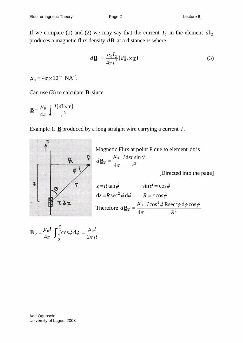
Example 1. B produced by a long straight wire carrying a current I .
Magnetic Flux at point P due to element zd is
30 sind
4 rrzId P
θπµ
=B
[Directed into the page]
φφφ
φθφ
cosdsecd
cossintan2 rRRz
Rz
==
==
Therefore 2
220 cosdRseccos
4 RId P
φφφφπµ
=B
RII
P πµφφ
πµ π
π 2dcos
402
2
0 == ∫+
−B
Ade Ogunsola University of Lagos, 2008
Electromagnetic Theory Page 3 Lecture 6
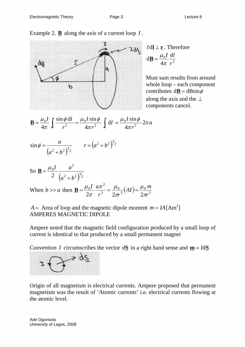
Example 2. B along the axis of a current loop I .
rl ⊥dI . Therefore
20 d
4d
rlI
πµ
=B
Must sum results from awhole loop – each componecontributes
round nt
φdBsind =B and the ⊥
components cancel.
along the axis
ar
Ilr
Ir
lIll
ππ
φµπ
φµφπ
µ 24
sind4
sindsin4 2
02
02
0 === ∫∫B
( )( ) 2
122
2122
sin barba
a+=
+=φ
( ) 2322
20
2 ba
aI
+=µB So
When then ab >> ( ) 30
30
3
20
222 rmAI
rraI
πµ
πµπ
πµ
===B
A = Area of loop and the magnetic dipole moment IAm = [Am2] AM
mpere noted that the magnetic field configuration produced by a small loop of
onvention
PERES MAGNETIC DIPOLE Acurrent is identical to that produced by a small permanent magnet
I circumscribes the vector Sd in a right hand sense and Sm dI= C
rigin of all magnetism is electrical currents. Ampere proposed that permanent Omagnetism was the result of ‘Atomic currents’ i.e. electrical currents flowing at the atomic level.
Ade Ogunsola University of Lagos, 2008
Electromagnetic Theory Page 4 Lecture 6
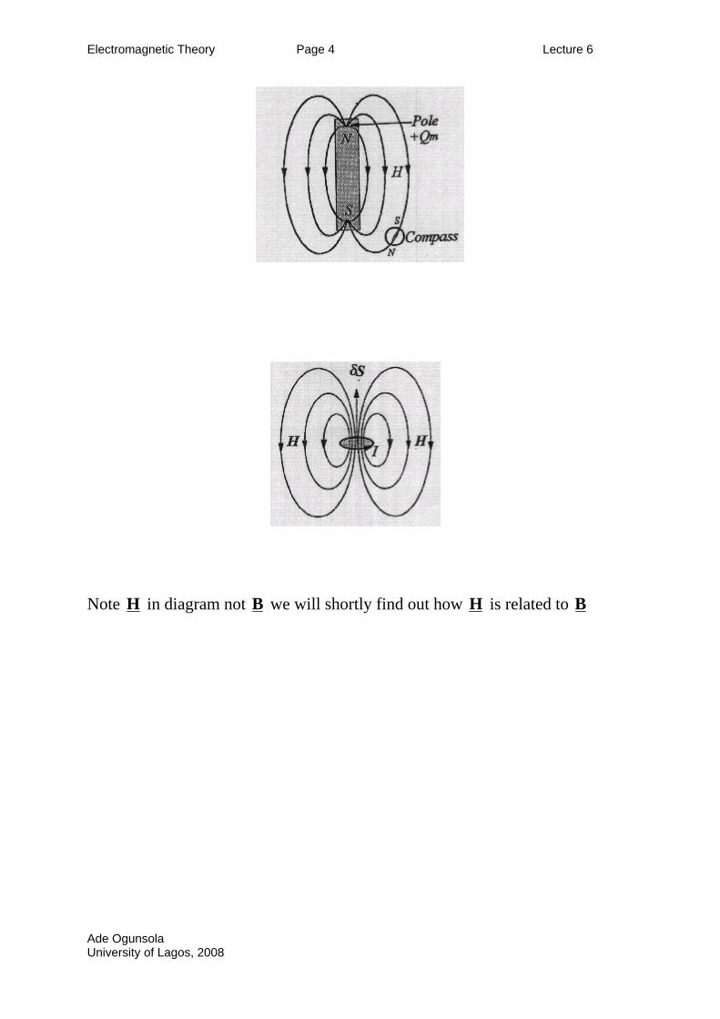
Note H in diagram not B we will shortly find out how H is related to B
Ade Ogunsola University of Lagos, 2008
Electromagnetic Theory Page 5 Lecture 6
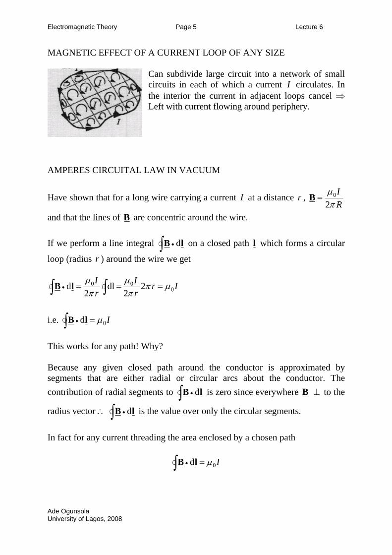
MAGNETIC EFFECT OF A CURRENT LOOP OF ANY SIZE
Can subdivide large circuit into a network of small circuits in each of which a current I circulates. In the interior the current in adjacent loops cancel ⇒ Left with current flowing around periphery.
AMPERES CIRCUITAL LAW IN VACUUM
Have shown that for a long wire carrying a current I at a distance r , RI
πµ2
0=B
and that the lines of B are concentric around the wire. If we perform a line integral ∫ • lB d on a closed path l which forms a circular
loop (radius r ) around the wire we get
IrrI
rI
000 2
2dl
2d µπ
πµ
πµ
=== ∫∫ • lB
i.e. I0d µ=∫ • lB
This works for any path! Why? Because any given closed path around the conductor is approximated by segments that are either radial or circular arcs about the conductor. The contribution of radial segments to ∫ • lB d is zero since everywhere B to the
radius vector ∴
⊥
∫ • lB d is the value over only the circular segments.
In fact for any current threading the area enclosed by a chosen path
I0d µ=∫ • lB
Ade Ogunsola University of Lagos, 2008
Electromagnetic Theory Page 6 Lecture 6
B AND H In a vacuum HB 0µ= =B Magnetic flux density of the magnetic induction [Tesla=NA-1m-1]
=H Magnetic Field [Am-1]
7
0 104 −×= πµ [NA-2 = Tesla A-1m-1] and is called the PERMEABILITY OF FREE SPACE. In vacuum
HB 0µ= ⇒ I=∫ • lH d (A)
Amperes Circuital Law
and ( )34 r
dIl π
rlH ×= ∫ (B)
[ H produced at a distance r from I flowing along path l ] Both (A) and (B) are true in any media. Note: since I=∫ • lH d H field is not conservative unless 0=I .
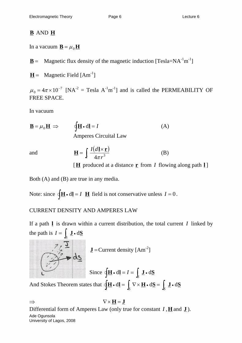
CURRENT DENSITY AND AMPERES LAW If a path l is drawn within a current distribution, the total current I linked by the path is SJ d•∫= S
I
=J Current density [Am-2]
Since SJlH dd •• ∫∫ ==
SI
And Stokes Theorem states that SJSHlH ddd ••• ∫∫∫ =×∇=SSl
⇒ JH =×∇ Differential form of Amperes Law (only true for constant I , H and J ). Ade Ogunsola University of Lagos, 2008
Electromagnetic Theory Page 7 Lecture 6
GAUSS, LAW IN MAGNETISM Magnetic Flux = Total lines of B through a given area.
SB d•∫=ΦS
Remember 0
dεq
S=∫ • SE so in the absence of any charge 0d =∫ •
SSE
Magnetic Monopoles don’t exist – only magnetic dipoles ⇒ 0d =∫ •
SSB always. Since Gauss’ Theorem states
vdv d
S• •∇ =∫ ∫B B S
0d =∫ •
SSB means that 0=∇ • B always.
Lines of B always form closed paths. No sources of B . MAGNETOSTATICS ELECTROSTATICS No charges, no electrical fields. Steady currents and time independent magnetic field.
B , H and J all zero. D and E time independent.
I
l=∫ • lH d
JH =×∇
0=∇ • B
0d =∫ •
llE
0=×∇ E
fρ=∇ • D
Only if 0=J can we define a magnetic scale potential Mφ such that
Mφ−∇=H Note: ( ) 0=∇−×∇=×∇ MφH
V−∇=E
Ade Ogunsola University of Lagos, 2008
Electromagnetic Theory Page 1 Lecture 7
THE MAGNETIC PROPERTIES OF MATERIALS All magnetic materials are affected by the presence of a magnetic field. When a magnetic field of strength H exists within a substance it permeates the material and produces “induced” magnetic dipole throughout the body of the material. The macroscopic measure of this effect is the “MAGNETISATION” M . M IS THE INDUCED MAGNETIC DIPOLE MOMENT PER UNIT VOLUME [Am2m-3 ≡ Am-1] – same units as H . M is the magnetic equivalent of the polarisation P in electrostatics. For simple magnetic media which are linear ( HM ∝ ), homogeneous and isotropic then
HM Mχ= where H is the field strength within the medium and Mχ is the MAGNETIC SUSCEPTIBILITY [Dimensionless]. [In electrostatics EP χε0= where χ is the ELECTRIC SUSCEPTRIBILITY] At room temperature the magnetic susceptibility is typically small and independent of H - BUT for FERROMAGNETIC materials Mχ is large and very dependent on H . DIAMAGNETISM ( )Dχ ,
PARAMAGNETSIM ( )Pχ , and FERROMAGNETISM ( )Fχ
DIAMAGNETISM DIAMAGNETIC substances are composed of atoms (or molecules) that have no permanent magnetic moment. The atom consists of closed shells, so that the magnetic moments associated with individual electron orbitals cancel out and the total angular momentum quantum number 0=J .
It can be shown that e
D m
rZen
6
220µχ −= where is the number of atoms per
unit volume,
n
Z is the number of electrons on each atom, 2r is the average radius of the electron orbital and all other terms have their usual meaning. Note Ade Ogunsola University of Lagos, 2008
Electromagnetic Theory Page 2 Lecture 7
the minus sign, the “INDUCED DIPOLE MOMENT” (or induced current) opposes the applied magnetic flux/field, Dχ is independent of temperature and small in magnitude. Typically for the noble gases (He, Ne Ar, Kr, Xe) with atoms m
ZD10105 −×−≈χ
251069.2 × -3 at RTP. PARAMAGNETISM PARAMAGNETIC substances consist of atoms, ion or molecules that possess a permanent magnetic dipole moment. This atomic electron dipole moment arises from the orbital motion of the electron and the electron spin. The electron magnetic moment of a free atom can be expressed as
Jµ BJg µ=
where ( ) ( )( )12
1123
++−+
+=JJ
LLSSgJ is the Lande g-factor, Am241027.9 −×=Bµ-2
is the Bohr Magneton, and SLJ += is the “Effective spin” angular momentum. In the absence of an applied magnetic field the directions of the magnetic dipole moments (µ ) of the individual atoms are randomised by thermal energy and the net magnetic moment of a macroscopic volume is zero. When B is applied dipole tend to align themselves in the direction of the field – Magnetic alignment energy Bµ •−= . If TkB<<• Bµ then the result is a small net alignment in the direction of the field – induced magnetic moment is in the same direction as the applied B ⇒ 0>Pχ (positive!). It the atoms/molecules/ions are sufficiently far apart that their mutual interactions can be neglected (i.e. gas of low concentration of paramagnetic ions in a diamagnetic solid) then
TC
Tkn
BP ==
3
20 µµχ if TkB<<• Bµ
=n Number of atoms/molecules/ions per unit volume ( )1222 += JJg BJµµ
=C Curie Constant Note Pχ is positive, small and depends on temperature as T
1 . For solids and liquids where interactions between paramagnetic atoms/ions cannot be neglected
θχ
−≈
TC
P Only works for θ>T
=C Constant, =θ Weiss constant can be positive or negative.
Ade Ogunsola University of Lagos, 2008
Electromagnetic Theory Page 3 Lecture 7
FERROMAGNETSIM Ferromagnetic substances are all solid, and each is characterised by a certain temperature known as the CURIE POINT at which the properties change abruptly.
• Magnetisation is not proportional to H , in certain situations a susceptibility of several thousand an be measured and very large magnetisations can be achieved.
• The value of the magnetisation depends not only on the applied field but also on the previous history of the samples.
• A sample may retain its magnetisation even in the absence of an external applied field – PERMANENT MAGNETS. However, it is notable that the very same material can also exist is a state showing little or no permanent magnetism.
The ultimate source of magnetic moments in ferromagnetic materials turns out to be the magnetic moments arising from electron spin – the big difference in Ferromagnetics (cf. Paramagnetism) is that there are large interactions between spins that cause them to align parallel with each other – even at room temperature thermal vibrations cannot destroy the alignment.
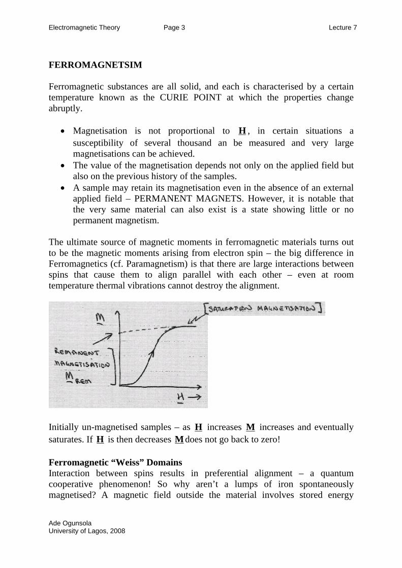
Initially un-magnetised samples – as H increases M increases and eventually saturates. If H is then decreases M does not go back to zero! Ferromagnetic “Weiss” Domains Interaction between spins results in preferential alignment – a quantum cooperative phenomenon! So why aren’t a lumps of iron spontaneously magnetised? A magnetic field outside the material involves stored energy
Ade Ogunsola University of Lagos, 2008
Electromagnetic Theory Page 4 Lecture 7
∫ •=v
dv21 BH [J]. If the sample is “broken up” into differently oriented
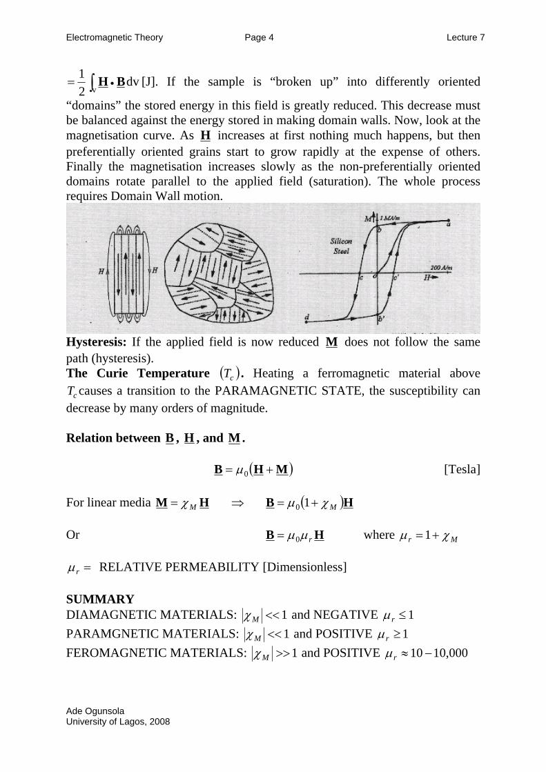
“domains” the stored energy in this field is greatly reduced. This decrease must be balanced against the energy stored in making domain walls. Now, look at the magnetisation curve. As H increases at first nothing much happens, but then preferentially oriented grains start to grow rapidly at the expense of others. Finally the magnetisation increases slowly as the non-preferentially oriented domains rotate parallel to the applied field (saturation). The whole process requires Domain Wall motion.
Hysteresis: If the applied field is now reduced M does not follow the same path (hysteresis). The Curie Temperature ( ) . Heating a ferromagnetic material above
causes a transition to the PARAMAGNETIC STATE, the susceptibility can decrease by many orders of magnitude.
cTcT
Relation between B , H , and M .
( )MHB += 0µ [Tesla]
For linear media HM Mχ= ⇒ ( )HB Mχµ += 10 Or HB rµµ0= where Mr χµ +=1
=rµ RELATIVE PERMEABILITY [Dimensionless] SUMMARY DIAMAGNETIC MATERIALS: 1<<Mχ and NEGATIVE 1≤rµ PARAMGNETIC MATERIALS: 1<<Mχ and POSITIVE 1≥rµ FEROMAGNETIC MATERIALS: 1>>Mχ and POSITIVE 000,1010 −≈rµ
Ade Ogunsola University of Lagos, 2008
Electromagnetic Theory Page 1 Lecture 8
BOUNDARY CONDITIONS IN MAGNETISM We will consider boundaries between linear, isotropic and homogeneous media. THE TANGENTIAL COMPONENT OF H IS CONTINUOUS
ACROSS A BOUNDARY PROVIDED THAT THERE IS NO SURFACE CURRENT ON THE BOUNDARY.
THE NORMAL COMPONENT OF B IS CONTINUOUS ACROSS A
BOUNDARY.
ANY SOLUTION TO AN MAGNETOSTATICS PROBLEM MUST SATISFY THE BOUNDARY CONDITIONS.
THE TANGENTIAL COMPONENT OF H
H2
H1
Region 1 µr1
Region 2 µr2
C
DA
B
⊗
⊗
⊗
⊗ ⊗
⊗ ⊗ ⊗ ⊗ ⊗ ⊗
⊗ ⊗ ⊗
∆x
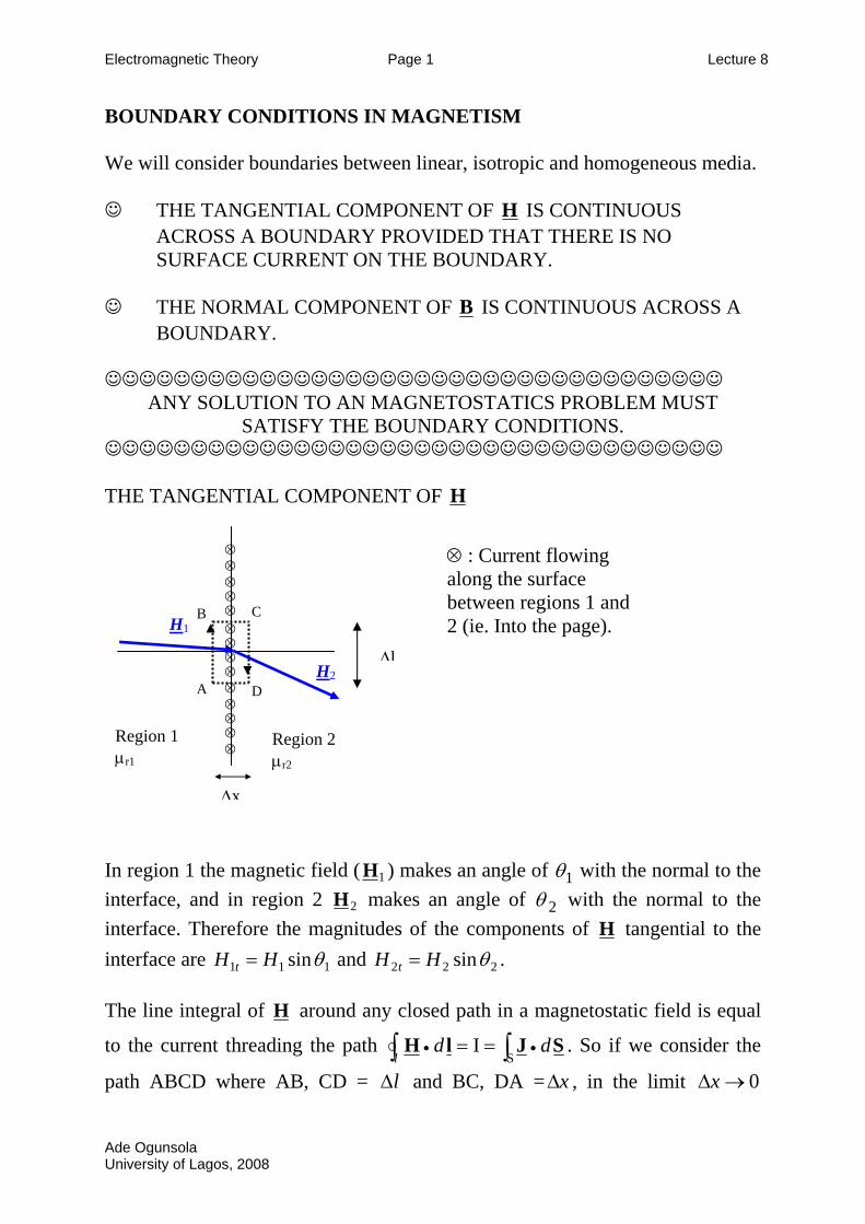
⊗ : Current flowing along the surface between regions 1 and 2 (ie. Into the page).
∆l In region 1 the magnetic field ( 1H ) makes an angle of 1θ with the normal to the interface, and in region 2 2H makes an angle of 2θ with the normal to the interface. Therefore the magnitudes of the components of H tangential to the interface are 111 sinθHH t = and 222 sinθHH t = . The line integral of H around any closed path in a magnetostatic field is equal
to the current threading the path ∫∫ •• ==S
I SJlH ddl
. So if we consider the
path ABCD where AB, CD = l∆ and BC, DA = x∆ , in the limit 0→∆x
Ade Ogunsola University of Lagos, 2008
Electromagnetic Theory Page 2 Lecture 8
∫ →•S
0SJ d since current density is finite in everything except a perfect conductor.
021 =∆−∆=∫ • lHlHd ttllH
∴ 021 =− tt HH then tt HH 21 = (Tangential component of H is continuous across a boundary)
Because HB rµµ0= 1
1
2
2
µµtt BB
=
i.e. The tangential component of B is discontinuous as the boundary. (Aside: For a perfect conductor can consider a surface charge per unit length
flowing in a vanishing thin layer at the interface, then the boundary condition becomes )
SjStt jHH =− 21
THE NORMAL COMPONENT OF B
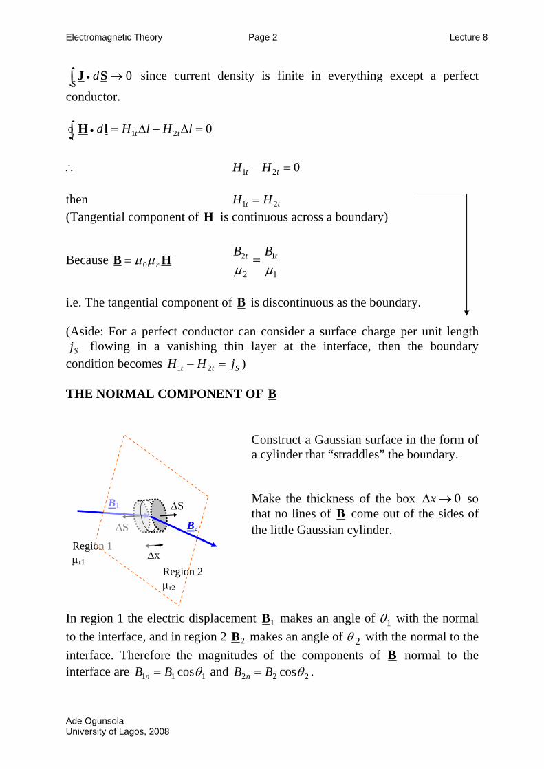
Construct a Gaussian surface in the form of a cylinder that “straddles” the boundary.
B1
Region 1 µr1
∆S B2
Region 2 µr2
∆x
∆S
Make the thickness of the box 0→∆x so that no lines of B come out of the sides of the little Gaussian cylinder.
In region 1 the electric displacement 1B makes an angle of 1θ with the normal to the interface, and in region 2 2B makes an angle of 2θ with the normal to the interface. Therefore the magnitudes of the components of B normal to the interface are 111 cosθBB n = and 222 cosθBB n = .
Ade Ogunsola University of Lagos, 2008
Electromagnetic Theory Page 3 Lecture 8
Since 0d =∫ • SBS
then SBSB ∫∫ •• −=21
ddSS
SBSB nn ∆=∆ 12
∴ nn BB 21 =
Because HB rµµ0= there is a “jump” in the normal component of the magnetic field at the boundary.
nn HH 1122 µµ = REFRACTION OF LINES OF B AND H .
Boundary conditions: 0=Sj tt HH 21 = or
0=Sj 2211 sinsin θθ HH =
and nn BB 12 = or 2211 coscos θθ BB =
So 22
21
1
1 cotcot θθHB
HB
= and since HB rµµ0= we find that
2211 cotcot θµθµ = : Refraction formula for magnetic field lines.
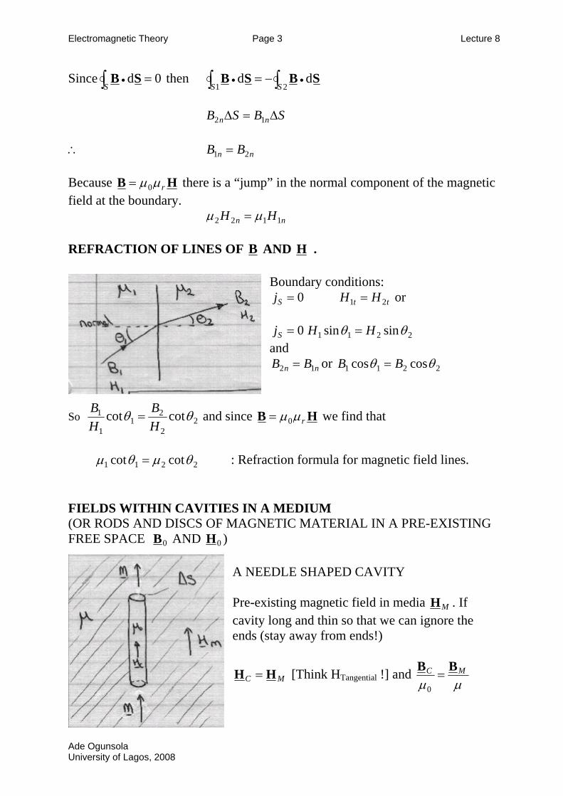
FIELDS WITHIN CAVITIES IN A MEDIUM (OR RODS AND DISCS OF MAGNETIC MATERIAL IN A PRE-EXISTING FREE SPACE 0B AND 0H )
A NEEDLE SHAPED CAVITY Pre-existing magnetic field in media MH . If cavity long and thin so that we can ignore the ends (stay away from ends!)
MC HH = [Think HTangential !] and µµMC BB
=0
Ade Ogunsola University of Lagos, 2008
Electromagnetic Theory Page 4 Lecture 8
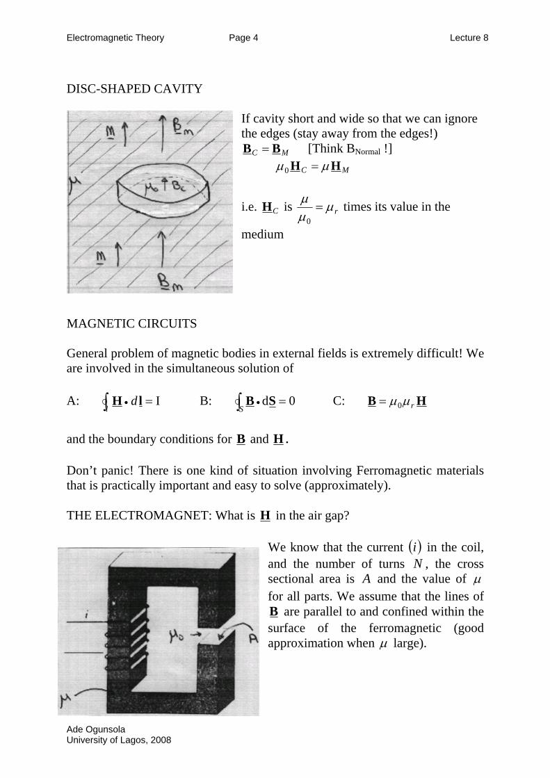
DISC-SHAPED CAVITY
If cavity short and wide so that we can ignore the edges (stay away from the edges!)
MC BB = [Think BNormal !] MC HH µµ =0
i.e. CH is rµµµ
=0
times its value in the
medium
MAGNETIC CIRCUITS General problem of magnetic bodies in external fields is extremely difficult! We are involved in the simultaneous solution of A: I=∫ •
ld lH B: 0d =∫ • SB
S C: HB rµµ0=
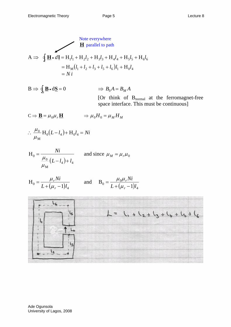
and the boundary conditions for B and H . Don’t panic! There is one kind of situation involving Ferromagnetic materials that is practically important and easy to solve (approximately). THE ELECTROMAGNET: What is H in the air gap?
We know that the current ( in the coil, and the number of turns
)iN , the cross
sectional area is A and the value of µ for all parts. We assume that the lines of B are parallel to and confined within the surface of the ferromagnetic (good approximation when µ large).
Ade Ogunsola University of Lagos, 2008
Electromagnetic Theory Page 5 Lecture 8
Note everywhere
H parallel to path A ⇒ 665544332211 HHHHHH lllllld
l+++++=∫ • lH
( ) 40165321M HH lllllll +++++= iN=
B ⇒ 0d =∫ • SB
S ⇒ ABAB M=0
[Or think of Bnormal at the ferromagnet-free space interface. This must be continuous]
C ⇒ HB rµµ0= ⇒ MM HH µµ =00
∴ ( ) NillL =+− 4040M
0 HHµµ
( ) 44M
00H
llL
Ni
+−=
µµ and since 0µµµ rM =
( ) 40 1
HlL
Ni
r
r
−+=
µµ and ( ) 4
00 1
BlL
Ni
r
r
−+=
µµµ
Ade Ogunsola University of Lagos, 2008
Electromagnetic Theory Page 1 Lecture 9
MAXWELLS EQUATIONS GAUSS’ LAW (i) ELECTROSTATICS
∫∫ ==•v
vdQdS
ρSD or ρ=∇ • D
=D Electric Displacement [Cm-2]
(i) MAGNETOSTATICS
0=∫ •S
dSB or 0=∇ • B =B Magnetic Flux Density [Tesla]
AMPERES CIRCUITAL LAW
SJlH dd •• ∫∫ ==Sl
I or JH =×∇
=H Magnetic Field [Am-1] =J Current density [Am-2]
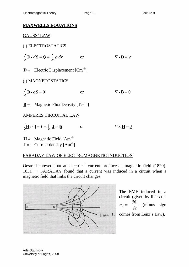
FARADAY LAW OF ELECTROMAGNETIC INDUCTION Oestred showed that an electrical current produces a magnetic field (1820). 1831 ⇒ FARADAY found that a current was induced in a circuit when a magnetic field that links the circuit changes.
The EMF induced in a circuit (given by line l) is
tV ∂Φ∂
−=ε (minus sign
comes from Lenz’s Law).
Ade Ogunsola University of Lagos, 2008
Electromagnetic Theory Page 2 Lecture 9
∫ •=ΦS
dSB (Any surface whose boundary is the line l)
=Φ MAGNETIC FLUX linked by the circuit [Tesla m2 or Weber, Wb] The induced EMF Vε is equal the line integral of the induced E [Vm-1] electric field around the coil.
∫∫ ••∂∂
−=∂Φ∂
−=Sl
dtt
SBlE d
Using Stokes Theorem SElE dd •• ∫∫ ×∇=
Sl
∫∫ ••∂∂
−=×∇SS
dt
SBSE d
∴ t∂
∂−=×∇
BE
CONSTITUTIVE RELATIONS
Ohms Law IRV = , A
lR Rρ= =Rρ Resistivity [Ωm]
RC ρ
σ 1= =Cσ Conductivity [ 1−Ω m-1]
AlV
lAV
RVI C
Rσ
ρ=== , re-arrange and we get EJ
AI
Cσ==
Or in vector form (Homogeneous, isotropic media) EJ Cσ= So we now have:
PED += 0ε ED rεε0=
( MHB += 0 )µ HB rµµ0=
EJ Cσ=
Ade Ogunsola University of Lagos, 2008
Electromagnetic Theory Page 3 Lecture 9
POWER DISSIPATION AND JOULE HEATING Power is dissipated in the resistance R causing “Joule Heating”.
RIR
VIVW 22
===
][22 VolumeEJlAEJA
lAJWC
C
C×===
σσ
σ
dv
vEJ •∫=W [Now works if E and J in different directions
and/or vary with position] THE EQUATION OF CONTINUITY
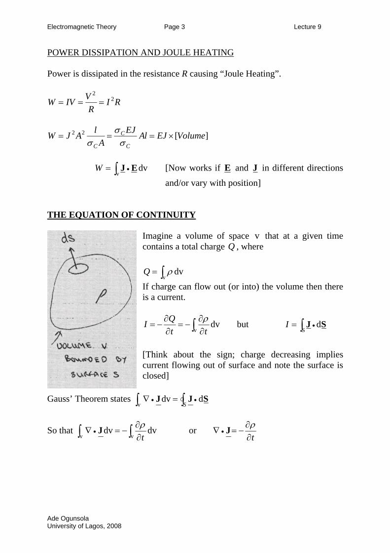
Imagine a volume of space v that at a given time contains a total charge Q , where
∫= vdvρQ
If charge can flow out (or into) the volume then there is a current.
∫ ∂∂
−=∂∂
−=v
dvtt
QI ρ but ∫ •=S
dSJI
[Think about the sign; charge decreasing implies current flowing out of surface and note the surface is closed]
Gauss’ Theorem states ∫∫ •• =∇S
SJJ ddvv
So that ∫∫ ∂∂
−=∇ •vv
dvdvtρJ or
t∂∂
−=∇ •ρJ
Ade Ogunsola University of Lagos, 2008
Electromagnetic Theory Page 4 Lecture 9
DISPLACEMENT CURRENT In magnetostatics we found that I
l=∫ • lH d and hence JH =×∇
But 0=×∇•∇ H always (!) and 0≠∇ • J always!
0=∇ • J only when 0=∂∂
tρ i.e. STATICS
RESOLUTION OF THE PROBLEM
ρ=∇ • D ⇒ tt ∂
∂=
∂∂
∇ •ρD
As t∂
∂−=∇ •
ρJ ⇒ t∂
∂−∇=∇ ••
DJ or 0=⎟⎟⎠
⎞⎜⎜⎝
⎛∂∂
+∇ •tDJ
Now we can see how we may amend Amperes Law t∂
∂+=×∇
DJH
=∂∂
tD Displacement current density [Am-2]
Total effective current t∂
∂+=
DJ [Am-2]
=J Conduction current density [Am-2]
∫ •=S
dSJI Conduction Current
∫ •∂∂
=S
dSDt
I Displacement Current (not a real current)
Ade Ogunsola University of Lagos, 2008
Electromagnetic Theory Page 5 Lecture 9
AMPERE-MAXWELL LAW IN A DIELECTRIC WITH A FINTE CONDUCTIVITY
t∂∂
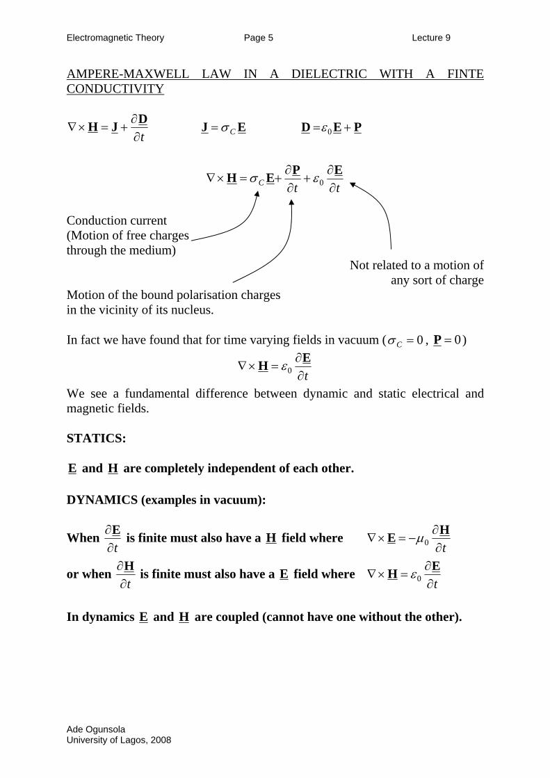
+=×∇DJH EJ Cσ= PED += 0ε
ttC ∂∂
+∂∂
+=×∇EPEH 0εσ
Conduction current (Motion of free charges through the medium)
Not related to a motion of any sort of charge
Motion of the bound polarisation charges in the vicinity of its nucleus. In fact we have found that for time varying fields in vacuum ( 0=Cσ , 0=P )
t∂∂
=×∇EH 0ε
We see a fundamental difference between dynamic and static electrical and magnetic fields. STATICS: E and H are completely independent of each other.
DYNAMICS (examples in vacuum):
When t∂
∂E is finite must also have a H field where t∂
∂−=×∇
HE 0µ
or when t∂
∂H is finite must also have a E field where t∂
∂=×∇
EH 0ε
In dynamics E and H are coupled (cannot have one without the other).
Ade Ogunsola University of Lagos, 2008
Electromagnetic Theory Page 6 Lecture 9
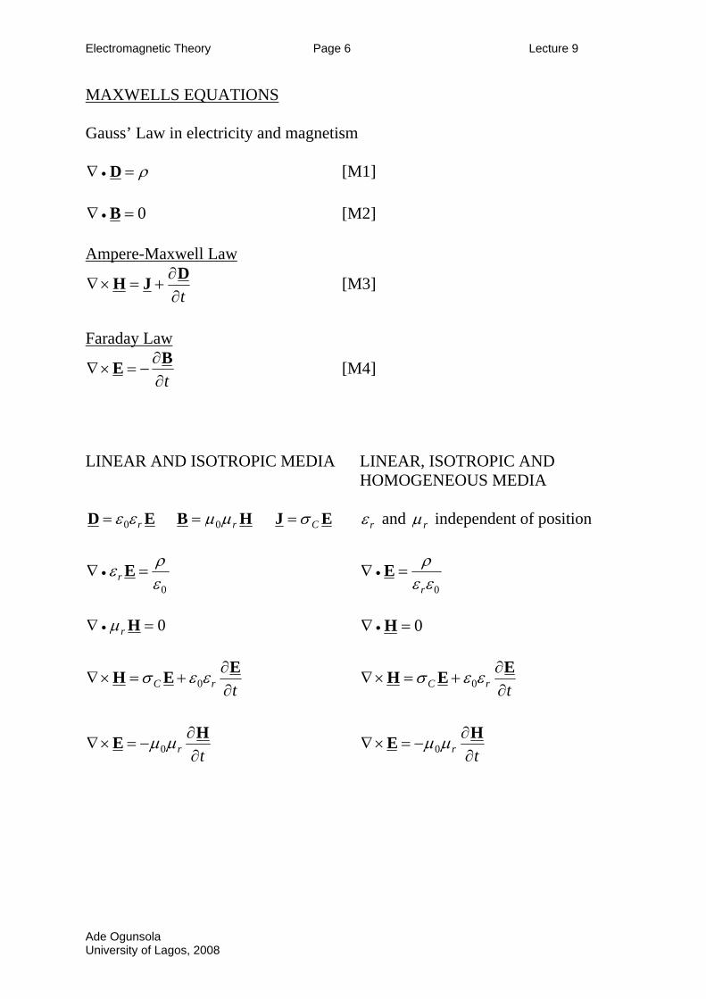
MAXWELLS EQUATIONS Gauss’ Law in electricity and magnetism
ρ=∇ • D [M1]
0=∇ • B [M2] Ampere-Maxwell Law
t∂∂
+=×∇DJH [M3]
Faraday Law
t∂∂
−=×∇BE [M4]
LINEAR AND ISOTROPIC MEDIA LINEAR, ISOTROPIC AND
HOMOGENEOUS MEDIA
ED rεε0= HB rµµ0= EJ Cσ=
rε and rµ independent of position
0ερε =∇ • Er
0εε
ρ
r=∇ • E
0=∇ • Hrµ
0=∇ • H
trC ∂∂
+=×∇EEH εεσ 0
trC ∂
∂+=×∇
EEH εεσ 0
tr ∂∂
−=×∇HE µµ0
tr ∂
∂−=×∇
HE µµ0
Ade Ogunsola University of Lagos, 2008
Electromagnetic Theory Page 1 Lecture 10
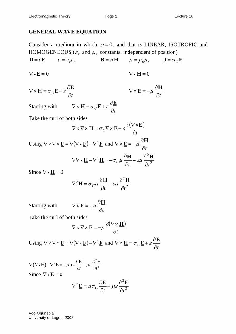
GENERAL WAVE EQUATION Consider a medium in which 0=ρ , and that is LINEAR, ISOTROPIC and HOMOGENEOUS ( rε and rµ constants, independent of position)
ED ε= rεεε 0= HB µ= rµµµ 0= EJ Cσ=
0=∇ • E 0=∇ • H
tC ∂∂
+=×∇EEH εσ
t∂∂
−=×∇HE µ
Starting with tC ∂
∂+=×∇
EEH εσ
Take the curl of both sides ( )
tC ∂×∇∂
+×∇=×∇×∇EEH εσ
Using ( ) FFF 2∇−∇∇=×∇×∇ • and t∂
∂−=×∇
HE µ
2
22
ttC ∂∂
−∂∂
−=∇−∇∇ •HHHH εµµσ
Since 0=∇ • H
2
22
ttC ∂∂
+∂∂
=∇HHH εµµσ
Starting with t∂
∂−=×∇
HE µ
Take the curl of both sides
( )t∂×∇∂
−=×∇×∇HE µ
Using ( ) FFF 2∇−∇∇=×∇×∇ • and tC ∂
∂+=×∇
EEH εσ
( )2
22C t t
µσ µε•∂ ∂
∇ ∇ −∇ = − −∂ ∂E EE E
Since 0=∇ • E
2
22
ttC ∂∂
+∂∂
=∇EEE µεµσ
Ade Ogunsola University of Lagos, 2008
Electromagnetic Theory Page 2 Lecture 10
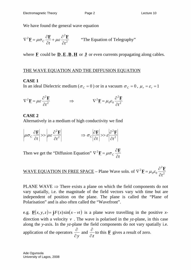
We have found the general wave equation
2
22
ttC ∂∂
+∂∂
=∇FFF µεµσ “The Equation of Telegraphy”
where F could be D ,E ,B , H or J or even currents propagating along cables. THE WAVE EQUATION AND THE DIFFUSION EQUATION CASE 1 In an ideal Dielectric medium ( 0=Cσ ) or in a vacuum 0=Cσ , 1== rr εµ
2
22
t∂∂
=∇FF µε ⇒ 2
2
002
t∂∂
=∇FF εµ
CASE 2 Alternatively in a medium of high conductivity we find
2
2
ttC ∂∂
>>∂∂ FF µεµσ ⇒ 2
2
ttC ∂∂
>>∂∂ FF εσ
Then we get the “Diffusion Equation” tC ∂
∂=∇
FF µσ2
WAVE EQUATION IN FREE SPACE – Plane Wave soln. of 2
2
002
t∂∂
=∇FF εµ
PLANE WAVE ⇒ There exists a plane on which the field components do not vary spatially, i.e. the magnitude of the field vectors vary with time but are independent of position on the plane. The plane is called the “Plane of Polarisation” and is also often called the “Wavefront”. e.g. ( ) ( vtxxFzyx −= sin)(,, jF ) is a plane wave travelling in the positive x-direction with a velocity . The wave is polarised in the yz-plane, in this case along the y-axis. In the yz-plane the field components do not vary spatially i.e.
application of the operators
v
y∂∂ and
z∂∂ to this F gives a result of zero.
Ade Ogunsola University of Lagos, 2008
Electromagnetic Theory Page 3 Lecture 10
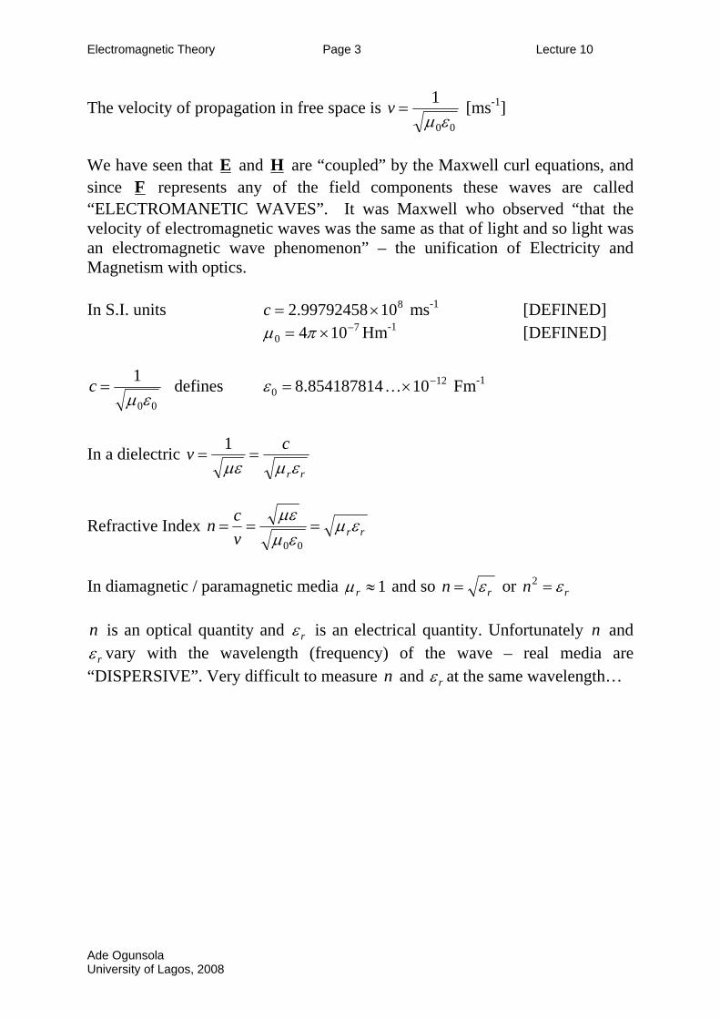
The velocity of propagation in free space is 00
1εµ
=v [ms-1]
We have seen that E and H are “coupled” by the Maxwell curl equations, and since F represents any of the field components these waves are called “ELECTROMANETIC WAVES”. It was Maxwell who observed “that the velocity of electromagnetic waves was the same as that of light and so light was an electromagnetic wave phenomenon” – the unification of Electricity and Magnetism with optics. In S.I. units 81099792458.2 ×=c ms-1 [DEFINED] Hm7
0 104 −×= πµ -1 [DEFINED]
00
1εµ
=c defines Fm120 10854187814.8 −×= …ε -1
In a dielectric rr
cvεµµε
==1
Refractive Index rrvcn εµ
εµµε
===00
In diamagnetic / paramagnetic media 1≈rµ and so rn ε= or rn ε=2
n is an optical quantity and rε is an electrical quantity. Unfortunately and n
rε vary with the wavelength (frequency) of the wave – real media are “DISPERSIVE”. Very difficult to measure and n rε at the same wavelength…
Ade Ogunsola University of Lagos, 2008
Electromagnetic Theory Page 4 Lecture 10
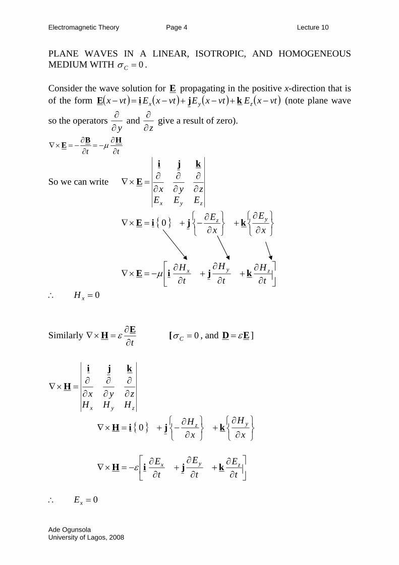
PLANE WAVES IN A LINEAR, ISOTROPIC, AND HOMOGENEOUS MEDIUM WITH 0=Cσ . Consider the wave solution for E propagating in the positive x-direction that is of the form ( ) ( ) ( ) ( )vtxEvtxEvtxEvtx zyx −+−+−=− kjiE (note plane wave
so the operators y∂∂ and
z∂∂ give a result of zero).
t tµ∂ ∂
∇× = − = −∂ ∂B HE
So we can write
zyx EEEzyx ∂∂
∂∂
∂∂=×∇
kji
E
⎭⎬⎫
⎩⎨⎧∂
∂+
⎭⎬⎫
⎩⎨⎧
∂∂
−+=×∇x
Ex
E yz kjiE 0
⎥⎦
⎤⎢⎣
⎡∂∂
+∂
∂+
∂∂
−=×∇t
Ht
Ht
H zyx kjiE µ
∴ 0=xH
Similarly t∂
∂=×∇
EH ε [ 0=Cσ , and ED ε= ]
zyx HHHzyx ∂∂
∂∂
∂∂
=×∇
kji
H
⎭⎬⎫
⎩⎨⎧∂
∂+
⎭⎬⎫
⎩⎨⎧
∂∂
−+=×∇x
Hx
H yz kjiH 0
⎥⎦
⎤⎢⎣
⎡∂∂
+∂
∂+
∂∂
−=×∇t
Et
Et
E zyx kjiH ε
∴ 0=xE
Ade Ogunsola University of Lagos, 2008
Electromagnetic Theory Page 5 Lecture 10
∴ In a linear, isotropic medium where rε and rµ are scalar constants so that be “ D and E ” and “B and H ” are parallel. No component of the wave field is in the x-direction. All wave components lie in the plane of the wavefront, transverse (perpendicular) to the direction of propagation. Plane electromagnetic waves are a TRANSVERSE wave motion in an “isotropic” medium – called TEM mode (no longitudinal component of the electromagnetic field. From y-components (top line) and z-components (second line)
tE
xH
tH
xE
tE
xH
tH
xE
zyzy
yzyz
∂∂
=∂
∂
∂∂
−=∂
∂
∂∂
=∂∂
−∂∂
=∂∂
εµ
εµ
and
and
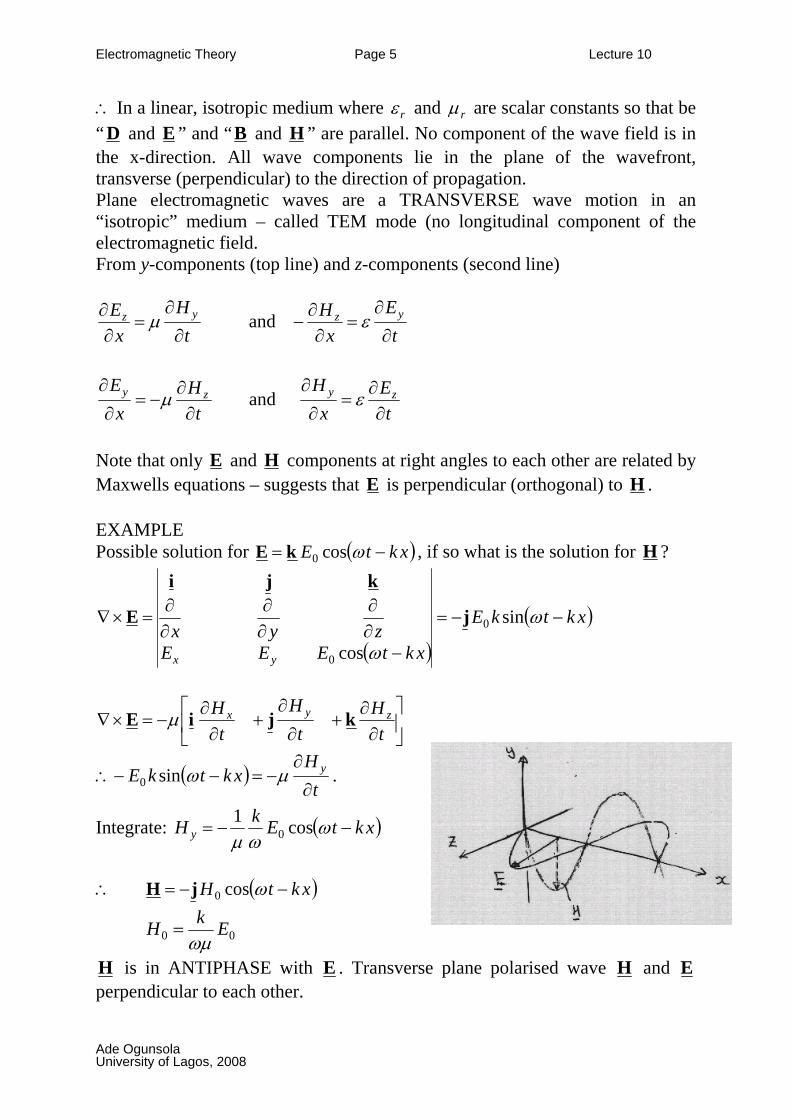
Note that only E and H components at right angles to each other are related by Maxwells equations – suggests that E is perpendicular (orthogonal) to H . EXAMPLE Possible solution for ( )xktE −= ωcos0kE , if so what is the solution for H ?
( )( )xktkE
xktEEEzyx
yx
−−=
−∂∂
∂∂
∂∂
=×∇ ω
ω
sin
cos
0
0
j
kji
E
⎥⎦
⎤⎢⎣
⎡∂∂
+∂
∂+
∂∂
−=×∇t
Ht
Ht
H zyx kjiE µ
∴ ( )t
HxktkE y
∂
∂−=−− µωsin0 .
Integrate: ( )xktEkH y −−= ωωµ
cos10
∴ ( )xktH −−= ωcos0jH
00 EkHωµ
=
H is in ANTIPHASE with E . Transverse plane polarised wave H and E perpendicular to each other.
Ade Ogunsola University of Lagos, 2008
Electromagnetic Theory Page 1 Lecture 11
THE COMPLEX REPRESENTATION OF ELECTROMAGNETIC WAVES We discovered in the last lecture that we had to solve equations of the form
2
22
ttC ∂∂
+∂∂
=∇EEE µεµσ
The solution to this equation can be written in the complex form
( ) ( ) ( )tjzyxtzyx ωexp,,~,,, EE = In general ( zyx ,, )~E is a complex number (vector) that varies spatially but is independent of time.
== fπω 2 Angular wave Frequency [Rad s-1], and =f Wave Frequency [Hz]
Note EE ωjt=
∂∂ and EE 2
2
2
ω−=∂∂
t
Remember physical “wave fields” are REAL functions of position and time. When solving a problem we must recover the “real part” from the solution – note this is not as obvious as it may seem because ( )zyx ,,~E can be a complex number. Using the complex notation the wave equation becomes
EEE 22 µεωµσω −=∇ Cj Remember we could replace E with D , B , H or J and the equation would still be valid.
Ade Ogunsola University of Lagos, 2008
Electromagnetic Theory Page 2 Lecture 11
THE SINGLE PROGRESSIVE (COMPLEX) PLANE WAVE IN AN IDEAL DIELECTRIC ( 0=Cσ ). Must find a solution for E that satisfies the equation EE µεω 22 −=∇ COHERNET
TIME HARMONIC WAVE
Assume the solution is of the form ( ) ( )[ ]xktjtzyx −= ωexp~,,, 0EE Amplitude of the wave oscillation (Complex Constant) k is called the spatial frequency or wavenumber. jk is called the propagation constant.
kx−=φ is the phase of the wave (so in any plane =x constant is a plane of
constant phase).
EEE 22
22 k
x−=
∂∂
=∇ and EE 22
2
ω−=∂∂
t
∴ EE 22 µεω−=− k and hence cn
vk ω
λπωµεω ±=±=±=±=
2
• =k positive root ⇒ Wave propagating in the positive x-direction. • µεω±=k which is a real number – peak amplitude does not change as
wave propagates in the x-direction. Wave is said to be “un-attenuated”.
Ade Ogunsola University of Lagos, 2008
Electromagnetic Theory Page 3 Lecture 11
THE PHYSICAL SOLUTION – we want the real part of ( )zyx ,,~E subject to the appropriate boundary conditions. We have ( ) ( )[ xktjtzyx −= ωexp ]~,,, 0EE but we know that there is no wave component of the electric field in the x-direction. ∴ ( ) ( ) ( )[ ]xktjEEtzyx zy −+= ωexp~~,,, 00 kjE Example 1 If 00
~yy EE = and 00
~zz EE = (both and are real constants) 0yE 0zE
Then ( ) ( ) ( )xktEEtzyx zy −+= ωcos,,, 00 kjE Example 2 If 00
~yy jEE −= and (both and are real constants) 00
~zz jEE −= 0yE 0zE
Then ( ) ( ) ( )xktEEtzyx zy −+= ωsin,,, 00 kjE Example 3 If 00
~yy jEE −= and 00
~z
jz EjeE δ−= ( , and 0yE 0zE δ are real constants)
Then ( ) ( ) ( )δωω +−+−= xktExktEtzyx zy sinsin,,, 00 kjE The z-component leads the y-component by the phase angle zE yE δ .
Ade Ogunsola University of Lagos, 2008
Electromagnetic Theory Page 4 Lecture 11
Now we have the electric field component, how do we get the magnetic field component?
t∂∂
=×∇EH ε
t∂∂
−=×∇HE µ
zy EEzyx
~~0∂∂
∂∂
∂∂
=×∇
kji
E
( )[ ]( ) ( )[ ]( )⎭⎬⎫
⎩⎨⎧
−∂∂
+⎭⎬⎫
⎩⎨⎧
−∂∂
−+=×∇ xktjEx
xktjEx yz ωω exp~exp~0 00 kjiE
( )[ ]( ) ( )[ ]( ) ( )[ ]( )xktjHt
xktjHt
xktjHtt zyx −
∂∂
+−∂∂
+−∂∂
=∂∂ ωωω exp~exp~exp~
000 kjiH
t∂∂
−=×∇HE µ
⇒ 0~
0 =xH
⇒ 00~~
yz HjEjk ωµ−= and hence 00~~
zy EkHµω
−=
⇒ 00~~
zy HjEjk ωµ−=− and hence 00~~
yz EkHµω
=
( ) ( )[ ]xktjEkEktzyx yz −⎟⎟⎠
⎞⎜⎜⎝
⎛⎟⎟⎠
⎞⎜⎜⎝
⎛+⎟⎟
⎠
⎞⎜⎜⎝
⎛−= ω
µωµωexp~~,,, 00 kjH
( ) ( ) ( )[ ]xktjHHtzyx zy −+= ωexp~~,,, 00 kjH
Ade Ogunsola University of Lagos, 2008
Electromagnetic Theory Page 5 Lecture 11
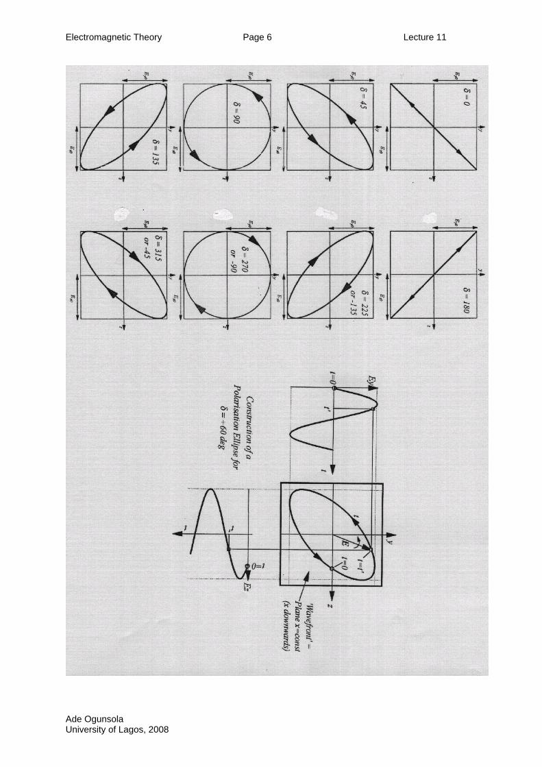
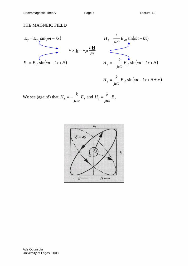
THE POLARISATION STATE OF AN ELECTROMAGNETIC WAVE Consider the wave with ( ) ( )δωω +−+−= xktExktE zy sinsin 00 kjE i.e. ( xktEE yy )−= ωsin0 and ( )δω +−= xktEE zz sin0 Various polarisation sates of the wave are possible depending on the relative magnitudes and phases of the two “E” components. Consider any plane x=constant. Any such plane of constant phase and is called a “plane of polarisation” or a “wavefront”. What happens in this plane as time varies? Consider the plane x=0. ( )tEE yy ωsin0= and ( )δω += tEE zz sin0 • If 0=δ or πδ = , the polarisation is LINEAR. The amplitude of the total
electric vector varies between zero and 20
20 zy EEE += .
• If 2πδ ±= and the polarisation is CIRCULAR and the magnitude
of the total electric vector is independent of time. 00 zy EE =
• If πδ <<0 figure s described in an “anticlockwise” sense. • If 0<<− δπ figure s described in a “clockwise” sense. • Otherwise the polarisation of the wave is elliptical. The magnitude of the
total electric vector is never zero.
Ade Ogunsola University of Lagos, 2008
Electromagnetic Theory Page 6 Lecture 11
Ade Ogunsola University of Lagos, 2008
Electromagnetic Theory Page 7 Lecture 11
THE MAGNEIC FIELD
( kxtEE yy −= )ωsin0 ( )kxtEkH yz −= ωµω
sin0
t∂
∂−=×∇
HE µ
( )δω +−= kxtEE zz sin0 ( )δωµω
+−−= kxtEkH zy sin0
( )πδωµω
±+−= kxtEkH zy sin0
We see (again!) that zy EkHµω
−= and yz EkHµω
=
Ade Ogunsola University of Lagos, 2008
Electromagnetic Theory Page 8 Lecture 11
ORTHOGONALITY 0=++=• zzyyxx HEHEHEHE E and H are perpendicular to each other at all times! WAVE IMPEDANCE/ INTRINSIC IMPEDANCE OF A MEDIUM
( )kxtEE yy −= ωsin0 and ( )δω +−= kxtEE zz sin0 The magnitude of the electric field is 22
zy EEE +=
Similarly EEEEkHHH yzzy µε
µωωεµ
µω==+=+= 2222
∴ εµ
=HE [Ohm] INTRISIC IMPEDANCE OF THE MEDIUM
In free space Ω== 3770
0
εµ
HE . In an ideal dielectric
r
r
HE
εµ
εµ
0
0= (real
quantity purely resistive)
[Note: r
r
HE
εµ
εµ
0
0= and ED ε= so HD µε= etc.]
ENERGY TRANSPORTED IN EM-WAVE
εµ
=HE ⇒ 2
02
0 HE rr µµεε =
=2
20 Erεε ENERGY DENSITY OF ELECTRIC FIELD [Jm-3]
=2
20 Hrεε ENERGY DENSITY OF MAGNETIC FIELD [Jm-3]
2
02
0 HE rr µµεε = ⇒Wave energy is equally divided between electric and magnetic components of field in dielectric medium.
Ade Ogunsola University of Lagos, 2008
Electromagnetic Theory Page 1 Lecture 12
ELECTROMAGNETIC WAVES IN MEDIA OF FINITE CONDUCTIVITY. Relaxation Time of the Medium Linear, homogeneous, isotropic medium of conductivity cσ which contains free charge of volume density ρ
Equation of continuity 0=∂∂
+∇ •tρJ
EJ Cσ= ⇒ ECtσρ
•−∇=∂∂
ED ε= ⇒ D•∇−=∂∂
εσρ C
t
ρ=∇ • D ⇒ ρεσρ C
t−=
∂∂ or 0=+
∂∂ ρ
εσρ C
t
Solution of which is ( ) ( ) ⎟⎠⎞
⎜⎝⎛−=
τρρ tzyxtzyx exp,,,,, where
Cσετ = and is
called the “relaxation time”. e.g. For copper and 117108.5 −−Ω×= mcσ 1≈rε so that 1810−≈τ s
For pure water and 11510 −−− Ω≈ mcσ 80≈rε so that 610−≈τ s ∴ If a free charge density is present in a conducting medium, it decays away at a rate that is independent of any applied fields. ⇒ Eventually all the free charge resides on the surface of the medium – A well know result in Electrostatics of Conductors! It is impossible to create a stable free charge distribution in a conducting medium.
Ade Ogunsola University of Lagos, 2008
Electromagnetic Theory Page 2 Lecture 12
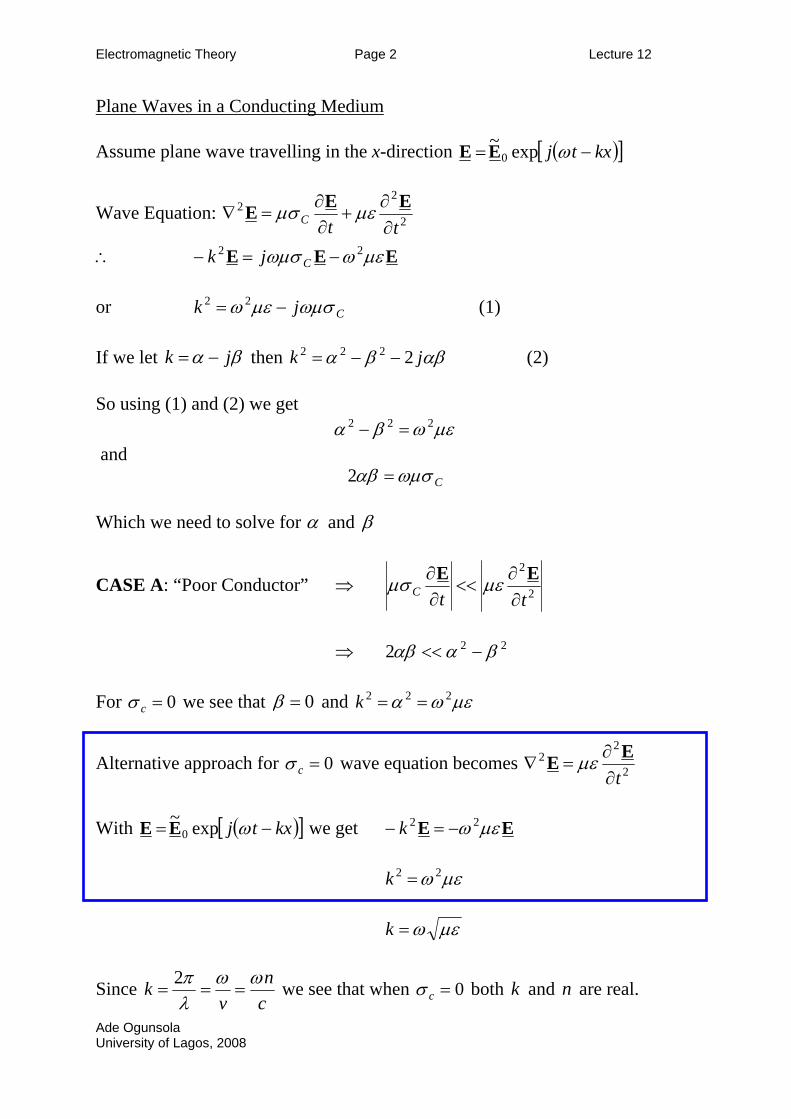
Plane Waves in a Conducting Medium Assume plane wave travelling in the x-direction ( )[ ]kxtj −= ωexp~
0EE
Wave Equation: 2
22
ttC ∂∂
+∂∂
=∇EEE µεµσ
∴ EEE µεωωµσ 22 −=− Cjk or (1) Cjk ωµσµεω −= 22
If we let βα jk −= then (2) αββα jk 2222 −−= So using (1) and (2) we get
µεωβα 222 =− and
Cωµσαβ =2 Which we need to solve for α and β
CASE A: “Poor Conductor” ⇒ 2
2
ttC ∂∂
<<∂∂ EE µεµσ
⇒ 222 βααβ −<<
For 0=cσ we see that 0=β and µεωα 222 ==k
Alternative approach for 0=cσ wave equation becomes 2
22
t∂∂
=∇EE µε
With ( )[ ]kxtj −= ωexp~
0EE we get EE µεω 22 −=− k
µεω 22 =k µεω=k
Since cn
vk ωω
λπ
===2 we see that when 0=cσ both k and are real. n
Ade Ogunsola University of Lagos, 2008
Electromagnetic Theory Page 3 Lecture 12
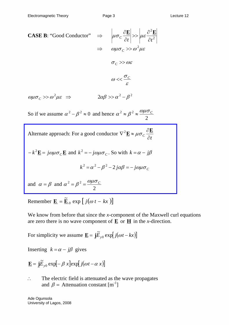
CASE B: “Good Conductor” ⇒ 2
2
ttC ∂∂
>>∂∂ EE µεµσ
⇒ µεωωµσ 2>>C
ωεσ >>C
εσω C<<
µεωωµσ 2>>C ⇒ 222 βααβ −>>
So if we assume and hence 022 ≈− βα2
22 Cωµσβα ≈≈
Alternate approach: For a good conductor tC ∂
∂≈∇
EE µσ2
EE Cjk ωµσ=− 2 and . So with Cjk ωµσ−=2 βα jk −=
Cjjk ωµσαββα −=−−= 2222
and βα = and 2
22 Cωµσβα ==
Remember ( )[ ]kxtj −= ωexp~
0EE We know from before that since the x-component of the Maxwell curl equations are zero there is no wave component of E or H in the x-direction. For simplicity we assume ( )[ ]kxtjEy −= ωexp~
0jE Inserting βα jk −= gives
[ ] ( )[ ]xtjxEy αωβ −−= expexp~0jE
∴ The electric field is attenuated as the wave propagates
and =β Attenuation constant [m-1] Ade Ogunsola University of Lagos, 2008
Electromagnetic Theory Page 4 Lecture 12
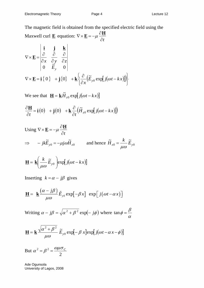
The magnetic field is obtained from the specified electric field using the
Maxwell curl E equation: t∂
∂−=×∇
HE µ
0~0 yEzyx ∂∂
∂∂
∂∂
=×∇
kji
E
( )[ ]( )⎭⎬⎫
⎩⎨⎧
−∂∂
++=×∇ xktjEx y ωexp~00 0kjiE
We see that ( )[ ]xktjH z −= ωexp~
0kH
( ) ( ) ( )[ ]( )xktjHtt z −∂∂
++=∂∂ ωexp~00 0kjiH
Using t∂
∂−=×∇
HE µ
⇒ 00~~
zy HjEjk ωµ−=− and hence 00~~
yz EkHµω
=
( )[ ]xktjEky −⎟⎟⎠
⎞⎜⎜⎝
⎛= ω
µωexp~
0kH
Inserting βα jk −= gives
( ) [ ] ( )0 exp expy
jE x j t
α ββ ω
µω−
= − xα−⎡ ⎤⎣ ⎦H k
Writing ( )φβαβα jj −+=− exp22 where αβφ =tan
[ ] ( )[ ]φαωβµω
βα−−−
+= xtjxEy expexp~
0
22
kH
But 2
22 Cωµσβα ==
Ade Ogunsola
University of Lagos, 2008
Electromagnetic Theory Page 5 Lecture 12
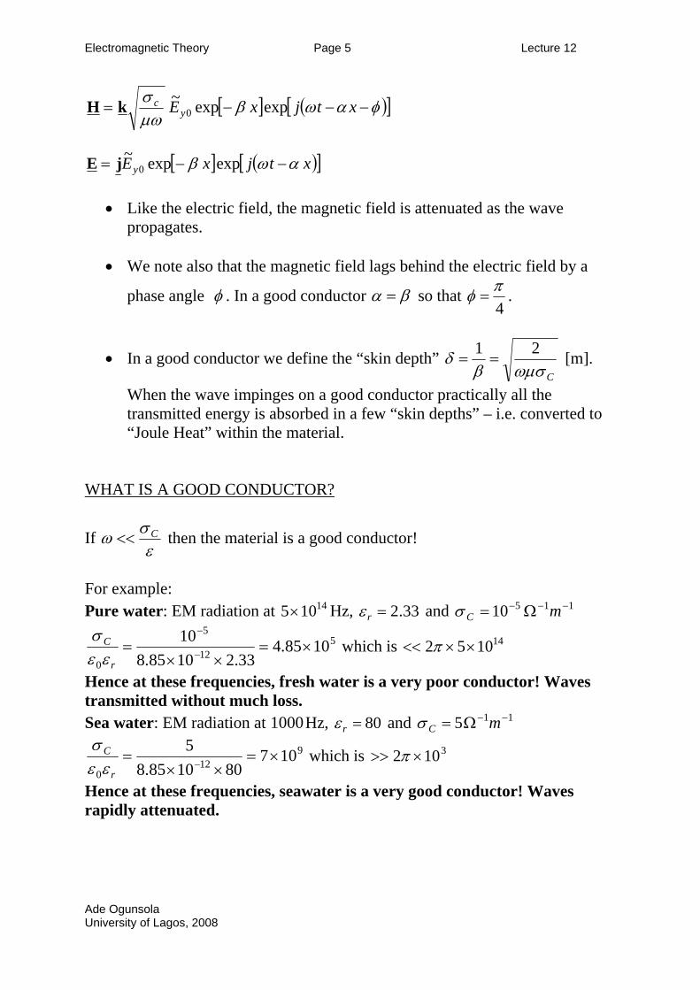
[ ] ( )[ ]φαωβµωσ
−−−= xtjxEyc expexp~
0kH
[ ] ( )[ ]xtjxEy αωβ −−= expexp~
0jE
• Like the electric field, the magnetic field is attenuated as the wave propagates.
• We note also that the magnetic field lags behind the electric field by a
phase angle φ . In a good conductor βα = so that 4πφ = .
• In a good conductor we define the “skin depth” Cωµσβ
δ 21== [m].
When the wave impinges on a good conductor practically all the transmitted energy is absorbed in a few “skin depths” – i.e. converted to “Joule Heat” within the material.
WHAT IS A GOOD CONDUCTOR?
If εσω C<< then the material is a good conductor!
For example: Pure water: EM radiation at 14105× Hz, 33.2=rε and 11510 −−− Ω= mCσ
512
5
01085.4
33.21085.810
×=××
= −
−
r
C
εεσ
which is 141052 ××<< π
Hence at these frequencies, fresh water is a very poor conductor! Waves transmitted without much loss. Sea water: EM radiation at 1000Hz, 80=rε and 115 −−Ω= mCσ
912
0107
801085.85
×=××
= −r
C
εεσ
which is 3102 ×>> π
Hence at these frequencies, seawater is a very good conductor! Waves rapidly attenuated.
Ade Ogunsola University of Lagos, 2008
Electromagnetic Theory Page 1 Lecture 13
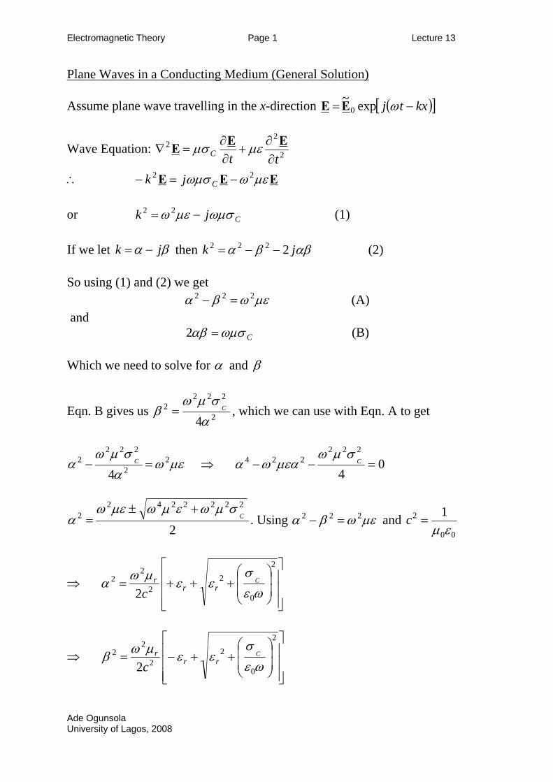
Plane Waves in a Conducting Medium (General Solution) Assume plane wave travelling in the x-direction ( )[ ]kxtj −= ωexp~
0EE
Wave Equation: 2
22
ttC ∂∂
+∂∂
=∇EEE µεµσ
∴ EEE µεωωµσ 22 −=− Cjk or (1) Cjk ωµσµεω −= 22
If we let βα jk −= then (2) αββα jk 2222 −−= So using (1) and (2) we get
µεωβα 222 =− (A) and
Cωµσαβ =2 (B) Which we need to solve for α and β
Eqn. B gives us 2
2222
4ασµω
β C= , which we can use with Eqn. A to get
µεωασµω
α 22
2222
4=− C ⇒ 0
4
222224 =−− C
σµωµεαωα
2
22222422 C
σµωεµωµεωα
+±= . Using and µεωβα 222 =−
00
2 1εµ
=c
⇒ ⎥⎥⎥
⎦
⎤
⎢⎢⎢
⎣
⎡
⎟⎟⎠
⎞⎜⎜⎝
⎛+++=
2
0
22
22
2 ωεσ
εεµωα Crr
r
c
⇒ ⎥⎥⎥
⎦
⎤
⎢⎢⎢
⎣
⎡
⎟⎟⎠
⎞⎜⎜⎝
⎛++−=
2
0
22
22
2 ωεσ
εεµωβ Crr
r
c
Ade Ogunsola University of Lagos, 2008
Electromagnetic Theory Page 2 Lecture 13
Note and 0→C
σ 02 →β µεωα 22 →
Note 1>>εωσ
C 20
22
2 cCr
ε
σωµβα ==
We saw that for [ ] ( )[ ]xtjxEy αωβ −−= expexp~
0jE
we got [ ] ( )[ ]φαωβµω
βα−−−
+= xtjxEy expexp~
0
22
kH
where we have written ( )φβαβα jj −+=− exp22 and αβφ =tan
Refractive Index We should also notice that in a conductor ( )0≠
Cσ the refractive index is
complex
cnk ω
= ⇒ ( ) ( )αββαω
ωµσµεωωω
jcjckcn C 2222
22
2
2
2
222 −−=−==
⎟⎟⎠
⎞⎜⎜⎝
⎛−=
ωεσεµ
0
2 Crr jn
So we see that a complex k means we must have a complex n . So we could write and equate with βα jnnn −= βα jk −= giving
cnαωα = and
cnβω
β =
Now λπω
λπω
αα 22
0===
vn
cn so that we can write
α
λλn
0= and αncv =
The wavelength λ and the velocity in the medium are determined from the free space values by or equivalently
vαn α .
The Range of the wave in the medium is determined by β or equivalently . βn
Ade Ogunsola University of Lagos, 2008
Electromagnetic Theory Page 3 Lecture 13
THE SKIN EFFECT IN GOOD CONDUCTORS: µεωωµσ 2>>C
222 Cωµσβα == and the “skin depth”
Cωµσβδ 21
==
We can now re-write the E field we are using in the previous example as
⎥⎦
⎤⎢⎣
⎡⎟⎠⎞
⎜⎝⎛ −⎥⎦
⎤⎢⎣⎡−=
δω
δxtjxEy expexp~
0jE
Since EJ Cσ=
⎥⎦
⎤⎢⎣
⎡⎟⎠⎞
⎜⎝⎛ −⎥⎦
⎤⎢⎣⎡−=
δω
δxtjxJ y expexp~
0jJ
The E field causes a current to flow in the conductor and the wave energy is dissipated in a few skin depths as Joule Heating and both E and H fields decay to zero. (What happens in a perfect conductor?) Now consider the flow of current down a wire of circular section and radius . a In the D.C. case 0→ω the current density is uniform and 2aJI π= . But at high frequencies practically all the current flow is confined to a thin “sheet” or “skin” at the surface. The maths to show this involves Bessel functions – but if δ>>a then we can find
( )⎥⎦⎤
⎢⎣⎡ −−== = δ
raJJ ar expJ
If δ>>a 95% of the current flows within δ3 of the surface ⇒ hollow conductors are as good as solid ones! Note as 5.0−∝ωδ the higher the frequency the thinner the skin, which implies the higher the resistance since effective area gets smaller as ω increases.
Ade Ogunsola University of Lagos, 2008
Electromagnetic Theory Page 4 Lecture 13
ENERGY TRANSFER BY AN ELECTROMAGNETIC FIELD THE POYNTING VECTOR Start with the Maxwell curl equations:
t∂∂
+=×∇DJH
t∂∂
−=×∇BE
t∂∂
+=×∇ •••DEJEHE
t∂∂
−=×∇ ••BHEH
⎟⎟⎠
⎞⎜⎜⎝
⎛∂∂
+∂∂
−−=×∇−×∇ •••••ttBHDEJEHEEH
For any two vectors YXXYYX ×∇−×∇=×∇ •••
Therefore ⎟⎟⎠
⎞⎜⎜⎝
⎛∂∂
+∂∂
−−=×∇ ••••ttBHDEJEHE
Consider volume bounded by a surface and integrate over the volume v S
∫∫∫ ⎟⎟⎠
⎞⎜⎜⎝
⎛∂∂
+∂∂
−−=×∇ ••••vvv
dvdvdvttBHDEJEHE
HEΠ ×= POYNTING VECTOR [Vm-1][Am-1]=[Wm-2]
Gauss’ Theorem ∫∫ •• =∇
Svddv SΠΠ
∫∫∫ ⎟⎟⎠
⎞⎜⎜⎝
⎛∂∂
+∂∂
−=+ ••••vvS
dvdvdttBHDEJESΠ POYNTING’S
THEOREM For linear and isotropic media: ED ε= and HB µ=
∫∫∫ ⎟⎟⎠
⎞⎜⎜⎝
⎛+
∂∂
−=+ ••v
22
vSdv
2H
2Edvd µε
tJESΠ
Ade Ogunsola University of Lagos, 2008
Electromagnetic Theory Page 5 Lecture 13
Interpretation of Poynting’s Theorem when the volume does not contain a power source.
∫∫∫ ⎟⎟⎠
⎞⎜⎜⎝
⎛+
∂∂
−=+ ••v
22
vSdv
2H
2Edvd µε
tJESΠ
Ade Ogunsola
By conservation of energy this must be the rate at which EM energy is leaving through the surface
v
S⇒ Power flow through S[Js-1=W]
= ∫ ∫=v v2
2
dvJdvJR
Cρ
σ
(using EJ Cσ= ) EM energy is dissipated as Joule Heating within the volume. [Js-1=W]
Sum of the Electric and Magnetic energies in the volume (as derived in statics) =
∫ ⎟⎟⎠
⎞⎜⎜⎝
⎛+
v
22
dv2H
2E µε
∴
∫ ⎟⎟⎠
⎞⎜⎜⎝
⎛+
∂∂
−v
22
dv2H
2E µε
t
= ×−1 (Rate of change of EM energy in the volume). = Rate of decrease of EM energy in the volume. [Js-1=W]
NOTE (1) The EM energy within the volume decreases because some is converted into Joule Heating of the medium and the rest is leaving the volume through its surface. NOTE (2) If ⇒ 0=Cσ . No Joule heating and all of power flowing through the surface
∫∫ ⎟⎟⎠
⎞⎜⎜⎝
⎛+
∂∂
−=•v
22
Sdv
2H
2Ed µε
tSΠ .
NOTE (3) Π= Flux of power through the surface.
University of Lagos, 2008
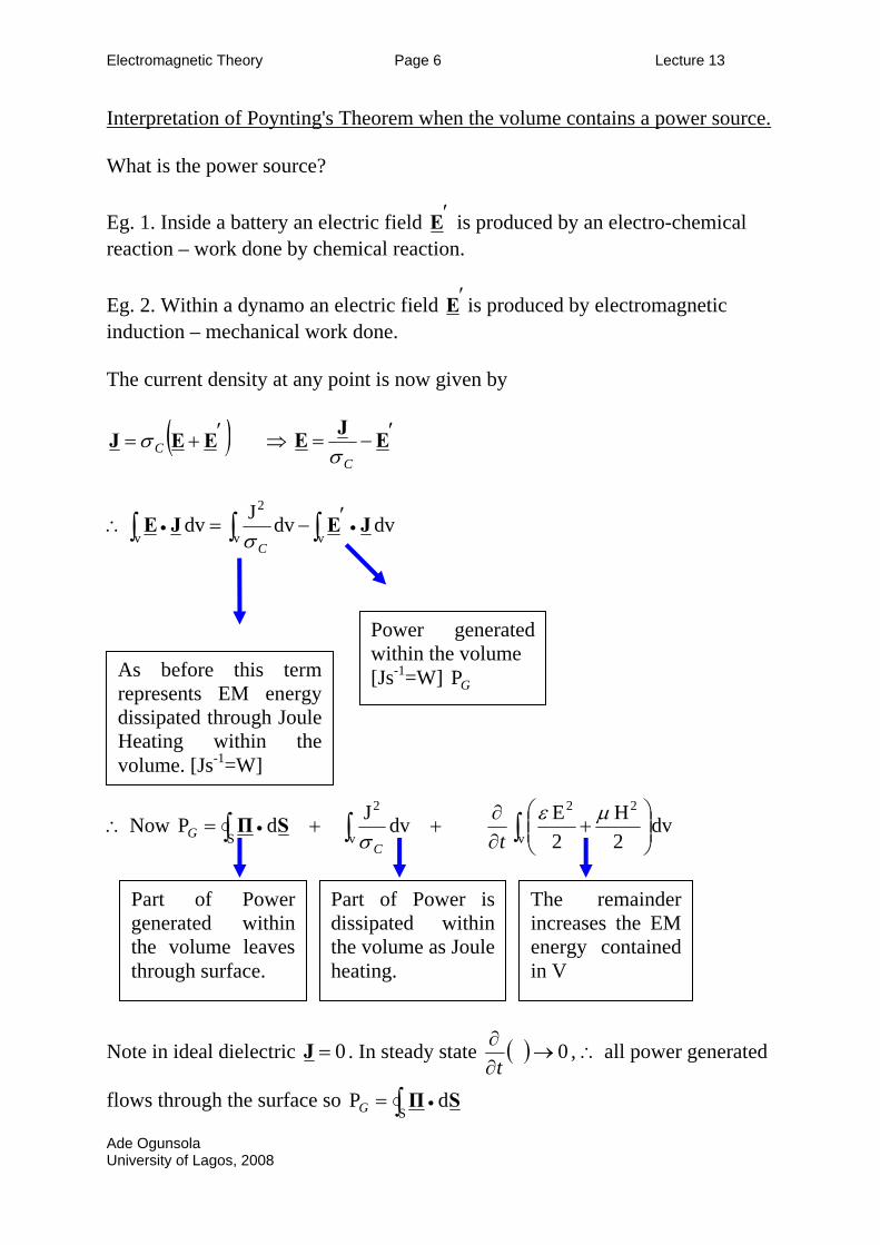
Electromagnetic Theory Page 6 Lecture 13
Interpretation of Poynting's Theorem when the volume contains a power source. What is the power source? Eg. 1. Inside a battery an electric field ′E is produced by an electro-chemical reaction – work done by chemical reaction. Eg. 2. Within a dynamo an electric field ′E is produced by electromagnetic induction – mechanical work done. The current density at any point is now given by
( )′+= EEJ Cσ ⇒ ′−= EJECσ
∴ ∫∫ ∫ ••′−=
vv v
2
dvdvJdv JEJECσ
Power generated
within the volume [Js-1=W] GP
As before this term represents EM energy dissipated through Joule Heating within the volume. [Js-1=W]
∴ Now ∫∫∫ ⎟⎟⎠
⎞⎜⎜⎝
⎛+
∂∂
++= •v
22
v
2
Sdv
2H
2EdvJdP µε
σ tCG SΠ
Part of Power generated within the volume leaves through surface.
Part of Power is dissipated within the volume as Joule heating.
The remainder increases the EM energy contained in V
Note in ideal dielectric 0=J . In steady state ( ) 0→∂∂t
, ∴ all power generated
flows through the surface so ∫ •=S
dP SΠG
Ade Ogunsola University of Lagos, 2008
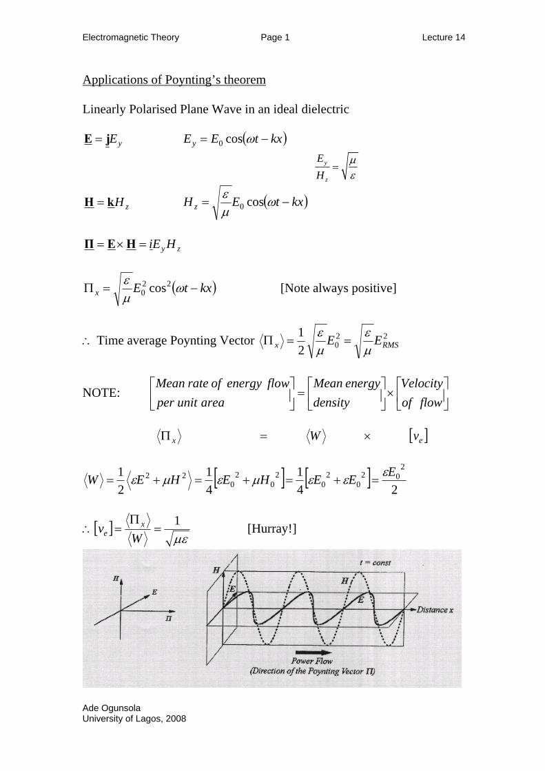
Electromagnetic Theory Page 1 Lecture 14
Ade Ogunsola
Applications of Poynting’s theorem Linearly Polarised Plane Wave in an ideal dielectric
yEjE = ( )kxtEEy −= ωcos0
y
z
EH
µε
=
zHkH = ( )kxtEH z −= ωµε cos0
zy HEi=×= HEΠ
( kxtEx −=Π ωµε 22
0 cos ) [Note always positive]
∴ Time average Poynting Vector 2202
1RMSx EE
µε
µε
==Π
NOTE: ⎥⎦
⎤⎢⎣
⎡×⎥⎦
⎤⎢⎣
⎡=⎥
⎦
⎤⎢⎣
⎡flowof
Velocitydensity
energyMeanareaunitper
flowenergyofrateMean
[ ]ex vW ×=Π
[ ] [ ]24
141
21 2
020
20
20
20
22 EEEHEHEW εεεµεµε =+=+=+=
∴[ ]µε1
=Π
=W
v xe [Hurray!]
University of Lagos, 2008
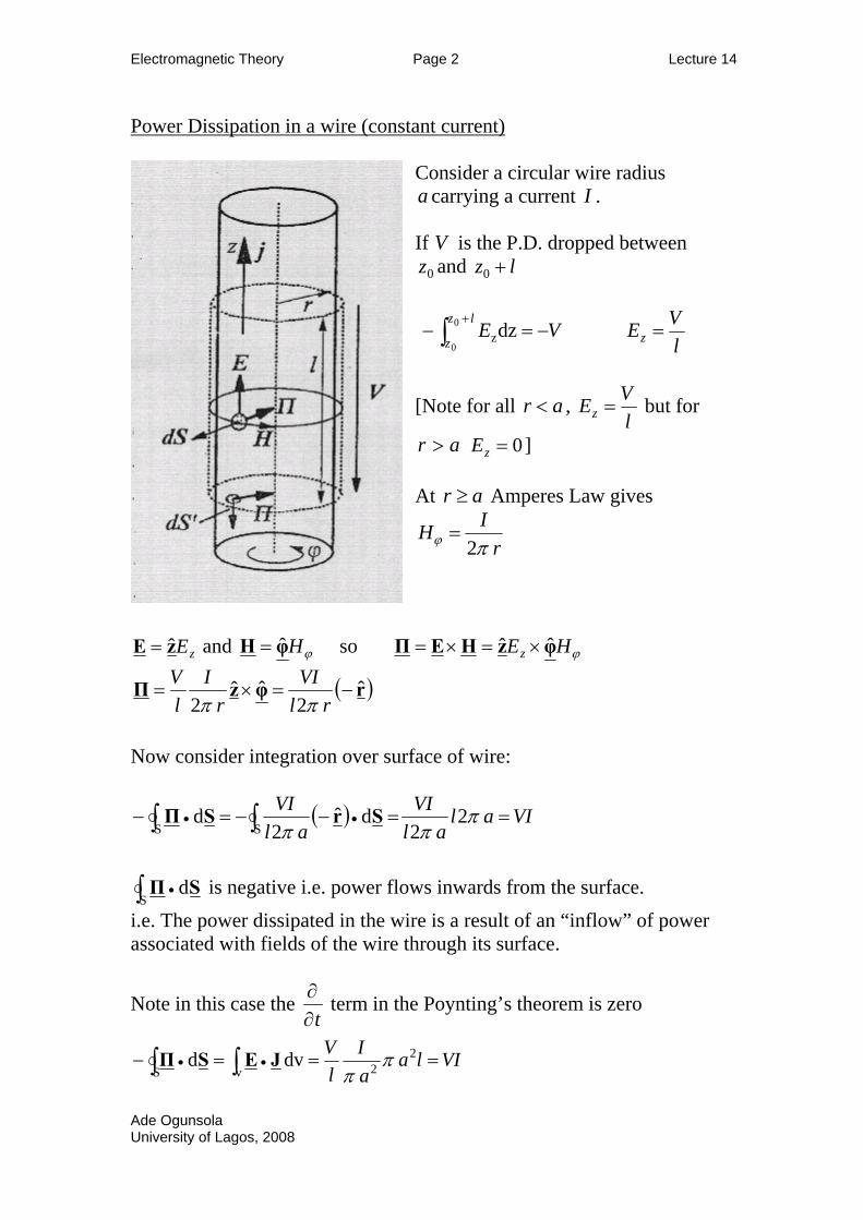
Electromagnetic Theory Page 2 Lecture 14
Ade Ogunsola
Power Dissipation in a wire (constant current) Consider a circular wire radius
carrying a current a I . If V is the P.D. dropped between
and 0z lz +0
∫+
−=−lz
zVE0
0dzz l
VEz =
[Note for all ar < , lVEz = but for
ar > 0=zE ] At ar ≥ Amperes Law gives
rIHπϕ 2
=
zEzE ˆ= and ϕHφH ˆ= so ϕHEz φzHEΠ ˆˆ ×=×=
( )rφzΠ ˆ2
ˆˆ2
−=×=rl
VIr
IlV
ππ
Now consider integration over surface of wire:
( ) VIalal
VIal
VI==−−=− ∫∫ •• π
ππ2
2dˆ
2d
SSSrSΠ
∫ •S
dSΠ is negative i.e. power flows inwards from the surface. i.e. The power dissipated in the wire is a result of an “inflow” of power associated with fields of the wire through its surface.
Note in this case the t∂∂ term in the Poynting’s theorem is zero
VIlaaI
lV
===− ∫∫ ••2
2vSdvd π
πJESΠ
University of Lagos, 2008
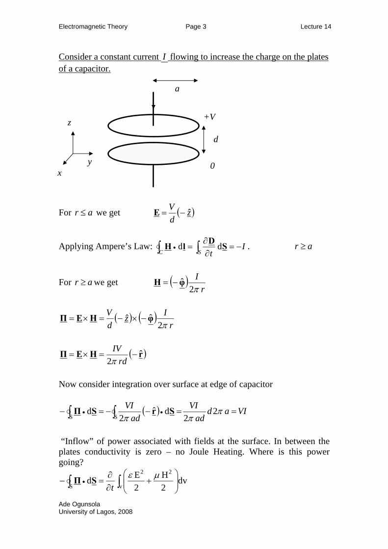
Electromagnetic Theory Page 3 Lecture 14
Ade Ogunsola
Consider a constant current I flowing to increase the charge on the plates of a capacitor. a
+V z
d
y 0 x
For ar ≤ we get ( )zdV ˆ−=E
Applying Ampere’s Law: ItSC
−=∂∂
= ∫∫ • SDlH dd . ar ≥
For ar ≥ we get ( )r
Iπ2
φH −=
( ) ( )r
IzdV
π2ˆˆ φHEΠ −×−=×=
( )rHEΠ ˆ2
−=×=rd
IVπ
Now consider integration over surface at edge of capacitor
( ) VIadad
VIad
VI==−−=− ∫∫ •• π
ππ2
2dˆ
2d
SSSrSΠ
“Inflow” of power associated with fields at the surface. In between the plates conductivity is zero – no Joule Heating. Where is this power going?
∫∫ ⎟⎟⎠
⎞⎜⎜⎝
⎛+
∂∂
=− •v
22
Sdv
2H
2Ed µε
tSΠ
University of Lagos, 2008
Electromagnetic Theory Page 4 Lecture 14
Ade Ogunsola
Electromagnetic Momentum Density : G
BDG ×= [Cm-2Tesla] = [Cm-2NA-1m-1] = [Asm-2NA-1m-1]=[Ns m-3] For linear media
ΠHEHEBDG εµεµµε =×=×=×=
2vΠG =
Radiation Pressure
Consider an EM wave propagating with velocity µε1
=v in a linear
medium. If the wave is incident normally on a totally absorbing surface, then in one second the momentum absorbed per unit area of the surface G.v=
Therefore, v
PrΠ
= [Nm-2]
If the surface is perfectly reflecting v
PrΠ2
=
The Poynting vector and the complex field notation. Suppose that ( )[ ]kxtj −= ωexp~
0EE and ( )[ ]kxtj −= ωexp~
0HH Then ( tj )ω2exp∝×HE - time average over one period is zero!
( ) ( )HEΠ ReRe ×=
University of Lagos, 2008
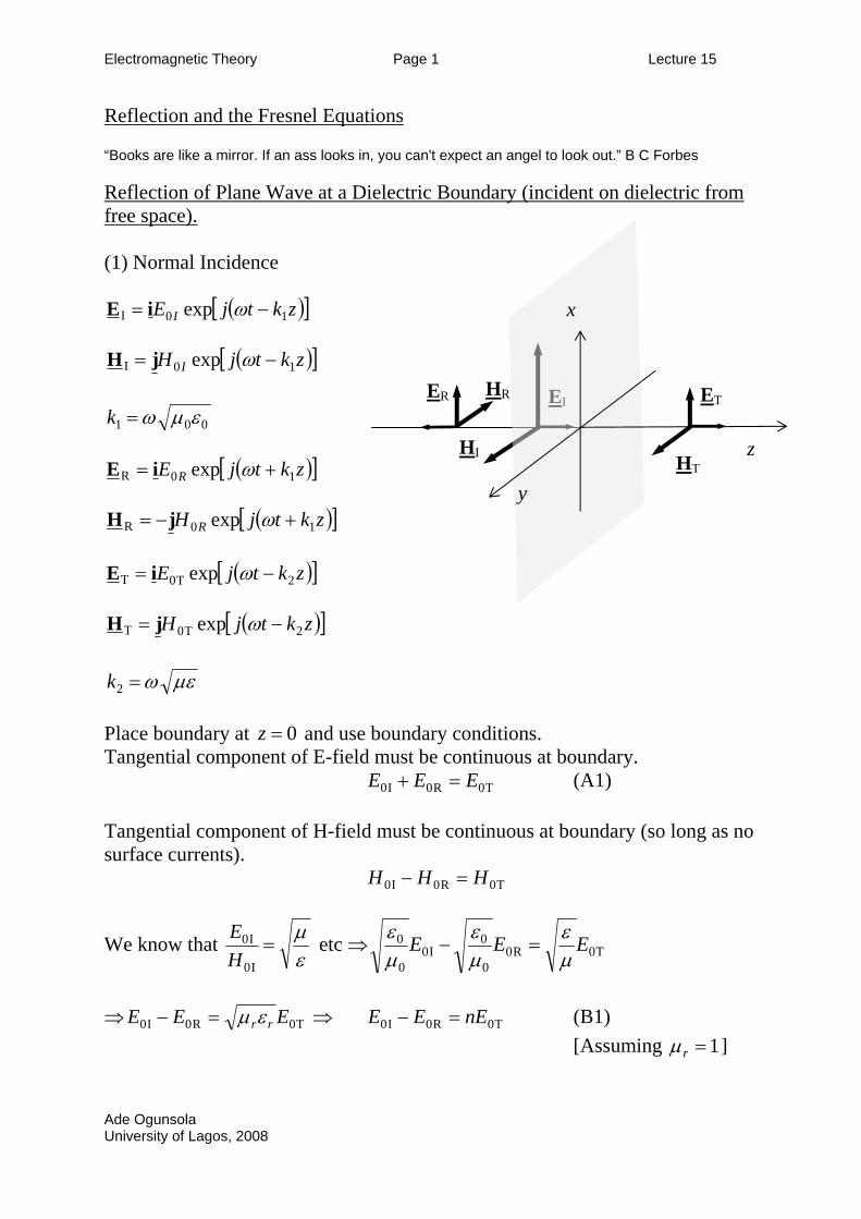
Electromagnetic Theory Page 1 Lecture 15
Reflection and the Fresnel Equations “Books are like a mirror. If an ass looks in, you can't expect an angel to look out.” B C Forbes Reflection of Plane Wave at a Dielectric Boundary (incident on dielectric from free space).
Ade Ogunsola
(1) Normal Incidence
([ zktjE I 10I exp )]−= ωiE
([ zktjH I 10I exp )]−= ωjH
001 εµω=k
([ zktjE R 10R exp )]+= ωiE
( )[ zktjH R 10R exp +−= ]ωjH
([ zktjE 2T0T exp )]−= ωiE
( )[ ]zktjH 2T0T exp −= ωjH
z
ET EI
HT
HR
x
y
ER
HI
µεω=2k
Place boundary at 0=z and use boundary conditions. Tangential component of E-field must be continuous at boundary.
T0R0I0 EEE =+ (A1) Tangential component of H-field must be continuous at boundary (so long as no surface currents).
T0R0I0 HHH =−
We know that εµ
=I0
I0
HE etc ⇒ T0R0
0
0I0
0
0 EEEµε
µε
µε
=−
⇒ T0R0I0 EEE rrεµ=− ⇒ T0R0I0 nEEE =− (B1)
[Assuming 1=rµ ]
University of Lagos, 2008
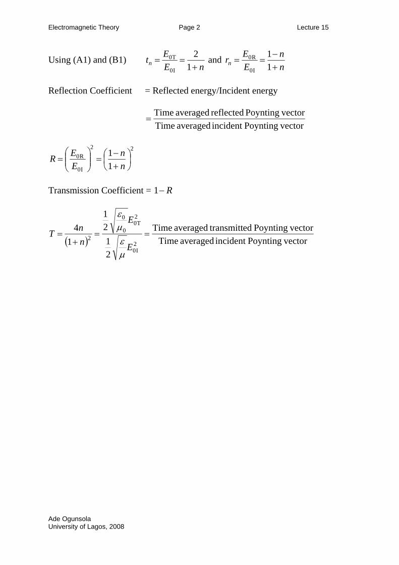
Electromagnetic Theory Page 2 Lecture 15
Using (A1) and (B1) nE
Etn +==
12
I0
T0 and nn
EErn +
−==
11
I0
R0
Reflection Coefficient = Reflected energy/Incident energy
vectorPoyntingincident averaged Time vectorPoynting reflected averaged Time
=
22
I0
R0
11
⎟⎠⎞
⎜⎝⎛+−
=⎟⎟⎠
⎞⎜⎜⎝
⎛=
nn
EER
Transmission Coefficient = R−1
( ) vectorPoyntingincident averaged Time vectorPoynting ed transmittaveraged Time
21
21
14
2I0
2T0
0
0
2 ==+
=E
E
nnT
µεµε
Ade OgunsolaUniversity of Lagos, 2008
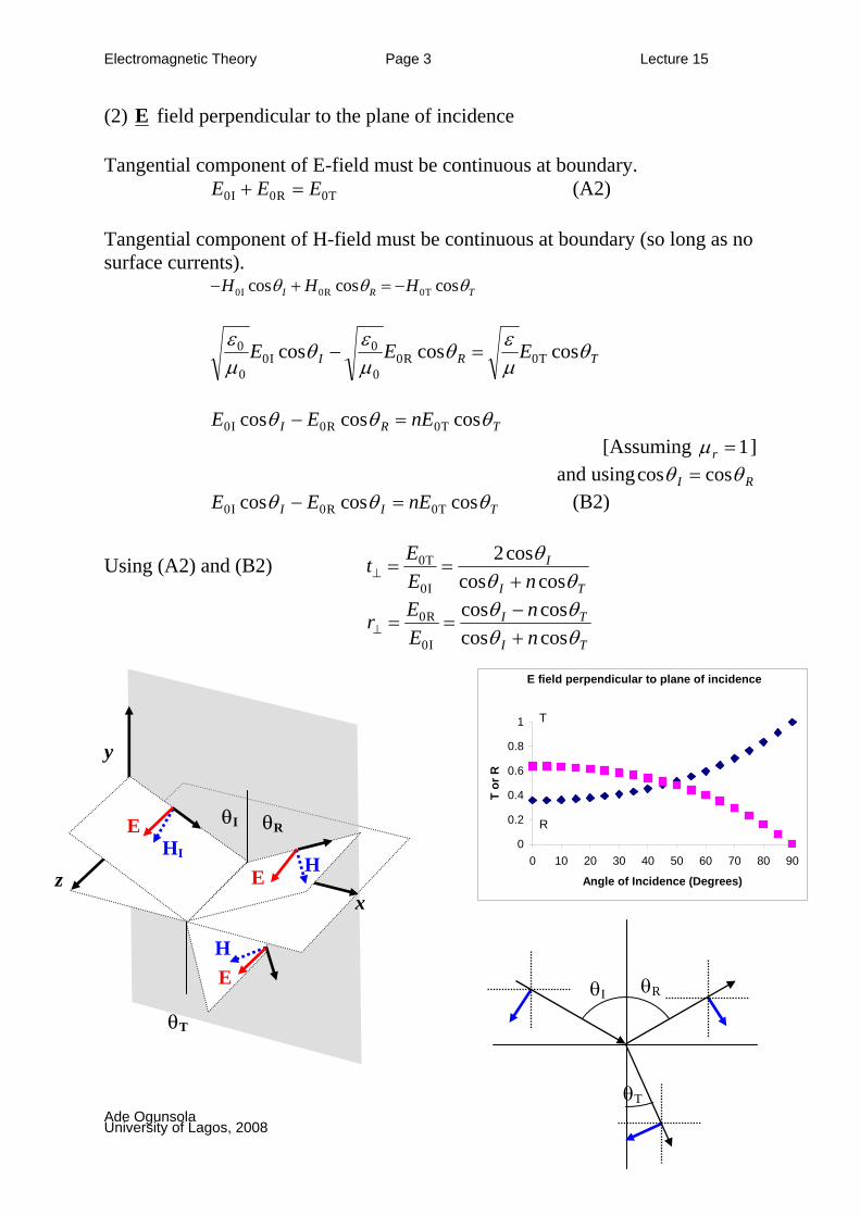
Electromagnetic Theory Page 3 Lecture 15
(2) E field perpendicular to the plane of incidence Tangential component of E-field must be continuous at boundary.
T0R0I0 EEE =+ (A2) Tangential component of H-field must be continuous at boundary (so long as no surface currents).
0I 0R 0Tcos cos cosI R TH H Hθ θ θ− + = −
TRI EEE θµεθ
µεθ
µε coscoscos T0R0
0
0I0
0
0 =−
TRI nEEE θθθ coscoscos T0R0I0 =−
[Assuming 1=rµ ] and using RI θθ coscos =
TII nEEE θθθ coscoscos T0R0I0 =− (B2)
Using (A2) and (B2) TI
I
nEEt
θθθcoscos
cos2
I0
T0
+==⊥
TI
TI
nn
EEr
θθθθ
coscoscoscos
I0
R0
+−
==⊥
θR
θT
y
x
H
EH
θI
E
EHI
E field perpendicular to plane of incidence
0
0.2
0.4
0.6
0.8
1
0 10 20 30 40 50 60 70 80 90
Angle of Incidence (Degrees)
T or
R
T
R
z
θT
θR θI
Ade OgunsolaUniversity of Lagos, 2008
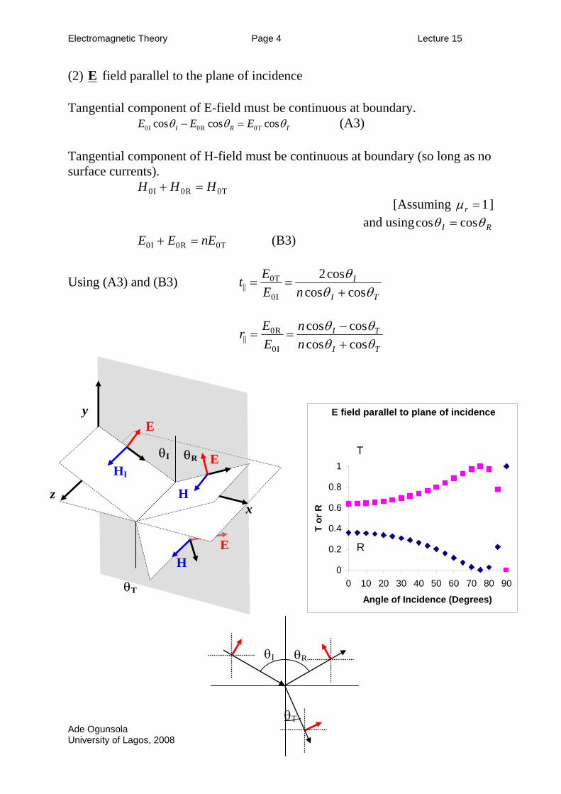
Electromagnetic Theory Page 4 Lecture 15
(2) E field parallel to the plane of incidence Tangential component of E-field must be continuous at boundary.
0I 0R 0Tcos cos cosI RE E E Tθ θ θ− = (A3) Tangential component of H-field must be continuous at boundary (so long as no surface currents).
T0R0I0 HHH =+ [Assuming 1=rµ ]
and using RI θθ coscos = T0R0I0 nEEE =+ (B3)
Using (A3) and (B3) TI
I
nEEt
θθθcoscos
cos2
I0
T0|| +
==
TI
TI
nn
EEr
θθθθ
coscoscoscos
I0
R0|| +
−==
θR
θT
y
x
E
E
E
H
θI
H
HI
E field parallel to plane of incidence
0
0.2
0.4
0.6
0.8
1
0 10 20 30 40 50 60 70 80 90
Angle of Incidence (Degrees)
T or
R
T
R
z
θT
θRθI
Ade Ogunsola University of Lagos, 2008
Electromagnetic Theory Page 5 Lecture 15
Note 1: The formula given above are called the “Fresnel Equations”. Note 2: The formula above can be simplified using Snell’s Law
2211 sinsin θθ nn = , or in our derivations TI n θθ sinsin =
( )( )TI
TIrθθθθ
+−
−=⊥ sinsin ( )
( )TI
TIrθθθθ
+−
=tantan
||
( )TI
ITtθθθθ
+=⊥ sin
cossin2 ( ) ( )TITI
ITtθθθθ
θθ−+
=cossincossin2
||
We see that as 0|| →r2πθθ →+ TI so no light is reflected for this polarisation.
Note also that changes sign at ||r2πθθ =+ TI so there is a phase shift of π in
the reflected parallel components of the E- (and H-) fields when sweeping the incident angle Iθ through the polarisation angle Pθ ( Pθ is the value of Iθ for
which 2πθθ =+ TI ). However, is always negative so no phase change in the
reflected perpendicular components of the E- (and H-) fields. ⊥r
Note 3: Be careful using the Fresnel Equations, must get the polarisation correct! Easy to get confused! Note 4: Can calculate the reflected and transmitted intensities using the Fresnel Equations. Note 5: Could derive the Fresnel Equations for transmission a boundary where
and investigate total internal reflection…but not here! See for example Optics (Second Edition) by Hecht.
TI nn >
Ade Ogunsola University of Lagos, 2008
Electromagnetic Theory Page 6 Lecture 15
Reflection at a conducting boundary. Consider the case where plane wave travelling in free space strikes at normal incidence a conducting boundary
([ zktjE I 10I exp )]−= ωiE 001 εµω=k ([ zktjH I 10I exp )]−= ωjH
([ zktjE R 10R exp )]+= ωiE
( )[ ]zktjH R 10R exp +−= ωjH
[ ] ([ ztjzE TT )]αωβ −−= expexp0iE βα jk −=2
[ ] ( )[ ]zktjzH TT −−= ωβ expexp0jH
( ) [ ] ( )[ ]zktjzEjTT −−
−= ωβ
µωβα expexp0jH (See lecture 12)
Boundary at 0=z . Tangential component of E-field must be continuous at boundary.
T0R0I0 EEE =+ (A4) Tangential component of H-field must be continuous at boundary (so long as no surface current unit length flowing on the boundary, i.e. we have a good conductor not a perfect conductor).
T0R0I0 HHH =−
( )TEjEE 0R0
0
0I0
0
0
µωβα
µε
µε −
=−
For a good conductor 2
Cωµσβα ==
( ) Tr
C EjEE 00
R0I0 21
εωµσ
−=− (B4)
Ade Ogunsola University of Lagos, 2008
Electromagnetic Theory Page 7 Lecture 15
Using (A4) and (B4)
( )
( )0
0
I0
R0
211
211
εωµσ
εωµσ
r
C
r
C
n
j
j
EEr
−+
−−==
C
rn E
ERσ
εωµ 02
I0
R0 221−≈⎟⎟⎠
⎞⎜⎜⎝
⎛=
For copper at infrared frequencies (around 1014 Hz) 01.02 0 ≈C
r
σεωµ , so about
98% of infrared radiation is reflected, the remainder is absorbed in the metal due to Joule Heating.
At lower frequencies (e.g. radio waves) 60 102 −≈C
r
σεωµ almost all radiation is
reflected. At higher frequencies (>1015 Hz), simple theory does not work, we need to take account of the atomic transitions that take place and give rise to the colour of the metal.
Ade Ogunsola University of Lagos, 2008

![[X-&)( · 9l)*rV)X-"["Z*.\[] ^ ]_X-!+&!+i lL\ZX-" ]_XY&U^ K\Z^+(#!#aL,-X XY"%^+f)f)\[! #* V \[* (otO!+][]_XY* +!#lL& 'X-,-,-^+"Z*.&)!#\ tO^+&U^+(#XY!+]_XY" l)\[X-"[]Z!](https://img.pdfslide.us/doc/110x75/5e7162f7c481ba77d90de1c1/x-9lrvx-z-x-i-llzx-xyu.jpg)