Embed Size (px)
Citation preview
1
Electromagnetic Ring Launcher
A Major Qualifying Project
Submitted to the Faculty of the
WORCESTER POLYTECHNIC INSTITUTE
In partial fulfillment of the requirements for the degree of
Bachelor of Science
by
Ali Algarni
Frank Gleason
Ashwin Mohanakumaran
Submitted: April 30, 2014
Approved by:
Professor Alexander Emanuel, Project Advisor

2
Table of Contents
Abstract ......................................................................................................................................................... 3
Acknowledgements ....................................................................................................................................... 4
Authorship .................................................................................................................................................... 4
Introduction: .................................................................................................................................................. 5
Overview: ...................................................................................................................................................... 7
Chapter 1: System Design and Component Specifications ........................................................................... 9
Power Supply .......................................................................................................................................... 10
Diode and Resistor .................................................................................................................................. 10
Capacitor ................................................................................................................................................. 10
Switch ..................................................................................................................................................... 11
Acrylic Tube ........................................................................................................................................... 11
Magnetic Coil.......................................................................................................................................... 12
Aluminum Rings ..................................................................................................................................... 15
Chapter 2: The Self – Triggering Circuit .................................................................................................... 23
SCR ......................................................................................................................................................... 24
................................................................................................................................................................ 25
Transmitter and Receiver Circuit ............................................................................................................ 25
Chapter 3: Optimum Parameters ................................................................................................................. 29
Finding the Ideal Height for Launch: ...................................................................................................... 29
Speed testing circuit ................................................................................................................................ 39
Chapter 4 – Project Simulation ................................................................................................................... 42
PSpice Simulation ................................................................................................................................... 42
Optimizing the System – Force, Velocity, and Height ........................................................................... 49
Experimenting With the Source Voltage ................................................................................................ 54
Implementing a Second Station .............................................................................................................. 57
Conclusion: ................................................................................................................................................. 61
Appendix A ................................................................................................................................................. 62
Appendix B - Calculations of Lyle’s Method ............................................................................................. 63
References .................................................................................................................................................. 64
3
Abstract
Electromagnetics have a wide variety of applications in today’s world. Developments
such as the railgun and the Hyperloop demonstrate the use of electromagnetism in projectile
launchers. The objective of this MQP is to understand the variables and possible issues
associated with an electromagnetic launcher through the construction of a ring launcher similar
to a coilgun. This project also seeks to measure the optimum parameters to achieve the highest
efficiency for a launch and design a self-triggering circuit to allow the launcher to perform
without human interaction.
4
Acknowledgements
We would like to extend our sincerest gratitude and thanks to Professor Alexander
Emanuel whose vision and support guided us throughout this project. His experience and
intellect were a major part of the driving force that led to this project’s success.
We would also like to thank Robert Boisse for his support in the acquisition of parts for
the project and his willingness to help through the Electrical and Computer Engineering shop in
Atwater Kent.
Authorship
Chapter 1 Ali Algarni
Chapter 2 Ali Algarni
Chapter 3 Ashwin Mohanakumaran
Chapter 4 Frank Gleason
5
Introduction:
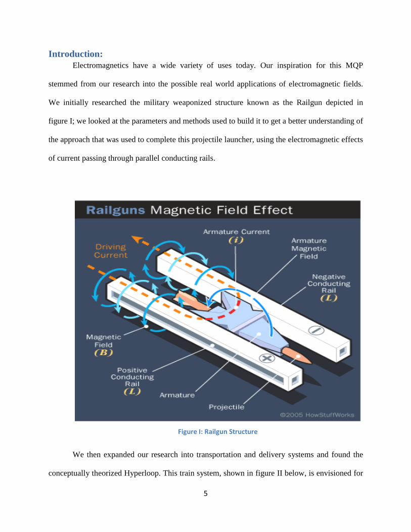
Electromagnetics have a wide variety of uses today. Our inspiration for this MQP
stemmed from our research into the possible real world applications of electromagnetic fields.
We initially researched the military weaponized structure known as the Railgun depicted in
figure I; we looked at the parameters and methods used to build it to get a better understanding of
the approach that was used to complete this projectile launcher, using the electromagnetic effects
of current passing through parallel conducting rails.
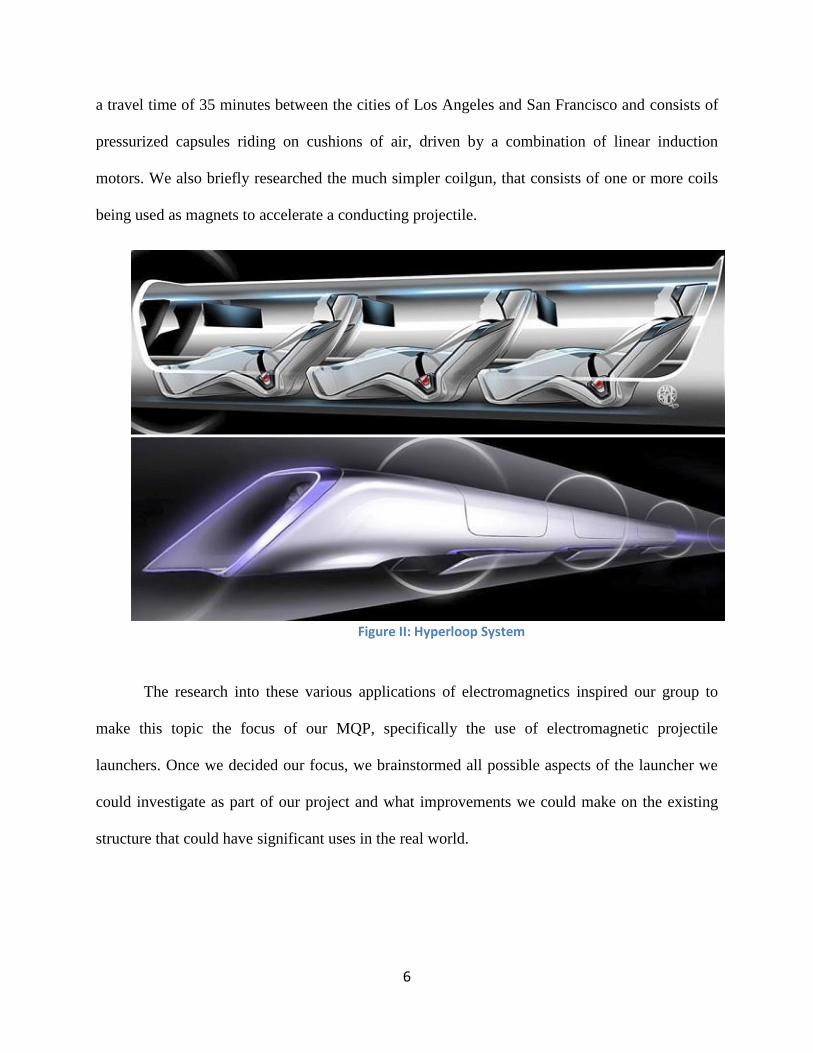
We then expanded our research into transportation and delivery systems and found the
conceptually theorized Hyperloop. This train system, shown in figure II below, is envisioned for
Figure I: Railgun Structure
6
a travel time of 35 minutes between the cities of Los Angeles and San Francisco and consists of
pressurized capsules riding on cushions of air, driven by a combination of linear induction
motors. We also briefly researched the much simpler coilgun, that consists of one or more coils
being used as magnets to accelerate a conducting projectile.
The research into these various applications of electromagnetics inspired our group to
make this topic the focus of our MQP, specifically the use of electromagnetic projectile
launchers. Once we decided our focus, we brainstormed all possible aspects of the launcher we
could investigate as part of our project and what improvements we could make on the existing
structure that could have significant uses in the real world.
Figure II: Hyperloop System

7
Overview:
Once the focus of our MQP was decided, the major tasks and accomplishments to be
achieved within the one year span had to be outlined. Since our goal was to construct a simpler
version of a projectile launcher, it was decided to use small metallic rings as the projectile. This
would allow safe conduction of experiments and easier manipulation of the projectile to
understand the significance of its dimensions to the success of the overall launch.
When constructing any major appliance without extensive prior knowledge, it is
important to understand its mechanisms thoroughly. This became the first objective of this MQP;
to understand the various parameters involved with the electromagnetic ring launcher and how
each of these variables contributes to a launch. These include each of the components of the
actual launcher, their interactions with each other and the electromagnetic characteristics of the
apparatus.
Once the parameters and the launcher’s structure were understood, the objective became
to expand on the existing model with additions that can prove beneficial in existing applications.
Initially the idea was to expand the launcher by adding a secondary launch mechanism; however,
due to budget restrictions and the lack of availability of certain parts, this became a very difficult
task to achieve. Another useful addition envisioned for the electromagnetic ring launcher was the
removal of any human interaction with the launcher, in regards to the trigger and having the
device self-trigger. In larger applications, this can significantly remove any safety hazards
associated with the launcher and in the case of weaponized structures, ensure minimum risk. This
became one of the major objectives for the project.

8
Once the components of the launcher, their interactions with each other and the numerous
physical characteristics involved in this project were understood, it was important to learn the
effects of changes in physical structures and placements on a specific launch. This was partly
achieved through the use of a speed testing circuit, which was used in conjunction with the self-
triggering mechanism to observe the change in speed of a launch under different conditions.
Studying these effects involved using theoretical knowledge and calculations made of the system
and testing them practically. This not only validated the theory behind the launcher but also
helped us acquire the optimum parameters for a launch. This ensures maximum efficiency for the
device and is essential knowledge when applying larger projectile structures.
The final objective of this project was to use the theory and knowledge at hand and
simulate the launcher using PSpice software. This not only helped better understand the
interactions involved in the launcher but also allowed for testing of conditions that would be
difficult to achieve experimentally. Although a secondary launch system was not constructed
physically, simulations in PSpice also allowed us to see the effects such an addition would have
on the existing structure and the optimum parameters for such an installation to occur.
9
Chapter 1: System Design and Component Specifications
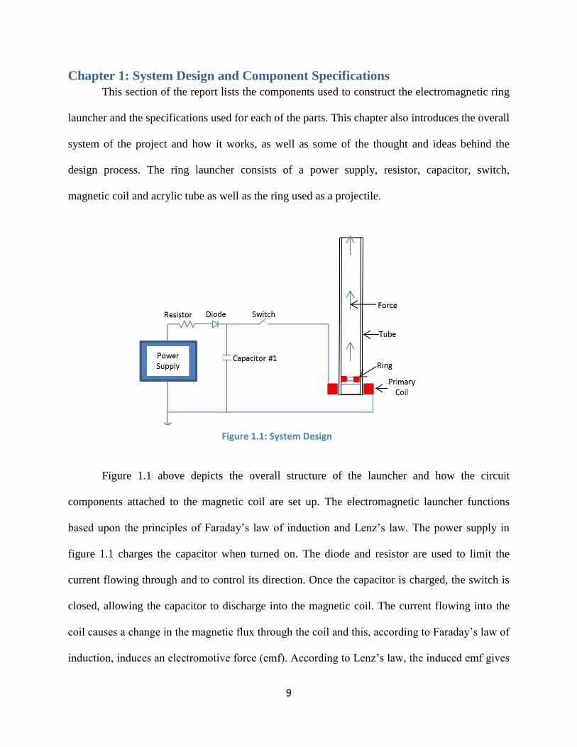
This section of the report lists the components used to construct the electromagnetic ring
launcher and the specifications used for each of the parts. This chapter also introduces the overall
system of the project and how it works, as well as some of the thought and ideas behind the
design process. The ring launcher consists of a power supply, resistor, capacitor, switch,
magnetic coil and acrylic tube as well as the ring used as a projectile.
Figure 1.1 above depicts the overall structure of the launcher and how the circuit
components attached to the magnetic coil are set up. The electromagnetic launcher functions
based upon the principles of Faraday’s law of induction and Lenz’s law. The power supply in
figure 1.1 charges the capacitor when turned on. The diode and resistor are used to limit the
current flowing through and to control its direction. Once the capacitor is charged, the switch is
closed, allowing the capacitor to discharge into the magnetic coil. The current flowing into the
coil causes a change in the magnetic flux through the coil and this, according to Faraday’s law of
induction, induces an electromotive force (emf). According to Lenz’s law, the induced emf gives
Figure 1.1: System Design

10
rise to a current whose magnetic field opposes the original change in magnetic flux. As such, the
current through the coil will induce a current in the ring in the opposite direction. These two
currents will repel each other and cause the ring to launch upwards through the tube.
Power Supply
The power supply used for this launcher had a range of 350 – 500V. This variation in
voltage was used in various tests explained later in the report. For the standard launch used to
demonstrate the functionality of the launcher, an output of 400V from the power supply was
used.
Diode and Resistor
The diode in figure 1.1 is used to control the direction of the current flow from the power
supply and ensure its moves flows to the capacitor. A resistor of 4.7 kΩ is used to limit the
current going into the capacitors.
Capacitor
A combination of capacitors was used in this circuit to achieve the desired launch. The
configuration of the capacitors produced 300 µF and these capacitors were specifically chosen to
have low internal resistances and be capable of charging and discharging in relatively short
periods of time, so as to increase the efficiency of the launcher.
11
Switch
The purpose of the switch in figure 1.1 is to trigger the launch of the ring through the
tube. The switch is left open while the capacitor is charging and when required, it is closed,
allowing the current to pass through to the coil and launch the ring. The switch’s implementation
in this circuit had to be modified as part of the project to have the launcher self-trigger and this is
discussed in chapter 2 of the report.
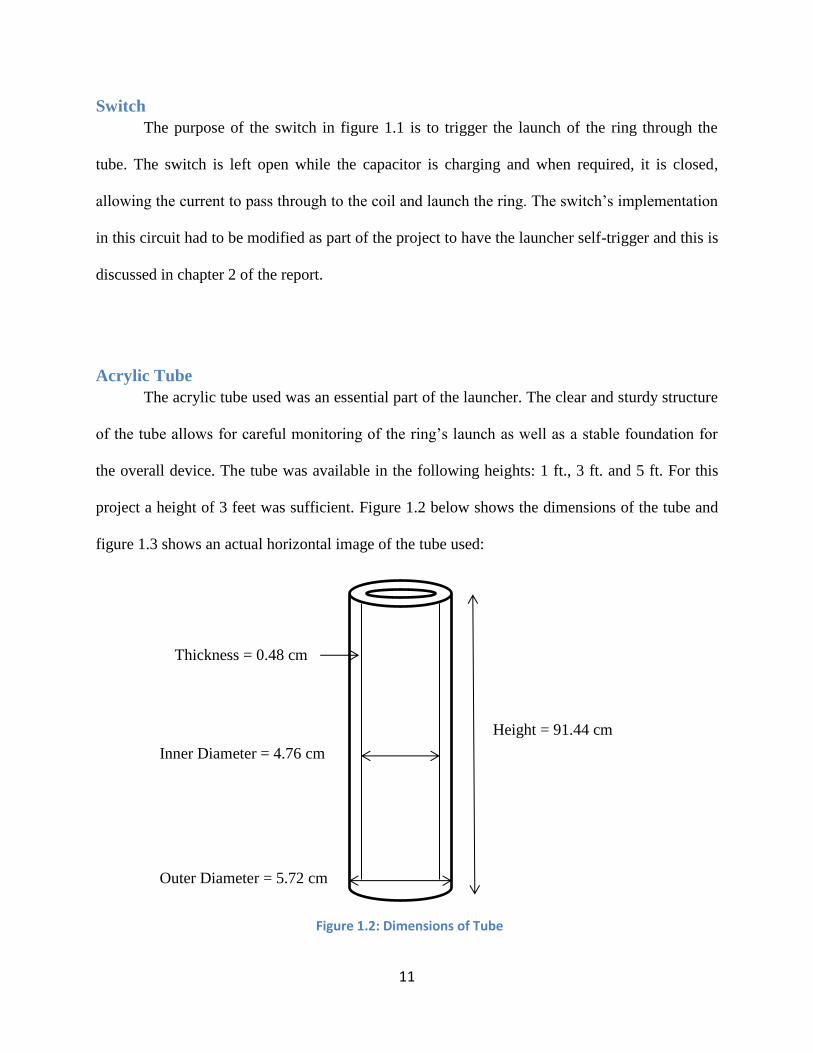
Acrylic Tube
The acrylic tube used was an essential part of the launcher. The clear and sturdy structure
of the tube allows for careful monitoring of the ring’s launch as well as a stable foundation for
the overall device. The tube was available in the following heights: 1 ft., 3 ft. and 5 ft. For this
project a height of 3 feet was sufficient. Figure 1.2 below shows the dimensions of the tube and
figure 1.3 shows an actual horizontal image of the tube used:
Height = 91.44 cm
Inner Diameter = 4.76 cm
Thickness = 0.48 cm
Outer Diameter = 5.72 cm
Figure 1.2: Dimensions of Tube
12
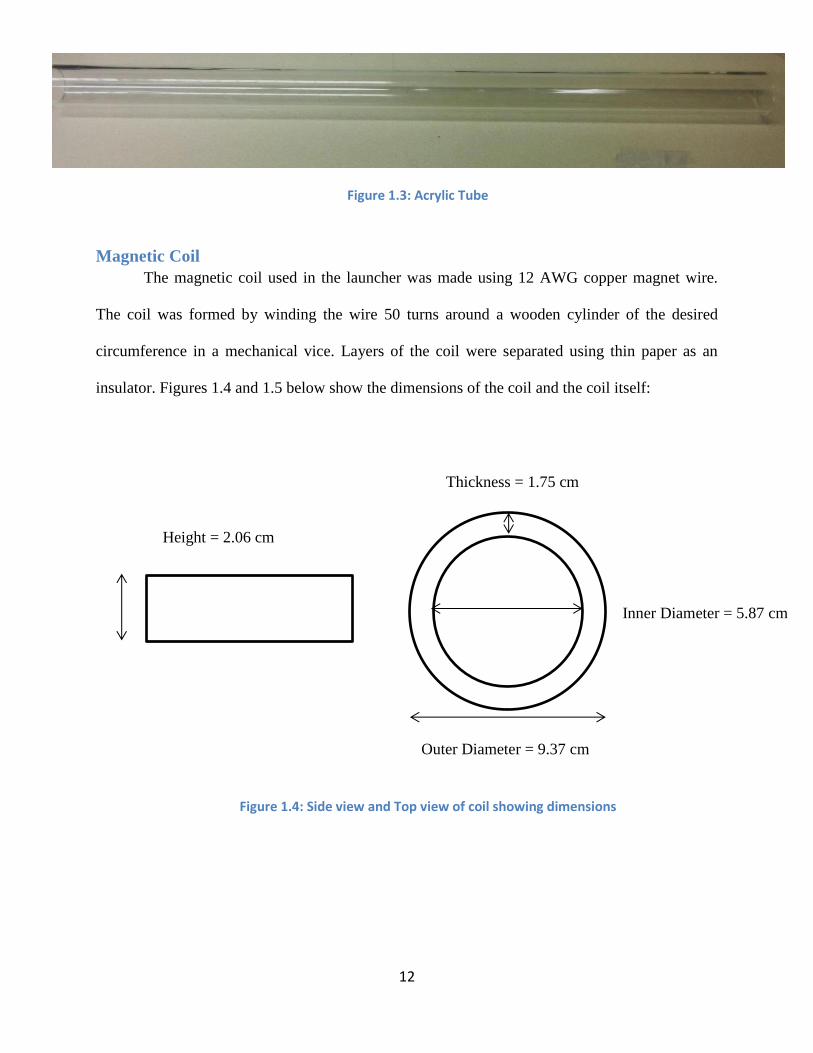
Magnetic Coil
The magnetic coil used in the launcher was made using 12 AWG copper magnet wire.
The coil was formed by winding the wire 50 turns around a wooden cylinder of the desired
circumference in a mechanical vice. Layers of the coil were separated using thin paper as an
insulator. Figures 1.4 and 1.5 below show the dimensions of the coil and the coil itself:
Figure 1.3: Acrylic Tube
Height = 2.06 cm
Thickness = 1.75 cm
Inner Diameter = 5.87 cm
Outer Diameter = 9.37 cm
Figure 1.4: Side view and Top view of coil showing dimensions
13
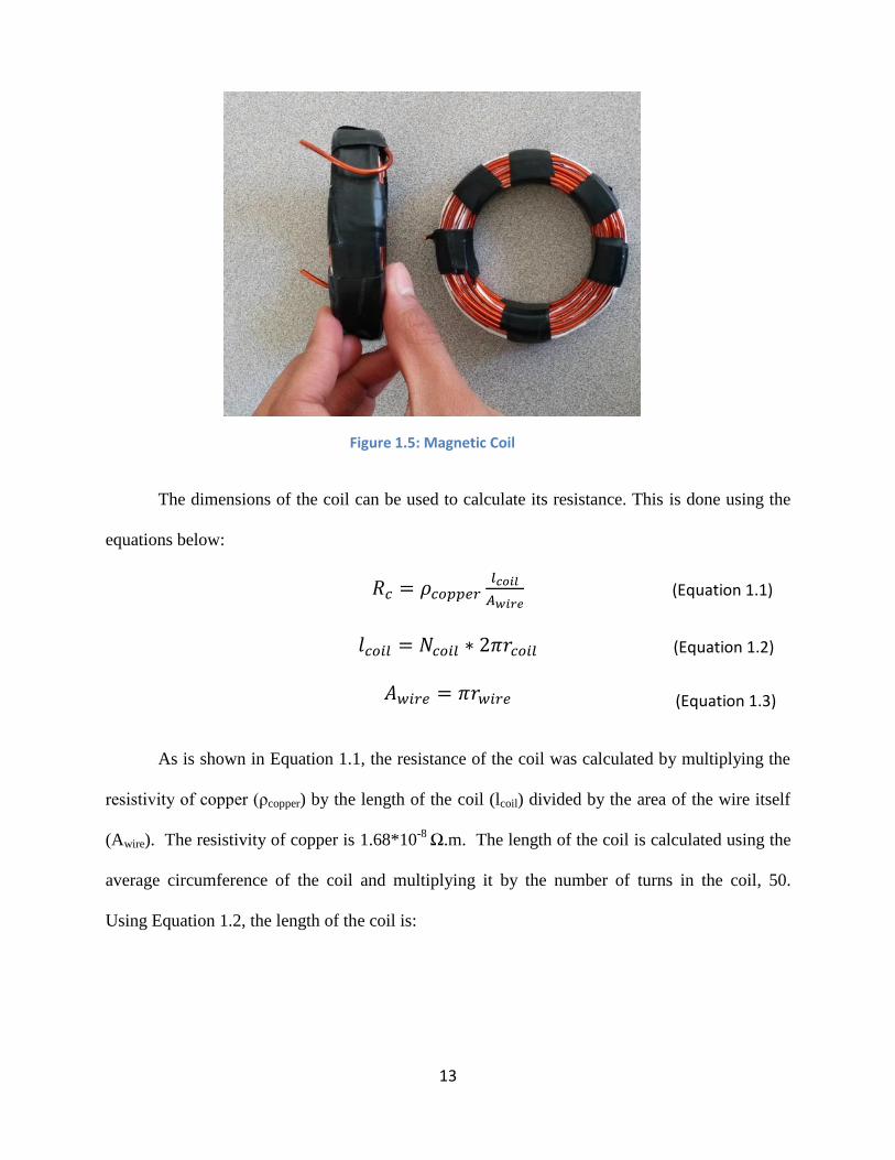
The dimensions of the coil can be used to calculate its resistance. This is done using the
equations below:
As is shown in Equation 1.1, the resistance of the coil was calculated by multiplying the
resistivity of copper (ρcopper) by the length of the coil (lcoil) divided by the area of the wire itself
(Awire). The resistivity of copper is 1.68*10-8
Ω.m. The length of the coil is calculated using the
average circumference of the coil and multiplying it by the number of turns in the coil, 50.
Using Equation 1.2, the length of the coil is:
Figure 1.5: Magnetic Coil
(Equation 1.1)
(Equation 1.2)
(Equation 1.3)
14
Using Equation 1.3, the area of the wire itself is calculated as:
Substituting these values into Equation 1.1, the resistance of the coil is:
( )
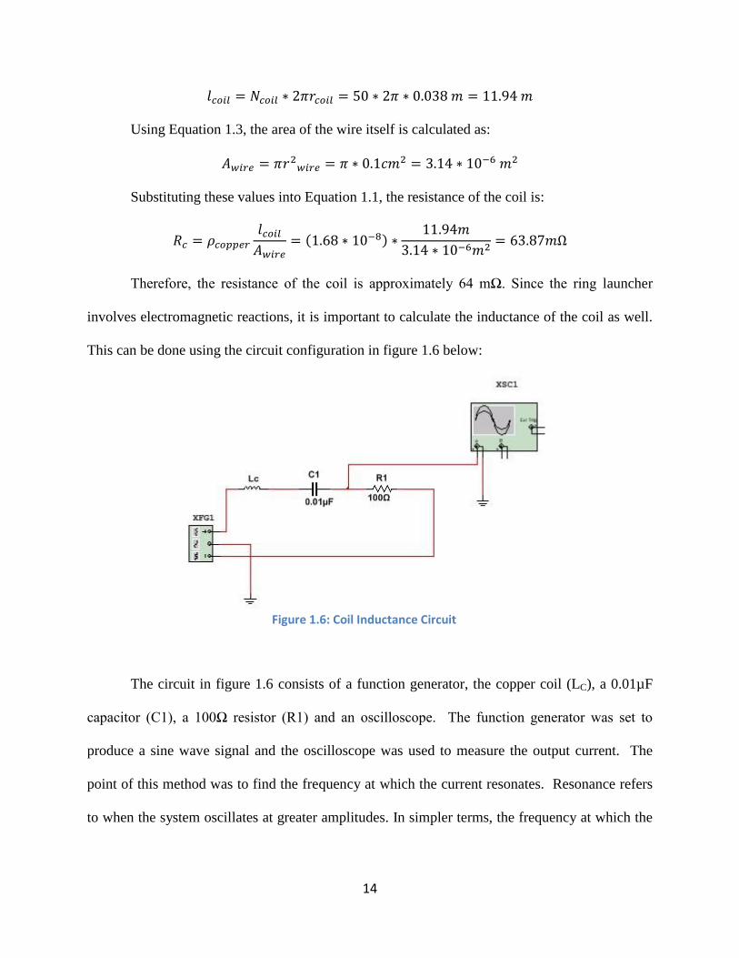
Therefore, the resistance of the coil is approximately 64 mΩ. Since the ring launcher
involves electromagnetic reactions, it is important to calculate the inductance of the coil as well.
This can be done using the circuit configuration in figure 1.6 below:
The circuit in figure 1.6 consists of a function generator, the copper coil (LC), a 0.01µF
capacitor (C1), a 100Ω resistor (R1) and an oscilloscope. The function generator was set to
produce a sine wave signal and the oscilloscope was used to measure the output current. The
point of this method was to find the frequency at which the current resonates. Resonance refers
to when the system oscillates at greater amplitudes. In simpler terms, the frequency at which the
Figure 1.6: Coil Inductance Circuit
15
Equation 1.4
Equation 1.5
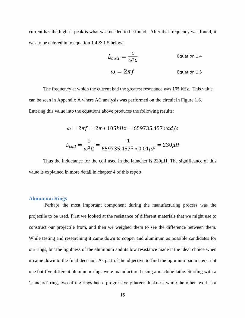
current has the highest peak is what was needed to be found. After that frequency was found, it
was to be entered in to equation 1.4 & 1.5 below:
The frequency at which the current had the greatest resonance was 105 kHz. This value
can be seen in Appendix A where AC analysis was performed on the circuit in Figure 1.6.
Entering this value into the equations above produces the following results:
Thus the inductance for the coil used in the launcher is 230µH. The significance of this
value is explained in more detail in chapter 4 of this report.
Aluminum Rings
Perhaps the most important component during the manufacturing process was the
projectile to be used. First we looked at the resistance of different materials that we might use to
construct our projectile from, and then we weighed them to see the difference between them.
While testing and researching it came down to copper and aluminum as possible candidates for
our rings, but the lightness of the aluminum and its low resistance made it the ideal choice when
it came down to the final decision. As part of the objective to find the optimum parameters, not
one but five different aluminum rings were manufactured using a machine lathe. Starting with a
‘standard’ ring, two of the rings had a progressively larger thickness while the other two has a
16
progressively larger height. The testing of these rings is covered in chapter 3. The rings were
numbered 1 through 5, with the ‘standard’ ring being 1, the thicker rings being 2 and 3 and the
taller rings being 4 and 5. The only dimension kept the same between the rings was the outer
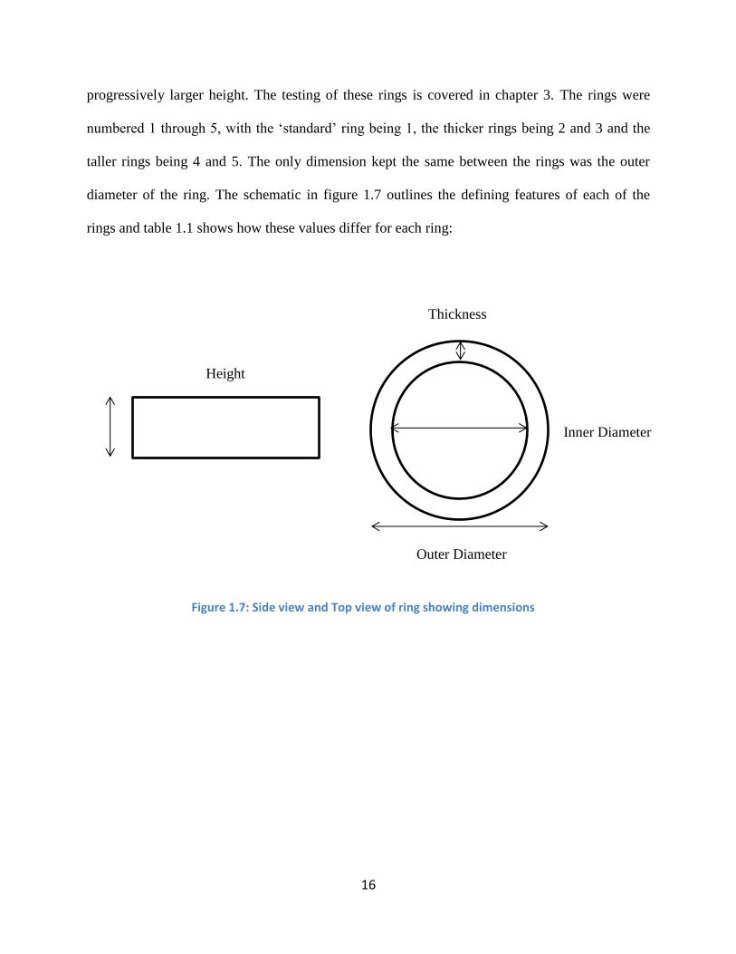
diameter of the ring. The schematic in figure 1.7 outlines the defining features of each of the
rings and table 1.1 shows how these values differ for each ring:
Height
Thickness
Inner Diameter
Outer Diameter
Figure 1.7: Side view and Top view of ring showing dimensions
17
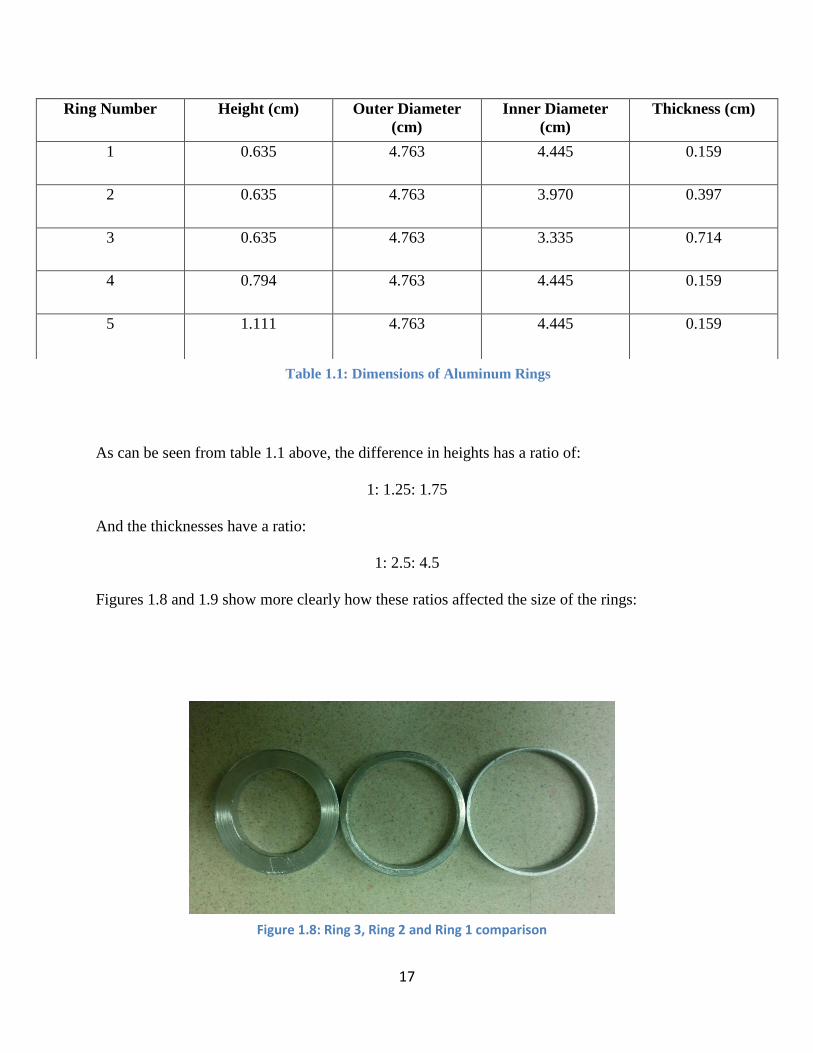
As can be seen from table 1.1 above, the difference in heights has a ratio of:
1: 1.25: 1.75
And the thicknesses have a ratio:
1: 2.5: 4.5
Figures 1.8 and 1.9 show more clearly how these ratios affected the size of the rings:
Ring Number Height (cm) Outer Diameter
(cm)
Inner Diameter
(cm)
Thickness (cm)
1 0.635 4.763 4.445 0.159
2 0.635 4.763 3.970 0.397
3 0.635 4.763 3.335 0.714
4 0.794 4.763 4.445 0.159
5 1.111 4.763 4.445 0.159
Table 1.1: Dimensions of Aluminum Rings
Figure 1.8: Ring 3, Ring 2 and Ring 1 comparison
18
(Equation 1.6)
(Equation 1.7)
:
.
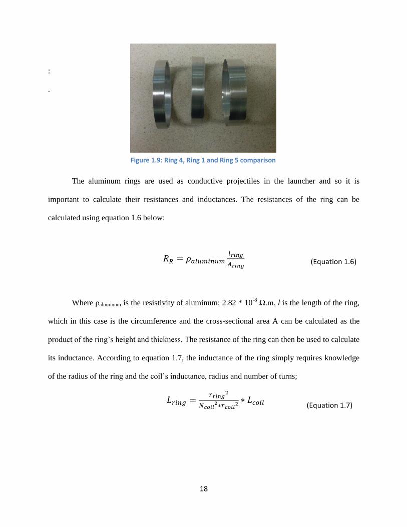
The aluminum rings are used as conductive projectiles in the launcher and so it is
important to calculate their resistances and inductances. The resistances of the ring can be
calculated using equation 1.6 below:
Where ρaluminum is the resistivity of aluminum; 2.82 * 10-8
Ω.m, l is the length of the ring,
which in this case is the circumference and the cross-sectional area A can be calculated as the
product of the ring’s height and thickness. The resistance of the ring can then be used to calculate
its inductance. According to equation 1.7, the inductance of the ring simply requires knowledge
of the radius of the ring and the coil’s inductance, radius and number of turns;
Figure 1.9: Ring 4, Ring 1 and Ring 5 comparison
19
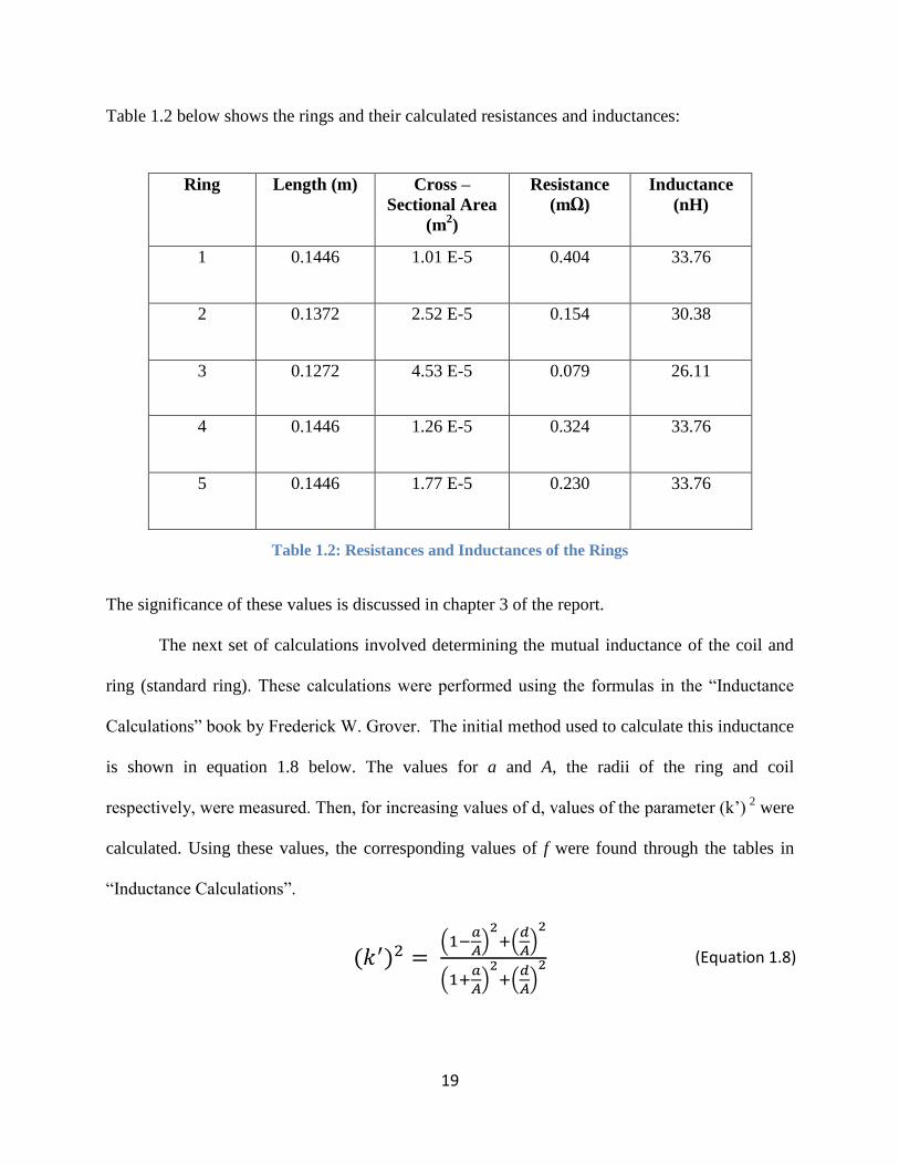
(Equation 1.8)
Table 1.2 below shows the rings and their calculated resistances and inductances:
Table 1.2: Resistances and Inductances of the Rings
The significance of these values is discussed in chapter 3 of the report.
The next set of calculations involved determining the mutual inductance of the coil and
ring (standard ring). These calculations were performed using the formulas in the “Inductance
Calculations” book by Frederick W. Grover. The initial method used to calculate this inductance
is shown in equation 1.8 below. The values for a and A, the radii of the ring and coil
respectively, were measured. Then, for increasing values of d, values of the parameter (k’) 2
were
calculated. Using these values, the corresponding values of f were found through the tables in
“Inductance Calculations”.
( ) (
) (
)
(
) (
)
Ring Length (m) Cross –
Sectional Area
(m2)
Resistance
(mΩ)
Inductance
(nH)
1 0.1446 1.01 E-5 0.404 33.76
2 0.1372 2.52 E-5 0.154 30.38
3 0.1272 4.53 E-5 0.079 26.11
4 0.1446 1.26 E-5 0.324 33.76
5 0.1446 1.77 E-5 0.230 33.76

20
(Equation 1.9)
0
0.005
0.01
0.015
0.02
0.025
0.03
0.035
0.04
0 2 4 6 8 10 12Mu
tual
Ind
uct
ance
bet
wee
n C
oil
and
Rin
g (µ
H)
Distance between Coil and Ring (cm)
Mutual Inductance vs Distance
The calculation of the mutual inductance was then performed using equation 1.9 and the
mutual inductance was then graphed against distance, as shown in figure 1.10. These calculations
and the corresponding graph were all done using Microsoft Excel
√
While the mutual inductance calculated using the equations above is correct, a more
accurate method of calculating mutual inductance is through the Lyle Method. The Lyle Method
involves replacing the coil or ring with two filaments, 1 and 2, and the distance apart of the
filaments being the equivalent breadth, 2β, of the coil.
Figure 1.10: Mutual Inductance vs Distance graph

21
(Equation 1.10)
(Equation 1.11)
(Equation 1.12)
The value of β was calculated using the following equation:
The equivalent radius of A was calculated using equation 1.11:
(
)
Using the formulae above, the coil and ring were broken down into two filaments each,
with four different radii. The mutual inductance, using the Lyle Method, is the sum of the mutual
inductances between the four filaments, multiplied by the number of turns in the coil (50) and the
number of turns in the ring (1). The equation is shown below:
In equation 1.12, Mo is the sum of the mutual inductances of M13, M14, M23 and M24. The
calculations using the Lyle Method formed a much more accurate graph on excel, shown in
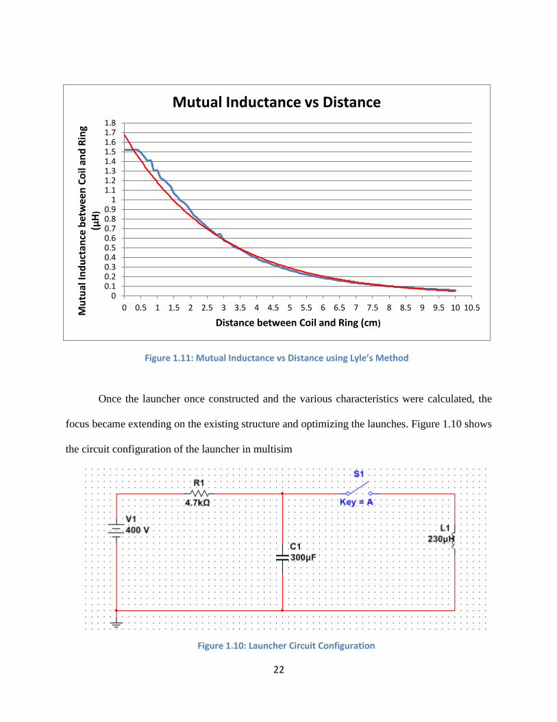
figure 1.11. The full set of values calculated for this graph can be found in Appendix B.
According to the graph, the maximum value of the mutual inductance was found to be 1.52µH
for a distance of 0 to 0.4cm. Theoretically the maximum value for mutual inductance should be
at 0 cm only. This slight error is due to the Lyle Method being based on numerous
approximations.
22
00.10.20.30.40.50.60.70.80.9
11.11.21.31.41.51.61.71.8
0 0.5 1 1.5 2 2.5 3 3.5 4 4.5 5 5.5 6 6.5 7 7.5 8 8.5 9 9.5 10 10.5Mu
tual
Ind
uct
ance
bet
wee
n C
oil
and
Rin
g (µ
H)
Distance between Coil and Ring (cm)
Mutual Inductance vs Distance
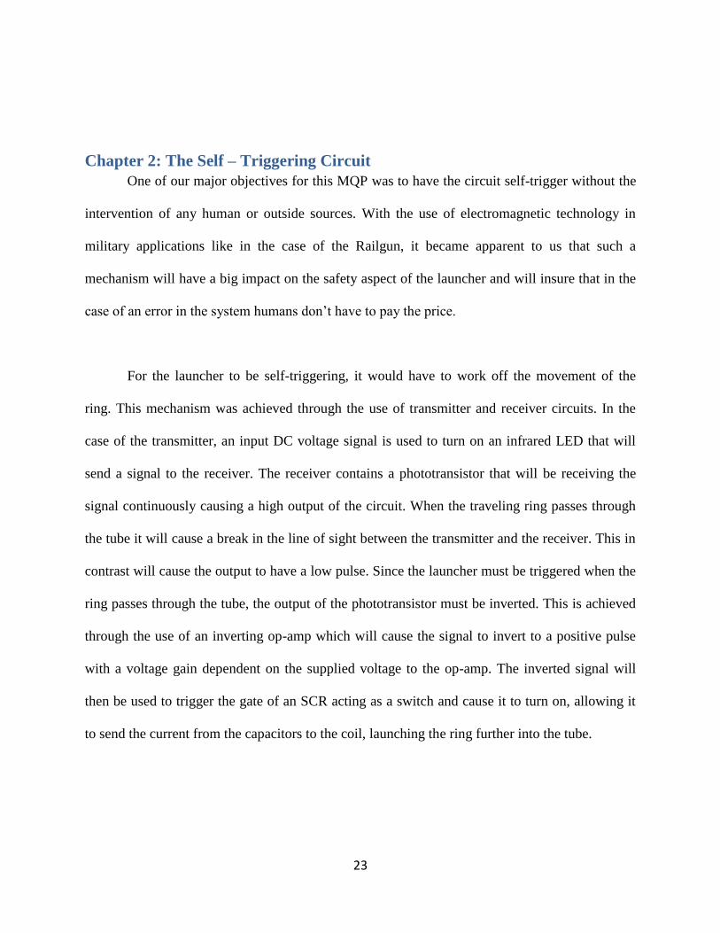
Once the launcher once constructed and the various characteristics were calculated, the
focus became extending on the existing structure and optimizing the launches. Figure 1.10 shows
the circuit configuration of the launcher in multisim
Figure 1.10: Launcher Circuit Configuration
Figure 1.11: Mutual Inductance vs Distance using Lyle’s Method
23
Chapter 2: The Self – Triggering Circuit
One of our major objectives for this MQP was to have the circuit self-trigger without the
intervention of any human or outside sources. With the use of electromagnetic technology in
military applications like in the case of the Railgun, it became apparent to us that such a
mechanism will have a big impact on the safety aspect of the launcher and will insure that in the
case of an error in the system humans don’t have to pay the price.
For the launcher to be self-triggering, it would have to work off the movement of the
ring. This mechanism was achieved through the use of transmitter and receiver circuits. In the
case of the transmitter, an input DC voltage signal is used to turn on an infrared LED that will
send a signal to the receiver. The receiver contains a phototransistor that will be receiving the
signal continuously causing a high output of the circuit. When the traveling ring passes through
the tube it will cause a break in the line of sight between the transmitter and the receiver. This in
contrast will cause the output to have a low pulse. Since the launcher must be triggered when the
ring passes through the tube, the output of the phototransistor must be inverted. This is achieved
through the use of an inverting op-amp which will cause the signal to invert to a positive pulse
with a voltage gain dependent on the supplied voltage to the op-amp. The inverted signal will
then be used to trigger the gate of an SCR acting as a switch and cause it to turn on, allowing it
to send the current from the capacitors to the coil, launching the ring further into the tube.
24
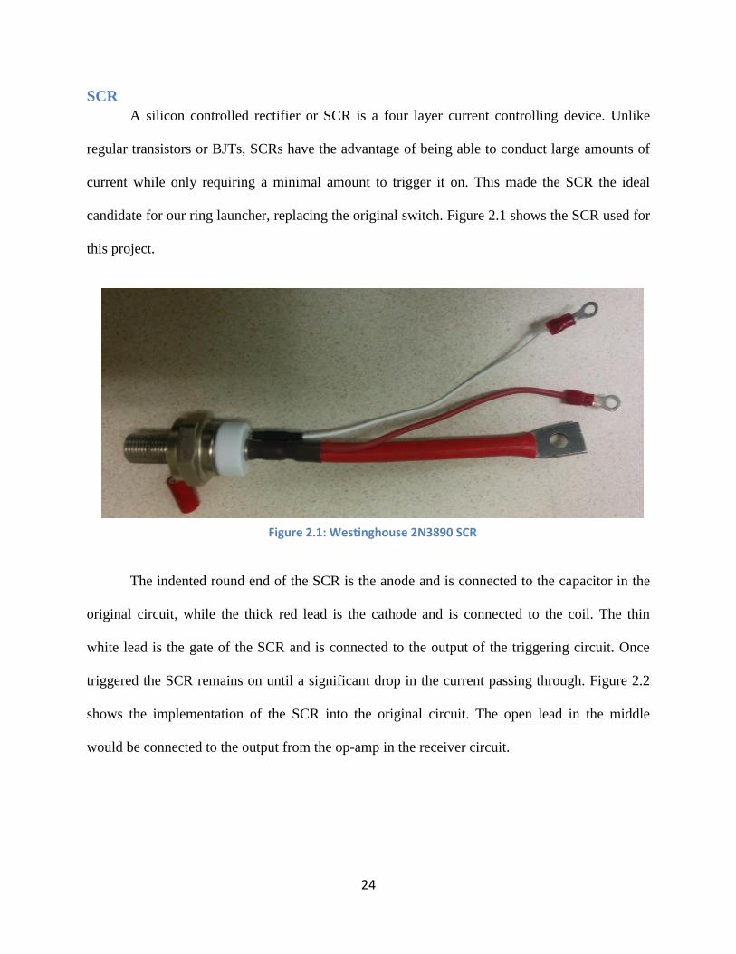
SCR
A silicon controlled rectifier or SCR is a four layer current controlling device. Unlike
regular transistors or BJTs, SCRs have the advantage of being able to conduct large amounts of
current while only requiring a minimal amount to trigger it on. This made the SCR the ideal
candidate for our ring launcher, replacing the original switch. Figure 2.1 shows the SCR used for
this project.
The indented round end of the SCR is the anode and is connected to the capacitor in the
original circuit, while the thick red lead is the cathode and is connected to the coil. The thin
white lead is the gate of the SCR and is connected to the output of the triggering circuit. Once
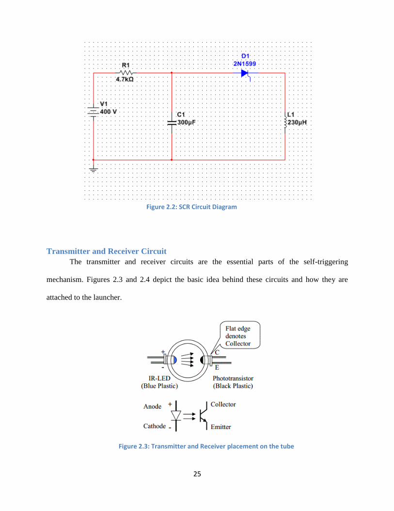
triggered the SCR remains on until a significant drop in the current passing through. Figure 2.2
shows the implementation of the SCR into the original circuit. The open lead in the middle
would be connected to the output from the op-amp in the receiver circuit.
Figure 2.1: Westinghouse 2N3890 SCR
25
Transmitter and Receiver Circuit
The transmitter and receiver circuits are the essential parts of the self-triggering
mechanism. Figures 2.3 and 2.4 depict the basic idea behind these circuits and how they are
attached to the launcher.
Figure 2.2: SCR Circuit Diagram
Figure 2.3: Transmitter and Receiver placement on the tube

26
As shown in the diagrams above the circuit’s functionality is based upon the interaction
between the infrared LED and infrared phototransistor. This works perfectly for the requirement
of a self-triggering mechanism since it can be based around the movement of a projectile, such as
a ring. The LED transmitter circuit can be attached on one end of the tube as shown in figure 2.3
and the receiver on the opposite end with the phototransistor facing the LED. Normally, the LED
transmits photons to the phototransistor which converts this to a current. If an oscilloscope is
attached to the output like in figure 2.4, it would display a small positive reading. However, for
the transmitter and receiver to be constantly configured and to the have the mechanism only be
triggered by the movement of the ring, the output has to be attached to the gate of the SCR
somehow. Since this is a very small output value it will not trigger the gate of the SCR.
As the ring passes through the tube, it will momentarily block the line of sight between
the LED and phototransistor. To have the trigger be based on the ring’s motion, this is the point
in time when the SCR should be switched on and by having the coil attached to the tube just
Figure 2.4: Transmitter and Receiver Circuit Configurations
27
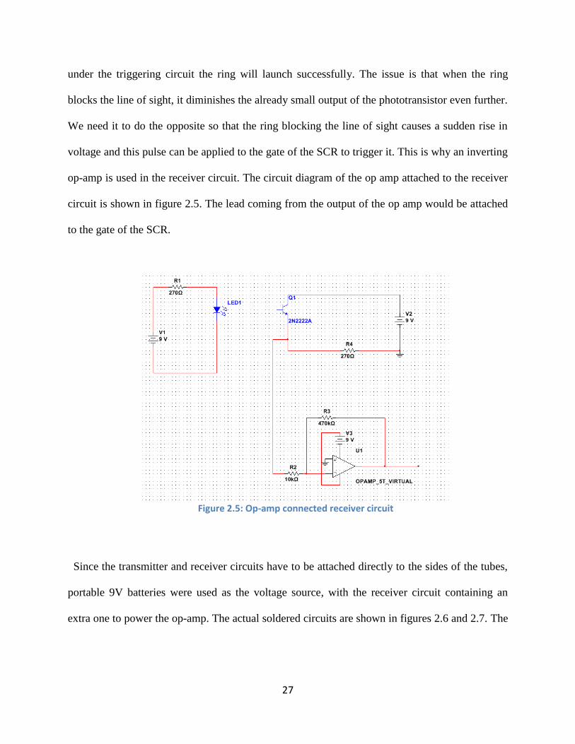
under the triggering circuit the ring will launch successfully. The issue is that when the ring
blocks the line of sight, it diminishes the already small output of the phototransistor even further.
We need it to do the opposite so that the ring blocking the line of sight causes a sudden rise in
voltage and this pulse can be applied to the gate of the SCR to trigger it. This is why an inverting
op-amp is used in the receiver circuit. The circuit diagram of the op amp attached to the receiver
circuit is shown in figure 2.5. The lead coming from the output of the op amp would be attached
to the gate of the SCR.
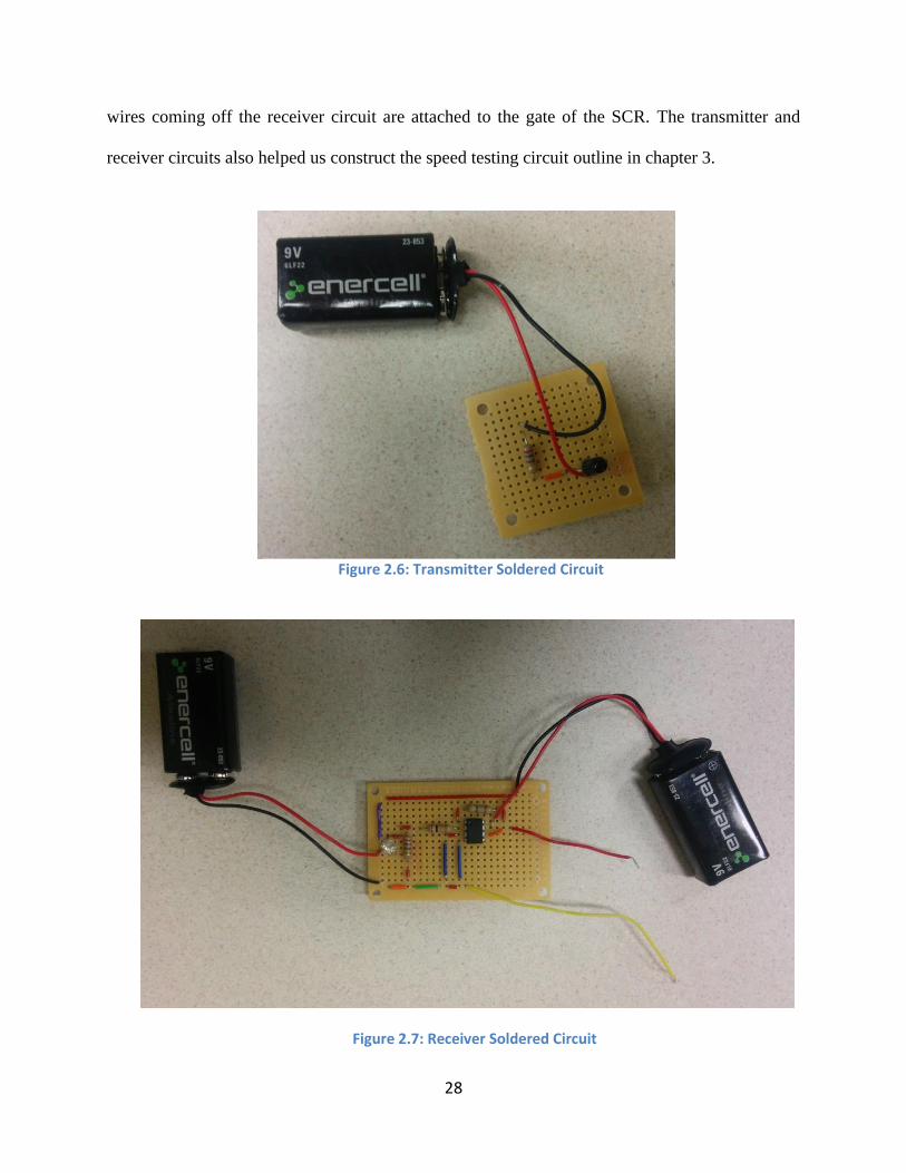
Since the transmitter and receiver circuits have to be attached directly to the sides of the tubes,
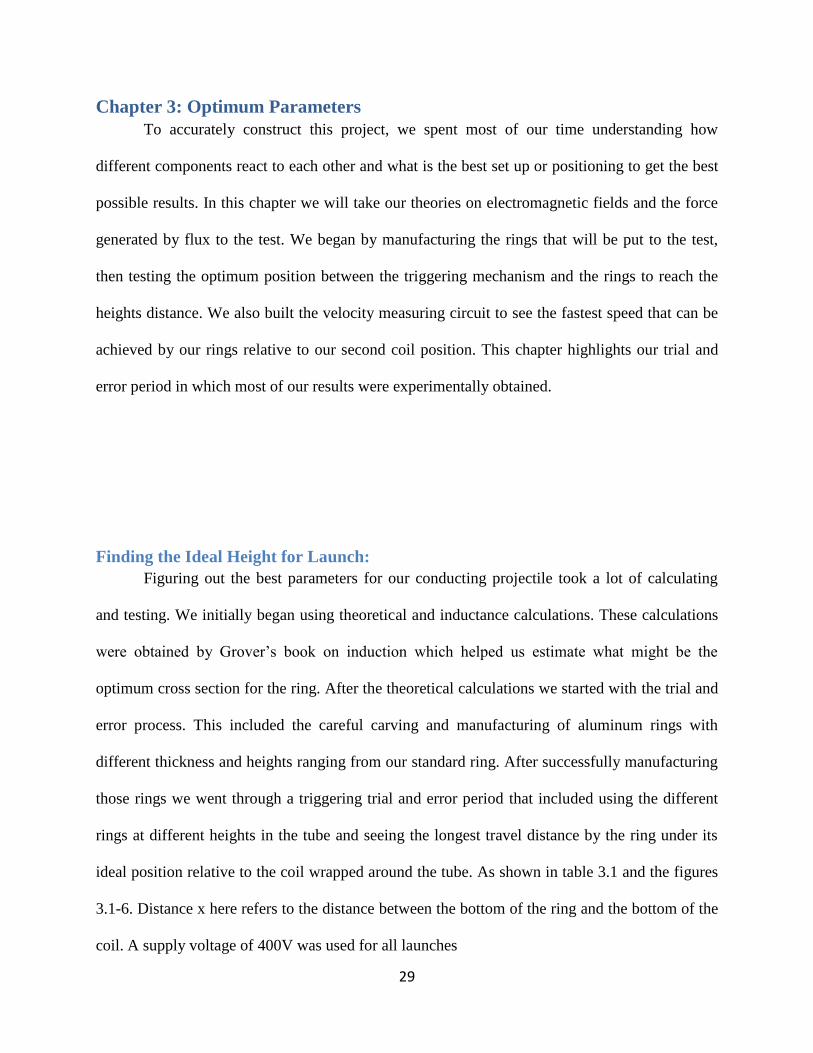
portable 9V batteries were used as the voltage source, with the receiver circuit containing an
extra one to power the op-amp. The actual soldered circuits are shown in figures 2.6 and 2.7. The
Figure 2.5: Op-amp connected receiver circuit
28
wires coming off the receiver circuit are attached to the gate of the SCR. The transmitter and
receiver circuits also helped us construct the speed testing circuit outline in chapter 3.
Figure 2.6: Transmitter Soldered Circuit
Figure 2.7: Receiver Soldered Circuit
29
Chapter 3: Optimum Parameters
To accurately construct this project, we spent most of our time understanding how
different components react to each other and what is the best set up or positioning to get the best
possible results. In this chapter we will take our theories on electromagnetic fields and the force
generated by flux to the test. We began by manufacturing the rings that will be put to the test,
then testing the optimum position between the triggering mechanism and the rings to reach the
heights distance. We also built the velocity measuring circuit to see the fastest speed that can be
achieved by our rings relative to our second coil position. This chapter highlights our trial and
error period in which most of our results were experimentally obtained.
Finding the Ideal Height for Launch:
Figuring out the best parameters for our conducting projectile took a lot of calculating
and testing. We initially began using theoretical and inductance calculations. These calculations
were obtained by Grover’s book on induction which helped us estimate what might be the
optimum cross section for the ring. After the theoretical calculations we started with the trial and
error process. This included the careful carving and manufacturing of aluminum rings with
different thickness and heights ranging from our standard ring. After successfully manufacturing
those rings we went through a triggering trial and error period that included using the different
rings at different heights in the tube and seeing the longest travel distance by the ring under its
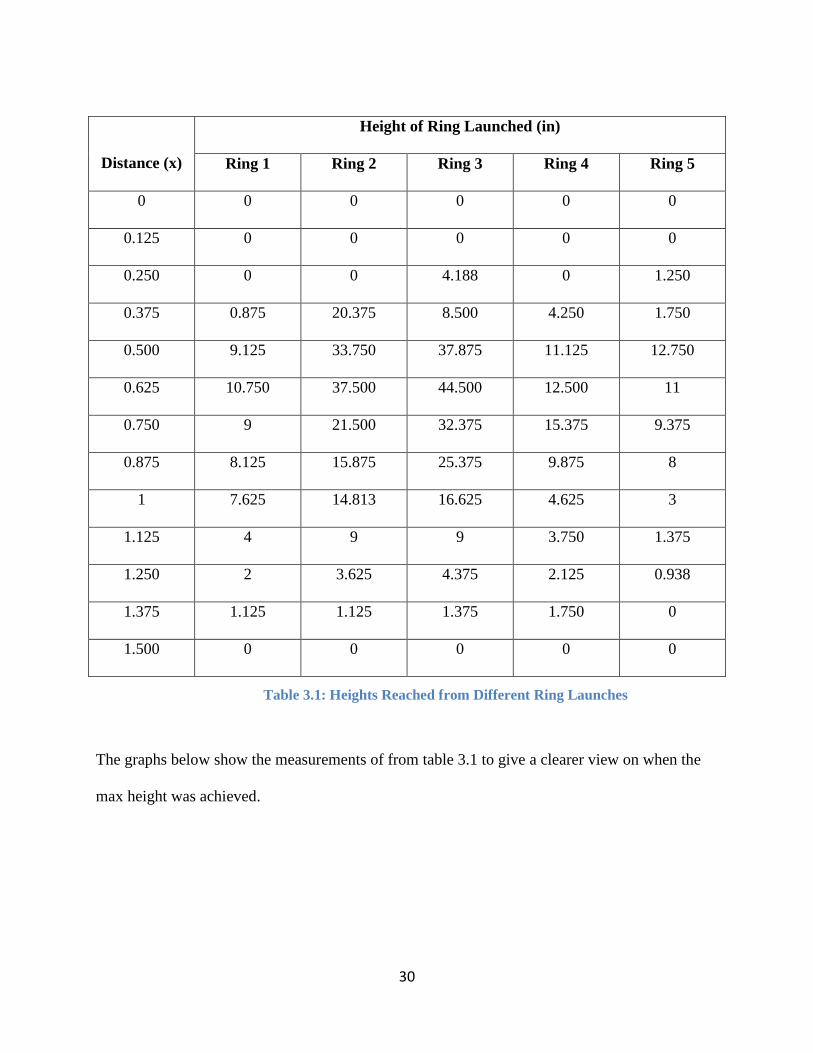
ideal position relative to the coil wrapped around the tube. As shown in table 3.1 and the figures
3.1-6. Distance x here refers to the distance between the bottom of the ring and the bottom of the
coil. A supply voltage of 400V was used for all launches
30
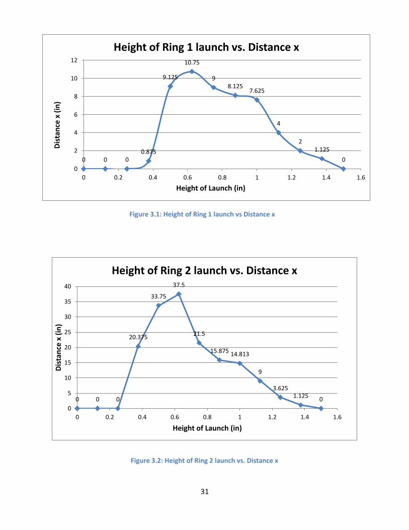
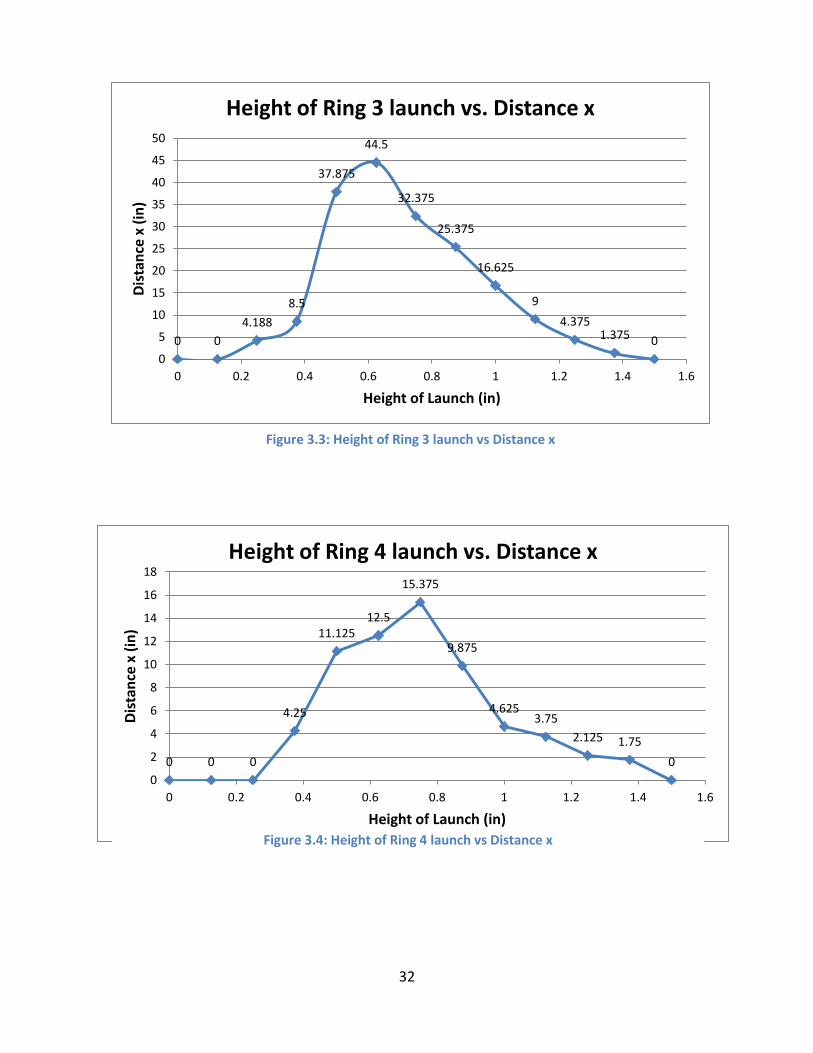
The graphs below show the measurements of from table 3.1 to give a clearer view on when the
max height was achieved.
Distance (x)
Height of Ring Launched (in)
Ring 1 Ring 2 Ring 3 Ring 4 Ring 5
0 0 0 0 0 0
0.125 0 0 0 0 0
0.250 0 0 4.188 0 1.250
0.375 0.875 20.375 8.500 4.250 1.750
0.500 9.125 33.750 37.875 11.125 12.750
0.625 10.750 37.500 44.500 12.500 11
0.750 9 21.500 32.375 15.375 9.375
0.875 8.125 15.875 25.375 9.875 8
1 7.625 14.813 16.625 4.625 3
1.125 4 9 9 3.750 1.375
1.250 2 3.625 4.375 2.125 0.938
1.375 1.125 1.125 1.375 1.750 0
1.500 0 0 0 0 0
Table 3.1: Heights Reached from Different Ring Launches
31
0 0 0 0.875
9.125
10.75
9 8.125
7.625
4
2 1.125
0
0
2
4
6
8
10
12
0 0.2 0.4 0.6 0.8 1 1.2 1.4 1.6
Dis
tan
ce x
(in
)
Height of Launch (in)
Height of Ring 1 launch vs. Distance x
0 0 0
20.375
33.75
37.5
21.5
15.875 14.813
9
3.625 1.125
0
0
5
10
15
20
25
30
35
40
0 0.2 0.4 0.6 0.8 1 1.2 1.4 1.6
Dis
tan
ce x
(in
)
Height of Launch (in)
Height of Ring 2 launch vs. Distance x
Figure 3.2: Height of Ring 2 launch vs. Distance x
Figure 3.1: Height of Ring 1 launch vs Distance x
32
0 0
4.188
8.5
37.875
44.5
32.375
25.375
16.625
9
4.375 1.375 0
0
5
10
15
20
25
30
35
40
45
50
0 0.2 0.4 0.6 0.8 1 1.2 1.4 1.6
Dis
tan
ce x
(in
)
Height of Launch (in)
Height of Ring 3 launch vs. Distance x
0 0 0
4.25
11.125 12.5
15.375
9.875
4.625 3.75
2.125 1.75
0
0
2
4
6
8
10
12
14
16
18
0 0.2 0.4 0.6 0.8 1 1.2 1.4 1.6
Dis
tan
ce x
(in
)
Height of Launch (in)
Height of Ring 4 launch vs. Distance x
Figure 3.4: Height of Ring 4 launch vs Distance x
Figure 3.3: Height of Ring 3 launch vs Distance x

33
0 0
1.25 1.75
12.75
11
9.375
8
3
1.375 0.938
0 0
0
2
4
6
8
10
12
14
0 0.2 0.4 0.6 0.8 1 1.2 1.4 1.6
Dis
tan
ce x
(in
)
Height of Launch (in)
Height of Ring 5 launch vs. Distance x
The results from the graphs above were used to find the ideal distance x between the
bottom of the coil and the bottom of the ring. This distance was found to be 0.625 in. The
different rings were then tested at this height to compare the launch heights achieved by each
ring. The results are shown in figure 3.6 below
Figure 3.5: Height of Ring 5 launch vs Distance x

34
10.75
37.5
44.5
15.375 12.75
0
5
10
15
20
25
30
35
40
45
50
Max
Lau
nch
Hei
ght
(in
)
Max Launch Height of Rings
Ring 1 Ring 2 Ring 3 Ring 4 Ring 5
The graph above shows that the ideal ring from testing that achieved the highest launch
was ring 3. This validates the resistance calculations from chapter 1 that showed ring 3 to have
the lowest resistance. A lower resistance would mean a higher current induced in the ring,
allowing it to travel further up the tube.
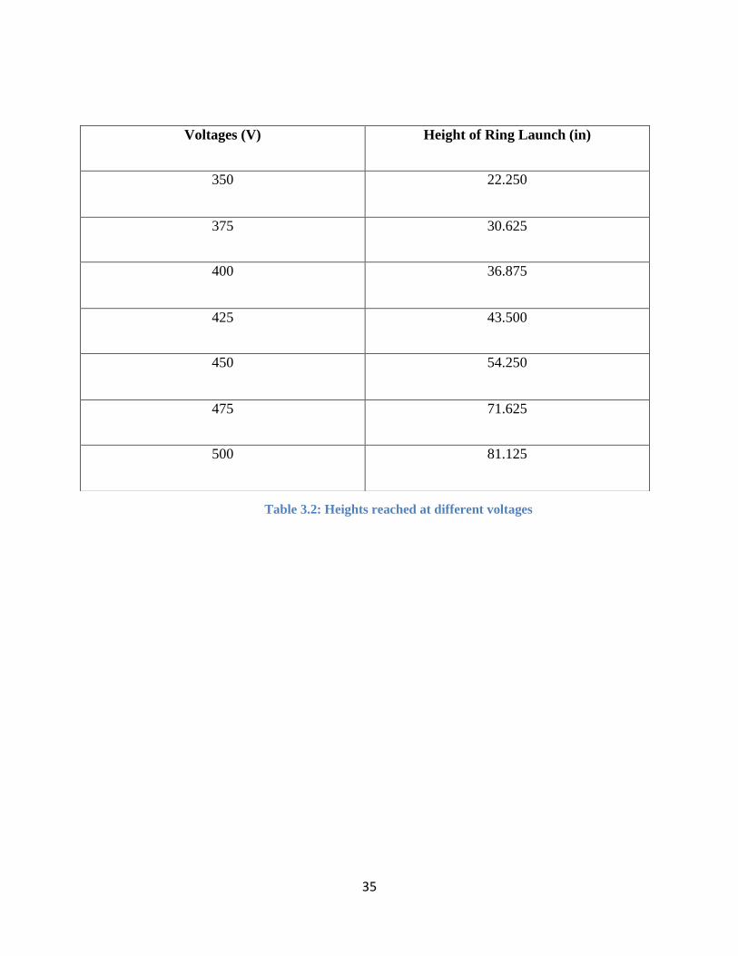
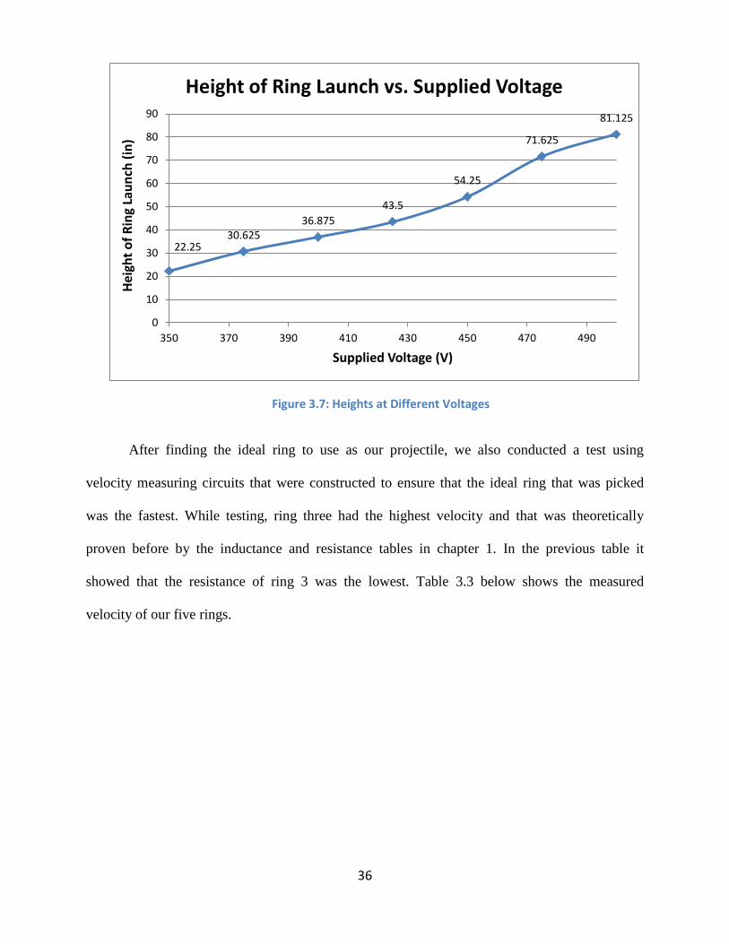
After finding idea ring shown in the graphs above, we began experimenting with different
voltages like in our simulation in PSpice. The power supply used ranged from 350-500 volts and
we tested these voltages at increments of 25 volts. Using 500 volts gave us the highest launch of
our ideal ring as predicted using Faraday’s law. Figure 3.7 and Table 3.2 below shows the test
results.
Figure 3.6: Comparison of Max Heights Reached by Rings
35
Voltages (V) Height of Ring Launch (in)
350 22.250
375 30.625
400 36.875
425 43.500
450 54.250
475 71.625
500 81.125
Table 3.2: Heights reached at different voltages
36
22.25 30.625
36.875
43.5
54.25
71.625
81.125
0
10
20
30
40
50
60
70
80
90
350 370 390 410 430 450 470 490
Hei
ght
of
Rin
g La
un
ch (
in)
Supplied Voltage (V)
Height of Ring Launch vs. Supplied Voltage
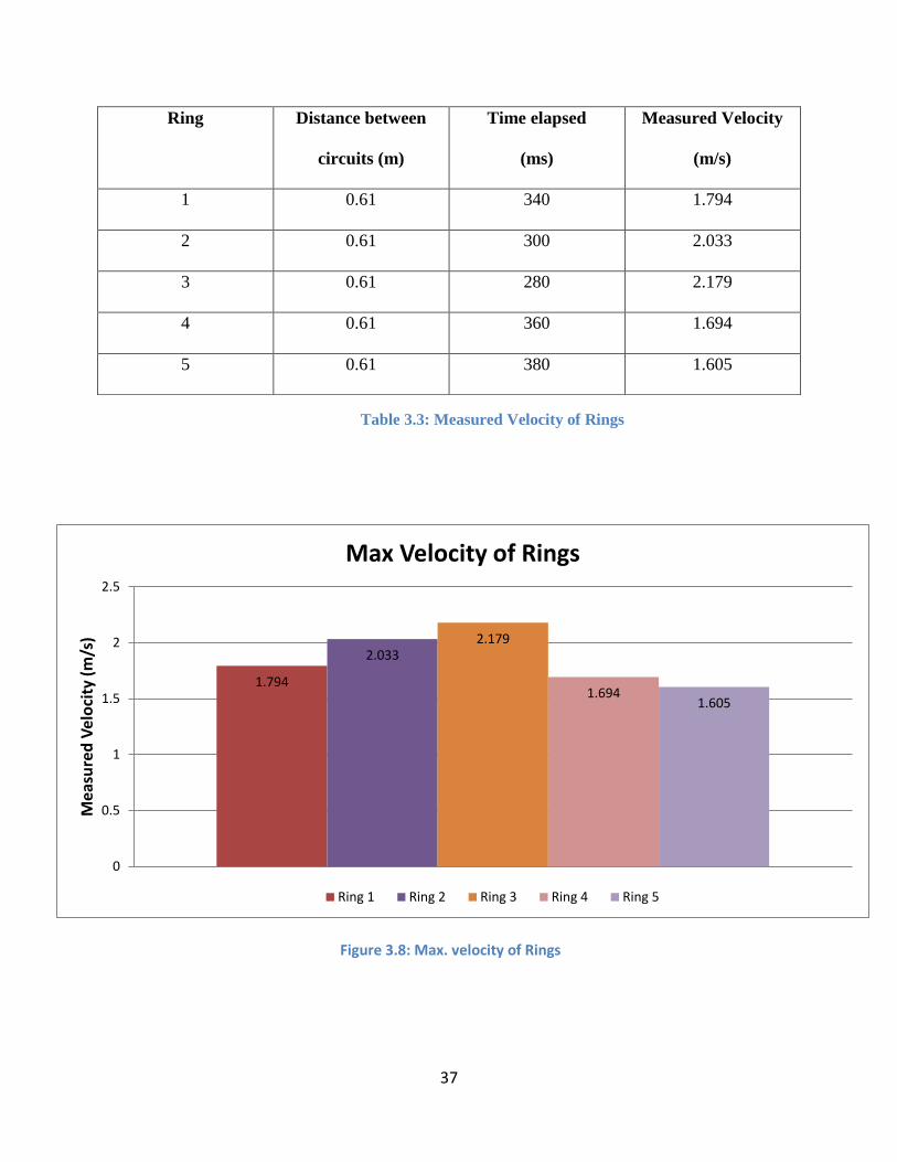
After finding the ideal ring to use as our projectile, we also conducted a test using
velocity measuring circuits that were constructed to ensure that the ideal ring that was picked
was the fastest. While testing, ring three had the highest velocity and that was theoretically
proven before by the inductance and resistance tables in chapter 1. In the previous table it
showed that the resistance of ring 3 was the lowest. Table 3.3 below shows the measured
velocity of our five rings.
Figure 3.7: Heights at Different Voltages
37
1.794
2.033 2.179
1.694 1.605
0
0.5
1
1.5
2
2.5
Mea
sure
d V
elo
city
(m
/s)
Max Velocity of Rings
Ring 1 Ring 2 Ring 3 Ring 4 Ring 5
Ring Distance between
circuits (m)
Time elapsed
(ms)
Measured Velocity
(m/s)
1 0.61 340 1.794
2 0.61 300 2.033
3 0.61 280 2.179
4 0.61 360 1.694
5 0.61 380 1.605
Table 3.3: Measured Velocity of Rings
Figure 3.8: Max. velocity of Rings
38
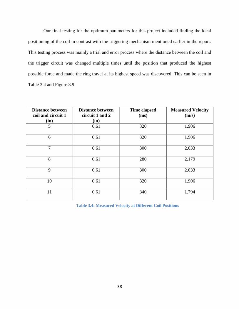
Our final testing for the optimum parameters for this project included finding the ideal
positioning of the coil in contrast with the triggering mechanism mentioned earlier in the report.
This testing process was mainly a trial and error process where the distance between the coil and
the trigger circuit was changed multiple times until the position that produced the highest
possible force and made the ring travel at its highest speed was discovered. This can be seen in
Table 3.4 and Figure 3.9.
Distance between
coil and circuit 1
(in)
Distance between
circuit 1 and 2
(in)
Time elapsed
(ms)
Measured Velocity
(m/s)
5 0.61 320 1.906
6 0.61 320 1.906
7 0.61 300 2.033
8 0.61 280 2.179
9 0.61 300 2.033
10 0.61 320 1.906
11 0.61 340 1.794
Table 3.4: Measured Velocity at Different Coil Positions

39
1.906 1.906 2.033
2.179
2.033 1.906
1.794
0
0.5
1
1.5
2
2.5
3
5 6 7 8 9 10 11
Mea
sure
d V
elo
city
(m
/s)
Distance between coil and circuit 1 (in)
Measured Velocity
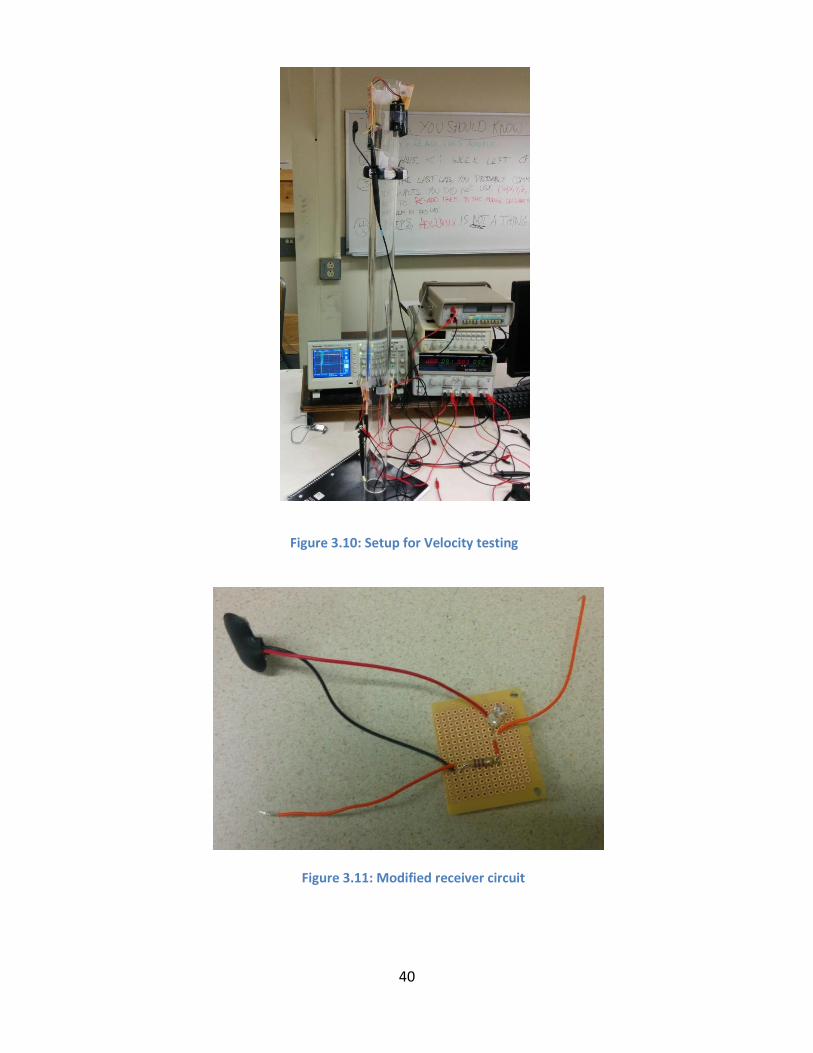
Speed testing circuit:
The velocity tests conducted in this chapter were done through the use of an extended
transmitter and receiver circuit first introduced in chapter 2. The speed circuit was used to
measure the ideal position for the coil relative to the triggering circuit and was used to reconfirm
the ideal ring found from the height experiments did in fact travel the fastest through the tube.
The set up for this circuit was parallel to the triggering circuit further above the tube. It also uses
an LED transmitter and a receiver. But unlike the triggering circuit it does not contain an
inverting op-amp as the output from the phototransistor simply needs to be monitored for a
change when the ring passes and is not used as a voltage source for a separate circuit. When the
ring passes through the tube it creates two consecutive pulses; one on the output of the triggering
circuit’s phototransistor and another on the output of the speed circuit’s phototransistor.
Knowing the distance between these two circuits and the time elapsed between the pulses on an
oscilloscope, the velocity can be measured. The setup for this velocity testing and the modified
receiver circuit can be seen in figures 3.10 and 3.11 below
Figure 3.9: Measured Velocity at Different Coil Positions
40
Figure 3.10: Setup for Velocity testing
Figure 3.11: Modified receiver circuit
41
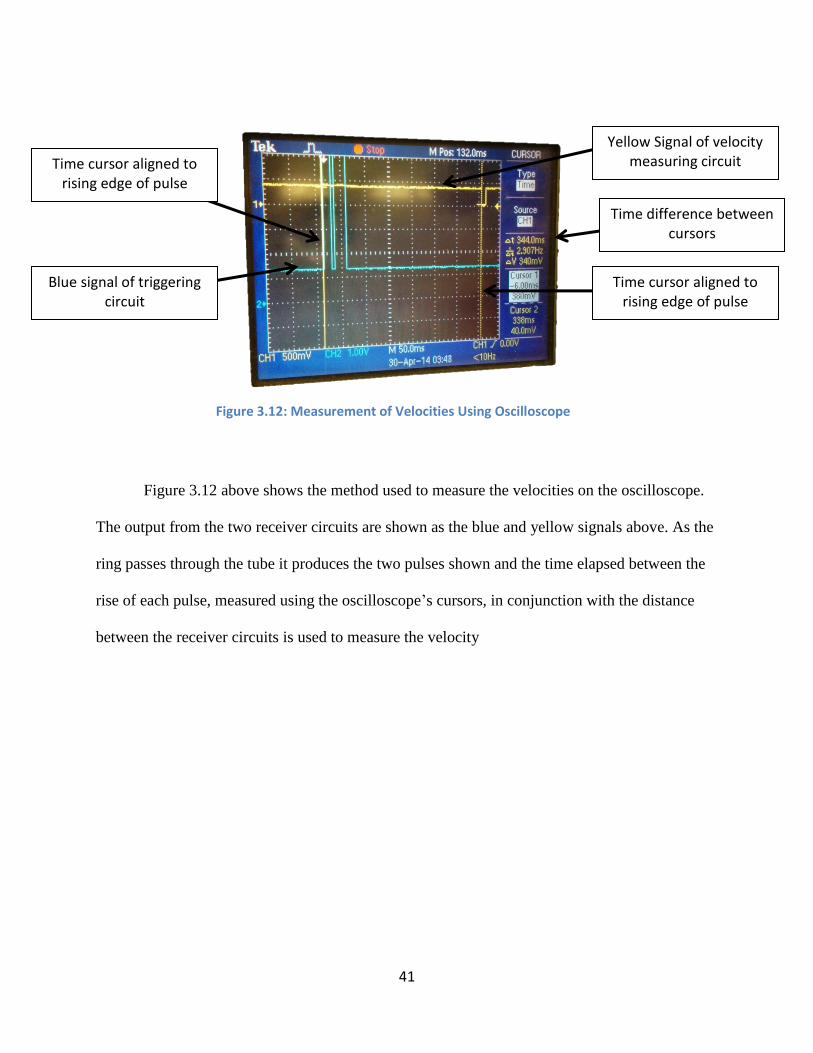
Figure 3.12 above shows the method used to measure the velocities on the oscilloscope.
The output from the two receiver circuits are shown as the blue and yellow signals above. As the
ring passes through the tube it produces the two pulses shown and the time elapsed between the
rise of each pulse, measured using the oscilloscope’s cursors, in conjunction with the distance
between the receiver circuits is used to measure the velocity
Figure 3.12: Measurement of Velocities Using Oscilloscope
Time cursor aligned to rising edge of pulse
Time cursor aligned to rising edge of pulse
Time difference between cursors
Yellow Signal of velocity measuring circuit
Blue signal of triggering circuit
42
Chapter 4 – Project Simulation
PSpice Simulation
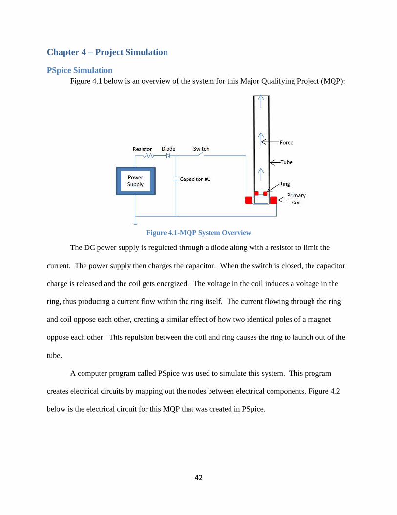
Figure 4.1 below is an overview of the system for this Major Qualifying Project (MQP):
Figure 4.1-MQP System Overview
The DC power supply is regulated through a diode along with a resistor to limit the
current. The power supply then charges the capacitor. When the switch is closed, the capacitor
charge is released and the coil gets energized. The voltage in the coil induces a voltage in the
ring, thus producing a current flow within the ring itself. The current flowing through the ring
and coil oppose each other, creating a similar effect of how two identical poles of a magnet
oppose each other. This repulsion between the coil and ring causes the ring to launch out of the
tube.
A computer program called PSpice was used to simulate this system. This program
creates electrical circuits by mapping out the nodes between electrical components. Figure 4.2
below is the electrical circuit for this MQP that was created in PSpice.

43
Figure 4.2-PSpice Electrical Circuit
Figure 4.2a above consists of two circuits. The left circuit represents the coil and has the
following voltage loop equation:
∫
The circuit on the right presents the ring as has the following voltage loop equation:
The simulation took in effect that the capacitor C was fully charged to 500V so the diode
and resistor connected to the source were not needed in the simulation. The capacitor has a
capacitance of 300µF.
A) Electrical
System
B) Integrator
that yields
current
values
∫
44
(Eq. 4.1)
(Eq. 4.2)
(Eq. 4.3)
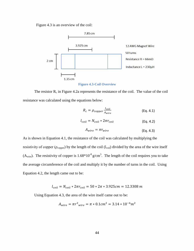
Figure 4.3 is an overview of the coil:
Figure 4.3-Coil Overview
The resistor Rc in Figure 4.2a represents the resistance of the coil. The value of the coil
resistance was calculated using the equations below:
As is shown in Equation 4.1, the resistance of the coil was calculated by multiplying the
resistivity of copper (ρcopper) by the length of the coil (lcoil) divided by the area of the wire itself
(Awire). The resistivity of copper is 1.68*10-8
g/cm3. The length of the coil requires you to take
the average circumference of the coil and multiply it by the number of turns in the coil. Using
Equation 4.2, the length came out to be:
Using Equation 4.3, the area of the wire itself came out to be:
45
(Eq. 4.4)
Putting all of these values back into Equation 4.1, the resistance came out to be:
( )
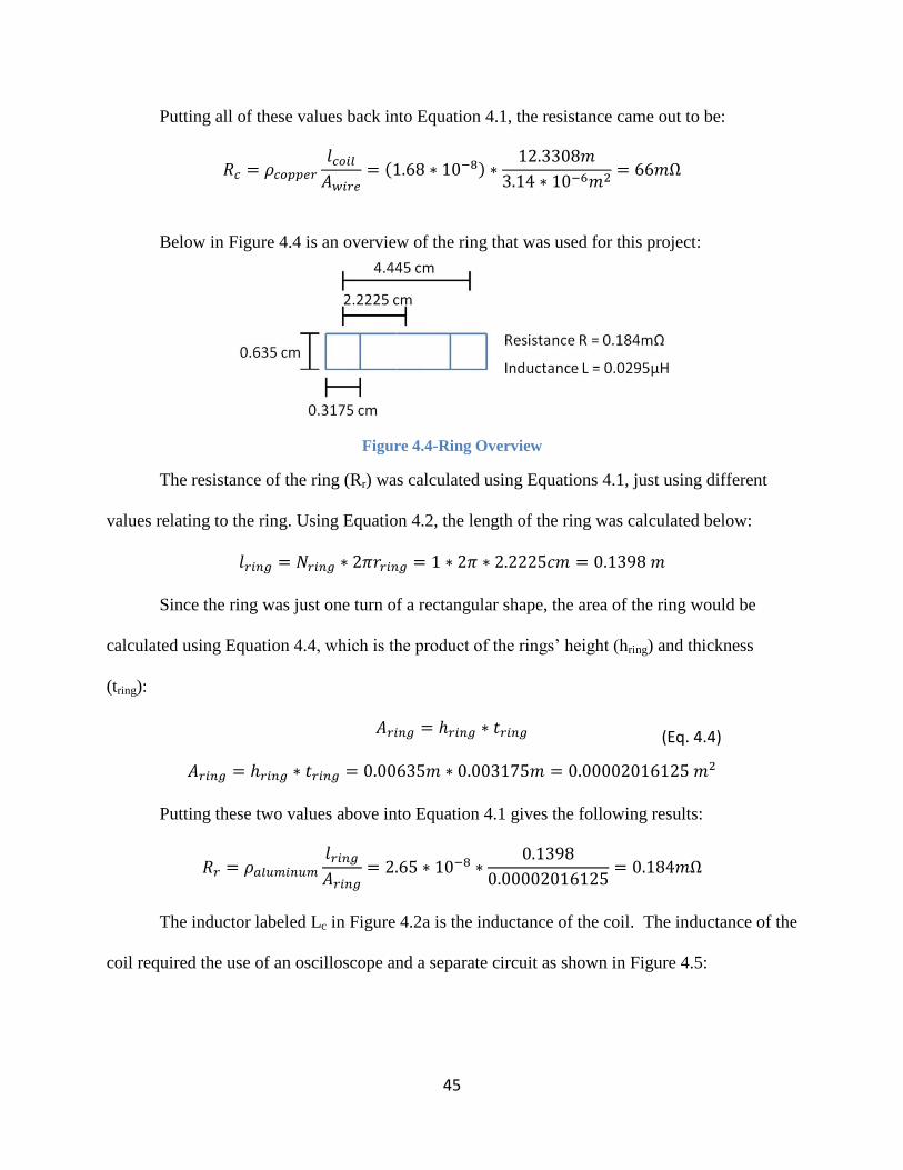
Below in Figure 4.4 is an overview of the ring that was used for this project:
Figure 4.4-Ring Overview
The resistance of the ring (Rr) was calculated using Equations 4.1, just using different
values relating to the ring. Using Equation 4.2, the length of the ring was calculated below:
Since the ring was just one turn of a rectangular shape, the area of the ring would be
calculated using Equation 4.4, which is the product of the rings’ height (hring) and thickness
(tring):
Putting these two values above into Equation 4.1 gives the following results:
The inductor labeled Lc in Figure 4.2a is the inductance of the coil. The inductance of the
coil required the use of an oscilloscope and a separate circuit as shown in Figure 4.5:
46
(Eq. 4.5)
(Eq. 4.6)
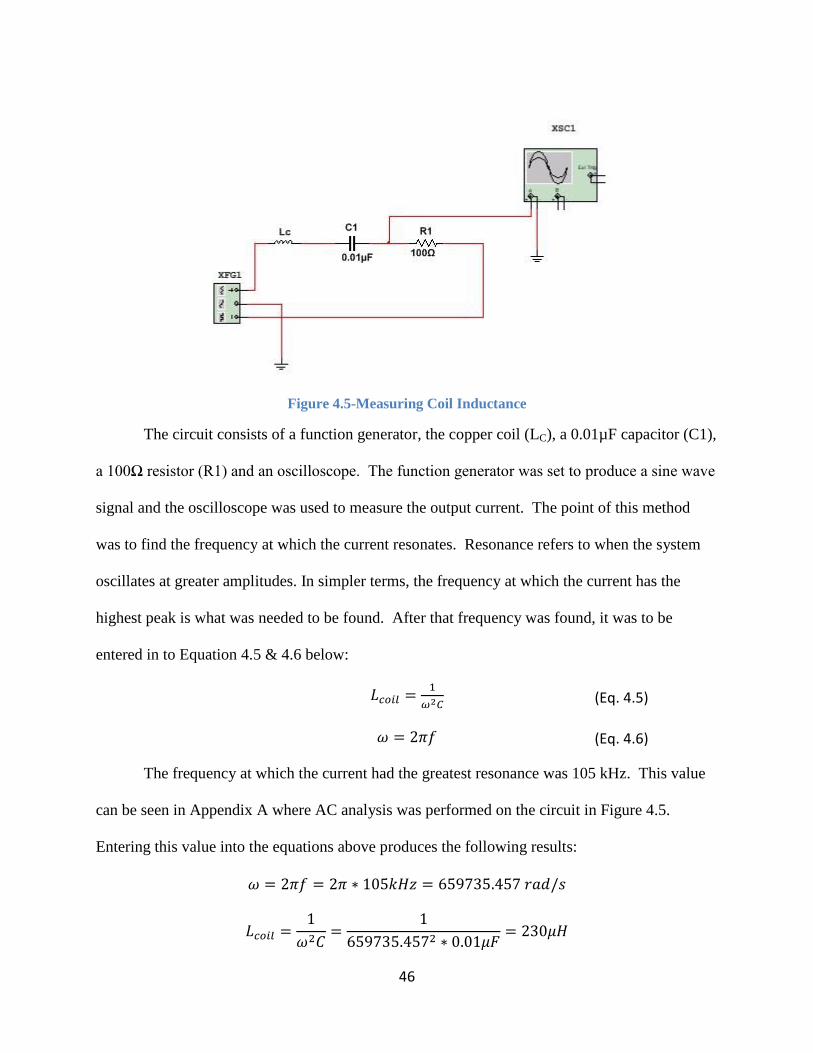
Figure 4.5-Measuring Coil Inductance
The circuit consists of a function generator, the copper coil (LC), a 0.01µF capacitor (C1),
a 100Ω resistor (R1) and an oscilloscope. The function generator was set to produce a sine wave
signal and the oscilloscope was used to measure the output current. The point of this method
was to find the frequency at which the current resonates. Resonance refers to when the system
oscillates at greater amplitudes. In simpler terms, the frequency at which the current has the
highest peak is what was needed to be found. After that frequency was found, it was to be
entered in to Equation 4.5 & 4.6 below:
The frequency at which the current had the greatest resonance was 105 kHz. This value
can be seen in Appendix A where AC analysis was performed on the circuit in Figure 4.5.
Entering this value into the equations above produces the following results:
47
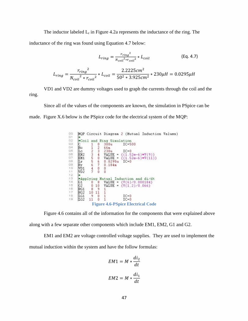
(Eq. 4.7)
The inductor labeled Lr in Figure 4.2a represents the inductance of the ring. The
inductance of the ring was found using Equation 4.7 below:
VD1 and VD2 are dummy voltages used to graph the currents through the coil and the
ring.
Since all of the values of the components are known, the simulation in PSpice can be
made. Figure X.6 below is the PSpice code for the electrical system of the MQP:
Figure 4.6-PSpice Electrical Code
Figure 4.6 contains all of the information for the components that were explained above
along with a few separate other components which include EM1, EM2, G1 and G2.
EM1 and EM2 are voltage controlled voltage supplies. They are used to implement the
mutual induction within the system and have the follow formulas:

48
The symbol M stands for Mutual Inductance which is the inductance created between the
coil and ring. As seen in Figure 4.6 and previously shown in Chapter 1, the mutual induction is
1.52µH.
The values for
and
are found using the voltage controlled current sources G1 and
G2 that are seen in Figure X.2b. As seen in Figure 4.6, G1 has the following value:
( )
The value V(6) stands for the voltage at Node 6 of the circuit shown in Figure X.2. The
value 0.000184 is the resistance of the ring. Together these two values are used to find the
current flowing through the ring, which is the value of G1.
Also from Figure X.6, G2 has the following value:
( )
The value V(1,2) is the voltage between nodes 1 and 2 in the circuit shown in Figure X.2.
The resistance of the coil is represented by the value 0.066. Together these values are used to
find the current in the coil, which is the value of G2.
Running the simulation, the following graphs were produced:
Figure 4.7-Ring and Coil Currents vs. Time
A) Current through
ring
B) Current through
coil

49
Figure 4.7A represents the current going through the ring which is around 12k amps.
Figure 4.7B represents the current in the coil which is about 500 amps. This is exactly what is
needed for this system. The current through the ring is a lot higher than the current in the coil
because the ring coil is going through only one turn while the coil have 50 turns that the current
has to go through. The greater the current through the ring, the greater the opposing forces
between the ring and coil will be.
Optimizing the System – Force, Velocity, and Height
In order to optimize the system to produce the greatest force, velocity and height, the best
position for the ring to be at was to be found. This process required the use of the following
diagram:
Figure 4.8-Optimizing the System (Resultant Force Calculations)
In Figure 4.8, the bottom block represents the coil and the top block represents the ring.
The distance between the coil and ring centers is h, k is the difference between the radius of the
coil and the radius of the ring, δ is the diagonal distance between the coil and ring and α is the
angle between the ends of the coil and ring. Since the radii of the coil and ring are always
constant, k also has a constant value as shown below:
50
(Eq. 4.8)
(Eq. 4.9)
(Eq. 4.10)
(Eq. 4.11)
The diagonal arrows labeled F represent the direct force between the coil and the ring and
F’ represents the vertical force, which is the force value that needs to be optimized. The greater
the vertical force, the higher and faster the ring will launch. Equations 4.8 & 4.9 below are
needed to calculate the direct force F:
√
However, the force that was needed was the vertical force (F’) which is similar to
Equation 4.8 but includes the multiplication by cos(α):
( )
( )
The values of h ranged from 0cm to 10cm in increments of 0.25cm. Using Excel, the
following graph was produced, mapping out the vertical force in relation to the value of h by
using Equations 4.9-4.11:
51
(Eq. 4.12)
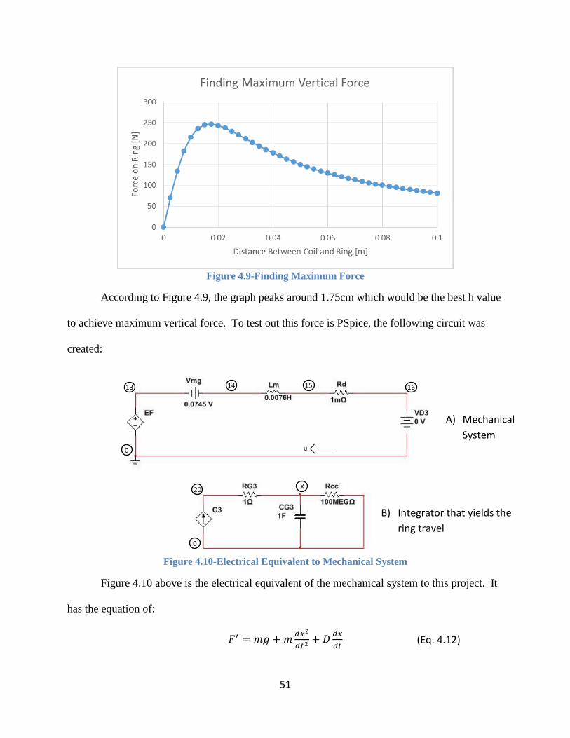
Figure 4.9-Finding Maximum Force
According to Figure 4.9, the graph peaks around 1.75cm which would be the best h value
to achieve maximum vertical force. To test out this force is PSpice, the following circuit was
created:
Figure 4.10-Electrical Equivalent to Mechanical System
Figure 4.10 above is the electrical equivalent of the mechanical system to this project. It
has the equation of:
13 14 15 16
0
0
20 X
A) Mechanical
System
B) Integrator that yields the
ring travel
u
52
(Eq. 4.14)
(Eq. 4.13)
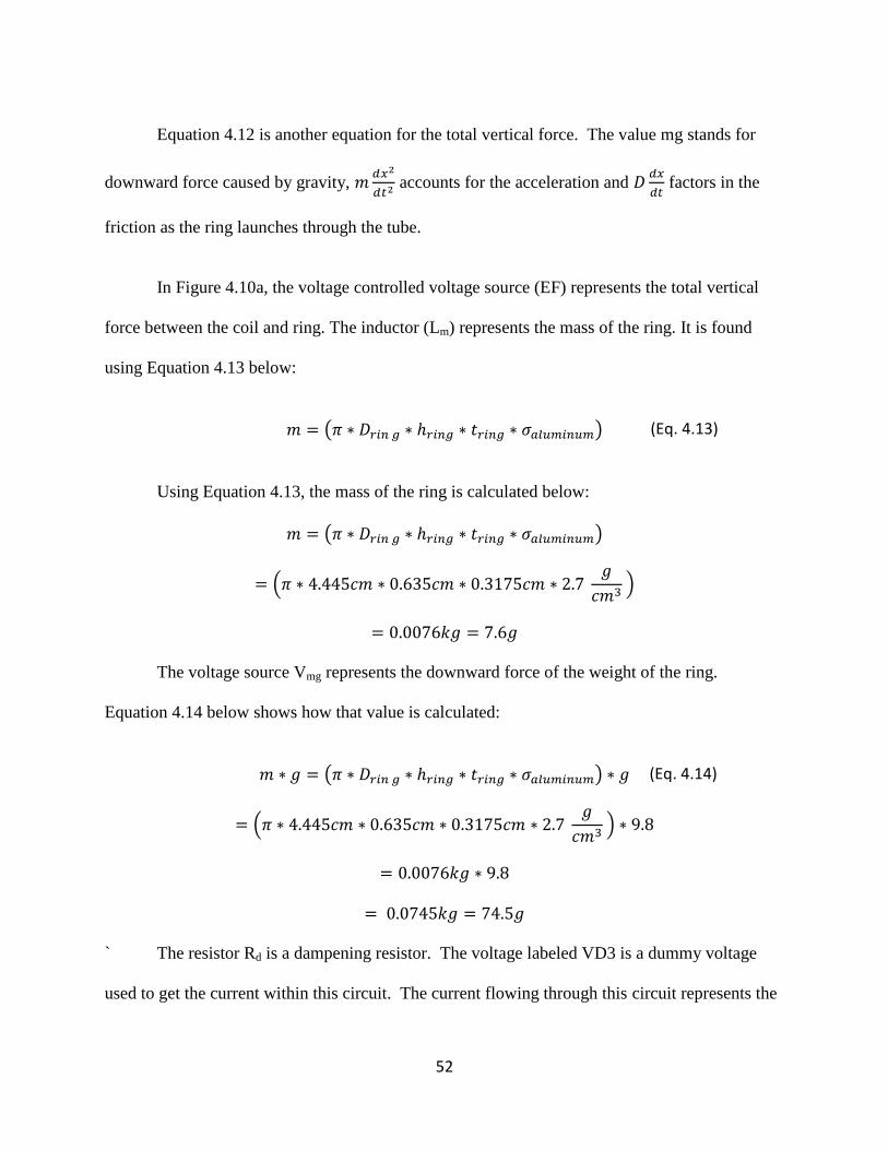
Equation 4.12 is another equation for the total vertical force. The value mg stands for
downward force caused by gravity,
accounts for the acceleration and
factors in the
friction as the ring launches through the tube.
In Figure 4.10a, the voltage controlled voltage source (EF) represents the total vertical
force between the coil and ring. The inductor (Lm) represents the mass of the ring. It is found
using Equation 4.13 below:
( )
Using Equation 4.13, the mass of the ring is calculated below:
( )
(
)
The voltage source Vmg represents the downward force of the weight of the ring.
Equation 4.14 below shows how that value is calculated:
( )
(
)
` The resistor Rd is a dampening resistor. The voltage labeled VD3 is a dummy voltage
used to get the current within this circuit. The current flowing through this circuit represents the

53
Key 1.0V=1.0 m
velocity of the ring (u) as it is launched. Figure 4.10b is used to get the maximum height that the
ring reaches. The following is the PSpice code for the mechanical circuit:
Figure 4.11-Mechanical System Code
As seen in Figure 4.11, the component EF takes the value of Equation 10. The values for
δ and cos(α) were calculated using the optimum value of h which came out to be 1.75cm. The
rest of the code consists of the components in Figure 4.10. From the PSpice code above, the
following graphs for the velocity and height were obtained:
Figure 4.12-Velocity and Height of Ring vs Time
Figure 4.12A represents the velocity of the ring and Figure 4.12B represents the height
traveled by the ring. Once the ring is launched, it reaches a top speed of about 14 m/s. The
velocity then decreases linearly and eventually reaches 0 m/s. While the velocity is positive, that
signifies when the ring is traveling upward, which can be seen in the height graph. When the
A) Velocity of the
ring
B) Height traveled
by the ring
54
velocity falls to 0 m/s, that is when the ring is at its’ peak height of about 9.25 meters. When the
velocity goes negative, that signifies when the ring is traveling downward. This can also be seen
on the height graph.
All of these graphs represent the greatest force, velocity, and height that the ring can
achieve with a 500V source. Experimentations can also be taken with different source voltages.
Experimenting With the Source Voltage
As what was stated earlier, different source voltages would result in different values of
force, velocity and height. Using the same optimal position of the ring that was found earlier, the
same methods were performed to discover the currents and height for source voltages of 100V,
300V and 1000V.
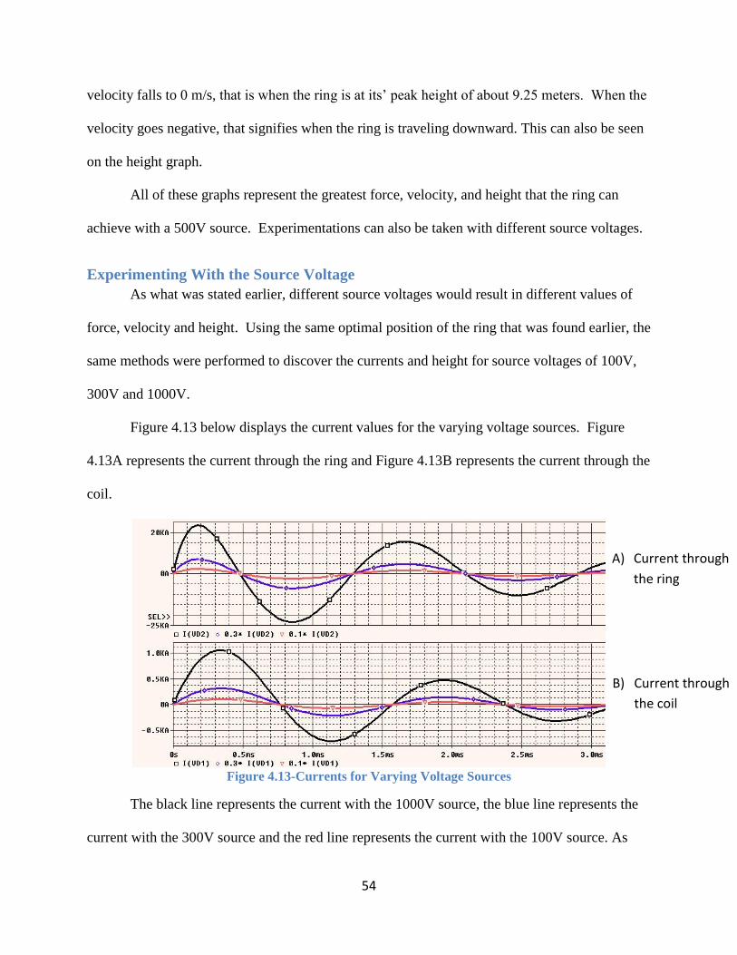
Figure 4.13 below displays the current values for the varying voltage sources. Figure
4.13A represents the current through the ring and Figure 4.13B represents the current through the
coil.
Figure 4.13-Currents for Varying Voltage Sources
The black line represents the current with the 1000V source, the blue line represents the
current with the 300V source and the red line represents the current with the 100V source. As
A) Current through
the ring
B) Current through
the coil
55
Key 1.0V=1.0 m
Key 10.0 mV=1.0 cm
shown, the 100V source has the highest current rating. Since the currents are proportional with
the voltage, the current with the 100V source would be
of the current with the 1000V source.
The same goes with the 300V source except that the current will be
the value of the current
with the 1000V source.
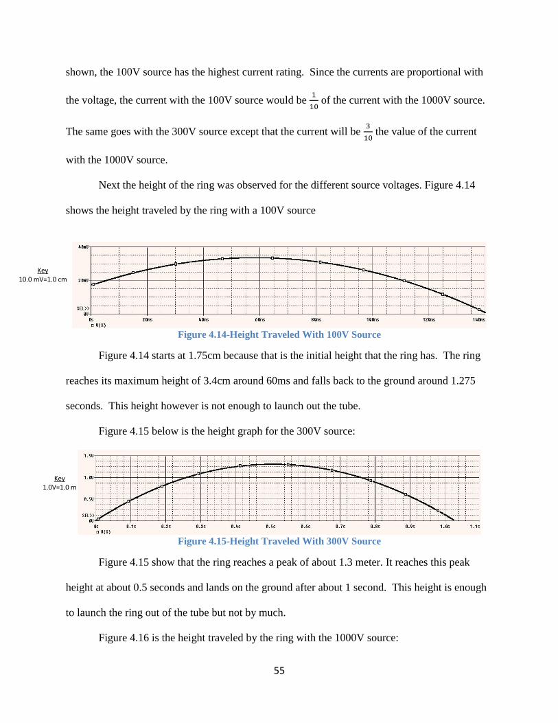
Next the height of the ring was observed for the different source voltages. Figure 4.14
shows the height traveled by the ring with a 100V source
Figure 4.14-Height Traveled With 100V Source
Figure 4.14 starts at 1.75cm because that is the initial height that the ring has. The ring
reaches its maximum height of 3.4cm around 60ms and falls back to the ground around 1.275
seconds. This height however is not enough to launch out the tube.
Figure 4.15 below is the height graph for the 300V source:
Figure 4.15-Height Traveled With 300V Source
Figure 4.15 show that the ring reaches a peak of about 1.3 meter. It reaches this peak
height at about 0.5 seconds and lands on the ground after about 1 second. This height is enough
to launch the ring out of the tube but not by much.
Figure 4.16 is the height traveled by the ring with the 1000V source:

56
Key 1.0V=1.0 m
Figure 4.16-Height Traveled With 1000V Source
As shown in Figure 4.16, at around 4.5 seconds, the ring reaches a maximum height of
about 110 meters and falls back to the ground after about 9.5 seconds.
Below is a clearer representation of the relation between source voltage and height
traveled:
Figure 4.17-Height Traveled with Varying Voltage Sources
Figure 4.17 above illustrates that the height traveled depends exponentially by the source
voltage.
57
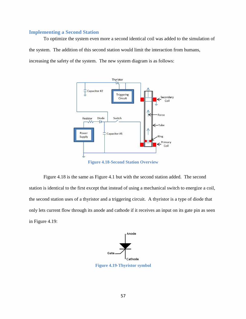
Implementing a Second Station
To optimize the system even more a second identical coil was added to the simulation of
the system. The addition of this second station would limit the interaction from humans,
increasing the safety of the system. The new system diagram is as follows:
Figure 4.18-Second Station Overview
Figure 4.18 is the same as Figure 4.1 but with the second station added. The second
station is identical to the first except that instead of using a mechanical switch to energize a coil,
the second station uses of a thyristor and a triggering circuit. A thyristor is a type of diode that
only lets current flow through its anode and cathode if it receives an input on its gate pin as seen
in Figure 4.19:
Figure 4.19-Thyristor symbol
58
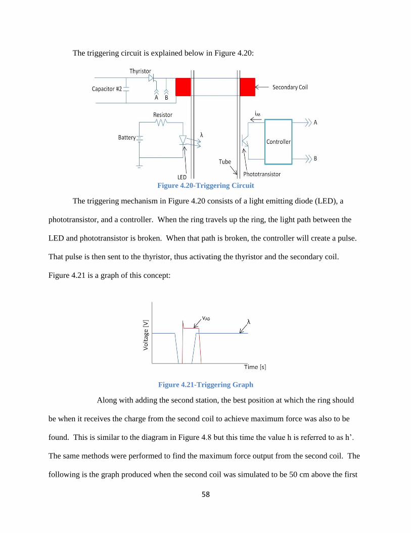
The triggering circuit is explained below in Figure 4.20:
Figure 4.20-Triggering Circuit
The triggering mechanism in Figure 4.20 consists of a light emitting diode (LED), a
phototransistor, and a controller. When the ring travels up the ring, the light path between the
LED and phototransistor is broken. When that path is broken, the controller will create a pulse.
That pulse is then sent to the thyristor, thus activating the thyristor and the secondary coil.
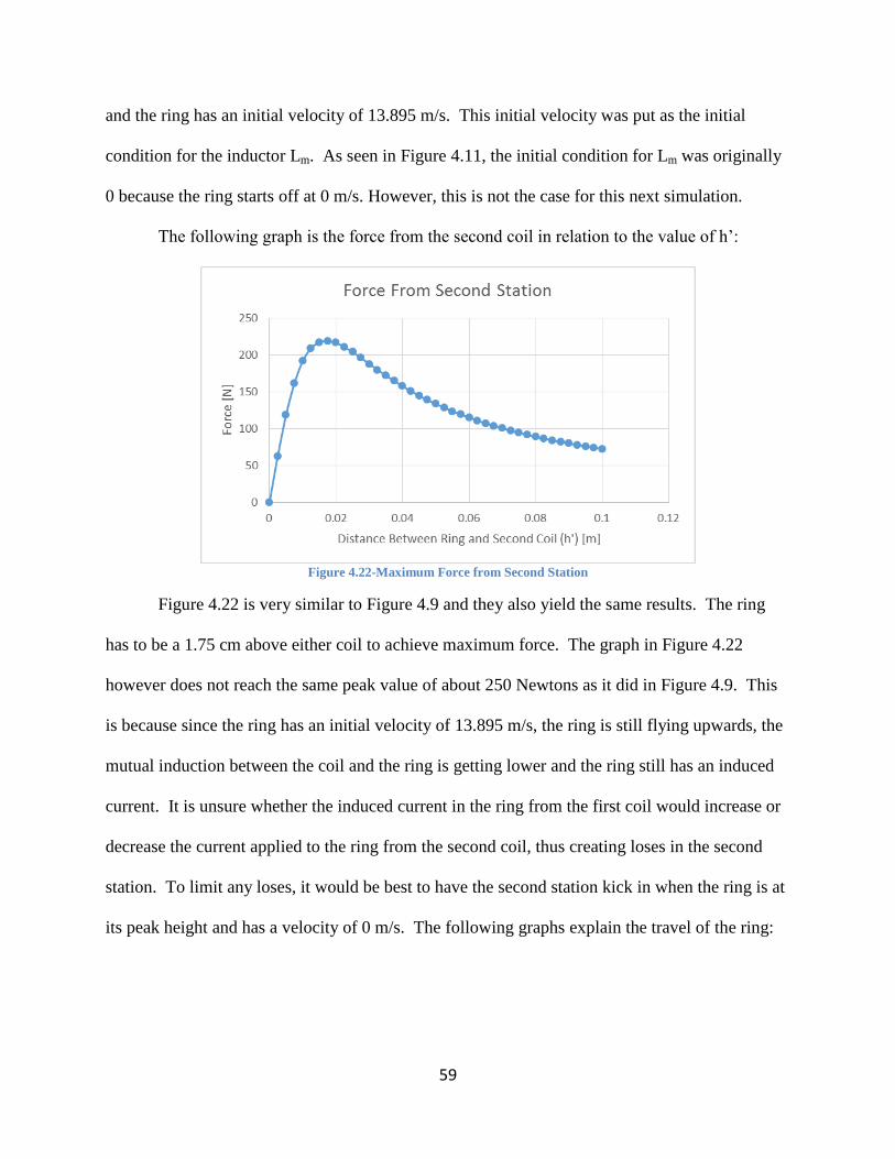
Figure 4.21 is a graph of this concept:
Figure 4.21-Triggering Graph
Along with adding the second station, the best position at which the ring should
be when it receives the charge from the second coil to achieve maximum force was also to be
found. This is similar to the diagram in Figure 4.8 but this time the value h is referred to as h’.
The same methods were performed to find the maximum force output from the second coil. The
following is the graph produced when the second coil was simulated to be 50 cm above the first
59
and the ring has an initial velocity of 13.895 m/s. This initial velocity was put as the initial
condition for the inductor Lm. As seen in Figure 4.11, the initial condition for Lm was originally
0 because the ring starts off at 0 m/s. However, this is not the case for this next simulation.
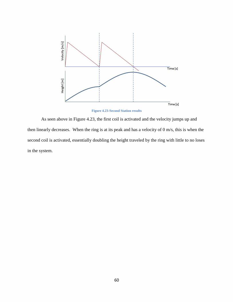
The following graph is the force from the second coil in relation to the value of h’:
Figure 4.22-Maximum Force from Second Station
Figure 4.22 is very similar to Figure 4.9 and they also yield the same results. The ring
has to be a 1.75 cm above either coil to achieve maximum force. The graph in Figure 4.22
however does not reach the same peak value of about 250 Newtons as it did in Figure 4.9. This
is because since the ring has an initial velocity of 13.895 m/s, the ring is still flying upwards, the
mutual induction between the coil and the ring is getting lower and the ring still has an induced
current. It is unsure whether the induced current in the ring from the first coil would increase or
decrease the current applied to the ring from the second coil, thus creating loses in the second
station. To limit any loses, it would be best to have the second station kick in when the ring is at
its peak height and has a velocity of 0 m/s. The following graphs explain the travel of the ring:
60
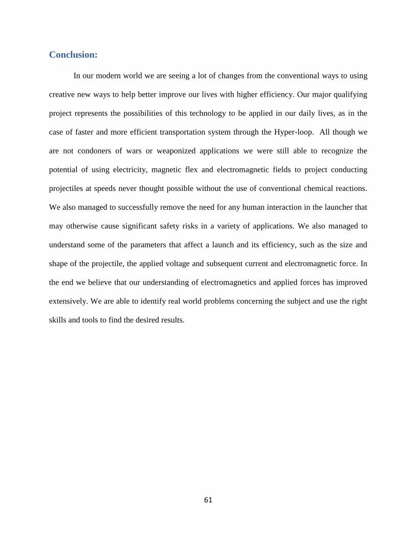
Figure 4.23-Second Station results
As seen above in Figure 4.23, the first coil is activated and the velocity jumps up and
then linearly decreases. When the ring is at its peak and has a velocity of 0 m/s, this is when the
second coil is activated, essentially doubling the height traveled by the ring with little to no loses
in the system.
61
Conclusion:
In our modern world we are seeing a lot of changes from the conventional ways to using
creative new ways to help better improve our lives with higher efficiency. Our major qualifying
project represents the possibilities of this technology to be applied in our daily lives, as in the
case of faster and more efficient transportation system through the Hyper-loop. All though we
are not condoners of wars or weaponized applications we were still able to recognize the
potential of using electricity, magnetic flex and electromagnetic fields to project conducting
projectiles at speeds never thought possible without the use of conventional chemical reactions.
We also managed to successfully remove the need for any human interaction in the launcher that
may otherwise cause significant safety risks in a variety of applications. We also managed to
understand some of the parameters that affect a launch and its efficiency, such as the size and
shape of the projectile, the applied voltage and subsequent current and electromagnetic force. In
the end we believe that our understanding of electromagnetics and applied forces has improved
extensively. We are able to identify real world problems concerning the subject and use the right
skills and tools to find the desired results.
62
Appendix A
The induction of the coil was found using the circuit in Figure X.5. Through this circuit,
the current resonates at 105 kHz and that corresponds to an induction value of 230µH. This was
proved in simulation by running AC analysis on the above circuit. Below in Figure X.A2 is the
simulation code:
Figure A1-AC Analysis code
The code in Figure A1 has an AC source with amplitude of 1V. The coil has the
inductance value of 230µH, the resistance of 100 Ω and a capacitor of 0.01µF. Running this
simulation yields the following graph:
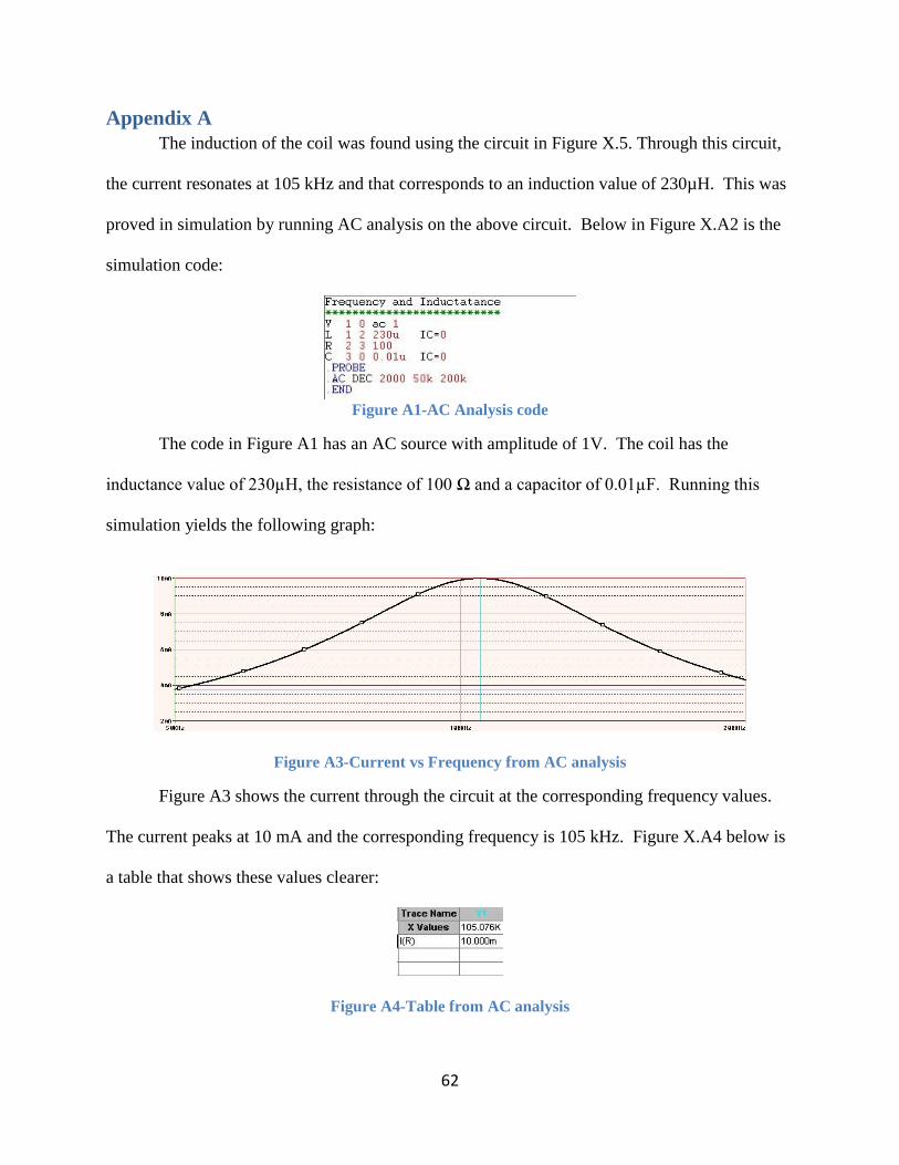
Figure A3-Current vs Frequency from AC analysis
Figure A3 shows the current through the circuit at the corresponding frequency values.
The current peaks at 10 mA and the corresponding frequency is 105 kHz. Figure X.A4 below is
a table that shows these values clearer:
Figure A4-Table from AC analysis

63
Appendix B - Calculations of Lyle’s Method

64
References
1. Grover, Frederick W. (1946). Inductance Calculations: Working Formulas and Tables.
New York: Van Nostrand-Reinhold