Electromagnetic Propagation (EPT1) Log Interpretation on the Computer

By Andy May2

1Mark of Schlumberger

2Senior Staff Geologist, Kerr McGee, Oklahoma City

Dielectric logging has been available commercially fromSchlumberger and other logging companies for over 10 years. Thesetools are very useful in evaluating formations drilled with oil-based mud, formations that contain fresh water, and in thin-beddedreservoirs. In particular, in wells drilled with oil-based mud,these tools can be invaluable when used to find the top of the oil-water transition zone. Dielectric tools are also used to correctfor the effect of invaded oil on density and induction logs.1.

Yet, interpreting dielectric logs continues to be very difficult. The mathematics that describe the tool's response are very complex. In addition, a battle over which of several complex interpretationmethods is best has been raging in the technical journals for overten years.

Unlike the more commonly used logging tools, it is difficult forthe practicing geoscientist and log analyst to get a "feel" for theEPT. The mathematics that describe the theory of microwave loggingare not the straightforward linear and logarithmic functions thatwe associate with density or electric logs. Instead, difficultfunctions of complex numbers describe dielectric log response. These functions fill dielectric logging papers with greek lettersand equations that only die-hard mathematicians could love.

The purpose of this paper is not to present anything new, but topresent a concise synthesis of dielectric log theory, and apractical, accurate, and up-to-date computer algorithm forinterpreting dielectric logs. The intent is to give the readerthat "feel" for the tool that is so important in interpreting alog. While researching this paper the author tried just aboutevery technique proposed for interpreting the dielectric logs, butonly one is presented here.

The "Modified CRIM" method, originally published by Dahlberg andFerence4, with a few original modifications, is the basis for theprogram presented in this paper. Essentially the same algorithm wasindependently developed at Schlumberger and published as the CTAmethod by Chardac2, Cheruvier and Suau3. The jury is still out onthe subject of the "correct" way to interpret the EPT, but thismethod leads the pack today.

Dielectric Logging Theory

EPT porosity is the quantity calculated using the toolmeasurements. This porosity(þept) is equivalent to the water-filledporosity in the near borehole region. This is the volume of waterin the flushed zone, which is equal to porosity(þ) times theflushed zone water saturation (Sxo). The tool works because therelative dielectric permittivity (î') of water is about 78 and therelative dielectric permittivity of oil, gas, and sedimentary rockis very low, normally less than 10.

A rock's complex dielectric permittivity describes the rock'selectrical properties. This is the quantity that the EPT toolattempts to measure. The complex dielectric permittivity isdefined as:

î* = î' - (å/þ)i ......................(1)

Where (þ) is the angular frequency (2ãþfrequency), (å) is theconductivity, (î') is the effective permittivity, and (i) is thesquare root of (-1). The equation shows that at low frequencies(like those used in induction logging) the imaginary part of (î*),the rock's conductivity, dominates the electrical properties of therock. Further, it shows that at very high frequencies the realpart of (î*), or the rock's effective permittivity, is dominant.

Equation (1) has one other property, when the rock's conductivityis very small compared to the frequency, the complex dielectricpermittivity is a real number and is easily evaluated. This istrue of a non-conductive rock matrix filled with fresh water andoil or gas. In these situations all the normal methods ofevaluating the EPT work very well. These methods include the TPOmethod9, the Complex Refractive Index Method (CRIM)9, and the Hanai-Bruggeman-Sen(HBS)7,8 method.

Early workers on the dielectric logging tool hoped that the veryhigh frequencies used by the tool would allow the computation ofwater saturation independently of Rw. This is essentially theassumption made when using the TPO equation. In practice, ignoringRw can only be done when Rw is greater than about 0.2 ohms at 75þF. In this higher Rw range any of the equations cited above can beused to evaluate þept. When Rw is less than 0.2 either CRIM or themore general HBS equations must be used.

Figure 1 shows the effect of salinity on þept. The center line isan assumed Sxo. The lower line is the computed Sxo if the waterhas a salinity of 60,000 PPM. The upper line is the computed Sxoat 200,000 PPM. The potential error is over 20 at 50% Sxo in thishypothetical case. The error is very small at low Sxo's, encouraging the use of the EPT in oil-based mud systems.

Two researchers7,8 have compared both the HBS þept and the CRIM þeptto laboratory measured water volumes, in various rock types andwith waters of varying salinities. These studies wereinconclusive, since one author determined that CRIM was a bettermethod7 and the other determined that the HBS method was superior8. But, the studies did show that the CRIM þept was an acceptableestimate of Sxo under ideal laboratory conditions. The programpresented in this issue uses a derivative of CRIM. The form of theequations used is very different from the equations presented inthe original CRIM paper9, and so the method used is often calledthe Complex Time Average (CTA) method. But, the two methods areequivalent, as demonstrated elsewhere3,4. The key equations, thatconnect the log readings used in the CTA method and the dielectricpermittivity values used in CRIM are:

î'/î0 = 0.09018 (Tpl2 - (Att/60.03)2)................(2)

î"/î0 = (å/þ)/î0 = Att þ Tpl/333.5..................(3)

Tpl is the log propagation time in nano-seconds/meter, Att is theplane-wave corrected log attenuation in dB/meter. We have dividedthe two parts of the complex dielectric permittivity (î' and î") bythe permittivity of a vacuum î0 (8.854 x 10-12) to turn them intorelative dielectric permittivities. This makes the numbers easierto handle. Typically when one sees a value of dielectricpermittivity quoted for a substance (eg. 79 for water) the numberis a relative dielectric permittivity.

The CTA equations have two common variables, salinity and þept. Thesolution process used in the computer program solves for these twovalues using the EPT log measured Tpl and Att. The equations are:

þept = (Tpl - Tpm + þt(Tpm-Tphc)) / (Tpw-Tphc).....(4)

þept = Att/Attw....................................(5)

Figure 2 shows how Tpw (the Propagation Time of water innanosec/m), Attw (the Attenuation of water in Db/m), and salinityare related. As salinity (the values posted next to the squares onthe line) increases, the values for Tpw and Attw also increase. Each salinity predicts a unique pair of Attw and Tpw values andvice-versa. Thus after equation 4 is used to compute þept, thisvalue can be used to compute Attw with equation 5. The new value ofAttw predicts a new salinity. The new salinity is used to reenterequation 4 with a revised Tpw, to compute a new þept. This cyclecontinues until the values of salinity and þept stabilize. Iterating in this fashion will solve the two equations for bothsalinity and þept, if the data is accurate.

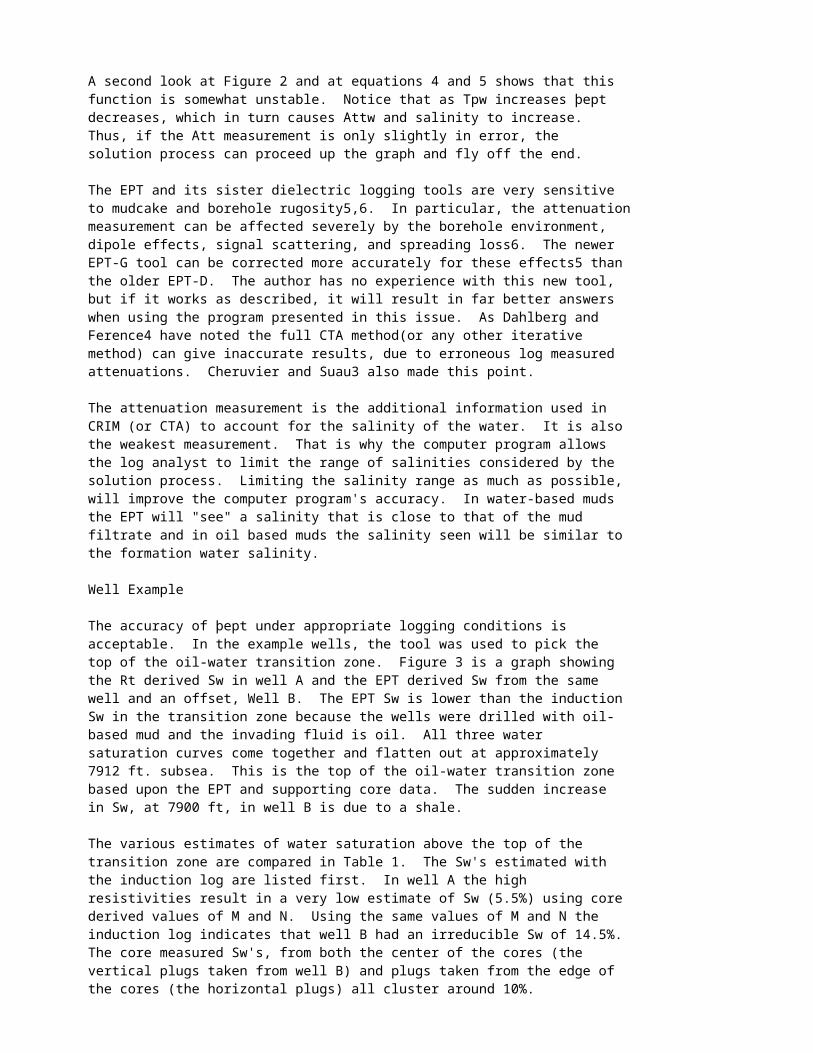
A second look at Figure 2 and at equations 4 and 5 shows that thisfunction is somewhat unstable. Notice that as Tpw increases þeptdecreases, which in turn causes Attw and salinity to increase. Thus, if the Att measurement is only slightly in error, thesolution process can proceed up the graph and fly off the end.

The EPT and its sister dielectric logging tools are very sensitiveto mudcake and borehole rugosity5,6. In particular, the attenuationmeasurement can be affected severely by the borehole environment, dipole effects, signal scattering, and spreading loss6. The newerEPT-G tool can be corrected more accurately for these effects5 thanthe older EPT-D. The author has no experience with this new tool,but if it works as described, it will result in far better answerswhen using the program presented in this issue. As Dahlberg andFerence4 have noted the full CTA method(or any other iterativemethod) can give inaccurate results, due to erroneous log measuredattenuations. Cheruvier and Suau3 also made this point.

The attenuation measurement is the additional information used inCRIM (or CTA) to account for the salinity of the water. It is alsothe weakest measurement. That is why the computer program allowsthe log analyst to limit the range of salinities considered by thesolution process. Limiting the salinity range as much as possible,will improve the computer program's accuracy. In water-based mudsthe EPT will "see" a salinity that is close to that of the mudfiltrate and in oil based muds the salinity seen will be similar tothe formation water salinity.

Well Example

The accuracy of þept under appropriate logging conditions isacceptable. In the example wells, the tool was used to pick thetop of the oil-water transition zone. Figure 3 is a graph showingthe Rt derived Sw in well A and the EPT derived Sw from the samewell and an offset, Well B. The EPT Sw is lower than the inductionSw in the transition zone because the wells were drilled with oil-based mud and the invading fluid is oil. All three watersaturation curves come together and flatten out at approximately7912 ft. subsea. This is the top of the oil-water transition zonebased upon the EPT and supporting core data. The sudden increasein Sw, at 7900 ft, in well B is due to a shale.

The various estimates of water saturation above the top of thetransition zone are compared in Table 1. The Sw's estimated withthe induction log are listed first. In well A the highresistivities result in a very low estimate of Sw (5.5%) using corederived values of M and N. Using the same values of M and N theinduction log indicates that well B had an irreducible Sw of 14.5%. The core measured Sw's, from both the center of the cores (thevertical plugs taken from well B) and plugs taken from the edge ofthe cores (the horizontal plugs) all cluster around 10%.

One would ordinarily assume that the EPT estimates of Sw, above thetransition zone, are valid. Above the top of the oil-watertransition zone, the invading oil from the mud will not move theconnate water since the rock is at irreducible water saturation.Yet, compared to the Rt and core measured Sw's, the EPT values arelow.

Oil and gas have very low relative dielectric permittivities andlow propagation times (Tpl). The Tpl of the oil-based mud

filtrate, used to drill the example wells, is 4.7 ns/m. This cancause the EPT signal to "short circuit" through the mud that liesbetween the EPT pad and the borehole wall. The example wells havea very thin mudcake, less than one-eighth inch thick, typical ofwells drilled with oil-based mud, but still some "short-circuiting"occurs. This has caused the EPT Sw's in the example wells to betoo low, the effect is discussed in the literature5,9. In theexample wells, and in other area wells, the effect is a constantoffset that can be corrected by comparing the EPT Sw's to coredata.

The Program

The main program asks the user for the necessary constants, for theinput file name and for the output file name. If the output filename is "*" then the program sends the output to the screen.

The first constant requested is the Tpl of the matrix(TPM). Thisvalue can be measured from cores or obtained from a chartbook. Toprocess the supplied test data, use the sandstone value of 7.2ns/m. The second and third constants requested are the minimum andmaximum salinity values. These values constrain the solutionprocess. The function CTA will attempt to solve for salinity andþept, these minimum and maximum values will keep the solutionprocess from "going wild," as discussed above, when it encountersincorrect attenuation values.

Next the main routine asks for the formation temperature in degreesFahrenheit. Using the temperature, an array is initialized by thefunction LOSS that is used by the function CTA to compute salinityfrom water attenuation. Finally the hydrocarbon propagation timewill be requested. This value can be input directly or as ahydrocarbon density1 in g/cc.

After obtaining the input constants from the user, the main routinegoes into a loop. The input data are read, one depth at a time,using format 1000. The variables read are described in thecomments preceding the read statement. All of the variables are

not used by the program, some are supplied only for the reader'sinformation.

Immediately after reading each line (or depth) of data, the valueof KPPMIN (the minimum salinity) is reset to the input value KPPM. This is done because the function CTA returns the computed salinityin KPPMIN each time it is called.

After calling CTA to do the computations, the main program callseither PRTVAL to write the results to a file, or SCRVAL to writethe results to the screen. The variable PAGESZ controls theplacement of the page headings. To remove the page headingsaltogether, enter a PAGESZ of zero.

The Calculations

The calculations are performed with the function CTA. The functionreturns Sxo. KPPM, the computed salinity, is returned as thevariable KPPMIN. The work of the function is done in the DO loop. The function calls EPSWA in each loop to compute the values of TPW(the water propagation time) and ATTW (the water attenuation)associated with the current estimate of KPPM. The first estimateof KPPM tried is KPPMIN, the minimum salinity expected by the user.

EPSWA is a function modified from one published by Dahlberg andFerence4. It is used here with their permission. This functionuses a complex, but accurate, method to compute TPW and ATTW forwater of a particular salinity and temperature.

Next, TPLMET is called to compute Sxo from the TPL and TPWsupplied. This estimate of Sxo is then used to compute ATTW withthe second of the CTA equations. The function SALIN converts theATTW to salinity using the table previously built by the functionLOSS.

The computed salinity (SAL) is carefully constrained to the userdefined limits with the next three statements. Convergence isachieved when the current estimate of salinity is within 10% of theprevious estimate or when the current estimate of Sxo is withinone-half of one percent of the previous estimate.

The program has been tested with the wells used as examples in thispaper and with many other wells drilled with both oil-based andwater-based muds. When properly used the program gives very goodresults. The key to successful use is determining KPPMAX andKPPMIN. Generally, set the range closely around the salinity ofthe mud filtrate when processing wells drilled with water-based

muds. Set the range closely around the formation water salinitywhen processing wells drilled with oil.

The best salinity range to use can be more accurately set byrunning trials on a selected subset of the data. The EPTattenuation measurement is the reason that the program seldomconverges and the reason why the salinity range is required. Ifthe attenuation measurement is accurate the program will convergeat the proper salinity, if it is off the program will not converge. If the program does not converge, the higher estimated salinity(KPPMAX) will probably be the value used. But the minimum valuemay be used in zones of high Sw. The attenuation measurement ismost accurate when the borehole walls are smooth, the mudcake isthin, and the volume of water (þept) is greater than 0.1. Underthese conditions, the user should see several intervals where theprogram reaches convergence on a salinity. These values can beused to select an appropriate range for KPPMIN and KPPMAX.

References

1. Boyeldieu, C., Coblentz, A., Pelissier-Combescure, J., "Formation Evaluation in Oil Base Mud Wells," SPWLA Symposium, June, 1984, paper BB.

2. Chardac, J. L. M., "EPT Applications in the Middle East,", SPE 13737, SPE 1985 Middle East Oil Technical Conterence, March, 1985.

3. Cheruvier, E. and Suau, J., "Applications of Microwave Dielectric Measurements in Various Logging Environments," paper MMM, 1986 SPWLA Symposium Transactions.

4. Dahlberg, K. E., and Ference, M. V., "A Quantitative Test of the Electromagnetic Propagation Log (EPT) for Residual Oil Determination," SPWLA Symposium Transactions, June, 1984.

5. Freedman, R. and Grove, G. P., "Interpretation of EPT-G Logs in the Presence of Mudcakes," SPE 18116, Presented at the 1988 SPE Conference, Oct., 1988.

6. Gilmore, R. J., Clark, B., Best, D., "Enhanced Saturation Determination Using The EPT-G Endfire Antenna Array," Paper K, 1987 SPWLA Symposium.

7. Shen, L. C., Savre, W. C., Price, J. M., Athavale, K., "Dielectric Properties of Reservoir Rocks at Ultra-High Frequencies," Geophysics, Vol. 50, No. 4, April, 1985, p. 692- 704.

8. Sherman, Michael M., "The Calculation of Porosity from Dielectric Constant Measurements: A Study using Laboratory Data," The Log Analyst, Jan.-Feb., 1986, p. 15-24.

9. Wharton, R. P., Hazen, G. A., Rau, R. N., and Best, D. L., "Electromagnetic Propagation Logging: Advances in Technique and Interpretation," SPE 9267, Presented at the 1980 SPE Conference, Sept., 1980.

ÉÍÍÍÍÍÍÍÍÍÍÍÍÍÍÍÍÍÍÍÍÍÍÍÍÍÍÍÍÍÍÍÍÍÍÍÍÍÍÍÍÍÍÍÍÍÍÍÍÍÍÍÍÍÍÍÍÍÍÍÍÍÍ» º Table 1 º º Comparison of Sw Estimates, Above Transition Zone º ÇÄÄÄÄÄÄÄÄÄÄÄÄÄÄÄÄÄÄÄÄÄÄÄÄÄÄÄÄÄÄÄÄÄÄÄÄÄÄÄÄÄÄÄÄÄÄÄÄÄÄÄÄÄÄÄÄÄÄÄÄÄĶ º Well Rt Sw EPT Core Core º º CTA Sw Vert. Sw Horiz. Swº ÇÄÄÄÄÄÄÄÄÄÄÄÄÄÄÄÄÄÄÄÄÄÄÄÄÄÄÄÄÄÄÄÄÄÄÄÄÄÄÄÄÄÄÄÄÄÄÄÄÄÄÄÄÄÄÄÄÄÄÄÄÄĶ º Well A 5.5 4.7 -- 8.3 º º Well B 14.5 6.1 10.4 12.5 º ÈÍÍÍÍÍÍÍÍÍÍÍÍÍÍÍÍÍÍÍÍÍÍÍÍÍÍÍÍÍÍÍÍÍÍÍÍÍÍÍÍÍÍÍÍÍÍÍÍÍÍÍÍÍÍÍÍÍÍÍÍÍͼ

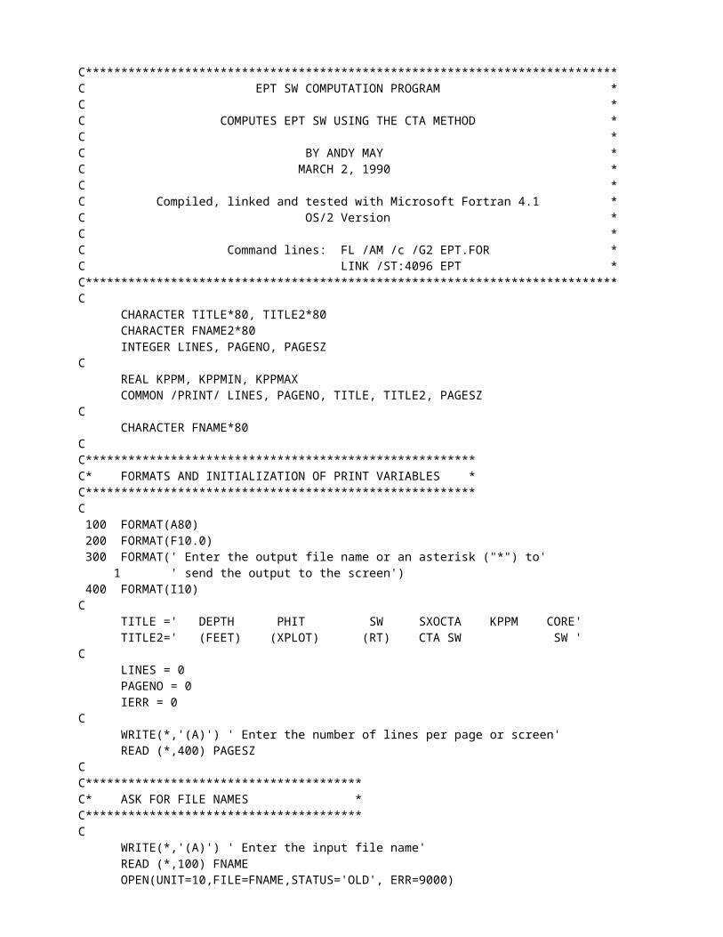
C***************************************************************************C EPT SW COMPUTATION PROGRAM *C *C COMPUTES EPT SW USING THE CTA METHOD *C *C BY ANDY MAY *C MARCH 2, 1990 *C *C Compiled, linked and tested with Microsoft Fortran 4.1 *C OS/2 Version *C *C Command lines: FL /AM /c /G2 EPT.FOR *C LINK /ST:4096 EPT *C***************************************************************************C CHARACTER TITLE*80, TITLE2*80 CHARACTER FNAME2*80 INTEGER LINES, PAGENO, PAGESZC REAL KPPM, KPPMIN, KPPMAX COMMON /PRINT/ LINES, PAGENO, TITLE, TITLE2, PAGESZC CHARACTER FNAME*80CC*******************************************************C* FORMATS AND INITIALIZATION OF PRINT VARIABLES *C*******************************************************C 100 FORMAT(A80) 200 FORMAT(F10.0) 300 FORMAT(' Enter the output file name or an asterisk ("*") to' 1 ' send the output to the screen') 400 FORMAT(I10)C TITLE =' DEPTH PHIT SW SXOCTA KPPM CORE' TITLE2=' (FEET) (XPLOT) (RT) CTA SW SW 'C LINES = 0 PAGENO = 0 IERR = 0C WRITE(*,'(A)') ' Enter the number of lines per page or screen' READ (*,400) PAGESZCC***************************************C* ASK FOR FILE NAMES *C***************************************C WRITE(*,'(A)') ' Enter the input file name' READ (*,100) FNAME OPEN(UNIT=10,FILE=FNAME,STATUS='OLD', ERR=9000)C WRITE(*,300) READ (*,100) FNAME2 IF (FNAME2(1:1) .NE. '*') 1 OPEN(UNIT=20, FILE=FNAME2, STATUS='NEW', ERR=9000)CC***************************************C* PICK UP CONSTANTS FROM SCREEN *C***************************************C

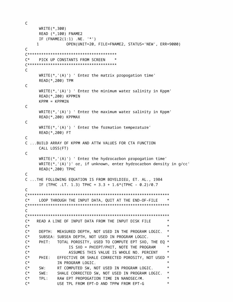
WRITE(*,'(A)') ' Enter the matrix propogation time' READ(*,200) TPMC WRITE(*,'(A)') ' Enter the minimum water salinity in Kppm' READ(*,200) KPPMIN KPPM = KPPMINC WRITE(*,'(A)') ' Enter the maximum water salinity in Kppm' READ(*,200) KPPMAXC WRITE(*,'(A)') ' Enter the formation temperature' READ(*,200) FTCC ...BUILD ARRAY OF KPPM AND ATTW VALUES FOR CTA FUNCTION CALL LOSS(FT)C WRITE(*,'(A)') ' Enter the hydrocarbon propogation time' WRITE(*,'(A)')' or, if unknown, enter hydrocarbon density in g/cc' READ(*,200) TPHCCC ...THE FOLLOWING EQUATION IS FROM BOYELDIEU, ET. AL., 1984 IF (TPHC .LT. 1.3) TPHC = 3.3 + 1.6*(TPHC - 0.2)/0.7CC**************************************************************C* LOOP THROUGH THE INPUT DATA, QUIT AT THE END-OF-FILE *C**************************************************************CC**************************************************************C* READ A LINE OF INPUT DATA FROM THE INPUT DISK FILE *C* *C* DEPTH: MEASURED DEPTH, NOT USED IN THE PROGRAM LOGIC. *C* SUBSEA: SUBSEA DEPTH, NOT USED IN PROGRAM LOGIC. *C* PHIT: TOTAL POROSITY, USED TO COMPUTE EPT SXO, THE EQ *C* IS SXO = PHIEPT/PHIT, NOTE THE PROGRAM *C* ASSUMES THIS VALUE IS WHOLE NO. PERCENT *C* PHIE: EFFECTIVE OR SHALE CORRECTED POROSITY, NOT USED *C* IN PROGRAM LOGIC. *C* SW: RT COMPUTED SW, NOT USED IN PROGRAM LOGIC. *C* SWE: SHALE CORRECTED SW, NOT USED IN PROGRAM LOGIC. *C* TPL: RAW EPT PROPOGATION TIME IN NANOSEC/M. *C* USE TPL FROM EPT-D AND TPPW FROM EPT-G *C* ATTEV: SPHERICAL SPREADING LOSS CORRECTED EPT *C* ATTENUATION. FOR EPT-G USE VALUE CALLED EAPW. *C* FOR EPT-D USE THE FOLLOWING EQUATION TO CORRECT *C* THE READING: *C* ATTEV = EATT - 45 - 1.3*TPL - 0.018*TPL*TPL *C* CORESW: CORE MEASURED SW, NOT USED IN PROGRAM LOGIC *C**************************************************************C 500 READ(10, 1000, END=3000, ERR=9000) 1 DEPTH, SUBSEA, PHIT, PHIE, SW, SWE, TPL, ATTEV, CORESW 1000 FORMAT(F8.0, F9.0, 5F7.0, F9.0, F7.0)CC...CTA METHOD KPPMIN = KPPM SXOCTA = CTA(TPM, TPHC, PHIT*0.01, TPL, ATTEV, KPPMIN, 1 KPPMAX, FT)*100.0CC...PRINT RESULTS IF (FNAME2(1:1) .NE. '*') THEN CALL PRTVAL(DEPTH, PHIT, SW, SXOCTA, KPPMIN, CORESW, IERR)

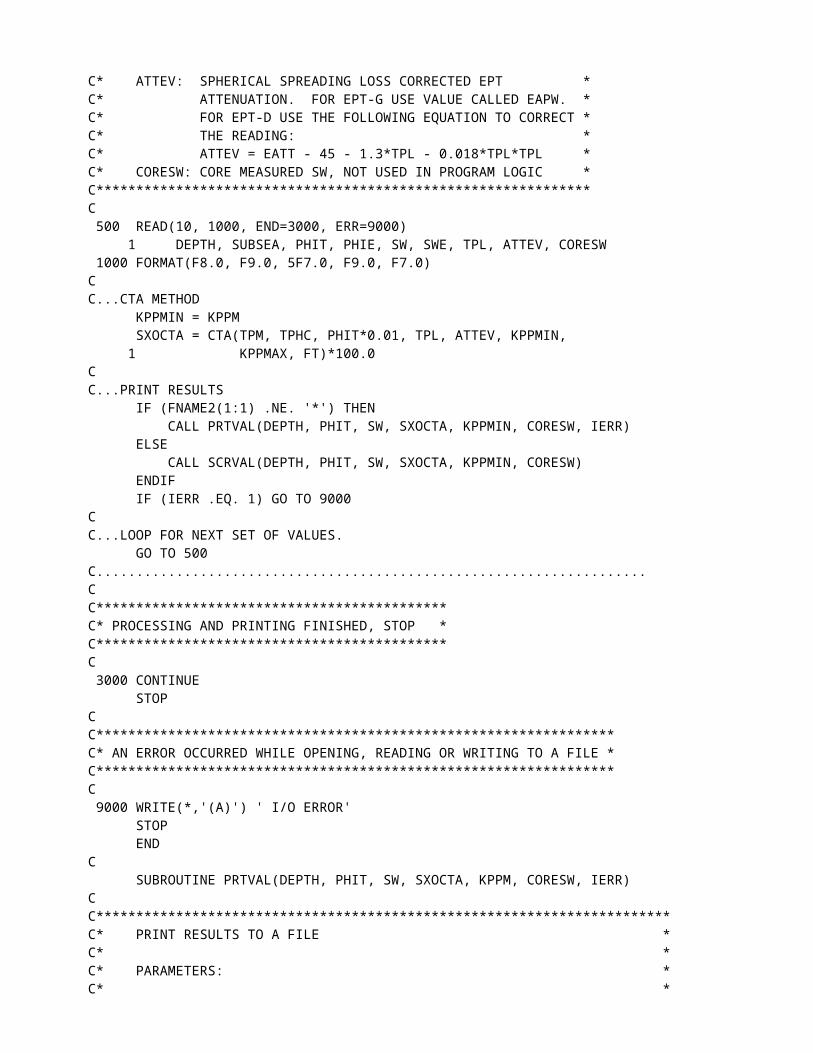
ELSE CALL SCRVAL(DEPTH, PHIT, SW, SXOCTA, KPPMIN, CORESW) ENDIF IF (IERR .EQ. 1) GO TO 9000CC...LOOP FOR NEXT SET OF VALUES. GO TO 500C.....................................................................CC********************************************C* PROCESSING AND PRINTING FINISHED, STOP *C********************************************C 3000 CONTINUE STOPCC*****************************************************************C* AN ERROR OCCURRED WHILE OPENING, READING OR WRITING TO A FILE *C*****************************************************************C 9000 WRITE(*,'(A)') ' I/O ERROR' STOP ENDC SUBROUTINE PRTVAL(DEPTH, PHIT, SW, SXOCTA, KPPM, CORESW, IERR)CC************************************************************************C* PRINT RESULTS TO A FILE *C* *C* PARAMETERS: *C* *C* DEPTH - MEASURED DEPTH OF VALUES *C* PHIT - THE TOTAL POROSITY OF THE ROCK (PERCENT) *C* SW - WATER SATURATION FROM RT *C* SXOCTA - SXO FROM THE CTA METHOD *C* KPPM - COMPUTED SALINITY *C* CORESW - CORE SW USING DEAN-STARKE METHOD *C* IERR - I/O ERROR FLAG: IF 0 OK; IF 1 ERROR *C* *C************************************************************************C REAL KPPM CHARACTER TITLE*80, TITLE2*80 INTEGER LINES, PAGENO, PAGESZC COMMON /PRINT/ LINES, PAGENO, TITLE, TITLE2, PAGESZC 1000 FORMAT(1X, 'PAGE ',I3) 2000 FORMAT(1X,A79) 3000 FORMAT(5F10.2, F8.2)CC...NEW PAGE? IF ( (LINES .EQ. PAGESZ .OR. LINES .EQ. 0) 1 .AND. PAGESZ .GT. 0) THENCC****************************C WRITE OUT TITLE LINES *C****************************C LINES = 0 PAGENO = PAGENO + 1

WRITE (20,1000, ERR=9000) PAGENOC WRITE(20, 2000, ERR=9000) TITLE, TITLE2 LINES = LINES + 3C ENDIFCC*************************C WRITE OUT RESULTS *C*************************C WRITE (20, 3000, ERR=9000) DEPTH, PHIT, SW, SXOCTA, KPPM, CORESW LINES = LINES + 1C RETURNC 9000 IERR = 1 RETURN ENDC SUBROUTINE SCRVAL(DEPTH, PHIT, SW, SXOCTA, KPPM, CORESW)CC************************************************************************C* PRINT RESULTS TO SCREEN *C* *C* PARAMETERS: *C* *C* DEPTH - MEASURED DEPTH OF VALUES *C* PHIT - THE TOTAL POROSITY OF THE ROCK (PERCENT) *C* SW - WATER SATURATION FROM RT *C* SXOCTA - SXO FROM THE CTA METHOD *C* KPPM - COMPUTED SALINITY *C* CORESW - CORE SW USING DEAN-STARKE METHOD *C* *C************************************************************************CC REAL KPPM CHARACTER TITLE*80, TITLE2*80, ENTER*4 INTEGER LINES, PAGENO, PAGESZC COMMON /PRINT/ LINES, PAGENO, TITLE, TITLE2, PAGESZC 1000 FORMAT(1X, 'PAGE ',I3) 2000 FORMAT(1X,A79) 3000 FORMAT(5F10.2, F8.2)CC...END OF SCREEN? IF (LINES .EQ. PAGESZ .OR. LINES .EQ. 0) THEN WRITE(*,'(A)') ' >>>> Press enter to continue. <<<<' READ(*,'(A)') ENTERCC****************************C WRITE OUT TITLE LINES *C****************************C LINES = 0 PAGENO = PAGENO + 1 WRITE (*,1000) PAGENOC WRITE(*, 2000) TITLE, TITLE2

LINES = LINES + 4C ENDIFCC*************************C WRITE OUT RESULTS *C*************************C WRITE (*, 3000) DEPTH, PHIT, SW, SXOCTA, KPPM, CORESW LINES = LINES + 1C RETURN ENDC FUNCTION CTA(TPM, TPHC, PHIT, TPL, ATTEV, KPPMIN, KPPMAX, FT)CC************************************************************************C* COMPUTE SXO FROM THE EPT USING THE CTA METHOD. *C* *C* ASSUMES THAT THE HARD PART OF THE ROCK IS LOSSLESS. ITERATES FOR *C* PHIEPT (EPT POROSITY), KPPM(WATER SALINITY). *C* *C* THE DIFFERENCE BETWEEN THIS FUNCTION AND CRIM IS THE METHOD OF *C* COMPUTING THE DIELECTRIC CONSTANT OF WATER AND THE FORM OF THE *C* EQUATIONS. CRIM USES WHARTON AND THIS FUNCTION USES DALHBERG AND *C* FERENCE. *C* *C* PARAMETERS: *C* *C* TPM - THE MATRIX TPL *C* TPHC - THE HYDROCARBON TPL *C* PHIT - THE TOTAL POROSITY OF THE ROCK AS A FRACTION *C* TPL - THE LOG MEASURED PROPOGATION TIME *C* ATTEV- THE LOSS CORRECTED EPT LOG MEASURED ATTENUATION *C* KPPMIN - ON INPUT, THE MINIMUM POSSIBLE WATER SALINITY. *C* ON OUTPUT, THE FUNCTION RETURNS THE BEST ESTIMATE *C* OF THE WATER SALINITY SEEN BY THE FUNCTION. *C* KPPMAX - THE MAXIMUM POSSIBLE WATER SALINITY IN THE NEAR *C* BOREHOLE REGION SEEN BY THE EPT LOG. FOR EXAMPLE, *C* IN THE CASE OF FRESH MUD AND SALINE FORMATION WATER *C* SET KPPMIN TO THE MUD SALINITY AND KPPMAX TO THE FORMATION *C* WATER SALINITY *C* FT - FORMATION TEMPERATURE IN DEGREES F. *C* *C* RETURNS THE COMPUTED VALUE OF SXO, AS A FRACTION *C* *C* FUNCTION BASED UPON THE METHOD OF SXO COMPUTATION DESCRIBED BY *C* CHERUVIER AND SUAU, 1986 SPWLA CONVENTION *C* *C************************************************************************C REAL KPPM, KPPMIN, KPPMAXCC...VALID POROSITY? CTA = 1.0 IF (PHIT .LE. 0.0) RETURNCC...SET INITIAL VALUES SXOPRV = 0.0 KPPM = KPPMINC

C************************************************************************C ITERATE FOR EPT POROSITY, SXO, AND KPPM A MAXIMUM OF 100 TIMES *C************************************************************************C DO 1000 I=1,100CC...COMPUTE TPW AND ATTW, USING DAHLBERG AND FERENCE CALL EPSWA(FT, KPPM, TPW, ATTW, EPW, EPPW)CC...SXO FROM EPT (SXOEPT) SXOEPT = TPLMET(TPM, PHIT, TPL, TPW, TPHC)C ATTW = ATTEV/(PHIT*SXOEPT)

C...CONVERT ATTW TO SALINITY (SAL) CALL SALIN(SAL, ATTW)CC...IF SAL IS -1 THE FUNCTION HAS GONE BEYOND THE END OF THE TABLEC...SO THIS STATEMENT WILL FORCE A SOLUTION AT THE LAST VALID POINT IF (SAL .LT. 0.0) SAL = KPPMAXCC...SOLUTIONS ARE DIFFICULT TO ACHIEVE WITH THIS FUNCTION.C...THE FOLLOWING FORCES THE ANSWER TO BE WITHIN REASONABLE BOUNDS IF (SAL .LT. KPPMIN) SAL = KPPMIN IF (SAL .GT. KPPMAX) SAL = KPPMAXCCC*************************************************************************C CHECK FOR CONVERGENCE. IF THE CURRENT ESTIMATE (SAL) IS *C WITHIN 10% OF THE PREVIOUS ESTIMATE (KPPM) OR THE CURRENT ESTIMATE *C OF SXO IS WITHIN 0.005 OF THE PREVIOUS ESTIMATE (SXOPRV) THEN RETURN *C KPPM AND CTA *C*************************************************************************C IF ( ABS(KPPM-SAL)/SAL .LT. 0.10 .OR. 1 ABS(SXOEPT-SXOPRV) .LT. 0.005) THEN KPPMIN = SAL CTA = SXOEPT RETURN ENDIFC SXOPRV = SXOEPT KPPM = SALC 1000 CONTINUEC................END OF ITERATION LOOPC KPPMIN = SAL CTA = SXOEPT RETURN ENDC FUNCTION TPLMET(TPM, PHIT, TPL, TPW, TPHC)CC************************************************************************C* COMPUTE SXO FROM THE EPT USING THE TPL METHOD. *C* *C* ASSUMES CONSTANT TPW, EG. TPW = TPL OF MUD FILTRATE, OR IF OBM *C* USED AND ABOVE TOP OF TRANSITION ZONE TPW = TPL OF FORMATION WATER*C* *C* PARAMETERS: *

C* *C* TPM - THE MATRIX TPL *C* PHIT - THE TOTAL POROSITY OF THE ROCK AS A FRACTION *C* TPL - THE LOG MEASURED PROPOGATION TIME *C* TPW - THE PROPOGATION TIME OF THE WATER *C* FT - FORMATION TEMPERATURE IN DEGREES F. *C* TPHC - THE HYDROCARBON PROPOGATION TIME *C* *C* RETURNS THE COMPUTED VALUE OF SXO, AS A FRACTION *C* *C* THIS METHOD IS RECOMMENDED BY DAHLBERG AND FERENCE, 1984. *C* *C************************************************************************C TPLMET = 1.0 IF (PHIT .LE. 0.0) RETURNC PHIEPT = (TPL - TPM + PHIT*(TPM - TPHC)) / (TPW - TPHC)C TPLMET = PHIEPT/PHIT IF (TPLMET .GT. 1.0) TPLMET = 1.0 IF (TPLMET .LT. 0.000001) TPLMET = 0.000001C RETURN ENDC SUBROUTINE EPSWA(FT, KPPM, TPW, ATTW, EFLP, EFLPP)CC************************************************************************C* COMPUTES TPW AND AW, THE PROPOGATION TIME AND ATTENUATION OF NACL *C* SOLUTIONS, AS FUNCTIONS OF TEMPERATURE (FAHRENHEIT) AND NACL *C* CONCENTRATION (KPPM). THE REAL AND IMAGINARY PARTS OF THE FLUID *C* DIELECTRIC PERMITTIVITY (EFLP AND EFLPP) ARE ALSO CALCULATED. *C* *C* THIS SUBROUTINE IS A SLIGHTLY MODIFIED VERSION OF ONE WRITTEN *C* BY DAHLBERG AND FERENCE. THE ORIGINAL WAS PUBLISHED AS *C* APPENDIX B, DAHLBERG AND FERENCE, 1984 *C* *C* USED WITH THE PERMISSION OF THE AUTHOR. *C************************************************************************C REAL KPPM DIMENSION TT(5), C(3), Z(3), BB(3,5) DATA BB /3.47, -6.65, 2.633, -59.21, 198.1, -64.8, 0.4551, 1 -0.2058, 0.005799, -9.346E-5, 7.368E-5, 6.741E-5, 2 -1.766E-6, 8.768E-7, -2.136E-7/CC************************************************************************C FLUID DIECTRIC PERMITTIVITY VIA COLE-COLE EQUATION *C OLHOEFT, "ELECTRICAL PROPERTIES OF ROCKS AND MINERALS, SHORT *C COURSE NOTES", GOLDEN, COLO., 1981. *C************************************************************************CC ...FREQUENCY OF THE TOOL IS 1.1 GIGAHERTZ FREQ = 1.1E9 OMEGA = 2.0*3.14159*FREQ T = (FT-32.0) * 0.555556 TKELV = T+273.0CC ...CONVERT NACL CONCENTRATION FROM KPPM TO MOLAR CMOLAR = 0.01722*KPPM

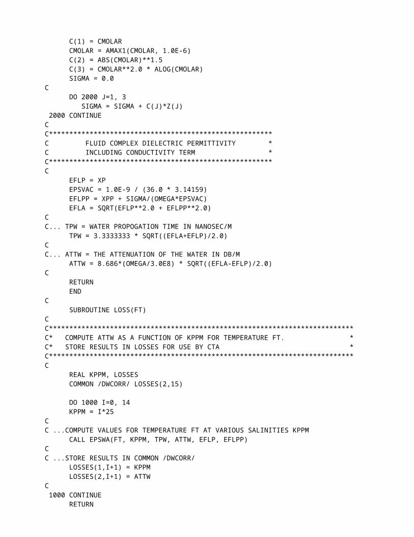
IF (KPPM .GT. 60.0) CMOLAR = 0.02*KPPM - 0.15 IF (KPPM .GT. 160.0) CMOLAR = 0.02238*KPPM - 0.53C TAU = 5.62E-15 * EXP(2182.0/TKELV) ALPHA = 0.0026 + 0.02676*CMOLAR - 0.00123*CMOLAR*CMOLAR 1 + 2.71E-5*CMOLAR**3.0 AEXP = 1.0 - ALPHA A = 1.0 + (OMEGA*TAU)**AEXP * COS(1.5708*AEXP) B = (OMEGA*TAU)**AEXP * SIN(1.5708*AEXP)C XINF = 4.2 + 0.2145*CMOLAR XST = 295.68 - 1.2283*TKELV + 2.094E-3 * TKELV*TKELV 1 - 1.41E-6*TKELV**3.0 XS = XST - 13.0*CMOLAR + 1.065*CMOLAR*CMOLAR 1 - 0.03006*CMOLAR**3.0C XP = XINF + (XS-XINF)*A / (A*A + B*B) XPP = (XS-XINF)*B / (A*A + B*B)CC ...FLUID CONDUCTIVITY (UCOK FORMULA FROM OLHOEFT, IBID.) TT(1) = 1.0 TT(2) = 1.0/T TT(3) = T TT(4) = T*T TT(5) = T*T*TC DO 1000 I=1, 3 Z(I) = 0.0 DO 1000 J=1, 5 Z(I) = Z(I) + BB(I,J)*TT(J) 1000 CONTINUEC C(1) = CMOLAR CMOLAR = AMAX1(CMOLAR, 1.0E-6) C(2) = ABS(CMOLAR)**1.5 C(3) = CMOLAR**2.0 * ALOG(CMOLAR) SIGMA = 0.0C DO 2000 J=1, 3 SIGMA = SIGMA + C(J)*Z(J) 2000 CONTINUECC*******************************************************C FLUID COMPLEX DIELECTRIC PERMITTIVITY *C INCLUDING CONDUCTIVITY TERM *C*******************************************************C EFLP = XP EPSVAC = 1.0E-9 / (36.0 * 3.14159) EFLPP = XPP + SIGMA/(OMEGA*EPSVAC) EFLA = SQRT(EFLP**2.0 + EFLPP**2.0)CC... TPW = WATER PROPOGATION TIME IN NANOSEC/M TPW = 3.3333333 * SQRT((EFLA+EFLP)/2.0)CC... ATTW = THE ATTENUATION OF THE WATER IN DB/M ATTW = 8.686*(OMEGA/3.0E8) * SQRT((EFLA-EFLP)/2.0)C RETURN ENDC

SUBROUTINE LOSS(FT)CC***************************************************************************C* COMPUTE ATTW AS A FUNCTION OF KPPM FOR TEMPERATURE FT. *C* STORE RESULTS IN LOSSES FOR USE BY CTA *C***************************************************************************C REAL KPPM, LOSSES COMMON /DWCORR/ LOSSES(2,15)

DO 1000 I=0, 14 KPPM = I*25CC ...COMPUTE VALUES FOR TEMPERATURE FT AT VARIOUS SALINITIES KPPM CALL EPSWA(FT, KPPM, TPW, ATTW, EFLP, EFLPP)CC ...STORE RESULTS IN COMMON /DWCORR/ LOSSES(1,I+1) = KPPM LOSSES(2,I+1) = ATTWC 1000 CONTINUE RETURN ENDC SUBROUTINE SALIN(KPPM, ATTW)CC***************************************************************************C* COMPUTE KPPM USING THE TABLE LOSSES AND THE SUPPLIED ATTW *C***************************************************************************C REAL KPPM, LOSSES COMMON /DWCORR/ LOSSES(2,15)

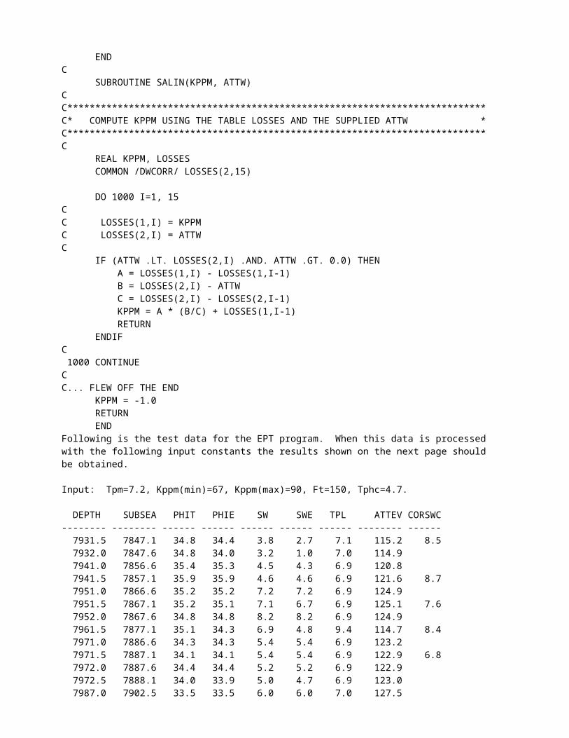
DO 1000 I=1, 15CC LOSSES(1,I) = KPPMC LOSSES(2,I) = ATTWC IF (ATTW .LT. LOSSES(2,I) .AND. ATTW .GT. 0.0) THEN A = LOSSES(1,I) - LOSSES(1,I-1) B = LOSSES(2,I) - ATTW C = LOSSES(2,I) - LOSSES(2,I-1) KPPM = A * (B/C) + LOSSES(1,I-1) RETURN ENDIFC 1000 CONTINUECC... FLEW OFF THE END KPPM = -1.0 RETURN ENDFollowing is the test data for the EPT program. When this data is processedwith the following input constants the results shown on the next page shouldbe obtained.

Input: Tpm=7.2, Kppm(min)=67, Kppm(max)=90, Ft=150, Tphc=4.7.

DEPTH SUBSEA PHIT PHIE SW SWE TPL ATTEV CORSWC-------- -------- ------ ------ ------ ------ ------ -------- ------ 7931.5 7847.1 34.8 34.4 3.8 2.7 7.1 115.2 8.5

7932.0 7847.6 34.8 34.0 3.2 1.0 7.0 114.9 7941.0 7856.6 35.4 35.3 4.5 4.3 6.9 120.8 7941.5 7857.1 35.9 35.9 4.6 4.6 6.9 121.6 8.7 7951.0 7866.6 35.2 35.2 7.2 7.2 6.9 124.9 7951.5 7867.1 35.2 35.1 7.1 6.7 6.9 125.1 7.6 7952.0 7867.6 34.8 34.8 8.2 8.2 6.9 124.9 7961.5 7877.1 35.1 34.3 6.9 4.8 9.4 114.7 8.4 7971.0 7886.6 34.3 34.3 5.4 5.4 6.9 123.2 7971.5 7887.1 34.1 34.1 5.4 5.4 6.9 122.9 6.8 7972.0 7887.6 34.4 34.4 5.2 5.2 6.9 122.9 7972.5 7888.1 34.0 33.9 5.0 4.7 6.9 123.0 7987.0 7902.5 33.5 33.5 6.0 6.0 7.0 127.5 7987.5 7903.0 33.6 33.6 6.1 6.1 7.0 127.5 7988.0 7903.5 34.1 34.1 6.0 6.0 7.0 127.5 7988.5 7904.0 34.0 32.7 3.9 1.0 7.1 127.5 7989.0 7904.5 33.9 33.6 5.3 4.5 7.1 127.6 8011.0 7926.5 33.4 33.4 16.7 16.7 7.6 135.6 8011.5 7927.0 34.0 33.4 15.2 13.7 7.6 136.1 12.5 8012.0 7927.5 34.4 34.4 16.7 16.6 7.6 136.4 8012.5 7928.0 33.9 33.6 16.3 15.5 7.7 136.7 8013.0 7928.5 33.6 32.6 14.8 12.4 7.7 137.2 8020.0 7935.5 33.0 32.9 20.3 20.0 7.6 141.0 8020.5 7936.0 33.2 33.2 20.9 20.9 7.6 143.5 8021.0 7936.5 33.3 33.3 21.2 21.2 7.6 144.4 8021.5 7937.0 33.6 33.6 21.1 20.9 7.6 146.0 8022.0 7937.5 33.4 32.8 20.0 18.4 7.6 145.2 15.1 8022.5 7938.0 33.8 33.3 20.6 19.4 7.7 145.1 8023.0 7938.5 34.2 33.6 20.4 19.0 7.7 144.2 8029.5 7945.0 34.8 34.8 29.7 29.7 7.9 147.8 8030.0 7945.5 34.9 34.4 29.2 28.3 7.9 148.5 8030.5 7946.0 34.8 34.8 32.1 32.1 8.0 149.6 8031.0 7946.5 35.2 35.2 33.3 33.3 8.0 150.8 8031.5 7947.0 35.4 35.4 34.8 34.8 8.0 152.6 23.4 8032.0 7947.5 35.5 35.5 36.6 36.6 8.0 154.6 8204.0 8122.0 31.4 31.4 100.0 100.0 11.4 404.0 8204.5 8122.5 30.9 30.9 100.0 100.0 11.4 397.8 8205.0 8123.0 30.6 30.6 100.0 100.0 11.4 378.0 25.8 8205.5 8123.5 30.3 29.9 100.0 100.0 11.7 374.7 8206.0 8124.0 29.4 29.4 100.0 100.0 11.8 370.1 8206.5 8124.5 29.1 29.1 100.0 100.0 12.0 382.3 8207.0 8125.0 29.5 29.5 100.0 100.0 12.4 387.9 8207.5 8125.5 31.1 30.6 100.0 100.0 13.1 393.0 8208.0 8126.0 32.8 31.9 100.0 100.0 14.1 388.9 8208.5 8126.5 33.1 31.1 99.8 99.7 14.8 398.4 8209.0 8127.0 31.9 29.1 100.0 100.0 15.1 402.2 40.2 8209.5 8127.5 31.2 31.2 100.0 100.0 14.6 410.8 8210.0 8128.0 32.9 32.9 100.0 100.0 14.3 423.6Following is the test case output. These results should be obtained when thetest data on the previous page is run.

PAGE 1 DEPTH PHIT SW SXOCTA KPPM CORE (FEET) (XPLOT) (RT) CTA SW SW 7931.5 34.80 3.80 5.38 90.00 8.50 7932.0 34.80 3.20 4.69 90.00 .00 7941.0 35.40 4.50 4.02 90.00 .00 7941.5 35.90 4.60 4.05 90.00 8.70 7951.0 35.20 7.20 4.01 90.00 .00 7951.5 35.20 7.10 4.01 90.00 7.60 7952.0 34.80 8.20 3.99 90.00 .00

7961.5 35.10 6.90 23.09 67.00 8.40 7971.0 34.30 5.40 3.96 90.00 .00 7971.5 34.10 5.40 3.94 90.00 6.80 7972.0 34.40 5.20 3.96 90.00 .00 7972.5 34.00 5.00 3.94 90.00 .00 7987.0 33.50 6.00 4.63 90.00 .00 7987.5 33.60 6.10 4.64 90.00 .00 7988.0 34.10 6.00 4.66 90.00 .00 7988.5 34.00 3.90 5.37 90.00 .00 7989.0 33.90 5.30 5.37 90.00 .00 8011.0 33.40 16.70 9.00 90.00 .00 8011.5 34.00 15.20 8.95 90.00 12.50 8012.0 34.40 16.70 8.91 90.00 .00 8012.5 33.90 16.30 9.67 90.00 .00 8013.0 33.60 14.80 9.71 90.00 .00 8020.0 33.00 20.30 9.03 90.00 .00 8020.5 33.20 20.90 9.02 90.00 .00 8021.0 33.30 21.20 9.01 90.00 .00 8021.5 33.60 21.10 8.98 90.00 .00 8022.0 33.40 20.00 9.00 90.00 15.10 8022.5 33.80 20.60 9.68 90.00 .00 8023.0 34.20 20.40 9.64 90.00 .00 8029.5 34.80 29.70 10.98 90.00 .00 8030.0 34.90 29.20 10.97 90.00 .00 8030.5 34.80 32.10 11.68 90.00 .00 8031.0 35.20 33.30 11.61 90.00 .00 8031.5 35.40 34.80 11.58 90.00 23.40 8032.0 35.50 36.60 11.57 90.00 .00 8204.0 31.40 100.00 38.64 90.00 .00 8204.5 30.90 100.00 39.16 90.00 .00 8205.0 30.60 100.00 39.49 90.00 25.80 8205.5 30.30 100.00 42.23 90.00 .00 8206.0 29.40 100.00 44.16 90.00 .00 8206.5 29.10 100.00 46.23 90.00 .00 8207.0 29.50 100.00 48.98 90.00 .00 8207.5 31.10 100.00 53.65 87.58 .00 8208.0 32.80 100.00 61.97 72.61 .00 8208.5 33.10 99.80 67.04 67.00 .00 8209.0 31.90 100.00 71.79 67.00 40.20 8209.5 31.20 100.00 69.03 73.04 .00 8210.0 32.90 100.00 63.40 67.00 .00