Embed Size (px)
Citation preview

School of Industrial and Information Engineering
Department of Chemistry, Materials and Chemical Engineering “G. Natta”
Master of Science in Materials Engineering and Nanotechnology
ELECTROCHEMICAL TESTING FOR PEDEFERRI
DIAGRAMS OF STAINLESS STEEL IN CHLORIDE
CONTAING ENIRONMENT
Supervisor: Prof. Fabio Maria BOLZONI
Co-supervisor: Ing. Andrea BRENNA
Dr. Arash AZIMI DASTGERDI
Filippo BEGNA 842090
Academic year 2015-2016

Table of Contents
INDEX OF FIGURES ................................................................................................................... 5
INDEX OF TABLES ..................................................................................................................... 9
ABSTRACT ITALIANO ............................................................................................................ 10
ABSTRACT .................................................................................................................................. 12
INTRODUCTION ...................................................................................................................... 13
1.1 BASICS OF CORROSION: THE ELECTROCHEMICAL MECHANISM 13
1.3.1 MECHANISM OF PIT INITIATION .................................................... 20
1.3.2 MECHANISM OF PIT PROPAGATION ............................................. 22
1.3.3 CREVICE CORROSION MECHANISM ................................................... 23
1.3.4 INITIATION OF CREVICE CORROSION ......................................... 23
1.3.5 PROPAGATION OF CREVICE CORROSION .................................. 24
.ELECTROCHEMICAL TEST METHODS FOR PITTING AND CREVICE
SUSCEPTIBILITY MEASUREMENTS .................................................................... 39
2.1 MEASUREMENTS WITH A POTENTIOSTAT ............................................ 40
2.1.1 CONTINOUS POTENTIODYNAMIC POLARIZATION ........................ 40
2.1.2 STEPWISE POTENTIODYNAMIC POLARIZATION ........................... 42
2.1.3 POTENTIOSTATIC POLARIZATION ...................................................... 42
2.1.4 COMPARISON BETWEEN POTENTIODYNAMIC AND
POTENTIOSTATIC POLARIZATION .................................................................... 45
2.2 MEASUREMENTS WITH A GALVANOSTAT ............................................. 45
2.2.1 GALVANOSTATIC POLARIZATION TEST ........................................... 46
2.2.2 STEPWISE GALVANIC POLARIZATION ................................................... 47
2.3 ELECTROCHEMICAL IMPEDANCE SPECTROSCOPY ............................. 47
2.4 SCRATCH METHOD .......................................................................................... 49
MATERIALS AND METHODS ................................................................................................ 50
3.1 MATERIAL ......................................................................................................... 50
3.2 SAMPLE PREPARATION ................................................................................ 50
3.3 APPARATUS AND TOOLS ............................................................................... 51
3.4 PRE-CONDITIONING TIME ........................................................................... 52
3.5 POTENTIODYNAMIC POLARIZATION TEST ........................................... 53
3.6 POTENTIOSTATIC POLARIZATION TEST ................................................ 54
RESULTS ..................................................................................................................................... 57

4.1. POTENTIODYNAMIC POLARIZATION TESTS ......................................... 57
4.1.1 EFFECT OF CHLORIDE CONCENTRATION .................................. 57
4.1.2 EFFECT OF SURFACE AREA ................................................................ 60
4.1.3 EFFECT OF SCAN RATE ..................................................................... 61
4.2 POTENTIOSTATIC POLARIZATION TESTS .............................................. 63
DISCUSSION ............................................................................................................................... 66
5.1 POTENTIODYNAMIC POLARISATION TEST ............................................... 66
5.1.1 EFFECT OF CHLORIDE CONCENTRATIONS ................................ 66
5.1.2 EFFECT OF SURFACE AREA ............................................................ 71
5.1.3 EFFECT OF POTENTIAL SCAN RATE ........................................... 73
5.2 POTENTIOSTATIC POLARISATION TESTS ............................................... 74
5.3 PEDEFERRI DIAGRAM .................................................................................... 76
CONCLUSIONS .......................................................................................................................... 79
BIBLIOGRAPHY ........................................................................................................................ 81

Index of FiguresIndex of Figures
4

Index of FiguresIndex of Figures
5
INDEX OF FIGURES
Figure 1.1 Schematic of the current circulation during a corrosion process, with the expression of
electroneutrality
Figure 1.2 Pourbaix diagram for a generic metallic material M which forms hydroxides
Figure 1.3 Evans diagram for a generic corrosion process: anodic (blue) and cathodic (red)
processes
Figure 1.4 Evans diagram for a generic anodic process of a passive metal
Figure 1.5 Schematic anodic polarization curve showing the pitting potential
Figure 1.6 Dependence of pitting potential in function of the chloride contents
Figure 1.7 Penetration mechanism of pitting corrosion
Figure 1.8 Film thinning mechanism of pitting
Figure 1.9 The film rupture mechanism of pitting
Figure 1.10 Schematic representation of the propagation stage of pitting
Figure 1.11 Schematic illustration of the initiation stage of crevice corrosion: (c) is an expanded
view of (a) and (b)
Figure 1.12 Schematic illustration of the propagation stage of crevice corrosion of iron
Figure 1.13 Schaeffler diagram
Figure 1.14 Pitting potential of Cr in the Fe-Cr alloys in0,1 M NaCl at 25°C
Figure 1.15 Effect of cold rolling on AISI 304 in 0,1 NaCl + 2x10⁻⁴ FeCl3
Figure 1.16 Potentiodynamic polarization curves for AISI 304 stainless steel samples submitted
to different surface finishing operations in 0,1 NaCl at room temperature; potential is taken respect
Ag/AgCl/KClsat reference electrode
Figure 1.17 Potentiodynamic curves for four different surface finishing of AISI 304 stainless steel
samples in 0,5 M NaCl, scan rate of 1 mV/h

Index of FiguresIndex of Figures
6
Figure 1.18 Effect of the temperature on the pitting potential of Alloy 600 in deaerated 0,282 M
NaCl solution
Figure 1.19 Effect of pH on pitting corrosion
Figure 1.20 Pedeferri’s diagram for the cathodic protection or prevention for the rebars in the
reinforce concrete
Figure 2.1 Plot of a potentiodynamic polarization
Figure 2.2 Dependence of breakdown potential on the scan rate
Figure 2.3 Current density vs Time depending on the polarization potential
Figure 2.4 The two ways to get critical chloride contents or pitting potential: potentiodynamic
(red) potentiostatic (blue)
Figure 2.5 Current density when pitting already initiate depending on the polarization potential:
Ea<Eb; plotted vs time
Figure 2.6 Potentiodynamic polarization curve (a) and potentiostatic polarization curve (b)
obtained for UNS S32404
Figure 2.7 The three regions of the chronopotentiometric curve: nucleation (1), propagation (2)
and protection (3)
Figure 2.8 Curve obtained with the stepwise galvanic polarization
Figure 3.1 Length and width of the AISI 304 sample used for tests
Figure 3.2 Apparatus for stepwise potentiodynamic and potentiostatic polarization tests
Figure 3.3 Apparatus for continuous potentiodynamic tests
Figure 3.4 The pre-conditioning time for AISI 304 at concentration of 3000 and 1000 ppm
chloride
Figure 4.1 Polarization curves of 100 ppm chloride, scan rate 600 mV/h, , 2 cm2, room temperature
Figure 4.2 Polarisation curves of 300 ppm chloride, scan rate 600 mV/h, 2 cm2, room temperature

Index of FiguresIndex of Figures
7
Figure 4.3 Anodic polarisation curves of 300 ppm chloride, scan rate 600 mV/h, 2 cm2, room
temperature
Figure 4.4 Polarisation curves of 3000 ppm chloride, scan rate 600 mV/h, 2 cm2, room temperature
Figure 4.5 Polarisation curves of 1000 ppm chloride, scan rate 600 mV/h, 10 cm2, room
temperature
Figure 4.6 Polarisation curves of 300 ppm chloride, scan rate 600 mV/h, 50 cm2, room
temperature
Figure 4.7 Curve of stepwise potentiodynamic polarization, 2 cm2, room temperature
Figure 4.8 Results for potentiostatic polarization at 0,42 V vs Ag/AgCl/KClsat
Figure 4.9 Results for potentiostatic polarization at 0,335 V vs Ag/AgCl/KClsat
Figure 5.1 Probability curve for all the concentration tested: a) 100 ppm, b) 300 ppm, c) 1000
ppm, d) 3000 ppm, e) 10000 ppm, f) 19000 ppm
Figure 5.2 Isoprobability curve for all the concentration tested ranging from 100 ppm to 19000
ppm
Figure 5.3 Isoprobability curve in semi-logarithm for all the concentration tested ranging from
100 ppm to 19000 ppm
Figure 5.4 Isoprobability curve for different surface area
Figure 5.5 Dependence of pitting potentials on the surface at fixed scan rate for samples of AISI
304 in 3,5% NaCl at 35°C
Figure 5.6 Pitting potential at 1000 ppm with three different potential scan rate
Figure 5.7 Pitting potential at 3000 ppm with three different potential scan rate
Figure 5.8 Pitting potential at 10000 ppm with three different potential scan rate
Figure 5.9 Percentage of corroded specimen in function of the chloride content for the
potentiostatic polarization at 0,335 V vs Ag/AgCl/KClsat
Figure 5.10 Percentage of corroded specimen in function of the chloride content for the
potentiostatic polarization at 0,335 V vs Ag/AgCl/KClsat

Index of FiguresIndex of Figures
8
Figure 5.11 Critical chloride concentration for three different polarization potentials
Figure 5.12 Comparison between all the tests conducted in this thesis and the previous ones
Figure 5.13 Final Pedeferri’s diagram, with all the areas higlined; used values corresponds to
experimental setup o 600 mV/h, 2 cm2 at room temperature

Index of TablesIndex of Figures
9
INDEX OF TABLES
Table 1.1 Approximated effect of the major alloying elements
Table 1.2 Effect of seawater flow rate on pitting of welded AISI 316 after 1257 days of exposure
Table 3.1 Chemical composition of AISI 304L used
Table 3.2 Procedure to prepare a 2 cm2
Table 3.3 Tests performed with different concentrations of chloride for different scan rates and
surface area
Table 3.4 Potentiostatic test specifications, conducted at room temperature
Table 4.1 Results for 1000 ppm, scan rate of 100 mV/h, 2 cm2, room temperature
Table 4.2 Results for 1000 ppm, scan rate of 10 mV/h, 2 cm2, room temperature
Table 4.3 Results for 3000 ppm, scan rate of 100 mV/h, 2 cm2, room temperature
Table 4.4 Results for 3000 ppm, scan rate of 10 mV/h, 2 cm2, room temperature
Table 4.5 Results for the stepwise potentiodynamic polarization, scan rate of 1 mV/h, surface area
of 2 cm2, room temperature
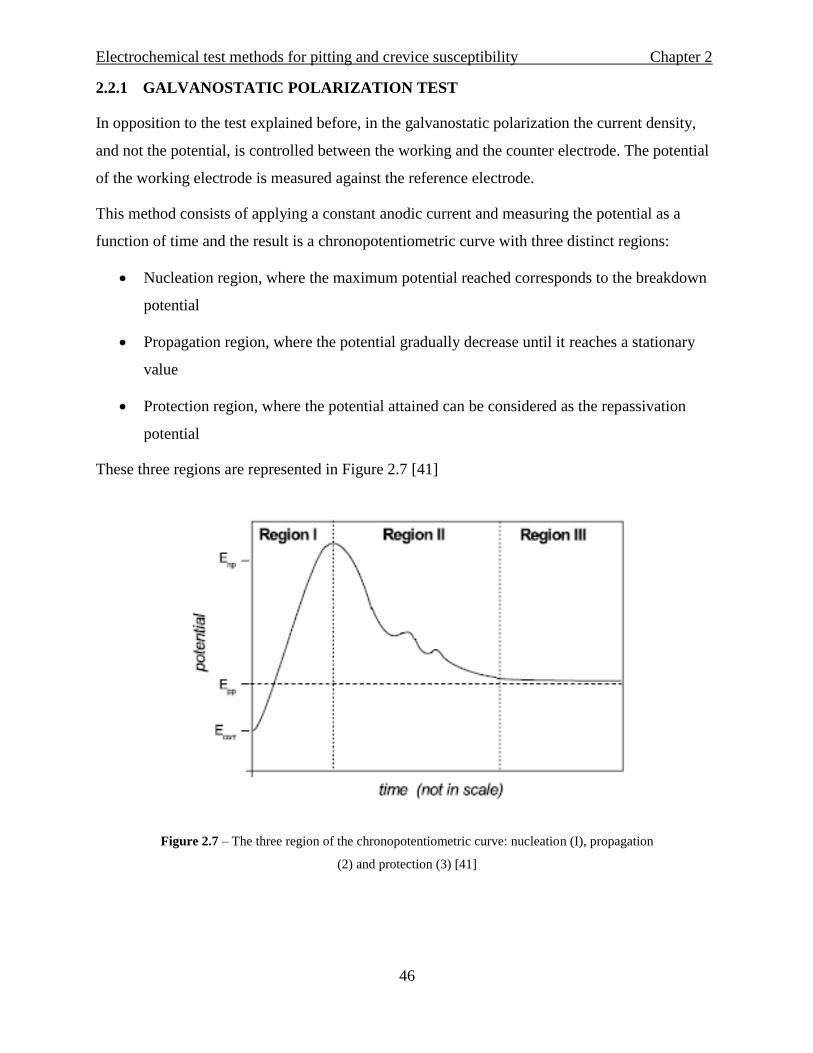
Table 4.6 Results for potentiostatic polarization at 0,335 V vs Ag/AgCl/KClsat, addition of 100
ppm every day (first 62 days) and 500 ppm every two days, surface area of 2 cm2, room temperature
Table 4.6 Results for potentiostatic polarization at 0,335 V vs Ag/AgCl/KClsat, addition of 100
ppm every day (first 62 days) and 500 ppm every two days, surface area of 2 cm2, room temperature

Introduction___________________________________________________________________________Chapter
1Index of Figures
10
ABSTRACT ITALIANO
Gli acciai inossidabili sono ampiamente utilizzati in ambienti aggressivi grazie alla loro
resistenza alla corrosione, dovuta alla presenza di uno strato superficiale composto da ossidi
misti, chiamati film passivo. Nel caso specifico degli acciai inossidabili il comportamento
passivo è concesso dalla presenza di cromo, almeno il 10,5% definito dallo standard, e dalla
presenza di una frazione minore di altri elementi per migliorarne le qualità, quali nickel,
manganese, molibdeno. Tuttavia questo tipo di acciai può soffrire di attacchi di corrosione
localizzati, nello specifico attacchi di vaiolatura e di corrosione in fessura, e sono necessari
strumenti pratici per selezionare materiali per specifici ambienti corrosivi in funzione dei
contenuti di cloruri, della temperatura e di altri parametri.
Cruciale è la valutazione del potenziale di rottura del film, chiamato Epit o Eloc, e potenziale di ri-
passivazione, Eprot o Erep, variando i parametri dell’esperimento. Ciò può essere ottenuto usando
un test di polarizzazione potenzio-dinamica (per valutare entrambi i potenziali in funzione del
contenuto di cloruri) sia le prove di polarizzazione potenzio-statica (per valutare il contenuto di
cloruri critici rispetto al potenziale di polarizzazione).
I dati raccolti sono stati utilizzati per costruire una mappa di corrosione con Potenziale (vs
Ag/AgCl/KClsat) rispetto al contenuto di cloruri. Questa mappa è stata proposta da Pietro
Pedeferri per l'applicazione di protezione o prevenzione catodica nei calcestruzzi armati in
presenza di cloruri.
L'importanza del diagramma Pedeferri sta nella sua capacità di prevedere le zone di protezione in
caso di presenza di corrosione e di ri-passivazione per un certo potenziale e per determinati
parametri ambientali. La deviazione standard dei potenziali di interesse è stata studiata in
funzione di diversi parametri ambientali (contenuto di cloruri), di set-up (velocità di scansione
del potenziale) e geometrici (diversa area superficiale).
La tesi è strutturata in sei capitoli:
Introduzione
Metodi elettrochimici
Materiali e strumentazione
Risultati

Introduction___________________________________________________________________________Chapter
1Index of Figures
11
Discussione
Conclusione
Questa tesi è il proseguo di una tesi precedente, i cui risultati sono utilizzati sono utilizzati nel
Capitolo 5: Discussione.

Introduction___________________________________________________________________________Chapter
1Index of Figures
12
ABSTRACT
Stainless steels are widely adopted in corrosive environments and their resistance to corrosion due
to the presence of a superficial layer composed by mixed oxides, called passive film. In the case
of passive film the passive behaviour is granted by the presence of chromium, at least 10,5%
defined by the standard, and the presence of smaller fraction of other elements to enhance this
behaviour. Nonetheless, they may suffer of localized corrosion attack, i.e. as pitting and crevice,
and practical tools are needed to select materials for specific corrosive environments as a function
of chlorides contents, temperature and other parameters.
Crucial is the evaluation of the breakdown potential, Eloc, and repassivation potential, Erep, by
varying the chlorides content of the solution. This can be achieved using potentiodynamic
polarization test (to evaluate both potential respect a chloride content) and potentiostatic
polarization tests (to evaluate the critical chloride content respect to the polarization potential).
The data collected have been used to build a corrosion map with Potential (vs SSC) vs Chloride.
This map have been proposed by Pietro Pedeferri for the application of cathodic protection or
prevention in a concrete in presence of chloride.
The importance of Pedeferri diagram stays in its capability of predict pitting and protection
potentials ranges where pitting corrosion and repassivation occur for a certain potential and for
certain environmental parameters. The data deviation of Eloc and Erep was studied, along with that
of corrosion potential, Ecorr.
In line with the theoretical explanation, the results showed that the mean values and the data
deviation of the three mentioned potentials was decreasing with increasing chloride contents.

13
Chapter 1
INTRODUCTION
1.1 BASICS OF CORROSION: THE ELECTROCHEMICAL MECHANISM
A generic corrosion reaction for a metal (Me) can be schematized as follows
Eq 1.1 Me + environment→ Me corrosion products
When the environment is an electrolyte solution, the overall corrosion reaction involves a metal
oxidation process and the reduction of the oxygen dissolved in the solution or in the case of acid
solutions the reduction of hydrogen occurs; in the case of iron:
Eq 1.2 Iron + oxygen + water → corrosion products (rust)
Eq 1.3 Iron + acid solution → iron ions + hydrogen
These two reaction (Eq 1.2 and Eq 1.3) proceed according to an electrochemical mechanism
involving the electrons of the metallic material. The reaction is the sum of two complementary
electrode processes: an anodic process involving the oxidation of the metallic material, which
makes electron available in the metallic phase, and a cathodic process which consumes the
electrons that are made available in the anodic process through a reduction reaction of molecular
oxygen, hydrogen ions or both.
The generic anodic process of a metal can be represented by the oxidation reaction of a metal to
its ion which passes into solution (Eq 1.4) or, in some cases, the metallic material tends to form
hydroxides (Eq 1.5).
Eq 1.4 Me → Mez+ + ze-
Eq 1.5 Me + zH2O → Me(OH)z + zH+ + ze-
Where Me is a generic metal, Mez+ is the metal ion that passes in the solution, z is the valence of

Introduction___________________________________________________________________________Chapter
1Index of Figures
14
the metal, e- indicates the electron and H+ indicates the hydrogen ions.
By contrast, the cathodic process that are of practical interest in corrosion are limited. In case of
corrosion in acidic solution, the cathodic process is the reduction of hydrogen ion and the
production of molecular hydrogen, according to reaction Eq 1.6. In natural environments, the
predominant reaction is the oxygen reduction, which can be distinguished in two different reactions
depending if it is a neutral or basic environment (Eq 1.7) or in acidic environment (Eq 1.8).
Eq 1.6 2H+ + 2e- → H2
Eq 1.7 O2 + 2H2O + 4e- → 4OH-
Eq 1.8 O2 + 4H+ + 4e- → 2H2O
The oxygen which appears as a reagent is a molecular oxygen dissolved in water, whose
concentration ranges from 0 to 12 ppm.
Since the electroneutrality must be maintained, the two reactions must occur simultaneously and
with the same velocity (Fig 1.1) [1].
Figure 1.1 – Schematic of the current circulation during a corrosion process, with the expression of the
electroneutrality
1.2 THERMODYNAMIC AND KINETICS OF CORROSION
The fundamental questions that must be answered in corrosion is if the metal can be corroded in
such a solution and, if the answer is yes, how fast the corrosion rate is.
To answer the first question, it is to point out that corrosion reaction for a metallic material occurs

Introduction___________________________________________________________________________Chapter
1Index of Figures
15
if it is thermodynamically favoured: in other words if the variation of the free energy ΔG associated
to it is negative. If it is considered a corrosion reaction of two complementary anodic and cathodic
reaction, for example Eq 1.4 and Eq 1.7, the general thermodynamic condition outlined can be
applied to the reactions. Since these are electrochemical reactions, the variations of Gibbs free
energy can be expressed as the variation of the electro-motive force associated with the reaction
(Eq 1.9):
Eq 1.9 ΔG = -zFΔE
Where ΔE is the electromotive force of the reaction considered, z is the valence of the metal and
F is the Faraday constant. For sake of simplicity, ΔE can be thought as the difference of the
cathodic reaction potential and the anodic reaction potential. So, if the Gibbs free energy have to
negative, ΔE have to be positive for the spontaneity of the reaction: this means that the cathodic
reaction have to be nobler than the anodic reaction.
In 1946 Marcel Pourbaix introduced a potential-pH diagram which plot the equilibrium potentials
as the pH varies for metal in contact with electrolytes. In this diagram (Fig 1.2) the two possible
cathodic reactions, i.e hydrogen release and oxygen reduction, are represented by two parallel lines
with an angular coefficient of -0,059 and a distance of 1,23 V, which are obtained by the
corresponding Nernst equations, with the line a) being the hydrogen evolution and line b) being
the oxygen reduction. In the interval between the two lines the water stability is defined, while
below the hydrogen release there is the stability region of the molecular hydrogen an above the
oxygen reduction, the molecular there is the molecular oxygen stability region. The metal
dissolution is represented in this diagram with horizontal lines, depending on its ions concentration
in the solution. It is to point out that while the cathodic reactions are pH dependant, the anodic
ones are pH independent. Each horizontal line divides the plane in two regions: the upper part
corresponds to the corrosion regions, while the lower part is the thermodynamic stability region,
also known as the immunity zone.

Introduction___________________________________________________________________________Chapter
1Index of Figures
16
In the simplest case, if dissolution reaction of the metal leads to the formation of hydroxides, which
occurs especially in the neutral o basic environment, can be derived that the equilibrium condition
varies with the pH (Eq 1.10)
Eq 1.10 pHEE zz OHMMOHMM
eq 059,0)(/
0
)(/
The Pourbaix diagrams, which are constructed on the bases of thermodynamic equilibrium data
for electrochemical reactions involving the metal as pH varies, show the stability zones of the
chemical species involved: immunity zone of the metal, the stability zone for oxides, which may
lead to passivation phenomena, the stability zones of the metal ions. So it can be used to determine
the thermodynamic condition of the system, but cannot give the information on the kinetics of the
processes.
The availability of driving force represents a necessary, but not sufficient, condition or the
corrosion reactions to take place: the reactions resistances condition the corrosion rate may delay
of stop the corrosion.
To describe a corrosion system it is opportune to use Evans diagram, proposed by U.R. Evans in
1945. In this diagram the two axis represents the potential (E) and the current density, in logarithm
scale (log j or log i). As shown in Fig 1.1, the current circulating in the cell must be conserved: so
the current of the anodic reaction have to be equal to the current of the cathodic one. This diagram
show the characteristic curves of the anodic and cathodic reactions obtained experimentally (Fig
1.3) starting from the reaction’s equilibrium potential (Eeq,a Eeq,c). As the current increases, the
Figure 1.2 – Pourbaix diagram for a generic metallic material M which forms hydroxides [2]

Introduction___________________________________________________________________________Chapter
1Index of Figures
17
reaction potential shifts: for anodic reaction the shift is positive, for the cathodic one is negative.
Eventually the two curves, if plotted in the same diagram, will meet and the corrosion potential
(Ecorr) and the corrosion rate (log icorr) are then calculated (Fig 1.3) [2].
As said before in the Pourbaix diagram, if an oxide or hydroxides is present, so the metal in in the
stability zone of that state, passivation phenomena can occur.
When iron, as also carbon and low alloy, are in natural (soils and water) or acid solutions, it is in
the so-called active condition (Fig 1.3). In these cases the anodic process cannot contribute in the
reducing of corrosion rate. Numerous metals, and their alloys, with an high affinity for oxygen
have the characteristics of covering themselves with a protective layer of oxides, which prevents
their corrosion in a corrosive environment. This condition is called passivity and unable the metal
to behaves as a nobler metal. The anodic curves of these metals has a characteristic shape, in which
one can distinguish three zones: the activity zone, the passivity zone and the transpassivity zone
(Fig 1.4) [2].
Figure 1.3 – Evans diagram for a generic corrosion process: anodic (blue) and cathodic (red) processes [2]

Introduction___________________________________________________________________________Chapter
1Index of Figures
18
In the figure above three potentials can be distinguished and they delimit the three zones mention
above: from the equilibrium potential to the passivation potential (Ep) there is the activity zone, in
which the metal behaves as a normal active metal. From the passivation potential to the
transpassivity potential (Et) the passivity region is determined, where the corrosion process is slow
down to a negligible corrosion rate (jp<50 µm/year [2]). Above the transpassivity potential the
transpassity region starts: in this region the oxides layer is no more protective.
Actually, even if a metallic material is passive, it can undergo some sort of corrosion on a very
small part of the metallic surface compared to the exposed area: the two corrosive attacks that are
of interest in this work are the pitting and crevice phenomena.
1.3 PITTING AND CREVICE CORROSION OF STAINLESS STEELS
When the anodic and cathodic reactions take places o different surfaces, localized corrosion occurs,
affecting only a limited art of the surface exposed to the environment [2]. The separation of the
areas leads to the circulation of a current with the circulation of the electrons in the metal from the
anodic to the cathodic surfaces and the circulation of ions in the solution. Pitting and crevice
corrosion are part of this type of corrosion.
Pitting manifests itself as attacks, leaving pits o cavities, which are extremely penetrating but affect
only a very small part of the metallic surface. All metals that exhibit an active-passive behaviour
Figure 1.4 – Evans diagram for a generic anodic process of a passive metal [2]
Introduction___________________________________________________________________________Chapter
1Index of Figures
19
can be subjected prone to pitting corrosion, although most experimental studies have involved
stainless steels, aluminium, and copper. Pitting is caused by the presence of aggressive anions in
the electrolyte, usually Cl- ions are considered when stainless steel or aluminium are considered.
The chloride ion has a special importance in pitting corrosion for two main reasons: Cl− ions are
ubiquitous, being constituents of seawater, brackish waters, de-icing salts and secondly the
chloride ion is a relatively small anion and has a high diffusivity [4].
The tendency of a metal or alloy to undergo pitting is characterized by its critical pitting potential,
as illustrated in Fig 1.5. In the absence of chloride ions, the metal retains its passivity up to the
electrode potential of transpassivity. In the presence of chloride ions, the passive film suffers
localized attack, and pitting initiates at a potential called pitting potential or breakdown potential
[4]. Once corrosion pits initiate, they usually propagate rapidly, as shown by the sharp rise in
current density at electrode potentials just beyond the critical pitting potential.
Figure 1.5 - Schematic anodic polarization curve showing the critical pitting potential (for a passive
metal) [3].
The critical pitting potential, Epit or also called Eloc the thesis, is a characteristic property of a given
metal or alloy in a given environment. For a given chloride concentration, the more positive the
critical pitting potential, the more resistant the metal or alloy to pit initiation [4].
The significance of the pitting potential is that below Epit, pitting does not manifest (E < Epit)
while above Epit, corrosion pits initiate and propagate. (E > Epit)

Introduction___________________________________________________________________________Chapter
1Index of Figures
20
Moreover not only there is not only a threshold in the potential, but also in chloride
concentrations [5]: actually a critical chloride concentration for a given potential can be
observed, as depicted in Fig 1.6 [2].
Figure 1.6 – Dependence of pitting potential in function of the chloride contents [2]
1.3.1 MECHANISM OF PIT INITIATION
Pitting corrosion may be divided into initiation and propagation stages. It is considered that the
initiation stage includes both the breakdown of the passive film and the onset of an anodic current
at the metal surface. The three-main possible pitting mechanism include the penetration
mechanism, the adsorption mechanism and the film rupture mechanism [2, 3].
In the penetration mechanism, aggressive anions are transported through the oxide film to the
underlying metal surface where they participate in localized dissolution at the metal/oxide
interface. This mechanism is depicted schematically in Fig 1.7. The mechanism by which Cl− ions
penetrate the oxide film is not completely understood, but the radius of the Cl− ion is only slightly
larger than that of an oxygen ion (1.81 vs. 1.40 Å, respectively), so that Cl− migration through
oxygen vacancies is a possible mechanism of chloride entry into the passive film [6].

Introduction___________________________________________________________________________Chapter
1Index of Figures
21
Figure 1.7 - Penetration mechanism of pitting corrosion [6].
In the film thinning mechanism, the aggressive anions, in particular chlorides, first adsorb on the
oxide surface and then form surface complexes with the oxide film which lead to local dissolution
and thinning of the passive film, as shown schematically in Fig 1.8.
Figure 1.8 - Film thinning mechanism of pitting [6].
In the film rupture mechanism (Fig 1.9), chloride ions penetrate the oxide through cracks or flaws
in the film. In addition to pre-existing defects in the oxide film, flaws may further develop by
hydration/dehydration events in the oxide film and by the intrusion of Cl− ions into the film. It has
been said that the presence of a high electric field in the oxide can lead to an electromechanical
breakdown of the passive film. It should be noted that pre-existing flaws cannot extend down to
the underlying metal substrate because the metal would quickly react with water molecules in the
electrolyte and would re-oxidize. Then, chloride ions must penetrate the re-formed oxide film by

Introduction___________________________________________________________________________Chapter
1Index of Figures
22
mechanisms discussed above. Passive films can also be ruptured or disrupted due to metallurgical
variables, such as grain boundaries, impurity atoms, and inclusions.
Figure 1.9 - The film rupture mechanism of pitting [7].
These three mechanisms of pit initiation (chloride penetration, film thinning, and film rupture) are
not necessarily mutually exclusive.
1.3.2 MECHANISM OF PIT PROPAGATION
The mechanism of pit propagation is shown in Fig 1.10. When the corrosion pit has started, the
corresponding local current density is very high because the current is confined to a small active
geometrical area, while the oxide film adjacent to the pit remains passive and act as cathode. As
the pit grows, its volume is increased, but dissolved metal cations are confined within the pit and
do not diffuse out into the bulk electrolyte due to the confinement of a restricted geometry or a cap
of porous corrosion products, which in some cases can be formed. As a result, accumulated metal
cations undergo hydrolysis, as in the case of crevice corrosion, and a local acidity develops within
the pit. Finally, the H+ ions and cations are accumulated within an active pit and the Cl− ions
migrate from the bulk electrolyte to the electrolyte in order to maintain charge neutrality within
the pit solution [7].
Hence the propagation stage of pitting, involves the formation of a highly corrosive internal
electrolyte which is acidic and concentrated in chloride ions and in dissolved cations of the metal
or alloy. When the corrosive pit electrolyte has been formed, pitting is considered to be
autocatalytic in nature.

Introduction___________________________________________________________________________Chapter
1Index of Figures
23
Figure 1.10 - Schematic representation of the propagation stage of pitting [3].
Even at lower potential than the pitting potential, localized attack can occur. These are
metastable pits, which can evolve into pits and then propagate, or repassivated.
1.3.3 CREVICE CORROSION MECHANISM
Crevice corrosion can occur in geometrical clearances (under gaskets or seals, under bolt heads,
between overlapping metal sheets, within screw threads, within strands of wire rope) under
deposits (corrosion products, dust particles). A necessary condition to have crevice attacks is to be
in a chloride containing environment
As for pitting, even for crevice corrosion two distinct stages can be defined: initiation and
propagation.
1.3.4 INITIATION OF CREVICE CORROSION
Crevice corrosion initiates due to the operation of a differential oxygen cell. Oxygen reduction
occurs both on the metal surface which is exposed to the bulk electrolyte and also on the portion
of the metal surface which is contained within the crevice, as depicted in Fig 1.11. The cathodic
reaction is the same on both internal and external metal surfaces.
The metal exposed to the bulk electrolyte is in contact with an open supply of oxygen from the
atmosphere, so as O2 is consumed near the external metal surface, additional O2 molecules diffuse

Introduction___________________________________________________________________________Chapter
1Index of Figures
24
to the metal surface and a steady-state concentration of O2 is maintained near the surface of the
external metal. However, when O2 molecules are consumed within the narrow clearance of the
crevice, they are not easily replaced due to the long narrow diffusion path formed by the crevice
[7].
Figure 1.11 - Schematic illustration of the initiation stage of crevice corrosion: (c) is an expanded view of
(a) and (b) [3].
1.3.5 PROPAGATION OF CREVICE CORROSION
Crevice corrosion propagates by changes in the electrolyte composition within the crevice. In
particular, the crevice electrolyte will become acidic in nature and will also contain concentrated
amounts of cations discharged from the metal or alloy. In chloride solutions, the internal electrolyte

Introduction___________________________________________________________________________Chapter
1Index of Figures
25
within the crevice will also become concentrated in chloride ions. This internal electrolyte is
sufficiently aggressive to break down the passive film on the metal. These changes in the
composition of the crevice electrolyte occur because of the narrow geometrical character of the
crevice, which allows only restricted exchange between the crevice and bulk electrolytes [8].
Figure 1.12 - Schematic illustration of the propagation stage of crevice corrosion of iron [5].
The propagation stage of crevice corrosion, like that of propagation of pitting, involves the
formation of a highly corrosive internal electrolyte which is acidic and also concentrated in
chloride ions and dissolved cations of the metal or alloy, as shown in Fig 1.12. As for pitting, also
the initiation stage of crevice corrosion can be quite prolonged (months to years), but propagation
may proceed rapidly due to the highly corrosive crevice environment which is formed [6].
1.4 EFFECT OF METALLURGICAL FACTORS
Stainless steel are iron-chromium-carbon based alloys and containing other elements like nickel,
molybdenum, manganese, nitrogen, tungsten etc. which make them more resistant to corrosion.
The standard UNI ENI 10088-1 defines stainless steels as iron based alloys which contains at least
10.5% of chromium.
Depending on the alloying elements, and so the microstructure, one can divide all stainless steels
in three different families: austenitic (FCC), ferritic (BCC), martensitic (TCC), duplex (both
austenitic and ferritic phases). Seeing the Fe-Cr and Fe-Ni (Fig 1.13) diagram states that some
alloying elements tend to enlarge the α-phase while other tends to enlarge the γ-phase; combining
the effect of these elements and the Ni equivalent and Cr equivalent contents are obtained.

Introduction___________________________________________________________________________Chapter
1Index of Figures
26
These two equivalent number are used in the Schaeffler diagram to define the microstructure (Fig
1.13).
Figure 1.13– Schaeffler diagram
1.4.1 CHEMICAL COMPOSITION OS THE STAINLESS STEEL
As already said, all stainless steel have at least 10,5 % of Cr in their composition to make them
more resistant to general corrosion. It is common knowledge [9] that going in more basic solution,
the carbon steel becomes more resistant to corrosion and at pH for 12,5 it becomes completely
passive; so the Cr addition helps the steel not only to become more corrosion resistant in general,
but specifically at pH lower than 11.
Existing data show that Cr, as for Mo, increase the pitting resistance of steels in chloride solutions;
this alloying element does not only reduce susceptibility to pit nucleation (Fig 1.14), but also
diminish the rate of pit development [4].

Introduction___________________________________________________________________________Chapter
1Index of Figures
27
Figure 1.14– Pitting potential of Cr in the Fe-Cr alloys in 0,1 M NaCl at 25°C [4]
It can be seen that, for moderate anodic polarizations in acidic solutions, the passive film consists
essentially of chromium in its trivalent state. As the potential increases above the stability limit of
chromium III, (about 0.6/0.8 VSHE), the passive film will start to change composition and the
fraction of trivalent iron in the film will increase. For acidic solutions, the cation fraction of Cr in
the passive film normally amounts to 50/70%. For basic solutions, the solubility of Cr increases,
resulting in a higher fraction of iron.
Nickel is less readily oxidized than iron and chromium [13]. Consequently, there is an enrichment
of Ni in its metallic state in the metal closest to the oxide/metal interface. This enrichment could
assist in the formation of a nickel nitride. Nickel could also bring down the overall dissolution
rates of Fe and Cr.

Introduction___________________________________________________________________________Chapter
1Index of Figures
28
Figure 1.8– Pitting potentials for the Fe-15Cr alloys with increasing Ni content in 0,1 M NaCl at 25°C [4]
Molybdenum is an alloy element with a strong beneficial influence on the pitting resistance of a
stainless steel [14]. When included as an alloying element in a stainless steel, molybdenum is
incorporated into the passive film, showing a complex oxide chemistry with different states of
oxidation. Hexavalent Mo is found to be enriched at the surface, whereas tetravalent states show a
more homogeneous distribution through the film. There are two possible hexavalent states: MoO3,
which is soluble in acidic eletrolytes and MoO42- which shows a higher stability. Distinguishing
between these two states is difficult even with a high resolution XPS spectrometer.
Tungsten is fairly recent as a major alloying element in commercial stainless steels. It has been
attributed properties similar to those of molybdenum. An important difference between tungsten
and molybdenum oxides lies in the different stability of their oxides in acid solution. While
hexavalent molybdenum oxide dissolves at potentials well below oxygen evolution, the stability
of hexavalent tungsten oxide extends to anodic potentials of several tens of volts.

Introduction___________________________________________________________________________Chapter
1Index of Figures
29
Nitrogen is the element attributed the strongest beneficial influence on localised corrosion in the
pitting resistance equivalent formula (PREN). As for molybdenum, nitrogen also shows strong
concentration gradients in the passive film [15]. A possibility is the formation of a nitride at the
metal/film interface which brings down the dissolution rates for the individual elements in the
alloy [16]. Nitride has also been put forward as a possible mechanism for synergy between nitrogen
and molybdenum.
Recently, addition of Mn to stainless steel has been used to increase the solubility of nitrogen and
molybdenum, both of which have a strong beneficial influence on the pitting resistance [12].
To compare different stainless steels and to have a qualitative evaluation of the resistance of the
stainless steel in a chloride containing solution can be used the PREN (Pitting Resistance
Equivalent Number).
This number can be evaluated with the following equations, depending on the composition of the
stainless steel:
Eq. 1.1 NMoCrPREN %16%3,3%
Eq. 1.12 NWMoCrPREN %16)%5,0(%3,3%
The first equation is used when the content of Mo is less than 1,5% , while the second takes into
account also the presence of W when the content of Mo is more than 1,5%.
All the equation above are used for austenitic stainless steel, if other type (ferritic or martensitic),
the coefficient which multiply the contents of the different alloying elements.
The effect on pitting potential of the various alloying elements is shown in Table 1.1 [4]
Table 1.1 – Approximated effect of the major alloying elements [4]
Alloying element Content (max) Eloc shift (max)
Mn 11 50
Ni 25 200
Cr 30 900
Mo 4,5 900
.

Introduction___________________________________________________________________________Chapter
1Index of Figures
30
1.4.2 STEEL MICROSTRUCTURE AND METALLURGICAL DEFECTS
In general can be said that the resistance of the passive film to the breakdown is related to the
properties of the base metal. If zones adjacent to the grain boundaries are impoverished in
chromium, and this does occur in sensitized stainless steels for example, the passive film is less
protective in these regions and localized corrosion is likely to occur.
Also, at sites where non metallic inclusions emerge on the metal surface, the film is weaker and
pits may nucleate [4]. For example the vicinity of MnS inclusions is known as a preferential
location for pit nucleation on stainless steels in the presence of aggressive ions like chlorides. The
pitting susceptibility of MnS in chloride containing solutions is often attributed to the preferential
adsorption of chloride ions on MnS rather than on the surrounding passive metal, leading to a
decrease in the activation potential of the inclusion [17].
Mechanisms have been proposed to explain the role of the MnS inclusions on pitting initiation
[18]. Nevertheless, the phenomenon is subject of intense discussion. Schmuki et al [19]
demonstrated that corrosion can start around or inside the inclusions, in high oxidising
environments, and also that some of the inclusions can remain inactive, even in very oxidising
conditions. Pitting attack, in or around inclusions, depends upon several factors such as inclusion
composition, shape and geometry.
1.4.3 COLD WORKING
Austenitic stainless steel is used in various applications not only due to its high corrosion resistance
but as well for its good ductility.
However, the application of these types of steel is limited due to its low yield strength (about
200MPa), hence the focus is to find some methods to provide ultrafine-grain (UFG) in order to
attain a higher strength without losing the ductility and the corrosion resistance that are
characteristic of this type of material [4]. To achieve UFG there are three different families of
process that can be used: severe plastic deformation (SPD), advanced thermomechanical process
(ATP), mechanical milling (MM) called also shot-peening.
A study [20] say that the cold working affect the pitting initiation frequency: essentially the
frequency of initiation increase with the increase of the cold-rolling reduction (Fig 1.9). The

Introduction___________________________________________________________________________Chapter
1Index of Figures
31
frequency of initiation have been measured as the number of metastable pits.
Figure 1.9 – Effect of cold rolling on AISI 304 in 0,1 NaCl + 2x10⁻⁴ FeCl3 [20]
1.4.4 SURFACE FINISHING AND ROUGHNESS
One major technological concern associated with the electrochemical behavior of stainless steels
is the surface finishing.
This has been found to affect the corrosion resistance of stainless steels being related to different
forms of localized corrosion, such as stress corrosion cracking and pitting corrosion.
It has been seen that the pitting potential decrease as the surface becomes rougher, indicating a less
stable condition owing to localized corrosion. Actually the surface roughness cause a local
weakness in the protective oxide layer, where a critical Cl- concentration can be attained and so
the number of active siter for pit nucleation can increase.
This effect would be related to the so-called openness of the pit, which is related to the aspect ratio
of surface groove: smoother surfaces are characterized by high aspect ratios and are more resistant
to pitting corrosion.

Introduction___________________________________________________________________________Chapter
1Index of Figures
32
This is explained by saying that the metastable pitting is a diffusion-controlled process where the
metal dissolution depends on the concentration of chlorides and of corrosion products inside the
pits [4].
Higher aspect ratios of surface grooves decrease the chloride concentration inside the pits, thus
leading to a reduced current density, and therefore decreasing the pitting nucleation rate [21]. Fig
1.10 show how different surface finishing operations influence the pitting potential for AISI 304.
Figure 1.10 - Potentiodynamic polarization curves for AISI 304 stainless steel samples submitted to
different surface finishing operations in 0,1 M NaCl at room temperature; potential is taken respect to
Ag/AgCl/KClsat reference electrode [21]
As shown in the picture, it is clear that the pitting potential of the as-received sample is lower than
the others, meaning that it is more prone to have pitting attacks.
Also in another paper [22] the same trend, as shown in Fig 1.11. The specimen 2B is to be
considered the untreated sample.

Introduction___________________________________________________________________________Chapter
1Index of Figures
33
Figure 1.11 - Potentiodynamic curves for four different surface finishing of AISI 304 stainless samples in
0,5 M NaCl, san rate of 1 mV/s [22]
Even if no big difference can be noticed for the treated samples, a clear difference can be seen with
the as-received sample.
1.5 EFFECT OF ENVIRONMENTAL FACTORS
Pitting initiation depends not only on the chemical composition and on microstructure of the
material that has to bear this kind of corrosive attack, but also on the type of environment that
surround it.
Four major environmental factors can be took into account:
Chloride concentration
Temperature
pH
Flow rate
The general trend is that increasing the chloride concentration, decreasing the pH, increasing the
temperature and increasing the flow rate the pitting potential lowers.

Introduction___________________________________________________________________________Chapter
1Index of Figures
34
1.5.1 Chloride concentration
As already mentioned in the section of 1.2 (Pitting and crevice corrosion in stainless steel) the
effect of chloride content on pitting susceptibility of stainless steel has been widely investigated
[24] and it is well established that it decrease the pitting potential (Fig 1.6 and Fig 1.12).
It is suggested that transition between passivity and pitting can be explained by a competitive
adsorption mechanism in which chloride ions move into the the oxide/liquid interface and be able
to displace the adsorbed oxygen species.
The chloride tends to reduce the passivity region of the anodic curve of stainless steel reducing the
pitting potential.
The anodic processes associated with a metal depassivation are strongly affected by the chloride
concentration in the solution: a large amount of chloride the passive film becomes susceptible to
pitting corrosion and can suffer localized damage; a simple equation can be found that correlate
the pitting potential, Epit, with the concentration of chlorides:
Eq. 1.14 ClBAEpit log
Where A and B are constants that depends on both environmental and metallurgical condition [4].
Figure 1.12 – Effect of Cl- to the pitting potential

Introduction___________________________________________________________________________Chapter
1Index of Figures
35
1.5.2 TEMPERATURE
A decrease of the pitting potentials at high temperature has been seen and can be explained by a
more intense agglomeration and stronger chemisorption of chloride ions on the metal surface,
causing easier breakdown of passivity. The pit number also increases with increasing temperature
because at higher temperature more site are susceptible to pit nucleation. An increase in
temperature accelerates the transport of reagents and reaction products to or from the electrode.
However, the effect of temperature on transport rate is considerably less than the effect on the
chemisorption of chloride ions and on the ionization of metal. Therefore, the changes in the
electrolyte concentration inside pits occurs more rapidly with increasing initial current density in
pits. These concentration changes lead to increased concentration polarization, and to ohmic
polarization, when salt layers or other corrosion products are deposited in pits. Consequently,
inhibition of the metal dissolution, both by transport processes and decreases of the current density
in pits vs exposure time, are more pronounced at higher temperatures. It is notable that at certain
temperatures, pitting can occur without chloride ions, which is presumably related to some changes
in film structure at these temperatures [4].
Fig 1.13 [25] shows how the pitting potential varies with varying the temperature for the Alloy
600, a nickel based alloy. As can be seen there is a clear dependence of pitting potential respect to
the temperature.
Figure 1.13 – Effect of the temperature on the pitting potential of Alloy 600 in deaerated 0,282 m NaCl
solution [25]
Another study [26] that the combination of an high temperature and the presence of chloride favour

Introduction___________________________________________________________________________Chapter
1Index of Figures
36
the breakage of the film.
1.5.3 pH
It is known that the pH of the solution directly affects the cathodic process of hydrogen evolution,
but pH also has a strong influence on the kinetics of the anodic processes through the solubility of
corrosion products and their protective properties [27]. A lot of studied showed that the pitting
potential becomes lower as the pH is more acidic, while at high pH values pitting potential is
moved in the noble direction, because of the inhibition effect due to a higher concentration of OH-
ions (Fig 1.14).
Figure 1.14– Effect of pH on pitting corrosion [30]

Introduction___________________________________________________________________________Chapter
1Index of Figures
37
A study [28] reported that values below 2,2 are important for pitting corrosion: actually they
claimed that no much difference in pitting potential between 2,2 and 5 pH is seen.
As said before, higher values of pH have an inhibiting effect on the pitting corrosion, as the tests
done for pH ranging from 4 to 9 show [29].
1.5.4 SOLUTION FLOW
Pitting of stainless steels is often associated with stagnant conditions, but with the increasing of
the speed of the solution, positive effects have been detected. Table 1.2 show the results and the
difference between pit initiation when there is a flow of the solution (1,2m/s) from when the water
is still. The metal tested was a welded 316 stainless steel in seawater. No pitting initiate when the
solution is agitated, while attacks appears when the solution is stagnant.
Table 1.2 – Effct of seawater flow rate on pitting of welded AISI 316 after 1257 days if exposure [13]
Material Agitated
Number of pits
Stagnant
Number of pits
316 Plate
weld
0 87
0 47
It is possible to explain this phenomenon by saying that when the solution is in motion the three
mechanism described in section 1.2.1 (Pitting initiation mechanism) are hindered.
1.6 THE PEDEFERRI’S DIAGRAM OF STAINLESS STEELS
Pedeferri diagram illustrates conditions for passivity and corrosion in terms of chloride
concentrations (Fig 1.15). In the specific, Fig 1.15 depict the original Pedeferri’s diagram used to
evaluate the type of cathodic protection of rebars in the concrete in presence of carbonation or in
presence of chlorides [9].
In accordance with Pourbaix diagram, in this diagram three important zones can be individuate:
Perfect passivity, where no pit can initiate or propagate

Introduction___________________________________________________________________________Chapter
1Index of Figures
38
Imperfect passivity, where pits can propagate but not initiate
Pitting, where pits can both initiate and propagate
The definition of these zones has a high industrial values because it makes possible to stop, or even
to make it impossible, the pitting corrosion.
The importance of Pedeferri diagram lays in the capability of predicting the pitting and
repassivation potentials for certain environmental potential.
The
aim
of
this
work is both to evaluate a suitable electrochemical methodology to obtain the Pedeferri diagram
and to evaluate the influence of method parameters (scan rate, chloride content, size of the sample)
for the AISI 304 stainless steel.
Figure 1.15– Pedeferri diagram for the cathodic protection or prevention for the rebars in the reinforced
concrete

39
Chapter 2
.ELECTROCHEMICAL TEST METHODS FOR
PITTING AND CREVICE SUSCEPTIBILITY
MEASUREMENTS
There are various electrochemical methods that can be used to determine the characteristics of
corrosion resistance, which are divided in two main families divided in the use of DC and AC.
The first family can be divided in other two subcategories that are: tests that use as an input a
variation in polarisation potential and the output will be a current and test that use as an input a
current ad the output will be a potential difference
Electrochemical polarization is the change of electrode potential due to the flow of current. The
technique is built on the idea that predictions of the corrosion behaviour of a metal in a specific
environment can be achieved by forcing the material away from its steady state condition and
monitoring how it responds to this displacement.
In the second family one method is the most known: the electrochemical impedance spectroscopy
(EIS).
In all these types of test the conductivity of the electrolyte is a very important factor that should
be considered, because the electrolyte resistance can cause potential drop between the working and
the reference electrode and may cause errors. This effect has an important impact on the
interpretation.

Electrochemical test methods for pitting and crevice susceptibility Chapter 2
40
2.1 MEASUREMENTS WITH A POTENTIOSTAT
The first family of tests, where the control is on the potential, can be divided in three types of
possible method:
Potentiodynamic, where the potential is changed continuously at a constant rate
Quasi-stationary, where the potential is changed stepwise at a desired rate
Stationary, where the potential is held at an assigned potential
2.1.1 CONTINOUS POTENTIODYNAMIC POLARIZATION
In this case the potentiostat is controlled with a computer, which control the change of the
potential, which is called potential scan rate.
The potentiodynamic polarization are performed using the three electrode configuration, which
are: working electrode, reference electrode and counter electrode.
The working electrode is the sample to analyse and it is the electrode to polarize, the reference
electrode is the one that monitor and provide the zero for the potential measurements, the counter
electrode supply the needed current to the working electrode and close the electrochemical
circuit.
Figure 2.1 – Plot of a potentiodynamic polarization [31]

Electrochemical test methods for pitting and crevice susceptibility Chapter 2
41
The system works by maintaining the potential of the working electrode at a specific potential,
that will change in time, with respect to the reference electrode by adjusting the current supplied
by the counter electrode. In the case of localized corrosion the curve is generally analysed in
terms of free corrosion, breakdown or pitting and repassivation potentials (Fig. 2.1 [31]).
The initiation of corrosion is detected when a sudden increase in current density, some order of
magnitude, is observed and the potential at which this phenomenon happens is called breakdown
potential or pitting potential (Epit or Eloc).When the current density reached to a threshold value,
the backward potential scan start. In this way the repassivation potential can be obtained (Eprot or
Erep). The value of this potential has been debated because some authors consider it the potential
at which the current density is zero, others the one at which the forward and backward potential
scan intersect [4, 32]. This type of test can be done also only in the forward potential scans, so to
have a faster test, but only the Eloc can be obtained [33].
One of the regarding on the use of potentiodynamic, both continuous and stepwise, is that the
results of Eloc and of Erep are dependant on the experimental parameters, which the most
important is the scan rate: the higher the scan rate the higher the Eloc is expected. This is due to
incubation process for pitting in which a slower scan rate permits more time for a pit to occur at a
more negative potential during the forward mode [34, 35]. The effect of potential scan rate on the
Epit can be seen clearly in Figure 2.2 [36].
Figure 2.2 – Dependence of breakdown potential on the scan rate [36]

Electrochemical test methods for pitting and crevice susceptibility Chapter 2
42
2.1.2 STEPWISE POTENTIODYNAMIC POLARIZATION
Stepwise potentiodynamic polarization is a method that produces polarization in which the
potential is changed periodically with discrete steps, usually ranging from 25 to 50 mV each
[33].
2.1.3 POTENTIOSTATIC POLARIZATION
Potentiostatic polarization is a long-term test that gives the best information regarding the
localized corrosion of a metal in a given environment because, being at a fixed potential, it
reproduces better the real condition of corrosion. Basically, a constant DC anodic potential is
applied to the sample and the current is recorded as a function of time. When pitting initiate, a
sudden increase in the current density occurs. There are two methods to measure the pitting
potential related to the chloride content of the solution: make tests with a constant chloride
content and define a time limit, initiation time, for the pitting to occur (Figure 2.3), or to make
tests with a varying chloride content, which is added to the solution after a period of time. The
first method is thought to be more accurate in reproducing the environment found in the field
(constant chloride content and potential) but too much time consuming [4].
Figure 2.3 – Current density vs Time depending on the polarization
potential [37]

Electrochemical test methods for pitting and crevice susceptibility Chapter 2
43
While the second method seek to approach the pitting potential in a “horizontal” way. Essentially
in the potentiodynamic test the pitting potential is found increasing the potential and not
changing the chloride contents (vertical way), while for potentiostatic tests the critical chloride
content is found for a specific potential (horizontal way).
Figure 2.4 – Current density vs Time depending on the polarization
potential [38]
As shown in Figure 2.4 [38] when the polarization potential is below the pitting potential, the
current decays to a constant value; on the other hand, when the potential is equal to the pitting
potential or higher, the current increases due to the pits initiation, at the beginning, and growth.
Figure 2.5 – Current density when pitting already initiate depending on the polarization potential: Ea < Eb; plotted vs time [37]

Electrochemical test methods for pitting and crevice susceptibility Chapter 2
44
It has been found [37] that the current density of a stable pit has an increasing trend, until the
polarization is stopped and the pit growth ceased and so the current density returned near zero.
As the Figure 2.5 shows, not only the current density increases when the pit propagates, but also
increases when the potential increases, showing a sharper trend.
It can be concluded that the metal dissolution rate increased significantly with the increasing in
the applied potential, and thus the stable pit would have a faster growth at higher potential.
Even if it is possible to obtain a value for the re-passivation potential using this technique, it is
rarely used.

Electrochemical test methods for pitting and crevice susceptibility Chapter 2
45
2.1.4 COMPARISON BETWEEN POTENTIODYNAMIC AND POTENTIOSTATIC
POLARIZATION
Localized corrosion phenomena has a low reproducibility due to the stochastic nature of the
phenomenon, anyway there are many authors that measured breakdown potential and repassivation
potential using both potentiodynamic and potentiostatic polarization [39, 40].
For example Figure 2.6 shows the results of the potentiodynamic and potentiostatic polarization
curves obtained for UNS S32404.
a)
b)
Figure 2.6 –Potentiodynamic polarization curve (a) and potentiostatic polarization curve (b) obtained for UNS
S32404 [39]
As can be seen the value for breakdown potential are similar: for the potentiostatic test, the current
increase for a value of potential of about 1000 mV SCE, which is also confirmed from the
potentiodynamic polarization curve, which is also easier to read.
2.2 MEASUREMENTS WITH A GALVANOSTAT
The second family can be divided in two different modes: stationary, where the specimen is held
at an assigned current density, quasi-stationary, where the current density is changed stepwise at
a desired rate.
Electrochemical test methods for pitting and crevice susceptibility Chapter 2
46
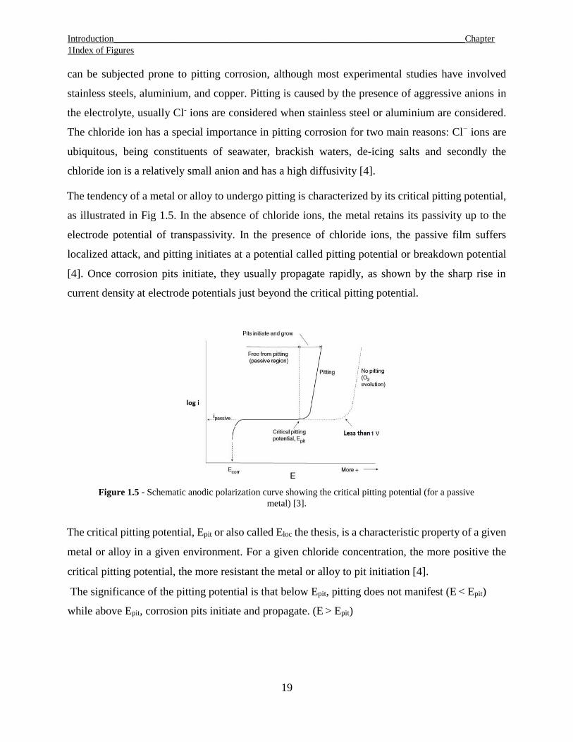
2.2.1 GALVANOSTATIC POLARIZATION TEST
In opposition to the test explained before, in the galvanostatic polarization the current density,
and not the potential, is controlled between the working and the counter electrode. The potential
of the working electrode is measured against the reference electrode.
This method consists of applying a constant anodic current and measuring the potential as a
function of time and the result is a chronopotentiometric curve with three distinct regions:
Nucleation region, where the maximum potential reached corresponds to the breakdown
potential
Propagation region, where the potential gradually decrease until it reaches a stationary
value
Protection region, where the potential attained can be considered as the repassivation
potential
These three regions are represented in Figure 2.7 [41]
Figure 2.7 – The three region of the chronopotentiometric curve: nucleation (I), propagation
(2) and protection (3) [41]

Electrochemical test methods for pitting and crevice susceptibility Chapter 2
47
It has been shown that the galvanostatic method can be used for the determination of breakdown
and repassivation potential without incurring in crevice phenomena [41]: owing to the rapid pit
activation imposed by thi technique, crevice corrosion is eliminated at the specimen/holder
interfaces, even without any specific care in designing electrode holders. This techniques permits
also to have low scattering in the value of pitting potential.
2.2.2 STEPWISE GALVANIC POLARIZATION
In this method, changes in electrode potential are recorded until the breakdown potential is
achieved; at further increase of the current density the potential decrease until a stationary value is
attained and repassivation potential is achieved.
Figure 2.8 shows a curve obtained with this method [4]
Figure 2.8 – Curve obtained with the stepwise galvanic polarization [4]
2.3 ELECTROCHEMICAL IMPEDANCE SPECTROSCOPY
Electrochemical impedance spectroscopy (EIS) is a technique that determines a numerical value
for the degree of corrosion protection provided by the passive film to a metal substrate. This
numerical value is called film impedance and is defined as the ability of the passive layer to resist
corrosion through the combination of barrier and adhesive properties: the more the film protects
the substrate, the higher the impedance value.

Electrochemical test methods for pitting and crevice susceptibility Chapter 2
48
EIS data are collected using a three-electrode cell, which is like the configuration of the
potentiodynamic polarization.
Initially the open circuit potential is determined and is defined as the voltage between the
reference and the working electrode, then a sinusoidal voltage is applied with an amplitude of 10
mV respect to the open circuit potential of the electrochemical cell: this result in a sinusoidal
response. The sample is scanned both over a range of frequencies and a period of time.
There are two limits for the behaviour of the system:
In phase behaviour, which occurs only in pure resistor
Out of phase, which occurs only in pure capacitor
When dealing with AC we can decompose the output signal in two parts: the in-phase
component and out-of-phase component. For sake of simplicity lets think of the input as a
sinusoidal, the in-phase part will be a sinusoidal with the same phase of the input, while the out-
of-phase part will be a sinusoidal with a delay of 90°. Because a passive material contains both
resistive and capacitive elements, the phase shift of the current, and also potential, will be
between 0° and 90°.
The impedance of a sample is determined from the information provided by these two sinusoidal
curves. The impedance can be determined by:
Eq. 2.1 )sin(
)sin(
0
0
i
v
tI
tEZ
Where |E0| and |I0| are the amplitudes of the AC voltage and current, ω is the angular frequencies,
ΦV and ΦI are the phase angles of the voltage and current respectively. From this definition of
impedance, the modulus can be obtain, which is also equal to:
Eq. 2.2
2
.
2 )()( phaseofoutphasein ZZZ
phaseofoutphasein
i iZZeZZ
Where θ is the angle between the real and imaginary axis. The impedance modulus so
incorporates both in phase and out of phase information.

Electrochemical test methods for pitting and crevice susceptibility Chapter 2
49
Impedance data are normally illustrated in Bode plots, with log impedance modulus shown
versus the log of frequency of the imposed signal [43].
This method is efficient at measuring how much the passive layer, or any other protective layer
that has been deposited onto the surface of the sample, is adherent to the substrate: larger the
impedance measured, better the adhesion on the substrate. From these measurements the
thickness of the layer can be obtained [42].
Even if the adhesion and thickness of the passive layer can be used as a qualitative evaluation of
the corrosion protection, this method do not give a numerical value of potential of interest
(pitting and repassivation potentials)
2.4 SCRATCH METHOD
The last electrochemical method presented is the scratch method: in this method the test
specimen is held in the electrolyte at different constant potentials. The protective film is broken
by scratching with a hard material, diamond or carborundum, and then the current density is
monitored to determine whether the metal is capable of repassivation or not. A sharp increase in
repassivation time is usually found at the repassivation potential. The advantage of this method is
that the results are independent on the surface finishing, but the potential measured is usually
nobler than the re-passivation potential but lower than the breakdown potential found with other
methods [4].
In this work two main electrochemical methods, i.e. potentiostatic and potentiodynamic
polarization tests, have been chosen from a vast variety of possible choices. These electrochemical
methods were chosen as an alternative to field testing method as they are less time consuming.

50
Chapter 3
MATERIALS AND METHODS 3.1 MATERIAL The material used as working electrode for the experiment was AISI 304L, UNS S30400,
chemical composition is shown in the Table 3.1
Table 3.1 – Chemical composition of AISI 304L used Fe C Cr Ni Mn Mo N
71,899 0,018 17,271 8,422 1,458 0,076 0,063
This chosen alloy has a PREN around 18.
3.2 SAMPLE PREPARATION
Three types of specimen are chosen for the analysis, with different surface area.
For the most used specimen, an AISI 304 stainless steel plate was cut into rectangular samples in
30x20x2 mm size (in Fig 3.1). Sample preparation for all the tests (potentiodynamic, potentiostatic
and stepwise polarisation) were carried out with this type of configuration. The steps are presented
in the Table 3.2
Table 3.2 – Procedure to prepare a 2cm2 sample
Step 1 The sample are polished with 100, 320, 600 and 800 SiC paper on one side
Step 2 A wire is soldered to the unpolished surface, that is first activated with
phosphoric acid to have a better adhesion between wire and surface; the
connection is then tested physically by pulling the wire by hand
Step 3 The surface is polished again with a 1200 SiC paper
Step 4 The surface is cleaned with acetone to remove contamination and then the
specimen is fitted into a plastic tube with a designed geometry to hold the
sample
Step 5 The sample is then covered with an anti-corrosive silicon resin, leaving an

Results _____________________________________________ _________________Chapter 4
51
exposed surface area chosen previously
Figure 3.1 – Length and breadth of the AISI 304 sample used for tests
Other two types of specimens are used in this work, with two different exposed surface area: 10cm2
(cut in a squared shape of 40x40x2 mm) and 50cm2 (cut in a rectangular shape of 90x70x2 mm).
The preparation of both of them is similar with the 2 cm2 sample, with the only difference that for
the 50 cm2 sample the soldered wires are two and not one, to have a better mechanical support.
3.3 APPARATUS AND TOOLS
A Princeton Applied Research potentiostat (model 273A) was used for potentiodynamic tests and
an AMEL Instruments model 2049 potentiostat was used for stepwise potentiodynamic tests and
potentiostatic tests (Figure 3.2), then switched to a multi channel potentiostat/galvanostat AMEL
Instruments model 1480/A.
As seen in Figure 3.2, the setup is a container with 25 litres capacity. One container was filled with
20 litres containing 1000ppm of chloride concentration (slow potentiodynamic). Another container
was filled with 20 litres initially containing 100ppm of chloride concentration (potentiostatic) and
later the chlorides concentration was increased. A polymeric plate with holes drilled in a circular
fashion to fit the sample holder was used to cover the container. 10 samples for each setup was
considered. Each sample has a cable that can be connected to resistors (10 KΩ and 1 KΩ). The
connection is made only to one of the resistors (10 KΩ) and later changed to (1 KΩ). Each
cell(container) contains a reference electrode, working electrode and a counter electrode that are
connected to the potentiostat.
A hole was drilled in the centre of the plastic plate for the reference electrode
(Ag/AgCl/KClsat) and a hole for the counter electrode (activated titanium mesh). Two separate
holes were drilled for the temperature and pH measuring probe.

Results _____________________________________________ _________________Chapter 4
52
Figure 3.2 - Apparatus for stepwise potentiodynamic and potentiostatic tests
Fast potentiodynamic tests were recorded on a computer through a software and analysed on
Microsoft Excel® as shown in Fig. 3.3.
Figure 3.3 - Apparatus for continuous potentiodynamic tests
3.4 PRE-CONDITIONING TIME
This is the time required to gain passivity of the surface by immersing the sample in the
solution. According to the tests conducted (Fig. 3.4), for different concentrations of chlorides it
was seen that the potential became stable after 6 hours. For flexibility in conducting the
experiments taking the work timings into consideration, 24 hours was chosen as the pre-
conditioning time.

Results _____________________________________________ _________________Chapter 4
53
Figure 3.4 - The pre-conditioning time for AISI 304 at concentration of 3000 and 1000 ppm
3.5 POTENTIODYNAMIC POLARIZATION TEST
The electrolytic solutions were composed by H2O and NaCl. The solution had a pH between 6 and
6.5.
For potentiodynamic tests, the chosen chloride concentrations were: 100 ppm (2,8 x 10⁻³ mol/L),
300 ppm (8,5 x 10⁻³ mol/L), 1000 ppm (28 x 10-3 mol/L) and 3000 ppm (85 x 10-3 mol/L). These
were obtained by respectively adding 0,82 g, 2,47 g, 8,24 g and 24,72 g of NaCl to 5 L of H2O.
For the fast potentiodynamic test various scan rates are considered for different concentrations of
chlorides, in particular for 1000ppm and 3000ppm, for which both continuous and stepwise
potentiodynamic polarization have been conducted.
In Table 3.3 it is displayed the tests done for every concentration.

Results _____________________________________________ _________________Chapter 4
54
Table 3.3- Tests performed with different concentrations of chloride for different scan rates and surface area
Chloride concentration
(ppm)
Molar concentration
(mol/L)
Surface area
(cm2)
Scan Rate
(mV/h)
Type of
potentiodynamic test
100 2,8 x 10⁻³ 2 600 continuous
300 8,5 x 10⁻³ 2 600 continuous
1000 28 x 10-3 2 10 continuous
2 100 continuous
3000 85 x 10-3
2 10 continuous
2 100 continuous
2 600 continuous
10000 280 x 10-3 2 1 stepwise
1000 28 x 10-3 10 600 continuous
1000 28 x 10-3 50 600 continuous
For the slow potentiodynamic test, 10 AISI 304L samples were taken into consideration. At the
start, a constant potential of -0.05 V vs Ag/AgCl/KClsat was taken as it was the Ecorr of the system
and allowed to stay in this condition for 48 hours (pre-conditioning time). After the period of 48
hours, a potential of 50 mV for every 48 hours was applied stepwise. The electrolyte solution being
10000ppm of chloride concentration, room temperature and pH of 6.
The test cell allows the following items to be inserted in the solution chamber: the working
electrode, the reference and counter electrode. The sample was properly mounted into the sample
holder, inserted in the test cell and connected to the potentiostat as working electrode. Both
reference and counter electrode were inserted in the cell and connected to the potentiostat as well.
3.6 POTENTIOSTATIC POLARIZATION TEST
Potentiostatic tests were performed for a total of 131 days for 20 samples (10 each test) with
preconditioning time of 48 hours. A constant potential was applied (0,42 V and 0,336 V vs

Results _____________________________________________ _________________Chapter 4
55
Ag/AgCl/KClsat) based on the minimum localized corrosion potential obtained from
potentiodynamic tests. The specifications of the test are shown in Table 3.4.
Table 3.4- Potentiostatic test specifications, conducted at room temperature.
Surface area
(cm2)
Ecorr V (SSC) Initial chloride
content
Addition of chlorides
2 0.42 100ppm 50 ppm (every 48 hours)
Then
100ppm (every 48 hours)
2 0,335 100ppm 100ppm (every 24hours)
Then
500ppm (every 48 hours)
Temperature and pH were measured every day, as well as the current density for each
specimen.
Two resistors are involved in the experiment (10 KΩ and 1 KΩ). At the beginning of the test
the samples are first connected to 10 KΩ. This is because the current is too small to measure
the voltage across the resistor. When an increase in the voltage across the resistor is
measured, the resistor is changed to 1 KΩ and care was taken to avoid interruption of the
connection to the sample during this operation.
Depending on the test, the addition of the chloride change from once every 48 hours 50ppm
of chlorides for the test of 0,42 V vs SSC and once every 24 hours of 100ppm of chlorides for
the 0,33 V vs SSC. The addition was hen increased to 100 every 48 hours for the first and
500ppm every 48 hours for the latter when they reached 1400ppm and 4500ppm
respectively. Before every chloride addition, the voltage difference across the resistors was
measured, and the current density was found by simple mathematical calculations i.e.
Eq. 4.1 RS
Ei
*

Results _____________________________________________ _________________Chapter 4
56
Where I is the current density, E is the potential measured through the resistors, S is the
surface of the sample in m2 and R is the resistance.
The breakdown potential is reflected by a sudden increase in the current density by some
orders of magnitude and the resistor is changed to 1KΩ to reduce the ohmic drop across the
resistor. Essentially the ohmic drop on the resistance don’t have to be too high (maximum
10 mV) so the polarization potential does not change excessively.
After this step, the voltage difference across the 1 KΩ resistor was checked once every day
and when electrical charge (calculated by integration of the measured current) was observed
to be more than 5 C the sample was removed. A study [44] suggested that 5 coulombs
corresponds to stable pit propagation and could be the threshold charge based on the tests.

57
Chapter 4
RESULTS
This chapter deals with the results obtained for the experiments conducted on potentiodynamic and
potentiostatic tests.
4.1. POTENTIODYNAMIC POLARIZATION TESTS
Potentiodynamic tests (continuous) are performed to obtain localized corrosion features such as
breakdown potential and re-passivation potential. The influence of some parameters such as the
potential scan rate, variation of chloride concentrations and the effect of surface area on localized
corrosion of the 304 stainless steel are evaluated. The tests conducted are mentioned in chapter 3
and the results are shown below.
In some cases, most when the chloride contents are low (100ppm and 300ppm), some results have
been discarded. The reason is that for the pH measured (pH=6) the threshold of oxygen reduction.
is set to be 0,68 V vs SSC. This threshold define if the breakdown of the passive layer can happen
also in real exposure or it undergoes the localized corrosion because of a too high potential applied
by the potentiostat.
4.1.1 EFFECT OF CHLORIDE CONCENTRATION
The first potentiodynamic tests are conducted to study the effect of chloride concentration on 304
stainless steel. Three sets of test have been conducted to study the effect of chloride concentration:
10 potentiodynamic curves are obtained for 100 ppm chloride concentration, 15 for 300 ppm
chloride concentration and other 10 for 3000 ppm chloride concentration. The cumulative
polarization curves are shown in Figure 4.1 to 4.4.

Results _____________________________________________ _________________Chapter 4
58
Figure 4.1-Polarisation curves of 100 ppm chloride, scan rate 600 mV/h, 2 cm2, room temperature.
As can be seen from both the Figure 4.1 and Table 4.1 (Appendix A), the corrosion potential of
the samples is around 0V vs SSC, the breakdown potential ranges from about 550 mV to over
800 mV vs Ag/AgCl/KClsat.
Figure 4.2-Polarisation curves of 300 ppm chloride, scan rate 600 mV/h, 2 cm2, room temperature.

Results _____________________________________________ _________________Chapter 4
59
For the set of tests at 300 ppm chloride can be distinguished two different runs: one with a
complete loop, on with only forward polarization. The latter is due to an excessive presence of
corrosion products, for this reason the tests had to be stopped.
As for the set of 100 ppm, in some cases the breakdown potential exceed the oxygen evolution
threshold. The corrosion potential remains quite stable and does not change value from one
another, while the pitting potentials are significantly lower.
Figure 4.3-Anodic polarisation curves of 300 ppm chloride, scan rate 600 mV/h, 2 cm2, room temperature.
Figure 4.4-Polarisation curves of 3000 ppm chloride, scan rate 600 mV/h, 2 cm2, room temperature.

Results _____________________________________________ _________________Chapter 4
60
As can be seen from the Figure 4.1 to 4.4, there is a decrease in pitting potential and repassivation
in function of the chloride content, while the corrosion potential does not vary much.
4.1.2 EFFECT OF SURFACE AREA
Potentiodynamic tests were conducted on AISI 304 stainless steel sample with surface area 10 cm2
and 50 cm2 to study the effect of surface area on the localized corrosion potential. For the two
different exposed surface area the test have been conducted in 1000ppm of chloride. Figure 4.7
and Figure 4.8 represent the polarisation curves of those tests.
Figure 4.7-Polarisation curves of 1000 ppm chloride, scan rate 600 mV/h, 10 cm2 at room temperature.
Figure 4.8-Polarisation curves of 1000 ppm chloride, scan rate 600 mV/h, 50 cm2 at room temperature

Results _____________________________________________ _________________Chapter 4
61
The range of Eloc and Erep are similar fot both the two set of experiments, and range from 0,35 to
0,5 V vs Ag/AgCl/KClsat and from 0 to 0,1 V vs Ag/AgCl/KClsat respectively.
4.1.3 EFFECT OF SCAN RATE
These tests are conducted to evaluate the effect of different scan rates on the corrosion and pitting
potential of stainless steels. For the concentration of 1000 ppm chlorides three scan rates were
used: 600 mV/h, 100 mV/h and 10 mV/h. the results are presented in Table 4.1 and 4.2.
Table 4.1- Results of previous research, 1000 ppm, scan rate 100 mV/h, 2 cm2, room temperature.
Sample Ecorr
(V SSC)
Eloc
(V SSC)
1 -0,096 0,322
2 -0,040 0,409
3 0,093 0,426
4 0,084 0,460
5 0,050 0,468
Table 4.2- Results of 1000 ppm, scan rate 10 mV/h, 2 cm2, room temperature.
Sample Ecorr
(V SSC)
Eloc
(V SSC)
1 -0,028 0,558
2 0,162 0,575
3 0,041 0,390
4 -0,035 0,423
5 -0,049 0,553
Also for the concentration of 3000 ppm chlorides three scan rate have been used: 10 mV/h and 100
mV/h. The tests at scan Results are shown in Table 4.3 and Table 4.4.

Results _____________________________________________ _________________Chapter 4
62
Table 4.3 - Results for 3000 ppm Cl-, scan rate 100 mV/h, 2 cm2, Horizontal, Silicon, room temperature.
Sample Ecorr
(V SSC)
Eloc
(V SSC)
1 -0,040 0,368
2 -0,115 0,329
3 0,049 0,351
4 0,006 0,369
5 -0,110 0,300
Table 4.4- Results for 3000 ppm Cl-, scan rate 10 mV/h, 2 cm2, Horizontal, Silicon, room temperature.
Sample Ecorr
(V SSC)
Eloc
(V SSC)
1 -0,039 0,307
2 -0,030 0,344
3 0,043 0,370
4 -0,090 0,301
5 -0,059 0,323
As can be seen from both Table 4.4 and Table 4.4, the values for pitting potential lowers with
lowering the scan rate.
A single stepwise potentiodynamic polarization, with scan rate of 1 mV/h, has been conducted at
the chloride concentration of 10000 ppm.
Fig 4.9 show the results of this stepwise potentiodynamic polarization.
Table 4.5 – Results for the stepwise potentiodynamic polarization, scan rate 1 mV/h, surface area of 2 cm2,
room temperature
Sample Potential Polarization
(mV vs Ag/AgCl/KClsat)
Days
1 356 19
2 556 24
3 556 24
4 656 27
5 656 27
6 906 35
7 756 29
8 506 23
9 456 22
10 656 27

Results _____________________________________________ _________________Chapter 4
63
Figure 4.9 – Curves of stepwise potentiodynamic polarization, 2 cm2, room temperature.
4.2 POTENTIOSTATIC POLARIZATION TESTS
Potentiostatic tests were performed at room temperature, pH varying between 6 to 6.5 and a
constant potential of 0,42 V and 0,335 V both vs Ag/AgCl/KClsat. These potentials are chosen
based on minimum localized corrosion potential obtained by potentiodynamic tests corresponding
to each chloride concentration.
The test on 0,335 V vs Ag/AgCl/KClsat lasted 131 days and then it has been decided to stop after
it reached 20000ppm chloride and it remained at that concentration for 2 weeks. Samples 2, 4, 5,
7 and 9 did not suffered localized corrosion.
The tests on 0,42 V vs Ag/AgCl/KClsat lasted 131 days and 8 specimen out of 10 reached the
localised corrosion.
The results of both potentiostatic tests are presented in the Table 4.6 and Table 4.7 and Fig.4.10
and Fig. 4.11.
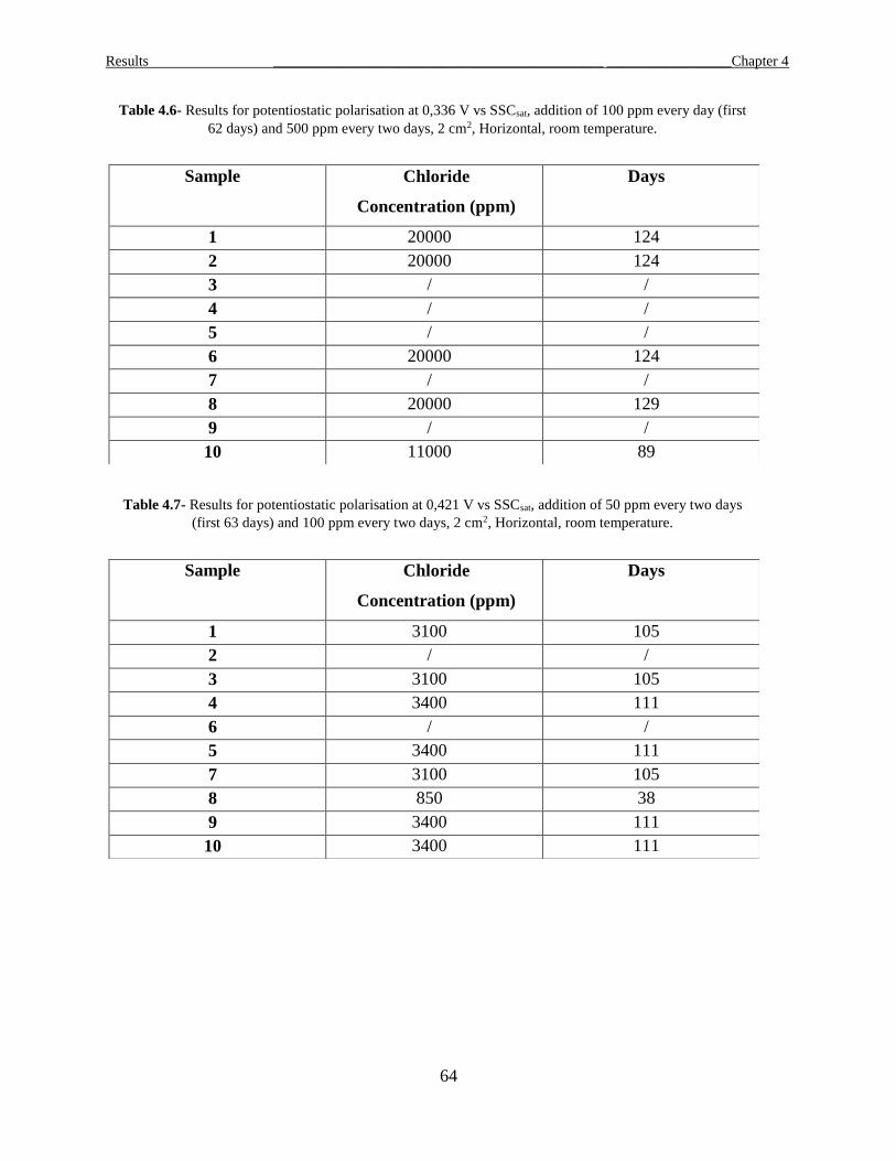
Results _____________________________________________ _________________Chapter 4
64
Table 4.6- Results for potentiostatic polarisation at 0,336 V vs SSCsat, addition of 100 ppm every day (first
62 days) and 500 ppm every two days, 2 cm2, Horizontal, room temperature.
Sample Chloride
Concentration (ppm)
Days
1 20000 124
2 20000 124
3 / /
4 / /
5 / /
6 20000 124
7 / /
8 20000 129
9 / /
10 11000 89
Table 4.7- Results for potentiostatic polarisation at 0,421 V vs SSCsat, addition of 50 ppm every two days
(first 63 days) and 100 ppm every two days, 2 cm2, Horizontal, room temperature.
Sample Chloride
Concentration (ppm)
Days
1 3100 105
2 / /
3 3100 105
4 3400 111
6 / /
5 3400 111
7 3100 105
8 850 38
9 3400 111
10 3400 111

Results _____________________________________________ _________________Chapter 4
65
Figure 4.10 - Results for potentiostatic polarisation at 0,42 V vs Ag/AgCl/KClsat
Figure 4.11- Results for potentiostatic polarisation at 0,335 V vs Ag/AgCl/KClsat

66
Chapter 5
DISCUSSION
Comparison between the results obtained during the thesis work and the literature review will be
conducted in this chapter. The aim of this discussion is to obtain the Pedeferri diagram, discussing
how different electrochemical methods used affect the final drawing of it.
5.1 POTENTIODYNAMIC POLARISATION TEST
The first electrochemical method that is discussed is the potentiodynamic polarisation tests and
how the chloride concentration and setup variable influenced the results of this test.
5.1.1 EFFECT OF CHLORIDE CONCENTRATIONS
As shown in the figures of the previous chapter (Fig. 4.1 to Fig. 4.8), the test conducted are
presented in the forms of potentiodynamic polarisation curves. In those curves, one can distinct
three points, as explained in Chapter 1: the corrosion potential, the pitting or breakdown potential
and the repassivation potential.
Many authors confirm this trend, that to an increase of chlorides, or more in general halides, a
decrease of breakdown potential follows [3, 4], and as expected also in this work this trend is
confirmed.
In order to compare the results obtained with different chloride concentration, a data distribution
of the results have been studied and plotted (Fig 5.1) for specimen with 2 cm2 and at a scan rate of
600 mV/h. In addition, data from previous thesis work are taken into account, for a total of six sets
of test considered, ranging from 100 ppm to 19000 ppm chloride concentration. To build this
integral probability curves it has been taken the whole pool of data of a single set and to each value
a percentage of failure have been attributed: for example, for the test of 1000ppm chloride (Fig.
5.1c), the value 500mV vs Ag/AgCl/KClsat has been attributed the 80% of failure, meaning that in
the tests carried out in this thesis 80% of the specimen undergo pitting corrosion at 500mV. Dually
it can be said that a specific percentage of failure has been attributed a polarization potential: taking
the curve for 3000ppm chloride concentration (Fig 5.1d), the potential at which the 50% of the
specimen failed is about 400mV vs Ag/AgCl/KClsat.

67
The same consideration can be done for the re-passivation potential, but instead of failure of the
specimen (pitting attack occurs), the success of the specimen is considered (the re-passivation is
achieved). For this reason, there is a formation of the peculiar funnel shape of the two curve.
For each percentage considered, the difference between the pitting potential and repassivation
potential give an estimated value of the imperfect passivity range; taking the Pedeferri’s diagram
of Chapter 1 (Fig. 1.15) can be seen that the imperfect passivity lays between the two values of
Eloc and Erep.
a)
b)
c)
d)
e)
f)
Figure 5.4- Probability curves for all the concentration tested. a) 100 ppm, b) 300 ppm, c) 1000 ppm, d) 3000 ppm, e) 10000 ppm, f)
19000 ppm [45]for samples of 2 cm2, 600mV/h

68
It can be seen that for the set of 100 ppm and 300 ppm (Fig 5.1a and Fig.5.1b respectively) some
percentage of failure are missing, this is due to the results obtained in those tests. Recalling the
Pourbaix diagram (Chapter 1.2, Figure 1.2) for the oxygen two zones are defined: the oxygen
reduction and oxygen evolution. In Chapter 1.1 it has been point out that at neutral or basic pH the
cathodic reaction is oxygen reduction, so potential where oxygen reduction is not possible are not
consider significant. For this reason the pitting potentials values above 0,68 V vs Ag/AgCl/KClsat
are not considered.
To compare and to place the result in a single plot, two percentage have been considered: 10% and
90%. The first has been chosen because it has been decided as the limit of safety: 10% means that
only 1 specimen out of 10 reached to the localized corrosion and so it is near the imperfect passivity
and it is the first point for which we observed pitting phenomena. The second has been chosen as
the limit for the pitting corrosion: it means that at that potential 9 specimen out of 10 reached to
the localized corrosion and so it is practically sure to be in the pitting corrosion zone. A similar,
but reverse, thought can be done for the re-passivation phenomena: when the 10% of the specimen
reached to the re-passivation, there it is the limit between the perfect and imperfect passivity; when
the 90% of the specimen re-passivate, it is very probable to be in the perfect passivity zone.
Isoprobability curves have been drown taking the 10% and 90% of failure (pitting) and re-
passivation. From these curves can be distinguished the three zones of the Pedeferri’s diagram
(Chapter 1.6, Fig. 1.15): the perfect passivity zone below the 90% of the re-passivation, the
imperfect passivity between the 10% of re-passivation and 10% of pitting, and the pitting corrosion
zone above the 90% of pitting.
Both linear and logarithm plot are shown in Fig 5.2 and Fig 5.3.
It can be noticed that the linear relationship between the pitting potential and the logarithm of
chloride contents expressed in Chapter 1.5.1 (Eq. 1.14) has been found for both pitting potential
and re-passivation potential. The only discrepancy is for high chloride contents, for which re-
passivation is more difficult

69
Figure 5.2- Isoprobability curves for all the concentration tested ranging from 100ppm to 19000ppm
Figure 5.3- Isoprobability curves in semi-logarithm scale for all the concentration tested: ranging from 100ppm
to 19000ppm
In high concentrations (19000 ppm), it was difficult to attain re-passivation potential points for
90% of the specimen that attained localized corrosion due to the fact that at high concentration
most of the time the specimens suffer a very severe localised corrosion and they are not able to
repassivated if not at very low polarization potential (lower than -200 mV vs Ag/AgCl/KClsat).

70
For sake of completeness, a statistical study has been conducted, measuring the average values,
the standard deviations and the dispersion index of the data. Although the average value of
breakdown potential and repassivation potential do not give a complete understanding of the
phenomenon, being localized corrosion stochastic by nature, they are needed for the definition of
dispersion index value. The dispersion index is the ratio between the standard deviation of a set of
value and the average of the same set [46].
Both standard deviations and dispersion index define the replicability of the test conducted: the
lower is the value of these two, the more probable it is to obtain results similar of the ones obtained
in previous tests.
Before the calculation of the above mentioned statistical number, another quantity has been
introduced: the interval of passivity, which is defined as the difference between the corrosion
potential and the pitting potential.
The average and standard deviation of the pitting potential and repassivation potential are shown
in Table 5.1, while in Table 5.2 the average, standard deviation and dispersion index of the interval
of passivity are calculated.
Table 5.1- Average values and standard deviation of breakdown potentials (Eloc) and repassivation potential (Erep)
Cl- (ppm) Eloc
(V vs SSC)
Average
Erep
(V vs SSC)
Average
Standard Deviation
Eloc V
Standard Deviation
Erep V
100 0,643 0,095 0,085 0,064
300 0,576 0,056 0,073 0,053
1000 0,462 0,035 0,043 0,061
3000 0,408 0,030 0,085 0,064
10000 0,405 -0,027 0,042 0,035
19000 0,405 -0,159 0,017 0,101
Table 5.2- Average values, standard deviations and dispersion indexes (DI) of the interval of passivity(Eloc-
Ecorr)
Cl-
(ppm)
Eloc-Ecorr (V)
Average
Standard
Deviation
Eloc-Ecorr (V)
DI
Eloc-Ecorr
(%)
100 0,644 0,096 14,9
300 0,582 0,083 14,2
1000 0,483 0,072 15.0
3000 0,450 0,037 8,2
10000 0,434 0,057 13,2
19000 0,408 0,025 6,1

71
As can be seen both values of standard deviation and dispersion index show us the stochastic aspect
of localised corrosion: it is easy to deduct it by the values of dispersion index, 4 set of tests out of
6 have a volatility above 10% and only one it’s near 5%, that it is consider a good replicability.
The sets of tests done at 3000 ppm and 19000 ppm have a much lower volatility value than the
others. For 19000 ppm the explanation can be that the chloride contents becomes the predominant
factors for the break of the passivity (the dependence on pH and temperature are lower), while for
other results a minimal and/or variation of pH or temperature scatter influenced more the results;
while for 3000ppm no explanation can be given.
5.1.2 EFFECT OF SURFACE AREA
In order to evaluate the effect of the surface area, specimens with different surface areas (1, 2, 4,
10 and 50 cm2) were selected.
The results of the test conducted are shown in Fig 5.4, with the criterion of failure probability
mentioned above.
Even if a dependence on the exposed area is expected (Fig 5.5), no trend is found in this work.
Figure 5.3- Isoprobability curves of different surface area
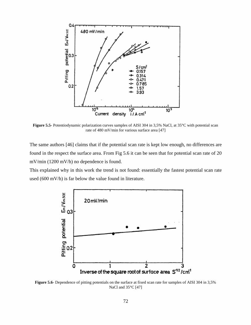
72
Figure 5.5- Potentiodynamic polarization curves samples of AISI 304 in 3,5% NaCl, at 35°C with potential scan
rate of 480 mV/min for various surface area [47]
The same authors [46] claims that if the potential scan rate is kept low enough, no differences are
found in the respect the surface area. From Fig 5.6 it can be seen that for potential scan rate of 20
mV/min (1200 mV/h) no dependence is found.
This explained why in this work the trend is not found: essentially the fastest potential scan rate
used (600 mV/h) is far below the value found in literature.
Figure 5.6- Dependence of pitting potentials on the surface at fixed scan rate for samples of AISI 304 in 3,5%
NaCl and 35°C [47]

73
5.1.3 EFFECT OF POTENTIAL SCAN RATE
The scan rate taken into account in this work range from 1 mV/h to 600mV/h, which is the potential
scan rate imposed by the standard, so from a very fast potentiodynamic polarization to a very slow
potentiodynamic.
The tests have been run with three different concentration: 1000ppm, 3000ppm and 10000ppm.
For the first, three potential scan rate (1 mV/h, 10 mV/h, 600 mV/h) have been used, while for the
chloride concentration have been used or only the continuous potentiodynamic polarization (10
mV/h, 100 mV/h, 600 mV/h for 3000ppm) or only the fastest and slowest (1 mV/h and 600 mV/h
for 10000).
From Fig 5.7 to Fig 5.9 it is shown the effect of the various scan rate, with all the data. Some values
have been removed because above the oxygen evolution threshold.
Figure 5.7 – Pitting potentials at 1000ppm with three different potential scan rate (1mV/h [45], 10mV/h and 600 mV/h)

74
Figure 5.8 - Pitting potentials at 3000ppm with three different potential scan rate (10 mV/h, 100 mV/h, 600 mV/h)
Figure 5.9 - Pitting potentials at 10000ppm with two different potential scan rate (1 mV/h and 600 mV/h [45])
A scan rate dependence is expected: lowering the scan rate, at lower polarization potential the
pitting occur.
It can be clearly seen in Fig 5.7 and Fig 5.9, where pitting potentials value are lower as the potential
scan rate lowers.
For 10000ppm the inverse is observed, no explanation can be given for that phenomenon.
5.2 POTENTIOSTATIC POLARISATION TESTS
The potentiostatic test the aim was to find the critical chloride concentration.
Based he result obtained in the work, only 5 out of 10 reached to the localised corrosion in the test
of 0,335 V vs Ag/AgCl/KClsat, and 4 of them reached the corrosion at 20000ppm chloride. Even
if the breakdown is reached at a very high concentration, this results do not go against the results
obtain with the potentiodynamic, since a pitting potential of 0,42V vs Ag/AgCl/KClsat can be seen
also at high concentration. Fig 5.10 and Fig 5.11 show the percentage of specimens corroded in
function of the chloride in the solution.

75
Figure 5.10- Percentage of corroded specimen in function of the chloride content for the potentiostatic
polarization at 0,335 V vs Ag/AgCl/KClsat
Figure 5.11- - Percentage of corroded specimen in function of the chloride content for the potentiostatic
polarization at 0,420 V vs Ag/AgCl/KClsat
It can be seen from both figures that the specimen suffered the localized attack much beyond the
limit expected from the potentiodynamic. This is due to the form of the Pedeferri’s diagram (Fig
5.8): the critical chloride contents for a specific polarization potential is spread in an order of

76
magnitude more or less, so at that specific polarization potential the pitting can occur at a very
varying chloride contents.
Figure 5.10- Critical chloride concentration for three different polarization potentials
For the other set of potentiostatic tests instead the polarisation potential was very similar to the one
of the previous potentiostatic test (0,41 V vs SSC) and the result are similar to that experiment.
5.3 PEDEFERRI DIAGRAM
Fig. 5.11 show the comparison between all the potentiodynamic and potentiostatic polarization
tests. It can be seen that the results give approximately the same range of values, with the difference
that the potentiostatic give horizontal results (critical chloride contents) while the potentiostatic
give vertical results (pitting potential).

77
Figure 5.11 - Comparison between all the tests conducted in this thesis and the previous one
The results of 1 cm2, 2 cm2, 4 cm2 for 1000 ppm chloride content and the one of 2 cm2 with 10000
ppm chloride content are taken from a previous thesis work [45] and the results of 2 cm2 with
19000 ppm chloride content from an in progress bachelor thesis [48].
So there are two possible way to obtain Pedeferri diagram: using potentiostatic tests to find which
is the critical amount of chloride content for a specific polarisation potential or potentiodynamic
test to find which is the breakdown potential, and repassivation potential, for a specific chloride
concentration. Being the potentiodynamic faster than potentiostatic and giving a similar range of
values, as said earlier, potentiodynamic tests have been chose to get both faster and reliable result.
To plot a Pedeferri’s diagram for AISI 304 stainless steel (Fig 5.8), from all the potentiodynamic
tests, the ones with samples of 2cm2 and with a potential scan rate of 600 mV/h has been chosen
to have uniformity in the data.
As can be seen one can distinguish the three area discussed in chapter one:
The perfect passivity zone, where the potential is less than the last repassivation potential
The imperfect passivity zone, where the potential is between the highest repassivation
potential and the lowest breakdown potential
The corrosion potential, where the potential is higher than the highest breackdown
potential measured
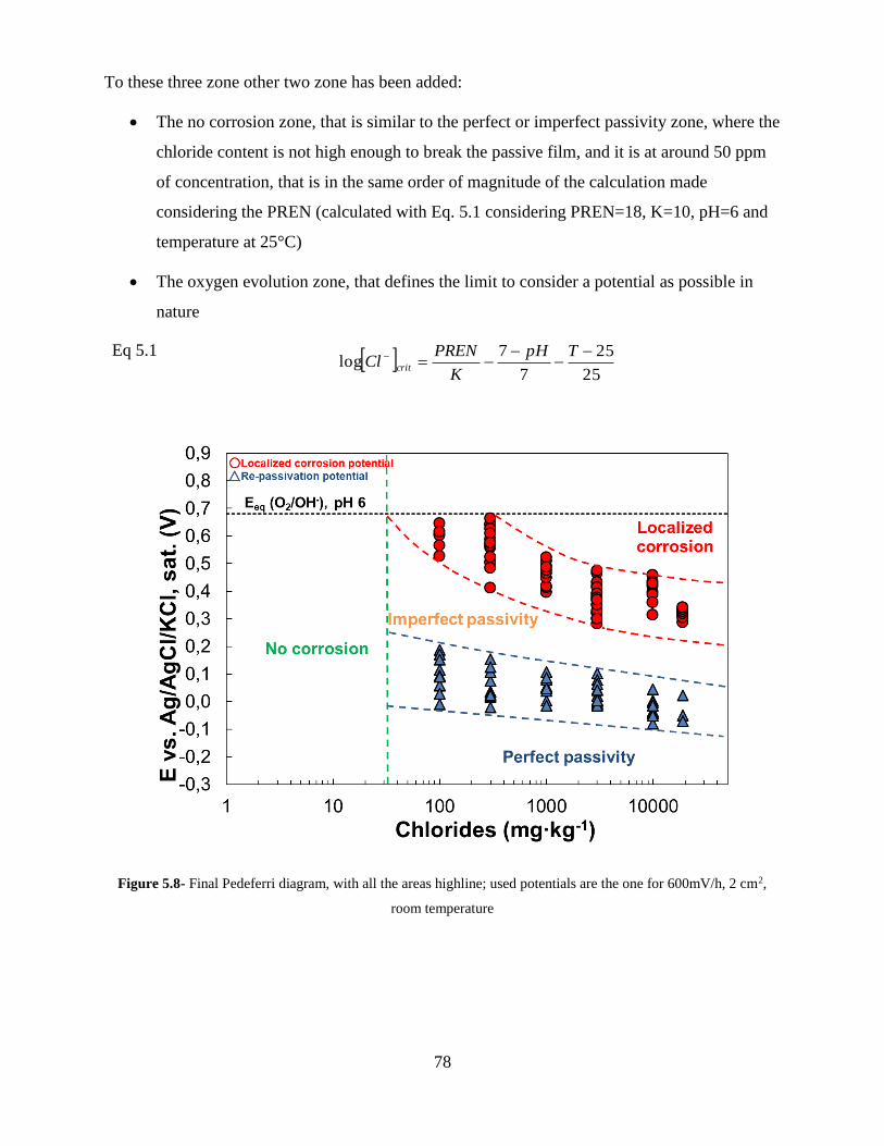
78
To these three zone other two zone has been added:
The no corrosion zone, that is similar to the perfect or imperfect passivity zone, where the
chloride content is not high enough to break the passive film, and it is at around 50 ppm
of concentration, that is in the same order of magnitude of the calculation made
considering the PREN (calculated with Eq. 5.1 considering PREN=18, K=10, pH=6 and
temperature at 25°C)
The oxygen evolution zone, that defines the limit to consider a potential as possible in
nature
Eq 5.1 25
25
7
7log
TpH
K
PRENCl crit
Figure 5.8- Final Pedeferri diagram, with all the areas highline; used potentials are the one for 600mV/h, 2 cm2,
room temperature

79
CONCLUSIONS
In this thesis, potentiodynamic and potentiostatic anodic polarization tests were carried out on
austenitic UNS 304000 stainless steel in order to define the most proper test method for the
definition of Pedeferri diagram. Potentiodynamic tests were performed in the presence of different
chlorides concentration (from 100 to 20,000 mg/kg) and potential scan rates (10 mV/h, 100 mV/h,
600 mV/h) in aerated and neutral solution. Then, potentiostatic tests were carried out at tailored
polarization potential value in order to compare the two methods.
The results of potentiodynamic tests show that:
1. As expected, localized corrosion potential depends on the chlorides content in solution; the
potential varies linearly with the logarithm of chlorides concentration as reported in several
papers and books of the last 40 years
2. Localized corrosion potential and its distribution depends on the potential scan rate:
generally, the localized corrosion potential increases as the scan rate increases, but this
trend was not observed in same of the experimental conditions. This behaviour can be
attributed to the kinetic of localized corrosion initiation, which is not instantaneous: the
localized corrosion potential corresponds to the potential at which the incubation period of
corrosion and the kinetic of the test method are comparable. The distribution (deviation) of
localized corrosion potential values depends on potential scan rate and increases as the scan
rate decreases. As a possible interpretation, longer test times can affect the electrochemical
behaviour of the metal, in particular the properties of the passive film, as its thickness. In
other words, longer tests (i.e. low potential scan rate) can induce modification (anodizing)
of the passive oxide with the consequent modification of its corrosion resistance during the
test;
3. From point 2 it is possible to conclude that low scan rate would be preferable because they
provide lower localized corrosion potential (more conservative approach) but at the same
times the dispersion of data is generally larger;
4. The potentiodynamic polarization method (continuous scan or stepwise) affects also the
localized corrosion potential distribution: in the presence of a stepwise polarization, the
data dispersion increases.

80
The performed potentiostatic tests showed that the two test methods are comparable, and a large
deviation from the mean value is observed also for potentiostatic test. In principle, potentiostatic
polarization test seems preferable because approach to the real condition where the oxidizing
power of the electrolyte in contact with the metal is fixed (oxygen reduction process) while
potentiodynamic test is strongly accelerated and does not simulate any practical condition. As
already said.
A first attempt to draw the Pedeferri diagram UNS 304000 stainless st.eel in near neutral pH and
at room temperature has been carried out. The results are promising even if the selection of the
best tests method is ongoing.

81
BIBLIOGRAPHY
[1] L. Bertolini, B. Elsener, P. Pedeferri, E. Redaelli, R.B. Polder, “Corrosion of steel in concrete:
Prevention, Diagnosis, Repair”; 2nd Edition; Wiley-VCH Verlag GmbH, 2013
[2] L. Lazzari, “9.1: Aspetti generali della corrosion”, Enciclopedia degli Idrocarburi, Volume 5,
Treccani – ENI, 2008
[3] E. McCafferty, “Introduction to corrosion science”, New York: Seacus, New Jersey, USA;
Sprinfer Verlag, 2010
[4] Z. Szklarska Smialowska, “Pitting Corrosion of Metals”, National Assn of Corrosion
Engineers, 1986
[5] A. Pardo, E. Otero, M.C. Merino, M.D. Lopez, M.V. Utrilla, F. Moreno, “Influence of pH and
Chloride Concentration on the pitting and crevice corrosion behaviour of Hig-Alloy stainless
steels”, Corrosion Engeineerig Section
[6] H. Strehblow, “Nucleation and repassivation of corrosion pits for pitting on iron and nickel”;
Materials and corrosion/Werkstoffe und Korrosion, 27 (11), 1976, pp 792-799
[7] N. Sridhar, “The role of local Chemistry Changes in the Repassivation of Localized Corrosion
– a review”, NACE International, Corrosion Conference&Expo 2016, paper no. 7083
[8] Sharp, La Liberte, “The propagation of Crevice Corrosion in Aloys Being considered for cleach
plant service”, Corrosion/78, Preprint No. 16, National Associatioon of Corrosion Engineers,
Huoston, Texas, 1978
[9] L. Lazzari, P. Pedeferri, “Cathodic Protection”, Milano, Polipress, 2006
[10] K.V.S. Ramana, T. Anita, S. Mandal, S. Kaliappan, H. Shaikh, P.V. Sivaprasad, R.K. Dayal,
H.S. Khatak, “Effect of different environmental parameters on pitting behavior of AISI type
316L Stainless Steel: Experimental Studies and Neural Network Modeling”,
Materials&Design, Volume 30, 3770-3775, 2009
[11] C.O.A. Olsson, D. Landolt, “Passive films on stainless steels – chemistry, structure and
growth”, Electrochimica Acta, Volume 48, 1093-1104, 2003.
[12] A. Pardo, M.C. Merino, A.E. Coy, F. Viejo, R. Arrabal, E. Matykina, “Effect of Mo and Mn
addition on the corrosion behaviour of AISI 304 and 316 stainless steels in H2SO4”,
Corrosion Science, Volume 50, 780-794, 2008
[13] A.J. Sedricks, “Corrosion of stainless steels”, 1st Edition, New York, John Wiley&Sons, 1975
[14] A. Pardo, M.C. Merino, A.E. Coy, F. Viejo, R. Arrabal, E. Matykina, “Pitting behaviour of
austenitic stainless steels – combining effect on Mn and Mo additions”, Corrosion Science,
Volume 50, 1796-1806, 208
[15] I. Olefjord, L. Wegrelius, “The influence of nitrogen on the passivation of stainless steel”,
Corrosion Science, Volume 38, 1203-1220, 1996.
[16] H.Baba, T. Kodama, Y. Katada, “Role of nitrogen on the corrosion behaviour of austenitic
stainless steels”, Corrosion Science, Volume 44, 2393-2407, 2002
[17] U.K. Mudali, R.K Dayal, J.B. Gnanamoorthy, P. Rodriguez, “High nitrogen steels:
relationship between pitting and intergranular corrosion of nitrogen-bearing austenitic
stainless steels”, ISIJ International, Volume 36, 799-806, 1996
[18] M.A. Baker, J.E. Castle, “The initiation of pitting corrosion at MnS inclusions”, Corrosion
Science, Volume 34, 667-682, 1993

82
[19] P. Schmuki, H. Hildebrand, A. Friedrich, S. Virtanen, “The composition of the boundary
region of MnS inclusions in stainless steel and its relevance in triggering pitting corrosion”,
Corroson Science, Volume 47, 1239-1250, 2005
[20] L. Peguet, B. Malki, B. Baroux, “Influence of cold working on ptting corrosion of stainless
steels”, Corrosion Science, Volume 49, 1933-1948, 2007
[21] A.C. de Oliveira, M.C.L. de Oliveira, C.T.Rios, R.A. Antunes, “The effect of mechanical
polishing and finishing on the corrosion resistance of AISI 304 stainless steel”, Corrosion
Engineering, Science and Technology, Volume 51, 416-428, 2016
[22] H.R. Bakhsheshi-Rad, B. Haerian, A. Najafizadeh, M.H. Idris, M.R.A. Kadir, E. Hamzah, M.
Daroonparvar,, “Cold deformation and heat treatment influence on the microstructures and
corrosion behaviour of AISI 304 stainless steel”, Canadian Metallurgical Quarterly, Volume
52:4, 449-457, 2013.
[23] H.S Lee, D.S. Kim, J.S. Jung, Y.S. Pyoun, K. Shin, “Influence of peening on the corrosion
properties of AISI 304 stainless steel”, Canadian Metallurgical Quarterly, Volume 52:4, 449-
457, 2013.
[24] H.P. Leckie, H.H. Uhlig, “ Environmental factors affecting the critical potential for pitting in
18-8 stainless steel”, Journal of the Electrochemical Society, Volume 113, 1262, 1966
[25] D.H. Hur, Y.S. Park, “Effect of temperature on the pitting behaviour and passive film
characteristics of Alloy 600 in chloride solution”, NACE International, Volume 62, 2006.
[26] M.V. Cardoso, S.T. Amaral, E.M.A. Martini, “Temperature effect in the corrosion resistance
of Ni-Fe-Cr alloy in chloride medium”, Corrosion Science, Volume 50, 2529-2436, 2008
[27] B.R. Tzaneva, “Effect of pH on the corrosion behavior of high nitrogen stainless steel in
chloride medium”, Journal of Chemical Technology and Metallurgy, Volume 48, 383-390,
2013.
[28] K.V.S. Ramana, T. Anita, S. Mandal, S. Kaliappan, H. Shaikh, P.V. Sivaprasad, R.K. Dayal,
H.S. Khatak, “Effect of different environmental parameters on pitting behaviour of AISI type
316L Stainless Steel: Experimental Studies and Neural Network Modelling”,
Materials&Design, Volume 30, 3770-3775, 2009.
[29] A.U. Malik, P.C. Mayan Kutty, N.A. Siddiqi, I.N. Andijiani, S. Ahmed, “The influence of pH
and chloride concentration on the corrosion behaviour of AISI 316L steel in aqueous
solutions”, Corrosion Science, Volume 33, 1809-1827, 1992
[30] L. Freire, M.J. Carmezima,c, M.G.S. Ferreira,, M.F. Montemora, “The electrochemical
behaviour of stainless steel AISI 304 in alkaline solutions with different pH in the presence
of chlorides”, Electrochimica Acta, Volume 56, 5280–5289, 2011.
[31] E.C. Hornus, M.A. Rodríguez, R.M. Carranza, R.B. Rebak, “Effect of Temperature and
Chloride Concentration on the Crevice Corrosion Resistance of Austenitic Stainless Steels”,
NACE 2016, Paper No.7170, 2016
[32] N.G. Thompson, B.C Syrett, “Relationship between conventional pitting and protection
potential and a new, unique pitting potential”, Corrosion, Volume 48, 649-659, 1992
[33] R. Baboian, G.S. Haynes, ”Cyclic polarization measurements-Experimental procedures and
evaluation of test data”, Electrochemical Corrosion Testing, ASTM STP727, 274-282, 1981
[34] H.P. Leckie, “A contribution to the applicability of critical pitting potentials”, Journal of
electrochemical society, Volume 117, 1152-1153, 1970
[35] W. Schwenk, “Theory of stainless steel pitting”, Corrosion, Volume 20, 129-137, 1964
[36] Yi, Cho, Al Zaabi, Addad, Jang; “Potentiodynamic polarization behaviour of AISI type 316
stainless steel in NaCl solution”, Corrosion Science, Volume 74, 92-97, 2013

83
[37] Tian, Li, Du, Chen, Wu, “Effects of applied potential on stable pitting of 304 stainless steel”,
Corrosion Science, Volume 93, 242-255, 2015
[38] A. Celant, “Pedeferri diagrams of AISI 304 and AISI 316 stainless steels: effect of the
chlorides on pitting and repassivation potentials”, Master Thesis, Academic year 2014-2015
[39] Alonso-Falleiros, Hakim, Wolync, “Comparison between potentiodynamic and potentiostatic
tests or pitting potential measurements of duplex stainless steels”, Corrosion Science,
Volume 55, 443-448, 1999
[40] A. Broli, H. Holtan, “Determination of characteristic pitting potentials for aluminium by use
of potentiostatic methods”, Corrosion Science, Volume 17, 59-69,1977
[41] S. Frangini, N. De Cristofaro, “Analysis of galvanostatic polarization method for determining
reliable pitting potentials on stainless steels in crevice-free conditions”, Corrosion Science,
Volume 45, 2769-2786, 2003
[42] L.A. Ellingstone, T.J. Shedlosky, G.P Bierwagen, E.R de la Rie, L.B. Brostoff, “Use of
electrochemical impedance spectroscopy in the evaluation of coating for outdoor bronze”,
Studies in Conservation, Volume 49, 2004, 53-62, 2004
[43] X. Zhang, D. Loveday, A. Krebs, “Application of electrochemical techniques in the corrosion
process of rebar in concrete (I)”, NACE international, Corrosion Conference and EXPO
2015, Paper No. 5481, 2015
[44] G. Contreras, P. Fassina, G. Fumagalli, S. Goidanich, L. Lazzari, E. Mazzola, “A study on
metastability phenomena of passive films for corrosion resistant alloys”, Electrochimica
Acta, 52 (2007) 7577–7584
[45] A. Rao; “Comparison of potentiodynamic and potentiostatic polarization tests for the
determination of the pedeferri’s diagram of stainless steels”; Master thesis, Politecnico di
Milano, 2017
[46] D.G. Kleinbaum, L.L. Kupper, A. Nizam, K.E. Muller, “Applied regression analysis and other
multivariable methods”, 4th Edition, Brooks/Cole, 2008
[47] Toshio Shibata, “Surface area dependence of pitting potential”, Corrosion Engineering,
Volume 31, 643-649, 1982
[48] L. Soffientini, Bachelor thesis, in progress

84