Embed Size (px)
Citation preview
Ethiopian TVET-System
Electro Mechanical Equipment
Maintenance Supervision
Level IV
Based on March, 2017G.C. Occupational Standard
Module Title: Apply Principles of Hydraulics to Pipe
and Channel Flow
TTLM Code: EIS EES4 TTLM 0820 v1
Aug, 2020
Electro mechanical Equipment maintenance supervision
Level-IV
Author/Copyright: Federal TVET Agency Version -1 Aug. 2020
Page 2 of 117
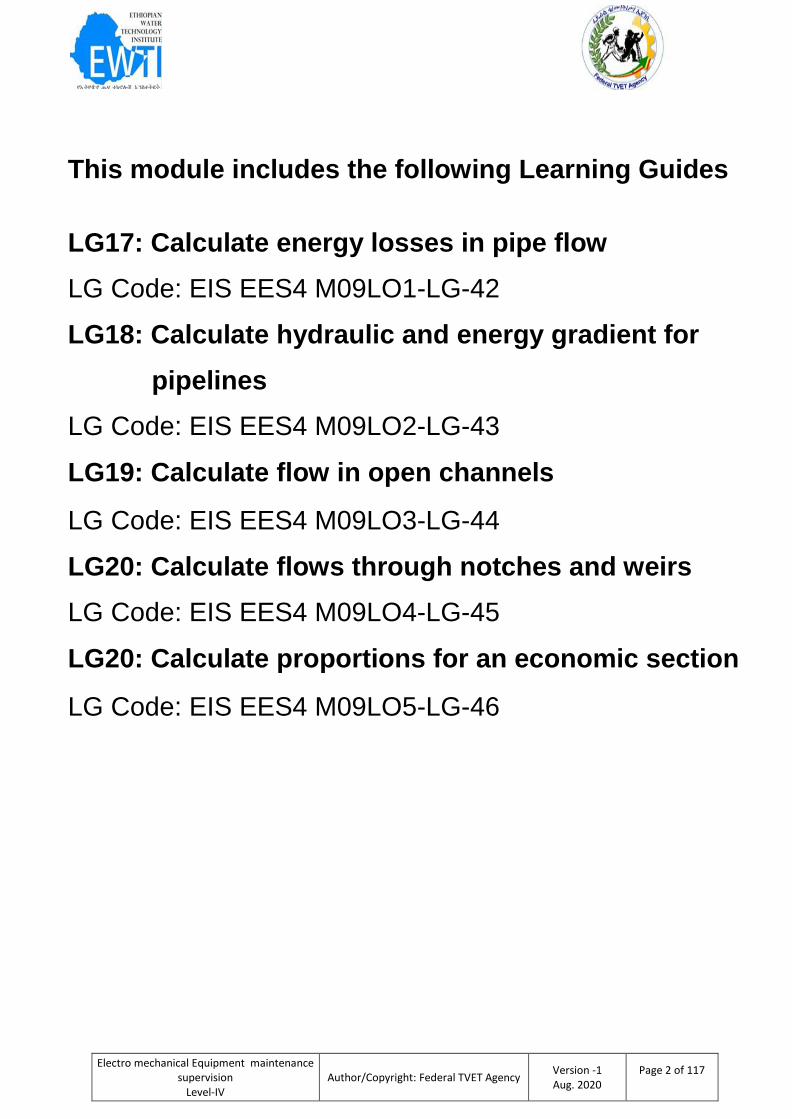
This module includes the following Learning Guides
LG17: Calculate energy losses in pipe flow
LG Code: EIS EES4 M09LO1-LG-42
LG18: Calculate hydraulic and energy gradient for
pipelines
LG Code: EIS EES4 M09LO2-LG-43
LG19: Calculate flow in open channels
LG Code: EIS EES4 M09LO3-LG-44
LG20: Calculate flows through notches and weirs
LG Code: EIS EES4 M09LO4-LG-45
LG20: Calculate proportions for an economic section
LG Code: EIS EES4 M09LO5-LG-46
Electro mechanical Equipment maintenance supervision
Level-IV
Author/Copyright: Federal TVET Agency Version -1 Aug. 2020
Page 3 of 117
This learning guide is developed to provide you the necessary information regarding the
following content coverage and topics:
Energy losses in pipe flow
hydraulic Measurements
Applying hydraulic software
Identifying inconsistent data on flow conditions.
This guide will also assist you to attain the learning outcome stated in the cover page.
Specifically, upon completion of this Learning Guide, you will be able to:
.Measurements are reviewed and compared against expected trends.
Standard processes and software are used to check, edit, verify and audit data.
Standard processes are used to identify, estimate, adjust and justify data and review inconsistent data on flow conditions.
Records are prepared in a format suitable for dissemination
Learning Instructions:
1. Read the specific objectives of this Learning Guide.
2. Follow the instructions described below
3. Read the information written in the “Information Sheets 1- 4”. Try to understand what are
being discussed.
4. Accomplish the “Self-checks1,2,3 and 4 ” in each information sheets on pages
16,21,31and 34.
5. Ask from your teacher the key to correction (key answers) or you can request your
teacher to correct your work. (You are to get the key answer only after you finished
answering the Self-checks).
6. After You accomplish self check, ensure you have a formative assessment and get a
satisfactory result; then proceed to the next LG.
Instruction Sheet Learning Guide 42: Calculate energy losses
in pipe flow
Electro mechanical Equipment maintenance supervision
Level-IV
Author/Copyright: Federal TVET Agency Version -1 Aug. 2020
Page 4 of 117
Information Sheet-1 Energy losses in pipe flow
Introduction
The total energy loss in a pipe system is the sum of the major and minor losses. Major losses are
associated with frictional energy loss that is caused by the viscous effects of the fluid and roughness of
the pipe wall. Major losses create a pressure drop along the pipe since the pressure must work to
overcome the frictional resistance. The Darcy-Weisbach equation is the most widely accepted formula
for determining the energy loss in pipe flow. In this equation, the friction factor (f ), a dimensionless
quantity, is used to describe the friction loss in a pipe. In laminar flows, f is only a function of the
Reynolds number and is independent of the surface roughness of the pipe. In fully turbulent flows, f
depends on both the Reynolds number and relative roughness of the pipe wall.
1.1 Calculating energy losses in pipe flows
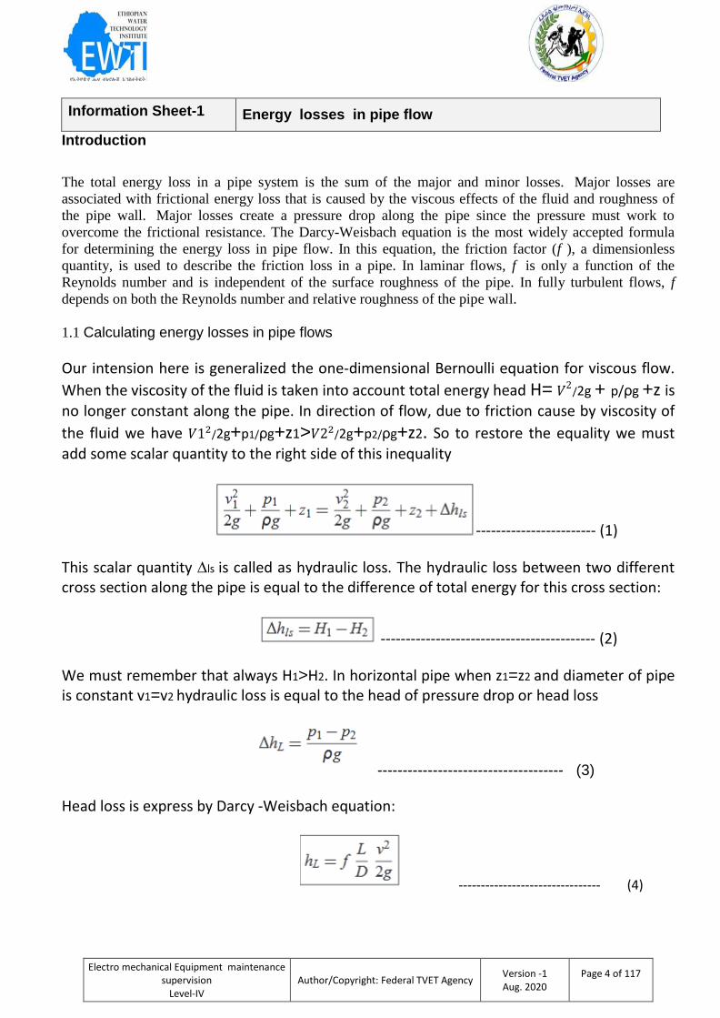
Our intension here is generalized the one-dimensional Bernoulli equation for viscous flow.
When the viscosity of the fluid is taken into account total energy head H= 𝑉2/2g + p/ρg +z is
no longer constant along the pipe. In direction of flow, due to friction cause by viscosity of
the fluid we have 𝑉12/2g+p1/ρg+z1>𝑉22/2g+p2/ρg+z2. So to restore the equality we must
add some scalar quantity to the right side of this inequality
------------------------ (1)
This scalar quantity ∆ls is called as hydraulic loss. The hydraulic loss between two different cross section along the pipe is equal to the difference of total energy for this cross section:
------------------------------------------- (2)
We must remember that always H1>H2. In horizontal pipe when z1=z2 and diameter of pipe is constant v1=v2 hydraulic loss is equal to the head of pressure drop or head loss
------------------------------------- (3)
Head loss is express by Darcy -Weisbach equation:
-------------------------------- (4)
Electro mechanical Equipment maintenance supervision
Level-IV
Author/Copyright: Federal TVET Agency Version -1 Aug. 2020
Page 5 of 117
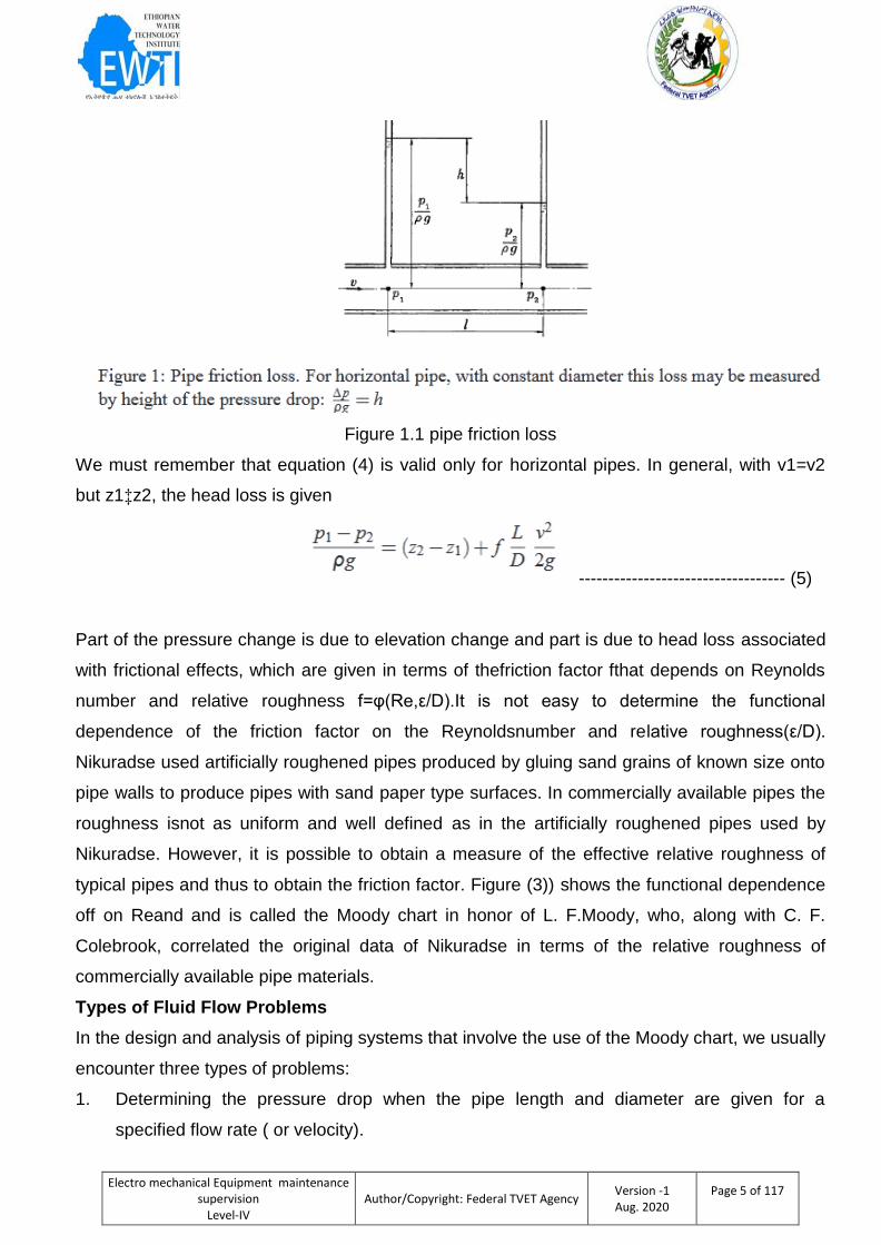
Figure 1.1 pipe friction loss
We must remember that equation (4) is valid only for horizontal pipes. In general, with v1=v2
but z1‡z2, the head loss is given
----------------------------------- (5)
Part of the pressure change is due to elevation change and part is due to head loss associated
with frictional effects, which are given in terms of thefriction factor fthat depends on Reynolds
number and relative roughness f=φ(Re,ε/D).It is not easy to determine the functional
dependence of the friction factor on the Reynoldsnumber and relative roughness(ε/D).
Nikuradse used artificially roughened pipes produced by gluing sand grains of known size onto
pipe walls to produce pipes with sand paper type surfaces. In commercially available pipes the
roughness isnot as uniform and well defined as in the artificially roughened pipes used by
Nikuradse. However, it is possible to obtain a measure of the effective relative roughness of
typical pipes and thus to obtain the friction factor. Figure (3)) shows the functional dependence
off on Reand and is called the Moody chart in honor of L. F.Moody, who, along with C. F.
Colebrook, correlated the original data of Nikuradse in terms of the relative roughness of
commercially available pipe materials.
Types of Fluid Flow Problems
In the design and analysis of piping systems that involve the use of the Moody chart, we usually
encounter three types of problems:
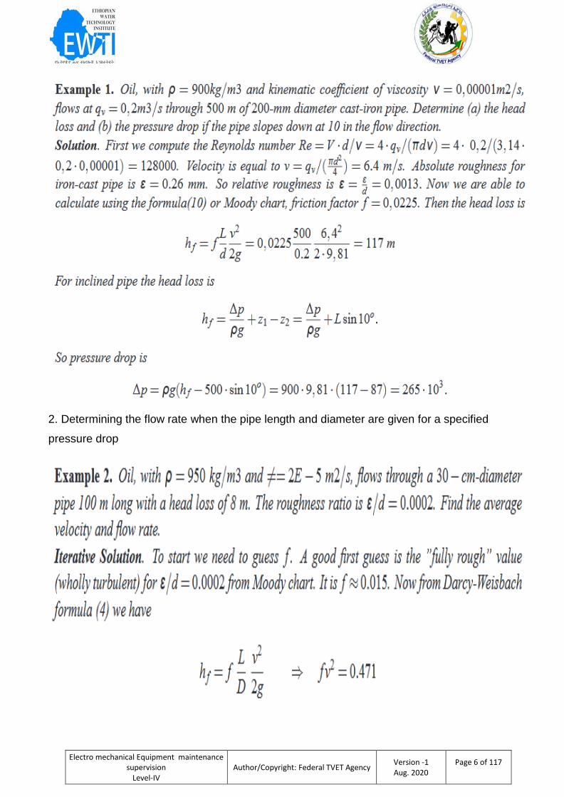
1. Determining the pressure drop when the pipe length and diameter are given for a
specified flow rate ( or velocity).
Electro mechanical Equipment maintenance supervision
Level-IV
Author/Copyright: Federal TVET Agency Version -1 Aug. 2020
Page 6 of 117
2. Determining the flow rate when the pipe length and diameter are given for a specified
pressure drop
Electro mechanical Equipment maintenance supervision
Level-IV
Author/Copyright: Federal TVET Agency Version -1 Aug. 2020
Page 7 of 117
1.1.2. Calculating head losses in non-circular pipes
The basic approach to all piping systems is to write the Bernoulli equation between two points, connected by a streamline, where the conditions are known. For example, between the surface of a reservoir and a pipe outlet.
The total head at point 0 must match with the total head at point 1, adjusted for any increase in head due to pumps, losses due to pipe friction and so-called "minor losses" due to entries, exits, fittings, etc. Pump head developed is generally a function of the flow through the system, with head rise decreasing with increasing flow through the pump.
Friction Losses in Pipes
Friction losses are a complex function of the system geometry, the fluid properties and the flow rate in the system. By observation, the head loss is roughly proportional to the square of the flow rate in most engineering flows (fully developed, turbulent pipe flow). This observation leads to the Darcy-Weisbach equation for head loss due to friction:
which defines the friction factor, f. f is insensitive to moderate changes in the flow and is constant for fully turbulent flow. Thus, it is often useful to estimate the relationship as the head being directly proportional to the square of the flow rate to simplify calculations.
Reynolds Number is the fundamental dimensionless group in viscous flow. Velocity times Length Scale divided by Kinematic Viscosity.
Electro mechanical Equipment maintenance supervision
Level-IV
Author/Copyright: Federal TVET Agency Version -1 Aug. 2020
Page 8 of 117
Relative Roughness relates the height of a typical roughness element to the scale of the flow, represented by the pipe diameter, D.
Pipe Cross-section is important, as deviations from circular cross-section will cause secondary flows that increase the pressure drop. Non-circular pipes and ducts are generally treated by using the hydraulic diameter,
in place of the diameter and treating the pipe as if it were round.
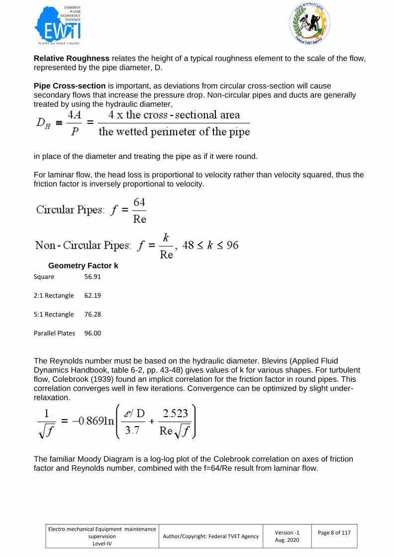
For laminar flow, the head loss is proportional to velocity rather than velocity squared, thus the friction factor is inversely proportional to velocity.
Geometry Factor k
Square 56.91
2:1 Rectangle 62.19
5:1 Rectangle 76.28
Parallel Plates 96.00
The Reynolds number must be based on the hydraulic diameter. Blevins (Applied Fluid Dynamics Handbook, table 6-2, pp. 43-48) gives values of k for various shapes. For turbulent flow, Colebrook (1939) found an implicit correlation for the friction factor in round pipes. This correlation converges well in few iterations. Convergence can be optimized by slight under-relaxation.
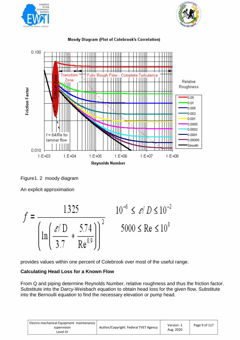
The familiar Moody Diagram is a log-log plot of the Colebrook correlation on axes of friction factor and Reynolds number, combined with the f=64/Re result from laminar flow.
Electro mechanical Equipment maintenance supervision
Level-IV
Author/Copyright: Federal TVET Agency Version -1 Aug. 2020
Page 9 of 117
Figure1. 2 moody diagram
An explicit approximation
provides values within one percent of Colebrook over most of the useful range.
Calculating Head Loss for a Known Flow
From Q and piping determine Reynolds Number, relative roughness and thus the friction factor. Substitute into the Darcy-Weisbach equation to obtain head loss for the given flow. Substitute into the Bernoulli equation to find the necessary elevation or pump head.
Electro mechanical Equipment maintenance supervision
Level-IV
Author/Copyright: Federal TVET Agency Version -1 Aug. 2020
Page 10 of 117
Calculating Flow for a Known Head
Obtain the allowable head loss from the Bernoulli equation, then start by guessing a friction factor. (0.02 is a good guess if you have nothing better.) Calculate the velocity from the Darcy-Weisbach equation. From this velocity and the piping characteristics, calculate Reynolds Number, relative roughness and thus friction factor. Repeat the calculation with the new friction factor until sufficient convergence is obtained. Q = VA.
Minor Losses
Although they often account for a major portion of the head loss, especially in process piping, the additional losses due to entries and exits, fittings and valves are traditionally referred to as minor losses. These losses represent additional energy dissipation in the flow, usually caused by secondary flows induced by curvature or recirculation. The minor losses are any head loss present in addition to the head loss for the same length of straight pipe.
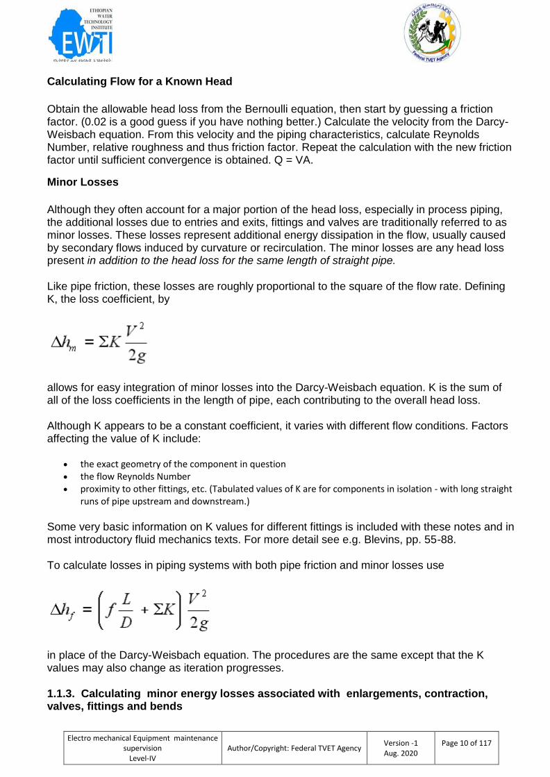
Like pipe friction, these losses are roughly proportional to the square of the flow rate. Defining K, the loss coefficient, by
allows for easy integration of minor losses into the Darcy-Weisbach equation. K is the sum of all of the loss coefficients in the length of pipe, each contributing to the overall head loss.
Although K appears to be a constant coefficient, it varies with different flow conditions. Factors affecting the value of K include:
the exact geometry of the component in question the flow Reynolds Number proximity to other fittings, etc. (Tabulated values of K are for components in isolation - with long straight
runs of pipe upstream and downstream.)
Some very basic information on K values for different fittings is included with these notes and in most introductory fluid mechanics texts. For more detail see e.g. Blevins, pp. 55-88.
To calculate losses in piping systems with both pipe friction and minor losses use
in place of the Darcy-Weisbach equation. The procedures are the same except that the K values may also change as iteration progresses.
1.1.3. Calculating minor energy losses associated with enlargements, contraction, valves, fittings and bends
Electro mechanical Equipment maintenance supervision
Level-IV
Author/Copyright: Federal TVET Agency Version -1 Aug. 2020
Page 11 of 117
Two types of energy loss predominate in fluid flow through a pipe network; major losses, and
minor losses. Major losses are associated with frictional energy loss that is caused by the
viscous effects of the medium and roughness of the pipe wall. Minor losses, on the other hand,
are due to pipe fittings, changes in the flow direction, and changes in the flow area. Due to the
complexity of the piping system and the number of fittings that are used, the head loss
coefficient (K) is empirically derived as a quick means of calculating the minor head losses.
The term “minor losses”, used in many textbooks for head loss across fittings, can be
misleading since these losses can be a large fraction of the total loss in a pipe system. In fact,
in a pipe system with many fittings and valves, the minor losses can be greater than the major
(friction) losses. Thus, an accurate K value for all fittings and valves in a pipe system is
necessary to predict the actual head loss across the pipe system. K values assist engineers in
totaling all of the minor losses by multiplying the sum of the K values by the velocity head to
quickly determine the total head loss due to all fittings. Knowing the K value for each fitting
enables engineers to use the proper fitting when designing an efficient piping system that can
minimize the head loss and maximize the flow rate. Loss coefficient (K) for a range of pipe
fittings, including several bends, a contraction, an enlargement, and a gate valve
The resistance to flow in a pipe network causes loss in the pressure head along the flow. The
overall head loss across a pipe network consists of the following:
Major losses (hmajor), and
Minor losses (hminor)
(i) Major losses Major losses refer to the losses in pressure head of the flow due to
friction effects. Such losses can be evaluated by using the Darcy-Weisbach equation:
where f isthe Darcy friction factor, L is the length of the pipe segment, v is the flow velocity, D is
the diameter of the pipe segment, and g is acceleration due to gravity. Equation (1) is valid for
any fully-developed, steady and incompressible flow.
The friction factor fcan be calculated by the following empirical formula, known as the Blasius
formula, valid for turbulent flow in smooth pipes with ReD< 105:
(ii) Minor losses
Electro mechanical Equipment maintenance supervision
Level-IV
Author/Copyright: Federal TVET Agency Version -1 Aug. 2020
Page 12 of 117
In a pipe network, the presence of pipe fittings such as bends, elbows, valves, sudden
expansion or contraction causes localized loss in pressure head. Such losses are termed as
minor losses. Minor losses are expressed using the following equation:
where Kis called the Loss Coefficient of the pipe fitting under consideration. Minor losses are
also expressed in terms of the equivalent length of a straight pipe (Leq) that would cause the
same head loss as the fitting under consideration:
or
We shall determine the head losses across sudden enlargement, sudden contraction, sharp
bend (90 ° elbow), smooth bend, and a straight section.
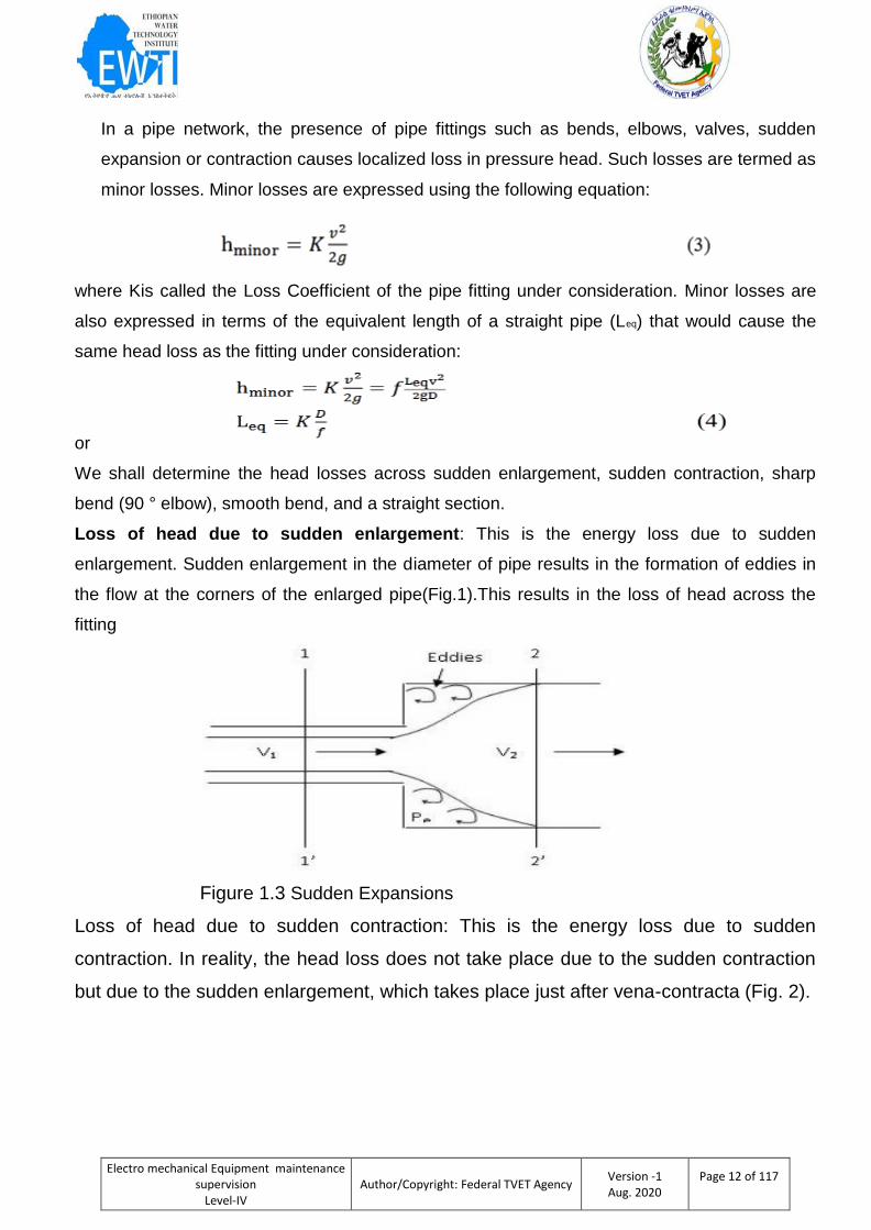
Loss of head due to sudden enlargement: This is the energy loss due to sudden
enlargement. Sudden enlargement in the diameter of pipe results in the formation of eddies in
the flow at the corners of the enlarged pipe(Fig.1).This results in the loss of head across the
fitting
Figure 1.3 Sudden Expansions
Loss of head due to sudden contraction: This is the energy loss due to sudden
contraction. In reality, the head loss does not take place due to the sudden contraction
but due to the sudden enlargement, which takes place just after vena-contracta (Fig. 2).
Electro mechanical Equipment maintenance supervision
Level-IV
Author/Copyright: Federal TVET Agency Version -1 Aug. 2020
Page 13 of 117
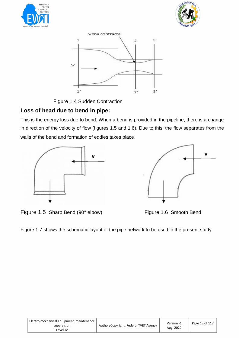
Figure 1.4 Sudden Contraction
Loss of head due to bend in pipe:
This is the energy loss due to bend. When a bend is provided in the pipeline, there is a change
in direction of the velocity of flow (figures 1.5 and 1.6). Due to this, the flow separates from the
walls of the bend and formation of eddies takes place.
Figure 1.5 Sharp Bend (90° elbow) Figure 1.6 Smooth Bend
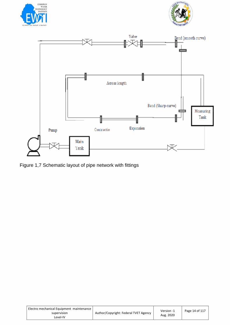
Figure 1.7 shows the schematic layout of the pipe network to be used in the present study
Electro mechanical Equipment maintenance supervision
Level-IV
Author/Copyright: Federal TVET Agency Version -1 Aug. 2020
Page 14 of 117
Figure 1,7 Schematic layout of pipe network with fittings
Electro mechanical Equipment maintenance supervision
Level-IV
Author/Copyright: Federal TVET Agency Version -1 Aug. 2020
Page 15 of 117
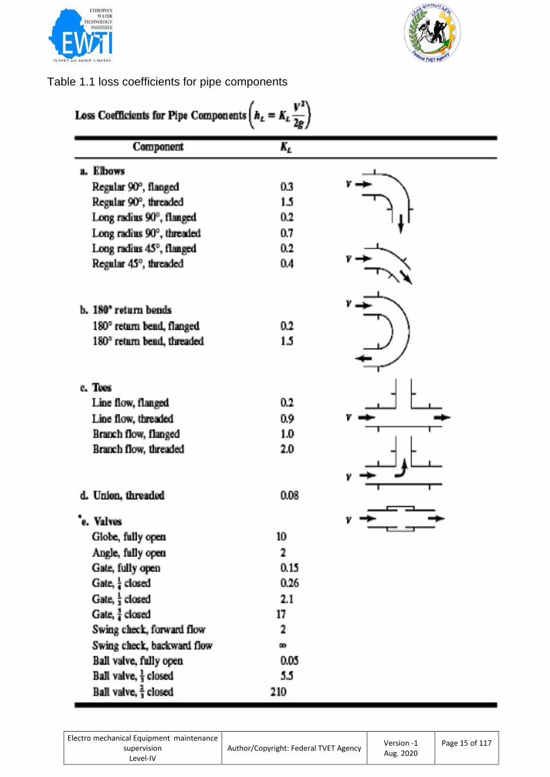
Table 1.1 loss coefficients for pipe components
Electro mechanical Equipment maintenance supervision
Level-IV
Author/Copyright: Federal TVET Agency Version -1 Aug. 2020
Page 16 of 117
Self-Check -1 Written Test
Direction: write the answer for the following questions. Use the Answer sheet provided
1. Determining the pipe diameter when the pipe length and flow rate are given for a
specified pressure drop. Oil, with ρ=950kg/m3and6==2E−5m2/s, flows through
a30−cm-diameterpipe 100 m long with a head loss of 8 m. The roughness ratio is
ε/d=0.0002. Find the average velocity and flow rate.
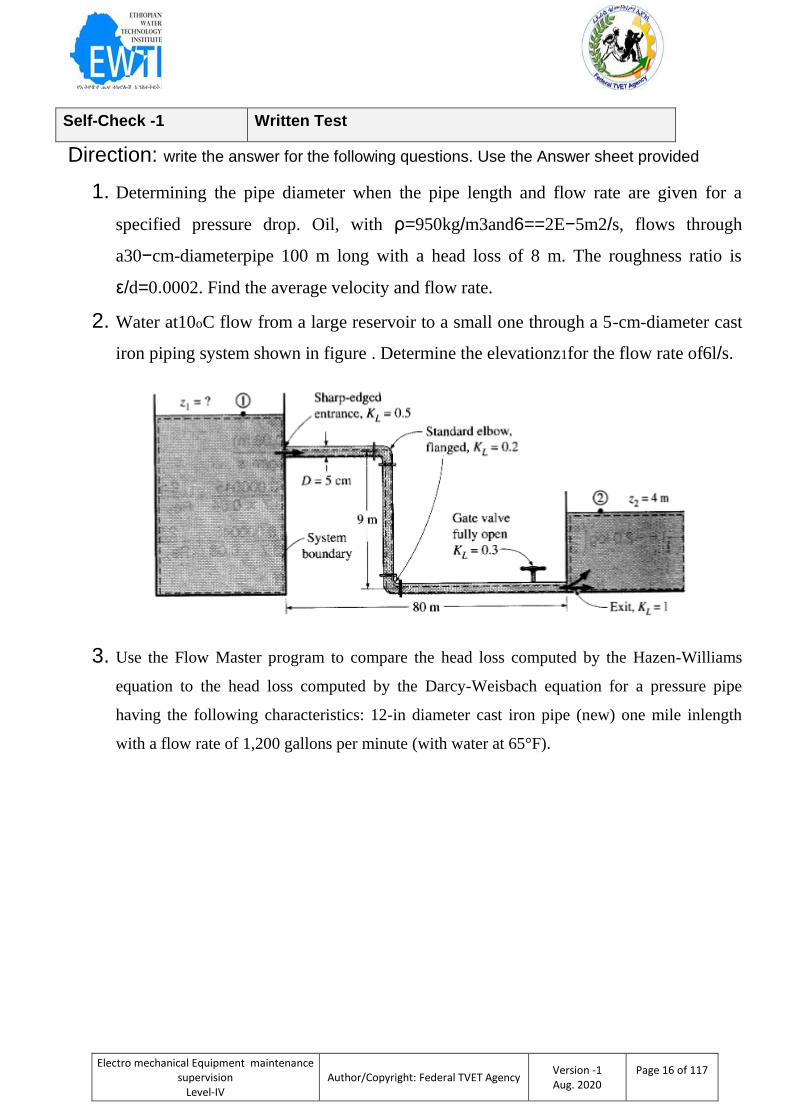
2. Water at10oC flow from a large reservoir to a small one through a 5-cm-diameter cast
iron piping system shown in figure . Determine the elevationz1for the flow rate of6l/s.
3. Use the Flow Master program to compare the head loss computed by the Hazen-Williams
equation to the head loss computed by the Darcy-Weisbach equation for a pressure pipe
having the following characteristics: 12-in diameter cast iron pipe (new) one mile inlength
with a flow rate of 1,200 gallons per minute (with water at 65°F).
Electro mechanical Equipment maintenance supervision
Level-IV
Author/Copyright: Federal TVET Agency Version -1 Aug. 2020
Page 17 of 117
Answer Sheet-1
Name: _________________Date: ______________
Answer
1. ______________________________________________________________________________
______________________________________________________________________________
______________________________________________________________________________
______________________________________________________________________________
______________________________________________________________________________
______________________________________________________________________________
____________________________________________________________________________
2. ______________________________________________________________________________
______________________________________________________________________________
______________________________________________________________________________
______________________________________________________________________________
______________________________________________________________________________
______________________________________________________________________________
______________________________________________________________________________
_______________________________________________________________________
3. ______________________________________________________________________________
______________________________________________________________________________
______________________________________________________________________________
______________________________________________________________________________
______________________________________________________________________________
______________________________________________________________________________
___
Score = ___________
Rating: ____________
Electro mechanical Equipment maintenance supervision
Level-IV
Author/Copyright: Federal TVET Agency Version -1 Aug. 2020
Page 18 of 117
Information 2 Hydraulic measurement
Water and Measurement
Hydraulic problems concerning fluid flow are generally handled by accounting in terms of energy per
pound of flowing water. Energy measured in this form has units of feet of water. The total amount of
energy is that caused by motion, or velocity head, V2/2g, which has units of feet, plus the potential
energy head, Z, in feet, caused by elevation referenced to an arbitrary datum selected as reference zero
elevation, plus the pressure energy head, h, in feet. The head, h, is depth of flow for the open channel
flow case and p/ defined by equation 2-2 for the closed conduit case. This summation of energy is
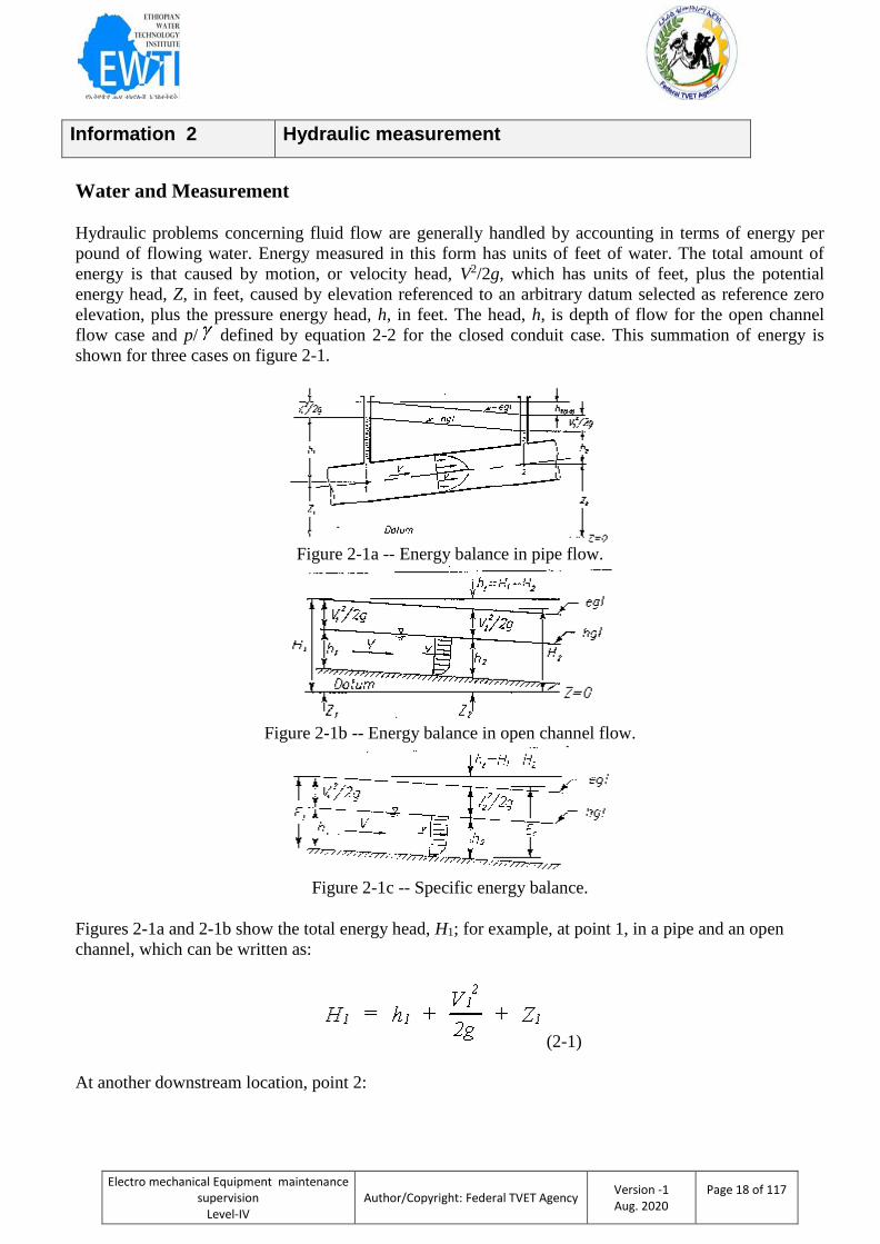
shown for three cases on figure 2-1.
Figure 2-1a -- Energy balance in pipe flow.
Figure 2-1b -- Energy balance in open channel flow.
Figure 2-1c -- Specific energy balance.
Figures 2-1a and 2-1b show the total energy head, H1; for example, at point 1, in a pipe and an open
channel, which can be written as:
(2-1)
At another downstream location, point 2:
Electro mechanical Equipment maintenance supervision
Level-IV
Author/Copyright: Federal TVET Agency Version -1 Aug. 2020
Page 19 of 117
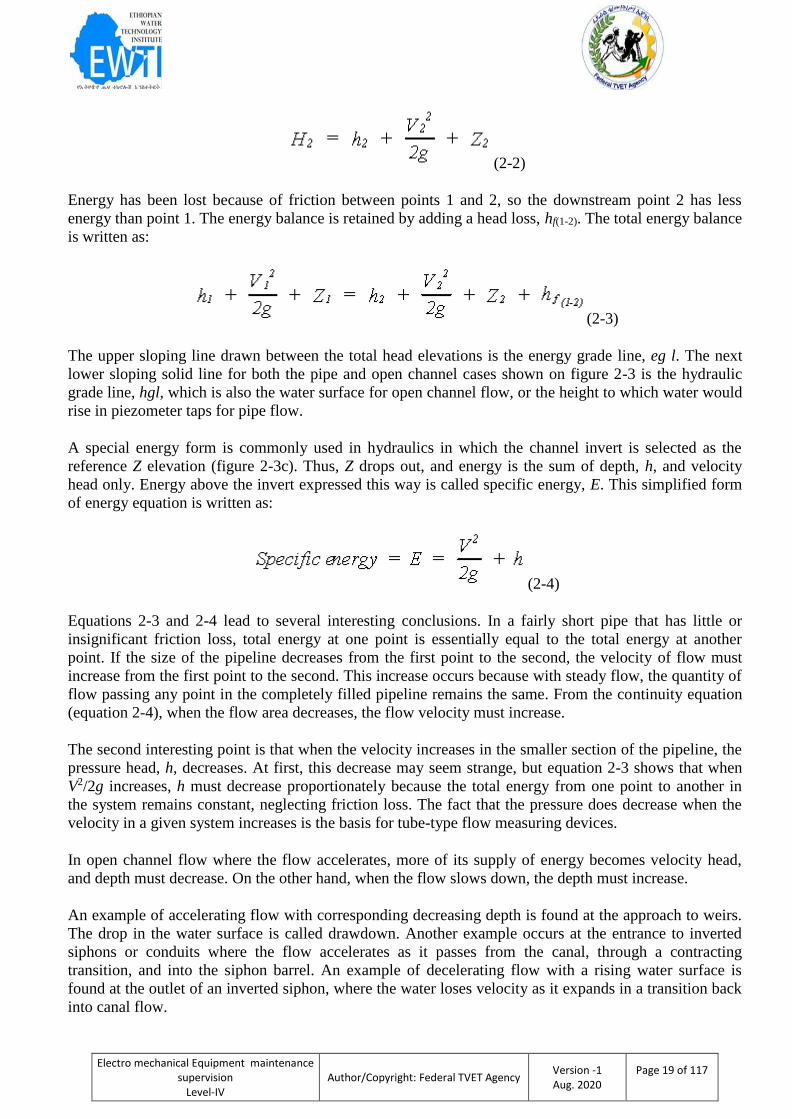
(2-2)
Energy has been lost because of friction between points 1 and 2, so the downstream point 2 has less
energy than point 1. The energy balance is retained by adding a head loss, hf(1-2). The total energy balance
is written as:
(2-3)
The upper sloping line drawn between the total head elevations is the energy grade line, eg l. The next
lower sloping solid line for both the pipe and open channel cases shown on figure 2-3 is the hydraulic
grade line, hgl, which is also the water surface for open channel flow, or the height to which water would
rise in piezometer taps for pipe flow.
A special energy form is commonly used in hydraulics in which the channel invert is selected as the
reference Z elevation (figure 2-3c). Thus, Z drops out, and energy is the sum of depth, h, and velocity
head only. Energy above the invert expressed this way is called specific energy, E. This simplified form
of energy equation is written as:
(2-4)
Equations 2-3 and 2-4 lead to several interesting conclusions. In a fairly short pipe that has little or
insignificant friction loss, total energy at one point is essentially equal to the total energy at another
point. If the size of the pipeline decreases from the first point to the second, the velocity of flow must
increase from the first point to the second. This increase occurs because with steady flow, the quantity of
flow passing any point in the completely filled pipeline remains the same. From the continuity equation
(equation 2-4), when the flow area decreases, the flow velocity must increase.
The second interesting point is that when the velocity increases in the smaller section of the pipeline, the
pressure head, h, decreases. At first, this decrease may seem strange, but equation 2-3 shows that when
V2/2g increases, h must decrease proportionately because the total energy from one point to another in
the system remains constant, neglecting friction loss. The fact that the pressure does decrease when the
velocity in a given system increases is the basis for tube-type flow measuring devices.
In open channel flow where the flow accelerates, more of its supply of energy becomes velocity head,
and depth must decrease. On the other hand, when the flow slows down, the depth must increase.
An example of accelerating flow with corresponding decreasing depth is found at the approach to weirs.
The drop in the water surface is called drawdown. Another example occurs at the entrance to inverted
siphons or conduits where the flow accelerates as it passes from the canal, through a contracting
transition, and into the siphon barrel. An example of decelerating flow with a rising water surface is
found at the outlet of an inverted siphon, where the water loses velocity as it expands in a transition back
into canal flow.

Electro mechanical Equipment maintenance supervision
Level-IV
Author/Copyright: Federal TVET Agency Version -1 Aug. 2020
Page 20 of 117
Flumes are excellent examples of measuring devices that take advantage of the fact that changes in depth
occur with changes in velocity. When water enters a flume, it accelerates in a converging section. The
acceleration of the flow causes the water surface to drop a significant amount. This change in depth is
directly related to the rate of flow

Electro mechanical Equipment maintenance supervision
Level-IV
Author/Copyright: Federal TVET Agency Version -1 Aug. 2020
Page 21 of 117
Self check 2 Written test.
Direction : write the answer for the following questions. Use the Answer sheet provided
1. What are excellent examples of measuring devices that take advantage of the fact that changes in
depth occur with changes in velocity?
2. The drop in the water surface is called _________________.
3. Energy above the invert expressed this way is called _______________ ,it simplified with what?
Answer Sheet-1
Name: _________________Date: ______________
Answer
1. ______________________________________________________________________________
______________________________________________________________________________
_______________________________
2. ______________________________________________________________________________
___________________________________________
3. ______________________________________________________________________________
_________________________________________________
Note: Satisfactory rating - 5 points Unsatisfactory - below 5 points
You can ask you teacher for the copy of the correct answers.
Score = ___________
Rating: ____________
Electro mechanical Equipment maintenance supervision
Level-IV
Author/Copyright: Federal TVET Agency Version -1 Aug. 2020
Page 22 of 117
Information sheet 3 Applying Hydraulic software
Computer Applications
It is very important for students (and practicing engineers) to fully understand the
methodologies behind hydraulic computations. Once these concepts are understood, the
solution process can become repetitive and tedious—the type of procedure that is well-suited to
computer analysis. There are several advantages to using computerized solutions for common
hydraulic problems: The amount of time to perform an analysis can be greatly reduced.
Computer solutions can be more detailed than hand calculations. Performing a solution
manually often requires many simplifying assumptions. The solution process may be less error-
prone. Unit conversion and the rewriting of equations to solve for any variable are just two
examples of mistakes frequently introduced with hand calculations. A well-tested computer
program helps to avoid these algebraic and numeric errors. The solution is easily documented
and reproducible. Because of the speed and accuracy of a computer model, more comparisons
and design trials can be performed. The result is the exploration of more design options, which
eventually leads to better, more efficient designs. In order to prevent an “overload” of data, this
chapter deals primarily with steady-state computations. After all, an introduction to hydraulic
calculations is tricky enough without throwing in the added complexity of a constantly changing
system
The assumption that a system is under steady-state conditions is oftent perfectly acceptable.
Minor changes that occur over time or irregularities in a channel cross-sectionare frequently
negligible, and a more detailed analysis may not be the most efficient or effective use of time
and resources. There are circumstances when an engineer may be called upon to provide a
more detailed analysis, including unsteady flow computations. For a storm sewer, the flows
may rise and fall over time as a storm builds and subsides. For water distribution piping, a
pressure wave may travel through the system when a valve is closed abruptly (the same
“water-hammer” effect can probably be heard in your house if you close a faucet quickly). As an
engineer, it is important to understand the purpose of an analysis; otherwise, appropriate
methods and tools to meet that purpose cannot be selected.
Flow Master
Flow Master is an easy-to-use program that helps civil engineers with the hydraulic design and
analysis of pipes, gutters, inlets, ditches, open channels, weirs, and orifices. Flow Master
computes flows and pressures in conduits and channels using common head loss equations
such as Darcy-We is bach, Manning’s, Kutter’s, and Hazen-Williams. The program’s flexibility
Electro mechanical Equipment maintenance supervision
Level-IV
Author/Copyright: Federal TVET Agency Version -1 Aug. 2020
Page 23 of 117
allows the user to choose an unknown variable and automatically compute the solution after
entering known parameters. Flow Master also calculates rating tables and plots curves and
cross-sections. You can view the output on the screen, copy it to the Windows clipboard, save
it to a file, or print it on any standard printer. Flow Master data can also be viewed and edited
using tabular reports called Flex Tables. Flow Master enables you to create an unlimited
number of worksheets to analyze uniform pressure-pipe or open-channel sections, including
irregular sections (such as natural streams or odd-shaped man-made sections). Flow Master
does not work with networked systems such as a storm sewer network or a pressure pipe
network. For these types of analyses, Storm CAD, Water CAD, or Sewer CAD should be used
instead. The theory and background used by Flow Master have been reviewed in this chapter
and can be accessed via the Flow Master on-line help system. General information about
installing and running Haestad Methods software can be found in Appendix A. Flow Master
replaces solutions such as nomographs, spreadsheets, and BASIC programs. Because Flow
Master gives you immediate results, you can quickly generate output for a large number of
situations. For example, you can use Flow Master to: Analyze various hydraulic designs.
Evaluate different kinds of flow elements Generate professional-looking reports for clients and
review agencies Computer Applications in Hydraulic Engineering
Tutorial Example
The following solution gives step-by-step instructions on how to solve an example problem
using the Flow Master computer program (included on the CD-ROM that accompanies this
textbook) developed by Haestad Methods. Problem Statement Using Manning’s equation,
design a triangular concrete channel with equal side slopes, a longitudinal slope of 5%, a peak
flow capacity of 0.6 m3/s, and a maximum depth of0.3. Also, design a concrete trapezoidal
channel with equal side slopes and a base width of 0.2 that meets the same criteria. Create a
cross-section of each channel and a curve of discharge versus depth for each channel.
Assume the water is at 20°C. Solution Upon opening Flow Master, click Create New Project in
the Welcome to Flow Master dialog. Enter a filename and click Save. ƒƒƒƒƒƒƒƒƒ
Select Triangular Channel from the Create a New Worksheet dialog and click OK. In the
Triangular Channel dialog, select Manning’s Formulafrom the FrictionMethod pull-down menu.
Enter a label for the worksheet and clickOK.Select Global Options from the Options menu and
change the unit system to System International, if it has not already been done, by selecting it
from the pull-down menu in the Unit System field. Click OK to exit the dialog. If you changed
the unit system, you will be prompted to confirm the unit change. Click Yes. The worksheet
dialog should appear. Because discharge, channel slope, and depth aregiven, the variable you
Electro mechanical Equipment maintenance supervision
Level-IV
Author/Copyright: Federal TVET Agency Version -1 Aug. 2020
Page 24 of 117
need to solve for is the side slopes of the channel. Select Equal Side Slopes from the Solve for:
menu at the top of the dialog. Enter the channel slope (you can change the units to percent by
double left-clicking the units), depth, and discharge into the appropriate fields and select the
Manning’s n for concrete. ClickSolve. The equal side slopes should be 1.54 H:V. To design the
trapezoidal section, first click Close on the triangular section worksheet to save it. Then click
Create... at the bottom of the Worksheet List. Select the Trapezoidal Channel and OK. Repeat
the same steps as before to design the triangular channel. The equal side slopes should be
0.80 H:V. Click Close to exit the worksheet.
Creating Channel Cross-Sections
Open the triangular section worksheet by highlighting it and selecting the Open button ƒ
Click the Report button on the bottom of the triangular channel worksheet. Select Cross
Section..
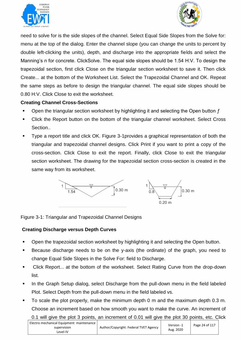
Type a report title and click OK. Figure 3-1provides a graphical representation of both the
triangular and trapezoidal channel designs. Click Print if you want to print a copy of the
cross-section. Click Close to exit the report. Finally, click Close to exit the triangular
section worksheet. The drawing for the trapezoidal section cross-section is created in the
same way from its worksheet.
Figure 3-1: Triangular and Trapezoidal Channel Designs
Creating Discharge versus Depth Curves
Open the trapezoidal section worksheet by highlighting it and selecting the Open button.
Because discharge needs to be on the y-axis (the ordinate) of the graph, you need to
change Equal Side Slopes in the Solve For: field to Discharge.
Click Report... at the bottom of the worksheet. Select Rating Curve from the drop-down
list.
In the Graph Setup dialog, select Discharge from the pull-down menu in the field labeled
Plot. Select Depth from the pull-down menu in the field labeled vs.
To scale the plot properly, make the minimum depth 0 m and the maximum depth 0.3 m.
Choose an increment based on how smooth you want to make the curve. An increment of
0.1 will give the plot 3 points, an increment of 0.01 will give the plot 30 points, etc. Click
Electro mechanical Equipment maintenance supervision
Level-IV
Author/Copyright: Federal TVET Agency Version -1 Aug. 2020
Page 25 of 117
OK. Click Print Preview at the top of the window, and then click Print to print out a report
featuring the rating curve you have just created. Click Close to exit the Print Preview
window. Click Close again to exit the Plot Window.
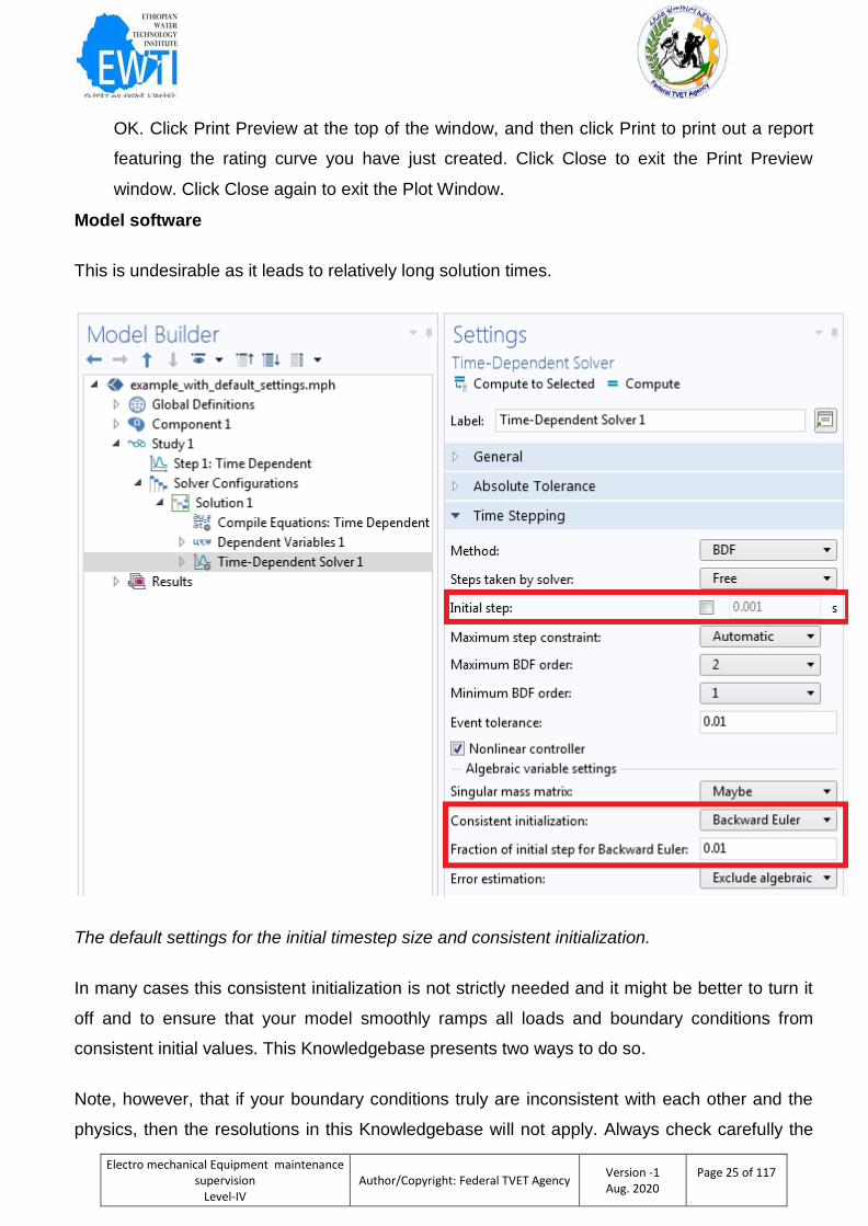
Model software
This is undesirable as it leads to relatively long solution times.
The default settings for the initial timestep size and consistent initialization.
In many cases this consistent initialization is not strictly needed and it might be better to turn it
off and to ensure that your model smoothly ramps all loads and boundary conditions from
consistent initial values. This Knowledgebase presents two ways to do so.
Note, however, that if your boundary conditions truly are inconsistent with each other and the
physics, then the resolutions in this Knowledgebase will not apply. Always check carefully the
Electro mechanical Equipment maintenance supervision
Level-IV
Author/Copyright: Federal TVET Agency Version -1 Aug. 2020
Page 26 of 117
applied loads and boundary conditions for consistency. The recommendations in this
Knowledgebase apply to well-posed problems.
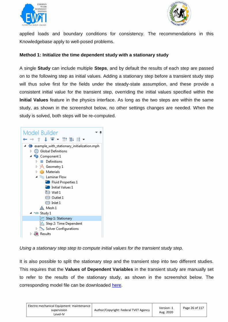
Method 1: Initialize the time dependent study with a stationary study
A single Study can include multiple Steps, and by default the results of each step are passed
on to the following step as initial values. Adding a stationary step before a transient study step
will thus solve first for the fields under the steady-state assumption, and these provide a
consistent initial value for the transient step, overriding the initial values specified within the
Initial Values feature in the physics interface. As long as the two steps are within the same
study, as shown in the screenshot below, no other settings changes are needed. When the
study is solved, both steps will be re-computed.
Using a stationary step step to compute initial values for the transient study step.
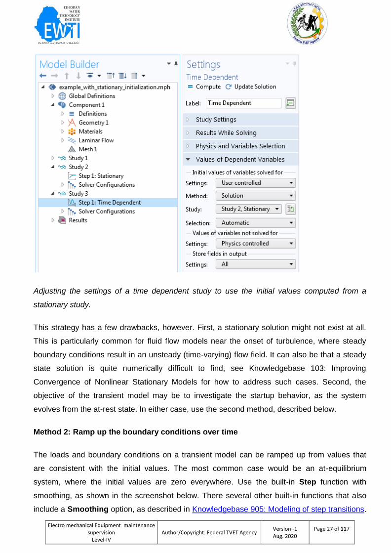
It is also possible to split the stationary step and the transient step into two different studies.
This requires that the Values of Dependent Variables in the transient study are manually set
to refer to the results of the stationary study, as shown in the screenshot below. The
corresponding model file can be downloaded here.
Electro mechanical Equipment maintenance supervision
Level-IV
Author/Copyright: Federal TVET Agency Version -1 Aug. 2020
Page 27 of 117
Adjusting the settings of a time dependent study to use the initial values computed from a
stationary study.
This strategy has a few drawbacks, however. First, a stationary solution might not exist at all.
This is particularly common for fluid flow models near the onset of turbulence, where steady
boundary conditions result in an unsteady (time-varying) flow field. It can also be that a steady
state solution is quite numerically difficult to find, see Knowledgebase 103: Improving
Convergence of Nonlinear Stationary Models for how to address such cases. Second, the
objective of the transient model may be to investigate the startup behavior, as the system
evolves from the at-rest state. In either case, use the second method, described below.
Method 2: Ramp up the boundary conditions over time
The loads and boundary conditions on a transient model can be ramped up from values that
are consistent with the initial values. The most common case would be an at-equilibrium
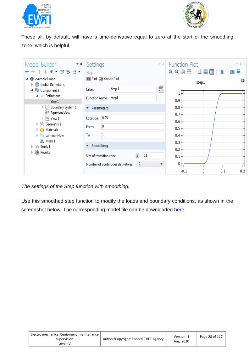
system, where the initial values are zero everywhere. Use the built-in Step function with
smoothing, as shown in the screenshot below. There several other built-in functions that also
include a Smoothing option, as described in Knowledgebase 905: Modeling of step transitions.
Electro mechanical Equipment maintenance supervision
Level-IV
Author/Copyright: Federal TVET Agency Version -1 Aug. 2020
Page 28 of 117
These all, by default, will have a time-derivative equal to zero at the start of the smoothing
zone, which is helpful.
The settings of the Step function with smoothing.
Use this smoothed step function to modify the loads and boundary conditions, as shown in the
screenshot below. The corresponding model file can be downloaded here.
Electro mechanical Equipment maintenance supervision
Level-IV
Author/Copyright: Federal TVET Agency Version -1 Aug. 2020
Page 29 of 117
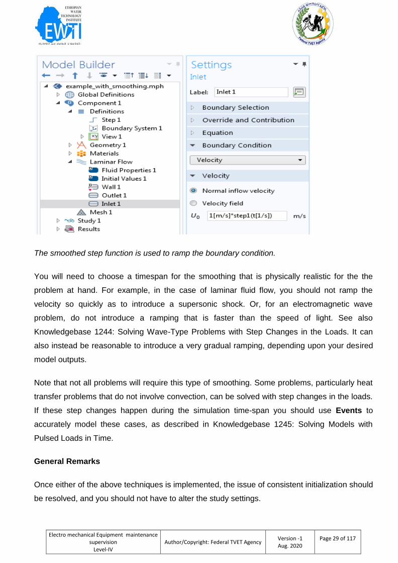
The smoothed step function is used to ramp the boundary condition.
You will need to choose a timespan for the smoothing that is physically realistic for the the
problem at hand. For example, in the case of laminar fluid flow, you should not ramp the
velocity so quickly as to introduce a supersonic shock. Or, for an electromagnetic wave
problem, do not introduce a ramping that is faster than the speed of light. See also
Knowledgebase 1244: Solving Wave-Type Problems with Step Changes in the Loads. It can
also instead be reasonable to introduce a very gradual ramping, depending upon your desired
model outputs.
Note that not all problems will require this type of smoothing. Some problems, particularly heat
transfer problems that do not involve convection, can be solved with step changes in the loads.
If these step changes happen during the simulation time-span you should use Events to
accurately model these cases, as described in Knowledgebase 1245: Solving Models with
Pulsed Loads in Time.
General Remarks
Once either of the above techniques is implemented, the issue of consistent initialization should
be resolved, and you should not have to alter the study settings.

Electro mechanical Equipment maintenance supervision
Level-IV
Author/Copyright: Federal TVET Agency Version -1 Aug. 2020
Page 30 of 117
If you do continue to have issues with convergence, it can be that your model is not meshed
finely enough, in which case you should perform a mesh refinement study as described in
Knowledgebase 1261: Performing a Mesh Refinement Study. It can also be that your model is
highly nonlinear, in which case see Knowledgebase 1127: Improving convergence in nonlinear
time dependent models.
Electro mechanical Equipment maintenance supervision
Level-IV
Author/Copyright: Federal TVET Agency Version -1 Aug. 2020
Page 31 of 117
Self-Check -3 Written Test
Direction I: Choose the best answer for the following questions. Use the Answer sheet
provided in the next page:Each question worth one point
1. Which step is considered developing sampling plan?
A/ Selecting sampling size B/Identifying of parameters
C/ Design of sampling scheme D/ All
2. Which one of these is not a disadvantage of composite samples?
A/ Loss of analyze relationships in individual samples
B/ Reduced costs of analyzing of samples
C/potential dilution of analyzes below detection levels
D/ Increase the possibility of analyze interaction.
3-------------- is atype of sample usually taken when you want information specific to a particular
sampling location, time or distinct areas within a sampling location:
A/ Composite sample B/ Grab sample C/ Analyze D/ All
4. Types of samples usually taken when we want an average representation of a sampling
location or time are-------. A/Grab sample B/ Composite sample C/Discreet grab
sample D/ None
5. A properly taken grab sample is a snap shot of the quality of the water at the exact time and
place the sample was taken.
A/ True B/ False
Answer Sheet-1
Name: _________________________ Date: _______________
Choice Questions
1________ 4.__________
2._______ 5.__________
3_______
Score = ___________
Rating: ____________
Note: Satisfactory rating - 5 points Unsatisfactory - below 5points
You can ask you teacher for the copy of the correct answers.
Electro mechanical Equipment maintenance supervision
Level-IV
Author/Copyright: Federal TVET Agency Version -1 Aug. 2020
Page 32 of 117
Information 4 Identifying standard process inconsistent data on
flow conditions.
Introduction
A common mistake when setting up transient models is to have initial conditions that are
inconsistent with the loads and boundary conditions. This occurs most often when running
transient fluid flow studies, but the same type of issue can occur in any time-dependent model.
You may observe the solver taking very small time steps at the beginning of the simulation, or
the solver will report an error message similar to:
Failed to find consistent initial values.
Last time step is not converged.
Solution
Background
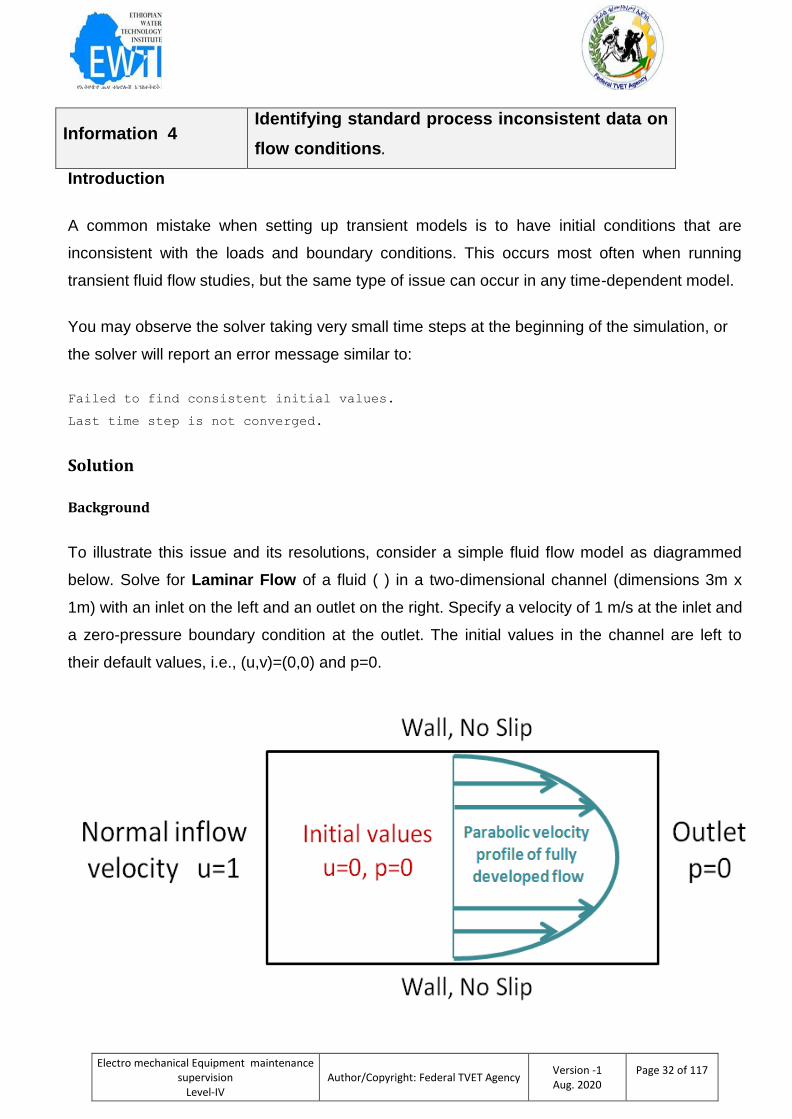
To illustrate this issue and its resolutions, consider a simple fluid flow model as diagrammed
below. Solve for Laminar Flow of a fluid ( ) in a two-dimensional channel (dimensions 3m x
1m) with an inlet on the left and an outlet on the right. Specify a velocity of 1 m/s at the inlet and
a zero-pressure boundary condition at the outlet. The initial values in the channel are left to
their default values, i.e., (u,v)=(0,0) and p=0.
Electro mechanical Equipment maintenance supervision
Level-IV
Author/Copyright: Federal TVET Agency Version -1 Aug. 2020
Page 33 of 117
Figure 4.1 parabolic velocity profile of fully developed flow
These boundary conditions lead to a mismatch between the value of the velocity at the inlet
u=1m/s and the value of the velocity inside the channel u=0 m/s at the beginning of the
simulation, at the initial values from which the transient solver starts to compute the solution.
This is referred to as Inconsistent Initial Values.
COMSOL will, by default, attempt to reconcile inconsistent initial values by taking a small time
step that is a fraction of the initial time step using a Backward Euler method. By default, the
initial time step is automatically determined based upon the total simulation time span, but it is
possible to manually set the initial time step and also to change the fraction of that initial step
used by the Backward Euler method for the consistent initialization. These settings will affect
the results of the consistent initialization procedure. The consistent initialization may fail if the
Backward Euler step is too large or the boundary conditions truly are inconsistent. More
commonly the results may be very far from what is expected, and the solver will likely need to
take very small time steps at the beginning of the simulation to evolve from this solution. This is
undesirable as it leads to relatively long solution times.

Electro mechanical Equipment maintenance supervision
Level-IV
Author/Copyright: Federal TVET Agency Version -1 Aug. 2020
Page 34 of 117
Self check 4 Written test.
Direction: write the answer for the following questions. Use the Answer sheet provided
1. What is the common problem or mistake in flow condition?
2. COMSOL will, by default, attempt to reconcile inconsistent initial values by taking a small
time step that is a fraction of the initial time step using a _______________________.
3. What settings will affect the results of the consistent initialization procedure and in what
case it fail?
Answer sheet
Name: _________________Date: ______________
Answer
1. ______________________________________________________________________________
______________________________________________________________________________
_______________________________
2. ______________________________________________________________________________
___________________________________________
3. ______________________________________________________________________________
_________________________________________________
Note: Satisfactory rating - 5 points Unsatisfactory - below 5 points
You can ask you teacher for the copy of the correct answers.
Electro mechanical Equipment maintenance supervision
Level-IV
Author/Copyright: Federal TVET Agency Version -1 Aug. 2020
Page 35 of 117
Instruction Sheet-2 Learning guide 43: Calculate hydraulic and energy gradient
for pipeline
This learning guide is developed to provide you the necessary information regarding the
following content coverage and topics:
Standard formulae
Pipeline design charts
Roughness coefficients
Calculating pipe line system using hydraulic gradient line
Calculating pipe discharges
This guide will also assist you to attain the learning outcome stated in the cover page.
Specifically, upon completion of this Learning Guide, you will be able to:
.Measurements are reviewed and compared against expected trends.
Standard processes and software are used to check, edit, verify and audit data.
Standard processes are used to identify, estimate, adjust and justify data and review inconsistent data on flow conditions.
Records are prepared in a format suitable for dissemination
Learning Instructions:
1. Read the specific objectives of this Learning Guide.
2. Follow the instructions described below
3. Read the information written in the “Information Sheets 1- 5”. Try to understand what are
being discussed.
4. Accomplish the “Self-checks1,2,3,4and 5 ” in each information sheets on pages 39, 44, 49,
54 and 60
5. Ask from your teacher the key to correction (key answers) or you can request your teacher
to correct your work. (You are to get the key answer only after you finished answering the
Self-checks).
6. After You accomplish self check, ensure you have a formative assessment and get a
satisfactory result; then proceed to the next LG.
Electro mechanical Equipment maintenance supervision
Level-IV
Author/Copyright: Federal TVET Agency Version -1 Aug. 2020
Page 36 of 117
Information Sheet- Standard formula
Calculating Major Losses Using Different Formulas
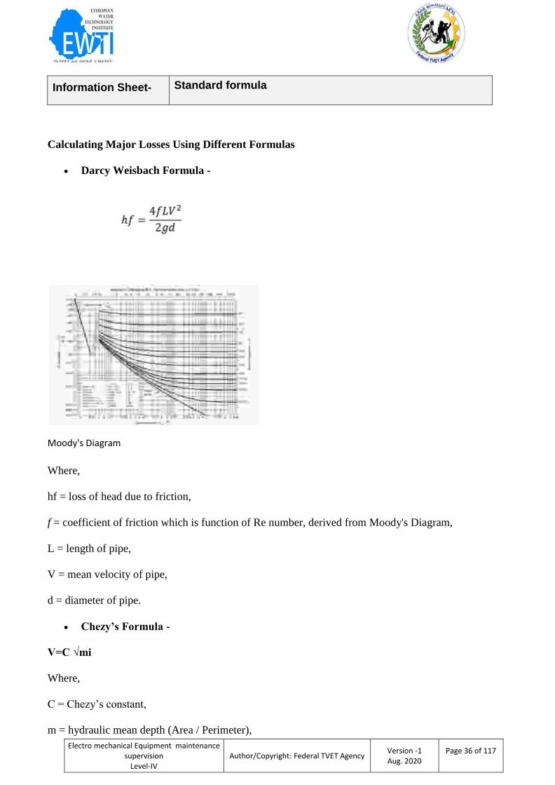
Darcy Weisbach Formula -
Moody's Diagram
Where,
hf = loss of head due to friction,
f = coefficient of friction which is function of Re number, derived from Moody's Diagram,
L = length of pipe,
V = mean velocity of pipe,
d = diameter of pipe.
Chezy’s Formula -
V=C √mi
Where,
C = Chezy’s constant,
m = hydraulic mean depth (Area / Perimeter),
Electro mechanical Equipment maintenance supervision
Level-IV
Author/Copyright: Federal TVET Agency Version -1 Aug. 2020
Page 37 of 117
i = hf / L, which is head loss of head per unit length of pipe.
Hazen-Williams Formula -
Where,
h = head loss (m)
D = diameter (m)
V = velocity (m/s)
C = Hazen-Williams C-factor
L = length (m)
k = 6.79 for V in m/s, D in m or
The C-factor ranges between 0 to 150 depending on the material and age of the pipe.
Modified Hazen-Williams Formula -
where,
V = velocity of flow in m/s,
Cr = pipe roughness coefficient, ( 1 for smooth pipes; < 1 for rough pipes),
r = hydraulic radius in m,
S = friction slope,
h = friction head loss in m.
Difference between the Darcy Weisbach and Hazen-Williams formulas:

Electro mechanical Equipment maintenance supervision
Level-IV
Author/Copyright: Federal TVET Agency Version -1 Aug. 2020
Page 38 of 117
As a part of academic curriculum, Darcy Weisbach formula has enjoyed much popularity as compared to
any other formula owning to extreme precision in the values of the resulting head loss.
But, in practice, the engineers are challenged with high time consumption in determining the value of f -
coefficient of friction for every pipe using Moody's Diagram. Because of this reason, its popularity
among practitioners is very less.
Hazen-Williams formula, perhaps, generates reliable and reasonably precise values of head loss. The
Hazen Williams C-factor ranges between 0 to 150. Rougher the pipe is, smaller would be the value of C
and smoother the pipe is, higher would be the value of C.
Self-Check - 1 Written Test

Electro mechanical Equipment maintenance supervision
Level-IV
Author/Copyright: Federal TVET Agency Version -1 Aug. 2020
Page 39 of 117
Directions: Answer all the questions listed below. Use the Answer sheet provided in the next
page:
1. Try to draw moody diagram.
2. Write the Modified Hazen-Williams Formula. 3. What is Difference between the Darcy Weisbach and Hazen-Williams formulas.
Answer sheet
Answers
7. ________________________________________________________________________
________________________________________________________________________
_________________________________________________
8. ________________________________________________________________________
________________________________________________________________________
______________________________________
9. ________________________________________________________________________
________________________________________________________________________
_______________________________________
Information Sheet- 2 Pipeline design charts
Note: Satisfactory rating - 5 points Unsatisfactory - below 5points
You can ask you teacher for the copy of the correct answers.
Electro mechanical Equipment maintenance supervision
Level-IV
Author/Copyright: Federal TVET Agency Version -1 Aug. 2020
Page 40 of 117
INTRODUCTION TO PIPING SYSTEM
What is piping systems? the piping system install to convey the fluids required for
chemical processes or otherwise between the various equipment and end users and consist of
various components such as valves, fittings, online measuring instruments, etc. is called
as a ‘Piping Systems’
PIPING COMPONENTS
Mechanical element suitable for joining or assembly in to pressure-tight fluid containing piping
systems. Components include pipe, fittings, flanges, gaskets, bolting, valves and
devices such as expansion joint, flexible joints, pressure hoses, traps, strainers, in line portions
of instruments, and separator
Pipe
A pipe or tube is hollow, longitudinal product. ’ A tube’ is a general term used for hollow
product having circular, elliptical or square cross section or for that matter cross section
of any perimeter. A pipe is tubular product of circular cross-section that has specific sizes and
thickness governed by particular dimensional standard
Classifications
Pipe can be classified based on method of manufacture or based on their applications
Method of Manufacture
Seamless pipes are manufactured by drawing or extrusion process
ERW pipes (Electric resistance welded pipes) are formed from a strip which is longitudinally
welded along its length. Welding may be by electric resistance, high frequency, or induction
welding. ERW pipes can also be drawn for obtaining required dimensions and tolerances.
Electro mechanical Equipment maintenance supervision
Level-IV
Author/Copyright: Federal TVET Agency Version -1 Aug. 2020
Page 41 of 117
Pipes in small quantities are manufactured by EFW (Electric fusion welding) Process where in
instead of electric resistance welding, the longitudinal seam is welded by manual or automatic
electric arc process.
There are spiral seam welded pipes, which are large dia pipes 500 NB and above. And pipes
are made by welding a spiral seam produced by forming continues steel skelp in to circular
shape
Centrifugally cast pipes are made by spraying molten metal along a rotating die where the pipes
are cast in shape due to centrifugal action
Classification based on Applications
Pipes are classified as:
- Pressure Pipes or Process pipes
- Line Pipes
- Structural Pipes
Pressure pipes are those which are subjected to fluid pressure and or temperatures. Fluid
pressure in generally internal pressure due to fluid being conveyed or may be external
pressure (i.e. jacketed piping) and are mainly used as plant piping.
Line pipes are mainly used for conveying of the fluid and are subjected to fluid pressure.
These are generally not subjected to high temperatures.
Structural pipes are not used for conveying fluids and therefore not subjected to fluid
pressures or temperatures. They are used as structural components (e.g. handrails,
columns, sleeves etc) and are subjected to static load only.
Pipes Dimensional Standards (ASME B 36.10, ASME B 36.19)
Electro mechanical Equipment maintenance supervision
Level-IV
Author/Copyright: Federal TVET Agency Version -1 Aug. 2020
Page 42 of 117
Diameters: Pipes are designated by Nominal size, starting from 1/8” Nominal size, and
increasing in step
1 Pipes sizes increases in steps of 1/8” to ½” =1/8”,1/4”,3/8”,1/2”, Nominal size
2 Sizes in step of ¼” = ½”,3/4”,1”,1 ¼”,1 ½”
3 In step of ½” up to 4” = 1 ½”, 2”, 2 ½”, 3”, 3 ½”,4”.
4 In step of 1” up to 6” = 4”,5”,6”.
5 In step of 2” up to 36” = 6”,8”,10” ………Etc
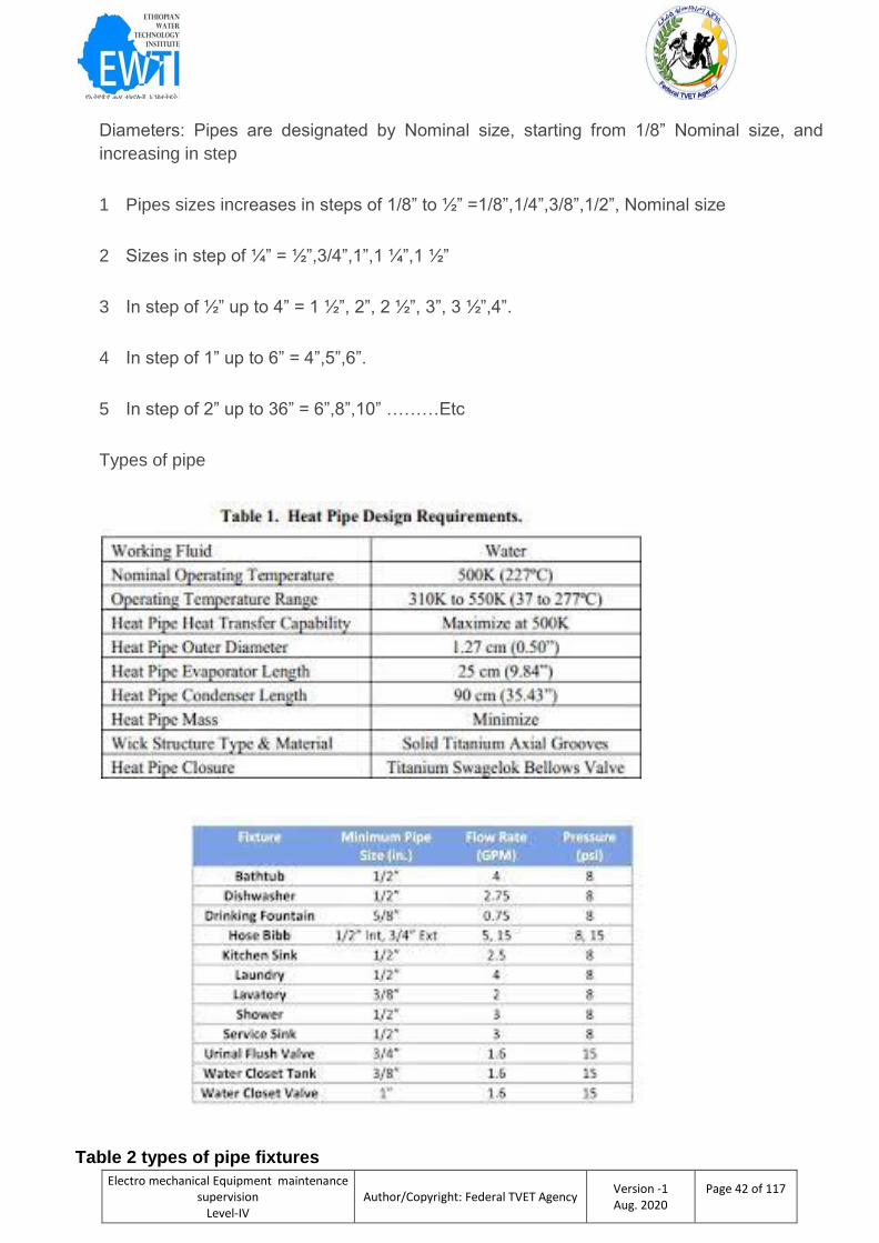
Types of pipe
Table 2 types of pipe fixtures
Electro mechanical Equipment maintenance supervision
Level-IV
Author/Copyright: Federal TVET Agency Version -1 Aug. 2020
Page 43 of 117
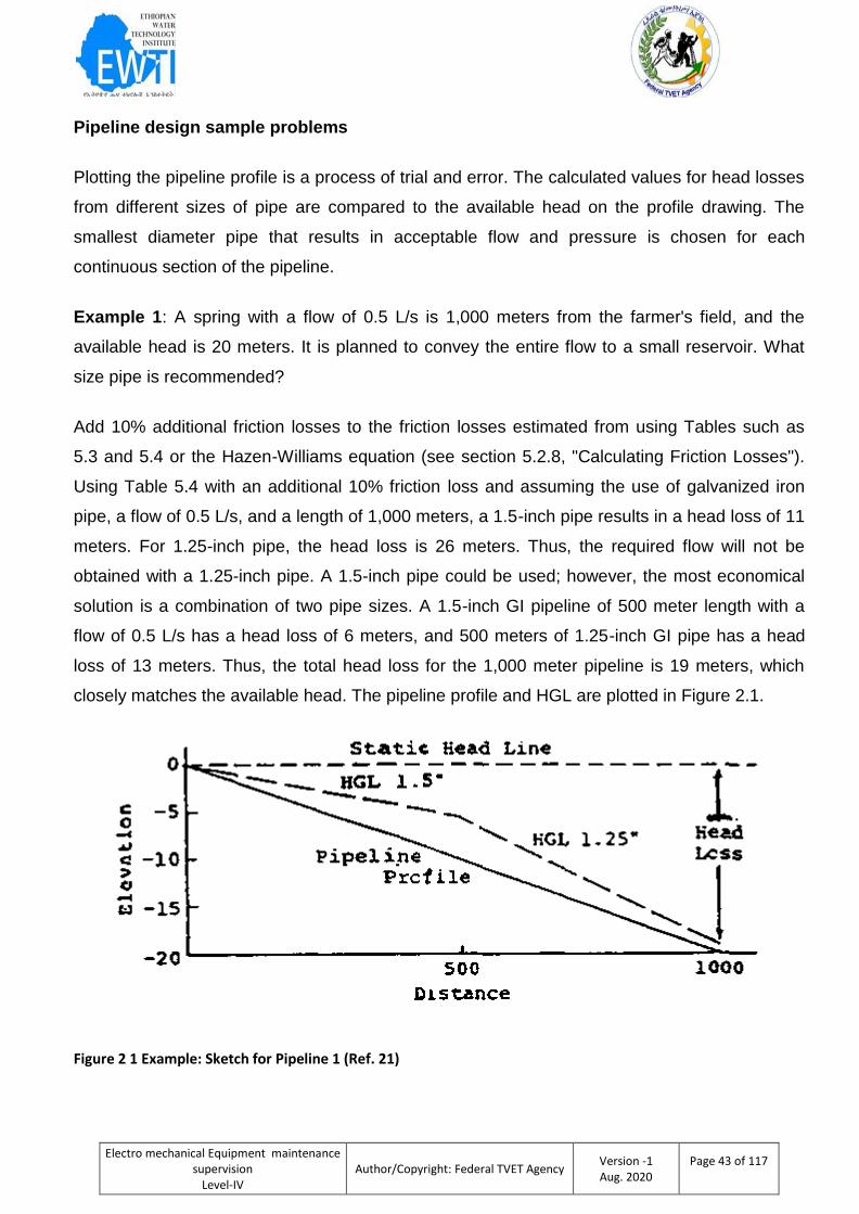
Pipeline design sample problems
Plotting the pipeline profile is a process of trial and error. The calculated values for head losses
from different sizes of pipe are compared to the available head on the profile drawing. The
smallest diameter pipe that results in acceptable flow and pressure is chosen for each
continuous section of the pipeline.
Example 1: A spring with a flow of 0.5 L/s is 1,000 meters from the farmer's field, and the
available head is 20 meters. It is planned to convey the entire flow to a small reservoir. What
size pipe is recommended?
Add 10% additional friction losses to the friction losses estimated from using Tables such as
5.3 and 5.4 or the Hazen-Williams equation (see section 5.2.8, "Calculating Friction Losses").
Using Table 5.4 with an additional 10% friction loss and assuming the use of galvanized iron
pipe, a flow of 0.5 L/s, and a length of 1,000 meters, a 1.5-inch pipe results in a head loss of 11
meters. For 1.25-inch pipe, the head loss is 26 meters. Thus, the required flow will not be
obtained with a 1.25-inch pipe. A 1.5-inch pipe could be used; however, the most economical
solution is a combination of two pipe sizes. A 1.5-inch GI pipeline of 500 meter length with a
flow of 0.5 L/s has a head loss of 6 meters, and 500 meters of 1.25-inch GI pipe has a head
loss of 13 meters. Thus, the total head loss for the 1,000 meter pipeline is 19 meters, which
closely matches the available head. The pipeline profile and HGL are plotted in Figure 2.1.
Figure 2 1 Example: Sketch for Pipeline 1 (Ref. 21)

Electro mechanical Equipment maintenance supervision
Level-IV
Author/Copyright: Federal TVET Agency Version -1 Aug. 2020
Page 44 of 117
Self-Check -2 Written Test
Directions: Answer all the questions listed below. Use the Answer sheet provided in the next
page:
1;-Explain about pipe flow?
2;-What is the standard pipe flow?
3;-write Types of pipes?
4;-write the fixture of pipe design factor?
Answer sheet
Answers
1. _________________________________________________________________________
_________________________________________________________________________
_______________________________________________
2. _________________________________________________________________________
_________________________________________________________________________
____________________________________
3. _________________________________________________________________________
_________________________________________________________________________
_____________________________________
4. _________________________________________________________________________
_________________________________________________________________________
____________________________________________
Note: Satisfactory rating - 5 points Unsatisfactory - below 5points
You can ask you teacher for the copy of the correct answers.
Electro mechanical Equipment maintenance supervision
Level-IV
Author/Copyright: Federal TVET Agency Version -1 Aug. 2020
Page 45 of 117
Information Sheet- 3 Roughness coefficient
Introduction
The resistance to flow in open channels depends on many flow and channel parameters. Out of
the many factors, vegetation is the most important parameter in vegetative channels.
Vegetation in an open channel retards the water flow by causing energy loss through
turbulence and by exerting additional drag forces on the moving liquid. Presence of vegetation
in a channel modify the velocity profiles, and hence the resistance in terms of roughness
coefficients. The roughness coefficients of such channels change with the flow depths and from
sections to sections. Because of this complex nature, it is hard to develop a flow model based
on theoretical calculations and derivations. A laboratory study to explore the effect of vegetation
in terms of rigid cylindrical roughness on the behaviors of Manning's roughness coefficient n,
Chezy's coefficient C and Darcy-Weisbach's friction factor f in an open channel is presented.
The study consists of flume experiments for flows with unsubmerged rigid cylindrical stems of a
concentration and diameter arranged in a regular staggered configuration. The usual practice in
1D analysis is to select a value of n depending on the channel surface roughness and take it as
uniform for the entire surface for all depths of flow. The influences of all the parameters are
assumed to be lumped into a single value of n, C and f. Researches have shown that the
coefficients not only denote the roughness characteristics of a channel but also the energy loss
in the flow. The larger the value of n, the higher is the loss of energy within the flow Different
roughness coefficients are found to vary differently with the non-dimensional hydraulic,
geometric and surface parameters. Behaviours of different resistance coefficients due to
vegetation are discussed and results are summarized and presented. Graphs of aspect ratio
vs. n, C and f respectively are presented
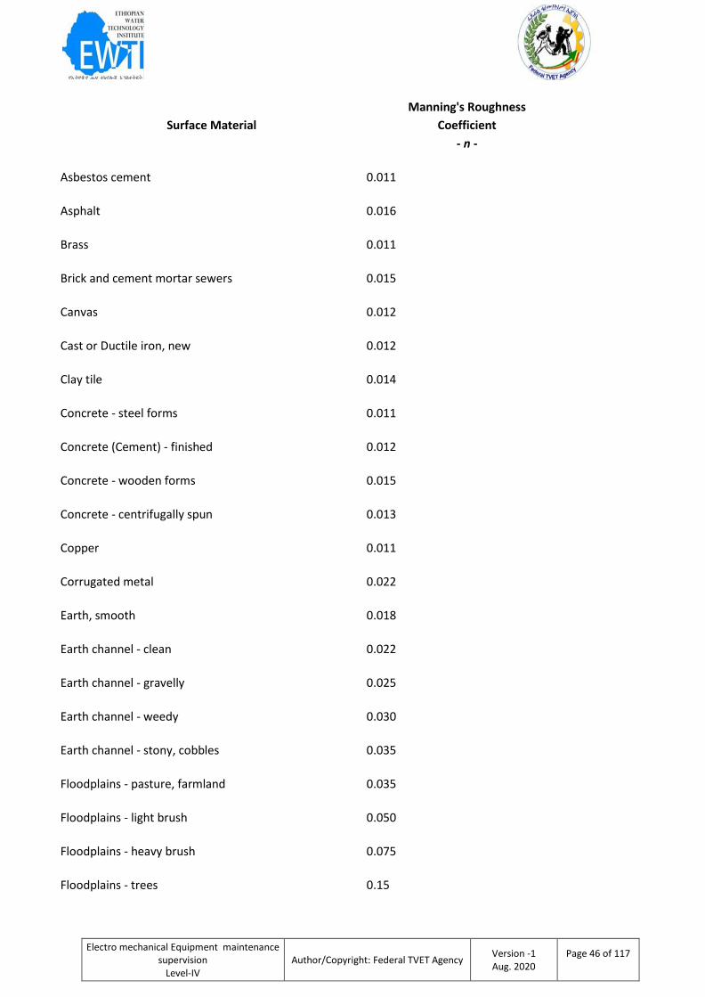
Manning's roughness coefficient
The Manning's roughness coefficient is used in the Manning's formula to calculate flow in open channels.
Coefficients for some commonly used surface materials:
Electro mechanical Equipment maintenance supervision
Level-IV
Author/Copyright: Federal TVET Agency Version -1 Aug. 2020
Page 46 of 117
Surface Material
Manning's Roughness
Coefficient
- n -
Asbestos cement 0.011
Asphalt 0.016
Brass 0.011
Brick and cement mortar sewers 0.015
Canvas 0.012
Cast or Ductile iron, new 0.012
Clay tile 0.014
Concrete - steel forms 0.011
Concrete (Cement) - finished 0.012
Concrete - wooden forms 0.015
Concrete - centrifugally spun 0.013
Copper 0.011
Corrugated metal 0.022
Earth, smooth 0.018
Earth channel - clean 0.022
Earth channel - gravelly 0.025
Earth channel - weedy 0.030
Earth channel - stony, cobbles 0.035
Floodplains - pasture, farmland 0.035
Floodplains - light brush 0.050
Floodplains - heavy brush 0.075
Floodplains - trees 0.15
Electro mechanical Equipment maintenance supervision
Level-IV
Author/Copyright: Federal TVET Agency Version -1 Aug. 2020
Page 47 of 117
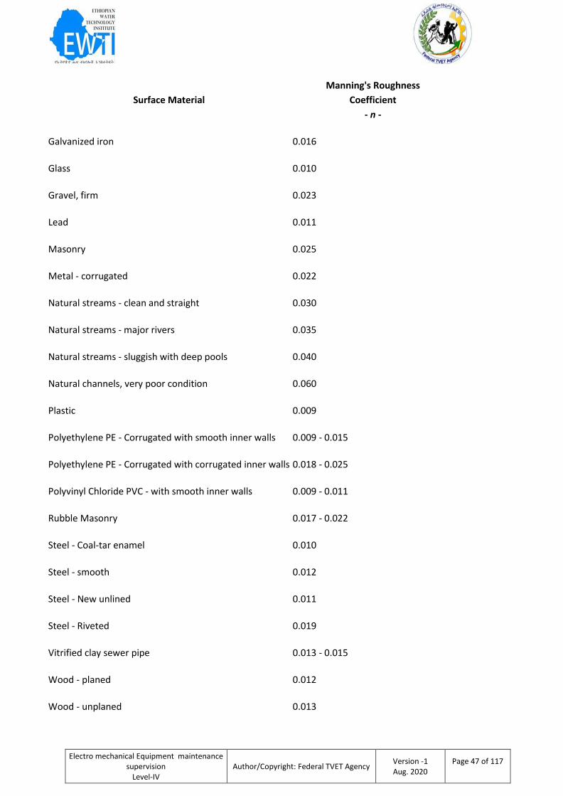
Surface Material
Manning's Roughness
Coefficient
- n -
Galvanized iron 0.016
Glass 0.010
Gravel, firm 0.023
Lead 0.011
Masonry 0.025
Metal - corrugated 0.022
Natural streams - clean and straight 0.030
Natural streams - major rivers 0.035
Natural streams - sluggish with deep pools 0.040
Natural channels, very poor condition 0.060
Plastic 0.009
Polyethylene PE - Corrugated with smooth inner walls 0.009 - 0.015
Polyethylene PE - Corrugated with corrugated inner walls 0.018 - 0.025
Polyvinyl Chloride PVC - with smooth inner walls 0.009 - 0.011
Rubble Masonry 0.017 - 0.022
Steel - Coal-tar enamel 0.010
Steel - smooth 0.012
Steel - New unlined 0.011
Steel - Riveted 0.019
Vitrified clay sewer pipe 0.013 - 0.015
Wood - planed 0.012
Wood - unplaned 0.013

Electro mechanical Equipment maintenance supervision
Level-IV
Author/Copyright: Federal TVET Agency Version -1 Aug. 2020
Page 48 of 117
Surface Material
Manning's Roughness
Coefficient
- n -
Wood stave pipe, small diameter 0.011 - 0.012
Wood stave pipe, large diameter 0.012 - 0.013

Electro mechanical Equipment maintenance supervision
Level-IV
Author/Copyright: Federal TVET Agency Version -1 Aug. 2020
Page 49 of 117
Self-Check -3 Written Test
Directions: Answer all the questions listed below. Use the Answer sheet provided in the next
page:
1. What is roughness coefficient?
2. What are factors that affect roughness coefficient?
Answer Sheet-5
Name: _________________________ Date: _______________
Short answer
1. _____________________________________________________________________
_____________________________________________________________________
_____________________________________________________________________
____________________________
2. _____________________________________________________________________
_____________________________________________________________________
_____________________________________________________________________
_____________________________.
Note: Satisfactory rating – 3 and above points Unsatisfactory - below 3 points
You can ask you teacher for the copy of the correct answers.
Electro mechanical Equipment maintenance supervision
Level-IV
Author/Copyright: Federal TVET Agency Version -1 Aug. 2020
Page 50 of 117
Information Sheet-4 Calculating hydraulic gradient line
Introduction In the flow of a fluid through pipes, it is seen that there is a loss of head. Whilst some of this is due to the effect
of sudden contraction or expansions in the pipe diameter, pipe fittings such as bends and valves and entry and
exit losses, a loss of potential head (i.e. The input of the pipe is higher than the outflow) a significant portion is
due to the friction in the pipe (The Darcy Equation). However in a pipe of uniform cross section, there will be no
loss of velocity head and so the loss of Total Energy will be the result of a loss in Pressure Head.
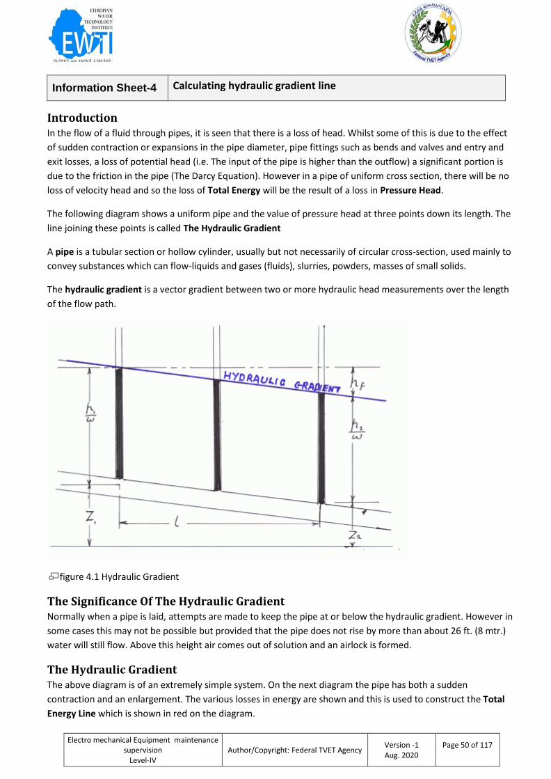
The following diagram shows a uniform pipe and the value of pressure head at three points down its length. The
line joining these points is called The Hydraulic Gradient
A pipe is a tubular section or hollow cylinder, usually but not necessarily of circular cross-section, used mainly to
convey substances which can flow-liquids and gases (fluids), slurries, powders, masses of small solids.
The hydraulic gradient is a vector gradient between two or more hydraulic head measurements over the length
of the flow path.
figure 4.1 Hydraulic Gradient
The Significance Of The Hydraulic Gradient Normally when a pipe is laid, attempts are made to keep the pipe at or below the hydraulic gradient. However in
some cases this may not be possible but provided that the pipe does not rise by more than about 26 ft. (8 mtr.)
water will still flow. Above this height air comes out of solution and an airlock is formed.
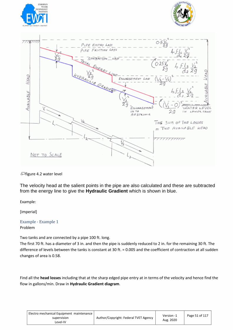
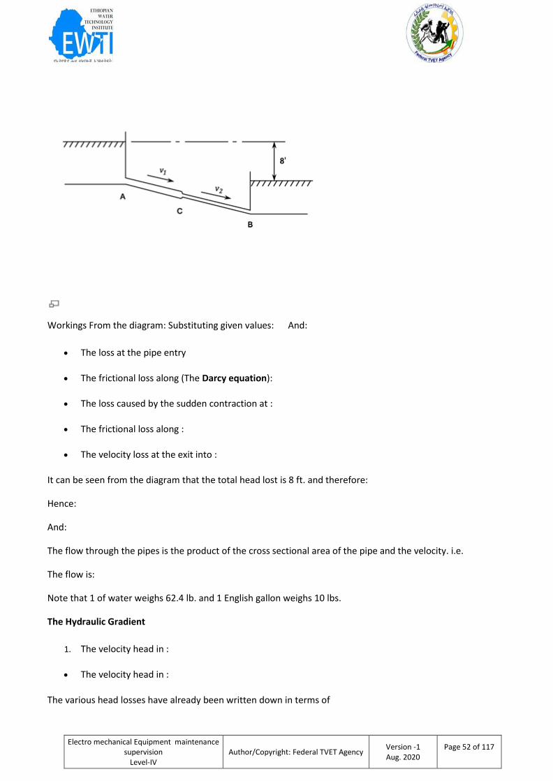
The Hydraulic Gradient The above diagram is of an extremely simple system. On the next diagram the pipe has both a sudden
contraction and an enlargement. The various losses in energy are shown and this is used to construct the Total
Energy Line which is shown in red on the diagram.
Electro mechanical Equipment maintenance supervision
Level-IV
Author/Copyright: Federal TVET Agency Version -1 Aug. 2020
Page 51 of 117
figure 4.2 water level
The velocity head at the salient points in the pipe are also calculated and these are subtracted from the energy line to give the Hydraulic Gradient which is shown in blue.
Example:
[imperial]
Example - Example 1
Problem
Two tanks and are connected by a pipe 100 ft. long.
The first 70 ft. has a diameter of 3 in. and then the pipe is suddenly reduced to 2 in. for the remaining 30 ft. The
difference of levels between the tanks is constant at 30 ft. = 0.005 and the coefficient of contraction at all sudden
changes of area is 0.58.
Find all the head losses including that at the sharp edged pipe entry at in terms of the velocity and hence find the
flow in gallons/min. Draw in Hydraulic Gradient diagram.
Electro mechanical Equipment maintenance supervision
Level-IV
Author/Copyright: Federal TVET Agency Version -1 Aug. 2020
Page 52 of 117
Workings From the diagram: Substituting given values: And:
The loss at the pipe entry
The frictional loss along (The Darcy equation):
The loss caused by the sudden contraction at :
The frictional loss along :
The velocity loss at the exit into :
It can be seen from the diagram that the total head lost is 8 ft. and therefore:
Hence:
And:
The flow through the pipes is the product of the cross sectional area of the pipe and the velocity. i.e.
The flow is:
Note that 1 of water weighs 62.4 lb. and 1 English gallon weighs 10 lbs.
The Hydraulic Gradient
1. The velocity head in :
The velocity head in :
The various head losses have already been written down in terms of
Electro mechanical Equipment maintenance supervision
Level-IV
Author/Copyright: Federal TVET Agency Version -1 Aug. 2020
Page 53 of 117
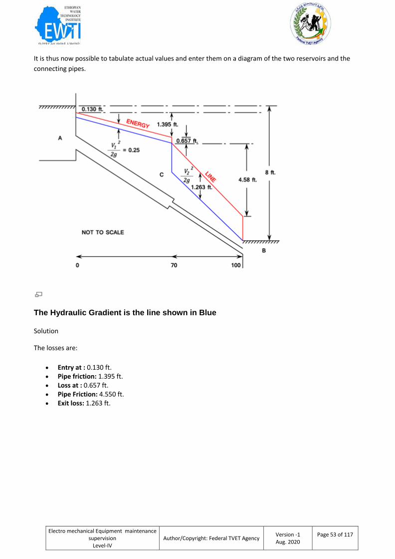
It is thus now possible to tabulate actual values and enter them on a diagram of the two reservoirs and the
connecting pipes.
The Hydraulic Gradient is the line shown in Blue
Solution
The losses are:
Entry at : 0.130 ft. Pipe friction: 1.395 ft. Loss at : 0.657 ft. Pipe Friction: 4.550 ft. Exit loss: 1.263 ft.
Electro mechanical Equipment maintenance supervision
Level-IV
Author/Copyright: Federal TVET Agency Version -1 Aug. 2020
Page 54 of 117
Self-Check -4 Written Test
Direction : calculate the given question and give the answer.
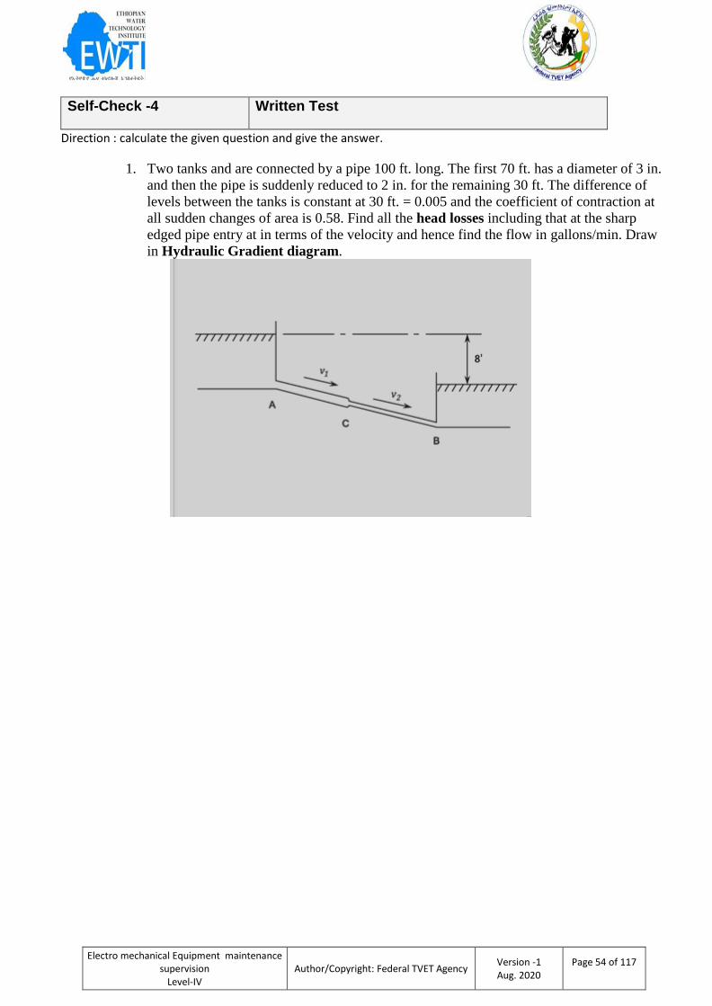
1. Two tanks and are connected by a pipe 100 ft. long. The first 70 ft. has a diameter of 3 in.
and then the pipe is suddenly reduced to 2 in. for the remaining 30 ft. The difference of
levels between the tanks is constant at 30 ft. = 0.005 and the coefficient of contraction at
all sudden changes of area is 0.58. Find all the head losses including that at the sharp
edged pipe entry at in terms of the velocity and hence find the flow in gallons/min. Draw
in Hydraulic Gradient diagram.
Electro mechanical Equipment maintenance supervision
Level-IV
Author/Copyright: Federal TVET Agency Version -1 Aug. 2020
Page 55 of 117
Information sheet 5 Calculating pipe discharges
channel flow: Uniform flow, best hydraulic sections, energy principles, Froude number
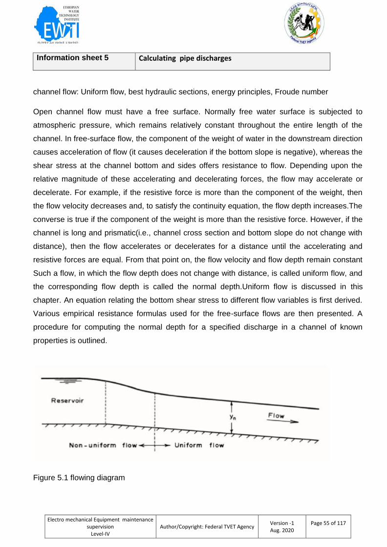
Open channel flow must have a free surface. Normally free water surface is subjected to
atmospheric pressure, which remains relatively constant throughout the entire length of the
channel. In free-surface flow, the component of the weight of water in the downstream direction
causes acceleration of flow (it causes deceleration if the bottom slope is negative), whereas the
shear stress at the channel bottom and sides offers resistance to flow. Depending upon the
relative magnitude of these accelerating and decelerating forces, the flow may accelerate or
decelerate. For example, if the resistive force is more than the component of the weight, then
the flow velocity decreases and, to satisfy the continuity equation, the flow depth increases.The
converse is true if the component of the weight is more than the resistive force. However, if the
channel is long and prismatic(i.e., channel cross section and bottom slope do not change with
distance), then the flow accelerates or decelerates for a distance until the accelerating and
resistive forces are equal. From that point on, the flow velocity and flow depth remain constant
Such a flow, in which the flow depth does not change with distance, is called uniform flow, and
the corresponding flow depth is called the normal depth.Uniform flow is discussed in this
chapter. An equation relating the bottom shear stress to different flow variables is first derived.
Various empirical resistance formulas used for the free-surface flows are then presented. A
procedure for computing the normal depth for a specified discharge in a channel of known
properties is outlined.
Figure 5.1 flowing diagram
Electro mechanical Equipment maintenance supervision
Level-IV
Author/Copyright: Federal TVET Agency Version -1 Aug. 2020
Page 56 of 117
Manning Equation
Since the derivation of the Chezy equation in 1768, several researchers have tried to develop a
rational procedure for estimating the value of Chezy constant, C. However, unlike the Darcy-
Weisbach friction factor for the closed conduits, these attempts have not been very successful,
because C depends upon several parameters in addition to the channel roughness.
French engineer named A. Flamant incorrectly attributed the above equation to an Irishman, R.
Manning, and expressed it in the followingform in 1891
CHEZY’S EQUATION
Pitot Tube
A pitot tube is a pressure measurement instrument used to measurefluidflow velocity. The pitot
tube was invented by theFrenchengineerHenri Pitotin the early 18th centuryand was modified
to its modern form in the mid-19th century by French scientistHenry Darcy.It is widely used to
determine theairspeedof anaircraft, water speed of a boat, and to measure liquid, air and gas
flow velocities in industrial applications.The pitot tube is used to measure the local flow
velocity at a given point in the flow stream and not the average flow velocity in the pipe or
conduit.The basic pitot tube consists of a tube pointing directly into the fluid flow. As this tube
contains fluid, a pressure can be measured; the moving fluid is brought to rest (stagnates) as
there is no outlet to allow flow to continue. This pressure is the stagnation pressureof the fluid,
also known as the total pressure or (particularly in aviation) the pitot pressure.The measured
stagnation pressure cannot itself beused to determine the fluid flow velocity (airspeed in
aviation). However,Bernoulli’sstates:Stagnation pressure = static pressure + dynamic
pressure
CURRENT METER
Electro mechanical Equipment maintenance supervision
Level-IV
Author/Copyright: Federal TVET Agency Version -1 Aug. 2020
Page 57 of 117
Acurrent meterisoceanographicdevice forflow measurementby mechanical (rotor current
meter), tilt (Tilt Current Meter), acoustical (ADCP) or electrical means.
MEASUREMENT PRINCIPLES
a. Mechanical current meters are mostly based on counting the rotations of a propeller and are
thusrotor current meters. A mid-20th-century realization is theEkman current meterwhich drops
balls into a container to count the number of rotations.
b.Acoustic Thereare two basic types of acoustic current meters: Doppler and Travel Time.
Both methods use a ceramic transducer to emit a sound into the water.Doppler instruments are
more common.An instrument of this type is theAcoustic Doppler Current Profiler(ADCP)which
measures thewater currentvelocitiesover a depth range using theDoppler effectofsound
wavesscattered back from particles within the water column. The ADCPs use the traveling time
of the sound to determine the position of the moving particles. Single-point devices use again
the Doppler shift, but ignoring the traveling times. Such a single point Doppler Current Sensor
(DCS) has a typical velocity range of 0 to 300cm/s.Travel time instruments determine water
velocity by at least two acoustic signals, one up stream and one down stream.
c. Electromagnetic Induction This novel approach is for instance employed in the Florida
Strait where electromagnetic induction in submerged telephone cableis used to estimate the
through-flow through the gatewayand the complete setup can be seen asone huge current
meter. it is possible to evaluate the variability of the averaged horizontal flow by measuring the
induced electric currents. The method has a minor vertical weighting effect due to small
conductivity changes at different depths.
d.Tilt. current meters operate under the drag-tilt principle. They consist of a sub-surface buoy
that is anchored to the sea floor with a flexible line or tether. The float tilts as a function of its
shape, buoyancy and the water velocity. Once the characteristics of a given buoy are known,
the velocity can be determined by measuring the angle of the buoy.A Tilt Current Meter is
typically deployed on the bottom with an anchor but may be deployed on lobster traps or other
convenient anchors of opportunity.
VENTURIMETER
Venturimeter is a device used for measuring the rate of flow of a fluid flowing through a pipe. It
consists of three parts:• A short converging part
Electro mechanical Equipment maintenance supervision
Level-IV
Author/Copyright: Federal TVET Agency Version -1 Aug. 2020
Page 58 of 117
Throat Diverging partLet d1 = diameter at the inlet (section 1)p1 = pressure at section 1v1 =
velocity at section 1A1= area at section1 d2, p2, v2, A2 are the corresponding values at the
throat (section 2) Applying Bernoulli’s equations at sections 1 and 2, we get
ORIFICE METER
An orifice meter is a conduit and a restriction to create a pressure drop. An hour glass is a form
of orifice. A nozzle, venturi or thin sharp edged orifice can be used as the flow restriction. In
order to use any of these devices for measurement it is necessary to empirically calibrate them.
That is, pass a known volume through the meter and note the reading in order to provide a
standard for measuring other quantities. Due to the ease of duplicating and the simple
construction, the thin sharp edged orifice has been adopted as a standard and extensive
calibration work has been done so that it is widely accepted as a standard means of measuring
fluids.
WEIRS:
A weir is a barrier across a river designed to alter its flow characteristics. In most cases, weirs
take the form of obstructions smaller than most conventional dams, pooling water behind them
while also allowing it to flow steadily over their tops. Weirs are commonly used to alter the flow
of rivers to prevent flooding, measure discharge, and help render rivers navigable.
FUNCTIONS:
Weirs allow hydrologists and engineers a simple method of measuring the volumetric flow rate
in small to medium-sized streams or in industrial discharge locations. Since the geometry of the
top of the weir is known and all water flows over the weir, the depth of water behind the weir
can be converted to a rate of flow. The calculation relies on the fact that fluid will pass through
the critical depth of the flow regime in the vicinity of the crest of the weir.
TYPES OF WEIRS
Broad-crested weirA broad-crested weir is a flat-crested structure, with a long crest compared
to the flow thickness. When the crest is "broad", the streamlines become parallel to the crest
invert and the pressure distribution above the crest is hydrostatic.
Sharp crested weir

Electro mechanical Equipment maintenance supervision
Level-IV
Author/Copyright: Federal TVET Agency Version -1 Aug. 2020
Page 59 of 117
A sharp-crested weir allows the water to fall cleanly away from the weir. Sharp crested weirs
are typically1⁄4inch (6.4mm) or thinner metal plates. Sharp crested weirs come in many
different shapes and styles, such as rectangular (with and without end contractions),Compound
weirThe sharp crested weirs can be consolidated into three geometrical groups: a) The
rectangular weirb) The V or triangular notchc) Special notches, such as trapezoidal, circular or
parabolic weirs. For accurate flow measurement over a wider range of flow rates, a compound
weir combines two or more types -typically a V-notch weir with a rectangular weir.
RECTANGULAR NOTCH
Q=Ce√b )(h+Kh )3/2WhereQ= DischargeCe =Discharge Coefficientg= Acceleration due to
gravityb =Notch widthh=HeadKband Kh accounts for effects of viscosity and surface tension

Electro mechanical Equipment maintenance supervision
Level-IV
Author/Copyright: Federal TVET Agency Version -1 Aug. 2020
Page 60 of 117
Self check 5 Written test.
Direction: write the answer for the following questions. Use the Answer sheet provided
1. What is open channel flow?
2. What is manning equation?
3. What are the measurement principles of flow discharge
Answer sheet
Name: _________________Date: ______________
Answer
1. ______________________________________________________________________________
______________________________________________________________________________
_______________________________
2. ______________________________________________________________________________
___________________________________________
3. ______________________________________________________________________________
_________________________________________________
Note: Satisfactory rating - 5 points Unsatisfactory - below 5 points
You can ask you teacher for the copy of the correct answers.
Electro mechanical Equipment maintenance supervision
Level-IV
Author/Copyright: Federal TVET Agency Version -1 Aug. 2020
Page 61 of 117
This learning guide is developed to provide you the necessary information regarding the
following content coverage and topics:
Hydraulic principles
Hydraulic flows
Types of flow condition
Methods used for measuring flows
formulae for calculating flows
Open channel
This guide will also assist you to attain the learning outcome stated in the cover page.
Specifically, upon completion of this Learning Guide, you will be able to:
.Identifying methods used for measuring flows in open channels
Using the formulae for calculating flows in open channels
Distinguishing the characteristics of open channels
Use of different measuring instruments and devices used in open channels
The hydraulic principles which apply to different meters are assessed.
The limitations of the meters are identified.
Learning Instructions:
1. Read the specific objectives of this Learning Guide.
2. Follow the instructions described below
3. Read the information written in the “Information Sheets 1- 6”. Try to understand what are
being discussed.
4. Accomplish the “Self-checks1,2,3,4 ,5 and 6 ” in each information sheets on pages
4,11,14,19,23 and 26.
5. Ask from your teacher the key to correction (key answers) or you can request your
teacher to correct your work. (You are to get the key answer only after you finished
answering the Self-checks).
6. After You accomplish selchecksf, ensure you have a formative assessment and get a
satisfactory result; then proceed to the next LG.
Instruction Sheet 3 Learning Guide 44: Calculate flow in open channels

Electro mechanical Equipment maintenance supervision
Level-IV
Author/Copyright: Federal TVET Agency Version -1 Aug. 2020
Page 62 of 117
Introduction
Hydraulic system, from a general perspective, is an arrangement of interconnected components that
uses a liquid under pressure to provide energy transmission and control. It has an extremely broad
range of applications covering basically all elds of production, manufacturing and service.
Consequently, the energy transmission and control requirements are very diverse and thus the struc-
ture of each hydraulic system has its specicities.However, on analyzing the current hydraulic systems,
one can identify four main functions [1], as presented in Figure 1.1, which are: primary energy
conversion, energy limitation and control, secondary energy conversion, and -uid storage and
conditioning.Furthermore, this gure shows the main resources that -ow through a hydraulic system and
which can be grouped into the classes: information, material, and energy [2].The input of mechanical
energy (M), which is a result of the external conversion of primary electrical or chemical
(combustion) energy, is converted into hydraulic energy (H). Using signals or data (S, D) from an
operator or from other equipment, the hydraulic energy (H) is limited and con-trolled such that it
becomes appropriate for conversion into mechanical energy (M). This mechanical energy is the
desired output of the hydraulic system and will be used to drive or move external devices.The
hydraulic energy is carried by the hydraulic -uid (F) and thus its storage and conditioning, including
contamination and temperature control, are also essential functions.As a consequence of the physical
phenomena, construction characteristics, and circuit arrange-ment, part of the useful energy is
dissipated in a hydraulic system. Therefore, all functions transfer thermal energy (T) to the -uid and to
the environment.
Information Sheet 1 Hydraulics
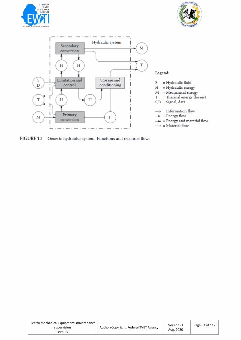
Electro mechanical Equipment maintenance supervision
Level-IV
Author/Copyright: Federal TVET Agency Version -1 Aug. 2020
Page 63 of 117

Electro mechanical Equipment maintenance supervision
Level-IV
Author/Copyright: Federal TVET Agency Version -1 Aug. 2020
Page 64 of 117
Self-Check -1 Written Test
Directions: Answer all the questions listed below. Use the Answer sheet provided in the next
page:
1. Explain about open channel?
2. What is the difference b/n pipe and channel?
3. What is hydraulic jump ?
Part two Directions: Answer all the questions listed below. Use the Answer sheet provided in the next
page
1. Write the difrence b/n water haydrolic?
2. Define haydrolic?
Electro mechanical Equipment maintenance supervision
Level-IV
Author/Copyright: Federal TVET Agency Version -1 Aug. 2020
Page 65 of 117
Flow classification
Recalling that flow may be steady or unsteady and uniform or non-uniform, the major
classifications applied to open channels are as follows:
Steady and Unsteady: Time is the criterion. Flow is said to be steady if the depth of flow at a
particular point does not change or can be considered constant for the time interval under
consideration. The flow is unsteady if depth changes with time.
Uniform and non-uniform Flow: Space as the criterion. Open Channel flow is said to be
uniform if the depth and velocity of flow are the same at every section of the channel. Hence it
follows that uniform flow can only occur in prismatic channels. Flow in channels is termed as
non-uniform or varied if the depth of flow y, changes from section to section
Non-uniform flow is rapidly varied flow If the depth of flow changes a abruptly over a
comparatively short distance; eg. Hydraulic Jump Non-Uniform flow is gradually varied flow. If
the change in depth of flow takes place gradually in a long reach of the channel.
Steady uniform flow, in which the depth is constant, both with time and distance. This
constitutes the fundamental type of flow in an open channel in which the gravity forces are in
equilibrium with the resistance forces.
Steady non-uniform flow, in which the depth varies with distance, but not with time. The flow
may be either (a) gradually varied or (b) rapidly varied.Type (a) requires the joint application of
energy and frictional resistance equations. Type (b) requires the application of energy and
momentum principles.
Unsteady non uniform flow, in which the depth varies with both time and distance (unsteady
uniform flow is very rare). This is the most complex flow type, requiring the solution of energy,
momentum and friction equations through time. The various flow types are all shown in Figure
1.2.
Laminar and turbulent flow
Flow is said to be laminar when adjacent fluid layer, move at the same (or nearlythe same)
velocity and paths of individual fluid particles do not cross or intersect.
Information Sheet 2 Hydraulics Flow
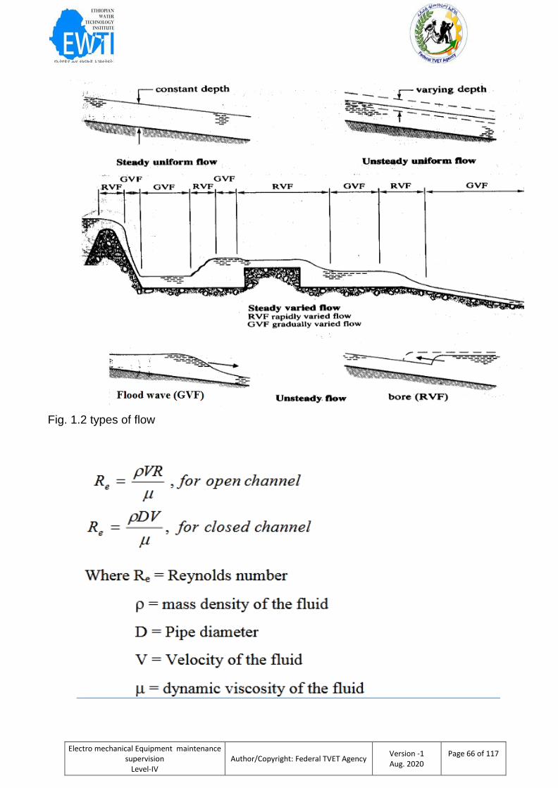
Electro mechanical Equipment maintenance supervision
Level-IV
Author/Copyright: Federal TVET Agency Version -1 Aug. 2020
Page 66 of 117
Fig. 1.2 types of flow
Electro mechanical Equipment maintenance supervision
Level-IV
Author/Copyright: Federal TVET Agency Version -1 Aug. 2020
Page 67 of 117
Critical and supercritical flow Gravity is a predominant force in the case of channel flow. As
such depending on the relative effect of gravity the inertia forces, the channel flow may be
designed as sub critical, critical or super critical. Determination of such flow depend on the
dimensionless parameter called fraud number (Fr) which is defined as the ratio of inertia the
gravity forces.

Electro mechanical Equipment maintenance supervision
Level-IV
Author/Copyright: Federal TVET Agency Version -1 Aug. 2020
Page 68 of 117
Self-Check -2 Written Test
Directions: Answer all the questions listed below. Use the Answer sheet provided in the next
page:
7. What are the classification of open channel?
8. Write the equation for fraud number?
9. What are equation used to calculate Reynolds number ?
A. In open channel
B. In cloth channel
Electro mechanical Equipment maintenance supervision
Level-IV
Author/Copyright: Federal TVET Agency Version -1 Aug. 2020
Page 69 of 117
Flow Measurement In Open Channels
Open channel flow is flow in any channel in which the liquid flows with a free surface. Included
are tunnels, partially filled pipes, canals, streams, and rivers. There are many methods of
determining the rate of flow in open channels. Some of the more common include the timed
gravimetric, dilution, velocity-area, hydraulic structures, and slope-hydraulic radius-area
methods.
Timed Gravimetric Method The flow rate is calculated by weighing the entire content of the
flow stream that was collected in a container for a fixed length of time. This is practical for small
streams of less than 25 to 30 gallons per minutes (gpm) and is not well suited for continuous
measurement.
Dilution Method The flow rate is measured by determining how much the flowing water dilutes
an added tracer solution.
Velocity-Area Method Measuring the mean flow velocity across a cross section and
multiplying it by the area at that point to calculate the flow rate.
Hydraulic Structure Method This method uses a hydraulic structure placed in the flow stream
of the channel to produce flow properties that are characterized by known relationships between
the water level measurement at some location and the flow rate of the stream. Therefore, the
flow rate is determined by taking a single measurement of the water surface level in or near the
restriction of the hydraulic structure.
Slope-hydraulic Radius-Area Method Measurement of water surface slope, cross-sectional
area, and wetted perimeter over a length of uniform section channel are used to calculate the
flow rate, by using a resistant equation such as the Manning formula.
The Gravitational, Dilution, and the Velocity Area methods are more commonly used for
calibration purposes. The Depth-Related methods (Hydraulic Structures) are the most common.
The depth-related technique measures flow rate from a measurement of the water depth, or
head. Weir and flumes are the oldest and most common devices used for measuring open
channel flows
Information Sheet 3 Methods used for measuring flows

Electro mechanical Equipment maintenance supervision
Level-IV
Author/Copyright: Federal TVET Agency Version -1 Aug. 2020
Page 70 of 117
Self-Check -3 Written Test
Directions: Answer all the questions listed below. Use the Answer sheet provided in the next
page:
Explain about measuring flows in open channel?
What different types of measuring method?
Which one is the most common method?
Electro mechanical Equipment maintenance supervision
Level-IV
Author/Copyright: Federal TVET Agency Version -1 Aug. 2020
Page 71 of 117
Introduction
An open channel is a duct in which the liquid flows with a free surface. This is in
contrast with pipe flow in which the liquid completely fills the pipe and flow under
pressure. The flow in a pipe takes place due to difference of pressure (pressure
gradient), whereas in open channel it is due to the slope of the channel bed (i.e.;
due to gravity). It may be noted that the flow in a closed conduit is not necessarily a
pipe flow. It must be classified as open channel flow if the liquid has a free surface.
Information Sheet 4 Open channel
Electro mechanical Equipment maintenance supervision
Level-IV
Author/Copyright: Federal TVET Agency Version -1 Aug. 2020
Page 72 of 117
Introduction
Channels where flow occurs under free surface can either be
4. natural, such as rivers and
5. streams, or artificial. Artificial
channels comprise all man-made channels, including irrigation and navigation canals, spillway
channels, sewers, culverts and drainage ditches. They are normally of regular cross-sectional
shape and bed slope, and as such are termed prismatic channels. Their construction materials
are varied, but commonly used materials include concrete, steel and earth. The surface
roughness characteristics of these materials are normally well defined within engineering
tolerances. In consequence, the application of hydraulic theories to flow in artificial channels will
normally yield reasonably accurate results. Various terms are used to refer to channels built
under different conditions. Canal: a channel built on ground, i.e excavated to the desired shape
and slope with or without lining, usually having a mild slope. The lining could be made of
concrete, stone masonry, cement, wood or bituminous material. Flume: a channel built (or
supported) above the ground to convey fluid from one point to another. In the field flumes are
made of concrete, wood, sheet metal or masonry. Laboratory flumes are usually made of wood,
metal, glass or a composite of these materials. Chute: is a channel of steep slopes. If the change
in elevation in the direction of flow occurs in a relatively short distance the channel is called a
drop.Culvert:is a relatively short and usually buried conduit that is commonly used for drainage
purposes, as in highways and embankments. Open channel prevails whenever the culvert is
flowing partially full.In contrast, natural channels are normally very irregular in shape, and their
materials are diverse. The surface roughness of natural channels changes with time, distance
and water surface elevation. Therefore, it is more difficult to apply hydraulic theory to natural
channels and obtain satisfactory results. Many applications involve man-made alterations to
natural channels (e.g. river control structures and flood alleviation measures). Such applications
require an understanding not only of hydraulic theory, but also of the associated disciplines of
sediment transport, hydrology and river morphology. Various geometric properties of natural and
artificial channels need to be determined for hydraulic purposes. In the case of artificial
Information Sheet 5 Types Open channel
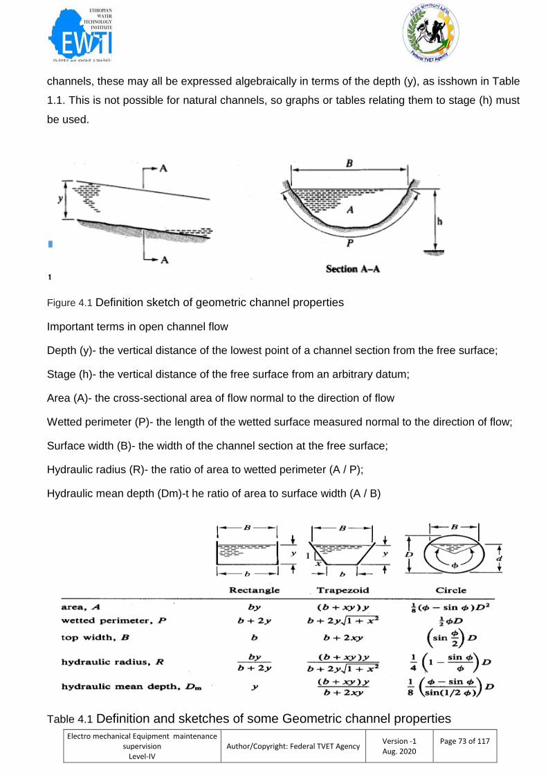
Electro mechanical Equipment maintenance supervision
Level-IV
Author/Copyright: Federal TVET Agency Version -1 Aug. 2020
Page 73 of 117
channels, these may all be expressed algebraically in terms of the depth (y), as isshown in Table
1.1. This is not possible for natural channels, so graphs or tables relating them to stage (h) must
be used.
Figure 4.1 Definition sketch of geometric channel properties
Important terms in open channel flow
Depth (y)- the vertical distance of the lowest point of a channel section from the free surface;
Stage (h)- the vertical distance of the free surface from an arbitrary datum;
Area (A)- the cross-sectional area of flow normal to the direction of flow
Wetted perimeter (P)- the length of the wetted surface measured normal to the direction of flow;
Surface width (B)- the width of the channel section at the free surface;
Hydraulic radius (R)- the ratio of area to wetted perimeter (A / P);
Hydraulic mean depth (Dm)-t he ratio of area to surface width (A / B)
Table 4.1 Definition and sketches of some Geometric channel properties
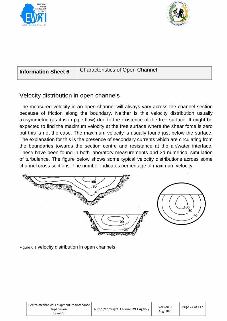
Electro mechanical Equipment maintenance supervision
Level-IV
Author/Copyright: Federal TVET Agency Version -1 Aug. 2020
Page 74 of 117
Velocity distribution in open channels
The measured velocity in an open channel will always vary across the channel section
because of friction along the boundary. Neither is this velocity distribution usually
axisymmetric (as it is in pipe flow) due to the existence of the free surface. It might be
expected to find the maximum velocity at the free surface where the shear force is zero
but this is not the case. The maximum velocity is usually found just below the surface.
The explanation for this is the presence of secondary currents which are circulating from
the boundaries towards the section centre and resistance at the air/water interface.
These have been found in both laboratory measurements and 3d numerical simulation
of turbulence. The figure below shows some typical velocity distributions across some
channel cross sections. The number indicates percentage of maximum velocity
Figure 6.1 velocity distribution in open channels
Information Sheet 6 Characteristics of Open Channel

Electro mechanical Equipment maintenance supervision
Level-IV
Author/Copyright: Federal TVET Agency Version -1 Aug. 2020
Page 75 of 117
Self-Check -6 Written Test
Directions: Answer all the questions listed below. Use the Answer sheet provided in the next
page:
1, Explain about open channel?
2, What are types of openchannel?
3, What is the difference b/n pipe and channel?
4, What is hydraulic jump ?
Note: Satisfactory rating – 30 points Unsatisfactory - below 25 points
You can ask you teacher for the copy of the correct answers
Answer Sheet
Name: _________________________ Date: _______________
Short Answer Questions
1. ____________________________________________________________________________
____________________________________________________________________________
Score =
___________
Rating:
___________
_
Electro mechanical Equipment maintenance supervision
Level-IV
Author/Copyright: Federal TVET Agency Version -1 Aug. 2020
Page 76 of 117
2. ____________________________________________________________________________
____________________________________________________________________________
_____________________________________________________________________
3. ______________________________________________________________________
_______________________________________________________________
4. ______________________________________________________________________
____________________________________________________________________
This learning guide is developed to provide you the necessary information regarding the
following content coverage and topics:
Notches and weirs
Calculating flows in notches and weirs
Characteristics of notches and weirs
Measuring instruments and devices for notches and weirs
Types of meters
Limitations of the meters
This guide will also assist you to attain the learning outcome stated in the cover page.
Specifically, upon completion of this Learning Guide, you will be able to:
. The methods used for measuring flows in notches and weirs are identified.
The formulae are used for calculating flows in notches and weirs.
The applications and characteristics of notches and weirs are distinguished.
The uses of different measuring instruments and devices used for notches and weirs are distinguished.
The hydraulic principles which apply to different meters are assessed.
The limitations of the meters are identified. Learning Instructions:
2.2. Read the specific objectives of this Learning Guide.
2.3. Follow the instructions described below
Instruction Sheet 4 Learning Guide 45: Calculate flows through notches
and weirs
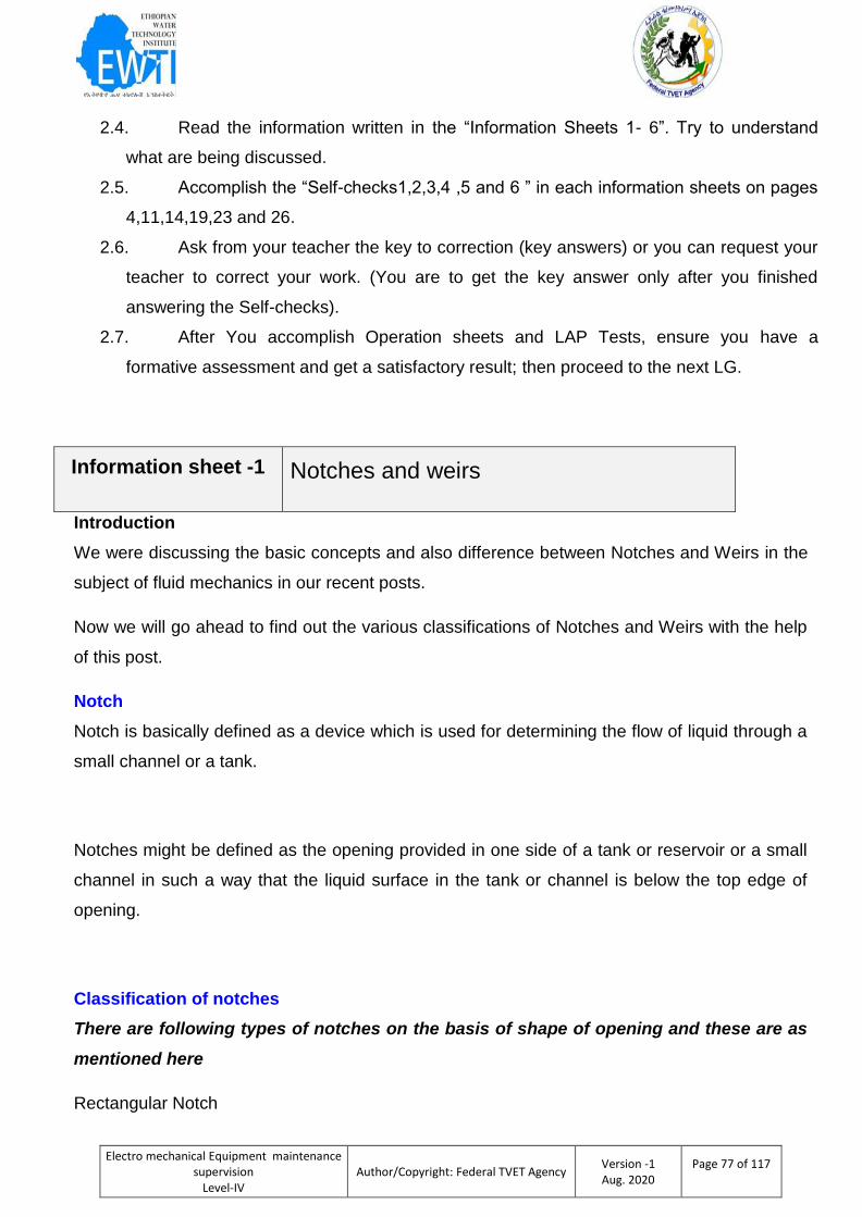
Electro mechanical Equipment maintenance supervision
Level-IV
Author/Copyright: Federal TVET Agency Version -1 Aug. 2020
Page 77 of 117
2.4. Read the information written in the “Information Sheets 1- 6”. Try to understand
what are being discussed.
2.5. Accomplish the “Self-checks1,2,3,4 ,5 and 6 ” in each information sheets on pages
4,11,14,19,23 and 26.
2.6. Ask from your teacher the key to correction (key answers) or you can request your
teacher to correct your work. (You are to get the key answer only after you finished
answering the Self-checks).
2.7. After You accomplish Operation sheets and LAP Tests, ensure you have a
formative assessment and get a satisfactory result; then proceed to the next LG.
Information sheet -1 Notches and weirs
Introduction
We were discussing the basic concepts and also difference between Notches and Weirs in the
subject of fluid mechanics in our recent posts.
Now we will go ahead to find out the various classifications of Notches and Weirs with the help
of this post.
Notch
Notch is basically defined as a device which is used for determining the flow of liquid through a
small channel or a tank.
Notches might be defined as the opening provided in one side of a tank or reservoir or a small
channel in such a way that the liquid surface in the tank or channel is below the top edge of
opening.
Classification of notches
There are following types of notches on the basis of shape of opening and these are as
mentioned here
Rectangular Notch
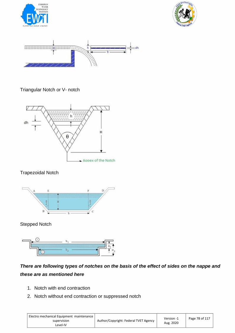
Electro mechanical Equipment maintenance supervision
Level-IV
Author/Copyright: Federal TVET Agency Version -1 Aug. 2020
Page 78 of 117
Triangular Notch or V- notch
Trapezoidal Notch
Stepped Notch
There are following types of notches on the basis of the effect of sides on the nappe and
these are as mentioned here
1. Notch with end contraction
2. Notch without end contraction or suppressed notch
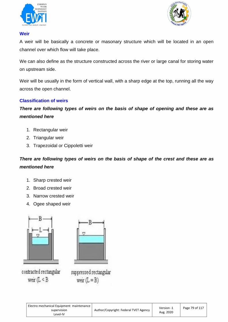
Electro mechanical Equipment maintenance supervision
Level-IV
Author/Copyright: Federal TVET Agency Version -1 Aug. 2020
Page 79 of 117
Weir
A weir will be basically a concrete or masonary structure which will be located in an open
channel over which flow will take place.
We can also define as the structure constructed across the river or large canal for storing water
on upstream side.
Weir will be usually in the form of vertical wall, with a sharp edge at the top, running all the way
across the open channel.
Classification of weirs
There are following types of weirs on the basis of shape of opening and these are as
mentioned here
1. Rectangular weir
2. Triangular weir
3. Trapezoidal or Cippoletti weir
There are following types of weirs on the basis of shape of the crest and these are as
mentioned here
1. Sharp crested weir
2. Broad crested weir
3. Narrow crested weir
4. Ogee shaped weir
Electro mechanical Equipment maintenance supervision
Level-IV
Author/Copyright: Federal TVET Agency Version -1 Aug. 2020
Page 80 of 117
There are following types of weirs on the basis of the effect of sides on the emerging
nappe and these are as mentioned here
1. Weirs with end contraction
2. Weirs without end contraction or suppressed notch
Self-Check -1 Written Test
Direction : answer the following questions
1. What is Notch?
2. What is weir?
3. What is the different between notches and weirs?
4. Write classification of weirs?
5. Write classification of notches?
Electro mechanical Equipment maintenance supervision
Level-IV
Author/Copyright: Federal TVET Agency Version -1 Aug. 2020
Page 81 of 117
Information sheet-2 formulae are used for calculating flows in notches and weirs
Introduction
A notch means an opening provided in the side of a tank, such that the opening extends even above the
free surface of the liquid in the tank. It is in a way, a large orifice having no upper edge. A notch is
generally meant to measure the flow of water from a tank. A weir is also a notch but it is made on a large
scale. The weir is a notch cut in a dam to discharge the surplus quantity of water.
Water flows over a notch or weir while water passes through an orifice. While the stream of water
discharged by an orifice is called a jet, the sheet of water discharged by a notch or weir is called a nappe
or vein. The upper surface of the notch or weir over which the water flows is called the Crest or Sill
A notch or a weir is a convenient device for the measurement of discharge in an open channel. A notch
or a weir is an obstruction provided in a channel that causes the water to rise behind it so that the water is
made to flow through it or over it. The rate of flow can be determined by measuring the height of the
upstream water level.
Basically there is no difference between a notch and a weir, except that a notch is of small size while a
weir is of large size. A notch is usually made of metal plate whereas a weir is made of masonry or
concrete.
1.1 Calculating Notches
Notch is basically defined as a device which is used for determining the flow of liquid through a small channel or
a tank. Notches might be defined as the opening provided in one side of a tank or reservoir or a small channel in
such a way that the liquid surface in the tank or channel is below the top edge of opening.
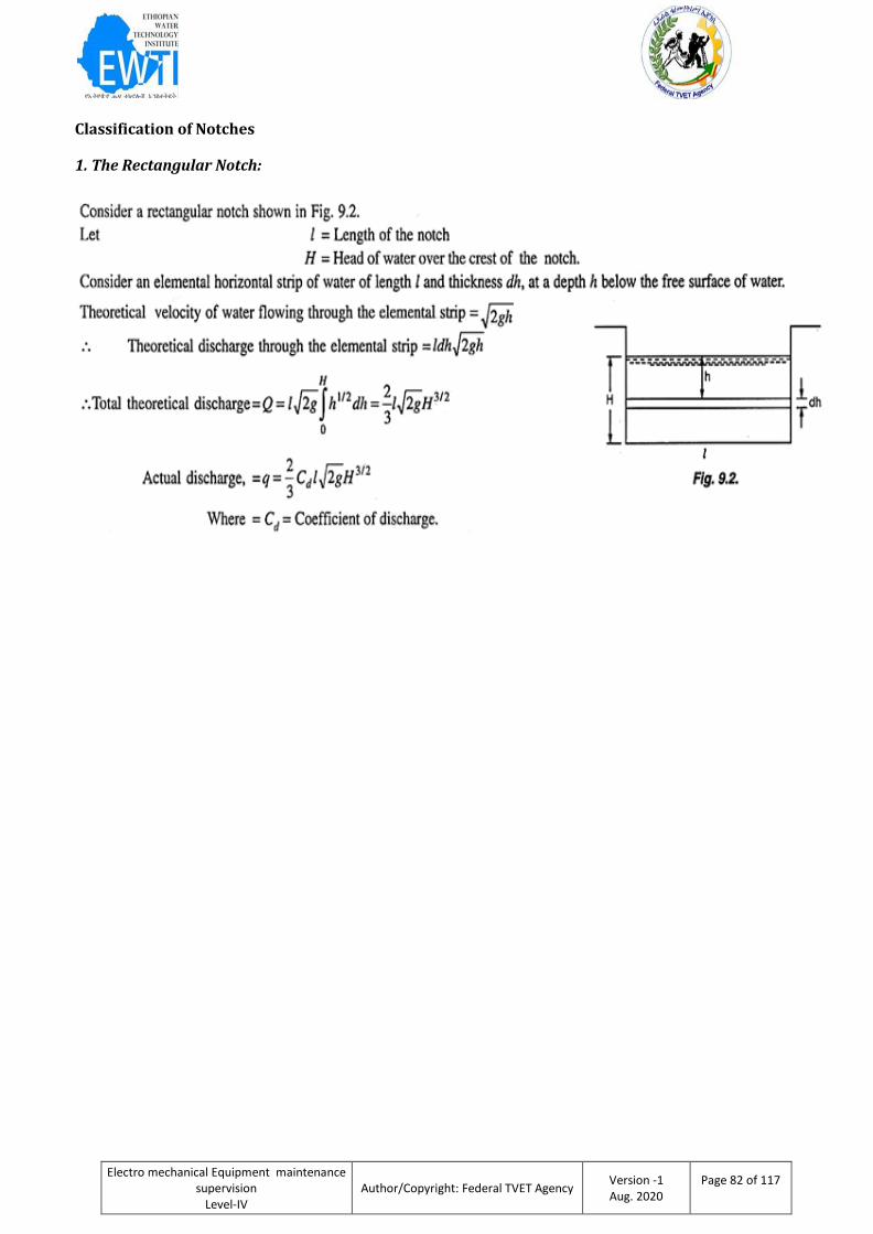
Electro mechanical Equipment maintenance supervision
Level-IV
Author/Copyright: Federal TVET Agency Version -1 Aug. 2020
Page 82 of 117
Classification of Notches
1. The Rectangular Notch:
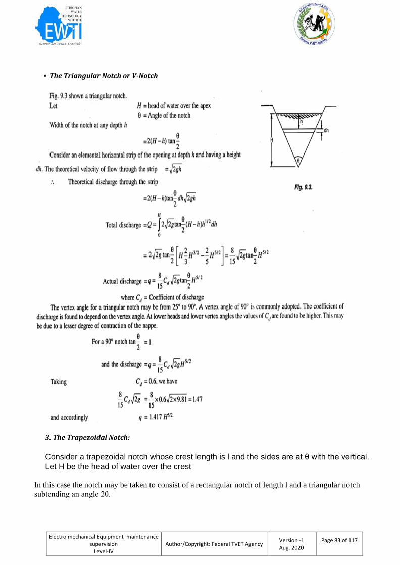
Electro mechanical Equipment maintenance supervision
Level-IV
Author/Copyright: Federal TVET Agency Version -1 Aug. 2020
Page 83 of 117
The Triangular Notch or V-Notch
3. The Trapezoidal Notch:
Consider a trapezoidal notch whose crest length is l and the sides are at θ with the vertical. Let H be the head of water over the crest
In this case the notch may be taken to consist of a rectangular notch of length l and a triangular notch
subtending an angle 2θ.
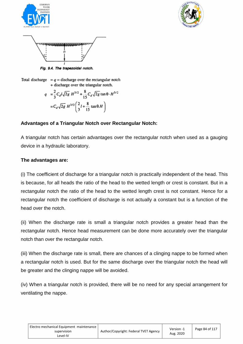
Electro mechanical Equipment maintenance supervision
Level-IV
Author/Copyright: Federal TVET Agency Version -1 Aug. 2020
Page 84 of 117
Advantages of a Triangular Notch over Rectangular Notch:
A triangular notch has certain advantages over the rectangular notch when used as a gauging
device in a hydraulic laboratory.
The advantages are:
(i) The coefficient of discharge for a triangular notch is practically independent of the head. This
is because, for all heads the ratio of the head to the wetted length or crest is constant. But in a
rectangular notch the ratio of the head to the wetted length crest is not constant. Hence for a
rectangular notch the coefficient of discharge is not actually a constant but is a function of the
head over the notch.
(ii) When the discharge rate is small a triangular notch provides a greater head than the
rectangular notch. Hence head measurement can be done more accurately over the triangular
notch than over the rectangular notch.
(iii) When the discharge rate is small, there are chances of a clinging nappe to be formed when
a rectangular notch is used. But for the same discharge over the triangular notch the head will
be greater and the clinging nappe will be avoided.
(iv) When a triangular notch is provided, there will be no need for any special arrangement for
ventilating the nappe.
Electro mechanical Equipment maintenance supervision
Level-IV
Author/Copyright: Federal TVET Agency Version -1 Aug. 2020
Page 85 of 117
1.2 Calculating Weir
A weir will be basically a concrete or masonary structure which will be located in an open
channel over which flow will take place. We can also define as the structure constructed across
the river or large canal for storing water on upstream side. Weir will be usually in the form of
vertical wall, with a sharp edge at the top, running all the way across the open channel. Weirs
are common and simple methods of measuring the flow of water in open channels. At its
simplest, a weir is no more than an obstruction placed in a channel over which water flows
(unlike flumes where the water flows through the structure). Often this flow is over a specially
shaped notch or opening set above the floor of the channel.
Properly size, built, and maintained, a weir can provide inexpensive and accurate flow
measurements.
Open channel flow offers a variety of weirs, including: fixed weir plates, portable weir sets, weir
boxes, weir channels, and weir manholes.
Classification of Weirs:
1. Proportional Weir:
This is a weir whose shape is so designed that the discharge over the weir is proportional to the head of
water over the crest. The crest of the weir is horizontal.
Consider the weir shown in Fig. 9.13, whose equation with the middle point of the crest as origin is x2 =
K/y where K is a constant. Let H be the head of water over the weir. Consider a horizontal strip of the
flow section of width 2x at a height y above the crest. Let dy be the thickness of the strip. Discharge
through the elemental horizontal strip.
Electro mechanical Equipment maintenance supervision
Level-IV
Author/Copyright: Federal TVET Agency Version -1 Aug. 2020
Page 86 of 117
2. The Cippoletti Weir:
We know for a rectangular weir with the two end contractions, the discharge is given by –
3. Submerged Weir:
Fig. 9.19 shows a submerged weir. In this case the water level on the downstream side also is above the crest of the weir. Let H1 and H2 be the heights of the upstream and downstream water levels above the crest weir. The total discharge Q consists of components Q1 and Q2.
4. Anicut or Raised Weir or Barrage:
An anicut is a masonry dam provided across a river for the purpose of raising the water level on the upstream side to a sufficient extent in the dry season, so that the water can be carried by gravitation to places where it otherwise could not reach.
Time of Emptying a Reservoir by a Rectangular Weir:
Let a reservoir of plan area A be provided with a rectangular weir of length I. Let it be required to find the time taken for the head of water over the weir to fall from a value H1 to a value H2.
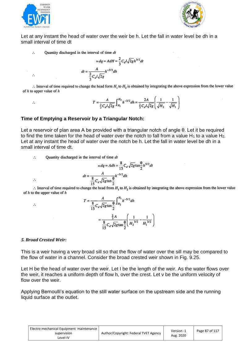
Electro mechanical Equipment maintenance supervision
Level-IV
Author/Copyright: Federal TVET Agency Version -1 Aug. 2020
Page 87 of 117
Let at any instant the head of water over the weir be h. Let the fall in water level be dh in a small interval of time dt
Time of Emptying a Reservoir by a Triangular Notch:
Let a reservoir of plan area A be provided with a triangular notch of angle θ. Let it be required to find the time taken for the head of water over the notch to fall from a value H1 to a value H2. Let at any instant the head of water over the notch be h. Let the fall in water level be dh in a small interval of time dt.
5. Broad Crested Weir:
This is a weir having a very broad sill so that the flow of water over the sill may be compared to the flow of water in a channel. Consider the broad crested weir shown in Fig. 9.25.
Let H be the head of water over the weir. Let I be the length of the weir. As the water flows over the weir, it reaches a uniform depth of flow h, over the crest. Let v be the uniform velocity of flow over the weir.
Applying Bernoulli’s equation to the still water surface on the upstream side and the running liquid surface at the outlet.
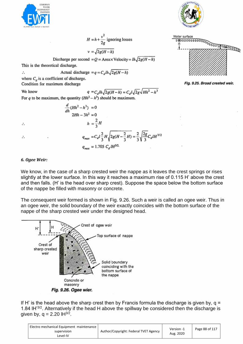
Electro mechanical Equipment maintenance supervision
Level-IV
Author/Copyright: Federal TVET Agency Version -1 Aug. 2020
Page 88 of 117
6. Ogee Weir:
We know, in the case of a sharp crested weir the nappe as it leaves the crest springs or rises slightly at the lower surface. In this way it reaches a maximum rise of 0.115 H’ above the crest and then falls. (H’ is the head over sharp crest). Suppose the space below the bottom surface of the nappe be filled with masonry or concrete.
The consequent weir formed is shown in Fig. 9.26. Such a weir is called an ogee weir. Thus in an ogee weir, the solid boundary of the weir exactly coincides with the bottom surface of the nappe of the sharp crested weir under the designed head.
If H’ is the head above the sharp crest then by Francis formula the discharge is given by, q = 1.84 lH’3/2. Alternatively if the head H above the spillway be considered then the discharge is given by, q = 2.20 lH3/2.

Electro mechanical Equipment maintenance supervision
Level-IV
Author/Copyright: Federal TVET Agency Version -1 Aug. 2020
Page 89 of 117
7. Separating Weir:
A separating weir is an arrangement provided in the case of town water supply, where it may become necessary to divert the discoloured flood water from the supply channel. When the discharge is moderate, the water drops over the lip C into a culvert D which communicates with the supply channel.
But during floods, the velocity of flow will be greater due to greater depth and this causes the water to leap across the opening into the waste channel.
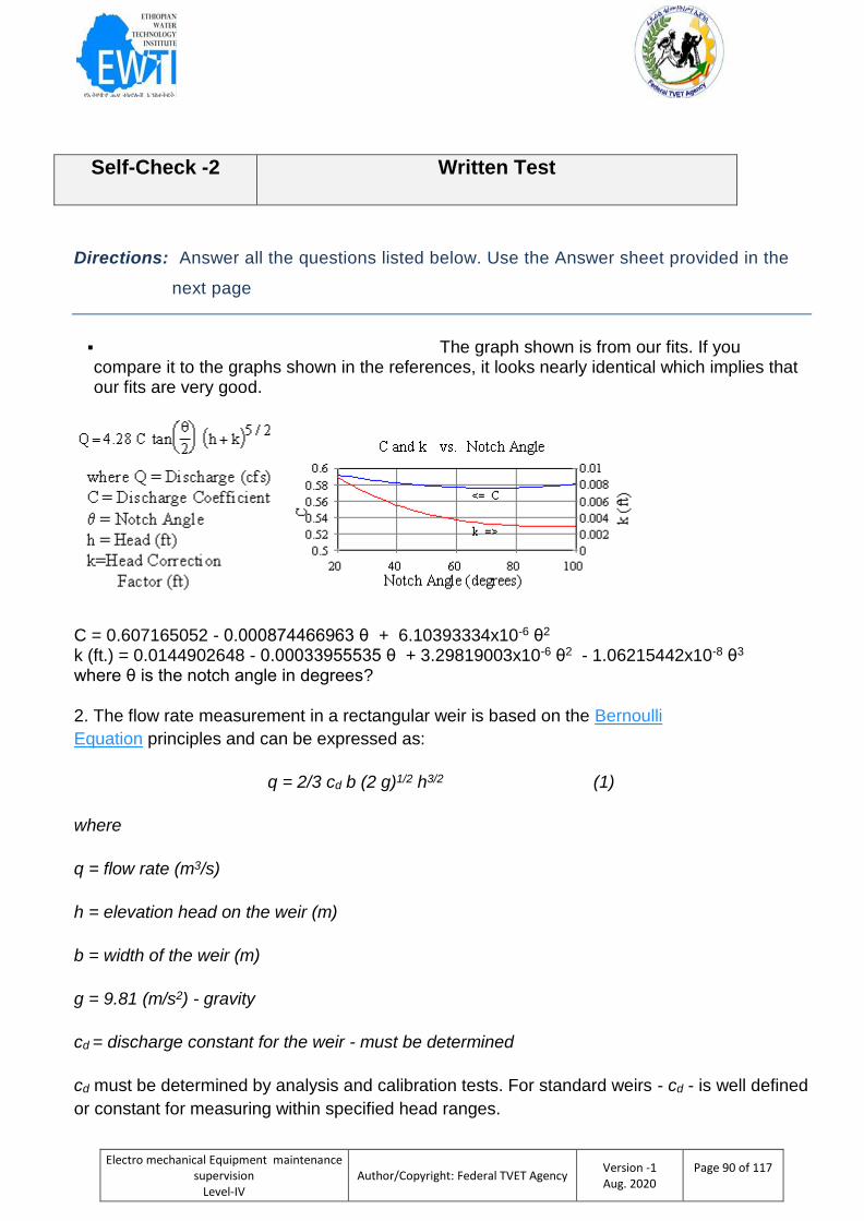
Electro mechanical Equipment maintenance supervision
Level-IV
Author/Copyright: Federal TVET Agency Version -1 Aug. 2020
Page 90 of 117
Self-Check -2 Written Test
Directions: Answer all the questions listed below. Use the Answer sheet provided in the
next page
The graph shown is from our fits. If you compare it to the graphs shown in the references, it looks nearly identical which implies that our fits are very good.
C = 0.607165052 - 0.000874466963 θ + 6.10393334x10⁻⁶ θ2 k (ft.) = 0.0144902648 - 0.00033955535 θ + 3.29819003x10⁻⁶ θ2 - 1.06215442x10⁻⁸ θ3 where θ is the notch angle in degrees?
2. The flow rate measurement in a rectangular weir is based on the Bernoulli
Equation principles and can be expressed as:
q = 2/3 cd b (2 g)1/2 h3/2 (1)
where
q = flow rate (m3/s)
h = elevation head on the weir (m)
b = width of the weir (m)
g = 9.81 (m/s2) - gravity
cd = discharge constant for the weir - must be determined
cd must be determined by analysis and calibration tests. For standard weirs - cd - is well defined
or constant for measuring within specified head ranges.
Electro mechanical Equipment maintenance supervision
Level-IV
Author/Copyright: Federal TVET Agency Version -1 Aug. 2020
Page 91 of 117
The lowest elevation (h = 0) of the overflow opening of the sharp-crested weirs or the control
channel of broad-
The characteristics of weirs
They have different in a shape also the applications’ for example
Sharp-Crested Weirs
Sharp-crested weirs are typically constructed by placing a thin, rust resistant metal plate, with a
notch in the top of it, perpendicular to the flow of water (concrete and timber can also be used
to construct). Water will flow through the notch and the depth of water that flows through it will
correlate to the discharge in the channel (Cruise). There are three main types of sharp-crested
weirs: rectangular, triangular, and trapezoidal
Rectangular Weirs -
Rectangular weirs are typically used to control the elevation of water up and downstream of
the weir and they usually have higher discharge values associated with them. There are two
main types of rectangular weirs. The first type is a suppressed weir, where the crest stretches
across the whole width of the channel
Information Sheet 3 characteristics of notches and weirs
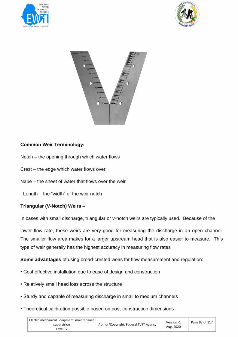
Electro mechanical Equipment maintenance supervision
Level-IV
Author/Copyright: Federal TVET Agency Version -1 Aug. 2020
Page 92 of 117
Common Weir Terminology:
Notch – the opening through which water flows
Crest – the edge which water flows over
Nape – the sheet of water that flows over the weir
Length – the “width” of the weir notch
Triangular (V-Notch) Weirs –
In cases with small discharge, triangular or v-notch weirs are typically used. Because of the
lower flow rate, these weirs are very good for measuring the discharge in an open channel.
The smaller flow area makes for a larger upstream head that is also easier to measure. This
type of weir generally has the highest accuracy in measuring flow rates
Some advantages of using broad-crested weirs for flow measurement and regulation:
• Cost effective installation due to ease of design and construction
• Relatively small head loss across the structure
• Sturdy and capable of measuring discharge in small to medium channels
• Theoretical calibration possible based on post-construction dimensions
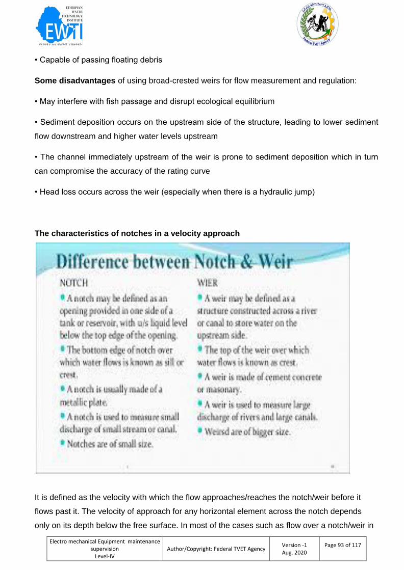
Electro mechanical Equipment maintenance supervision
Level-IV
Author/Copyright: Federal TVET Agency Version -1 Aug. 2020
Page 93 of 117
• Capable of passing floating debris
Some disadvantages of using broad-crested weirs for flow measurement and regulation:
• May interfere with fish passage and disrupt ecological equilibrium
• Sediment deposition occurs on the upstream side of the structure, leading to lower sediment
flow downstream and higher water levels upstream
• The channel immediately upstream of the weir is prone to sediment deposition which in turn
can compromise the accuracy of the rating curve
• Head loss occurs across the weir (especially when there is a hydraulic jump)
The characteristics of notches in a velocity approach
It is defined as the velocity with which the flow approaches/reaches the notch/weir before it
flows past it. The velocity of approach for any horizontal element across the notch depends
only on its depth below the free surface. In most of the cases such as flow over a notch/weir in
Electro mechanical Equipment maintenance supervision
Level-IV
Author/Copyright: Federal TVET Agency Version -1 Aug. 2020
Page 94 of 117
the side of the reservoir, the velocity of approach may be neglected. But, for the notch/weir
placed at the end of the narrow channel, the velocity of approach to the weir will be substantial
and the head producing the flow will be increased by the kinetic energy of the approaching
liquid. Thus, if is the velocity of approach, then the additional head due to velocity of
approach, acts on the water flowing over the notch or weir. So, the initial and final height of
water over the notch/weir will be and respectively. It may be determined by finding
the discharge over the notch/weir neglecting the velocity of approach i.e.
(1)
where Q is the discharge over the notch/weir and A is the cross-sectional area of channel
on the upstream side of the weir/notch. V Additional head corresponding to the velocity of
approach will be
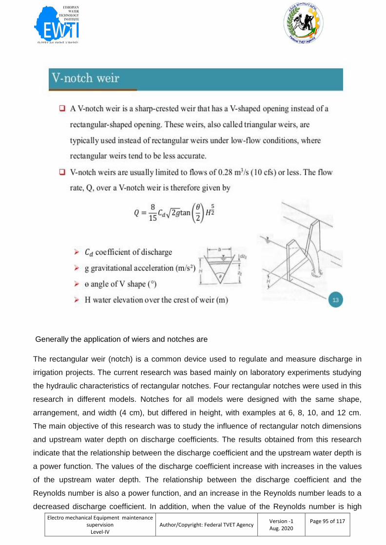
Electro mechanical Equipment maintenance supervision
Level-IV
Author/Copyright: Federal TVET Agency Version -1 Aug. 2020
Page 95 of 117
Generally the application of wiers and notches are
The rectangular weir (notch) is a common device used to regulate and measure discharge in
irrigation projects. The current research was based mainly on laboratory experiments studying
the hydraulic characteristics of rectangular notches. Four rectangular notches were used in this
research in different models. Notches for all models were designed with the same shape,
arrangement, and width (4 cm), but differed in height, with examples at 6, 8, 10, and 12 cm.
The main objective of this research was to study the influence of rectangular notch dimensions
and upstream water depth on discharge coefficients. The results obtained from this research
indicate that the relationship between the discharge coefficient and the upstream water depth is
a power function. The values of the discharge coefficient increase with increases in the values
of the upstream water depth. The relationship between the discharge coefficient and the
Reynolds number is also a power function, and an increase in the Reynolds number leads to a
decreased discharge coefficient. In addition, when the value of the Reynolds number is high

Electro mechanical Equipment maintenance supervision
Level-IV
Author/Copyright: Federal TVET Agency Version -1 Aug. 2020
Page 96 of 117
(turbulent flow), the values of the discharge coefficient converge to an approximately constant
value. The flow in all runs was subcritical and the relationship between discharge coefficient
and Froude number was also found to be a power function. An increase in Froude number thus
leads to a decrease in discharge coefficient. The slope of the discharge coefficient-Froude
number curve values gradually decreases until the value the discharge coefficient reaches an
approximately constant value. A dimensional analysis technique was used to estimate the
values of the discharge coefficient for various rectangular notch dimensions, and an empirical
equation for discharge coefficient estimating was derived using regression procedure. This
equation has a coefficient of determination R² of 0.955.
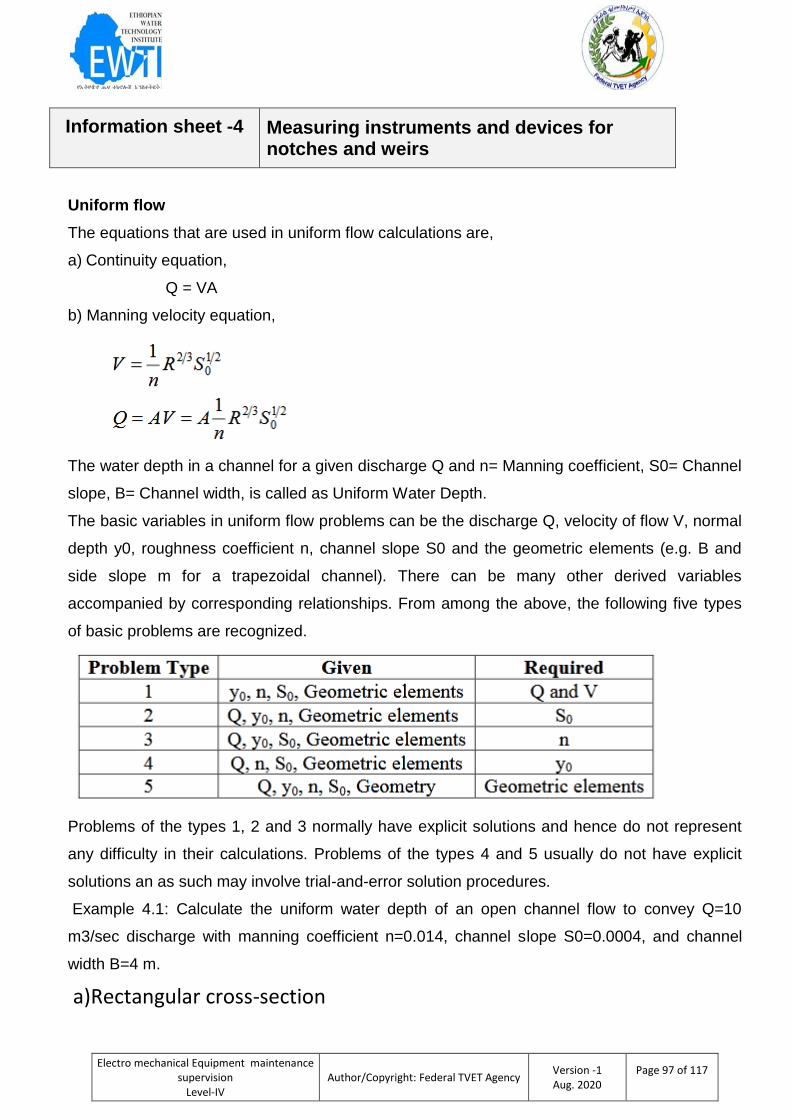
Electro mechanical Equipment maintenance supervision
Level-IV
Author/Copyright: Federal TVET Agency Version -1 Aug. 2020
Page 97 of 117
Information sheet -4 Measuring instruments and devices for notches and weirs
Uniform flow
The equations that are used in uniform flow calculations are,
a) Continuity equation,
Q = VA
b) Manning velocity equation,
The water depth in a channel for a given discharge Q and n= Manning coefficient, S0= Channel
slope, B= Channel width, is called as Uniform Water Depth.
The basic variables in uniform flow problems can be the discharge Q, velocity of flow V, normal
depth y0, roughness coefficient n, channel slope S0 and the geometric elements (e.g. B and
side slope m for a trapezoidal channel). There can be many other derived variables
accompanied by corresponding relationships. From among the above, the following five types
of basic problems are recognized.
Problems of the types 1, 2 and 3 normally have explicit solutions and hence do not represent
any difficulty in their calculations. Problems of the types 4 and 5 usually do not have explicit
solutions an as such may involve trial-and-error solution procedures.
Example 4.1: Calculate the uniform water depth of an open channel flow to convey Q=10
m3/sec discharge with manning coefficient n=0.014, channel slope S0=0.0004, and channel
width B=4 m.
a)Rectangular cross-section
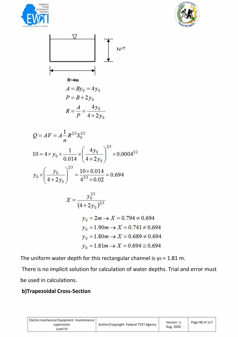
Electro mechanical Equipment maintenance supervision
Level-IV
Author/Copyright: Federal TVET Agency Version -1 Aug. 2020
Page 98 of 117
The uniform water depth for this rectangular channel is y0 = 1.81 m.
There is no implicit solution for calculation of water depths. Trial and error must
be used in calculations.
b)Trapezoidal Cross-Section
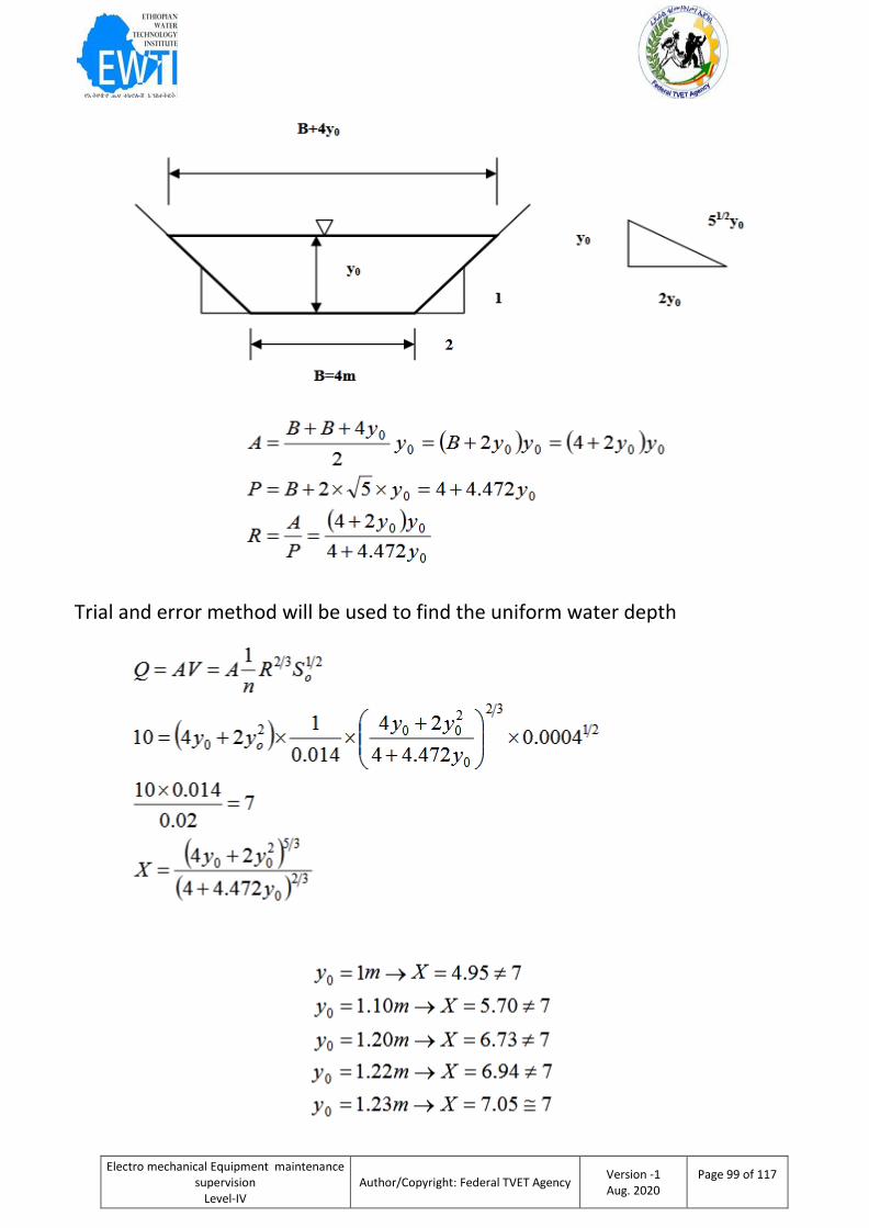
Electro mechanical Equipment maintenance supervision
Level-IV
Author/Copyright: Federal TVET Agency Version -1 Aug. 2020
Page 99 of 117
Trial and error method will be used to find the uniform water depth
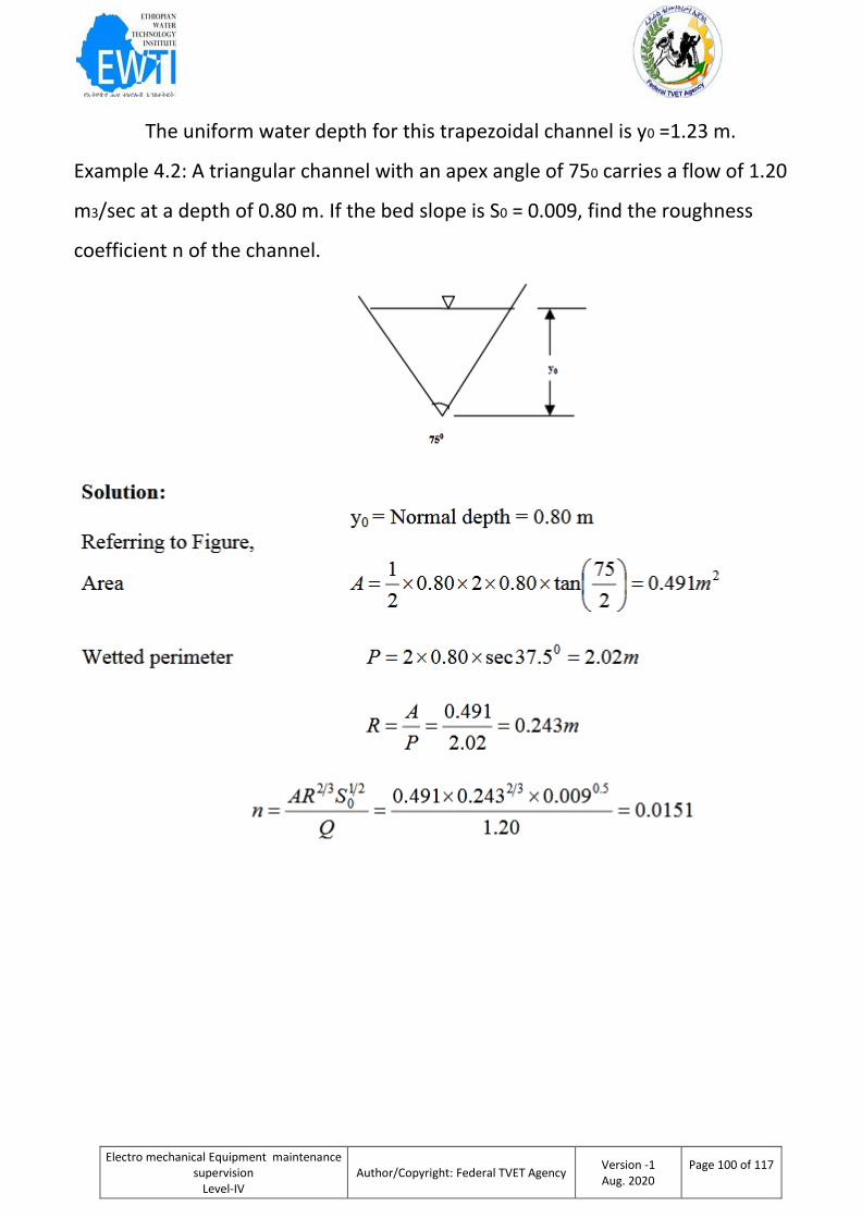
Electro mechanical Equipment maintenance supervision
Level-IV
Author/Copyright: Federal TVET Agency Version -1 Aug. 2020
Page 100 of 117
The uniform water depth for this trapezoidal channel is y0 =1.23 m.
Example 4.2: A triangular channel with an apex angle of 750 carries a flow of 1.20
m3/sec at a depth of 0.80 m. If the bed slope is S0 = 0.009, find the roughness
coefficient n of the channel.

Electro mechanical Equipment maintenance supervision
Level-IV
Author/Copyright: Federal TVET Agency Version -1 Aug. 2020
Page 101 of 117
Self-Check -4 Written Test
Directions: Answer all the questions listed below. Use the Answer sheet provided in the next
page:
2. Calculate the uniform water depth of an open channel flow to convey Q=10 m3/sec discharge with manning coefficient n=0.014, channel slope S0=0.0004, and channel width B=4 m.
3. A triangular channel with an apex angle of 750 carries a flow of 1.20 m3/sec at a depth of 0.80 m. If the bed slope is S0 = 0.009, find the roughness coefficient n of the channel.
Electro mechanical Equipment maintenance supervision
Level-IV
Author/Copyright: Federal TVET Agency Version -1 Aug. 2020
Page 102 of 117
Information sheet -5 Types of meters
CURRENT METER
A current meter is oceanographic device for flow measurement by mechanical (rotor current
meter), tilt (Tilt Current Meter), acoustical (ADCP) or electrical means.
MEASUREMENT PRINCIPLES
a. Mechanical current meters are mostly based on counting the rotations of a propeller and
are thusrotor current meters. A mid-20th-century realization is theEkman current meterwhich
drops balls into a container to count the number of rotations.
b.Acoustic There are two basic types of acoustic current meters: Doppler and Travel Time.
Both methods use a ceramic transducer to emit a sound into the water.Doppler instruments are
more common. An instrument of this type is theAcoustic Doppler Current Profiler(ADCP)which
measures the water current velocities over a depth range using theDoppler effectofsound
wavesscattered back from particles within the water column. The ADCPs use the traveling time
of the sound to determine the position of the moving particles. Single-point devices use again
the Doppler shift, but ignoring the traveling times. Such a single point Doppler Current Sensor
(DCS) has a typical velocity range of 0 to 300cm/s.Travel time instruments determine water
velocity by at least two acoustic signals, one up stream and one down stream.
c. Electromagnetic Induction This novel approach is for instance employed in the Florida
Strait where electromagnetic induction in submerged telephone cableis used to estimate the
through-flow through the gatewayand the complete setup can be seen asone huge current
meter. it is possible to evaluate the variability of the averaged horizontal flow by measuring the
induced electric currents. The method has a minor vertical weighting effect due to small
conductivity changes at different depths.
d.Tilt. current meters operate under the drag-tilt principle. They consist of a sub-surface buoy
that is anchored to the sea floor with a flexible line or tether. The float tilts as a function of its
shape, buoyancy and the water velocity. Once the characteristics of a given buoy are known,
Electro mechanical Equipment maintenance supervision
Level-IV
Author/Copyright: Federal TVET Agency Version -1 Aug. 2020
Page 103 of 117
the velocity can be determined by measuring the angle of the buoy.A Tilt Current Meter is
typically deployed on the bottom with an anchor but may be deployed on lobster traps or other
convenient anchors of opportunity.
VENTURIMETER
Venturimeter is a device used for measuring the rate of flow of a fluid flowing through a pipe. It
consists of three parts:• A short converging part
Throat Diverging partLet d1 = diameter at the inlet (section 1)p1 = pressure at section 1v1 =
velocity at section 1A1= area at section1 d2, p2, v2, A2 are the corresponding values at the
throat (section 2) Applying Bernoulli’s equations at sections 1 and 2, we get
ORIFICE METER
An orifice meter is a conduit and a restriction to create a pressure drop. An hour glass is a form
of orifice. A nozzle, venturi or thin sharp edged orifice can be used as the flow restriction. In
order to use any of these devices for measurement it is necessary to empirically calibrate them.
That is, pass a known volume through the meter and note the reading in order to provide a
standard for measuring other quantities. Due to the ease of duplicating and the simple
construction, the thin sharp edged orifice has been adopted as a standard and extensive
calibration work has been done so that it is widely accepted as a standard means of measuring
fluids.
Electro mechanical Equipment maintenance supervision
Level-IV
Author/Copyright: Federal TVET Agency Version -1 Aug. 2020
Page 104 of 117
Instruction sheet -5 Learning guide 46: Calculate proportion
for economic section
This learning guide is developed to provide you the necessary information regarding the
following content coverage and topics –
Calculating proportions of rectangular, trapezoidal and circular channels for maximum
discharge
Differentiate a partial flow chart is used to identify the depth of flow for maximum discharge
and maximum velocity
This guide will also assist you to attain the learning outcome stated in the cover page.
Specifically, upon completion of this Learning Guide, you will be able to –
Understand The proportions of rectangular, trapezoidal and circular channels are
calculated for maximum discharge.
Differentiate A partial flow chart is used to identify the depth of flow for maximum discharge
and maximum velocity
Learning Instructions
1. Read the specific objectives of this Learning Guide.
2. Follow the instructions described below
3. Read the information written in the “Information Sheets 1- 2”. Try to understand what are
being discussed.
4. Accomplish the “Self-checks1and 2 ” in each information sheets on
5. Ask from your teacher the key to correction (key answers) or you can request your
teacher to correct your work. (You are to get the key answer only after you finished
answering the Self-checks).
6. After You accomplish Operation sheets and LAP Tests, ensure you have a formative
assessment and get a satisfactory result; then proceed to the next LG.
Electro mechanical Equipment maintenance supervision
Level-IV
Author/Copyright: Federal TVET Agency Version -1 Aug. 2020
Page 105 of 117
Information sheet -1 Calculating proportions of rectangular, trapezoidal
and circular channels for maximum discharge
Introduction to Most Economical Section of Channels
A section of a channel is said to be most economical when the cost of construction of the channel is minimum. But the cost of construction of a channel depends on excavation and the lining. To keep the cost down or minimum, the wetted perimeter, for a given discharge, should be minimum. This condition is utilized for determining the dimensions of economical sections of different forms of channels. Most economical section is also called the best section or most efficient section as the discharge, passing through a most economical section of channel for a given cross-sectional area A, slope of the bed S0 and a resistance coefficient, is maximum. But the discharge
Hence the discharge Q will be maximum when the wetted perimeter P is minimum
1.1 Most Economical Rectangular Channel
Consider a rectangular section of channel as shown.
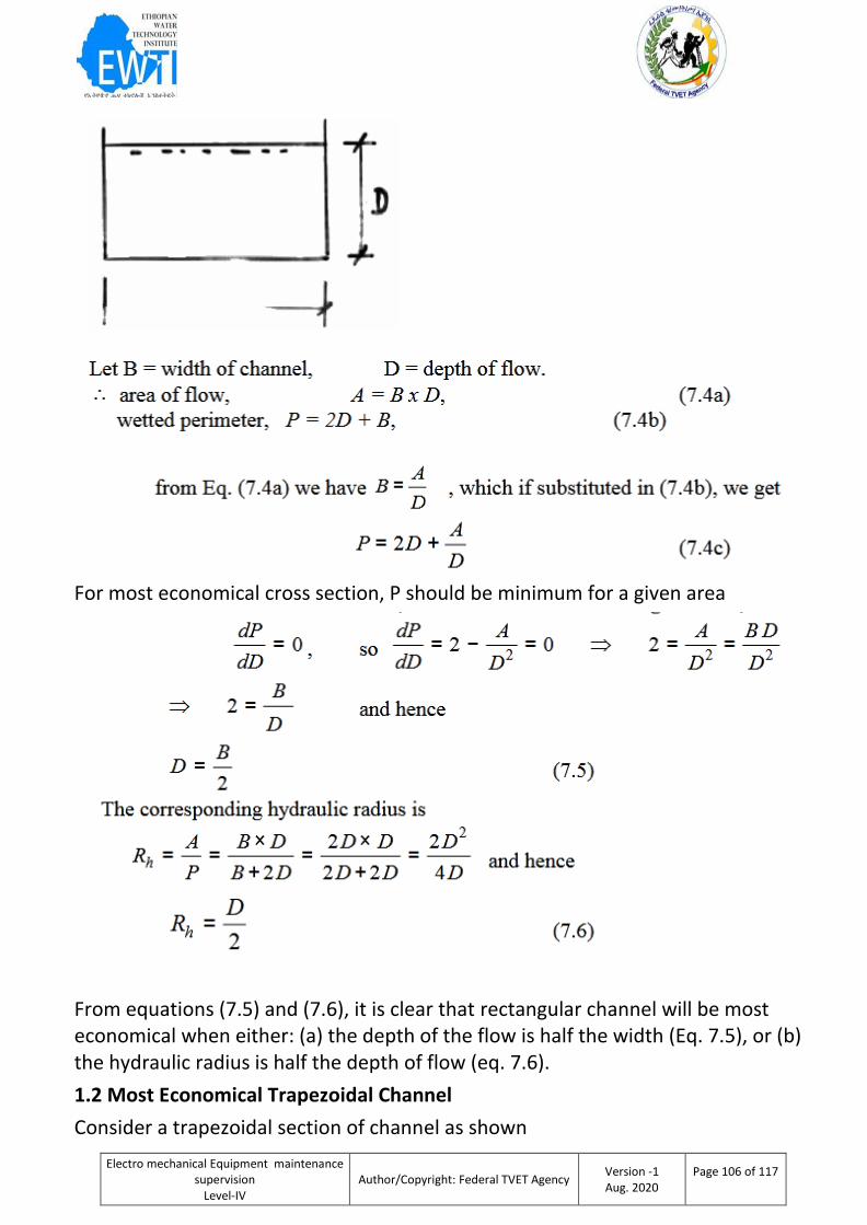
Electro mechanical Equipment maintenance supervision
Level-IV
Author/Copyright: Federal TVET Agency Version -1 Aug. 2020
Page 106 of 117
For most economical cross section, P should be minimum for a given area
From equations (7.5) and (7.6), it is clear that rectangular channel will be most economical when either: (a) the depth of the flow is half the width (Eq. 7.5), or (b) the hydraulic radius is half the depth of flow (eq. 7.6).
1.2 Most Economical Trapezoidal Channel
Consider a trapezoidal section of channel as shown
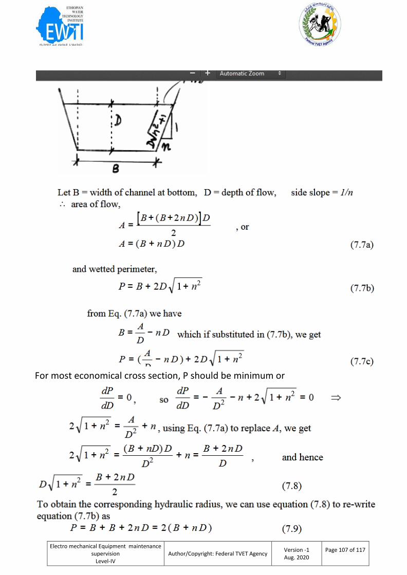
Electro mechanical Equipment maintenance supervision
Level-IV
Author/Copyright: Federal TVET Agency Version -1 Aug. 2020
Page 107 of 117
For most economical cross section, P should be minimum or
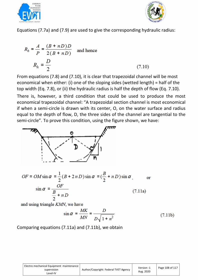
Electro mechanical Equipment maintenance supervision
Level-IV
Author/Copyright: Federal TVET Agency Version -1 Aug. 2020
Page 108 of 117
Equations (7.7a) and (7.9) are used to give the corresponding hydraulic radius:
From equations (7.8) and (7.10), it is clear that trapezoidal channel will be most economical when either: (i) one of the sloping sides (wetted length) = half of the top width (Eq. 7.8), or (ii) the hydraulic radius is half the depth of flow (Eq. 7.10).
There is, however, a third condition that could be used to produce the most economical trapezoidal channel: “A trapezoidal section channel is most economical if when a semi-circle is drawn with its center, O, on the water surface and radius equal to the depth of flow, D, the three sides of the channel are tangential to the semi-circle”. To prove this condition, using the figure shown, we have:
Comparing equations (7.11a) and (7.11b), we obtain
Electro mechanical Equipment maintenance supervision
Level-IV
Author/Copyright: Federal TVET Agency Version -1 Aug. 2020
Page 109 of 117
Thus, if a semi-circle is drawn with O as center and radius equal to the depth of
flow D, the three sides of a most economical trapezoidal section will be tangential
to the semi-circle.
Best side slope for most economical trapezoidal section can be shown to be when
So far we assumed that the side slopes are constant. Let us now consider the case when the side slopes can also vary. The most economical side slopes of a most economical trapezoidal section can be obtained as follows:
or most economical side slopes of a most efficient cross section we satisfy the
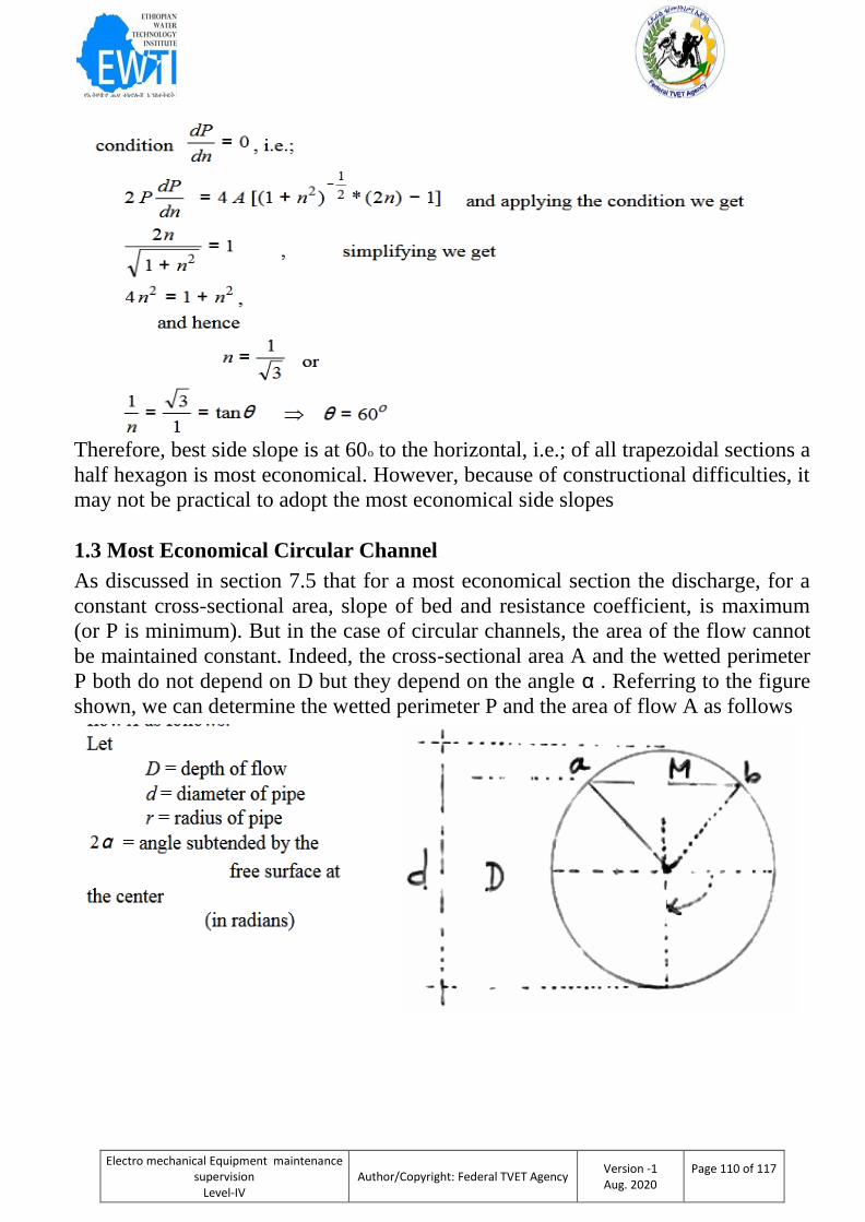
Electro mechanical Equipment maintenance supervision
Level-IV
Author/Copyright: Federal TVET Agency Version -1 Aug. 2020
Page 110 of 117
Therefore, best side slope is at 60o to the horizontal, i.e.; of all trapezoidal sections a
half hexagon is most economical. However, because of constructional difficulties, it
may not be practical to adopt the most economical side slopes
1.3 Most Economical Circular Channel
As discussed in section 7.5 that for a most economical section the discharge, for a
constant cross-sectional area, slope of bed and resistance coefficient, is maximum
(or P is minimum). But in the case of circular channels, the area of the flow cannot
be maintained constant. Indeed, the cross-sectional area A and the wetted perimeter
P both do not depend on D but they depend on the angle α . Referring to the figure
shown, we can determine the wetted perimeter P and the area of flow A as follows
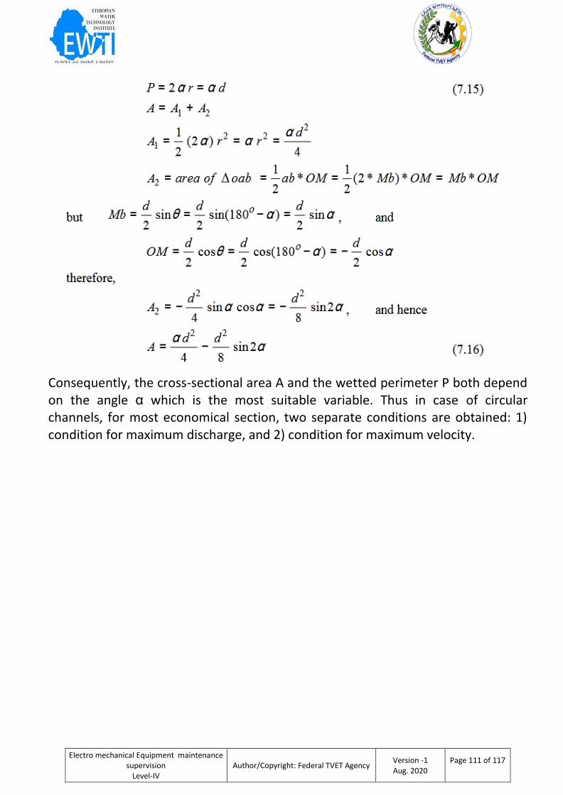
Electro mechanical Equipment maintenance supervision
Level-IV
Author/Copyright: Federal TVET Agency Version -1 Aug. 2020
Page 111 of 117
Consequently, the cross-sectional area A and the wetted perimeter P both depend on the angle α which is the most suitable variable. Thus in case of circular channels, for most economical section, two separate conditions are obtained: 1) condition for maximum discharge, and 2) condition for maximum velocity.
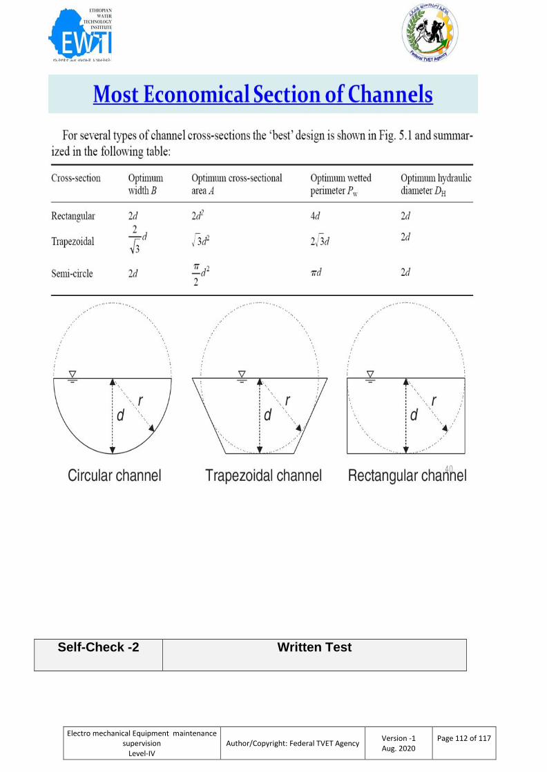
Electro mechanical Equipment maintenance supervision
Level-IV
Author/Copyright: Federal TVET Agency Version -1 Aug. 2020
Page 112 of 117
Self-Check -2 Written Test

Electro mechanical Equipment maintenance supervision
Level-IV
Author/Copyright: Federal TVET Agency Version -1 Aug. 2020
Page 113 of 117
Directions: Answer all the questions listed below. Use the Answer sheet provided in the next
page:
1. What are the most economical flow channels?
2. Describe each type of economic flow channel?
A. Horizontal
B. Trapezoid
C. Circular
Information sheet -2 Differentiate a partial flow chart is used to identify
the depth of flow for maximum discharge and
maximum velocity
Electro mechanical Equipment maintenance supervision
Level-IV
Author/Copyright: Federal TVET Agency Version -1 Aug. 2020
Page 114 of 117
5.2. Differentiate A partial flow chart used to identify the depth of flow for maximum discharge
and maximum velocity
The variation of flow velocity within a cross-section complicates the hydraulic analysis, so the engineer
... Note that the depth used should be the actual depth of flow, ..... exits over the top of the weir, and,
as with orifices, the point of maximum contraction is ... : V-Notch Weir Coefficients of Discharge — .C
= Discharge coefficient from... H = Depth off low above elevation of crest in feet
(approach velocity shall be ... Weirs are generally used as measuring and hydraulic control devices. ....
pipe 48 inches in diameter or smaller, and to a maximum of 6 inches for pipe. generally flow faster,
whereas rivers are deeper, wider and more ... friction against the bottom and banks causes
the velocity to decrease from a maximum ..... With the velocity obtained in terms of the
water depth and discharge [u = Q/A ..... to hold and can be used to determine the changes in
the flow across.
Flow Conveyance discharge Water travels downhill from points of higher energy to points of lower energy
(unless forced to do otherwise) until it reaches a point of equilibrium, such as an ocean. This tendency is
facilitated by the presence of natural conveyance channels such as brooks, streams, and rivers. The water’s
journey may also be aided by man-made structures such as drainage swales, pipes, culverts, and canals.
Hydraulic concepts can be applied equally to both man-made structures and natural features. Area, Wetted
Perimeter, and Hydraulic Radius The term area refers to the cross-sectional area of flow within a channel. When
a channel has a consistent cross-sectional shape, slope, and roughness, it is called a prismatic channel. If the flow
in a conveyance section is open to the atmosphere, such as in a culvert flowing partially full or in a river, it is said
to be open-channel flow or free-surface flow. If a channel is flowing completely full, as with a water distribution
pipe, it is said to be operating under full-flow conditions. Pressure flow is a special type of full flow in which
forces on the fluid cause it to push against the top of the channel as well as the bottom and sides. These forces
may result from, for example, the weight of a column of water in a backed-up sewer manhole or elevated
storage tank. A section’s wetted perimeter is defined as the portion of the channel in contact with the flowing
fluid.
Maximum Velocity;- the velocity of a section is not constant throughout the cross-sectional area. Instead, it
varies with location. The velocity is zero where the fluid is in contact with the conduit wall. So The variation of
flow velocity within a cross-section complicates the hydraulic analysis, so the engineer usually simplifies the
situation by looking at the average (mean) velocity of the section for analysis purposes. This average velocity is
defined as the total flow rate divided by the cross-sectional area, and is in units of length per time. V = Q/ A
where V = average velocity (m/s, ft/s) Q = flow rate (m3 /s, ft 3 /s) A = area (m2 ,ft 2 ) Steady Flow Speaking in
terms of flow, the word steady indicates that a constant flow rate is assumed throughout an analysis. In other
words, the flow velocity does not change with respect to time at a given location. For most hydraulic calculations,
this assumption is reasonable. A minimal increase in model accuracy does not warrant the time and effort that
would be required to perform an analysis with changing (unsteady) flows over time. When analyzing triver
networks, storm sewers, and other collection systems in which it is desirable to vary the flow rate at different
locations throughout the system, the network can often be broken into segments
Velocity partial flow discharge chart
There are some basic issues common to both the types are followingydraulics Prof. B.
1. Shape of the cross section of the canal.
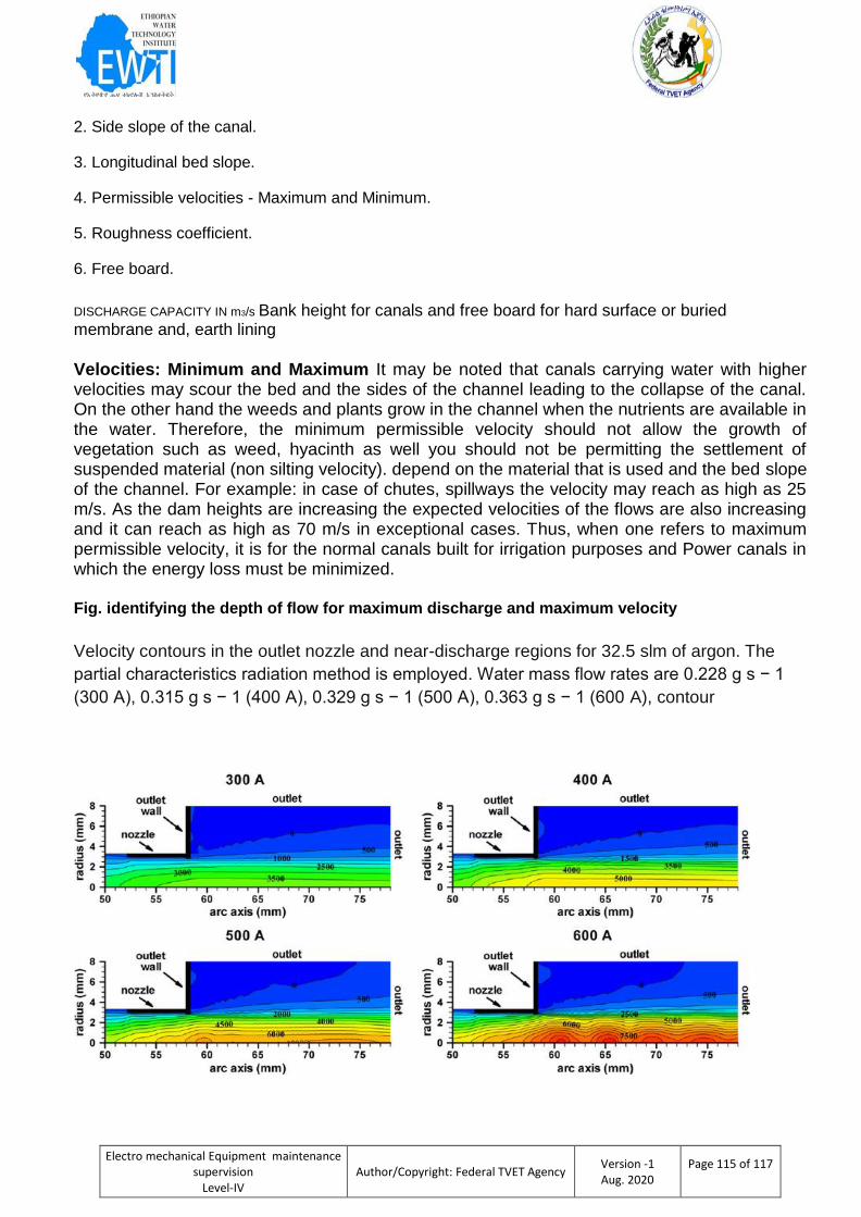
Electro mechanical Equipment maintenance supervision
Level-IV
Author/Copyright: Federal TVET Agency Version -1 Aug. 2020
Page 115 of 117
2. Side slope of the canal.
3. Longitudinal bed slope.
4. Permissible velocities - Maximum and Minimum.
5. Roughness coefficient.
6. Free board.
DISCHARGE CAPACITY IN m3/s Bank height for canals and free board for hard surface or buried membrane and, earth lining
Velocities: Minimum and Maximum It may be noted that canals carrying water with higher velocities may scour the bed and the sides of the channel leading to the collapse of the canal. On the other hand the weeds and plants grow in the channel when the nutrients are available in the water. Therefore, the minimum permissible velocity should not allow the growth of vegetation such as weed, hyacinth as well you should not be permitting the settlement of suspended material (non silting velocity). depend on the material that is used and the bed slope of the channel. For example: in case of chutes, spillways the velocity may reach as high as 25 m/s. As the dam heights are increasing the expected velocities of the flows are also increasing and it can reach as high as 70 m/s in exceptional cases. Thus, when one refers to maximum permissible velocity, it is for the normal canals built for irrigation purposes and Power canals in which the energy loss must be minimized.
Fig. identifying the depth of flow for maximum discharge and maximum velocity
Velocity contours in the outlet nozzle and near-discharge regions for 32.5 slm of argon. The
partial characteristics radiation method is employed. Water mass flow rates are 0.228 g s − 1
(300 A), 0.315 g s − 1 (400 A), 0.329 g s − 1 (500 A), 0.363 g s − 1 (600 A), contour
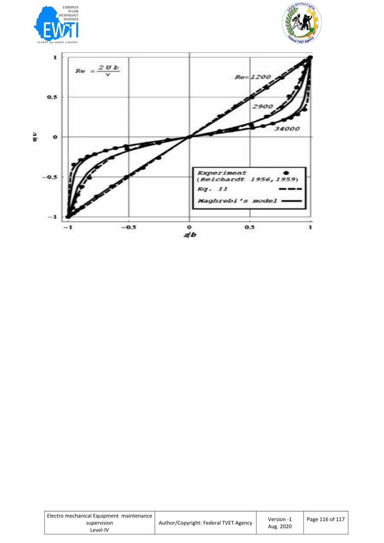
Electro mechanical Equipment maintenance supervision
Level-IV
Author/Copyright: Federal TVET Agency Version -1 Aug. 2020
Page 116 of 117

Electro mechanical Equipment maintenance supervision
Level-IV
Author/Copyright: Federal TVET Agency Version -1 Aug. 2020
Page 117 of 117
Self-Check -2 Written Test
Directions: Answer all the questions listed below. Use the Answer sheet provided in the next
page:
1;-Explain most economical channel?
2;-What is the hydraulic diameter?
3;-what are flow control valves?
4;-what is difference b/n trapezoidal and rectangular chanels?