Embed Size (px)
Citation preview

Thomas Sundqvist
Electricity Externality Studies: Do the Numbers Make Sense?
2000:14
LICENTIATE THESIS
Licentiate thesis
Institutionen för Industriell ekonomi och samhällsvetenskapAvdelningen för Nationalekonomi
2000:14 • ISSN: 1402-1757 • ISRN: LTU-LIC--00/14--SE

Electricity Externality Studies
Do the Numbers Make Sense?
THOMAS SUNDQVIST


I
ABSTRACT
During the 1980s and 1990s a number of studies have addressed the problem of
valuing the externalities arising from electricity production. The main objective of
these studies has been to guide decision-making with respect to future fuel choices.
However, the results of the studies have been ambiguous, especially when one looks
at the size of externality estimates. These sometimes differ with several orders of
magnitude, and in this sense previous studies provide poor guidance for policy
makers. Hence, the purpose of this thesis is twofold; first to critically survey existing
electricity externality studies (especially in the context of comparability and policy
relevance), and more specifically to investigate whether there are any systematical
explanations to the apparent discrepancy of externality estimates.
The thesis starts by reviewing the theoretical and practical approaches to the
valuation of externalities. After that, five representative and influential studies are
critically reviewed and compared, this both to illustrate how externalities may be
appraised and the problems arising when doing this. In particular it attempts to
highlight important differences among studies. The review shows that the
comparability of studies is generally limited because studies differ in scope and
hence that it is hard to draw reliable conclusions. Based on the review and
acknowledging that part, but not all, of the disparity in externality estimates may be
attributed to the specific location of the plant in question, the following main
hypotheses are formed and qualitatively examined; first the methodological
approach matters, i.e., the choice of method affects the size of externality estimates;
further that differences in thoroughness and basic assumptions among studies may
provide parts of the explanation.
The qualitative analysis points to the fact that the methodological choice may
affect estimates, that the thoroughness of approach in the studies affects the
magnitude of estimates, and also that the basic assumptions of the studies may
influence results considerably.
Quantitative analysis, relying on the statistical technique ANOTA (ANalysis
Of TAbles), is also attempted. The ANOTA-analysis indicates that the choice of

II
methodological approach matters. There also seems to be statistically significant
differences among fuels, i.e., that the renewables (e.g., solar and wind power) seem
to, on average, cause lower impacts than the fossil fuels. The analysis could however
not find any (statistical) support for the most common explanation to the disparity of
estimates, i.e., that the majority of the differences among studies are due to plant
location. Overall, it is concluded that, the comparison of electricity externality studies
is made harder by the fact that the scope and methodological approach differ among
studies, thus reducing the studies’ relevance to policy.
Keywords
Externalities, Electricity, Environmental Valuation, ANOTA, Damage Costs,
Abatement Costs, Revealed Preference, Welfare Theory, Government Policy

III
TABLE OF CONTENTS
ABSTRACT ............................................................................................................................... I
LIST OF FIGURES AND TABLES ....................................................................................... V
ABBREVIATIONS................................................................................................................VII
ACKNOWLEDGEMENTS................................................................................................... IX
Chapter 1 INTRODUCTION ................................................................................................. 1
1.1 Background .................................................................................................................... 1
1.2 Purpose ........................................................................................................................... 3
1.3 Scope ............................................................................................................................... 3
1.4 Methodological Issues .................................................................................................. 3
1.5 Outline ............................................................................................................................ 4
Chapter 2 VALUATION OF EXTERNALITIES IN THEORY AND PRACTICE........... 5
2.1 Introduction ................................................................................................................... 5
2.2 Theory of Externalities ................................................................................................. 5
2.3 Valuation in Theory ...................................................................................................... 8
2.3.1 Preference Revelation ............................................................................................ 9
2.3.2 Total Economic Value.......................................................................................... 12
2.4 Valuation in Practice................................................................................................... 12
2.4.1 Abatement Cost Approaches.............................................................................. 13
2.4.2 Damage Costing ................................................................................................... 15
2.4.3 Monetization ......................................................................................................... 17
2.5 Concluding Remarks .................................................................................................. 22
Chapter 3 VALUATION OF ELECTRICITY EXTERNALITIES: A CRITICAL SURVEY
OF EMPIRICAL STUDIES ................................................................................................... 25
3.1 Introduction ................................................................................................................. 25
3.2 Five Representative Externality Studies .................................................................. 27
3.2.1 Hohmeyer [1988] .................................................................................................. 28
3.2.2 Bernow and Marron [1990], and Bernow et al. [1991] .................................... 35
3.2.3 Carlsen et al. [1993] .............................................................................................. 40
3.2.4 European Commission [1995c & f] .................................................................... 44
IV
3.2.5 van Horen [1996] .................................................................................................. 59
3.3 Comparing the Studies............................................................................................... 65
3.4 Concluding Remarks .................................................................................................. 71
Chapter 4 EXAMINING THE DISPARITY OF EXTERNALITY ESTIMATES............. 73
4.1 Introduction ................................................................................................................. 73
4.2 Overview of Electricity Externality Studies ............................................................ 73
4.3 Why do the Externality Estimates Differ? ............................................................... 77
4.3.1 Site and Country Specificity ............................................................................... 79
4.3.2 Convergent Validity ............................................................................................ 80
4.3.3 Repetitive Validity ............................................................................................... 82
4.3.4 Thoroughness ....................................................................................................... 83
4.3.5 Assumptions ......................................................................................................... 84
4.4 Quantitative Analysis of Externality Studies .......................................................... 85
4.4.1 The Choice of Model............................................................................................ 86
4.4.2 The ANOTA Model ............................................................................................. 86
4.4.3 ANOTA Analysis of Externality Studies .......................................................... 88
4.5 Concluding Remarks .................................................................................................. 98
Chapter 5 A SUMMARY OF THE MAIN FINDINGS..................................................... 99
REFERENCES ...................................................................................................................... 103
Appendix 1 ELECTRICITY EXTERNALITY STUDIES ...................................................... i
Appendix 2 STUDIES INCLUDED IN THE ANOTA ANALYSIS ................................vii

V
LIST OF FIGURES AND TABLES
Figures
2.1: Marginal Abatement and Damage Costs ...................................................................14
2.2: The Top-Down Approach ............................................................................................16
2.3: The Impact Pathway (Bottom-Up Approach) ...........................................................17
2.4: Overview of Impact Valuation Techniques ...............................................................18
4.1: Range of External Cost Estimates for Different Fuel Sources .................................74
4.2: Methodologies Used in the Appraisal of Electricity Externalities Over Time......76
4.3: External Costs from Fossil Fuels Over Time .............................................................77
4.4: Range of External Costs for Fossil Fuels in Different Developed Countries ........80
4.5: Range of External Costs for Different Methodologies (Fossil Fuels) .....................81
4.6: Bottom-Up Damage Cost Estimates for Fossil Fuels Over Time............................83
Tables
1.1: Range of External Cost Estimates for Some Fuels ......................................................2
2.1: Relevance of Techniques to Value Specific Effects ...................................................23
3.1: Overview of Reviewed Externality Studies...............................................................26
3.2: Externalities Quantified and Monetized in the Hohmeyer Study..........................32
3.3: External Cost Development for Greenhouse Gases .................................................37
3.4: Externalities Quantified and Monetized in the Bernow et al. Study .....................39
3.5: Estimated External Costs in the Carlsen et al. Study ...............................................43
3.6: Assumed Air Pollutant Emission Levels in the ExternE Coal Study.....................45
3.7: Dose-Response Functions Employed by the ExternE Coal Study..........................46
3.8: Global Warming Damage Estimates for the Coal Fuel Cycle .................................53
3.9: Externalities Quantified and Monetized in the ExternE Coal Study .....................54
3.10: Externalities Quantified and Monetized in the ExternE Hydro Study..................58
3.11: Externalities Quantified and Monetized in the van Horen Study..........................64
4.1: Descriptive Statistics of Externality Studies ..............................................................75
4.2: Value of Air Emission Reductions in California .......................................................82
4.3: Assumed Emission Levels of SOx, NOx and CO2 for Coal .......................................85

VI
4.4: Statistical Overview of Studies Included in the ANOTA Analysis........................88
4.5: Total Projected Generation Costs for New Capacity................................................89
4.6: Model Specification .......................................................................................................94
4.7: Results of the ANOTA Analysis of Externality Studies...........................................95
4.8: 95-Percent Confidence Intervals for the Estimated Equations ...............................98

VII
ABBREVIATIONS
ANOTA ANalysis Of TAbles
BACT Best Available Control Technology
BPA Bonneville Power Administration
Btu British thermal unit
CA California
CEC California Energy Commission
CFC Chlorofluorocarbon
CH4 Methane
CO Carbon Monoxide
CO2 Carbon Dioxide
CV Compensating Variation
CVM Contingent Valuation Method
DOE Department of Energy
E Emissions
EC European Commission
EEC Expected External Cost
EF Emission Factor
EIA Energy Information Administration
EPA Environmental Protection Agency
EU European Union
EV Equivalent Variation
ExternE Externalities of Energy
FGD Flue Gas Desulfurization
GDP Gross Domestic Product
GWP Global Warming Potential
GWh Gigawatt hour
HR Heat Rate
IEA International Energy Agency
IPCC Intergovernmental Panel on Climatic
Change
kWh Kilowatt hour
LCA Life-Cycle Analysis
MAC Marginal Abatement Cost
MDC Marginal Damage Cost
MW Megawatt
NAAQS National Ambient Air Quality
Standards
NEA Nuclear Energy Agency
NOx Oxides of Nitrogen
N2O Nitrous Oxide
O3 Ozone
OLS Ordinary Least Squares
ORNL Oak Ridge National Laboratory
OTA Office of Technology Assessment
PM Particulate Matter
PPP Purchasing Power Parity
PV Photovoltaic
RfF Resources for the Future
ROG Reactive Organic Gases
SCR Selective Catalytic Reduction
SO2 Sulfur Dioxide
SOx Oxides of Sulfur
TM Trace Metals
TSP Total Suspended Particles
TWh Terawatt hour
UK United Kingdom
US United States
USD US Dollar
VED Value of Environmental Damage
VOC Volatile Organic Compounds
VSL Value of a Statistical Life
WTA Willingness To Accept compensation
WTP Willingness To Pay


IX
ACKNOWLEDGEMENTS
First of all I wish to express my gratitude to Professor Marian Radetzki, Division of
Economics at Luleå University of Technology, for providing me with the opportunity
to pursue a licentiate degree, for his constant encouragements and for valuable
comments on various drafts of the present thesis. Thank you Marian!
The second person that I want to mention is my seemingly inexhaustible
supervisor Dr. Patrik Söderholm. He has repeatedly read and commented on my
work, even when there was almost nothing to comment on. His importance for the
completion of this thesis cannot be emphasized enough. Thank you Patrik!
Furthermore, the generous financial support from Vattenfall AB is gratefully
acknowledged.
Past and present members of the Advisory Board, who together supervise
the research at the Division, have all in one way or another provided invaluable help
that has contributed to the successful completion of this thesis. They are: Professor
Ernst Berndt, MIT; Professor James Griffin, Texas A&M University; Professor
Thorvaldur Gylfason, University of Iceland; Dr. David Humphreys, Rio Tinto Ltd.
London; Dr. Keith Palmer, N M Rothschild & Sons Ltd. London; and Professor John
Tilton, Colorado School of Mines. Thank you All! I especially want to express my
gratitude to Professor Tilton, for making it possible for me to spend one semester at
the Colorado School of Mines during the fall 1997, and to Professor Griffin, for
making it possible for me to attend Texas A&M next fall.
I am also grateful to my other colleagues and friends at the Division;
Anderson, Anna, Bo, Christer, Jerry, Kristina, Mats, Olle, Robert, Staffan, and Stefan
have all provided valuable comments or have in other ways helped in the completion
of this thesis. I would especially like to thank Jerry for taking it upon himself to act as
a discussant at the pie-seminar. Also, in our complex world, the writing of a thesis
would not be possible without constant administrative help and guidance; thank you
Gerd and Gudrun.

X
Thanks also go to Nils-Gustav Lundgren, Professor of Economic History. He
provided me with the statistical tools utilized in this thesis and clarified the meaning
of the results.
The thesis has further benefited from comments from the participants at a
lunch-seminar held at the Center for Business and Policy Studies (SNS) in Stockholm,
October 1999.
Finally, I wish to thank my family and friends for being there even if I have
not been very accessible lately.
Since I have received so much guidance along the way, I believe it is safe to
say that all remaining errors are mine.
Luleå, April 2000
Thomas Sundqvist

1
Chapter 1
INTRODUCTION
1.1 Background
In recent years, increasing attention from policy makers and researchers has been
given to the external costs and benefits of energy production. Several major studies
have addressed the issue. Examples include the ExternE-project in the European
Community [EC, 1995a-f] and, in the US, the New York State Environmental
Externality Cost Study [Rowe et al., 1995].1 The general aim of these studies has been
to guide policy-making, i.e., to provide a solid basis for new regulations and taxes,
and to aid decision-makers in their choice of fuels with which to expand future
energy producing capacity. According to economic theory utilities and regulators
should base their choices of energy sources on the full costs and benefits of using a
resource, i.e., on the private as well as on the external costs and benefits of resource
use. However, external costs and benefits are not always easy to assess. In most
cases, the affected goods are not traded in a market and their values are thus not
directly identifiable. Economists normally rely on individuals’ willingness to pay or
accept to elicit values for unpriced goods; these measures are intended to reflect
individual preferences for or against change (i.e., as caused by the impact from an
externality). Economic theory, hence, directs us how to go about assessing
externalities and provides us with the methods necessary to make this assessment.
However, the actual assessments that have been carried out have provided a
far from clear-cut picture. For the studies that have been completed the externality
estimates produced for each electricity source range from very high effects to almost
insignificant effects. Table 1.1 illustrates this phenomenon.
1 For an overview of a majority of the electricity externality studies carried out during the last two
decades, see Appendix 1.

2
Table 1.1: Range of External Cost Estimates for Fossil Fuels (US cents/kWh 1998)
Coal Oil Gas
Low 0.004 0.05 0.01
High 2000.00 680.00 317.00
Mean 88.58 45.74 15.26
Median 6.53 9.11 3.38
N= 35 18 28
Sources: Appendix 1.
Table 1.1 is based upon the externality cost estimates for fossil fuels (e.g.,
coal, oil and gas) from a number of externality-costing studies carried out during the
1980s and 1990s. Looking at the table it is easily discernable that the different studies
have produced externality estimates that differ considerably (i.e., several thousand
times). Furthermore, the ranges intertwine, i.e., none of the fuels can clearly be said
to impose lower external costs on society than the others (see also section 4.1). Thus,
the results are ambiguous and may therefore be a poor guide for policy. In order to
be useful for policy-making, the different studies must produce estimates that can be
compared and used in rational decision-making. Based on previous research efforts
this appears not to be the case. Hence, some effort aimed at addressing the
comparability of studies, in particular in the policy context, is motivated. One way of
approaching this issue is to critically survey the existing research on electricity
externalities, and highlight important theoretical and empirical differences between
them.
What is more, the reasons to the apparent disparity are unclear. Several
suggestions have been raised in the literature, but these are also somewhat
ambiguous. Some researchers have suggested that the different methodologies
available tend to produce different results (e.g., Joskow [1992]); while other stress the
importance of site specificity (e.g., Lee [1997]), i.e., that damages are due to the
specific location of the plant; or that differences in scope and comprehensiveness
among studies may be one important explanation (e.g., Stirling [1998]), etc. A
clarification of which of these is the most important is useful. For example, if site-
specificity can be established to be a valid explanation to the disparities, then no

3
general externality estimates may be developed, i.e., no direct comparability between
different sites. Evidently, more work is needed to identify the reasons to the disparity
of externality estimates and thus to whether the results of existing studies provide a
basis on which rational decisions may be made.
1.2 Purpose
The purposes of this thesis are:
• to provide a critical survey of existing electricity externality studies, especially
in the context of comparability and policy relevance.
• to analyze if there are any systematical explanations to the discrepancy in
externality estimates of earlier studies.
1.3 Scope
The study deals solely with the externalities arising from electricity production; other
sources of energy are thus not considered in this study. Furthermore, no own
assessments of externalities will be done. The focus will be exclusively on the results
presented in earlier studies carried out during the 1980s and 1990s.
1.4 Methodological Issues
The analysis in this thesis is done in two steps. The first part of the analysis carried
out comprises a deep survey of five earlier studies (chapter 3). This first part of the
thesis relies on qualitative analysis with a basis in economic theory. The qualitative
analysis is aimed at addressing both purposes, i.e., to assess the relevance of previous
research for policy as well as to find explanations to the discrepancies of externality
estimates. As this part of the analysis attempts to scrutinize every detail in a sample
of earlier studies, it forms the basis for the analysis in the second part of the thesis.
The second part of the analysis consists of a broader analysis specifically
aimed at explaining the differences in estimates (chapter 4). First, hypotheses, are,
formed based on the analysis carried out in chapter 3. These are then qualitatively
scrutinized. In the second part of chapter 4, quantitative analysis, specifically aimed
at finding systematical explanations to the disparities of externality estimates, is
employed. The method used, ANOTA (ANalysis Of TAbles), is a statistical technique
to explore relationships between categorical (i.e., discrete) variables. The method is,

4
hence, advantageous in comparison with, for example, OLS since it allows for
categorization of both the dependent variable and the independent variables.
ANOTA is applied to test the hypotheses that were developed and scrutinized in the
preceding qualitative analysis.
1.5 Outline
Chapter 2 starts by defining the concept of externalities and why externalities are a
problem. After that, theoretical and practical approaches to the assessment of
externalities are outlined.
In chapter 3, a deep and thorough review of five representative externality
studies is carried out. These studies are critically reviewed and discussed using
economic theory as a basis, this to illustrate how externalities may be assessed and
the methodological as well as practical problems (and possibilities) of this appraisal.
The identified issues are utilized as a starting point for the analysis carried out in
chapter 4.
Chapter 4 addresses the specific question of why the externality estimates
produced by the different studies differ considerably. The analysis in the chapter
focuses on all available studies and is divided into two parts; first, the different
studies are graphically and verbally discussed in line with hypotheses formulated
based on the review carried out in chapter 3. The second part of the analysis relies on
ANOTA analysis. Here the hypotheses posed are tested statistically.
Finally, in chapter 5, the main conclusions of the thesis are summarized and
the implications for policy are discussed.

5
Chapter 2
VALUATION OF EXTERNALITIES IN THEORY AND PRACTICE
2.1 Introduction
This chapter focuses on the theoretical and practical approaches to the valuation of
externalities, with an emphasis on the externalities arising from electricity
production. No attempt is made in the chapter to review theories and methods in any
detail, this since the focus in the present thesis primarily is on empirical results.
Consequently, the chapter serves mainly as a brief introduction and background. The
economic concept of value stems from individual preferences and is hence based on
utility theory. The theoretical foundations for ‘preference revelation’ in forms of
willingness to pay/accept are introduced in section 2.3. The practical approaches
(i.e., abatement and damage costing) to elicit willingness to pay/accept (i.e.,
monetize externalities) are then outlined in section 2.4. The chapter ends with some
concluding remarks in section 2.5. However, before we go on to discuss valuation
issues in theory and practice, we need to introduce and define the concept of
externalities (section 2.2).
2.2 Theory of Externalities
Economists have given the concept of externalities great attention ever since the days
of Alfred Marshall and his disciple Arthur C. Pigou in particular. However, the exact
definition and interpretation of the concept appears to be somewhat confused (e.g.,
Verhoef [1997]). 2
2 External costs and benefits have been given many different names in the literature. They are also
known as externalities, external effects, external diseconomies/economies, neighborhood effects, third
party effects, and adders (i.e., additional to the costs of production). The concept, however, remains
the same whatever name they are given.

6
There are many equivalent ways of defining an externality but one
comprehensive definition is [Perman et al., 1999, p. 129]:
"An external effect […] is said to occur when the production or consumption
decisions of one agent affect the utility of another agent in an unintended way,
and when no compensation is made by the producer of the external effect to the
affected party."
This definition, which follows the one derived by Baumol and Oates [1988],
thus states that an externality is an unpriced benefit or cost directly bestowed or
imposed upon one agent by the unintentional actions of another agent. Note that the
definition, as suggested by Mishan [1969], rules out any deliberate actions. The
argument, as raised by Mishan, for not considering the intentional action of an agent
to comprise an externality is that such an action may be handled within the existing
justice system, e.g., society will by itself internalize any deliberate effects.
Furthermore, the non-compensatory requirement is necessary for the externality to
cause inefficiencies and misallocations [Baumol & Oates, 1988]. Moreover,
externalities can occur in both the consumption and the production of a good and the
agent that unintentionally receives the external effect can in turn be either a
consumer or a producer.
Externalities cause market failures because they lead to an allocation of
resources that is non-optimal from society’s point of view. An externality hence
causes a type of situation in which the First Theorem of Welfare Economics fails to
apply, i.e., markets fail to accomplish Pareto efficiency.3 In this case market
intervention in order to achieve welfare improvements might be desirable.4 For
example, consider firm j that operates in a competitive market.5 Furthermore, assume
3 For more on this issue, see for example Varian [1992, Chapter 17] and Verhoef [1997]. 4 This market failure predicament excludes so-called pecuniary externalities that only have
distributional effects. What is under study here are technological externalities, i.e., externalities that
directly affect economic efficiency. This issue is more thoroughly discussed by Lesser et al. [1997, p.
111]. 5 The formal representation is based on Varian [1992, Chapter 24].

7
that firm j produces an output y that it sells at the market price p. Then the following
profit maximization problem can be formulated for firm j:
( )ycpymaxy
j −=π (2.1)
where c(y) is the (private) costs and j is the profit of producing y units of output for
firm j. The equilibrium amount of output, y*, is given by the first-order condition:
( )∗′= ycp (2.2)
showing that firm j should produce up to the point where prices equal marginal
(private) costs. However, suppose that the productive activity of firm j gives rise to
an external cost e(y), e.g., that the production of y units of output also yields y units
of pollution. The output y* is then too large from society’s point of view. Thus, in its
optimization firm j only accounts for its private (i.e., internal) costs and not for the
external costs that it imposes on society. In order to determine the efficient level of
production the firm should internalize the externality, thus incorporate the external
costs into its profit maximization problem, so that:
( ) ( )yeycpymaxy
j −−=π (2.3)
with the corresponding first-order condition:
( ) ( )ee yeycp ′+′= . (2.4)
The output ye is Pareto efficient; price is set to equal the sum of marginal private cost
and marginal external cost, i.e., the marginal social cost. Generally, the private costs
of a producer measure the best alternative uses of resources available, as reflected by
the market price of the specific resources used by a producer. The social costs of
production measure the best alternative use of resources available to society as a

8
whole. The sum of private and external costs constitutes the full social costs of
production [Pearce, 1995].
However, as Ayres and Kneese [1969] demonstrate in their seminal work,
unregulated markets will not themselves internalize externalities. In order for the
outcome in a market on which externalities are present to be efficient some kind of
government intervention is called for. One classic way of correcting the inefficiency
of an externality is through the use of a Pigovian tax (as originally suggested by
Pigou [1924]), i.e., setting a tax t on firm j’s production can effectively internalize the
external costs. The firm’s first-order condition for profit maximization then becomes:
( ) tycp +′= . (2.5)
If the corrective tax t is set to equal e’(ye) the firm will choose to produce the optimal
level of output ye as given by equation (2.4) and the external costs will be
internalized. However, this solution to the externality problem requires that the tax
setting authority is able to identify the external cost function, i.e., e(y).6 How do we go
about assessing the size of e’(ye)? The theoretical bases to such valuation are
discussed in section 2.3 while the practical approaches are discussed in section 2.4.
2.3 Valuation in Theory
Externalities have direct and real effects on consumers’ utility and thus on value.
Externalities are, however, generally not reflected in market transactions and
consequently not in prices. In order to approach the socially optimal level of any
production activity (e.g., as derived in equation 2.4) it is necessary to evaluate the
impacts associated with any externalities the activity produces. This is accomplished
by ‘monetizing’ individuals’ preferences.
6 Other solutions to the externality problem have been suggested. See for example Coase [1960] who
proposes that markets alone, given that bargaining between affected agents is accomplished, can
achieve an efficient solution.

9
2.3.1 Preference Revelation
The economic value of a resource or service is based on individual preferences;
economic valuation is, consequently, about ‘measuring peoples preferences.’ The
valuation process is anthropocentric and the resulting valuations are in monetary
terms because of the way that preference revelation is sought. That is, by
investigating how much people are willing to pay (WTP) for or against change, or
how much they are willing to accept in compensation (WTA) for allowing the
change, economist obtain direct welfare measures associated with specific effects.
The resulting monetary estimates are advantageous because they allow for
comparison between ‘traded’ and ‘non-traded’ goods and services.7 Using individual
preferences as a basis for economic value excludes any intrinsic values from the
analysis. This does not mean that these types of values do not exist nor that they are
irrelevant. Intrinsic values can simply not be handled within an economic
framework. This indicates that economic value is not a comprehensive measure of
‘total value’ something that has to be considered by decision-makers [Pearce, 1993].
As a result, what is being valued is not the externality impact in itself, but rather
individuals’ preferences for or against change.8 For example, consider the welfare of
individual i and assume that individual i’s utility (Ui) depends on a vector of private
consumption possibilities (q) and an environmental quality index (z).9 Hence,
individual i’s utility function:
( )zUU ii ,q= , (2.6)
shows the various combinations of q and z from which the individual derives utility.
Further, assume that for any given level of z the individual is better off if q increases.
Now consider a project that causes the environmental quality to change from z0 till z1
7 Expressing values in monetary terms is not necessarily the only way of assessing economic value;
other means of addressing this issue may be at least as relevant. It is, however, normally the most
convenient unit for economic analysis. 8 For more discussion on this issue, see Perman et al. [1999, Chapter 14]. 9 For a more advanced treatment, see Johansson [1993] and Freeman [1993].

10
(e.g., due to an impact from an externality) and assume that this change does not
affect q (i.e., that the individual’s income remains constant). The project thus causes
individual i’s utility or welfare to change by:
( ) ( )0010 z,Uz,U ii qq − . (2.7)
If this change is positive (e.g., an environmental improvement due to an external
benefit) individual i is better off, his/her utility has increased, and contrary if the
change is negative (e.g., an environmental deterioration due to an external cost)
individual i is worse off. However, since utility is not directly observable we need to
find ways of assessing this welfare change. Two measures of welfare changes are the
compensating and equivalent variations.
First, consider the compensating variation (CV) measure, this is the amount
associated with the move from z0 till z1 at the initial level of consumption (q0) such
that:
( ) ( )1000 z,CVUz,U ii −= qq . (2.8)
CV is the maximum amount of money that can be taken from the individual while
leaving him/her just as well of as before an improvement in environmental quality.
Hence, CV is the willingness to pay for an improvement in environmental quality. If
environmental quality deteriorates, CV is the minimum amount of money that must
be given to the individual in order to compensate him/her for the loss in
environmental quality. Thus in the case of a welfare deterioration, CV measures
willingness to accept compensation [Johansson, 1993].
The second monetary measure, equivalent variation (EV), is the amount
associated with the move from z1 to z0 at q0, which corresponds to:
( ) ( )0010 z,EVUz,U ii += qq . (2.9)

11
EV is the minimum amount of money that must be given to the individual to make
him/her just as well of as he/she could have been after an improvement in
environmental quality (i.e., WTA). Similarly, if environmental quality deteriorates
EV is the maximum amount the individual is willing to pay to prevent that
deterioration (i.e., WTP) [Ibid.].
Hence, all externalities should, according to utility theory, be valued by
seeking one of the following measures of individuals’ valuations:
a) the WTP to avoid an external cost (EV for a welfare deterioration),
b) the WTP to reduce an external cost (CV for a welfare improvement),
c) the WTA compensation for damage done from an external cost (CV for a
welfare deterioration), or
d) the WTA to forgo an external benefit (EV for a welfare improvement).
The presumption is that the WTP/WTA concepts will not deviate that much. Willig
[1976] shows that this actually should be the case, provided that income and wealth
effects are sufficiently small.10 More specifically Willig argues that the CV and EV
measures of welfare change should converge when considering an exogenous price
change. He shows that under specific assumptions regarding the assignment of
property rights and the source of the exogenous price change in question, WTP and
WTA correspond to CV and EV, respectively, and thus that WTP and WTP should
also converge.11 However, it turns out that in empirical studies WTA measures tend
to be substantially higher than WTP measures for the same change.12 Hanemann
[1991] considers a case when quantity is exogenously changed, and concludes that a
disparity between WTP and WTA is theoretically credible. Hence, while Willig’s
results are theoretically valid when the change is caused by prices they may not be
10 Willig demonstrates that the theoretical divergence between the measures should not be more than
10 percent. 11 Willig also show that, even though it is not a correct welfare measure, consumer surplus may be
used to approximate CV or EV. 12 The disparities between the two measures have been identified using questionnaire techniques such
as contingent valuation. Kahneman et al. [1990] have for example looked at several survey studies that
have used both WTP and WTA. They found that the mean WTA measures exceeded mean WTP
measures by factors ranging from 2.6 to 16.5.

12
when the source of the change is quantity. Thus, the choice of WTP or WTA as a
measure of value when considering an externality may affect the size of the resulting
externality estimate.
2.3.2 Total Economic Value
The economic value of a resource or service comprises use as well as non-use values.
The use values include direct use values, i.e., the utility gained from consumption,
indirect use values, i.e., the utility gained vicariously from the consumption of others,
option values, i.e., the utility gained from possible use in the future, and quasi-option
values, i.e., the utility gained through preserving options for future use [Pearce &
Turner, 1990; and Perman et al., 1999]. Non-use values comprise existence values, i.e.
values related to the existence of a resource as such, unrelated to any present or
future use of the resource. The total economic value of a resource (i.e., the sum of the
use and non-use values) can be utilized as a measure of all the types of values that
derives from human preferences, and that, hence, are amendable to economic
analysis [Perman et al., 1999]. However, some values are harder to assess than others
and some valuation methods can only measure certain types of values (see also
section 2.4.3).
2.4 Valuation in Practice
In practice, total external costs (TEC) to society (expressed in monetary terms) from a
power generating activity can typically be characterized by the following equation
[Koomey & Krause, 1997]:
VEDSITEC ×= (2.10)
where SI is the Size of Insult (i.e., the quantified impact), in physical units and VED is
the Value of Environmental Damage, expressed in monetary terms per physical unit
of output. For example, for air pollutant impacts, that vary with fuel consumption,
and normalizing for common currency (e.g., US cents) and unit of service (e.g.,
delivered kWh) for ease of comparison, equation (2.10) may be rewritten as follows
[Ibid.]:

13
( ) ( ) ( ) ( )poundcentsVEDkWhBtuHRBtupoundsEFkWhcentsTEC ××= (2.11)
where EF is the Emission Factor, in pound per Btu of fuel consumed, and HR is the
Heat Rate of the power plant, in Btu per kWh.13 In equation (2.11) the emission factor
relates the physical impact to the physical amount of fuel combusted. The heat rate
converts the quantified impact into a physical amount per kWh. The amount is then
converted into monetary terms by the VED-parameter. Of the parameters in equation
(2.11), the first two (EF and HR) can be measured physically, while the VED-
parameter must be calculated relying on one (or a combination) of the following two
basic approaches:14
• the abatement cost approach, and
• the damage cost approach.
The abatement cost approach is based on the costs as implicitly revealed by policy
makers in their decisions (e.g., through regulations), while the damage cost approach
is based on the valuation of actual damage done. These approaches are discussed
below in sections 2.4.1 and 2.4.2 in turn. These overall approaches rely, to a lesser
and greater extent, on specific monetary valuation methods. The most important
ones are outlined in section 2.4.3.
2.4.1 Abatement Cost Approaches
Abatement costs have been used extensively to approximate damage [Pearce et al.,
1992]. The abatement cost approach uses the costs of controlling or mitigating
damage from, for example, emissions as an implicit value for the damage avoided
(i.e., regulatory revealed preference or ‘shadow pricing’). It, hence, analyzes existing
and proposed regulations in order to estimate the value that society implicitly places
on specific impacts. The analysis is aimed at identifying the marginal cost reduction
strategy as required in the legislation, which can then be taken as an estimate of the
value that the regulators (and thus society) have placed on the specific impact. That
13 Btu (British thermal unit) measures “the amount of heat necessary to raise one pound of water one
degree Fahrenheit” [Peirce, 1996, p. 10]. 14 Other possible approaches do exist. Examples include life cycle analysis (LCA) and polling systems,
but these are not generally considered as approaches to the assessment of externalities specifically.

14
is, a value that represents the regulator’s (and society’s) perception of the damage
associated with the impact in question [Bernow & Marron, 1990]. The approach
consequently gives a direct estimate of the external cost or benefit in question.
One of the serious caveats with the approach is that it relies on the rather
strong assumption that decision makers make optimal decisions, i.e., that they know
the true abatement and damage costs (or at the least base their decisions on some
reasonably accurate conception of these) [Pearce et al., 1992].
Figure 2.1 shows the marginal abatement costs (MAC) and marginal damage
costs (MDC) from some emissions (E). Given that the curve MDC shows the true cost
of the damage done by the emissions, and if decision makers choose to abate at level
E3 the abatement cost will underestimate the true damage cost and at level E1 the
abatement cost will overestimate the true damage. Only at abatement level E2
marginal abatement costs correctly measure marginal damage costs. Consequently,
unless the level of control or mitigation is socially optimal (i.e. at E2), the use of
abatement cost as a measure of damage provides a biased estimate of the true
external costs. Thus, the possibility that regulators have set the wrong standards in
terms of efficiency (e.g., E1 or E3) makes the use of abatement costs as a proxy for
marginal damage quite risky. The externality estimates resulting from the abatement
cost approach, hence, contain the potential for significant errors.
Figure 2.1: Marginal Abatement and Damage Costs
Emissions
Costs
MAC
MDC MDC´
E1 E3 E2

15
Moreover, as Joskow [1992] notes, abatement cost will only be representative
of damage cost when it is derived from the pollution control strategy that gives the
least cost of control, i.e., at the minimum cost solution. According to Joskow the least
cost solution can only be achieved when the following conditions are met:
• All polluting sources in a region must be subject to uniform emission
regulations.
• Each source must abate pollution at the lowest possible cost.
• For any given level of pollution, the marginal cost of control must be equated
across all sources.
If one or more of these conditions are violated then the observed cost of control will
tend to overestimate true damage costs.
Another limitation affecting the abatement approach is that society’s
preferences change over time as information, analysis, values and policies change
[Bernow & Marron, 1990]. A clear limitation with the abatement cost approach is
then that past revealed preferences may bear little relation to actual impacts today
and their current value to society. Any valuation of externalities must consequently
rely on the implicit value that society currently places on the damage associated with
the impacts from these effects. Hence, this built-in ‘tautology’ of the approach, as
Joskow [1992] also notes, means that estimates need to be constantly revised as
regulations change.
2.4.2 Damage Costing
The damage cost approach is aimed at empirically measuring the net economic
damage arising from an externality, i.e., the actual costs and benefits of externalities
[Clarke, 1996]. It can be subdivided into two main categories:
• Top-Down, and
• Bottom-Up.
Top-Down
Top-down approaches make use of highly aggregated data to estimate costs of
particular pollutants. Top-down studies are typically carried out at national or
regional level, using estimates of total quantities of pollutants and estimates of total

16
damage caused by the pollutants [EC, 1995a]. More specifically, as illustrated in
figure 2.2, some estimate of national damage is divided by total pollutant depositions
to obtain a measure of damage per unit of pollutant [Pearce, 1995].
National damageestimate
% of damageattributable to activity
National estimate ofpollutant from activity
Estimated damage/unit ofpollutant from activity
Figure 2.2: The Top-Down Approach
Source: Adapted from EC [1995a].
The main critique against the top-down approach is that it ‘generically’
cannot take into account the site specificity of many types of impacts, nor the
different stages of the fuel cycle. Another argument that has been raised against the
approach is that it is derivative, this since it depends mostly on previous estimates
and approximations [Clarke, 1996].
Bottom-Up
In the bottom-up approach damages from a single source are typically traced,
quantified and monetized through damage functions/impact pathways (figure 2.3
outlines the approach). It makes use of technology-specific data, combined with
dispersion models, information on receptors, and dose-response functions to
calculate the impacts of specific externalities [Clarke, 1996].
The bottom-up approach has been criticized for that it tends to include only a
subset of impacts, focusing on areas where data is readily available and where, thus,
impact pathways can easily be established. Consequently bottom-up studies tend to
leave out potentially important impacts where data is not readily available [Ibid.].
Bernow et al. [1993] caution that the bottom-up approach is reliant on models that
may not adequately account for complexities in ‘the real world’, especially noting

17
that there may be synergistic effects between pollutants and environmental stresses,
and that there may be problems in establishing the timing of effects (i.e., between
exposure and impact). The argument is hence that bottom-up approaches may not be
sufficiently transparent. Still, this is the approach that is the most ‘direct’ and most in
line with economic theory. As is evident by the methodological choice in recent
externality studies it is also the most preferred approach to the assessment of
externalities in the electricity sector (see also chapter 4).
Emissions & otherimpacts
Changed Concentrationsand Other Conditions, by
Location
Transportmodel
Physical Impacts
Dose-Response Functions
EconomicValuationFunctions
Damages &Benefits
InternalizedDamages &
Benefits
ExternalDamages &
Benefits
é Technologyé Fuelé Abatement
technologyé Location
Fuel Cycle
AmbientConditions
Stock of Assets;Individuals
1. Name activities and estimate their emissions and other impacts
2. Model dispersion and change in concentrations of pollutants
3. Physically quantify emissions and other impacts
4. Translate physical quantities into economic damages and benefits
5. Distinguish externalities from internalized damages and benefits
Figure 2.3: The Impact Pathway (Bottom-Up Approach)
Source: Adapted from ORNL & RfF [1994a].
2.4.3 Monetization
There are several ways of tackling the problem of monetizing externalities. The first
two approaches discussed above (i.e., revealed preference and top-down damage
cost) directly give a monetary estimate of the damage associated with the impact
from an externality. The third possible approach, i.e., bottom-up damage cost,

18
however, in order to express damages in terms of WTP/WTA needs to translate the
identified and quantified impacts into monetary terms. Generally it can be said that
whenever market prices can be used as a basis for valuation, they should be used.
However, since externalities ‘by definition’ are external to markets, most impacts
from externalities are not reflected in markets (and thus in prices). Consequently any
attempt to monetize an externality when making use of the bottom-up damage cost
approach need to rely on impact valuation methods to estimate WTP/WTA. These
methods can be divided into:
• Direct methods, and
• Indirect methods
These will be briefly introduced below.15 An overview of the different methods is
given in figure 2.4. As can be seen in the figure, apart from direct and indirect
methods, there are also other alternatives to the monetization of externalities (i.e.,
benefit transfers, dose-response functions, and opportunity costs). These are also
introduced and briefly discussed below.
EXTERNALITY
Monetization of impact
Observable market No observable market
Market prices Indirect methods Direct methods Other methods
WTP/WTA
Productivity changes Income
changes Avertive expenditure Replacement
cost Travel cost Hedonic
pricing Trade-off game Contingent
valuation Stated preference
Experimental markets Hypothetical
markets
Dose- response Opportunity
cost Benefit transfer
Related markets
Figure 2.4: Overview of Impact Valuation Techniques
15 For a more advanced treatment, see for example Freeman [1993], Johansson [1993], and Smith [1997].

19
Direct Methods
Even if no information is available from existing markets, it may be possible to derive
values using direct methods that simulate markets. These methods are direct in the
sense that they are based on direct questions about, or are designed to directly elicit,
WTP/WTA. The direct methods can assess total economic values, i.e., use values as
well as non-use values (such as existence values). They can be sub-divided into
methods relying on experimental markets and methods relying on hypothetical
markets.
When experimental markets are used respondents actually carry out market
transactions (i.e., buy or sell goods) in an artificial market set up by researchers for
the goods in question. One example of such methods is trade-off games. In the trade-
off game respondents are offered two alternatives and are asked to choose between
them.16 The alternatives are defined in terms of their outcomes, they differ in the level
of one or more of the outcomes and one of the outcomes will be monetary. The
monetary outcome of the chosen alternative is then a measure of WTP/WTA.
Methods making use of hypothetical markets typically rely on questionnaires
or surveys to elicit WTP/WTA. Two examples of hypothetical methods are the
contingent valuation and the stated preference methods. The contingent valuation
method (CVM) is aimed at eliciting values using questions such as ‘what are you
willing to pay for X or to prevent Y’ and/or ‘what are you willing to accept to give
up B or allow A?’17 The technique, hence, makes use of direct questions to elicit
preferences by questionnaires. The resulting survey results need statistical treatment
to derive mean WTP values. The stated preference method is based on questionnaires
designed to elicit ranking of preferences.18 The respondents are asked to rank
alternatives in order of preference. The alternatives include the external effect to be
valued, substitutes for the effect and an alternative with known value (threshold
16 For an application of the trade-off game technique, see Adamowicz et al. [1998]. 17 An excellent presentation of CVM is given by Mitchell and Carson [1989]. See also Arrow et al.
[1993]. 18 The stated preference method is also known as the contingent ranking method and conjoint analysis;
a more elaborate discussion of the method and an example of an application is given in Reed Johnson
et al. [1998].

20
good). The resulting rankings are then interpreted based on the value of the
threshold good.
Indirect Methods19
None of the indirect methods can assess non-use values (i.e., existence values).
However, in contrast to the direct methods they are all based on actual behavior of
individuals [Brännlund & Kriström, 1998]. These techniques rely on the fact that it in
some cases is possible to derive value from market observations, i.e., from
comparisons between actual costs and revenues. Either the external effects show up
as changes in costs or revenues in observable markets or in markets closely related to
the resource that is affected by the externality. The techniques, consequently, make
use of the costs or revenues of the effects themselves. The damage is thus indirectly
valued using a connection between the externality and some good that is traded in a
market.
If an externality directly affects a production process, the change in
productivity caused by the externality can be used as a measure of the effect. An
increase in output due to the externality is then a measure of an external benefit, and
similarly a decrease in output that can be directly ascribed to the external effect is a
measure of an external cost. The change-in-productivity technique is most useful when
it comes to measuring external effects that result in observable changes in the
availability, quality or quantity of an output.
Externalities that, for example, cause health effects can be measured through
individual income changes. If the external effect causes a deteriorating work
environment that leads to a loss of work then the resulting income loss is a measure
of the incurred external costs. Correspondingly, if the external effect causes an
improved work environment and an increase in the amount of work, the resulting
income gains can be used as a measure of the external benefits. The change-in-
income technique is most applicable to situations in which a change in the
availability, quality or quantity of an input (e.g., labor) is directly observable as a
result of an externality.
19 A more developed discussion of each of the indirect methods is given by Binning et al. [1996].

21
The avertive-expenditure technique infers WTP from money spent to avoid
damage, i.e., through preventative expenditure (people’s WTP to preserve their
environment). Generally, people will only make such expenditure if the benefits from
the damage avoided exceed the costs to prevent it. Alternatively, through relocation
costs, costs associated with the relocation of individual activities, firms and
households. The willingness to incur these expenditures can be considered a measure
of the benefit of protection. The technique is applicable to all situations where
avertive behavior is present.
The replacement-cost technique identifies the expenditure necessary to replace
a resource, good or service. The replacement cost incurred corresponds to the
minimum WTP to continue to receive a benefit from the resource, good or service in
question. The technique is most useful as an externality measure when an entire
asset, part of an asset or the quality of an asset has been replaced.
The travel-cost technique is based on the idea that a rational individual will
weigh the cost of a recreational or cultural visit against the benefits of the visit and
display the answer in actual behavior. The cost of travel is consequently a proxy for
the price paid to use the non-marketed resource. The WTP for the use of a site is
inferred from the travel expenditures of those who visit it. Data on actual travel costs
can be collected by a survey and WTP can thus be derived from these data.
The hedonic-pricing method seeks to estimate implicit prices of characteristics
that distinguish substitute products [e.g., Perman et al., 1999]. The difference in
prices between otherwise identical goods is due to differences in these characteristics.
It is possible, using statistical analysis, to identify the specific amount of the price
that is attributable to the characteristics. The technique is consequently applicable to
cases where the cause of the different characteristics can be ascribed to an externality.
Other Methods of Monetizing Impacts
There are also techniques that do not easily fit into the categories discussed above
but that may nevertheless prove useful. The techniques discussed here are:
• benefit transfers,
• dose-response functions, and
• the opportunity cost technique.

22
Benefit transfer does not involve any valuation in itself; instead the technique
makes use of the results of previous studies that have derived monetary estimates for
the externality in question. It takes these previous estimates, transfers them and
adjusts them for use in the present context.20
The dose-response procedure does not attempt to measure individual
preferences [Perman et al., 1999]. The technique makes use of the physical and
ecological links between pollution (dose) and impact (response) and values the final
impact at a market or shadow price [Pearce, 1993]. A dose-response function, hence,
formalizes the relationship between the dose (or exposure or ambient concentration)
of a pollutant (such as PM) applied per period of time and the magnitude of response
in for example mortality rates caused by that specific pollutant [Perman et al., 1999].
More formally a typical dose-response function:
( )XfY impact= , (2.12)
relates the change Y in a receptor by the pollutant concentration of X [EC, 1995b].
Opportunity costs can also be applied in monetizing externalities. This
technique does not attempt to measure benefits directly. Instead, the technique
attempts to estimate the benefits of an activity causing environmental damage in
order to set a benchmark for what the environmental benefits would have to be for
the development not to be worthwhile [Pearce, 1993].
2.5 Concluding Remarks
To sum up, external costs and benefits are the unpriced and unintentional side effects
of one agent’s actions that directly affect the welfare of another agent. Moreover,
externalities occur in both consumption and production and cause market failure
because they lead to resource allocations that are non-optimal. In order for the
20 A potential way of establishing whether benefit transfers are possible and desirable is to apply so-
called meta-analysis, i.e., statistical analysis of different empirical studies attempting to explain the
variation in the results of those studies. Thus, meta-analysis is applied to clarify the validity of benefit
transfers. For more on this subject, see Pearce et al. [1992], and for a more elaborate discussion
concerning benefit transfers, see O’Doherty [1995] and Desvousges et al. [1998].
23
externality to be internalized the full social cost (i.e., the sum of private and external
costs) of an activity should be used as a basis for decisions. In order to assess the
impact of an externality that an activity produces one, however, needs to somehow
appraise the size of the cost or benefit. Theoretically, this is done by monetizing
individuals’ preferences, i.e., by examining the effect that an externality has on the
utility of an individual. However, since utility is not directly observable, evaluation
need to rely on the compensating and equivalent variation measures (and the
directly related concepts of WTP and WTA) to monetize the impact that an
externality has on the utility of consumers.
The practical approaches to the elicitation of WTP or WTA in the electricity
externality context rely on three main approaches:
• Abatement Cost
• Top-Down Damage Cost
• Bottom-Up Damage Cost
These approaches are, as we have seen, to a varying extent dependent on impact
valuation techniques to monetize externalities. Furthermore, these impact valuation
techniques may only be relevant under specific circumstances and for the valuation
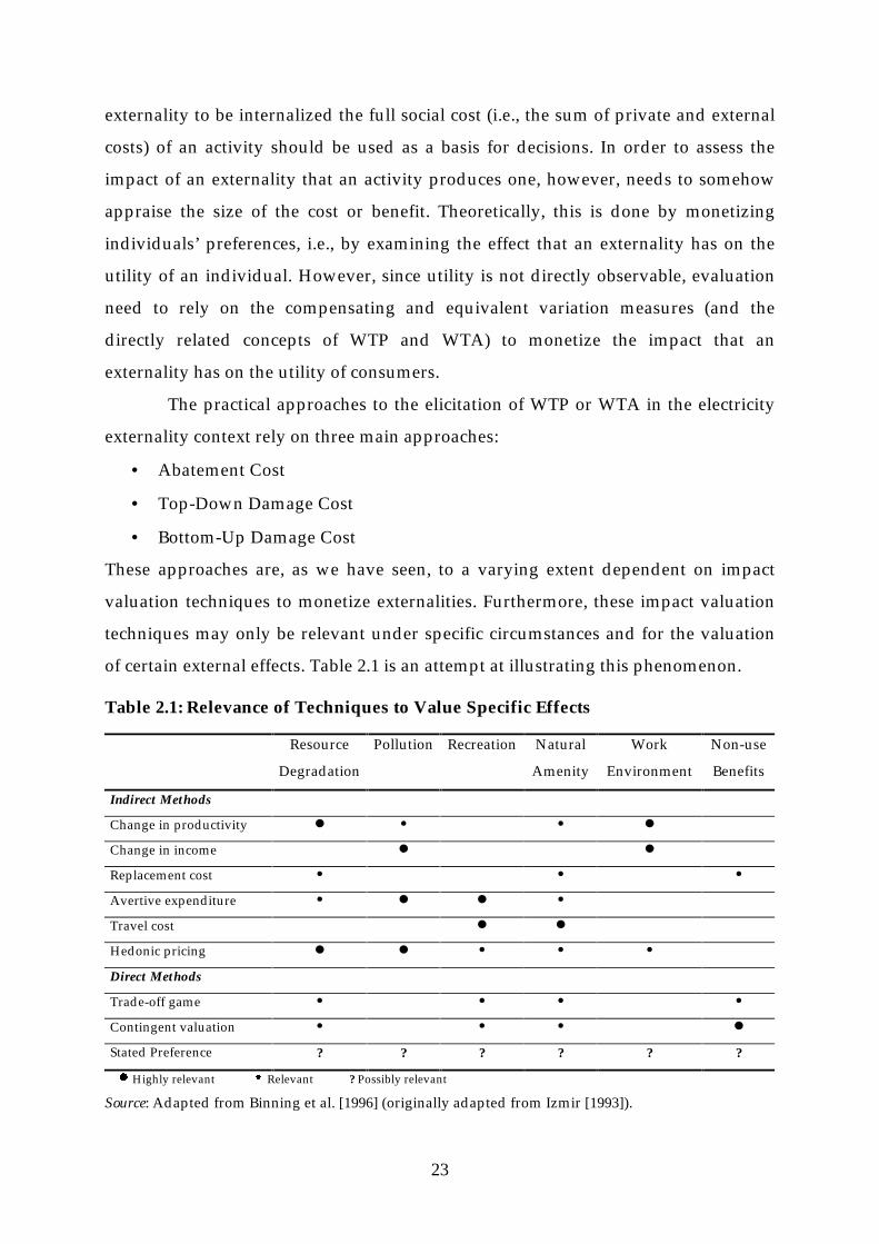
of certain external effects. Table 2.1 is an attempt at illustrating this phenomenon.
Table 2.1: Relevance of Techniques to Value Specific Effects
Resource
Degradation
Pollution Recreation Natural
Amenity
Work
Environment
Non-use
Benefits
Indirect Methods
Change in productivity � � � �
Change in income � �
Replacement cost � � �
Avertive expenditure � � � �
Travel cost � �
Hedonic pricing � � � � �
Direct Methods
Trade-off game � � � �
Contingent valuation � � � �
Stated Preference ? ? ? ? ? ?
n Highly relevant i Relevant ? Possibly relevant
Source: Adapted from Binning et al. [1996] (originally adapted from Izmir [1993]).
24
As table 2.1 indicates the various monetization techniques are only to some
extent relevant in the monetization of specific impacts and, what is more, the
simultaneous use of several methods in the assessment (i.e., to capture the full
impact of an externality) may give rise to double counting.
To conclude, this chapter has provided us with a theoretical foundation in
welfare theory and an abundance of methods to approach the specific problem of
monetizing externalities. These methods may, as table 2.1 indicates, only be useful
under specific circumstances and for specific externalities. What complicates things
further is that the types of externalities that arise from various forms of electricity
production also differ (see chapter 3). Thus, one method may not capture all of the
impacts of an externality and, since the types of externalities differ among fuels,
different methods may have to be utilized in the monetization of impacts for the
variety of fuels. This is especially a problem if, as indicated in this chapter, different
methods tend to yield different results. If this is the case, it may be hard to draw
reliable conclusions about the ranking of different fuel sources in terms of external
costs.
To, clarify some of the issues raised here and to identify and illustrate the
problems of monetizing the externalities arising from electricity production the next
chapter will critically review a representative sample of the studies that have been
carried out during the 1980s and 1990s.

25
Chapter 3
VALUATION OF ELECTRICITY EXTERNALITIES:
A CRITICAL SURVEY OF EMPIRICAL STUDIES
3.1 Introduction
Several studies during the last two decades have addressed the problem of valuing
externalities arising from electricity production. The general purpose of these studies
has been to guide policy makers, i.e., provide a basis for new regulations and ensure
rational choices between different power generation technologies. However, for this
to be possible the methodologies chosen must be used in a reliable manner and in a
way that produces comparable results. In the studies carried out the methodologies
applied have varied immensely, even if there over time has been a growing
consensus towards the (bottom-up) damage cost approach. As we have seen in
chapter 2, different methods bring forth different problems, and maybe also different
externality estimates. Furthermore, some methods may only be useful in specific
situations and for specific fuel sources. The assumptions underlying each
methodological approach also differ. At the same time different fuel cycles cause
different types of externalities. The purpose of this chapter is to illustrate how
externalities from electricity generation can be assessed and what are the
(methodological and practical) problems of doing this. This is achieved by a
thorough review of five influential studies that all have been carried out during the
last two decades.
The reviewed studies together make up a representative sample of the
different methodologies that can be used to assess production externalities, the
sources studied, the countries where externality costing has been attempted, and
hence of the electricity externality studies that have been carried out. The first study
appraised in the chapter, Hohmeyer [1988], is one of the first comprehensive studies.

26
It utilizes the top-down damage cost approach to derive externality estimates for ‘all’
fuel sources. The second study addressed, Bernow and Marron [1990], and Bernow et
al. [1991], uses the abatement cost approach. It derives externality estimates from the
costs implied by regulations (i.e., regulatory revealed preference) for air emissions
arising from fossil fuel burning in two regions in the US. The third study, Carlsen et
al. [1993], makes use of the ranking presented in the Norwegian Master Plan for
Water Resources to derive implicit external costs for potential hydroelectric
developments (i.e., as revealed by decision makers in the ranking). The study is,
hence, also of the revealed preference type. The fourth study reviewed is the
ExternE-project [EC, 1995a-f]. It is probably one of the more influential studies; the
core project has now been followed up by a national implementation program that
utilizes the methodology developed in each of the countries in the European
Community. The methodology used in the ExternE-project is of the bottom-up
damage cost type. In this chapter the sub-studies focusing on coal and hydropower
will be assessed. The final study that is discussed in this chapter, van Horen [1996], is
also of the bottom-up damage cost type and it is the only study included in the
review that focuses on a developing country (South Africa). Table 3.1 presents the
assessed studies in a systematic way.
Table 3.1: Overview of Reviewed Externality Studies
Study Country
(Region)
Quantification
Method
Sources Reviewed
in this Chapter
Comment:
Hohmeyer [1988] Germany
(West)
Damage Cost
(top-down)
Fossil Fuels
Nuclear
Solar (PV)
Wind
‘Cost-Benefit Analysis’ to
determine the economic
effects of replacing fossil
fuels with renewables
Bernow and Marron
[1990] & Bernow et al.
[1991]
US
(Northeast & Southern
CA)
Abatement Cost Coal
Oil
Natural Gas
Only addresses impacts
from air pollutants
Carlsen et al. [1993] Norway Revealed Preference Hydro Valuation based on
Norwegian Master Plan for
Water Resources
EC [1995c & f] Coal: UK & Germany
Hydro: Norway
(EU)
Damage Cost
(bottom-up)
Coal
Hydro
ExternE core project
van Horen [1996] South Africa Damage Cost
(bottom-up)
Coal
Nuclear

27
The review serves as a basis for the assessment of the divergence of
externality estimates as produced by various externality studies in the 1980s and
1990s that follows in chapter 4. Hence, the discussion of studies carried out below
can aid in identifying important differences among the studies that will be of
assistance in explaining the variability of estimates. Furthermore, the review shows
that a direct comparison of studies is rather complex; they differ both in scope (e.g.,
Hohmeyer’s study looks at the economic consequences of replacing fossil fuels with
renewables while most studies only focuses on the costs and benefits of externalities)
and with respect to the specific types of externalities on which they focus (e.g.,
because of his choice of scope Hohmeyer includes avoided external costs of fossil
fuels as a benefit for the renewables, something that is not done in the ‘traditional’
externality studies).
The chapter proceeds as follows. In section 3.2 each of the five studies are
presented and discussed, and they are briefly compared in section 3.3. Finally,
section 3.4 provides some concluding remarks.
3.2 Five Representative Externality Studies21
Several earlier reviews have critically assessed the studies carried out on externalities
arising from electricity production (see OTA [1994], EIA [1995], Martin [1995],
Freeman [1996], Lee [1996 & 1997], Ottinger [1997] and Stirling [1992, 1997 & 1998]).
The focus in the review below will be on the methodologies used, the problems (and
possibilities) encountered in the application of these, the impacts included and
excluded (the reasons for this), and also on the (size of the) estimates produced. Each
section in the review below is divided into two parts; first the study is described and
then briefly discussed and assessed.
21 All monetary estimates presented in this chapter are for ease of comparison expressed in US Dollars
(USD). If the monetary estimates in the reviewed studies were originally in other currencies the
official exchange rates between the local currency (e.g., Deutsch Marks, South African Rands, and
Euros) and the USD have been used to convert them, all estimates have also been recalculated into
1998 prices using the US Consumer Price Index.

28
3.2.1 Hohmeyer [1988]
This study attempts to systematically quantify and monetize the external effects of
electricity production from wind and solar energy and compares these with
electricity produced from fossil and nuclear fuels. The study utilizes the top-down
damage cost approach and focuses on the Federal Republic of Germany. Three
general classes of external effects are considered in the study:
• Environmental effects.
• Economic effects (e.g., employment effects).
• Subsidies (indirect/direct).
Several types of external costs, albeit identified, are not monetized in the study.
These include some human-health related impacts, climatic change impacts and
biodiversity losses as well as all intermediate impacts in the fuel chain (i.e., impacts
arising from other fuel stages than generation). The reasons for the problems in
deriving estimates for these types of impacts are in most cases lack of data and
uncertainties in how to quantify the specific effects. The problems in deriving
estimates were generally higher for the renewables, i.e., solar and wind, than for
fossil fuels and nuclear, something that according to the author places the
renewables at a relative disadvantage.
For fossil fuels Hohmeyer identifies air pollution (SOx, NOx, CO, CO2, PM,
VOC)22 as the primary sources of environmental damages to air and indirectly
through secondary effects to soil and water.23 Any effects from noise or heat are
excluded as they are judged as being negligible. To be able to derive impact estimates
for these air pollutants and ascribe these to fossil energy, Hohmeyer calculates a
relative damage factor for electricity generation from fossil fuels (i.e., the share of
damages specifically due to electricity generation from fossil fuels). This damage
factor was established to be 28 percent for (West) Germany and it was based on
annual emissions from fossil plants weighted with the toxicity factors (e.g., 1.0 for
CO (toxicity basis) and 125 for NOx) of these emissions. The damage factor is then
22 SOx is Sulfur Oxides, NOx: Nitrogen Oxides, CO: Carbon Monoxide, CO2: Carbon Dioxide, PM:
Particulate Matter, and VOC: Volatile Organic Components. 23 These include damages attributable to flora, fauna, humans, materials, and climate.

29
multiplied with total quantified damages (national damage estimate) to identify the
share of these costs that are due to fossil fuel generation (e.g., if total annual damages
are estimated to be 1 million USD, then the annual damage directly attributable to
fossil fuel combustion would amount to 280 000 USD).
Starting with the environmental damages from air pollution, the author
begins by investigating the impacts to plant life (i.e., flora). Hohmeyer notes that the
assessment of these specific impacts are hindered by the fact that air pollution
damages are hard to separate from other natural influences such as climate change,
and that synergetic effects not directly due to air pollution do occur. The monetary
value developed to capture flora damages is based on estimated annual forest and
agricultural crops damages. The minimum range for fossil fuel-caused damage to
flora presented in the study is 1180-1770 million USD per year. Animal life (fauna) is
also affected by air pollution (e.g., acidification of water and its effects on fish stocks).
Here Hohmeyer notes that there exists relatively little earlier research to base fauna
specific damage estimates on, making estimated cost more uncertain. For fauna
impacts he relies on one earlier study, which estimates damages and derives the
share due to fossil fuel power plants to be (at least) 19 million USD annually.
Air pollutants further affect human health. For these impacts Hohmeyer bases
his calculations on estimated air pollution induced costs of respiratory diseases
(morbidity and mortality impacts) from SO2 emissions. This gives a possible range
for fossil fuels of 310-7870 million USD each year. Air pollutants arising from fossil
fuel combustion also cause corrosion and weathering of materials. What complicates
calculations here, according to the author, is that the impacts explicitly due to air
pollution may be hard to isolate and that synergetic effects may exist. For the
estimation of damage costs for these impacts Hohmeyer relies on estimated air
pollution damages developed in the literature. This gives a range ascribable to fossil
fuels of 430-760 million USD per annum. For climate change impacts (from CO2)
Hohmeyer starts by noting that developing cost estimates for these impacts is more
uncertain than for any other type of impact and that the state of research at the time
of study makes the estimated costs very tentative. The discounted average annual
costs for climatic impacts caused by fossil fuels that are presented in the study
amount to approximately 14-27 million USD. This estimate is based on estimated

30
costs of avoiding damage due to flooding (caused by a sea level rise resulting from
global warming) by increasing the height of coastal defense works such as dams,
locks etc. Thus, the total environmental costs from fossil fuel generation derived in
the study then sums to roughly 1960-10450 million USD every year, which
corresponds to 0.08-4.24 US cents per kWh of generated electricity.
So-called environmental impacts for nuclear power generation are also
monetized in the study, i.e., radiation impacts from a major accident. The total
estimate (only human health impacts are considered) presented in the study is based
on estimated Chernobyl accident damages, recalculated to be representative for
German conditions (nuclear and population characteristics) and for various
probabilities of accidents.24 The ‘minimum’ damage range derived by Hohmeyer then
gives an estimate of 0.84-8.36 US cents per kWh of nuclear power production.
The first of the renewables assessed in the study is solar power
(photovoltaic). Identified environmental impacts for solar include land use and
human health. For valuation Hohmeyer uses estimated costs drawn from the existing
literature. For health effects (i.e., maintenance accidents) these rely on income losses
for injuries and years of active working life lost in fatal accidents (net domestic
production per working person and year is assumed to be 35000 USD). Land use
impacts are monetized using opportunity costs (estimated as 10 percent of real estate
price). The resulting total environmental costs for solar power production amounts to
0.31 US cents per kWh. For wind energy Hohmeyer identifies noise impacts as the
only relevant monetizable environmental damage from generation. In order to assess
these previously unvalued impacts ‘first estimates’ are derived in the study, based on
estimated reductions in annual rental values in the proximity of wind turbines,
producing external environmental costs for wind power generation of 0.0006 US
cents per kWh.
After deriving environmental cost approximations for all included fuel
sources Hohmeyer turns his attention to subsidies in different forms. The first
‘subsidy’ considered is natural resource depletion. In order to calculate depletion costs
Hohmeyer relies on a model applying a surcharge based on the concept of backstop
24 Only costs for cancer incidents are included, not health care and psychosocial costs.

31
technology (to be used as an ‘expensive’ substitute to the depleted resource).25 The
model results for fossil fuels (coal, oil and natural gas) give an estimated surcharge of
1.60 US cents per kWh, and for the uranium-based nuclear power production the
surcharge is 4.11-4.32 US cents per kWh. The second subsidy-like externality is
governmentally supplied goods and services (so-called ‘public provisions in kind’), e.g.,
controlling or mitigating schemes publicly provided but privately caused (i.e.,
indirect subsidies). These impacts comprise two main types. The first type relate to
public conservational programs such as public disaster provisions (nuclear subsidy
estimated to be 0.03 US cents per kWh) and public expenditure for pollution
administration and control systems (giving estimates of 0.0002 and 0.0003 US cents
per kWh for fossil and nuclear fuels respectively). The second type involves public
expenditure for general services such as costs of publicly provided infrastructure (in
the study representing a subsidy of 0.44 US cents per kWh for both fossil and nuclear
power generation). Direct monetary subsidies to power producers also ‘constitute’
external impacts in the sense that if there are no external benefits to internalize
through subsidies they distort market outcomes. German public subsidies directed
towards fossil and nuclear power production (either in the form of direct monetary
transfers or as tax reductions) are estimated by Hohmeyer to be equivalent to
external costs of 0.22 and 0.10 US cents per kWh for the two fuels respectively. Public
R&D transfers are according to Hohmeyer the main source of financing new energy
systems and can be considered external if they go uncompensated in markets. For
wind and solar power R&D transfers gives a cost range of 0.18-0.36 and 0.36-0.72 US
cents per kWh respectively. R&D transfers provide subsidies amounting to 0.03 and
1.64 US cents per kWh for fossil and nuclear energy in that order.
Finally, the study also addresses the possible external benefits of renewable
energy production. The first concerns net economic effects, i.e., positive external effects
of increased employment directly attributable to new solar or wind power. These
25 Hohmeyer argues that natural resource depletion constitutes an externality because market prices
do not adequately reflect the increasing scarcity of resources and markets poorly represent the
interests of future generations. Consequently, governments should intervene to ensure long run
optimal resource allocation. The failure to do so, he claims, is effectively subsidizing the resource
depleting technology.

32
benefits are calculated using input-output analysis as domestic net benefits (e.g.,
increased gross value added and lowered public unemployment expenditures) per
year. The computations in the study give external benefits in the range of 0.37-0.65
and 2.06-4.63 US cents per kWh for wind and solar respectively. Additional benefits
of renewables, Hohmeyer argues, are the avoided external costs from the existing
energy system (i.e., from fossil fuels and nuclear). These avoided costs are estimated
as the average weighted gross external costs of fossil fuel and nuclear power
generation. This translates into benefits of approximately 3.73-8.28 US cents per kWh
for the renewables solar and wind.
The discussion above is summarized in table 3.2, which also provides
estimated total externalities.
Table 3.2: Externalities Quantified and Monetized in the Hohmeyer Study
Source
Monetized Impact Cost Estimate
US cents/kWh
Benefit Estimate
US cents/kWh
Fossil Fuels Environmental effects 0.08-4.24
Depletion surcharge 1.60
Governmentally supplied goods 0.44
Monetary subsidies 0.22
Public R&D transfers 0.03
Aggregate: 2.37-6.53
Nuclear Environmental effects (health) 0.84-8.36
Depletion surcharge 4.11-4.32
Governmentally supplied goods 0.47
Monetary subsidies 0.10
Public R&D transfers 1.64
Aggregate: 7.17-14.89
Wind Environmental effects (noise) 0.0006
Public R&D transfers 0.18-0.36
Economic net effects 0.37-0.65
Avoided external costs 3.78-8.28
Aggregate: 0.18-0.36 4.15-8.93
Solar Environmental effects 0.31
Public R&D transfers 0.36-0.72
Economic net effects 2.06-4.63
Avoided external costs 3.78-8.28
Aggregate: 0.68-1.03 5.84-12.91
Source: Hohmeyer [1988].

33
When looking at these estimates one notes the large costs derived for the
‘traditional’ fuel sources, fossil fuels and nuclear (‘worst’ case 6.5 and 14.9 US cents
per kWh respectively) in comparison with the renewables for which the external
benefits exceed external costs. This implies that the consideration of externalities for
the covered fuels would be particularly advantageous for the renewables solar and
wind. The estimates for the fossil fuels and nuclear are dominated by environmental
effects and the depletion surcharge (amounting to between 70.8 and 89.4 percent of
the total). In the valuation of impacts for the first of these (environmental effects) the
uncertainties for both ‘fuels’ are reportedly considerable, leaving many impacts un-
assessed (e.g., global warming). This has probably produced downward biased
externality estimates. The classification of the latter (natural resource depletion) as an
externality is certainly questionable. Some researchers do not even consider the
depletion of non-renewables to be a problem, i.e., markets will left on their own solve
the problem (as scarcity increases costs will go up making further extraction
unprofitable). Additionally, Hohmeyer relies on the concept of ‘backstop-technology’
in the development of external costs for this ‘impact’. This concept is based on the
notion that prices will increase over time, as the non-renewable resource becomes
more scarce (compare with the so-called Hotelling-rule), up to the point to when the
substitute (backstop) technology becomes more attractive. However, actual prices for
non-renewables have, due to technological developments and increased prospecting
etc., fallen over time, thus, in direct contrast to the expected development (i.e., as
assumed by Hohmeyer), indicating decreasing scarcity and that the backstop
technology is not likely to ever become economically viable (see also Radetzki [2000]
for more on this issue). Furthermore, Mäler [1997] when discussing the possibilities
of taxation of non-renewable resources (i.e., as a way of internalizing externalities)
concludes that most tax regimes will only have distorting effects on non-renewable
resource usage, hence implying that markets will often do at least as good a ‘job’ of
solving resource use problems when left to their own.
For the renewables wind and solar the estimated costs are small in direct
comparison. This is at least in part as can be expected; notable however is that
human health impacts (i.e., maintenance injuries) are only considered for solar. The
estimated external benefits for solar and wind as noted above by far exceeds

34
estimated costs. Most of this discrepancy is however due to the so-called avoided
external costs (wind and solar) and the economic net employment benefits (solar).
The first of these (avoided externalities) does not per se constitute an externality.
Including the ‘avoided’ externalities of fossil fuels also gives rise to double counting
(i.e., as an external cost for fossil fuels and as an external benefit for the renewables)
of externalities for these fuel sources [Lee, 1997]. In addition, the inclusion of
employment benefits as an externality in the study strains the definition of what an
externality is (what about lost employment in the fossil and nuclear industry?). In
other words, as Bohi [1993, p. 14] concludes in his paper on non-environmental
externalities: “the existence of a breakdown in the local labor market is required to
establish the existence of an externality, where for some reason unemployed labor
will not migrate to other areas to gain employment, and will remain unemployed
unless there is an increase in local job opportunities.” Consequently, for employment
effects to be considered ‘external’ the local and regional labor market must be
functioning poorly (i.e., market failures must be present) and workers must be
immobile.
Judging the Hohmeyer study as a whole one must note that the scope of this
study is somewhat different than that of ‘traditional’ externality studies, which
focuse on the development of externality adders for different fuel sources, not as
Hohmeyer on judging the economic effects of replacing the present fossil fuel based
generation technologies with more environmentally benevolent renewables. Hence,
what Hohmeyer tries to accomplish is more in line with ‘cost-benefit analysis’ than
with pure externality assessment. Within such a framework, it is correct to include
avoided externalities on the benefit side of the analysis for the renewables. This does,
nevertheless, not make the classification of avoided externalities of fossil fuels as an
externality correct. Consequently, the presentation of cost and benefit estimates in
the study should have distinguished between those cost and benefits that can be
considered external and those that cannot, thus, clearly kept the different types of
costs and benefits separate as not to understate or exaggerate damages and lead
decision-makers astray. Furthermore, the scope of the study makes it hard to
compare Hohmeyer’s results with those of other studies that focus, exclusively, on
externalities.

35
3.2.2 Bernow and Marron [1990], and Bernow et al. [1991]26
This study, which was performed by the Tellus Institute in Boston, relies on the
abatement cost approach. All externality values are derived based on regulatory
revealed preference (i.e., implicit from existing and proposed regulations) or, as it
also may be stated, on the costs of the marginal control technology.27
The study focuses exclusively on air emissions from fossil fuel combustion in
two regions in the US, Southern California and Northeastern US. However, specific
estimates per kWh of produced electricity are only provided for the Northeastern
states; Southern California is consequently left out of the review below. The authors
derive estimates for environmental costs of electricity generation attributable to the
following air quality affecting pollutants:
• Nitrogen Oxides (NOx);
• Sulfur Dioxide (SO2);
• Particulates (TSP/PM10);
• Volatile Organic Components (VOC/ROC);
• Carbon Monoxide (CO);
• Carbon Dioxide (CO2);
• Methane (CH4); and
• Nitrous Oxide (N2O).
Of these only the first five pollutants were regulated under federal and state
standards at the time of the study, while the last three pollutants were not
specifically regulated. These latter pollutants were, according to the authors,
included in the study because they comprise the ‘principal’ greenhouse gases.
Consequently, the regulatory revealed preference approach was only directly
applicable to the first five pollutants for which regulations existed. For the
26 Bernow and Marron [1990] develop cost estimates for the air pollutants (i.e., costs per unit of
pollutant) in their Tellus Institute report; these are attributed to fossil fuel sources and converted into
external cost estimates (per kWh) in the article by Bernow et al. [1991]. 27 A marginal control technology can according to Bernow and Marron [1990, p. 4] be defined as; “the
highest (or marginal) cost [pollution] reduction strategy required by the regulations.”

36
greenhouse gases the developed cost estimates had to be based on assumed future
levels of regulations.
The first study [Bernow & Marron, 1990] addresses the problem of deriving
external cost estimates per unit of pollutant. Starting out with the NOx emissions
Bernow and Marron note that these are regulated under the federal National
Ambient Air Quality Standards (NAAQS) that establish allowable ambient
concentrations for several of the pollutants addressed in the study (NOx, SO2, PM,
and CO). Using the concept of Best Available Control Technology (BACT) the
authors treat the installment of selective catalytic reduction (SCR) as the marginal
technology used to lower NOx emissions in order to meet the NAAQS. Thus, Bernow
and Marron estimate the costs of installing SCR and divide these with the reduction
in emissions to establish the marginal cost of NOx reduction. Based on these
calculations regulators in the US Northeast require NOx control technologies with
costs of at least 8500 USD per ton of pollutant (or 4.2 USD per pound). The next
assessed pollutant, SO2, is also regulated under the NAAQS. For SO2 the authors use
the costs of installing scrubbing equipment to establish marginal control costs, giving
approximately 1970 USD per ton (or 0.99 USD per pound) as cost estimates for SO2
reductions in the (entire) US.28 Particulates (in this case TSP) are covered by the
NAAQS. Bernow and Marron rely on the estimates developed by Chernick and
Caverhill [1990]. Chernick and Caverhill’s estimates of satisfying existing standards
amounted to approximately 5260 USD per ton (2.63 USD per pound) of pollutant.
These figures were based upon the cost of using electrostatic precipitator technology
to increase control from 95 to 99.9 percent at high sulfur coal plants with low
resistivity fly ash. VOCs are regulated under the NAAQS as a reference standard to
control ozone (O3) emissions.29 The developed cost estimates for VOCs are 6970 USD
per ton (or 3.49 USD per pound) of emissions. These values are conservatively based
on the estimated costs of controlling VOC emissions in two other studies, one for the
28 The authors compare their developed cost estimates with the (at the time) pending acid rain
legislation that included emissions trading for SO2 emissions. Recommendations for this system called
for permits to be available at approximately 1970 USD per ton of pollutant, corresponding exactly to
the developed cost estimates. 29 VOCs and NOx interact to form O3 when exposed to sunlight.
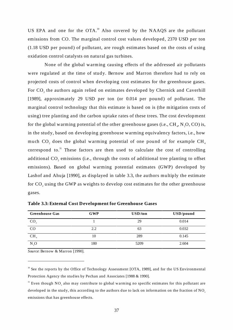
37
US EPA and one for the OTA.30 Also covered by the NAAQS are the pollutant
emissions from CO. The marginal control cost values developed, 2370 USD per ton
(1.18 USD per pound) of pollutant, are rough estimates based on the costs of using
oxidation control catalysts on natural gas turbines.
None of the global warming causing effects of the addressed air pollutants
were regulated at the time of study. Bernow and Marron therefore had to rely on
projected costs of control when developing cost estimates for the greenhouse gases.
For CO2 the authors again relied on estimates developed by Chernick and Caverhill
[1989], approximately 29 USD per ton (or 0.014 per pound) of pollutant. The
marginal control technology that this estimate is based on is (the mitigation costs of
using) tree planting and the carbon uptake rates of these trees. The cost development
for the global warming potential of the other greenhouse gases (i.e., CH4, N2O, CO) is,
in the study, based on developing greenhouse warming equivalency factors, i.e., how
much CO2 does the global warming potential of one pound of for example CH4
correspond to.31 These factors are then used to calculate the cost of controlling
additional CO2 emissions (i.e., through the costs of additional tree planting to offset
emissions). Based on global warming potential estimates (GWP) developed by
Lashof and Ahuja [1990], as displayed in table 3.3, the authors multiply the estimate
for CO2 using the GWP as weights to develop cost estimates for the other greenhouse
gases.
Table 3.3: External Cost Development for Greenhouse Gases
Greenhouse Gas GWP USD/ton USD/pound
CO2 1 29 0.014
CO 2.2 63 0.032
CH4 10 289 0.145
N2O 180 5209 2.604
Source: Bernow & Marron [1990].
30 See the reports by the Office of Technology Assessment [OTA, 1989], and for the US Environmental
Protection Agency the studies by Pechan and Associates [1988 & 1990]. 31 Even though NOx also may contribute to global warming no specific estimates for this pollutant are
developed in the study, this according to the authors due to lack on information on the fraction of NOx
emissions that has greenhouse effects.

38
All the developed cost estimates in the study are compared with the results
of other studies, this to discuss the level and appropriateness of the developed
estimates (i.e., to place own estimates into context). Generally the study’s estimates
compare well with those of other studies, but there are some differences (both higher
and lower estimates are produced by other studies). The authors however deem their
own estimates to be more correct than those of other studies. This since their
estimates are the most recent and that they consequently have been able to evade
most of the problems of earlier studies and also since they have been able to include
the most recent regulations. Bernow and Marron also identify issues for further
research (i.e., possible areas of uncertainty in the development of their estimates) for
all cost estimates. In general it can be said that they recommend that all estimates
should be revised as new legislation becomes available and that the uncertainty of
estimates especially for unregulated and uncontrolled pollutants may be
considerable.
In the follow-up article [Bernow et al., 1991] the developed air pollution
estimates are attributed to fossil fuel combustion (i.e., coal, oil and natural gas), and
converted into external cost estimates per kWh of generated electricity. This is done
using a hypothetical electricity system modeled after the fossil fuel portions of the
New York and New England power pool systems but with added gas capacity. All
data, such as for example heat rates and emissions coefficients (i.e., pound of
emissions per kWh of generated electricity), underlying the simulation are based on
the New York State Energy Plan. The external cost estimates (per kWh) for each plant
considered are then derived by multiplying each plant’s emission coefficients
(pounds per kWh) by the set of emission values (USD per pound) as developed in the
first study. This gives the external costs (low to high) of air emissions per kWh of
generated electricity for each considered fuel presented in table 3.4.
Any careful examination of these estimates is not possible due to the lack of
specific details concerning the actual calculations carried out in the study. However,
given the uncertainties in the derivation of the results, the task of decision-makers,
i.e., too chose what fuel to use when expanding a nations electricity capacity, is not
made any easier by relying on the produced estimates in this study (all ranges
intertwine).

39
Table 3.4: Externalities Quantified and Monetized in the Bernow et al. Study
Source
Aggregate Estimate
US cents/kWh
Coal 5.57-12.45
Oil 4.40-12.89
Natural Gas 2.10-7.98
Source: Bernow et al. [1991].
With regards to the methodology chosen in the study, it is, as discussed in
chapter 2, imperative that the pollution reduction strategy that is used as a basis for
externality costing is the one that gives the least cost of emissions control, i.e.,
abatement cost will only be representative of damage cost when it is derived from
the least cost strategy [Joskow, 1992]. Basing the abatement cost calculations on any
other pollution reduction strategy than the least cost option will hence lead to
external cost estimates that exaggerate the true damages. It does not seem like the
authors have fully accounted for this fact in their study. For example, the costs for
installing scrubbing equipment used for the derivation of SO2 damages need not be
the minimum cost solution. The authors themselves compare the developed cost
estimates with the estimated prices on emission permits (1970 USD per ton), given
this estimate their calculations seems reasonable. However, the actual prices of SO2
emission permits for most of the period 1992-1997 varied between 100 and 200 USD
per ton of pollutant [Schmalensee et al., 1998], indicating that the installment of
scrubbing equipment has not been a least cost alternative and, thus, that the authors
estimates are too high. In practice, the coal plants have instead chosen to rely on low-
sulfur coal in their production as a mitigation measure. Furthermore, as noted by
Smith et al. [1998, p. 23] “estimates in the range of $1000 per ton or more have always
been for the marginal costs, i.e., costs associated with the most difficult-to-control
sources. That narrow focus overlooks the flexibility made possible through emissions
trading.” The failure of the authors (and the abatement cost approach in general) to
identify the least cost solution will, hence, tend to produce estimates that are higher
than those of other approaches. Comparing the damage estimates developed in this
study with those of Hohmeyer (as well as ExternE and van Horen), keeping in mind

40
that only the impacts of air pollutants are considered here, indicates that this is the
case. The aggregated damages are clearly higher than those developed for fossil fuels
in Hohmeyer’s study and (as we will see) also than the damage estimates that the
two other studies have derived (e.g., compare tables 3.2, 3.4, 3.9, and 3.11).
Joskow [1992, p. 61] also questions the consistency in the application of the
revealed preference approach, when discussing the development of damage
estimates for CO2 and for which no regulations existed he remarks: “in the case of
CO2, we have no state or federal regulations governing emissions. As a result, the
revealed preference theory should yield an adder value of zero for CO2 emissions.
Nevertheless, proponents of the cost of control approach have managed conveniently
to put the revealed preference theory aside when it came to making up numbers for
CO2 adders.” Hence, applying the abatement cost approach to arrive at external cost
estimates for impacts for which no regulations exists, as Bernow and Marron do for
CO2, is theoretically inconsistent. Using ‘projected regulations’ as a basis for
derivation is not in line with the abatement cost approach; there are simply no costs
of control on which to base estimates when there is no control.
Another methodological critique, also raised by Joskow [1992], concerns, as
discussed in chapter 2, the tautology of the revealed preference approach, i.e., that
estimates need to be revised every time regulations change (this is one of the
conclusions of Bernow and Marron). Why bother with developing cost estimates that
constantly need to be revised as regulations change, and do the developed damage
estimates at all relate to existing plants? Thus, do the abatement cost approach at all
measure damages that can be transferred to actual power plants? What is more, if
regulations already can be considered to fully reflect the external costs of a
productive activity, are then not the external costs already internalized? Thus, the
external costs are no longer external.
3.2.3 Carlsen et al. [1993]32
This study makes use of the Norwegian Master Plan for Water Resources, which
ranks 542 possible hydroelectric projects with respect to the desirability of future
32 Also discussed in Hervik et al. [1985], Hervik et al. [1986], Wenstøp and Carlsen [1988], Carlsen et al.
[1991], and Carlsen et al. [1992].

41
development, in order to elicit implicit external costs as revealed by the decision
makers in the formulation of the Master Plan. Hence, the methodology chosen sorts
under the revealed preference approach.
The ranking in the Master Plan is based on a number of attributes for which
impacts are described and evaluated. These attributes are assessed for all projects
covered in the Master Plan. The attributes include: Expected Capacity and Regional
Economic Impacts, and User Interests, i.e., impacts that affect:
• Nature Conservation,
• Recreation,
• Wildlife,
• Fish,
• Water Supply,
• Cultural Sites,
• Agriculture and Forestry,
• Reindeer Herding,
• Water Quality,
• Prevention of Flooding and Erosion,
• Ice Formation and Water Temperature,
• Transportation, and
• Climate.
In the Master Plan discrete scores ranging from –4 (‘worst’ case) to +4 (‘best’ case) are
assigned to each of the user interests. The resulting ranking is used for classifying the
projects into 16 priority groups, ranging from more suitable for development to less
suitable for development.
The Carlsen et al. study utilizes the Master Plan and applies regression
analysis to identify the implicit valuations attached by Norwegian decision makers to
the user interests and that are revealed through the decision process underlying the
Master Plan. The regression model gives priority groups as a function of project size,
production costs and binary variables related to regional economic impact and the
user interests. The model can be expressed as follows:

42
( ) ikkjk
RRj
icipi eDbDbP/CbPbbPrjijjij+∑∑+∑+++= 0 (3.1)
where Pri is the priority of a given project i, Pi is the size of project i, (C/P)i is the cost
per unit of expected output for project i, DRji and Dkij are binary variables related to
regional economic impacts and the scores given to the k user interests respectively,
and ei is an error term. The authors specifically note that the model assumes that all
worst-case scores (i.e., -4) are given the same monetary valuation in relation to
projected project output. This is a problem since the actual implicit valuation
attached by decision makers to a worst-case outcome can vary among projects. The
model is nevertheless estimated using ordinal logistic regression and is tested for
robustness using ordinary least squares.
Some of the user interests were excluded from the estimation. According to
the authors, preliminary estimations showed no systematic effect on priority from
the scores attached to water quality, prevention of flooding and erosion, ice
formation and water temperature, transportation, and climate. The results of the
estimated model show that higher priority has been assigned to projects with
favorable regional economic impacts and lower production costs. All estimated
coefficients for the user interests are negative, corresponding to external costs. The
estimated model allowed for calculation of willingness to pay (WTP) to avoid
impacts for each included user interest. More specifically, the decision makers’
revealed willingness to pay can be calculated as the ratio of the estimated coefficients
for Dkj and C/P, or:
ck bbEECj
−= (3.2)
which gives the (implicit) expected external cost (EEC) to avoid development per
unit of output. The resulting externality estimates show that ‘worst’ case scores (i.e., -
4) are associated with implicit costs of roughly 0.9-6.2 US cents per kWh, and scores
of –3 correspond to costs about half this level. Summing up the total external cost for
all considered user interests gives a range of approximately 2.7-26.3 US cents per
kWh. Table 3.5 gives more detailed information on the external cost estimates

43
produced for each user interest within the study as well as on the scores that were
ascribed values.
Table 3.5: Estimated External Costs in the Carlsen et al. Study
User Interest Range of Scores with Attributed
Costs
Expected External Costs
(US cents/kWh)
Nature Conservation (-2)-(-4) 0.328-3.216
Outdoor Recreation (-2)-(-4) 0.642-2.600
Wildlife (-2)-(-4) 0.246-0.942
Fish (-1)-(-4) 0.077-3.098
Water Supply (-1)-(-4) 0.297-6.181
Cultural Monuments (-1)-(-4) 0.577-2.825
Agriculture (-2)-(-4) 0.246-4.612
Reindeers (-1)-(-4) 0.266-2.786
Aggregate: 2.679-26.260
Source: Carlsen et al. [1992].
For the preferred projects total external costs corresponded to approximately
70 percent of production costs and for all projects about 160 percent of production
costs. It is concluded that the extra costs (i.e., to protect sites found least suitable for
development) that this ranking imposes on Norwegian consumers amounts to
approximately 10-130 USD per household and year.
The results also allow the derivation of a long-run marginal cost curve for all
ranked projects. This curve was mostly rising, but not uniformly so. This may,
according to the authors, be due to model specification errors and/or inconsistencies
in the actual ranking (i.e., the final ranking is not fully consistent with the implicit
valuations attached by decision makers to the user interests). These problems may
produce biased estimated coefficients and thus biased externality estimates.
The statistical approach to the assessment of external costs utilized in this
study provides some interesting possibilities. Even if no such comprehensive
appraisal of possible hydroelectric sites as the Norwegian Master Plan exists in other
countries there may be other types of ‘rankings’ from which implicit values may be
elicited. When examining the actual external cost estimates it is however worth
nothing that the range of estimates and consequently the uncertainties in the
interpretation are considerable. This may be due to the problems reported in the
44
study, i.e., that the ranking is not representative of the implicit values attached to
each site by decision makers, and hence to some extent questions the applicability of
the approach. Furthermore, the methodological approach in this studies suffers from
the same circularity problem as mentioned earlier (see the discussion of Bernow and
Marron’s study above), i.e., the constant need for revisal of estimates as new
legislation (regulatory preferences) becomes available questions the applicability of
the approach in the power generation context.
3.2.4 European Commission [1995c & f]
Initiated in 1991 this study is part of a major ongoing project, known as the ExternE
project, within the European Community. The core-project reports, primarily aimed
at developing an externality accounting framework for each fuel cycle and an
appropriate methodology within which to assess energy related externalities, were
published in 1995 [EC, 1995a-f].33
All studies in the project utilize the bottom-up damage cost approach, here
known as the impact pathway. The analysis begins by identifying the range of the
burdens and impacts that result from the fuel chain and defining the technologies
under investigation. It then assesses the priority of impacts. The impacts that are
deemed to have insignificant effects, based on the magnitude of impacts, are
excluded from the assessment. The significant impacts are then quantified using data
that is relevant to each specific situation. The quantified impacts are then monetized
based on individual’s willingness to pay using the methodology appropriate for the
particular circumstances.
Given the wide scope of the ExternE-project, i.e., ‘all’ energy sources, (and
the sizeable reports) the review below will focus exclusively on the coal and hydro
studies. These are included to represent one ‘traditional’ fuel (coal) and one
‘renewable’ (hydro). Furthermore, the specific methodology applied within the
33 The national implementation program that applies the developed methodology on the EC-countries
was finalized in late 1997 to early 1998 (see Appendix 1). The reports from the national
implementation program will not be addressed here (they will however be covered in chapter 4).
Efforts to develop methods for aggregation of results so to make them useful for policy makers were
also included in the national implementation program.

45
ExternE hydro sub-study deviates somewhat from the standardized assessments
within the ExternE-project.
Coal
The ExternE coal sub-study [EC, 1995c] looks at two different sites, one in the UK
(West Burton ‘B’) and one in Germany (Lauffen), both of which had been identified
as suitable for new coal capacity.34 Both plants are assumed to rely on the same
power generation technology (electrostatic precipitation) and both stations are to be
fitted with flue gas desulfurization (FGD) that reduces SO2 emissions by
approximately 90 percent. Other emission standards are however less restrictive in
the UK than is the case in Germany. For example, according to the authors German
legislation implicitly requires the use of more effective NOx-reduction technology
(selective catalytic reduction) as compared to UK regulations (low NOx burners).
Consequently the assumed emission levels for NOx from the two plants differ
considerably. The emission levels used as a basis for damage costing in the study are
summarized in table 3.6.
Table 3.6: Assumed Air Pollutant Emission Levels in the ExternE Coal Study
Pollutant West Burton, UK Lauffen, Germany
(grams per kWh of produced electricity)
Carbon Dioxide (CO2) 880 880
Sulfur Dioxide (SO2) 1.1 0.8
Nitrogen Oxides (NOx) 2.2 0.8
Particulate Matter (PM) 0.16 0.2
Source: EC [1995c].
The ExternE coal study addresses all stages of the coal fuel cycle, i.e., from
the construction of the plant and the mining for coal, the generation and transmission
of electricity, the disposal of waste produced, and finally to the decommissioning of
the plant. However, overall more attention has, according to the authors, been given
to the power generation stage.
34 In the study the coal power plants were modeled to have a peak capacity of 1800 MW (West Burton)
and 700 MW (Lauffen) respectively.

46
To ‘properly’ assess the atmospheric dispersion of air pollutants arising from
the coal fuel cycle the study relies on models tracing pollutant dispersion and
transformation in the atmosphere that were developed within the ExternE-project
and by other European research institutes (see the methodology report, EC [1995b],
for details). This, according to the authors, represents an important modelling
breakthrough in comparison with earlier externality costing studies focusing on
fossil fuels. The following main groups of impacts from the coal fuel cycle were
deemed by the authors to lead to significant external costs and are hence prioritized
in the study:35
• atmospheric pollution impacts on human health (public and occupational),
• occupational and public accidents,
• atmospheric pollution impacts on materials, crops, forests, fishery and ecosystems,
• global warming impacts,
• noise impacts, and
• coal mining impacts on water quality, and on buildings and constructions.
The air pollutants from the coal fuel cycle that affects public health identified
as significant in the study are PM and ozone (O3).36 The impacts from these emissions
are quantified using dose-response functions relating daily variation in pollution
exposure to health impacts (i.e., morbidity and mortality impacts). Examples of dose-
response functions employed for the assessment of PM impacts on health in the
study are presented in table 3.7.
Table 3.7: Dose-Response Functions Employed by the ExternE Coal Study
Public Health Impacts from Particulates
Response Unit Estimated Function
Mortality % change in rate 0.104
Morbidity Symptom/day/person/year 0.050
Chronic shortness of breath Days/asthmatic/year 0.140
Source: EC [1995c].
35 According to the authors the selection of priority impacts is based on an extensive literature review,
expert opinions and discussions within the research team. 36 Impacts from SO2 and NOx emissions on public health are indirectly considered in the study as they
contribute to PM formation and NOx alone to the formation of O3.

47
According to the authors, these dose-response relationships are subject to
considerable uncertainties. For example, they mention that there is a ‘legitimate
debate’ on the relevance of the different pollutants, the transferability of dose-
response functions and on the applicability of these functions in different situations.
Monetization of mortality impacts from air pollution in the study relies on the value
of a statistical life (VSL) approach, producing estimated damages for mortality
impacts in the study of 0.45 US cents per kWh for West Burton and 1.42 US cents per
kWh for Lauffen.37, 38 Chronic and acute morbidity effects from air emissions were
valued using estimated WTP to avoid different symptoms.39 This gives total impacts
of approximately 0.05 US cents per kWh and 0.38 US cents per kWh for each plant
respectively. Transport accident impacts are assessed for the West Burton plant only.
These were quantified using national statistics on road traffic accident rates and
valued using UK estimates on the costs of minor and serious accidents.40 The total
estimated health damages for the coal fuel cycle in the study then amount to roughly
0.5 US cents per kWh for the UK site and 1.8 US cents per kWh for the German plant.
The large differences between the two estimates are reportedly mainly due to the
geographical area considered for each site. Health damages from West Burton are
limited to the UK while impacts from Lauffen were calculated for all of Europe.
There is however another difference between the two estimates; ozone related
impacts on mortality and morbidity were assessed only for Lauffen.
Occupational health impacts that arise from the coal fuel cycle include air
pollution impacts on coal miners (i.e., radon and dust) as well as accidents during
mining, limestone quarrying, transport, construction and operation. The
37 The VSL value adopted in the ExternE-project, approximately 3.6 million USD, is derived based on a
review of earlier VSL studies in Europe (primarily carried out in the UK). 38 The estimated function (e.g., 0.104 for mortality impacts from PM) is basically multiplied with the
VSL to arrive at total damage cost for each pollutant impact. 39 This WTP value was derived from a review of US literature; reportedly to little research on the
issued had been carried out in Europe. This, according to the authors, can be a bit problematic since
the direct transferability of results from the US to Europe may be questionable. 40 The ranges used in the study are: roughly 600-5000 USD for minor accidents, and 39000-310 000 USD
for major accidents. These ranges are calculated using typical accident rates in the coal fuel cycle and
monetized using the VSL-value assumed in the ExternE-project.

48
quantification of radon impacts on miners relies on measured doses of radon
received by miners. Using these data the study estimates that radon induced lung
cancer will cause roughly 0.02 deaths among coal miners per TWh in the UK and 0.06
deaths per TWh in Germany. Monetization for radon impacts rely on the VSL-
approach and the estimated damage costs are 0.007 US cents per kWh for West
Burton and 0.02 US cents per kWh for the Lauffen plant. Dust impacts on miners are
quantified using typical dust levels at European coal mines.41 The disease rates are
estimated at 0.1 persons per TWh in the UK and 0.3 persons per TWh in Germany,
the lower value for the UK reflecting the higher productivity in UK coal extraction.
The average fatality rates for the persons with these types of lung diseases are
estimated using UK data to be 0.21 percent. Hence, estimated mortality damages are
0.008 US cents for the West Burton site and 0.02 for the Lauffen plant. Accident
impacts (i.e., fatalities and injuries) are quantified using national statistics on accident
rates (assessed for coal mining, limestone quarrying, transport, construction and
operation) in the study. The monetization of occupational accident impacts is based
on the same UK cost estimates for minor and severe accidents that were used to
assess public accidents. Accidents in mining are the dominant category for both
plants; estimates are however considerably higher for Lauffen (e.g., 0.5 deaths per
million tones mined and 0.07 US cents per kWh) than for West Burton (e.g., 0.2
deaths and 0.03 cents). According to the authors, this difference is mainly attributable
to the better safety record in the UK coal industry. Total accident damages dominate
the occupational health impacts giving estimates of roughly 0.1 US cents per kWh
(UK) and 0.3 US cents per kWh (Germany) for this category.
Materials, such as building surfaces, are also affected (e.g., by corrosion) by
air pollutants arising from the coal fuel cycle. The main factors here are according to
the authors’ direct SO2 emissions and acidic deposition.42 For corrosion effects the
analysis focuses on the costs of repair and maintenance of materials used in buildings
41 Dust releases in the mining of coal cause various respiratory diseases such as fibrosis. 42 Acidic deposition, or ‘acid rain’, is primarily caused by sulfur emissions omitted into the atmosphere
that together with oxygen forms sulfur dioxide, and by nitrogen oxides (i.e., any compound of
nitrogen and oxygen). Both of these pollutants mainly arise from fossil fuel combustion [Swedish
Environmental Protection Agency, 2000].

49
(i.e., neglecting any effects of aesthetic nature and on materials used for other
purposes than building; this reportedly due to problems in quantifying these
impacts). The building material impacts assessed were quantified using dose-
response functions relating the amount of pollution to corrosion damages on
surfaces. The repair costs were assessed by estimating the change in the frequency of
maintenance caused by atmospheric pollution. In the study acidity was assessed for
the whole of Europe (for both sites). SO2 emissions were, however, only modeled for
all of Europe for the Lauffen plant. The assessment of the West Burton facility only
considered SO2 effects within the UK. The resulting increase in building repair costs
attributable to acidification and SO2 emissions amount to 0.11 US cents per kWh for
West Burton and 0.03 US cents per kWh for Lauffen. This difference is reportedly
mainly due to variations in the inventories used in the quantification. For the UK site
cleaning costs due to PM-emissions were also assessed. The quantification and
monetization of these impacts relied on PM-emission data from coal power plants in
the UK (adjusted for soiling efficiency) and the size of the UK building cleaning
market. This approach neglects any trans-boundary impacts as well as the effects of
plant location. The increases in cleaning costs due to PM-pollution from UK coal
power plants amount to 0.006 US cents per kWh.
Air pollution from coal combustion also affects agricultural production (i.e.,
crops), mainly through the formation of SO2 (direct and indirect effects) and by
contributing to the formation of O3 (only considered for the German site). The direct
effects of SO2 pollutant impacts are quantified in the study through the use of dose-
response functions as identified in the European literature. These were however
(wherever deemed to be relevant) adjusted for the (positive) fertilizing effects of
sulfur. The dose-response relationships used for West Burton relied on two basic
sources, first a meta-analysis of several earlier rye grass studies, and secondly on a
single study of barley yields near the site. For Lauffen dose-response functions
derived from German experimental work on crop damages were used. Impacts were
assessed for the major cereal crops.43 The quantification relied on existing data on
43 For West Burton the analysis covered wheat and barley, and for Lauffen impacts on wheat, barley,
oats and rye were considered.

50
crop yields and land use. The results in the study show that average yields changes
by less than 1 percent even in the proximity of the plants, but since the total area
affected is large, the annual losses due to each plant on average amount to more than
2000 tons of cereal. In the study these calculated losses are valued at international
market prices producing damage estimates of approximately 0.003 US cents per kWh
for both sites. The study also includes a ‘first attempt’ at assessing O3 impacts, using
the same methodological approach as for SO2 impacts. The resulting estimates
amount to 0.00005 US cents per kWh for the Lauffen plant. Here the authors point
out that there were too little research available to derive reliable damage estimates,
and that the damage estimates calculated therefore should be considered as very
preliminary. For the West Burton site acidic deposition impacts were also assessed.
These impacts were appraised as the additional amount of lime needed to counteract
acidification evaluated at market prices. This gives a monetary estimate for the UK
power plant of roughly 0.0006 US cents per kWh of produced electricity. Several
potentially significant crop impacts were according to the authors not considered in
the analysis due to problems in identifying earlier research on which to base dose-
response relationships. These excluded impacts include synergetic effects between
different pollutants and between pollutants and pesticides, as well as damages to
high value crops (e.g., vegetables, fruits and flowers). As a consequence the total
reported damages (0.004 and 0.003 US cents per kWh for West Burton and Lauffen
respectively) may, as the authors emphasize, only represent a ‘low’ estimate of the
true damages on agriculture as caused by coal-based power production.
The atmospheric pollutants arising from coal power plants also affect forests.
The assessment of forest damages in the coal study mainly focuses on acidity effects;
the appraisal for the Lauffen plant however also considers O3 damages. Acidification
impacts from Lauffen are quantified using dose-response relationships, relating
observed damage and critical load exceedance for acidity, applied on Norwegian
spruce on acid soils in Germany. The study estimates that emissions from the
Lauffen plant would significantly damage 1000-2000 hectares of forest over a five-
year period. Mitigation measures necessary to avoid these impacts would, according
to the calculations in the study, correspond to a cost of roughly 0.001 US cents per
kWh. A similar methodology was used in the study to evaluate local O3 damages

51
from the Lauffen plant. This gave damage estimates of 0.00003 US cents per kWh. For
the UK implementation the assessment of effects of acidity on forests relies on a
slightly different approach. Here the study employs relationships between critical
loads and tree crown conditions, and crown conditions and tree growth to estimate
timber losses attributable to the West Burton plant throughout Europe. The
calculated physical timber losses were then valued at market prices giving a damage
cost of 0.0006 US cents per kWh. The authors also note that several potentially
important impacts could not be considered in the assessment of forestry impacts.
These include all direct impacts of nitrogen on timber production, as well as impacts
on little known forest functions such as soil stabilization, carbon retention,
biodiversity etc. For these reasons, they conclude, the valuation attempts are only
partial.
Noise amenity impacts from the coal fuel cycle were only assed for the UK
plant in the study. The impacts considered here adhere to public amenity losses from
the power production and transportation stages, neglecting any noise disamenities
from other stages in the fuel cycle (e.g., coal mining) and any health related effects of
noise pollution. The noise impacts from (road and rail) transport are quantified based
on data from an Environmental Impact Assessment previously carried out on the
West Burton site. The Environmental Impact Assessment gives expected changes in
noise levels due to increases in rail and road traffic. The authors, using
measurements from an existing coal power plant, calculate power station noise
levels. The analysis in the study also considers the dispersion of noise over the
relevant population, i.e., along transportation routes and in the vicinity of the power
plant. The monetization of noise impacts is based on estimated reductions in housing
values in the affected areas. The values used are primarily based on a review of
hedonic pricing studies of road and airport noise carried out in Europe and the US.
The noise-related damages from the West Burton plant are estimated to amount to
0.02 US cent per kWh. According to the authors uncertainties affecting the
interpretation of this estimate mainly include the applicability of road and airport
studies to the present case, how to deal with noise reductions in natural
environments, and the response of individuals to increasing levels of noise.

52
The only aquatic impact quantified and monetized within the study is acidic
deposition. This impact is assessed in the study by looking at lime usage to preserve
water quality in Norway and Sweden. In total approximately 35 million USD was
spent on mitigating acidification impacts on rivers, streams and lakes through the
use of lime in these two countries in 1990. The study quantifies acidic deposition
attributable to the two plants by calculating the proportion of sulfur and nitrogen
deposition in Norwegian and Swedish waters that can be directly ascribed to the
power stations. Multiplying these estimated proportions with the actual expenditure
on liming gives estimated damages of 0.0002 US cents per kWh for West Burton and
0.001 US cents for Lauffen. The study also quantified impacts on freshwater fisheries
due to air pollutants from the coal fuel cycle for parts of the UK and reviewed other
research on the issue; however no monetary estimates were derived. Other aquatic
impacts (e.g., coal mining impacts and emission impacts on recreational fisheries)
were discussed in the study but no quantification and monetization was attempted,
this due to lack of data.
Global warming impacts from the coal fuel cycle are extensively analyzed
within the study but the authors report that a full assessment of impacts from the
power plants considered are beyond the scope of the study. Using earlier research
the study however derives damage estimates for global warming as presented in
table 3.8. These are, according to the authors, not to be considered as estimates for the
project but rather as the result of a literature review (and as an illustration of the
problems and huge uncertainties associated with the assessment of global warming).
They specifically report the following problems with valuing global warming
damages based on earlier research:
• considerable differences in ethical judgments (e.g., choice of discount rates)
and assumptions,
• incompleteness in details in the studies,
• large uncertainties in the estimation of impacts, and
• ignorance of the likelihood of synergies between effects.

53
Table 3.8: Global Warming Damage Estimates for the Coal Fuel Cycle
Source on which based Discount rate
(%)
Estimate based on Damage estimate
(US cents/kWh)
Cline [1992] 0 US damage 2.1
Fankhauser [1993] 0 US damage 1.4
Tol [1995] 1 US damage 2.6
Hohmeyer & Gärtner [1992] 0 Global damage 700
Source: EC [1995c].
Reportedly the relatively close agreement between the first three estimates
arises due to a commonality of assumptions. These studies are not, however, based
on a more ‘solid foundation’ than the assumptions adopted by Hohmeyer and
Gärtner [1992]. Based on the review of the studies covered in table 3.8 the authors
conclude that even if the assessment of global warming impacts are inherently
difficult, the impacts are likely to dominate most other impacts from the fossil fuel
cycles.
Ecosystem damages due to air pollution, habitat destruction etc. have also
been reviewed but not quantified and monetized within the study. The authors note
that the damage cost potential may be substantial but that even if quite a lot of earlier
research exists on the issue, monetization using the partial dose-response
relationships that could be identified was not possible. The authors conclude that
valuation of impacts on ecosystems at present is too complex a task, and hence that
for the ‘foreseeable future’ such valuation exercises will probably not be possible.
In their assessment the authors end by addressing the manifold of other
impacts from the fuel cycle left out of their current analysis but that may be of
significant magnitude. These include visual amenity impacts, visibility reductions
due to pollution, impacts of thermal discharges etc. These impacts are reportedly not
fully known and therefore call for further examination.
Table 3.9 summarizes the discussion above and presents aggregate estimates
as well as the reported uncertainties in the calculation of these.

54
Table 3.9: Externalities Quantified and Monetized in the ExternE Coal Study
Monetized Impact Fuel Stage Quantification Basis Monetary Basis Uncertainty Total Estimate
US cents/kWh
Public health Generation
Transportation
Air emissions: PM & O3 (G
only): Dose-response
functions
Accidents: National
accident rates
Air emissions: Mortality:
VSL Morbidity: Benefit
transfer (WTP to avoid
different symptoms)
Accidents: Benefit transfer
Medium-High 0.54 (UK) & 1.82 (G)
Occupational health Mining
Quarrying
Construction
Generation
Transportation
Air emissions: Diseases
(Radon): Estimated data,
Dose-response functions
Accidents: National
accident rates
Air emissions: Mortality:
VSL Morbidity: Benefit
transfer (WTP to avoid
different symptoms)
Accidents: Benefit transfer
Low-High 0.11 (UK) & 0.32 (G)
Materials Generation Air emissions: SO2 &
acidification: Dose
response functions PM:
Emission data
Air emissions: SO2 &
acidification: Repair costs
PM: Cleaning costs
Low-High 0.11 (UK) & 0.03 (G)
Agriculture Generation Air emissions: SO2 , O3(G
only) & acidification(UK
only): Dose response
functions
Air emissions: SO2 & O3:
Crop losses evaluated at
market prices &
acidification: Mitigation
costs
Medium-High 0.004 (UK) & 0.003 (G)
Forestry Generation Air emissions: O3 (G only)
& acidification: Dose
response functions (G) &
physical timber losses (UK)
Mitigation costs (G) & Market
prices (UK)
High 0.0006 (UK) & 0.001 (G)
Amenity Generation
Transport
Noise Benefit transfer High 0.02 (UK)
Aquatic Generation Air emissions:
Acidification: Estimated
SO2 & NOx emissions
Mitigation costs Medium 0.0002 (UK) & 0.001 (G)
Aggregate: 0.86 (UK) & 2.25 (G)
Legend: G Lauffen, Germany
UK West Burton, UK
Source: EC [1995c].
A quick examination of the results in the ExternE coal study reveals that (if
one disregards the CO2 component) the aggregate externality estimate for both sites
is dominated by the impacts on human health (75.6 and 95.1 percent of total for the
UK and German site respectively). Other impacts (except material impacts for the UK
plant) seem to have a significantly smaller impact. Striking is also the reportedly high
uncertainties in the development of most of these cost estimates. This questions the
reliability of the estimates. As noted by the authors, in the development of externality
estimates many possibly significant impacts had to be left out of the analysis. This
has most certainly produced external costs that, given that the reported estimates are

55
correct, underestimate the true externalities arising from the coal fuel cycle. There
also seems to be an overall unwillingness to develop dose-response relationships for
impacts that are hard to quantify and monetize (i.e., for which little earlier research
exists) in the study. The possibility of the results presented in the study being
downward biased increases when one considers that no monetary estimate is
included for global warming impacts, keeping the rough calculations done within
the study in mind (see table 3.8). There is a danger of leaving impacts of this
apparent magnitude unmonetized in a study as influential the ExternE project. A
casual examination of the results in the study may lead policy makers to draw
inaccurate conclusions on the advantageousness of the coal fuel cycle when
contemplating future expansions of the energy sector.
Worth noting is also that the estimates derived in the ExternE coal study are
very low in comparison with earlier studies of coal that have been reviewed earlier in
this chapter. One might suspect that this, at least in part, is related to the choice of
methodology (i.e., bottom-up damage cost versus top-down and abatement cost).
Hydro
As reported in EC [1995f] the hydropower sub-study in the ExternE core project
focuses on an expansion of the existing hydroelectric scheme in Sauda, Norway. The
following impacts are prioritized in the study:
• Agriculture;
• Forestry;
• Water supply;
• Ferry traffic;
• Recreational activities;
• Cultural objects;
• Terrestrial and aquatic ecosystems;
• Occupational health;
• Regional and national economic impacts; and
• Bird populations.
All of these impacts are quantified in the study and all but one (bird population
impacts) are monetized. The impacts on bird populations are however, according to

56
the authors, partly included in the assessment of the impacts on terrestrial and
aquatic ecosystems. The methodology applied relies on the standard ExternE
methodology briefly discussed above. However, in contrast to the other fuel cycles
covered in the ExternE-project the valuation of impacts have not relied on general
dose-response functions. This since, according to the authors, the impacts arising
from the hydro fuel cycle are more direct in comparison with for example fossil fuels
from which impacts are mostly indirect (i.e., emissions), but also more project- and
site-specific. The authors have therefore had to rely heavily on the development of
impact estimates based on expert estimates from the Environmental Impact
Assessment of the Sauda scheme. Expert estimates from this Environmental Impact
Assessment were used in the calculation of impacts on agriculture, forestry, water
supply, ferry traffic, recreation, objects of cultural and archeological interests, and
also of impacts on aquatic, terrestrial and marine ecosystems (i.e., biodiversity).
The quantification of occupational health effects during construction was based
on actual accident rates in the Norwegian construction sector (12 deaths and 2691
injuries annually). These data were transformed to be representative of expected
accident rates at the Sauda project. The statistics were monetized using the VSL-
approach and estimated injury costs.44 Operational accidents from routine operations
(disasters were not included) were quantified using accident data (i.e., injuries and
deaths) specific for the Norwegian hydroelectric sector. These data were monetized
using the same values as for construction impacts. This gives an estimated damage
from occupational health effects of 0.005 US cents per kWh.
Agricultural impacts were quantified as the area of lost grazing land. This
impact was valued using the cost of renting equivalent grazing land elsewhere also
adding any incurred transportation costs (i.e., replacement costs). The estimated
monetary impact for agricultural impacts of Sauda development is then 0.0014-0.0015
US cents per kWh. Forestry production damages from the Sauda project were in the
study quantified as the area that has to be clear-cut due to rock waste dumps, roads
etc (no forest areas will be inundated). The derived costs were calculated as net
44 The following approximate numbers were used: 3.6 million USD for a loss of a statistical life (VSL),
39000-310 000 USD for major injuries, and 600-5000 USD for minor injuries.

57
revenues from lost future forest production of birch minus net revenues from cutting
the present stand, relying on birch market prices and productivity data to monetize
impacts.45 This amounts to an estimated damage range of 0.00001-0.00006 US cents
per kWh for forestry impacts.
Damages to water supply (as caused by the estimated reduced flow of water)
are valued using replacement costs (e.g., costs of new wells and improvements of
irrigation systems) as identified in the Environmental Impact Assessment. The
resulting external cost estimates are 0.00048-0.00189 US cents per kWh. The discharge
of temperate water from the project will prevent ice formation and make it possible
for the ferry company in the Sauda Fjord to operate all year round (ferry benefits). The
benefits from this are calculated as the net reduction in operating costs (i.e., avoided
buss rental costs), adding benefits for the passengers due to reduced travel time and
avoided inconvenience costs both valued using the opportunity cost of time (value
based on an estimated WTP of 6-10 USD per hour of reduced travel).
Employment benefits are estimated using a method developed in the study that
elicits values based on the government’s preferences for creating new jobs and the
cost of job creation. Specifically, local employment effects were calculated using
subsidy rates per man-year and national employment effects were valued using the
costs of creating jobs through expansionary government policy using a computer
model. Employment benefits are in the study estimated to be in the range 0.03-0.35
US cents per kWh.
A contingent valuation study was used to value impacts on recreation,
cultural sites, and on terrestrial and aquatic ecosystems. In the CVM-study carried out,
it was assumed that the environmental impacts of Sauda hydroelectric development
were only of relevance to local and regional inhabitants. Thus, a zero-WTP was
assumed for the rest of the Norwegian population. This might, as the authors note,
cause downward biased estimates of the true WTP. The CVM-survey used direct
interviews (i.e., face-to-face questions) performed on approximately 600 respondents
that represents some 13 percent of the local and 1 percent of the regional population.
45 The authors stress the fact that pine that has a higher value than birch also will be affected,
something that probably causes the resulting values to underestimate the true costs.

58
The questionnaire utilized open-ended questions, i.e., what is the maximum amount
you are willing to pay to avoid the specified environmental impacts? The resulting total
WTP amounted to roughly 2.4 million USD per year giving a WTP per kWh of 0.316
US cents for damages to recreation, cultural objects and biodiversity. 46
The resulting externality estimates from the study, and the reported
uncertainties in the calculation of these are presented in table 3.10.
Table 3.10: Externalities Quantified and Monetized in the ExternE Hydro Study
Impact Fuel Stage Quantification
Basis
Monetary Basis Uncertainty External Costs
US cents/kWh
Ext. Benefits
US cents/kWh
Agriculture Construction Area of grazing
land lost
Replacement
costs
Low 0.0014-0.0015 —
Forestry Construction Clear cut area
(birch)
Market prices Low 0.00001-0.00006 —
Water Supply Operation Reduction in
water flow
Replacement
cost
Low 0.00048-0.00189 —
Ferry Traffic Operation Days of
additional
operation
Reduced
operation &
travel costs
Low — 0.00064
CVM aggregate for
recreation, cultural
objects, &
biodiversity
Construction &
Operation
— WTP Medium 0.316 —
Occupational Health Construction &
Operation
National injury
& fatality data
VSL & injury
costs
Medium-high 0.005 —
Employment Effects Construction &
Operation
Number of new
jobs (local &
national)
Local: Subsidy
rates/man
year
National:
MODAG
Not reported — 0.03-0.35
Aggregate: 0.32 0.03-0.35
Source: EC [1995f].
Table 3.10 shows that the CVM-estimate dominates the cost side (roughly 99
percent of total) and employment effects the benefit side. The CVM-study may as the
authors note have derived a WTP-value that underestimates the true value
(producing a downward bias on the aggregate) since the ‘national WTP’ was
46 An estimate of the impacts on recreational activities in the Sauda area already existed before the
CVM-study was carried out. The Environmental Impact Assessment of the Sauda project is based on a
benefit transfer from existing valuation studies estimated recreation values for the Sauda area. These
values were considered by the authors to be too uncertain to use in the present study and they
decided to carry out themselves a CVM-study that was considered to produce more reliable results.

59
assumed to be zero. Moreover, the inclusion of the estimate for employment benefits
is as noted earlier (see the discussion concerning Hohmeyer’s study above) at least to
some extent ambiguous. There is no doubt that the building of a new hydropower
plant will increase local demand for labor, however, for this to be considered an
(positive) externality the plant must give employment to workers that would
otherwise remain unemployed.
As can be expected, the coal damages are considerably higher than those
developed for hydropower. However, the direct comparability of the two studies is
limited due to the fact that the assessed externalities differ considerably. The impacts
from coal mostly relate to ‘easy-to-quantify’ indirect air pollutant damages, while
hydroelectric impacts mostly arise from effects on ecosystem’s etc, for which impacts
are more complex and uncertain (for more on this issue see. Söderholm and
Sundqvist [2000a & b]). For example, in a CVM-study ecosystems are described in a
manner that renders them commodity-like, and there is little room for what we
would normally claim is the most important aspect of an ecosystem – its functional
aspects (e.g., its life-supporting mechanisms). This is in heavy contrast with, say, SO2
emissions, whose impacts (e.g., corrosion) are more tangible and directly connected
to human disutility. The studies, hence, differ with respect to the nature of their
externality appraisal.
3.2.5 van Horen [1996]
The South African study included in the review relies on the bottom-up damage cost
(impact pathway) approach. The objective of van Horen’s study is to develop
estimates for the external costs arising from electricity production in South Africa for
the two dominant fuel sources, coal and nuclear.47 All identified impacts are not
assessed in the study (see further below). The following classification of impacts was
used in the study to determine the scope of the quantification and valuation:
47 As van Horen reports, the national utility Eskom is the predominant producer in the South African
electricity sector. In 1994 it generated 96 percent of all electricity produced in South Africa. At the end
of 1994 the total capacity of Eskom’s power stations amounted to 37840 MW, out of which
approximately 89 percent was coal-fired (12 power plants) and 5 percent nuclear (1 power plant).

60
• Class One impacts; impacts which are considered potentially serious (i.e.,
significant monetary size of impact as compared with the price of electricity is
expected) and for which sufficient information exists to permit economic
valuation.
• Class Two impacts are impacts deemed to be potentially serious, but for which
only insufficient data exist to allow valuation.
• Class Three impacts are impacts judged to be insignificant in relative size as
compared with other impacts from the fuel cycle and/or impacts already
internalized.
Impacts given the Class One classification are consequently quantified and
monetized within the study.
For the coal fuel cycle the following impacts were identified as Class One or
Two impacts in the study:
• Mining: occupational health effects; air and water pollution impacts.
• Power generation: water consumption and quality impacts; air pollution
impacts on health, of acidic deposition and on visibility; and impacts from
greenhouse gas emissions.
Occupational health impacts from mining that are classified as Class One
impacts in the study include mortality- and injury-related impacts. Morbidity
impacts, i.e., respiratory illnesses caused by air pollution, are given Class Two
classification and are thus not quantified in the study, this due to insufficient
information on which to base estimates. This may, as van Horen notes, lead to
externality estimates that will understate the true external costs. The quantification of
occupational health impacts from mining is based on the actual number of fatalities
and injuries in South African mining. The author, relying on actual accident rates,
calculates accident rates for the specific coal mines that supply the coal power plants
of the national utility Eskom. The calculated accident rates used are 0.156 fatalities
(mortality) and 0.874 injuries per thousand GWh of electricity produced from coal in
1994.48 For injuries a low estimate of 4 weeks and a high estimate of 8 weeks of
48 This corresponds to 23 deaths and 131 injuries for coal mined in South Africa and used in Eskom’s
coal power plants in 1994.

61
absence is used for quantification purposes. The valuation of the mortality impacts is
based on the VSL-approach. The actual VSL-value used in this study is based on
income adjusted (to account for the South African income distribution) averages of
the values used in the New York State study [Rowe et al., 1995] and the ExternE
study [EC, 1995a-f].49 This implicitly assumes that these valuations (of VSL) vary in
direct proportion to income. Using the VSL-approach the estimated range of
mortality-related externalities from coal mining in the study is 0.004-0.009 US cents
per kWh. Valuation of injury impacts from coal mining is based on actual costs of
medical treatment, costs of productivity losses (i.e., opportunity costs of not
working) and compensatory payments to injured workers. This amounts to
estimated external costs of 0.0002-0.0007 US cents per kWh. The identified pollution
impacts from mining on air and water were not quantified in the study
(consequently these impacts were attributed a Class Two classification) due to
insufficient information on which to base estimate, and these impacts may also to
some extent, according to the author, already be internalized (Class Three impact)
through existing mitigation schemes.
For power generation the impacts identified as arising from (under-priced)
water consumption of coal power plants are given Class One classification, while
water quality impacts are considered to have insignificant effects in the study and are
thus assigned Class Three classification. The water consumption impact is quantified
using actual consumption and pricing data, the produced estimates in the study are
based on the estimated cost of supplying additional water. This gives an externality
range of 0.003-0.007 US cents per kWh. The health impacts from air pollution
(mortality and morbidity) arising from coal power are classified as Class One
impacts (ash produced by combustion of coal is however not quantified due to lack
of information (Class Two)). According to van Horen, the quantification of health
impacts requires information on:
• the emitted pollution quantities (of PM, O3, SO2, NOx) from power plants,
• the dispersion and deposition of these pollutants, and
• the health responsiveness of humans to these pollutants.
49 The actual VSL-estimates used are a low of 2.9 million and a high of 5.6 million USD.

62
The quantification of pollution quantities in the study is based on estimated
emissions as calculated by Eskom. The quantification of the dispersion and
deposition of pollutants is based on physical characteristics (e.g., height of power
plant chimneys), atmospheric conditions (e.g., wind patterns), and on pollutant
concentration data (e.g., SO2 concentration levels) as calculated by Eskom in the
proximity of one of their coal power stations. The dose-response relationships (i.e.,
between pollution and health) used in the study are based on dose-response
relationships developed within the New York State Environmental Externality
Costing Study [Rowe et al., 1995], or more specifically on the computer model
(EXMOD) developed within the study. The author makes use of the EXMOD-
program to quantify and estimate mortality and morbidity externalities from the coal
fuel cycle. EXMOD is however based on characteristics that are specific to North
American conditions and is only to some extent modified for the environmental and
demographic conditions prevalent in South Africa.50 The use of the model will
consequently, as the author notes, produce biased results (the direction of this bias is
however somewhat uncertain). The valuation of health impacts is for mortality
impacts based on the calculated VSL-value (see discussion above) and for morbidity
on cost of illness data (used in EXMOD computations). The estimated range of health
impacts in the study is 0.158-0.265 US cents per kWh. Acidic deposition and visibility
impacts from air pollution are classified as Class Two impacts in the study, this due
to the lack of data applicable to the South African case. The study also addresses
greenhouse gas emissions in the form of CO2.51 The quantification of these impacts is
based on CO2 emissions data as calculated by Eskom. The monetary valuation relies
on estimated damages per ton of CO2. More specifically, the estimates produced by
the Intergovernmental Panel on Climate Change (IPCC) are used (low estimate 5
USD per ton). Van Horen, however, based on a review of other studies, thinks that
50 The model allows for adaptation of most parameters. Van Horen, however, reports that insufficient
data exist to more fully adjust the model to reflect South African conditions. 51 The author notes that the combustion of coal also gives rise to CH4 that has a relatively higher global
warming potential than has CO2. CH4 is however excluded due to ‘lack of data reasons’ (something
that can lead to an underestimation of the total damage attributable to coal based electricity
generation in South Africa).

63
the IPCC’s high estimate of 125 USD per ton is too high and makes his own
‘arbitrary’ calculation to arrive at a high estimate of 33 USD per ton. The resulting
externality estimates range from a low of 0.699 US cents per kWh to a high of 4.670
US cents per kWh.
All other impacts that were not explicitly addressed in the study (e.g.,
electro-magnetic fields, aesthetics, etc.) were classified as Class Three impacts. The
aggregate value for the South African coal fuel cycle produced by the study then
amounts to 0.897-5.014 US cents per kWh this, van Horen reports, corresponds to 18-
99 percent of Eskom’s average tariffs in 1994.
For the South African nuclear fuel cycle the following potentially significant
(i.e., Class One and Two) impacts were identified in the study:
• environmental impacts and risks (of e.g. radioactive emissions), and
• fiscal externalities.
Of these, only the second category is addressed in the study (Class One impact). Van
Horen reports that even though the environmental impacts and risks are of likely
significance in aggregate, any quantification of these impacts in the South African
context is not possible due to lack of data and time (and scope) constraints on the
study. These impacts are therefore assigned the Class Two category in the study, and
will hence (negatively) bias the total externality estimate. The fiscal externality in
South African nuclear power generation pertains to fiscal subsidies made by
authorities not reflected in the price and which are possibly significant in relation to
the price of electricity.52 The quantification and valuation of this ‘impact’ is based on
the part of the subsidies directly attributable to the production of electricity
(approximately 45 million USD). This total was then ‘spread’ over different scenarios
over the lifetime of the power plant. The low estimate (1.336 US cents per kWh) is
based on the plant operating at full capacity until 2023 while the high estimate (4.543
US cents per kWh) is based on the plant ceasing all operations in 1996. These
estimates correspond to between 2-6 percent of average electricity tariffs in 1994.
52 Indeed van Horen reports that the total fiscal subsidy given to the South African nuclear sector
exceeds 70 billion USD in real terms, while coal-fired generation has received little or no financial
support from authorities.

64
When discussing these estimates van Horen notes that since several
potentially significant impacts were left unquantified and unmonetized in the study,
the aggregated values only reflect minimum (or first) estimates of the ‘true’ external
costs in South African power generation. Van Horen reports the following main
limitations and weaknesses of his study:
• omissions of potentially significant impacts (Class Two),
• uncertainties in the quantification and valuation of Class One impacts, and
• bias on externality values due these omissions and uncertainties.
Table 3.11 summarizes the discussion above, presents the estimated
externalities as well as the reported level of uncertainty associated with the
calculation of these in the study.
Table 3.11: Externalities Quantified and Monetized in the van Horen Study
Source
Fuel Stage Monetized Impact Quantification Basis Monetary Basis Uncertainty Total Estimate
US cents/kWh
Coal Mining Occupational health
(mortality & injuries)
Actual accident rates Mortality: VSL
Injuries: medical costs;
productivity losses; &
compensation payments
Moderate 0.004-0.010
Generation Water consumption Actual consumption &
pricing
Costs of supplying
additional water
Moderate 0.003-0.007
Generation Air pollution & health
(mortality & morbidity)
Estimated physical
emissions; dispersion &
deposition data; & dose-
response functions
(EXMOD)
Mortality: VSL
Morbidity: cost of illness
Moderate 0.158-0.265
Generation Greenhouse gas
emissions
CO2 emissions data Estimated damage/ton of
CO2
High 0.699-4.670
Aggregate: 0.897-5.014
Nuclear Fiscal subsidy Total subsidy to the
South African nuclear
sector
Estimated share of total
subsidy attributable to
nuclear power
production
Moderate 1.336-4.543
Aggregate: 1.336-4.543
Source: van Horen [1996].
An inspection of the aggregated results from van Horen’s study discerns that
the external cost estimate for the coal fuel cycle is dominated by the impacts from
greenhouse gas emissions (between 77.9 and 93.1 percent of aggregate), the estimate
that has the highest reported uncertainty, and hence the greatest reported range. The
results for both fuel cycles must, given the considerable number of unmonetized
65
impacts, be interpreted as significantly downward biased, something that the author
also concludes.
Furthermore, the application of the EXMOD computer model to South
African conditions is not uncomplicated. The problems in adopting the basic model
data as to be representative for the environmental and demographic situation
prevalent in South Africa makes the developed air pollutant emission impact
externalities unreliable. Also, including subsidies (as van Horen does for nuclear) in
the calculations is only correct if one wants to find the ‘true’ total production costs
for a plant (i.e., subtracting these from the ‘private’ costs of the power station), but
subsidies do not constitute externalities. It, thus, seems as if van Horen’s study
(much like Hohmeyer) tries to accomplish something more than just externality
appraisals, something that questions the direct comparability of his results with those
of ‘pure’ externality studies.
3.3 Comparing the Studies
First it may be worth noting, keeping the limited number of studies addressed in this
chapter in mind, that when one looks at the time span of studies there seems to have
been a standardization towards the bottom-up damage approach when addressing
electricity externalities. This may be something that implies a growing consensus of
bottom-up damage costing as being the ‘appropriate’ way of approaching this
problem. It may also be the case that earlier studies, given the present technology
and state of knowledge would have, had they been performed today, relied on this
approach.
Examining all the studies reviewed in the chapter there also seems to be a
general and considerable reliance on the research of others. For the later studies often
on other externality costing studies (see, for example, van Horen above), and thus
little or no original research on which to base estimates. The real danger with this
phenomenon may be that errors (if any) in the original research are inherited if these
data sources are not properly discussed and corrected for sources of error (in the case
of reliance on other externality studies that in turn has inherited their estimates a
further magnification of errors) thus producing biased external effect estimates. It
however seems that major (later) studies such as the ExternE-project (and other

66
studies of the same magnitude not specifically addressed in this chapter) tend to
have to a greater extent developed their own original data on which to develop
externality estimates. Indeed the bottom-up damage approach (impact pathway) is,
as was discussed in chapter 2, relatively more data intensive in the development of
estimates since it sets out to trace impacts all the way from the source.
The ability of the different methodological approaches to capture specific
effects also needs to be scrutinized. Can a case be made that the ability of abatement
cost, top-down damage cost, and bottom-up damage cost differ with respect to this?
In addition, can impacts addressed using these different approaches really be
compared? Looking at the impacts addressed in the Carlsen et al. study it can be seen
that some of the classified impacts (user interests) do not directly correspond to
impacts addressed within for example ExternE hydro study. It may be that the use of
one specific approach to elicit values for externalities may force a type of impact
classification that gives damage estimates that measure something else than the use
of another approach.
Another issue that arises from the comparison of the studies discussed in this
chapter relates to the omission of possibly relevant impacts. This causes underrated
total externalities, producing ‘biased’ implications for corrective policy not in
compliance with the optimal level of externality, i.e., too much of the externality will
be allowed. None of the studies reviewed in this chapter are able to derive monetary
estimates for all identified impacts. This problem is complicated further by, as the
comparison of included impacts in the different studies reveals, the possibility that
the studies may have missed out on identifying other significant impacts.
There is also a danger of at all reporting results that are based on a study that
omits possibly significant results; there may be a tendency for others to treat the
aggregate as representative for the total externality even when the possibly highest
external impact has been left out of the study (e.g., global warming impacts). The
study may thus report a small aggregate but since the impact that ought to be
assigned the highest value has been left out, the interpretation of the aggregate
becomes complicated. For this reason, among others, there are difficulties in
comparing the estimates produced by different studies. What is considered a
possibly relevant impact in one study may also (as we have seen above) differ among

67
the studies. In the study by Hohmeyer for example, natural depletion is considered a
very significant externality arising from the reliance on fossil and nuclear fuels.53 Van
Horen’s study on the other hand does not even consider depletion. This also raises
the question of what is actually considered to comprise an externality in each study.
Should other types of market failures be included in the classification or should
corrective policies (such as public subsidies) that miss their target be included? The
studies thus seem to differ considerably in their definition of what constitutes an
externality (e.g., see discussion above on Hohmeyer’s ‘avoided external costs’ and
the ExternE hydro study’s ‘employment benefits’). This also pertains to the ‘scope-
discussions’ of Hohmeyer’s and van Horen’s studies above. They both, in some
sense, want to do more than just assess externalities. Hence, if a study tries to assess
the ‘true’ production costs, i.e., in line with a cost-benefit analysis, the consideration
of all costs and benefits (internal as well as external) are relevant. This means that a
study that tries to evaluate the effects of replacing the existing electricity structure is
correct in including the benefits of avoiding the damages of the present structure into
the calculations (e.g., Hohmeyer). However, this does not mean that the avoided
damage costs of the present electricity structure (e.g., Hohmeyer) are ‘external’.
Interrelated with the discussion above is the issue of including external benefits into
the analysis. Two of the studies addressed here (Hohmeyer and ExternE) include
benefits in their calculations. This will, if such effects exist and an externality study
simply omits them from consideration, produce positively biased total externality
estimates.
The extent to which the estimated damages and/or benefits can be directly
converted into external costs and/or benefits, i.e., are some of the estimated damages
already internalized, is also an issue of crucial importance. Some of the studies
explicitly address this issue (e.g., van Horen and ExternE) while some of the other
studies do not (e.g., Hohmeyer, Bernow et al. etc). Ignoring any already internalized
impacts gives estimates that exaggerate the external effects of the assessed impacts.
53 As mentioned in the discussion of Hohmeyer’s results above, depletion can hardly be considered an
externality, and in contrast with the assumptions in the study empirical evidence points to decreasing
scarcity (i.e., falling prices on non-renewables over time) indicating that depletion is not a problem.

68
Looking at the size of specific estimates in the studies (this specific discussion
will be developed in chapter 4) one may especially notice the very significant size of
effects for greenhouse gases developed for fossil fuels in the van Horen study where
CO2 damages account for approximately 80-90 percent of the total externality
estimate. When compared with the results of the Hohmeyer-study where these
impacts correspond to approximately 0.1-0.3 percent of total estimate these impacts
may seem high. Both authors however note that the uncertainties in the development
of the global warming impacts are extremely high. Leaving the global warming
impacts out of the comparison of the studies gives another interesting view of the
developed estimates. Disregarding greenhouse gas impacts it seems that the results
of the earlier study by Hohmeyer are significantly higher than those of van Horen.
Furthermore, redeveloped estimates of global warming impacts by Hohmeyer and
Gärtner [1992] are considerably higher than the ones presented in the earlier study
(these global damage estimate range from a low of 290 US cents per kWh for natural
gas to a high of 700 US cents per kWh for coal). The treatment of underlying
uncertainties in the development of externality estimates for global warming impacts
is hence crucial for the total outcome.
Another issue that pertains to the size of estimates is that, as also noted in
OTA [1994], in all considered studies (no matter if greenhouse gases are assessed) a
single category of effects seem to dominate the estimate. For example in Hohmeyer’s
and the ExternE coal study human-health related impacts dominate the aggregate
damage (75.3 percent and 75.6-95.1 percent for each study respectively), but the
dominant impact in one study is not generally the same as in other studies (e.g., in
the ExternE hydro study the impacts on recreation, cultural objects and biodiversity
dominate, and for van Horen CO2 impacts constitute the majority of estimated
damages from the coal fuel cycle). This may indicate that the studies emphasize
impacts inconsistently something that may (further) imply that the comparability
between studies may not be very good (see Stirling [1998] for a more elaborate
discussion of this issue). Thus, if relatively more effort in one study is put into the
development of cost estimates for e.g. air pollution impacts the chance of developing
a bigger estimate might be considerable.

69
Also, a comparison of the Carlsen et al. study and the ExternE hydro study
that both are carried out on the same fuel and in the same country reveals
considerable differences in total estimates.54 The estimate produced in the first study
is some 82 times greater than the estimate in the second. This questions the
comparability of estimates produced by different methodological approaches and
implies that the revealed preference approach (and as we have seen the abatement
cost approach) may fail to approximate the ‘true’ damages. Hence, everything else
held constant, the use of regulatory revealed preference to derive external cost
estimates implies higher aggregated damages than what can be expected from the
(bottom-up) damage cost approach. Thus, this is line with Joskow’s explanation of
this phenomenon, and this reasoning suggests that the choice of methodological
approach might explain some of the variation in results.
What is more, there seems to be considerable differences in basic
assumptions and in the value basis’s used. For example the assumptions about
monetary value of the Value of a Statistical Life differ considerably in the studies
addressed above, the ExternE study uses a VSL-value of 2.6 million USD while van
Horen relies on values of 2.9-5.6 million USD. Hence, the impacts assessed using the
VSL-approach (e.g., human health impacts) will be dependent on the underlying
values used and the assumptions in the different studies will determine the
outcomes.
There are also differences in scope between the studies. Some studies (e.g.,
Hohmeyer and Bernow et al.) only consider the operational phase of the fuel cycle
while others (e.g., ExternE) take into account (all) other stages in the fuel cycle. This
may affect outcomes, i.e., studies that cover the full fuel cycle should, ceteris paribus,
produce higher estimates than studies that only consider generation. This discussion
is also related to the geographical scope taken in the assessment of so-called
‘transboundary’ impacts (see for example the ExternE coal study). Only considering
national damages of air pollutants that spread outside of a nations borders will
produce downward biased estimates.
54 The difference in total estimates is also evident from comparing Bernow et al.’s and ExternE’s
estimates for coal.

70
Noteable is also that the results of the CVM-study performed for the Sauda
hydroelectric project is very significant in comparison with other impacts. The CVM
aggregate comprises almost 99 percent of total estimated damages from the project. If
this is a pattern that repeats itself when other studies attempt to combine CVM
valuation results with other estimates there is some cause for concern. This is clearly
something that we will have to look more carefully into in the next chapter. One
possible explanation of this phenomenon may however be that CVM-studies tend to
produce high estimates because respondents are not liable to actually pay (so-called
‘strategic’ bias). Hence, the stated willingness to pay in a CVM-survey may be
considerably higher than the actual willingness to pay thus in the application in
externality studies producing overestimated damages.
Another striking issue that stands out from the discussion of Bernow and
Marron’s as well as Carlsen et al.’s studies above concerns the circularity of the
revealed preference approaches (e.g., abatement cost), i.e., the constant need for
amending the estimated damages as new regulations are imposed. This makes it
possible to question whether the approach at all can be considered representative for
actual power plants, and also to question if (as is implied by the fact that regulations
already exist) the external costs of a productive activity are already internalized. That
is, why bother with externality appraisal if politicians’ decisions already are optimal?
It is equally important to recognize that the reliance on the revealed preference
approach entails a different ethical basis as compared with the other approaches. For
example, the damage estimates developed within the ExternE-project are considered
ex ante, i.e., the damages themselves determine whether one power source is ‘better’
than another, while the estimates derived using the abatement cost approach are ex
post, i.e., the price is an outcome of a political process and does not play a direct role
in the decision.55 The damages developed in ‘advance’ (as in the ExternE-project) may
therefore not be directly comparable to ‘implicit’ estimates, that relies on the cost of
abating as revealed by decision makers, since they as Söderholm and Sundqvist
[2000b, p. 15] note “reflect different reasoning processes,” this questions the
economic theoretical foundation of the abatement cost approach. For example, policy
55 See Söderholm and Sundqvist [2000a & b] for a more developed discussion on this issue.

71
makers may in their formulation of regulations rely on other ethical foundations than
economic welfare theory. Hence, any discrepancies between the damages estimated
by the different approaches may simply be attributed to the different bases of the
available methodologies and for this reason they may not be directly comparable.
3.4 Concluding Remarks
Based on the review and discussion above, what are the problems and possibilities of
properly assessing electricity generation externalities? To sum up, the following three
main conclusions may be drawn. First, there exist theoretical reasons which support
that the abatement cost approach tends to produce higher estimates in general, thus
implying that there are methodological reasons to the discrepancies in the results of
the various studies. Second, there are several problems in the application of the
various methodologies that may help explain the disparity of estimated damages.
For example, the differences in scope among studies (and methodologies) complicate
the comparison between studies and may, hence, provide important explanations to
the specific problem. Furthermore, some of the studies have included costs (and
benefits) into the calculation that cannot be considered to be externalities. This is due
to the differences in scope; these studies are attempting to assess the ‘full’ cost of the
fuel cycles under consideration (i.e., something above pure externality cost
assessment). Third, the thoroughness of approach differs considerably among the
studies, both when it comes to the specific impacts that the studies consider and
pertaining to the stages in the fuel cycle that are assessed (further complicating the
comparison of studies). For the above reasons previous studies
Finally, before we go on to chapter 4, it must be noted that the illustrative
nature of the review carried out in this chapter is not sufficient to meet the second
purpose of this thesis. Since different fuels cause different external effects in order for
us to be able to delve deeper into the reasons of the divergence of externality
estimates we will need to compare more studies for each fuel. Stirling [1997, p. 531],
in his discussion of the variability of estimates, calls for a more systematic approach
to the issue and concludes that: “[m]ore elaborate statistical treatment might
illuminate such patterns further and reveal correlations with particular aspects of the
methods, assumptions, scope or institutional contexts of individual.” Thus, we will

72
need to actively and systematically compare all identifiable studies for all fuels to
possibly distinguish some general explanations to the differences in magnitude of
estimates. This will, to some extent, reveal whether the choice of methodological
approach and the thoroughness of approach in the different externality studies
affects estimates, and also whether the results can be used in the ranking of different
fuels (i.e., as a basis for policy). This is what the next chapter sets out to do.

73
Chapter 4
EXAMINING THE DISPARITY OF EXTERNALITY ESTIMATES
4.1 Introduction
The main aim of this chapter is to address, and if possible, explain the wide disparity
of results as produced by the different externality studies carried out on the
electricity sector during the 1980s and 1990s. This chapter will address this specific
issue by examining all the studies that have been identified and the results that these
have produced. First, in section 4.2, the results of all electricity studies are described.
In section 4.3, these studies are addressed qualitatively, compared and scrutinized.
After that an attempt at quantifying the analysis using a statistical technique called
ANOTA (ANalysis Of TAbles) that resembles linear regression analysis, but all
variables (dependent as well as independent) are categorical is made. ANOTA is
applied to all studies in section 4.4. Finally, the main conclusions of the chapter are
summarized in section 4.5.
4.2 Overview of Electricity Externality Studies
There have been a number of electricity externality studies carried out in the 1980s
and 1990s. Approximately 40 different electricity externality studies of various fuel
sources have been identified in the literature (see Appendix 1). All monetary
estimates in these studies have, for ease of comparison, been converted into US
Dollars and into the 1998 price level using official (mean) exchange rates and the US
Consumer Price Index. Originally the estimates were presented in various currencies
and in un-equivalent ‘sizes’, such as for example German Pfennigs (1/100 Marks)
and US Mills (1/1000 USD). This process has not always been uncomplicated, mainly
because the base year for the monetary estimates presented in the respective studies
are not always explicitly expressed. Whenever this problem arose, the year of
publication was used instead as a proxy for conversion. This may have lead to

74
somewhat biased externality estimates. As figure 4.1 shows (note logarithmic scale)
the disparity of results between the different studies is considerable.
Min-Max25%-75%Median value
US
Cen
ts/k
Wh
(Log
arith
mic
Sca
le)
0,01
1,00
100,00
COALOIL
GASNUCLEAR
HYDROWIND
SOLARBIOMASS
Figure 4.1: Range of External Cost Estimates for Different Fuel Sources
Sources: Appendix 1.
Looking at, for example, coal and oil the range of results produced by the
studies carried out is from 0.004 to roughly 2000 US cents per kWh for coal and from
0.05 to roughly 680 US cents per kWh for oil. Thus, the highest values for coal and oil
are several thousand percent higher than the lowest estimated value (see also table
4.1). In addition, the ranges presented below, as Stirling [1997] also notes, by far
exceed the ranges presented in any single study and there is also a substantial
overlap between fuel sources. It should be clear that this discrepancy of results will
lead to problems in the ranking of the different options. This pertains to the ‘goals’ of
externality assessment, namely to provide a ranking of fuel options on which to base
decisions of future capacity expansion or formulate efficient environmental taxes. 56
The vagueness in results provided by the studies makes such an ordering of fuels
56 Stirling [1997] also mentions another problem that he calls the ‘price imperative,’ i.e., that there is a
tendency of results to converge around the actual electricity price level, a level that is most useful for
policy-making. That specific issue will, however, not be addressed here.
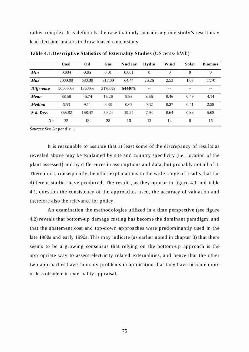
75
rather complex. It is definitely the case that only considering one study’s result may
lead decision-makers to draw biased conclusions.
Table 4.1: Descriptive Statistics of Externality Studies (US cents/kWh)
Coal Oil Gas Nuclear Hydro Wind Solar Biomass
Min 0.004 0.05 0.01 0.001 0 0 0 0
Max 2000.00 680.00 317.00 64.44 26.26 2.53 1.03 17.70
Difference 500000% 13600% 31700% 64440% -- -- -- --
Mean 88.58 45.74 15.26 8.83 3.56 0.46 0.49 4.14
Median 6.53 9.11 3.38 0.69 0.32 0.27 0.41 2.58
Std. Dev. 355.82 158.47 59.24 19.24 7.94 0.64 0.38 5.08
N= 35 18 28 16 12 14 8 15
Sources: See Appendix 1.
It is reasonable to assume that at least some of the discrepancy of results as
revealed above may be explained by site and country specificity (i.e., location of the
plant assessed) and by differences in assumptions and data, but probably not all of it.
There must, consequently, be other explanations to the wide range of results that the
different studies have produced. The results, as they appear in figure 4.1 and table
4.1, question the consistency of the approaches used, the accuracy of valuation and
therefore also the relevance for policy.
An examination the methodologies utilized in a time perspective (see figure
4.2) reveals that bottom-up damage costing has become the dominant paradigm, and
that the abatement cost and top-down approaches were predominantly used in the
late 1980s and early 1990s. This may indicate (as earlier noted in chapter 3) that there
seems to be a growing consensus that relying on the bottom-up approach is the
appropriate way to assess electricity related externalities, and hence that the other
two approaches have so many problems in application that they have become more
or less obsolete in externality appraisal.

76
0
5
10
15
20
1982 1988 1989 1990 1991 1992 1993 1994 1995 1996 1997 1998 1999
Nu
mb
er o
f st
ud
ies
Abatement cost Damage cost (top-down) Damage cost (bottom-up)
Figure 4.2: Methodologies Used in the Appraisal of Electricity Externalities Over Time
Sources: Appendix 1.
Keeping this phenomenon in mind one would expect results, as also noted
by Stirling [1997], to show some clear trend over time, i.e., to converge towards some
reasonable level of divergence. Stirling, in his [1998] article, suggests that a
‘reasonable level’ of divergence that may be explained by site specific conditions, un-
commonality of assumptions etc. may be something like four orders of magnitude.
Looking at the results for fossil fuels over time (see figure 4.3), no such trend
can be distinguished. There seems to be no convergence of externality values as
methodology matures (i.e., towards the bottom-up approach) and as researchers get
more experienced (e.g., learning curve effects). This shows that the variability of
results in the late 1990s tends to be as great as in the late 1980s to early 1990s.
Moreover, this ‘superficial’ analysis further indicates that the bottom-up approach is
as inconsistent in externality appraisal as the other two approaches; abatement cost
and top-down.

77
US
Cen
ts/k
Wh
(Log
arith
mic
Sca
le)
0,01
0,10
1,00
10,00
100,00
1982 1986 1988 1989 1990 1991 1992 1994 1995 1996 1997 1998 1999
Figure 4.3: External Costs from Fossil Fuels Over Time
Sources: Appendix 2.
The remainder of the chapter deals solely with the issue of explaining the
discrepancy in externality estimates. In the next section (4.3), five hypotheses are
formulated. Assessing these will, we argue, provide the main explanations to the
disparity of results. The assessment is done in two steps; first, in section 4.3, the
externality studies are examined graphically and verbally, after that, in section 4.4, an
attempt to systematically test the hypotheses using the ANOTA model is made.
4.3 Why do the Externality Estimates Differ?
The starting point for the following discussion is that addressing the following
specific issues may provide the main explanations to the considerable discrepancy of
externality estimates for a given fuel source:
1. Site and Country Specificity – the impacts will depend on the specific location of
the power plant and so will the externalities that arise (i.e., no direct
comparability and transferability of externality estimates between different
sites or countries is possible).
2. Convergent Validity – different quantification and valuation methods tend to
produce different results (e.g., the estimates produced by the abatement cost
method may be generally higher than the estimates produced by the damage

78
cost method or the values produced by impact valuation techniques such as
the contingent valuation technique may differ from the values produced by
other valuation techniques).
3. Repetitive Validity – the application of quantification and valuation
methodologies in similar contexts may produce different results (e.g.,
contingent valuation results may be affected by bias arising from, for example,
respondents that answer more or less strategically). 57
4. ‘Thoroughness’ – one study may differ from another by simply looking at more
externalities than another (i.e., more monetized impacts would typically lead
to higher total externality estimates) and the estimates would become
especially biased if the omitted externalities are those that are associated with
very high impacts (e.g., CO2 emissions may as we have seen in chapter 3 be an
impact that significantly affect aggregate damages). The issue of thoroughness
is also related to the completeness of approach taken in each of the studies,
i.e., especially when it comes to the specific issue of whether the respective
studies have addressed the full fuel cycle for the plant under study (e.g., from
fuel extraction to the decommissioning of the plant). The more stages in the
fuel cycle that one study addresses the higher the expected total damages.
5. Assumptions – the basic assumptions made in the development of damage
estimates in a study may also affect the size of estimates (e.g., if one study
assumes that the quantitative damage of one impact is higher than in another
study one would expect this study to, everything else held constant, produce
higher externality estimates).
The following sections (4.3.1-4.3.5) will focus on each of these issues; i.e., develop the
discussion concerning each hypothetical explanation and investigate whether they
are of any relevance when it comes to explaining the disparity of externality
estimates. The discussion focuses on fossil fuels, primarily since fossil fuel studies are
the most numerous and easily compared, and on hydropower, since it is a fuel that
57 The ‘convergent’ and ‘repetitive’ validity hypotheses were originally suggested by Pearce [1993]. He
used them, and two other hypotheses not applicable here, to assess the pros and cons of impact
valuation techniques.

79
gives rise to completely different types of (i.e., more site-dependent) impacts (for an
overview of these studies see Appendix 2).
4.3.1 Site and Country Specificity
Site and country specificity is probably the most straightforward of the possible
explanations to the wide range of externality estimates. Thus, the estimate depends
on the location of the power plant. As Lee [1997, p. 13] notes “[o]ther things being
equal, plants with higher emissions will result in larger externalities and places with
a larger down-wind population will likewise be subject to larger externalities.” Site
specificity is also an issue that is mentioned in several of the studies. However,
accepting that some of the discrepancy of results is due to the location of the plant
not all of the variability can be due to this specific issue. For example, air pollution
that arises from fossil fuel combustion may have widespread effects (e.g., global
warming impacts from CO2). What is more, several of the studies focus on
‘hypothetical’ power plants, i.e., in many of the studies carried out there are no actual
sites under study (e.g., the hypothetical electricity system used in the Bernow et al.
[1991] study). In addition, in some studies (like the one by Hohmeyer [1988]) no sites
as such are considered, rather the developed estimates reflect aggregated national
impacts. Moreover, the transfer of estimates (e.g., benefit transfers) from other
studies is quite widespread (e.g., ExternE’s [1995a-f] and van Horen’s [1996] reliance
on earlier research in their development of a VSL-estimate). Consequently, for these
studies site-specificity must by definition be of minor importance.
Country specificity of estimates is most certainly not an issue for the
countries in the Western World (for which most studies have been carried out) that
have similar characteristics in terms of general economic welfare and technology.
Indeed, as figure 4.4 indicates for fossil fuels, the ranges of external costs produced in
different countries are similar.
The impacts from hydropower are on the other hand very direct and mostly
affect the area close to the power plant, i.e., generally the externalities of hydropower
are more site-specific than those of fossil fuels that predominantly cause indirect
damages through, for example, air emissions. However, even if site-specificity may
provide parts of the explanation the review in chapter 3 shows that the externality

80
estimates for hydropower even within one country (e.g., Norway) differ extremely.
Generally, it is reasonable to assume that the conditions within one country and
between countries with similar flora and fauna do not differ by that large an amount
simply because the location of the plant differs. The impact of a power plant in one
area should, allowing for some differences, at least be comparable to a similar plant
in another location.
US
Cen
ts/k
Wh
(Log
arith
mic
Sca
le)
1
100
Germany [N=10]Netherlands [N=4]
UK [N=12]US [N=16]
Figure 4.4: Range of External Costs for Fossil Fuels in Different Developed Countries
Sources: Appendix 2.
4.3.2 Convergent Validity
Starting with the methodological approaches utilized by the studies, and comparing
the results of the abatement cost studies with the damage cost studies included do
not support the view that the different methods tend to produce different results (see
figure 4.5). Even if, as figure 4.5 shows, the total variability is greatest for the bottom-
up approach (this is probably mostly due to the greater number of applications of the
bottom-up approach), the median observations are similar for all three approaches.
However, in order to rule out methodological explanations to the disparity of results
we need to examine the results of the studies more carefully by holding other matters
that may affect the size of externality estimates constant (this is done in section 4.4).

81
Min-Max25%-75%Median value
US
Cen
ts/k
Wh
(Log
arith
mic
Sca
le)
0,01
0,10
1,00
10,00
ABATEMENT COST [N=8]TOP-DOWN [N=8]
BOTTOM-UP [N=47]
Figure 4.5: Range of External Costs for Different Methodologies (Fossil Fuels)
Sources: Appendix 2.
Table 4.2 presents some externality estimates for various air pollutants and
districts in California calculated using both damage cost and abatement cost methods
by California Energy Commission [CEC, 1993]. Even if the estimates vary as a
function of district specific conditions, the table shows that (except for PM in six of
the 10 regions) the abatement cost method generates higher estimates than those
developed using damage costing. This is in line with the discussion in section 2.4.
The effect on the estimates of the impact valuation techniques used by the
studies is somewhat unclear. For hydropower, the ExternE-studies that have utilized
the contingent valuation technique, the Norwegian and the Swedish, have produced
very different estimates (the Swedish estimates being very high). On the other hand
studies that have relied on only dose response functions and benefit transfers tend to
have produced similar (and low) results. This is not the case for the fossil fuels
assessed within the ExternE national implementation program. In this case, the
studies use the ‘same’ methodology and predominantly rely on dose-response
functions and (to some extent) benefit transfers. The resulting valuations cover a
wide variety of estimates, the high being approximately 58 cents per kWh for coal in
Belgium and the low being less than 4 cents per kWh for the coal fuel cycle in the

82
Netherlands. This naturally turns the attention to the effect of repeated application of
the developed methodologies.
Table 4.2: Value of Air Emission Reductions in California (USD/pound)
District Methods SOx NOx CO ROG PM
South Coast Damage cost
Abatement cost
4.88
13.02
9.52
17.4
0.00
6.12
4.55
12.43
31.32
3.75
Ventura County Damage cost
Abatement cost
0.99
4.08
1.08
10.85
0.00
Internalized
0.18
13.88
16.05
1.18
Bay Area Damage cost
Abatement cost
2.28
5.85
4.83
6.84
0.00
1.45
0.07
6.71
15.78
1.71
San Diego Damage cost
Abatement cost
1.76
2.37
3.66
12.03
0.00
0.72
0.07
11.51
9.35
0.66
San Joaquin Valley Damage cost
Abatement cost
0.99
11.71
4.26
5.98
0.00
2.10
2.45
5.98
2.47
3.42
Sacramento Valley Damage cost
Abatement cost
0.99
5.39
4.01
6.01
0.00
3.30
2.72
6.01
1.44
1.85
North Coast Damage cost
Abatement cost
0.99
1.98
0.53
3.96
0.00
Internalized
0.31
2.31
0.37
0.59
North Central Coast Damage cost
Abatement cost
0.99
1.98
1.29
6.01
0.00
Internalized
0.53
6.01
1.89
0.59
South Central Coast Damage cost
Abatement cost
0.99
1.98
1.08
6.01
0.00
Internalized
0.18
6.01
2.71
0.59
Southeast Desert Damage cost
Abatement cost
0.99
13.00
0.29
3.96
0.00
1.91
0.11
2.31
0.45
3.76
Sources: Adapted from Koomey & Krause [1997] (originally taken from CEC [1993]).
4.3.3 Repetitive Validity
Most of the studies reviewed rely on the damage cost approach (bottom-up or top-
down). The review of fossil fuel studies support the view that repeated externality
assessment using the damage cost approach will produce very different results.
Figure 4.6, that plots the bottom-up damage estimates over time, shows that the
ranges of values differ considerably over the years and that there is even a tendency
for the variability to increase over the years (the values included for 1999 are all from
one study, Maddison [1999]).

83
US
Cen
ts/k
Wh
(Log
arith
mic
Sca
le)
0,01
1,00
100,00
1991 1994 1995 1996 1997 1998 1999
Figure 4.6: Bottom-Up Damage Cost Estimates for Fossil Fuels Over Time
Sources: Appendix 2.
In addition, as figure 4.5 shows, the range of estimates is the greatest for the bottom-
up approach; only for abatement cost the range is of less than ten orders of
magnitude. This questions the exactness of the various methodologies and especially
the damage-costing approaches. For hydropower the damage cost studies tend to
produce similar estimates (with one exception namely the Swedish national
implementation study). For the abatement cost approach no comparison can be made
since only one study that have produced monetary estimates have been identified for
hydropower.
4.3.4 Thoroughness
The first issue, i.e., that monetizing more externalities will produce higher results, is
not supported by the review of externalities in this thesis. Looking at the studies
carried out reveals no clear tendencies, hence the analysis of studies cannot
substantiate the hypothesis that more monetized impacts will produce higher total
damages. The interrelated issue, namely that omitting certain types of impacts tend
to significantly bias results is, however, supported by the analysis. For fossil fuels the
consideration of CO2 damages seem to be the most crucial issue. As table 3.8
indicates the assumptions regarding the global warming damages from CO2 may

84
substantially affect results. For example, the ExternE core project’s estimates for fossil
fuels are substantially lower than (most, but not all) ExternE national implementation
damage estimates that have included CO2 impacts in the analysis (see Appendix 2).
An additional example of the problem with omitted variables pertains to the
assessment of wind power in Hohmeyer’s [1988] study. In his appraisal of wind
power, he does not consider the impact that is generally considered (e.g., Stirling
[1998]) as one of the most significant damages due to this fuel, namely aesthetic
effects, thus, putting a downward bias on aggregate damages. The third issue
mentioned above, i.e., whether the studies have addressed the full fuel cycle does not
seem to be supported by the review carried out. Examining the studies covered in
Appendix 2 reveals no clear tendencies, however on a purely intuitive basis, holding
everything else constant, one must conclude that if a study derives one estimate for
the generation stage only, the consideration of additional fuel cycle stages will add to
the developed estimate. Another issue that concerns the discussion in this section
relates to another issue raised by Stirling, namely is that the studies are inconsistent
in their classifications of impacts. Hence, what is in one study considered a
significant impact for one specific fuel is not of necessity even addressed in another
study. For example, for the hydro studies the ‘important’ recreational impacts are
neglected in several studies (see Appendix 2), for the fossil fuel studies one striking
example related to this problem is Hohmeyer’s neglect of acidification impacts on
water resources.
4.3.5 Assumptions
Table 4.3 shows the considered emission levels for some air pollutants in some
studies. The estimated emission levels, as Lee [1997] also notes, are by far greater in
the earlier studies that also produced higher estimated (total) damages. This shows
the importance of assumptions and hence of the input-data used in the studies.58
58 A similar pattern materializes when one looks at the assumed emission levels for oil in the studies.
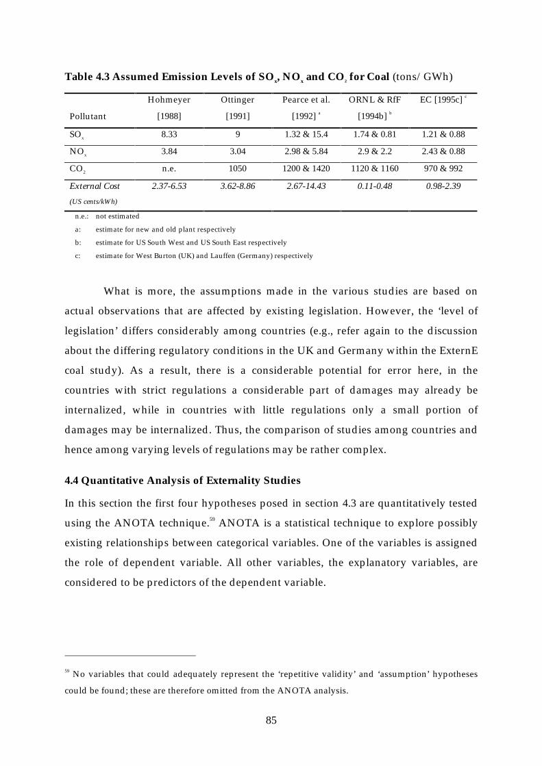
85
Table 4.3 Assumed Emission Levels of SOx, NOx and CO2 for Coal (tons/GWh)
Pollutant
Hohmeyer
[1988]
Ottinger
[1991]
Pearce et al.
[1992] a
ORNL & RfF
[1994b] b
EC [1995c] c
SOx 8.33 9 1.32 & 15.4 1.74 & 0.81 1.21 & 0.88
NOx 3.84 3.04 2.98 & 5.84 2.9 & 2.2 2.43 & 0.88
CO2 n.e. 1050 1200 & 1420 1120 & 1160 970 & 992
External Cost
(US cents/kWh)
2.37-6.53 3.62-8.86 2.67-14.43 0.11-0.48 0.98-2.39
n.e.: not estimated
a: estimate for new and old plant respectively
b: estimate for US South West and US South East respectively
c: estimate for West Burton (UK) and Lauffen (Germany) respectively
What is more, the assumptions made in the various studies are based on
actual observations that are affected by existing legislation. However, the ‘level of
legislation’ differs considerably among countries (e.g., refer again to the discussion
about the differing regulatory conditions in the UK and Germany within the ExternE
coal study). As a result, there is a considerable potential for error here, in the
countries with strict regulations a considerable part of damages may already be
internalized, while in countries with little regulations only a small portion of
damages may be internalized. Thus, the comparison of studies among countries and
hence among varying levels of regulations may be rather complex.
4.4 Quantitative Analysis of Externality Studies
In this section the first four hypotheses posed in section 4.3 are quantitatively tested
using the ANOTA technique.59 ANOTA is a statistical technique to explore possibly
existing relationships between categorical variables. One of the variables is assigned
the role of dependent variable. All other variables, the explanatory variables, are
considered to be predictors of the dependent variable.
59 No variables that could adequately represent the ‘repetitive validity’ and ‘assumption’ hypotheses
could be found; these are therefore omitted from the ANOTA analysis.

86
4.4.1 The Choice of Model
The ANOTA technique has been chosen for the analysis in this section. Other
possible ways of quantitatively assessing externality studies do however exist. It
would, for example, be possible to apply normal linear regression or logit analysis to
the data that the studies provide.60 However, since there are no theoretical reasons to
employ statistical procedures that are more intricate, and since most explanatory
variables used are discrete, the ANOTA technique will be easy to utilize in a
quantitative analysis as the one carried out below. Especially advantageous is the fact
that one is able to use a discrete dependent variable when assessing policy relevance,
i.e., the ANOTA technique allows for differentiation between ‘high’ and ‘low’
externality values, something that is not possible in, for example, OLS.
4.4.2 The ANOTA Model61
ANOTA resembles linear regression analysis. The main difference is that the
dependent variable in linear regression analysis should be numerical, whereas in
ANOTA dependent as well as explanatory variables are categorical.62 The estimated
coefficients have the same general interpretation as regression coefficients. They
measure the effect of the categories of the explanatory variables on categories of the
dependent variable as deviations from the average. The coefficients are corrected for
possible effects of other variables and therefore present 'pure' effects, and can
60 An attempt to explain the size of external cost estimates was made by Larsson [2000] under my
supervision. The author applied OLS to a log-linear model with the ‘worst-case’ external cost
estimates for coal and oil from 42 studies as the dependent variable. The results indicate that (at a 10
percent significance level) the use of the abatement cost approach affect results in a positive way and
so does (at a 1 percent significance level) the number of externalities monetized in the respective
studies. 61 For more on the ANOTA model and estimator, see Bethlehem [1990] and Keller et al. [1985]. For an
application of ANOTA analysis on data from the American Housing Survey National file 1983, see
Dieleman et al. [1989]. 62 Note that modelling using ANOTA is on the linear scale (accepting the disadvantages this involves).
It is hence assumed that an additive model adequately represents the data. However, since we have
no theory to base the model on there is no reason to assume a non-linear relationship.

87
consequently be interpreted as partial regression coefficients, i.e., as the percentage
probability of getting a value higher or lower than the average.
More formally, the ANOTA model originates from the following linear (e.g.,
regression) equation:
Xby =)(E (4.1)
where y is a n-vector of dependent scores, X a nxp-matrix of predictor scores, b a p-
vector of regression coefficients, and E(y) the expected value of y. The model can be
generalized to a multivariate linear model:
XBY =)(E (4.2)
where Y is a nxq-matrix, and B a pxq-matrix of regression coefficients. X is assumed
to be representative of the scores of the m predictor variables (i.e., each row contains
exactly m+1 times the value 1, and p-m-1 times the value 0). Y is a matrix of scores on
a dependent variable only assuming the values 0 and 1, with each row containing
exactly one 1. Consequently each row of E(Y) is a vector of probabilities summing to
1.
In order to interpret equation (4.2), consider the scalar representation of an
arbitrary element in the k-th column of (4.2), then we have:
)(),...,,(1
021 iki
m
ikmk jbbjjjp Σ
=+= (4.3)
with bk0 standing for the constant in the model, i.e., the k-th element in the first row of
B, and with bki(ji) equal to the k-th element of B in the row corresponding to the ji-th
category of the predictor variable Xi. Hence, the model says that the cell probabilities
are equal to the sum of regression coefficients, which depend only on the bivariate
indices.

88
4.4.3 ANOTA Analysis of Externality Studies
Appendix 2 presents all studies and variables included in the ANOTA analysis. A
total of 107 studies that assess externalities from electricity production have been
incorporated into the analysis (see table 4.4). More studies that have assessed
externalities have been identified (e.g., see Appendix 1), but these could for various
reasons not be categorized in a way that made inclusion possible.63 The dependent
and independent variables in the model and their categorization are discussed
below.
Table 4.4: Statistical Overview of Studies Included in the ANOTA Analysis
Fuel Source No of Obs.
Min
US cents/kWh
Max
US cents/kWh
Median
US cents/kWh
Mean
US cents/kWh
Coal 28 0.31 (US) 58.04 (Be) 8.30 12.52
Oil 13 0.32 (US) 31.99 (Fr) 12.35 11.96
Gas 21 0.10 (UK) 8.97 (Dk) 6.15 4.49
Nuclear 14 0.01 (Fr & US) 64.45 (US) 0.82 10.09
Hydro 10 0.02 (US) 26.26 (No) 0.35 4.44
Wind 14 0.001 (US) 2.53 (De) 0.27 0.43
Solar 7 0.15 (UK) 1.11 (De) 0.76 0.68
Total: 107 -- -- -- --
Sources: Appendix 2.
Dependent variable
The dependent variable is the ‘worst case’ total external cost (TEC) estimate
produced by the various studies.64 All estimates have been converted into US cents
(1998 price level) and for categorization these are compared to projected costs of
63 The reasons to why some studies could not be included mostly relate to categorization problems. For
example, some studies only present externality estimates per ‘amount’ of pollutant (e.g., Desvousges
et al. [1995] and Smead et al. [1997]), while some only present estimates for groups of pollutants (e.g.,
‘fossil fuels’ in Hohmeyer’s [1988 & 1992] studies), and finally some studies could simply not be
located (e.g., BPA [various years]). 64 By ‘worst case’ estimate it is meant that if the study has presented a possible range of external cost
values only the worst possible outcome (the high value) is included here. This since it is this estimate
that will have most of an impact on policy.

89
generating electricity as calculated by IEA/NEA [1998] for new generating capacity
commercially available by the years 2005-2010. IEA/NEA has projected generation
costs for different types of new capacity in 19 countries.65 The estimated costs range
from a low of 2.48 US cents per kWh to a high of 5.64 US cents per kWh for coal and
between 2.33-7.91 US cents per kWh for new gas, the total range for ‘all’ fuels is 2.33-
9.42 US cents per kWh (see table 4.5). No estimate is available in the report for hydro
and solar based power, and only one for oil based production. However, based on
projections from the Swedish National Energy Administration [1998] the total
production costs for these types of new capacity are approximately as high as for the
other fuels.
Table 4.5: Total Projected Generation Costs for New Capacity (US cents/kWh)
New Coal New Gas Nuclear Othersa Total
Min 2.48 (US) 2.33 (US) 2.54 (China) 3.00 (US)b 2.33
Max 5.64 (Brazil) 7.91 (Japan) 5.75 (Japan) 9.42 (Denmark)c 9.42
Mean 4.04 3.98 3.31 5.24 3.97
Median 4.03 3.74 3.22 4.69 3.71
a: Other fuels include cost projections for wind, oil, biomass, combined heat and straw fired power.
b: Projection for biomass fueled power generation.
c: Projection for straw fired power.
Source: IEA/NEA [1998].
More specifically, the projections presented by the Swedish National Energy
Administration roughly correspond to costs amounting to 3.4-4.5 US cents per kWh
for new gas capacity, 3.9-4.5 US cents per kWh for new oil capacity, 3.8-4.5 US cents
per kWh for new coal capacity, 3-3.4 US cents per kWh for new wind capacity, and
3.1-4.6 US cents per kWh for new hydroelectric capacity. This indicates that
electricity produced using new renewable capacity will, on average, be at least as
expensive as power generated from the other fuels. Furthermore, the cost projections
presented by the Swedish National Energy Administration are all within the range of
those calculated by IEA/NEA [1998]. For oil specifically, considering the recent trend
of increasing oil prices and projections of oil becoming the marginal fuel from which
65 The IEA/NEA [1998] cost projection are taken from table 15 [pp. 66-67] and have been derived using
‘generic assumptions’ and a five percent discount rate.

90
to produce electricity (see for example the discussion in Paffenbarger [1997]) the use
of IEA/NEA cost predictions as a minimum proxy for the costs of new oil capacity
seems reasonable. The average cost of new capacity has, based on the IEA/NEA
projections, been estimated at 3.97 US cents per kWh. This average value for the
‘internal costs’ of new capacity will be used as a basis for the categorization of the
external costs for the different fuels.
As a comparison the TEC estimates for coal range between 0.31 and 58.04 US
cents per kWh with an average external cost of 11.35 US cents per kWh, for oil the
same range is 0.32-31.99 US cents per kWh with an average of 12.33 US cents per
kWh, and for natural gas 0.10-9.44 US cents per kWh, and average of 4.60 US cents
per kWh.
The categorization of the TEC estimates is based on their relative impact on
production costs (and thus indirectly on price), i.e., as follows:
I. Low: studies with a ‘moderate’ impact, i.e., where external costs are less than
or equal to projected average internal cost of producing electricity. (��3.97 US
cents/kWh) (62 studies)
II. High: studies with a ‘big’ impact, i.e., where external costs amount to more
than 100 percent of projected average internal cost. (> 3.97 US cents/kWh) (45
studies)
Categorizing the dependent variable in some other way is certainly possible,
especially since there is no theoretical basis on which the categorization can rely. The
present categorization is however chosen so as to reflect the included studies in a
reasonable way while still being transparent enough to distinguish between
estimates that will have a ‘big’ impact on the costs of power plants (and indirectly on
prices) and those that will have a ‘moderate’ impact.
Explanatory Variables
The first explanatory variable is the methodological approach chosen by the individual
studies. There are, as we have seen, basically three approaches that can be used (see
chapter 2 for a more thorough discussion of these). The categorization of the studies
is hence:

91
I. AC: Abatement Cost. (12 studies)
II. TD: Top-Down Damage Cost. (17 studies)
III. BU: Bottom-Up Damage Cost. (78 studies)
For the bottom-up studies a more transparent categorization that reflect the
monetization of impacts more correctly would probably be preferable, this since the
approach relies on different techniques to actually derive monetary values while the
other two approaches ‘directly’ give monetary estimates of the external costs and
benefits involved.66 Theoretically, the choice between these approaches should not
affect the resulting external cost estimates, i.e., the choice of methodology should not
matter! The possibility of getting a low (or high) externality value should hence be
unrelated to the methodological approach, this since the approaches basically
measure the same thing, i.e., damage done. However, based on the discussion of the
abatement cost in chapters 2 and 3, there might be some justification for assuming
that the choice of this specific approach might, on average, produce higher estimates,
or in other words, that the possibility of getting a low externality value will decrease
(i.e., negative sign), ceteris paribus, if a study chooses the abatement cost approach.
Following the same reasoning, the use of the bottom-up damage cost approach will
increase the possibility of getting a low value (i.e., positive sign).
The other explanatory variables are included to capture other possible effects
that may affect the size of the external cost estimate. The first of these, fuel type is
included to capture any effects that the type of fuel might have on estimated costs.
The variable is thus incorporated into the analysis since it (implicitly) reflects the
differences in externalities among the different fuels. The categorization of the
variable is given by:
I. COAL: studies of coal based electricity production. (29 studies)
II. OIL: studies of oil based electricity production. (13 studies)
III. GAS: studies of natural gas based electricity production. (20 studies)
IV. NUCLEAR: studies of nuclear based electricity production. (14 studies)
66 The classification of the ‘method’-variable in order to take this issue into consideration would
however become extremely complicated since the monetization of impacts in the bottom-up studies
have relied on a considerable number of different techniques.

92
V. HYDRO: studies of hydroelectric production. (10 studies)
VI. WIND: studies of wind based electricity production. (14 studies)
VII. SOLAR: studies of solar based electricity production. (7 studies)
Generally it is expected that the use of the more environmentally benign fuels (e.g.,
wind and solar) as a basis for power production will negatively affect estimates (i.e.,
increasing probability of low estimate), while the allegedly ‘bad’ fuels (e.g., coal and
oil) are expected to positively affect external cost estimates (i.e., decreasing
possibility). Doing this allows us to capture what is of relevance for policy-makers in
the fuel choice issue, i.e., whether some fuels are, ceteris paribus, better or worse than
others.
The third explanatory variable pertains to whether the individual studies
have addressed the full fuel cycle, i.e., fuel stages other than generation (e.g.,
extraction and transport). This variable is included to capture the ‘thoroughness’ of
each study. It is expected that the studies that, everything else held constant, have
addressed stages other than generation will give a higher external cost estimate.
Thus, including more of the fuel cycle is expected to positively affect externality
estimates, i.e., lower probability of getting a low value (negative sign). The
categorization is then as follows:
I. YES: studies that have assessed other stages than generation. (63 studies)
II. NO: studies that only assessed generation impacts. (44 studies)
The fourth explanatory variable is income. The measure used for
categorization is GDP per capita for 1996 expressed in (PPP corrected) USD to make
comparison possible. The measure is supposed to capture how income variations as
well as regional variations affect externality estimates. That is, to (in some way) test
the hypothesis of country-specificity. It is expected that the higher the income the
higher the willingness to pay for avoiding damage, thus, higher GDP per capita
should positively affect external costs (and hence lead to lower possibility of getting
a low value).67 However, there are only two ‘developing countries’ among the
studies, India and South Africa. This makes the normal categorization (developed or
developing) non-transparent. There would then be two countries in the ‘poor’
67 In some sense, this variable is supposed to capture the environment being a luxury good.
93
category and 26 in the rich category. There are still plenty of differences among the
countries in the developed world that would not be captured by this categorization,
an example being the US with a GDP per capita of 28023 USD and Portugal with a
GDP per capita of 13535 USD both qualifying for the developed group. A more
transparent categorization does (to the authors knowledge) not exist. After
examining the GDP per capita values of the various countries included in the
analysis it was concluded that the ‘significant’ gap between Ireland’s GDP per capita
(18634 USD) and Portugal’s (13535 USD) would be used for categorizing the studies.
The income variable is thus categorized as follows:
I. LOW: studies in countries with a GDP per capita less than 18684 USD. (13
studies)
II. HIGH: studies in countries with a GDP per capita greater than or equal to 18684
USD. (94 studies)
The final explanatory variable included is population density (i.e., people per
square kilometer) in each of the countries considered. This variable is also included
to verify the validity of the country-specificity supposition. A high population
density is expected to positively affect external costs (i.e., decreasing probability of a
low value). This since more people will be affected in a densely populated area than
in a sparsely populated area. Hence, the total willingness to pay to avoid a negative
externality in an area with many people will, ceteris paribus, be higher than in an area
with less people. No obvious way of categorizing this variable could be found so the
categorization chosen is based on the median value (102 people per square
kilometer). Hence, the categorization of the variable is as follows:
I. LOW: studies in countries with less than 102 people per square kilometer. (47
studies)
II. HIGH: studies in countries with more than 102 people per square kilometer.
(60 studies)
Some caveats of the model must be noted before we go on with the analysis.
The model derived above is probably not ‘optimal’; two of the hypotheses discussed
in section 4.3 (i.e., ‘repetitive validity’ and ‘assumptions’) have been omitted from the
model, and there may be other important explanatory variables that have been left
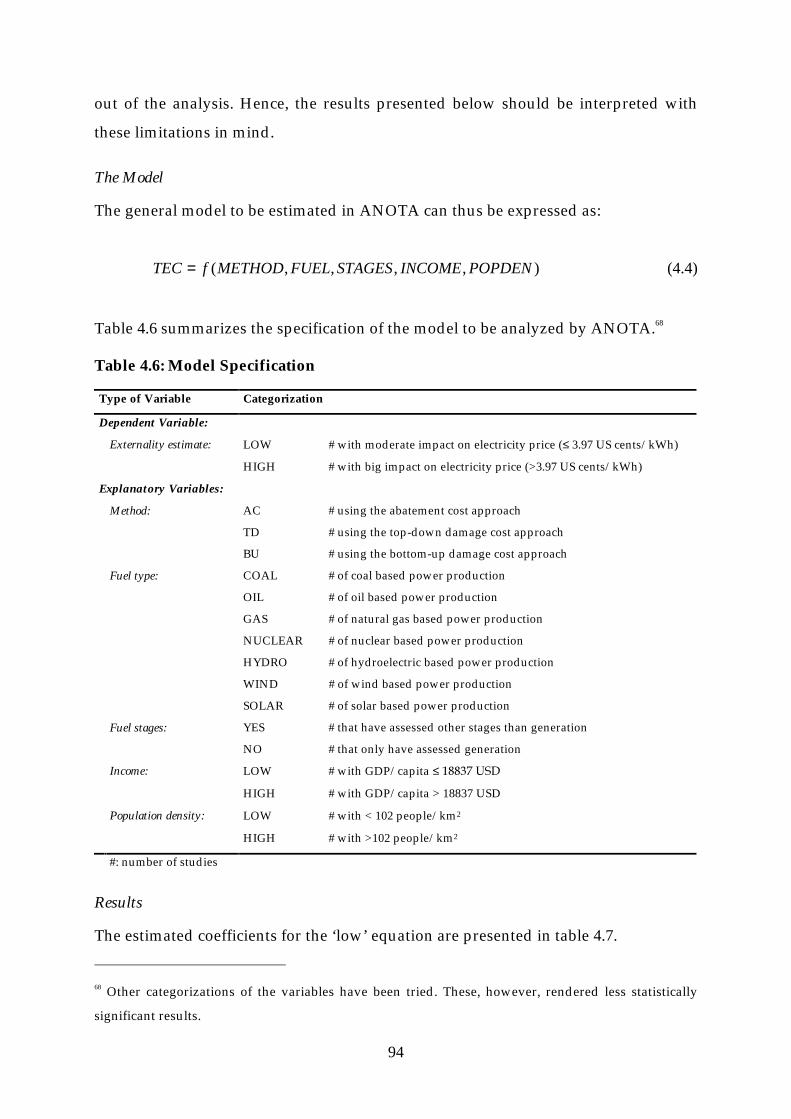
94
out of the analysis. Hence, the results presented below should be interpreted with
these limitations in mind.
The Model
The general model to be estimated in ANOTA can thus be expressed as:
),,,,( POPDENINCOMESTAGESFUELMETHODfTEC = (4.4)
Table 4.6 summarizes the specification of the model to be analyzed by ANOTA.68
Table 4.6: Model Specification
Type of Variable Categorization
Dependent Variable:
Externality estimate: LOW # with moderate impact on electricity price (� 3.97 US cents/kWh)
HIGH # with big impact on electricity price (>3.97 US cents/kWh)
Explanatory Variables:
Method: AC # using the abatement cost approach
TD # using the top-down damage cost approach
BU # using the bottom-up damage cost approach
Fuel type: COAL # of coal based power production
OIL # of oil based power production
GAS # of natural gas based power production
NUCLEAR # of nuclear based power production
HYDRO # of hydroelectric based power production
WIND # of wind based power production
SOLAR # of solar based power production
Fuel stages: YES # that have assessed other stages than generation
NO # that only have assessed generation
Income: LOW # with GDP/capita ����������
HIGH # with GDP/capita > 18837 USD
Population density: LOW # with < 102 people/km2
HIGH # with >102 people/km2
#: number of studies
Results
The estimated coefficients for the ‘low’ equation are presented in table 4.7.
68 Other categorizations of the variables have been tried. These, however, rendered less statistically
significant results.
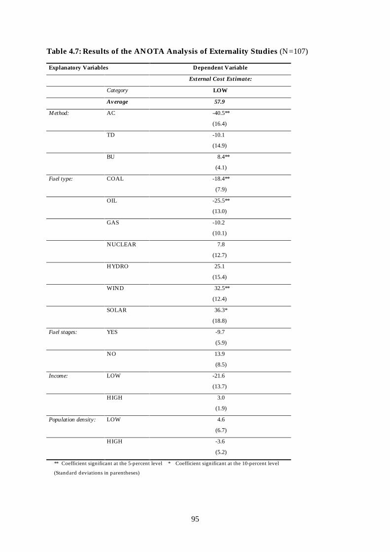
95
Table 4.7: Results of the ANOTA Analysis of Externality Studies (N=107)
Explanatory Variables Dependent Variable
External Cost Estimate:
Category LOW
Average 57.9
Method: AC -40.5**
(16.4)
TD -10.1
(14.9)
BU 8.4**
(4.1)
Fuel type: COAL -18.4**
(7.9)
OIL -25.5**
(13.0)
GAS -10.2
(10.1)
NUCLEAR 7.8
(12.7)
HYDRO 25.1
(15.4)
WIND 32.5**
(12.4)
SOLAR 36.3*
(18.8)
Fuel stages: YES -9.7
(5.9)
NO 13.9
(8.5)
Income: LOW -21.6
(13.7)
HIGH 3.0
(1.9)
Population density: LOW 4.6
(6.7)
HIGH -3.6
(5.2)
** Coefficient significant at the 5-percent level * Coefficient significant at the 10-percent level
(Standard deviations in parentheses)

96
The ANOTA-program also presents coefficients for the ‘high’ equation
(average 42.1, i.e., the percent of observations assigned the ‘high’ classification).
However, when the dependent variable only has two categories exactly the same
coefficients (only with opposite signs, i.e., the rows sum to zero) and standard
deviations are presented. The ‘high’ equation is therefore not presented above.
The results of the ANOTA analysis reveal that several of the explanatory
variables significantly affect the size of externality estimates in the considered
studies. First, considering the method variables, it can be established that the use of
the abatement cost approach decreases the possibility of getting a low external cost
estimate (a result that is statistically significant at the 5-percent level). I.e., as was
expected, and not in line with economic theory, the preceding analysis shows that on
average, the use of abatement costing will produce higher externality estimates. The
sign on the top-down variable also indicates that, as expected, the use of the top-down
approach tends to lower the possibility of getting a low external cost estimate (this
result is however not statistically significant). The results further show that the use of
the bottom-up approach significantly affects externality estimates. As a priori
expected, the probability of getting a low value is, ceteris paribus, higher when
bottom-up approach is used. Hence, overall it can be established that the choice of
method matters and that this provides one explanation to the divergence of
externality costing results. The interpretation of the coefficients is as follows; the use
of the abatement cost approach will lower the probability of getting a value lower
than the average by 40.5 percentage points, i.e., the probability of getting a low value
when using the abatement cost approach is 17.4 percent, while given that the bottom-
up approach is used in a study, the probability of getting a low value is, hence, 66.3
percent.
The coefficients for the fuel type variables show that there are differences
between fuels, i.e., as expected, that some of the fuels (especially the coal and oil)
have more adverse impacts than do the renewables. For gas, nuclear and hydro no
significance could be established, however the signs indicate that the probability of
getting a low external cost estimate decreases when gas is the fuel under study and
that it increases when nuclear and hydro are the assessed fuels. In the ANOTA
analysis it is, in contrast with the earlier analysis (see, for example, the discussion

97
concerning figure 4.1), thus possible, holding everything else constant, to establish
that certain fuels tend to give rise to higher environmental damages (and hence
produce higher externality estimates), a result that is of relevance for policy-makers
when they make decisions about future generation.
For the explanatory variable, fuel stages, no significance could be established
at the five percent level. The signs are, however, as expected, thus suggesting that
assessing other stages in the fuel cycle than generation will on average produce
higher externality estimates and lending some support to the thoroughness
hypothesis.
Neither could any statistical significance be established for the two ‘site- and
country-specificity’ variables income and population density. Furthermore, the signs of
the income variable are not in line with what could be expected. For population
density, the signs are however in agreement with the a priori expectations (but far
from significant), i.e., indicating that the higher the population density, the lower the
probability of getting a ‘low’ externality estimate. The lack of significance indicates
that the site- and country-specificity argument, that has been put forward as the
main explanation to the disparity of results, may not be valid. Note however that
these measures can be considered rather ‘coarse’, i.e., they may not fully account for
the variation due to site- and country-specificity.
The ANOTA program also tests for overall significance using confidence
intervals, i.e., it tests whether the full predicted equations are significantly different
from zero at the 5-percent level (e.g., compare with the F-test of overall significance
in OLS analysis). The confidence intervals reveal (see table 4.8) that the estimated
equations are not significantly different from zero (and one) at the 5-percent level
(i.e., the ranges includes zero and one for both equations). Thus, the estimated model
as a whole cannot be considered significant, suggesting, as can be expected, model
misspecification, i.e., that relevant variables may have been omitted, and therefore
some caution should be used in the interpretation of the model.69
69 This is, at least in part, as expected. As discussed in section 4.3 above, there may be other
explanations to the divergence of externality estimates (e.g., differences in assumptions) that are not
included in the ANOTA analysis.

98
Table 4.8: 95-Percent Confidence Intervals for the Estimated Equations
Estimated Equation Min Max
LOW -42.9 124.2
HIGH -24.2 142.9
4.5 Concluding Remarks
The purpose of this chapter has been to establish if there are any systematical
explanations to the discrepancy of results among the different studies. This problem
was addressed by the formulation of hypothetical explanations; these hypotheses
were then examined using both verbal and graphical analysis (section 4.3) and
through quantitative analysis utilizing the ANOTA technique (section 4.4).
To sum up, the results of the analysis indicate that the choice of model tends
to affect the results. In particular the use of the abatement cost approach will
positively affect external cost estimates, while the bottom-up damage cost approach
will on average give lower external cost estimates than the other approaches.
Furthermore, there also seems to be statistically significant differences among the
different types of fuels. For example, the fossil fuels (especially coal and oil) seem to,
on average, cause more adverse impacts than do the renewables, wind and solar, a
result of importance for future fuel choices. What is more, the results derived in this
chapter also suggest that the most commonly accepted explanation to the
discrepancies in externality estimates among studies, namely country and site-
specificity, may be invalid, or ‘irrelevant’. It is, however, in general hard to compare
the studies since they differ with respect to methodological choice and scope,
something that limits their relevance for policy. The analysis here is limited to
establishing if there are any systematical differences among electricity externality
studies, i.e., as to why the numbers differ. It should, hence, be noted that the analysis
carried out here do not (neither does it attempt to) answer the question of what is the
true external cost (if one exists).

99
Chapter 5
A SUMMARY OF THE MAIN FINDINGS
The purposes of this thesis were; first, to critically survey existing electricity
externality studies (especially in the context of comparability and policy relevance),
and second, to analyze if there are any systematical explanations to the disparity of
results among studies. The approach chosen to address these issues was to carefully
examine the existing studies. This was done in two steps, first a sample of influential
previous studies were qualitatively reviewed and scrutinized, and second, a majority
of all studies were quantitatively assessed utilizing the statistical technique ANOTA.
The first part of the qualitative analysis, carried out in chapter 3, indicates
that the following three main conclusions may be drawn. First, there exist theoretical
reasons to suspect that the abatement cost approach produces higher estimates in
general, thus implying that there are methodological reasons to the discrepancies in
the results of the various studies. Second, there are several problems in the
application of the various methodologies that may help explain the disparity of
estimated damages. Furthermore, some of the studies have included costs (and
benefits) into the calculation that cannot be considered to comprise externalities. This
is due to the differences in scope; these studies are attempting to assess the ‘full’ cost
of the fuel cycles under consideration (i.e., something above pure externality cost
appraisal). Third, the thoroughness of approach differs considerably among the
studies, both when it comes to the specific impacts that the studies consider, and
pertaining to the stages in the fuel cycle that are assessed.
In chapter 4, building on the analysis in chapter 3, five hypotheses was
developed as possible explanations to the disparity of externality estimates. First,
(site and country specificity) the size of impacts will depend on the specific location of
the power plant. Second, (convergent validity) different quantification and valuation
methods tend to produce different results. Third, (repetitive validity) the application of

100
quantification and valuation methodologies in similar contexts may produce
different results. Fourth, (thoroughness) one study may differ from another by simply
taking a more comprehensive approach to the issue of externality appraisal. Five,
(assumptions) the basic assumptions made in the development of damage estimates in
a study may also affect the size of estimates.
The qualitative part of chapter 4 addressed each of these hypothetical
explanations in turn. The analysis indicated that little support could be established
for the first (site-and country-specificity) hypothesis. One reason to this might, for
example, be that there in some cases is no actual site under study. With respect to the
second hypothesis (convergent validity), the analysis provided ambiguous insights;
no clear tendencies could be discerned. Furthermore, based on graphical analysis, the
third hypothesis (repetitive validity) seems to be a reasonable explanation to the
disparity of results (i.e., that externality estimates do not seem to converge). Also, it
could not be established that one of the methodological approaches on average tends
to produce more similar results than others. Examining the fourth hypothesis
(thoroughness) also provides somewhat vague insights. For example, including more
impacts into the analysis does not seem to affect totals. On the other hand, it is
apparent that omitting certain impacts (such as CO2 damages) seems to significantly
affect the size of externality estimates. Based on the analysis, the assumptions
(number five) used in each study also seem to affect estimates.
The quantitative analysis carried out in chapter 4 demonstrates that the
choice of methodological approach affects the results, e.g., that the second
hypothetical explanation (convergent validity) may be valid. Furthermore, there also
seems to be statistically significant differences among the different types of fuels, a
result indicating that the externality studies are of some relevance for the specific
issue of fuel choice. No significance could, however, be established for the
thoroughness of approach taken in each study. What is more, the results derived in
chapter 4 also suggest that the most commonly accepted explanation to the
discrepancies in externality estimates among studies, namely site and country-
specificity (hypothesis one), may be invalid.
To sum up, do the numbers make sense? To some extent they do. There are
several reasonable (systematical) explanations to the discrepancy of results. The

101
analysis has shed some light on the issue. For example, it has been shown that the
choice of methodological approach tends to affect the estimates, and after having
taken account of this and similar impacts, the external cost ranking by fuel becomes
easier. Thus, in contrast to what a superficial observation of figure 4.1 might lead one
to conclude, the possibility of ranking different fuel sources using the results in these
studies, might not be a hopeless task. The analysis carried out is, however, not
sufficient to explain all of the variability in externality estimates. When it comes to
the issue of clarifying the relevance for policy it must be concluded that it may be
limited (especially for the studies relying on the abatement cost approach). Thus, the
possibility of making rational decisions based on the results of previous studies is
questionable.
This is reflected by the fact that the studies are hard to compare directly, this
because they differ with respect to:
• scope (e.g., some studies want to achieve more than simply evaluate external
cost and benefits),
• methodologies used (which tend both to produce different empirical results
and even differ in terms of theoretical basis),
• basic assumptions (e.g., emission factors),
• how existing regulations are dealt with, and
• thoroughness.
However, even if the studies carried out this far may be of limited relevance
to policy makers, the fact that they have been carried out means that new methods
and approaches to the issue of externality appraisal has had to be developed (forced
learning). Consequently, past research efforts may have increased the possibilities of
deriving more robust externality estimates in the future. Thus, future studies that can
avoid the problems encountered in the studies carried out during the 1980s and
1990s may be of more relevance to policy. For this to come true, however, analysts
and policy makers must come to some kind of consensus on how to deal with the
five issues just raised above. For example, guidelines must be established for what
scope externality studies should have, which methodological approach to employ,
and how thorough researchers should be in their assessment, etc.

102
In doing this, one has to raise the issue of how far one should go in the search
for the ‘true’ external cost. Where should one draw the line between political values
on the one hand and economic analysis on the other? This question cannot be
answered by pursuing further externality studies; it has to be resolved within the
realms of public discourse. It is probably fair to conclude that before this is done
externality studies, as those surveyed in this thesis, will continue to provide limited
guidance to policy makers.
103
REFERENCES
Adamowicz, W.; Boxall, P.; Williams, M. & Louviere, J. [1998]. Stated Preference
Approaches for Measuring Passive Use Values: Choice Experiments and
Contingent Valuation. American Journal of Agricultural Economics, 80 (February),
pp. 64-75.
Arrow, K.; Solow, R.; Portney, P.R.; Leamer, E.E.; Radner; R. & Schuman, H. [1993].
Report of the NOAA Panel on Contingent Valuation. Federal Register, 58 (10), pp.
4601-4614.
Ayres, R.U. & Kneese, A.V. [1969]. Production, Consumption and Externalities.
American Economic Review, 59 (3), pp. 282-287.
Baumol, W.J. & Oates, W.E. [1988]. The Theory of Environmental Policy (2nd Edition).
Cambridge: Cambridge University Press.
Bernow, S. & Marron, D. [1990]. Valuation of Environmental Externalities for Energy
Planning and Operations, May 1990 Update (Tellus Institute Report 90-SB01). Boston,
MA: Tellus Institute.
Bernow, S.; Biewald, B. & Marron, D. [1991]. Full-Cost Dispatch: Incorporating
Environmental Externalities in Electric System Operation. The Electricity Journal
(March), pp. 20-33.
Bernow, S.; Biewald, R. & Wolcott, D. [1993]. Modelling Fuel Cycle and Site-
Dependent Environmental Impacts in Electric Resource Planning. (in Expert
Workshop on Life-Cycle Analysis of Energy Systems – Proceedings, Paris, France, 21-22
May 1992). Paris: OECD/IEA.
Bethlehem, J.G. [1990]. The Program ANOTA 5.0 for the Analysis of Tables. Voorburg:
Netherlands Central Bureau of Statistics.
Bhattacharyya, S.C. [1997]. An Estimation of Environmental Costs of Coal-Based
Thermal Power Generation in India. International Journal of Energy Resources, 21,
pp. 289-298.
Binning, C.; Carter, M; Mackie, K.; Matthews, N.; McGlynn, G.; McVay, P.; Palmer,
D.; Scoccimarro, M. & Wilks, L. [1996]. Techniques to Value Environmental Resources:

104
An Introductory Handbook. Canberra: Department of the Environment, Sports and
Territories.
Bohi, D.R. [1993]. A Perspective on Energy Security and Other Nonenvironmental
Externalities in Electricity Generation (Discussion Paper ENR 93-23). Washington,
DC: Resources for the Future.
Bonneville Power Administration [BPA]. [1983]. Final Report: Economic Analysis of the
Environmental Effects of the Coal-Fired Electric Generator at Boardman, Oregon.
(Report commissioned by the Bonneville Power Administration, prepared by
ECO Northwest et. al., Dec. 23, 1983).
Bonneville Power Administration [BPA]. [1984a]. Environmental Costs and Benefits
Case Study: Nuclear Power Plant, Quantification and Economic Valuation of Selected
Environmental Impacts/Effects. (Report prepared for the Bonneville Power
Administration, prepared by Nero and Associates, Inc, February, 1984).
Bonneville Power Administration [BPA]. [1984b]. Economic Analysis of the
Environmental Effects of a Combustion-Turbine at Frederickson Industrial Park, Pierce
County, Washington. (Report commissioned by the Bonneville Power
Administration, prepared by ECO Northwest et al., March, 1984).
Bonneville Power Administration [BPA]. [1984c]. Final Report: Methods for Valuation of
Environmental Costs and Benefits of Hydroelectric Facilities. A Case Study of the Sultan
River Project. (Report commissioned by the Bonneville Power Adminstration,
prepared by Biosystems Analysis, Inc. June, 1984).
Bonneville Power Administration [BPA]. [1986]. Estimating Environmental Costs and
Benefits for Five Generating Resources. (Report commissioned by the Bonneville
Power Administration, prepared by ECO Northwest et al., March, 1986).
Bonneville Power Administration [BPA]. [1987]. Generic Coal Study: Quantification and
Valuation of Environmental Impacts. (Report commissioned by the Bonneville
Power Administration, prepared by ECO Northwest et al., January, 1987).
Brännlund, R. & Kriström, B. [1998]. Miljöekonomi (in Swedish). Lund:
Studentlitteratur.
Carlifornia Energy Commission (CEC). [1993]. 1992 Electricity Report (P104-92-001).
Sacramento, CA: CEC.

105
Carlsen, A.J.; Strand, J. & Wenstøp, F. [1991]. Beregening av implisite miljøkostnader
ved utbygging av vannkraft: En analyse av prosjekten i Samlet plan for vassdrag.
Sosialøkonomen, (10), pp. 26-30.
Carlsen, A.J.; Strand, J. & Wenstøp, F. [1992]. Implicit Environmental Costs in
Hydroelectric Development: An Analysis of the Norwegian Master Plan for Water
Resources (Memorandum No. 1). Oslo: Department of Economics, University of
Oslo.
Carlsen, A.J.; Strand, J. & Wenstøp, F. [1993]. Implicit Environmental Costs in
Hydroelectric Development: An Analysis of the Norwegian Master Plan for Water
Resources. Journal of Environmental Economics and Management, 23 (3), pp. 201-211.
Chernick, P. & Caverhill, E. [1989]. The Valuation of Externalities from Energy
Production, Delivery, and Use Fall, 1989 Update. (A Report to the Boston Gas
Company). Boston, MA: PLC, Inc.
Chernick, P. & Caverhill, E. [1990]. Report to the Boston Gas Company on Including
Externalities (89-239). Boston, MA: Boston Gas Company.
Clarke, L. B. [1996]. Externalities and Coal-fired Power Generation (IEAPER/29).
London: IEA Coal Research.
Cline, W. [1992]. The Economics of Global Warming. Washington, DC: Institute for
International Economics.
Coase, R.H. [1960]. The Problem of Social Cost. Journal of Law and Economics, 3
(October), pp. 1-44.
Connolly, D. & Rooney, S. [1998]. The National Implementation in Ireland of the ExternE
Accounting Framework. Dublin: Environmental Institute, University College
Dublin.
Crapanzano, G.; Del Furia, L.; Pavan, M.; Ascari, S.; Fontana, M.; Lorenzoni, A. &
Maugliani, F. [1998]. ExternE National Implementation, Italy. Milano: Fondazione
Eni Enrico Mattei (FEEM).
De Nocker, L.; Torfs, R. & Wouters, G. [1998]. ExternE Implementation in Belgium. Mol,
Belgium: Flemish Institute for Technological Research (VITO).
Desvousges, W.H.; Johnson, F.R.; Banzhaf, H.S.; Russel, R.R.; Fries, E.E.; Dietz, K.J.;
Helms, S.C.; Keen, D.; Snyder, J.; Balantine, H.; Sadeghi, V. & Martin, S.A. [1995].

106
Assessing Environmental Externality Costs for Electricity Generation (Final Report,
May 1995). Durham, NC: Triangle Economic Research.
Desvousges, W. H.; Johnson, F. R. & Banzhaf, H. S. [1998]. Environmental Policy
Analysis with Limited Information: Principles and Applications of the Transfer Method.
Cheltenham: Edward Elgar Publishing.
Diakoulaki, D.; Mirasgentis, S.; Koukios, E.; Diamantidis, N. & Stamos, C. [1997].
External Costs of Electricity Generation in Greece. Athens: Laboratory of Industrial
and Energy Economics, National Technical University of Athens.
Dieleman, F.M.; Clark, W.A.V.; & Deurloo, M.C. [1989]. A Comparative View of
Housing Choices in Controlled and Uncontrolled Housing Markets. Urban Studies,
(26), pp. 457-468.
Dorland, C.; Jansen, H.M.A; Tol, R.S.J. & Dodd, D. [1997]. ExternE National
Implementation - Externalities of electricity production in the Netherlands. Amsterdam:
Institute for Environmental Studies E97/17, Vrije Universiteit.
Energy Information Administration (EIA), US Department of Energy. [1995].
Electricity Generation and Environmental Externalities: Case Studies (DOE/EIA-0598).
Washington, DC: US Department of Energy.
European Commission [EC]. [1995a]. ExternE: Externalities of Energy (Vol. 1:
Summary) Luxembourg: Office for Official Publications of the European
Communities.
European Commission [EC]. [1995b]. ExternE: Externalities of Energy (Vol. 2:
Methodology). Luxembourg: Office for Official Publications of the European
Communities.
European Commission [EC]. [1995c]. ExternE: Externalities of Energy (Vol. 3: Coal &
Lignite). Luxembourg: Office for Official Publications of the European
Communities.
European Commission [EC]. [1995d]. ExternE: Externalities of Energy (Vol. 4: Oil &
Gas). Luxembourg: Office for Official Publications of the European Communities.
European Commission [EC]. [1995e]. ExternE: Externalities of Energy (Vol. 5: Nuclear).
Luxembourg: Office for Official Publications of the European Communities.
107
European Commission [EC]. [1995f]. ExternE: Externalities of Energy (Vol. 6: Wind &
Hydro). Luxembourg: Office for Official Publications of the European
Communities.
Faaij, A.; Meuleman, B.; Turkenburg, W.; van Wijk, A.; Bauen, A.; Rosillo-Calle, F. &
Hall, D. [1998]. Externalities of Biomass Based Electriciy Production Compared
with Power Generation from Coal in the Netherlands. Biomass and Energy, 14 (2),
pp. 125-147.
Fankhauser, S. [1993]. Global Warming Damage Costs - Some Monetary Estimates
(CSERGE Working Paper GEC 92-29). University College London and University
of East Anglia.
Freeman, A.M., III. [1993]. The Measurement of Environmental and Resource Values:
Theory and Methods. Washington, DC: Resources for the Future.
Freeman, A. M., III. [1996]. Estimating the Environmental Costs of Electricity: An
Overview and Review of the Issues. Resource and Energy Economics, 18 (4), pp. 347-
362.
Friedrich, R. & Kallenbach, U. [1991]. External Costs of Electricity Generation (in
External Environmental Costs of Electric Power: Analysis and Internalization,
Hohmeyer, O. & Ottinger, R.L. (Eds.)). Berlin: Springer-Verlag.
Friedrich, R. & Voss, A. [1993]. External Costs of Electricity Generation. Energy Policy,
(February), pp. 114-122.
Hanemann, W.M. [1991]. Willingness To Pay and Willingness To Accept: How Much
Can They Differ? American Economic Review, 81 (3), pp 635-647.
Hervik, A.; Strøm, S. & Aaheim, A. [1985]. Implisitte kostnadsberegninger for Samlet
Plan. Sosialøkonomen, (3), pp. 3-6.
Hervik, A.; Risnes, M. & Strand, J. [1986]. Betalningsvillighet for vern av vassdrag i
forbindelse med Samlet Plan. Sosialøkonomen, (1), pp. 2-7.
Hohmeyer, O. [1988]. Social Costs of Energy Consumption. Berlin: Springer-Verlag.
Hohmeyer, O. [1992]. The Social Costs of Electricity – Renewables Versus Fossil and
Nuclear Energy. International Journal of Solar Energy, 11, pp. 231-250.
Hohmeyer, O. & Gärtner, M. [1992]. The Costs of Climate Change. Fraunhofer Institute
fur Systemtechnik und Innovationsforschung.

108
Holland, M.R.; Berry, J.E.; Watkiss, P.; Boyd, R. & Stephenson, W. [1998]. Power
Generation and the Environment - A UK Perspective. Culham: AEA Technology plc.
van Horen, C. [1996]. Counting the Social Costs: Electricity and Externalities in South
Africa. Cape Town: Élan Press & UCT Press.
International Energy Agency & Nuclear Energy Agency (IEA/NEA) [1998]. Projected
Costs of Generating Electricity. Paris: OECD Publications.
Izmir, G. [1993]. Valuation of Environmental Impacts (Technical Paper). Sydney:
Environmental Protection Agency of New South Wales.
Johansson, P-O. [1993]. Cost-Benefit Analysis of Environmental Change. Cambridge:
Cambridge University Press.
Joskow, P.L. [1992]. Weighing Environmental Externalities: Let’s Do It Right.
Electricity Journal, (May), pp. 53-67.
Kahnemann, D.; Knetsch, J. & Thaler, R. [1990]. Experimental Tests of the
Endowment Effect and the Coase Theorem. Journal of Political Economy, 98 (6), pp.
1325-1348.
Keller, W.J.; Verbeek, A. & Bethlehem, J. [1985]. ANOTA: Analysis of Tables. Voorburg:
Netherlands Central Bureau of Statistics.
Koomey, J. & Krause, F. [1997]. Introduction to Environmental Externality Costs (in
the CRC Handbook on Energy Efficiency). Boca Raton, FL: CRC Press, Inc.
Krewitt, W.; Mayerhofer, P.; Friedrich, R.; Trukenmüller, A.; Heck, T.; Greßmann, A.;
Raptis, F.; Kaspar, F.; Sachau, J.; Rennings, K.; Diekmann, J. & Praetorius, B.
[1998]. ExternE - Externalities of Energy. National Implementation in Germany.
Stuttgart: IER, University of Stuttgart.
Larsson, J. [2000]. Does the Methodological Choice Influence the Results of Externality
Studies? Master Thesis (2000:039), Luleå University of Technology.
Lashof, D.A. & Ahuja, D.P. [1990]. Relative Contributions of Greenhouse Gas
Emissions to Global Warming. Nature, 344 (April), pp. 524-531.
Lee, R. [1996]. The External Costs of Electricity Generation: An “Insider’s”
Perspective on the Lessons from the US Experience. Energy Studies Review, 8 (2),
pp. 177-186.
Lee, R. [1997]. Externalities Studies: Why are the Numbers Different? (in Social Costs
and Sustainability: Valuation and Implementation in the Energy and Transport Sector

109
(Conference Proceedings), Hohmeyer, O.; Ottinger, R.L. & Rennings, K. (Eds.)).
Berlin: Springer-Verlag.
Lesser, J.A.; Dodds, D.E. & Zerbe, R.O. Jr. [1997]. Environmental Economics and Policy.
Cambridge, MA: Addison-Wesley.
Linares, P.; Aróstegui, M.; Leal, J.; Lechón, Y.; Sáez, R.M.; Varela, M.; Alarcón, A.;
Salat, S.; Sumarroca, N.; Montes, J.; Muñoz, L. & Ramos, A. [1998]. ExternE
National Implementation. Spain. Madrid: CIEMAT.
Maddison, D. [1999]. The Plausibility of the ExternE Estimates of the External Effects of
Electricity Production (CSERGE Working Paper GEC 99-04). University College
London and University of East Anglia.
Martin, P-E. [1995]. The External Costs of Electricity Generation: Lessons from the US
Experience. Energy Studies Review, 7 (3), pp. 232-246.
Martins, A.; Fernandes, M.; Rodrigues, V. & Ramos, T. [1998]. Implementation in
Portugal of the ExternE accounting framework. Lisbon: Centro de Estudos em
Economia da Energia, dos Transportes e do Ambiente (CEEETA).
Mishan, E.J. [1969]. The Relationship Between Joint Products, Collective Goods and
External Effects. Journal of Political Economy, 77 (3), pp. 329-348.
Mitchell, R.C. & Carson, R.T. [1989]. Using Surveys to Value Public Goods: the
Contingent Valuation Method. Washington, DC: Resources for the Future.
Müller, T.; Riegler, J.; Jungmeier, G.; Spitzer, J.; Kostal, T.; Obermann, G.; Klimbacher,
J.; Pree, K.; Pirker, O. & Anwander, B. [1998]. The National Implementation of the
ExternE Accounting Framework. The Austrian Case Study. Vienna: Verband der
Elektrizitätswerke Österreichs (VEO).
Mäler, K-G. [1997]. Beskattning av naturresurser (in Swedish) (in Skatter, miljö och
sysselsättning – Bilagedel (SOU 1997:11)). Fritzes: Stockholm.
Navrud, S. [1997]. ExternE - External Costs of Fuel Cycles. The Norwegian
Implementation. Sandvika: ENCO Environmental Consultants A.S.
Nilsson, M. & Gullberg, M. [1998]. Externalities of Energy: Swedish Implementation of the
ExternE Methodology. Stockholm: Stockholm Environment Institute [SEI].
Oak Ridge National Laboratory (ORNL) & Resources for the Future (RfF). [1994a].
External Costs and Benefits of Fuel Cycles (Report 2: Fuel Cycle Externalities:

110
Analytical Methods and Issues). Washington, D.C.: McGraw-Hill Utility Data
Institute.
Oak Ridge National Laboratory (ORNL) & Resources for the Future (RfF). [1994b].
External Costs and Benefits of Fuel Cycles (Report 3: Estimating Externalities of Coal
Fuel Cycles). Washington, D.C.: McGraw-Hill Utility Data Institute.
Oak Ridge National Laboratory (ORNL) & Resources for the Future (RfF). [1994c].
External Costs and Benefits of Fuel Cycles (Report 6: Estimating Externalities of
Hydro Fuel Cycles). Washington, D.C.: McGraw-Hill Utility Data Institute.
Oak Ridge National Laboratory (ORNL) & Resources for the Future (RFF). [1995].
External Costs and Benefits of Fuel Cycles (Report 8: Estimating Externalities of
Nuclear Fuel Cycles). Washington, D.C.: McGraw-Hill Utility Data Institute.
Oak Ridge National Laboratory (ORNL) & Resources for the Future (RfF). [1996].
External Costs and Benefits of Fuel Cycles (Report 5: Estimating Externalities of Oil
Fuel Cycles). Washington, D.C.: McGraw-Hill Utility Data Institute.
Oak Ridge National Laboratory (ORNL) & Resources for the Future (RfF). [1998].
External Costs and Benefits of Fuel Cycles (Report 4: Estimating Externalities of
Natural Gas Fuel Cycles). Washington, D.C.: McGraw-Hill Utility Data Institute.
O’Doherty, R.K. [1995]. A Review of Benefit Transfer: Why and How? British Review
of Economic Issues, 17 (43), pp. 1-15.
Office of Technology Assessment (OTA), US Congress. [1989]. Catching Our Breath:
Next Steps for Reducing Urban Ozone. Washington, DC: US Government Printing
Office.
Office of Technology Assessment (OTA), US Congress. [1994]. Studies of the
Environmental Costs of Electricity (OTA-ETI-134). Washington, DC: US Government
Printing Office.
Ottinger, R.L.; Wooley, D.R.; Robinsson, N.A.; Hodas, D.R. & Babb, S.E. [1991].
Environmental Costs of Electricity. New York: Oceana Publications, Inc.
Ottinger, R.L. [1997]. Have Recent Studies Rendered Environmental Externality
Valuation Irrelevant? (in Social Costs and Sustainability: Valuation and
Implementation in the Energy and Transport Sector (Conference Proceedings),
Hohmeyer, O.; Ottinger, R.L. & Rennings, K. (Eds.)). Berlin: Springer-Verlag.

111
Paffenbarger, J. [1997]. Despite Increasing Refinery Power Production, Oil-Fired
Generation is Declining. Oil and Gas Journal (July 14).
Pearce, D.W. & Turner, R.K. [1990]. Economics of Natural Resources and the
Environment. London: Harvester Wheatshef.
Pearce, D., Bann, C. & Georgiou, S. [1992]. The Social Cost of Fuel Cycles (Report to the
UK Department of Trade and Industry). HMSO: London.
Pearce, D. [1993]. Economic Values and the Natural World. Cambridge: The MIT Press.
Pearce, D. & Bann, C. [1993]. The Social Costs of Electricity Generation in the United
Kingdom (in Expert Workshop on Life-Cycle Analysis of Energy Systems - Proceedings,
Paris, France, 21-22 May 1992, OECD/IEA). Paris: OECD/IEA.
Pearce, D. [1995]. Costing the Environmental Damage from Energy Production (in
Energy for the Future, Rooke, Sir D et. Al. (Eds.)). London: E & FN Spon.
Peechan, E.H. & Associates. [1988]. National Assessment of VOC, CO and NOx Controls,
Emissions, and Costs (report prepared for the US EPA). Springfield, VI: US EPA.
Peechan, E.H. & Associates. [1990]. Ozone Nonattainment Analysis: A Comparison of
Bills (report prepared for the US EPA). Springfield, VI: US EPA.
Peirce, W.S. [1996]. Economics of the Energy Industries. Westport, CT: Praeger
Publishers.
Perman, R.; Ma, Y.; McGilvray, J. & Common, M. [1999]. Natural Resource &
Environmental Economics (2nd Edition). London: Longman.
Pigou, A.C. [1924]. The Economics of Welfare. London: Macmillan.
Pingoud, K.; Mälkki, H.; Wihersaari, M.; Lehtilä, A.; Johansson, M.; Hongisto, M.;
Pirilä, P. & Otterström, T. [1998]. ExternE National Implementation, Finland. Espo:
VTT Energy.
Putta, S.N. [1991]. Methods for Valuing and Incorporating Environmental Costs in
Electric Resource Planning and Acquisition (in External Environmental Costs of
Electric Power: Analysis and Internalization, Hohmeyer, O. & Ottinger, R.L. (Eds.)).
Berlin: Springer-Verlag.
Radetzki, M. [2000]. Fashions in the Treatment of Packaging Waste: An Economic Analysis
of the Swedish Producer Responsibility Legislation. Brentwood: Multi Science
Publishing Company.

112
Reed Johnson, F.; Ruby, M.C.; Desvousges, W.H. & King, J.R. [1998]. Using Stated
Preferences and Health-State Classifications to Estimate the Value of Health Effects of Air
Pollution: Final Report (Revised October 1998). Durham, NC: Triangle Economic
Research.
Rowe, R.D.; Lang, C.M.; Chestnut, L.G.; Latimer, D.A.; Rae, D.A.; Bernow, S.M. &
White, D.E. [1995]. New York State Environmental Externalities Cost Study (Empire
State Electric Energy Research Corporation [ESEERCO]). New York: Oceana
Publications, Inc.
Schleisner, L. & Nielsen, P.S. [1998]. ExternE National Implementation, Denmark.
Roskilde: Risoe National Laboratory.
Smead, J.A.; Lazo, J.K. & McClain, K.T. [1997]. Economic Valuation of Risk
Perceptions (in Proceedings of the Mineral Economics and Management Society
(MEMS) The Minerals Industry: Responding to the Global Challenge, Eds. McCarl,
H.N. & Martin, W.E., 6th Annual MEMS Professional Meeting February 27 –
March 1, 1997 Boulder, CO).
Schmalensee, R.; Joskow, P.L.; Ellerman, A.D.; Montero, J.P. & Bailey, E.M. [1998]. An
Interim Evaluation of Sulfur Dioxide Trading. Journal of Economic Perspectives, 12
(3), pp. 53-68.
Schuman, M. & Cavanagh, R. [1982]. A Model Conservation and Electric Power Plan for
the Pacific Northwest, Appendix 2: Environmental Costs. Seattle, WA: NCAC.
Smith, A.E.; Platt, J. & Ellerman, A.D. [1998]. The Cost of Reducing SO2 (It’s Higher
Than You Think). Public Utilities Fortnightly, (May 15), pp. 22-29.
Smith, V.K. [1997]. Pricing what is Priceless: A Status Report on Non-Market
Valuation of Environmental Resources (in The International Yearbook of
Environmental and Resource Economics 1997/1998, Folmer, H. & Tietenberg, T.
(Eds.)). Cheltenham, UK: Edward Elgar.
Spadaro, J.V. & Rabl, A. [1998]. External Costs of Energy: Application of the ExternE
Methodology in France. Paris: Centre d’Energetique, Ecole Des Mines.
Stirling, A. [1992]. Regulating the Electricity Supply Industry By Valuing
Environmental Effects, How Much is the Emperor Wearing? Futures (December),
pp. 1024-1046.

113
Stirling, A. [1997]. Limits to the Value of External Costs. Energy Policy, 25 (5), pp. 517-
540.
Stirling, A. [1998]. Valuing the Environmental Impacts of Electricity Production: A
Critical Review of Some “First-Generation” Studies. Energy Sources, 20, pp. 267-
300.
Swedish Environmental Protection Agency. [2000]. Försurning och kalkning (in
Swedish). http://www.environ.se/dokument/fororen/kalka/forsur.html, 2000-
02-17.
Swedish National Energy Administration. [1998]. The Swedish Electricity Market 1998.
Eskiltuna: Swedish National Energy Administration.
Söderholm, P. & Sundqvist, T. [2000a]. Ethical Limitations of Social Cost Pricing: An
Application to Power Generation Externalities. Forthcoming in Journal of
Economic Issues, 34 (June).
Söderholm, P. & Sundqvist, T. [2000b]. Pricing Power Generation Externalities:
Philosophical and Ethical Considerations. Paper to be presented at the 23rd IAEE
International Conference in Sydney, 7-10 June 2000.
Tol, R.S.J. [1995]. The Damage Costs of Global Warming Emissions. ExternE Project
Report.
Union of Concerned Scientists (UCS); Alliance to Save Energy; American Council for
an Energy-Efficient Economy & Natural Resources Defense Council. [1992].
America’s Energy Choices Investing in a Strong Economy and a Clean Environment.
Cambridge, MA: UCS.
Varian, H.R. [1992]. Microeconomic Analysis (3rd Edition). New York: Norton.
Verhoef, E.T. [1997]. Externalities (Research Memorandum 1997-31). Amsterdam:
Faculteit der Economische Wetenschappen en Econometrie, Vrije Universiteit.
Wenstøp, F.E. & Carlsen, A.J. [1988]. Ranking Hydroelectric Power Projects with
Multicriteria Decision Analysis. Interfaces, 18 (4), pp. 36-48.
Willig, R. D. [1976]. Consumer’s Surplus Without Apology. American Economic
Review, 66 (September), pp. 589-597.
World Bank, The. [1998]. World Bank Development Indicators 1998 (CD-ROM).
Washington: World Bank.


i
Appendix 1
ELECTRICITY EXTERNALITY STUDIES
Study
Country
(Region)
Methodological
Approach Sources Studied
Comment:
Schuman &
Cavanagh [1982]
US
(NW)
Abatement cost
Coal
Nuclear
Solar
Wind
As reported in
OTA [1994]
BPA [1983-87] US
(NW)
? Coal
Oil
Gas
Nuclear
Solar
Wind
Hydro
Waste
Biomass
Geothermal
As reported in
OTA [1994]
Hohmeyer [1988] Germany
(West)
Damage cost
(top-down)
Fossil fuels
Nuclear
Solar (PV)
Wind
Hydro
Chernick & Caverhill
[1989]
US Abatement cost Coal
Oil
Gas
Bernow & Marron
[1990]
Bernow et al. [1991]
US
(NE/CA)
Abatement cost
Coal
Oil
Gas
Implicit valuation
based on
environmental
legislation
Friedrich &
Kallenbach [1991], &
Friedrich & Voss
[1993]
Germany Damage cost
(bottom-up)
Coal
Nuclear
Solar
Wind

ii
Study
Country
(Region)
Methodological
Approach Sources Studied
Comment:
Ottinger et al. [1991] US Damage cost
(bottom-up)
Coal
Oil
Gas
Nuclear
Solar
Wind
Biomass
Waste
Hydro
Geothermal
Reviews the results
of earlier studies to
arrive at
environmental
externality
estimates
Putta [1991] US Abatement cost Coal
Hohmeyer [1992] Germany
(West)
Damage cost
(top-down)
Fossil fuels
Nuclear
Solar (PV)
Wind
Recalculation of
estimates presented
in Hohmeyer
[1988]
Hohmeyer & Gärtner
[1992]
Germany Abatement cost
Coal
Oil
Gas
Lignite
CO2 damages
Perce et al. [1992], &
Pearce & Bann [1993]
UK Damage cost
(top-down)
Coal
Oil
Gas
Nuclear
Wind
Solar
Hydro
UCS et al. [1992] US Damage cost
(top-down)
Fossil Fuels CBA of air
pollutant damages
based on Bernow &
Marron’s estimates
Fankhauser [1993] ‘US’ Damage cost Coal
Oil
Gas
Lignite
CO2 damages

iii
Study
Country
(Region)
Methodological
Approach Sources Studied
Comment:
Carlsen et al. [1993] Norway Abatement cost Hydro Implicit valuation
based on
Norwegian Master
Plan for Water
Resources
ORNL & RfF [1994-
1998]
US Damage cost
(bottom-up)
Coal
Oil
Natural Gas
Nuclear
Biomass
Hydro
EC [1995a-f] EC Damage cost
(bottom-up)
Coal
Oil
Natural gas
Lignite
Nuclear
Wind
Hydro
ExternE core
project
Desvousges et al.
[1995]
US Damage cost
(bottom-up)
Coal
Gas
Pearce [1995] UK Damage cost
(top-down)
Coal
Gas
Nuclear
Recalculation of
estimates presented
in Pearce et al.
[1992]
Rowe et al. [1995] US
(NY)
Damage cost
(bottom-up)
Coal
Oil
Gas
Nuclear
Biomass
Waste
Hydro
Wind
Solar
van Horen [1996] South Africa Damage cost
(bottom-up)
Coal
Nuclear

iv
Study
Country
(Region)
Methodological
Approach Sources Studied
Comment:
Bhattacharyya [1997] India Damage cost
(bottom-up)
Coal
Dorland et al. [1997] Netherlands Damage cost
(bottom-up)
Coal
Gas
Nuclear
Biomass
ExternE national
implementation
Krewitt et al. [1997] Germany Damage cost
(bottom-up)
Coal
Lignite
Gas
Oil
Nuclear
Biomass
Wind
Solar (PV)
ExternE national
implementation
Linares et al. [1997] Spain Damage cost
(bottom-up)
Coal
Gas
Biomass
Wind
Waste Incinerat.
ExternE national
implementation
Navrud [1997] Norway Damage cost
(bottom-up)
Gas
Biomass
Hydro
Wind
ExternE national
implementation
Pingoud et al. [1997] Finland Damage cost
(bottom-up)
Coal
Peat
Biomass
ExternE national
implementation
Smead et al. [1997] US Abatement cost Coal
Gas
Estimates
individuals ex ante
WTP to reduce or
avoid risk exposure
Connolly & Rooney
[1998]
Ireland Damage cost
(bottom-up)
Coal
Peat
ExternE national
implementation
Crapanzano et al.
[1998]
Italy Damage cost
(bottom-up)
Gas
Oil
Hydro
Waste Incinerat.
ExternE national
implementation

v
Study
Country
(Region)
Methodological
Approach Sources Studied
Comment:
De Nocker et al.
[1998]
Belgium Damage cost
(bottom-up)
Coal
Gas
Nuclear
ExternE national
implementation
Diakoulaki et al.
[1998]
Greece Damage cost
(bottom-up)
Lignite
Gas
Oil
Biomass
Hydro
Wind
ExternE national
implementation
Faaij et al. [1998] Netherlands Damage cost
(top-down &
bottom-up)
Coal
Biomass
Holland et al. [1998] UK Damage cost
(bottom-up)
Coal
Gas
Oil
Orimulsion
Biomass
Wind
ExternE national
implementation
Martins et al. [1998] Portugal Damage cost
(bottom-up)
Coal
Gas
Biomass
Hydro
ExternE national
implementation
Müller et al. [1998] Austria Damage cost
(bottom-up)
Gas
Biomass
Hydro
ExternE national
implementation
Nilsson & Gullberg
[1998]
Sweden Damage cost
(bottom-up)
Coal
Biomass
Hydro
ExternE national
implementation
Schleisner & Nielsen
[1998]
Denmark Damage cost
(bottom-up)
Gas
Biomass
Wind
ExternE national
implementation
Spadaro & Rabl
[1998]
France Damage cost
(bottom-up)
Coal
Gas
Oil
Biomass
Waste
ExternE national
implementation

vi
Study
Country
(Region)
Methodological
Approach Sources Studied
Comment:
Maddison [1999] UK & Germany Damage cost
(bottom-up)
Coal
Oil
Gas
Lignite
Recalculation of
ExternE core
project results for
fossil fuels
na: not applicable ?: no information available

vii
Appendix 2
STUDIES INCLUDED IN THE ANOTA ANALYSIS
Study Country Fuel TECa
USc/kWh
Method Impacts
monetized
Stages
Monetized
GDP/capita
USD 1996b
Pop.
Densityc
Schuman &
Cavanagh
[1982]
US Coal 0.06-44.07 Abatement cost ‘Air poll.’
- CO2
Generation 28023 29
-- US Nuclear 0.11-64.45 Abatement cost — Generation 28023 29
-- US Solar 0-0.25 Abatement cost — Generation 28023 29
-- US Wind 0-0.25 Abatement cost — Generation 28023 29
Hohmeyer
[1988]
Germany Nuclear 7.17-14.89 Damage cost
(top-down)
— Generation 21212 235
-- Germany Wind 0.18-0.36 Damage cost
(top-down)
— Generation 21212 235
-- Germany Solar 0.68-1.03 Damage cost
(top-down)
— Generation 21212 235
Chernick &
Caverhill [1989]
US Coal 4.37-7.74 Abatement cost - SO2
- NOX
- CO2
- CH4
Generation 28023 29
-- US Oil 4.87-7.86 Abatement cost - SO2
- NOX
- CO2
- CH4
Generation 28023 29
-- US Gas 1.75-2.62 Abatement cost - SO2
- NOX
- CO2
- CH4
Generation 28023 29
Bernow &
Marron [1990],
&
Bernow et al.
[1991]
US Coal 5.57-12.45 Abatement cost - SOx
- NOx
- PM
- VOC
- CO
- CO2
- CH4
- N2O
Generation 28023 29
-- US Oil 4.40-12.89 Abatement cost - SOx
- NOx
- PM
- VOC
- CO
- CO2
- CH4
- N2O
Generation 28023 29

viii
Study Country Fuel TECa
USc/kWh
Method Impacts
monetized
Stages
Monetized
GDP/capita
USD 1996b
Pop.
Densityc
-- US Gas 2.10-7.98 Abatement cost - SOx
- NOx
- PM
- VOC
- CO
- CO2
- CH4
- N2O
Generation 28023 29
Friedrich &
Kallenbach
[1991], &
Friedrich &
Voss [1993]
Germany Coal 0.36-0.86 Damage cost
(bottom-up)
- SOx
- NOX
- PM
- CO
- HC
Generation 21212 235
-- Germany Nuclear 0.03-0.56 Damage cost
(bottom-up)
- Generation 21212 235
-- Germany Wind 0.02-0.33 Damage cost
(bottom-up)
- Generation 21212 235
-- Germany Solar 0.05-1.11 Damage cost
(bottom-up)
— Generation 21212 235
Ottinger et al.
[1991]
US Coal 3.62-8.86 Damage cost
(bottom-up)
- SO2
- NOX
- PM
- CO2
Generation 28023 29
-- US Oil 3.87-10.36 Damage cost
(bottom-up)
- SO2
- NOX
- PM
- CO2
Generation 28023 29
-- US Gas 1.00-1.62 Damage cost
(bottom-up)
- NOX
- PM
- CO2
Generation 28023 29
-- US Nuclear 3.81 Damage cost
(bottom-up)
— Generation 28023 29
-- US Hydro 1.43-1.62 Damage cost
(bottom-up)
Forest
Wildlife
Recreation
Fur trapping
Generation 28023 29
US Wind 0-0.12 Damage cost
(bottom-up)
— Generation 28023 29
-- US Solar 0-0.50 Damage cost
(bottom-up)
— Generation 28023 29
Putta [1991] US Coal 1.75 Abatement cost - SO2
- NOX
- CO2
- PM
Generation 28023 29

ix
Study Country Fuel TECa
USc/kWh
Method Impacts
monetized
Stages
Monetized
GDP/capita
USD 1996b
Pop.
Densityc
Hohmeyer
[1992]
Germany Nuclear 7.01-48.86 Damage cost
(top-down)
— Generation 21212 235
Germany Wind 0.12-0.24 Damage cost
(top-down)
— Generation 21212 235
Germany Solar 0.54-0.76 Damage cost
(top-down)
— Generation 21212 235
Pearce et al.
[1992], &
Pearce & Bann
[1993]
UK Coal 2.67-14.43 Damage cost
(top-down)
- SO2
- NOX
- PM
- CO2
Generation 19917 243
-- UK Oil 13.14 Damage cost
(top-down)
- SO2
- NOX
- PM
- CO2
Generation 19917 243
-- UK Gas 1.05 Damage cost
(top-down)
- SO2
- NOX
- CO2
Generation 19917 243
-- UK Nuclear 0.81 Damage cost
(top-down)
— Generation 19917 243
-- UK Hydro 0.09 Damage cost
(top-down)
Health
Global
warming
Generation 19917 243
-- UK Wind 0.09 Damage cost
(top-down)
— Generation 19917 243
-- UK Solar 0.15 Damage cost
(top-down)
— Generation 19917 243
Carlsen et al.
[1993]
Norway Hydro 2.68-26.26 Abatement cost Regional
economic
Nature
conservation
Forest
Agriculture
Wildlife
Recreation
Fish
Reindeer
herding
‘Construction’
‘Generation’
23484 14
ORNL & RfF
[1994b]
US Coal 0.11-0.48 Damage cost
(bottom-up)
- SO2
- NOX
- PM
-O3
d
+ others
Extraction
Transport
Generation
28023 29

x
Study Country Fuel TECa
USc/kWh
Method Impacts
monetized
Stages
Monetized
GDP/capita
USD 1996b
Pop.
Densityc
ORNL & RfF
[1996]
US Oil 0.04-0.32 Damage cost
(bottom-up)
- SO2
- NOX
- PM
- HC
- O3
Extraction
Treatment
Refining
Transport
Generation
28023 29
ORNL & RfF
[1998]
US Gas 0.01-0.03 Damage cost
(bottom-up)
- NOX
- PM
- HC
- O3
Extraction
Treatment
Processing
Transport
Generation
28023 29
ORNL & RfF
[1995]
US Nuclear 0.02-0.12 Damage cost
(bottom-up)
— Mining
Generation
Decommissioning
28023 29
ORNL & RfF
[1994c]
US Hydro 0.02 Damage cost
(bottom-up)
Recreation
Employment
benefits
Construction
Generation
28023 29
EC [1995c] UK Coal 0.98 Damage cost
(bottom-up)
- SO2
- NOX
- PM
Construction
Mining
Fuel processing
Transport
Generation
Decommissioning
19917 243
-- Germany Coal 2.39 Damage cost
(bottom-up)
- SO2
- NOX
- PM
- O3
Construction
Mining
Fuel processing
Transport
Generation
Decommissioning
21212 235
EC [1995d] Germany Oil 3.00 Damage cost
(bottom-up)
- SO2
- NOX
- PM
- O3
Construction
Extraction
Transport
Refining
Generation
Decommissioning
21212 235
EC [1995d] UK Gas 0.10 Damage cost
(bottom-up)
- SO2
- PM
Construction
Extraction
Transport
Treatment
Generation
Decommissioning
19917 243
EC [1995e] France Nuclear 0.0003-0.01 Damage cost
(bottom-up)
— Construction
Mining
Treatment
Generation
Decommissioning
21585 106

xi
Study Country Fuel TECa
USc/kWh
Method Impacts
monetized
Stages
Monetized
GDP/capita
USD 1996b
Pop.
Densityc
EC [1995f] &
Navrud [1997]
Norway Hydro 0.32 Damage cost
(bottom-up)
Health
Forest
Agriculture
Water supply
Recreation
Cultural sites
Ecosystems
Employment
benefits
Ferry traffic
benefits
Local income
benefits
Construction
Generation
23464 14
EC [1995f] UK Wind 0.11-0.32 Damage cost
(bottom-up)
— Construction
Generation
19917 243
Pearce [1995] UK Coal 3.02 Damage cost
(top-down)
- SO2
- NOX
- PM
Generation 19917 243
-- UK Gas 0.49 Damage cost
(top-down)
- SO2
- NOX
- PM
Generation 19917 243
-- UK Nuclear 0.07-0.55 Damage cost
(top-down)
— Generation 19917 243
Rowe et al.
[1995]
US Coal 0.31 Damage cost
(bottom-up)
- SO2
- NOX
- PM
-Lead
Construction
Mining
Processing
Generation
28023 29
-- US Oil 0.73 Damage cost
(bottom-up)
- SO2
- NOX
- PM
-Lead
Construction
Extraction
Processing
Generation
28023 29
-- US Gas 0.22 Damage cost
(bottom-up)
- NOX
- PM
Construction
Extraction
Fuel processing
Generation
28023 29
-- US Nuclear 0.01 Damage cost
(bottom-up)
— Generation 28023 29
-- US Wind 0.001 Damage cost
(bottom-up)
— Generation 28023 29
van Horen
[1996]
South
Africa
Coal 0.90-5.01 Damage cost
(bottom-up)
- SO2
- NOX
- PM
- CO2
Mining
Generation
7623 31
-- South
Africa
Nuclear 1.34-4.54 Damage cost
(bottom-up)
— Generation 7623 31

xii
Study Country Fuel TECa
USc/kWh
Method Impacts
monetized
Stages
Monetized
GDP/capita
USD 1996b
Pop.
Densityc
Bhattacharyya
[1997]
India Coal 1.36 Damage cost
(bottom-up)
- SO2
- PM
Generation 1606 318
Dorland et al.
[1997]
Netherlands Coal 1.38-20.16 Damage cost
(bottom-up)
- SO2
- NOX
- PM
- CO2
Construction
Extraction
Generation
Decommissioning
20503 457
-- Netherlands Gas 0.36-7.95 Damage cost
(bottom-up)
- SO2
- NOX
- PM
- CO2
- CH4
Construction
Extraction
Processing
Transport
Generation
Decommissioning
20503 457
-- Netherlands Nuclear 0.84 Damage cost
(bottom-up)
— Generation 20503 457
Krewitt et al.
[1997]
Germany Coal 1.95-19.49 Damage cost
(bottom-up)
- SO2
- NOX
- PM
- CO2
- CH4
- N2O
Extraction
Transport
Generation
21212 235
-- Germany Oil 4.35-28.93 Damage cost
(bottom-up)
- SO2
- NOX
- PM
- CO2
- CH4
- N2O
Extraction
Refining
Transport
Generation
21212 235
-- Germany Gas 0.68-7.84 Damage cost
(bottom-up)
- NOX
- CO2
- CH4
- N2O
Extraction
Transport
Generation
21212 235
-- Germany Nuclear 0.17-1.17 Damage cost
(bottom-up)
— Extraction
Transport
Generation
21212 235
-- Germany Wind 0.43-2.53 Damage cost
(bottom-up)
— Construction
Generation
21212 235
-- Germany Solar 0.13-0.93 Damage cost
(bottom-up)
— Construction 21212 235
Linares et al.
[1997]
Spain Coal 3.81-26.54 Damage cost
(bottom-up)
- SO2
- NOX
- PM
- CO
- CO2
- HC
Construction
Extraction
Transport
Cleaning
Generation
Waste disposal
15499 79

xiii
Study Country Fuel TECa
USc/kWh
Method Impacts
monetized
Stages
Monetized
GDP/capita
USD 1996b
Pop.
Densityc
-- Spain Gas 0.59-7.77 Damage cost
(bottom-up)
- SO2
- NOX
- CO2
- CH4
Construction
Extraction
Transport
Generation
15499 79
-- Spain Wind 0.19-0.27 Damage cost
(bottom-up)
— Construction
Generation
15499 79
Navrud [1997] Norway Gas 0.22-6.61 Damage cost
(bottom-up)
- SO2
- NOX
- PM
- CO2
- CH4
Extraction
Transport
Treatment
Generation
23464 14
-- Norway Wind 0.07-0.24 Damage cost
(bottom-up)
— Construction 23464 14
Pingoud et al.
[1997]
Finland Coal 0.46-15.72 Damage cost
(bottom-up)
- SO2
- NOX
- PM
- CO2
- CH4
- N2O
Extraction
Transport
Generation
18837 17
Connolly &
Rooney [1998]
Ireland Coal 6.78-9.42 Damage cost
(bottom-up)
- SO2
- NOX
- CO2
- PM
Construction
Extraction
Transport
Generation
18684 53
Crapanzano et
al. [1998]
Italy Oil 0.34-12.35 Damage cost
(bottom-up)
- SO2
- NOX
- PM
- VOC
- CO2
Extraction
Transport
Refining
Generation
20139 195
-- Italy Gas 0.21-7.10 Damage cost
(bottom-up)
- SO2
- NOX
- TSP
- VOC
- CO2
- CH4
Construction
Extraction
Transport
Treatment
Generation
20139 195
-- Italy Hydro 0.38 Damage cost
(bottom-up)
Health
Landscape
Recreation
River
impacts
Ecosystems
Water quality
Construction
Generation
20139 195

xiv
Study Country Fuel TECa
USc/kWh
Method Impacts
monetized
Stages
Monetized
GDP/capita
USD 1996b
Pop.
Densityc
De Nocker et
al. [1998]
Belgium Coal 2.64-58.04 Damage cost
(bottom-up)
- SO2
- NOX
- PM
- CO
- CO2
- CH4
- N3O
Extraction
Transport
Generation
22190 309
-- Belgium Gas 0.55-7.80 Damage cost
(bottom-up)
- SO2
- NOX
- CO2
Extraction
Treatment
Transport
Generation
22190 309
-- Belgium Nuclear 0.01-0.62 Damage cost
(bottom-up)
— Extraction
Generation
22190 309
Diakoulaki et
al. [1998]
Greece Oil 1.66-16.01 Damage cost
(bottom-up)
- SO2
- NOX
- PM
- CO2
Construction
Extraction
Transport
Refining
Generation
12476 81
-- Greece Gas 0.46-3.98 Damage cost
(bottom-up)
- SO2
- NOX
- CO2
Construction
Extraction
Transport
Generation
12476 81
-- Greece Hydro 0.57 Damage cost
(bottom-up)
Health
Forest
Agriculture
Noise
Water
Biodiversity
Employment
benefits
Construction
Generation
12476 81
-- Greece Wind 0.25-0.64 Damage cost
(bottom-up)
— Construction
Generation
12476 81
Faaij et al.
[1998]
Netherlands Coal 3.84 Damage cost
(bottom-up)
- SO2
- NOX
- PM
- CO
- CO2
Generation 20503 457
-- Netherlands Coal 3.98 Damage cost
(top-down)
- SO2
- NOX
- PM
- CO
- CO2
Generation 20503 457

xv
Study Country Fuel TECa
USc/kWh
Method Impacts
monetized
Stages
Monetized
GDP/capita
USD 1996b
Pop.
Densityc
Holland et al.
[1998]
UK Coal 3.25-26.46 Damage cost
(bottom-up)
- SO2
- NOX
- PM
- CO2
Construction
Extraction
Transport
Cleaning
Generation
Waste disposal
19917 243
-- UK Oil 2.24-17.15 Damage cost
(bottom-up)
- SO2
- NOX
- PM
- CO2
Extraction
Transport
Refining
Generation
19917 243
-- UK Gas 0.58-8.18 Damage cost
(bottom-up)
- SO2
- NOX
- CO2
Construction
Extraction
Transport
Generation
19917 243
-- UK Wind 0.13-0.27 Damage cost
(bottom-up)
— Construction
Generation
19917 243
Martins et al.
[1998]
Portugal Coal 2.96-24.22 Damage cost
(bottom-up)
- SO2
- NOX
- PM
- CO2
Construction
Extraction
Transport
Generation
Waste disposal
Decommissioning
13535 109
-- Portugal Gas 0.22-7.01 Damage cost
(bottom-up)
- SO2
- NOX
- PM
- CO2
Transport
Generation
13535 109
-- Portugal Hydro 0.03-0.06 Damage cost
(bottom-up)
Health
Agriculture
Crops
Construction
Generation
13535 109
Müller et al.
[1998]
Austria Gas 0.52-0.88 Damage cost
(bottom-up)
- SO2
- NOX
- PM
- CO
- CO2
- CH4
Construction
Extraction
Transport
Treatment
Generation
21701 97
-- Austria Hydro 0.02 Damage cost
(bottom-up)
Health
Ship
transport
benefits
Construction
Generation
21701 97
Nilsson &
Gullberg [1998]
Sweden Coal 0.67-13.56 Damage cost
(bottom-up)
- SO2
- NOX
- PM
- CO
- CO2
- CH4
Extraction
Transport
Generation
Waste disposal
19588 21

xvi
Study Country Fuel TECa
USc/kWh
Method Impacts
monetized
Stages
Monetized
GDP/capita
USD 1996b
Pop.
Densityc
-- Sweden Hydro 6.34-15.03 Damage cost
(bottom-up)
Ecological
Social
Construction
Generation
19588 21
Schleisner &
Nielsen [1998]
Denmark Gas 0.16-8.97 Damage cost
(bottom-up)
- SO2
- NOX
- PM
- CO2
Extraction
Transport
Treatment
Generation
Waste disposal
22695 124
-- Denmark Wind 0.07-0.41 Damage cost
(bottom-up)
— Construction
Generation
22695 124
Spadaro & Rabl
[1998]
France Coal 7.71-24.25 Damage cost
(bottom-up)
- SO2
- NOX
- PM
- VOC
- CO2
Extraction
Transport
Generation
Waste disposal
21585 106
-- France Oil 9.46-31.99 Damage cost
(bottom-up)
- SO2
- NOX
- PM
- VOC
- CO2
Extraction
Transport
Refining
Generation
21585 106
-- France Gas 2.17-6.15 Damage cost
(bottom-up)
- NOX
- VOC
- CO2
Extraction
Transport
Generation
21585 106
Maddison
[1999]
UK Coal 0.31 Damage cost
(bottom-up)
- SO2
- NOX
- PM
- CO2
Construction
Mining
Fuel processing
Generation
Decommissioning
19917 243
-- Germany Coal 0.71 Damage cost
(bottom-up)
- SO2
- NOX
- PM
- CO2
- O3
Construction
Mining
Fuel processing
Generation
Decommissioning
21212 235
-- Germany Oil 0.78 Damage cost
(bottom-up)
- SO2
- NOX
- PM
- CO2
- O3
Construction
Extraction
Transport
Refining
Generation
Decommissioning
21212 235
-- UK Gas 0.13 Damage cost
(bottom-up)
- SO2
- PM
- CO2
Construction
Extraction
Transport
Treatment
Generation
Decommissioning
19917 243

xvii
Notes
a The ranges represent total ranges, i.e., the lowest and highest external cost estimates produced in the respective studies.
b GDP per capita values are taken from the World Bank Development Indicators CD-ROM 1998. GDP per capita value are
expressed in current international dollars (PPP adjusted) [World Bank, 1998].
c The Population density (i.e., people per square kilometer) measure is taken from the World Bank Development Indicators
CD-ROM 1998 and is calculated as midyear population divided by land area in square kilometers [World Bank, 1998].
d Volatile Organic Compounds (VOC) and Nitrous Oxides (NOx) interact to form Ozone (O3).