ELECTRICALENGINEERING

(Strictly as per the Latest Syllabus prescribed by

U.P. Technical University, Lucknow)

By

NITIN SAXENA

Lecturer

Department of Electrical Engineering

Moradabad Institute of Technology, Moradabad (U.P.)

UNIVERSITY SCIENCE PRESS(An Imprint of Laxmi Publications Pvt. Ltd.)

BANGALORE � CHENNAI � COCHIN � GUWAHATI � HYDERABADJALANDHAR � KOLKATA � LUCKNOW � MUMBAI � RANCHI

NEW DELHI

Published by :

UNIVERSITY SCIENCE PRESS

(An Imprint of Laxmi Publications Pvt. Ltd.)

113, Golden House, Daryaganj,

New Delhi-110002

Phone : 011-43 53 25 00

Fax : 011-43 53 25 28

www.laxmipublications.com

info@laxmipublications.com

Copyright © 2009 by Laxmi Publications Pvt. Ltd. All rights reserved. No part

of this publication may be reproduced, stored in a retrieval system, or trans-

mitted in any form or by any means, electronic, mechanical, photocopying,

recording or otherwise without the prior written permission of the publisher.

Price : Rs. 195.00 Only. First Edition : 2009

Second Edition : 2010

OFFICES

✆✆✆✆✆ Bangalore 080-26 61 15 61 ✆✆✆✆✆ Chennai 044-24 34 47 26

✆✆✆✆✆ Cochin 0484-239 70 04 ✆✆✆✆✆ Guwahati 0361-254 36, 69, 251 38 81

✆✆✆✆✆ Hyderabad 040-24 65 23 33 ✆✆✆✆✆ Jalandhar 0181-222 12 72

✆✆✆✆✆ Kolkata 033-22 27 43 84 ✆✆✆✆✆ Lucknow 0522-220 95 78

✆✆✆✆✆ Mumbai 022-24 91 54 15, 24 92 78 69 ✆✆✆✆✆ Ranchi 0651-221 47 64

UEE–9295–195–ELECTRICAL ENGINEERING (UP) C—16314/08/08

Typeset at : ABRO Enterprises, Delhi. Printed at : Ajit Printers, Delhi.

CONTENTS

Chapter Pages

Preface (vii)

1. Sinusoidal Steady State Analysis 1–25

2. Single Phase AC Circuits 26–63

3. Magnetic Circuit 64–78

4. DC Network Theorems 79–126

5. Electrical Measuring Instruments 127–145

6. Three Phase Supply 146–171

7. Transformer 172–214

8. DC Machines 215–243

9. Three Phase Induction Motor 244–261

10. Single Phase Induction Motor 262–267

11. Synchronous Machines 268–274

12. Introduction to Power System 275–281

Tutorial Model Test Papers 282–323

Index 324–328

(v)

PREFACE

Why another book on electrical engineering ? The current market is flooded with

books dedicated to this title. Flurring through the pages of the same, the students, especially

those sparking in the field as amateurs and newcomers, find some degree of difficulty.

This volume is dedicated to target these budding intellectuals. The current work is dedicated

to target these needs of students, teachers and professionals who desire to acquire a firm

foundation for the area known to generation through ages.

This book has been divided into 12 compressive chapters catering to the foundation

course on electrical engineering. Each chapter has exhaustive theory content with special

stress on methods of problem solving. Each unit inculcates wide number of solved and

unsolved problems to guide the students through the correct methodology of solving problems.

The language used is lucid and simple to grasp. The work carries my extensive experience

as a lecturer for the same course for more than six years now. I have tried to inhibit the

fruits of my labour and experience in my volume.

I hope that the present volume benefits the entire electrical engineering fraternity.

Constructive criticisms for improvement of the book in successive editions are welcome.

The readers are always welcome to contact the author for their doubts if any.

—Author

(vii)

ACKNOWLEDGEMENT

I would like to express my gratitude to my parents. I am also indebted to my all

colleagues and friends especially Mr. Rajul Mishra (Head and Coordinator, MIT, Moradabad),

Mr. Alok Agarwal (MIT, Moradabad), Mr. Mohit Saxena (ITS, Greater Noida), Mr. Bhavesh

Singh Chauhan (NICE, Lucknow), Mr. Manoj Kumar (VCE, Bijnor), Mr. Santosh Khare

(SRMSCET, Bareilly), Dr. Manish Saxena (MIT, Moradabad) for encouraging and helping

me time to time with their suggestions to improve the matter of the work.

Surely the work would not have taken shape, without the untiring efforts of my wife,

Dr. Archana Saxena, lecturer in Chemistry MIT, Moradabad, who helped me and keep

faith in my abilities and motivating me towards the framing of the present volume. My

acknowledgement would be incomplete if I forget to mention the love, care and patience

rendered by my family members. My whole hearted thanks go to them.

Last, but not the least, I would like to thank the God Almighty, without who’s

benedictions, the present work would not have been possible.

—Author

(viii)

SINUSOIDAL STEADYSTATE ANALYSIS

1.1. ELEMENTARY MATHEMATICS

Before discussing the average value and rms value calculations for different curves, wediscuss the elementary mathematics that would be required in the problems.

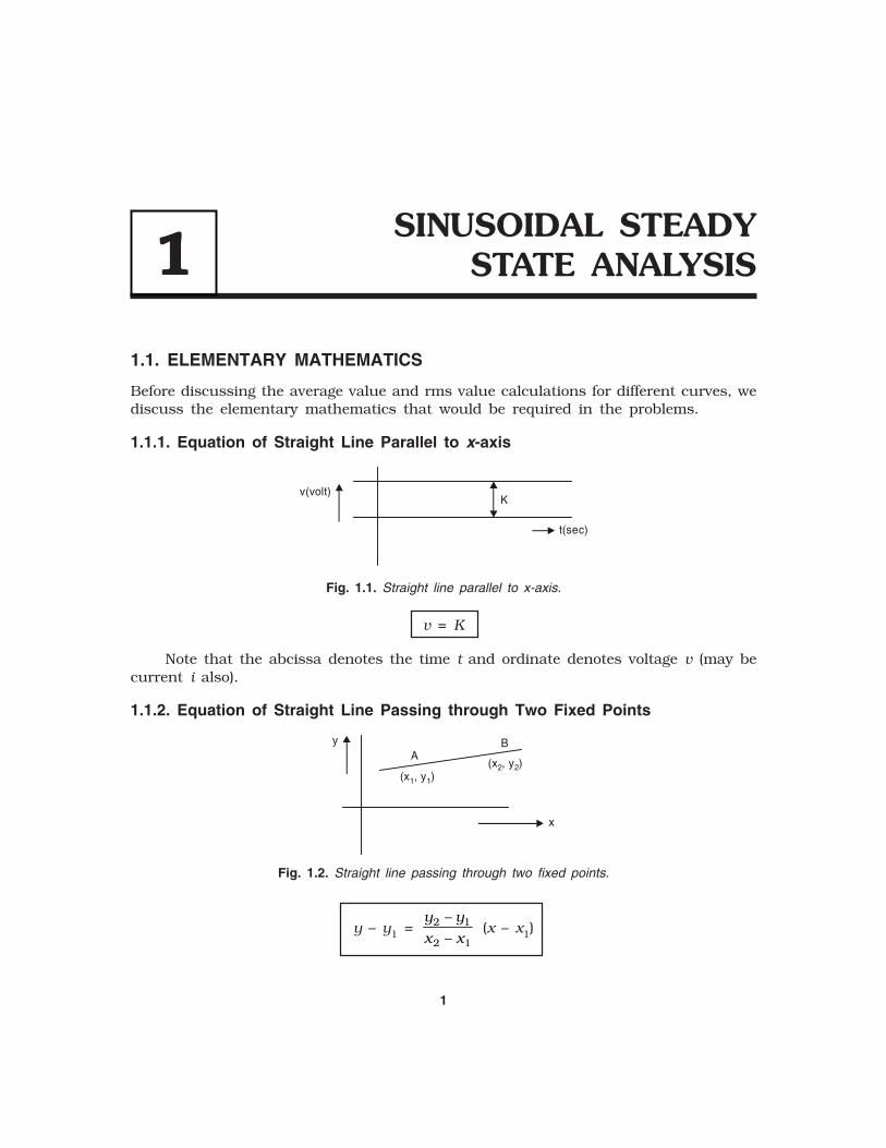
1.1.1. Equation of Straight Line Parallel to x-axis

t(sec)

Kv(volt)

Fig. 1.1. Straight line parallel to x-axis.

v = K

Note that the abcissa denotes the time t and ordinate denotes voltage v (may becurrent i also).

1.1.2. Equation of Straight Line Passing through Two Fixed Points

(x , y )1 1

(x , y )2 2

yA

B

x

Fig. 1.2. Straight line passing through two fixed points.

y – y1 = y y

x x2 1

2 1

–

– (x – x1)

1

11111

2 ELECTRICAL ENGINEERING

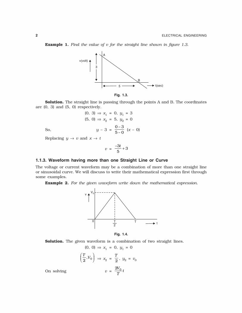
Example 1. Find the value of v for the straight line shown in figure 1.3.

v(volt)

t(sec)

3

B

A

5

Fig. 1.3.

Solution. The straight line is passing through the points A and B. The coordinatesare (0, 3) and (5, 0) respectively.

(0, 3) ⇒ x1 = 0, y1 = 3

(5, 0) ⇒ x2 = 5, y2 = 0

So, y – 3 =0 35 0

––

(x – 0)

Replacing y → v and x → t

v =–3t

53+

1.1.3. Waveform having more than one Straight Line or Curve

The voltage or current waveform may be a combination of more than one straight lineor sinusoidal curve. We will discuss to write their mathematical expression first throughsome examples.

Example 2. For the given waveform write down the mathematical expression.

vV0

0 T tT2

Fig. 1.4.

Solution. The given waveform is a combination of two straight lines.

(0, 0) ⇒ x1 = 0, y1 = 0

TV

2 0,FHG

IKJ ⇒ x2 =

T

2, y2 = v0

On solving v =2VT

t0

SINUSOIDAL STEADY STATE ANALYSIS 3

v

(0, 0) t

T2

, V0 v

t

T2

, V0

(T, 0)

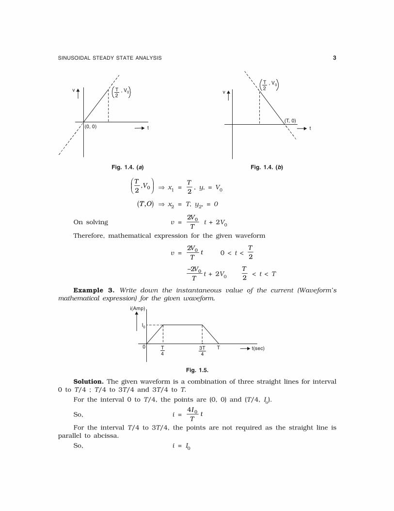
Fig. 1.4. (a) Fig. 1.4. (b)

TV

2 0,FHG

IKJ ⇒ x1 =

T

2, y, = V0

� ��b g ⇒ x2 = T, y2, = 0

On solving v =2 0V

T t + 2V0

Therefore, mathematical expression for the given waveform

v =2 0V

Tt 0 < t <

T

2

–2VT

0 t + 2V0

T

2 < t < T

Example 3. Write down the instantaneous value of the current (Waveform’smathematical expression) for the given waveform.

I0

0 T4

3T4

T t(sec)

i(Amp)

Fig. 1.5.

Solution. The given waveform is a combination of three straight lines for interval0 to T/4 ; T/4 to 3T/4 and 3T/4 to T.

For the interval 0 to T/4, the points are (0, 0) and (T/4, Io).

So, i =4 0I

Tt

For the interval T/4 to 3T/4, the points are not required as the straight line isparallel to abcissa.

So, i = I0

4 ELECTRICAL ENGINEERING

For the interval 3T/4 to T, the points are 34 0T

I,FHG

IKJ and (T, 0)

So, i =4 0I

Tt + 4I0

Therefore, i =4 0I

Tt 0 < t <

T

4

I0T

4< t

T< 34

–4I

Tt0 + 4I0

34T

< t < T

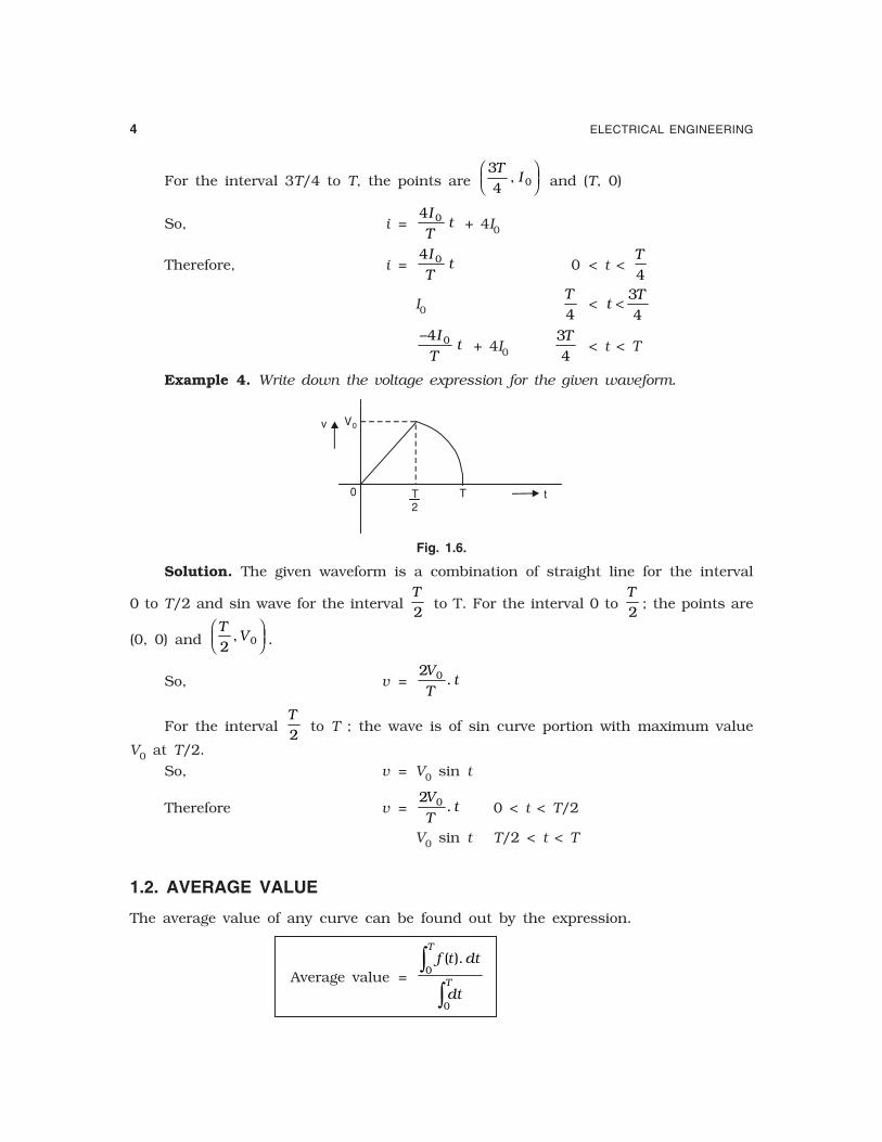
Example 4. Write down the voltage expression for the given waveform.

v

t

V0

0 T2

T

Fig. 1.6.

Solution. The given waveform is a combination of straight line for the interval

0 to T/2 and sin wave for the interval T

2 to T. For the interval 0 to

T

2; the points are

(0, 0) and T

V2 0,FHG

IKJ .

So, v =2 0V

Tt.

For the interval T

2 to T ; the wave is of sin curve portion with maximum value

V0 at T/2.

So, v = V0 sin t

Therefore v =2 0V

Tt. 0 < t < T/2

V0 sin t T/2 < t < T

1.2. AVERAGE VALUE

The average value of any curve can be found out by the expression.

Average value =f t dt

dt

T

T

( ).0

0

z

z

SINUSOIDAL STEADY STATE ANALYSIS 5

Where, f (t) = Mathematical expression for the given curve.

Tips–1. If the curve has line of symmetry (refer figure of example 2, the triangular

wave has line of symmetry at t =T

2.

then, Average value =f t dt

dt

T

T

( )./

/0

2

0

2

z

zTips–2. If the Mathematical expression is splitting for different time intervals, the

integration is done by parts (refer example 5)

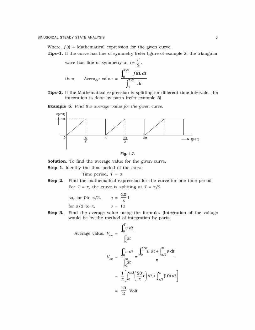
Example 5. Find the average value for the given curve.

0

10

v(volt)

t(sec)π2

π 2π3π2

Fig. 1.7.

Solution. To find the average value for the given curve,

Step 1. Identify the time period of the curve

Time period, T = πStep 2. Find the mathematical expression for the curve for one time period.

For T = π, the curve is splitting at T = π/2

so, for 0to π/2, v =20π

t

for π/2 to π, v = 10

Step 3. Find the average value using the formula. (Integration of the voltagewould be by the method of integration by parts,

Average value, Vav =v dt

dt

T

T0

0

z

z

Vav =v dt

dt

v dt v dt0

0

20

2π

ππ

ππ

πz

z

zz=

+/

/

=1 20

1020

2

π π π

ππt dt dt

FHG

IKJ

+L

NM

O

QPzz ( )

/

/

=152

Volt

6 ELECTRICAL ENGINEERING

Example 6. Find the average value for the curve given in example 4.

Solution. For the curve of example 4.

Step 1. Time period, T = T

Step 2. v =2 0V

Tt. 0 < t < T/2

V0 Sin t T/2 < t < T

Step 3. Vav =v dt

dt

T

T0

0

z

z

=

2

0

00

20

2 VT

t dt V t dt

T

T

TT FHG

IKJ

+ zz sin

–

/

/b g

=1 2

2 40 20

2

0T

V

T

TV T T– – cos cos /

L

NMM

O

QPP

+ +L

NMM

O

QPP

b g

=V V

T

TT0 0

4 2+ F

HGIKJ

cos – cos

Tips if T is 2π (given),

Vav =V V0 0

4 2+

π (cos π – cos 2π)

=V V

V0 004

22

14

1068+ = F

HGIKJ

=π π

– –0. *

So, Vav = 0.068

The average value is negative so we will take the positive value, as average valueis always positive.

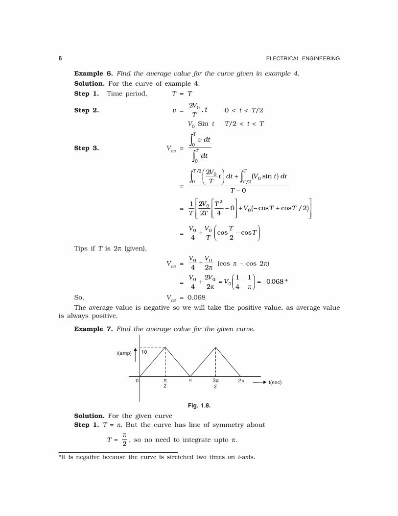
Example 7. Find the average value for the given curve.

0

10i(amp)

t(sec)π2

π 2π3π2

Fig. 1.8.

Solution. For the given curveStep 1. T = π, But the curve has line of symmetry about

T = π2

, so no need to integrate upto π.

*It is negative because the curve is stretched two times on t-axis.

SINUSOIDAL STEADY STATE ANALYSIS 7

i.e., Iav =i dt

dt

0

2

0

2

π

π

/

/

z

z

Step 2. For the internal 0 to π2

(No need to find the expression for time intervalπ2

to π).

i = ��

π t 0 < t < π�

Step 3. Iav =

200

2

0

2

ππ

π

t dt

dt

FHG

IKJz

z

/

/ = 5 amp

1.3. RMS VALUEThe rms value of any curve can be calculated by the expression.

Rms value =f t dt

dt

T

T

b gn s2

0

0

z

z

The difference in rms value from average value is only square of the function beforeintegration and finally under root of the complete expression.

Therefore, all the steps followed in calculating average value is same for rms valuetoo. The only difference is in step 3 where the different formula is used for calculatingrms value.

Example 8. Repeat the example 5 for rms voltage.

Solution. Step 1 and Step 2 are same.

i.e., T = π

v =20π

t 0 < t < π/2

10 π/2 < t < π

Step 3. Vrms =( )v dt

dt

2

0

0

π

πz

z

=

2010

22

20

2

0

π π

ππ

π

t dt dt

dt

FHG

IKJ

+ zz

z

( )/

/

= 65.9 Volt

8 ELECTRICAL ENGINEERING

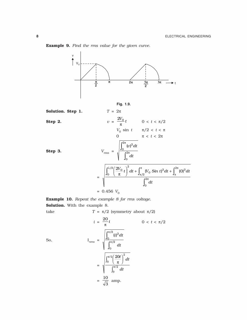
Example 9. Find the rms value for the given curve.

v

t

V0

π2π2

ππ 2π2π 3π3π5π5π22

Fig. 1.9.

Solution. Step 1. T = 2π

Step 2. v =2 0V

tπ

0 < t < π/2

V0 sin t π/2 < t < π0 π < t < 2π

Step 3. Vrms =( )v dt

dt

2

0

2

0

2

π

πz

z

=

2 02

02 2

2

20

2

0

2

Vt dt V Sin t dt dt

dt

π π

π

π

πλ

π

FHG

IKJ

+ + zzz

z

( ) (0)/

/

= 0.456 V0

Example 10. Repeat the example 8 for rms voltage.

Solution. With the example 8.

take T = π/2 (symmetry about π/2)

i =20π

t 0 < t < π/2

So, Inms =( )

/

/

i dt

dt

2

0

2

0

2

π

πz

z

=

���

�

�

�

�

���

��

ππ

π

FHG

IKJz

z

�

�

=10

3 amp.

Electrical Engineering by R K Rajput

Publisher : Laxmi Publications ISBN : 9788131805817 Author : R K Rajput

Type the URL : http://www.kopykitab.com/product/3082

Get this eBook

10%OFF