Electrical Power System Analysis 3. the Admittance Model and Network

Electrical Power System Analysis

The Admittance Model and Network Calculations

Dr : Houssem Rafik El- Hana BOUCHEKARA

2010/2012 1432/1433

KINGDOM OF SAUDI ARABIA Ministry Of High Education

Umm Al-Qura University College of Engineering & Islamic Architecture

Department Of Electrical Engineering


Dr Houssem Rafik El Hana Bouchekara 2

Contents

3 THE ADMITTANCE MODEL AND NETWORK CALCULATIONS........................................... 3

3.1 BRANCH AND NODE ADMITTANCES .................................................................................... 3

3.2 MUTUALLY COUPLED BRANCHES IN .......................................................................... 9

3.3 AN EQUIVALENT ADMITTANCE NETWORK .......................................................................... 14

3.4 MODIFICATION OF .............................................................................................. 17

3.5 THE NETWORK INCIDENCE MATRIX AND ................................................................. 19

3.6 THE METHOD OF SUCCESSIVE ELIMINATION ....................................................................... 23

3.7 NODE ELIMINATION (KRON REDUCTION) .......................................................................... 30

3.8 TRIANGULAR FACTORIZATION .......................................................................................... 32

3.9 SPARSITY AND NEAR-OPTIMAL ORDERING ......................................................................... 36

3.10 SUMMARY ................................................................................................................... 37

3.11 PROBLEMS ................................................................................................................... 37



3 THE ADMITTANCE MODEL AND NETWORK CALCULATIONS

The typical power transmission network spans a large geographic area and involves a

large number and variety of network components. The electrical characteristics of the

individual components are developed in previous chapters and now we are concerned with

the composite representation of those components when they are interconnected to form

the network. For large-scale system analysis the network model takes on the form of a

network matrix. With elements determined by the choice of parameter.

There are two choices. The current flow through a network component can be

related to "the voltage drop across it by either an admittance or an impedance parameter.

This chapter treats the admittance representation in the form of a primitive model which

describes the electrical characteristics of the network components. The primitive model

neither requires nor provides any information about how the components are

interconnected to form the network.

The steady-state behavior of all the components acting together as a system is given

by the nodal admittance matrix based on nodal analysis o f the network equations.

The nodal admittance matrix of the typical power system is large and sparse, and

can be constructed in a systematic building-block manner; The building-block approach

provides insight for developing algorithms to account for network changes. Because the

network matrices are very large, sparsity techniques are needed to enhance the

computational efficiency of computer programs employed in solving many of the power

system problems described in later chapters.

The particular importance of the present chapter, and also Chap.4, which develops

the nodal impedance matrix, becomes evident in the course of power-flow and fault analysis

of the system.

3.1 BRANCH AND NODE ADMITTANCES

In per-phase analysis the components of the power transmission system are

modeled and represented by passive impedances or equivalent admittances accompanied,

where appropriate, by active voltage or current sources. In the steady state, for example, a

generator can be represented by the circuit of either Figure 1 (a) or Figure 1 (b). The circuit

having the constant emf series impedance , and terminal voltage V has the voltage

equation

(1)

Dividing across by gives the current equation for Figure 1 (b)

(2)

where Thus, the emf and its series impedance can be

interchanged with the current source and its shunt admittance , provided



(3)

Figure 1: Circuits illustrating the equivalence of sources when

Sources such as and may be considered externally applied at the nodes of the

transmission network, which then consists of only passive branches. In this chapter

subscripts and distinguish branch quantities from node quantities which have subscripts

and q or else numbers. For network modeling we may then represent the typical

branch by either the branch impedance or the branch admittance , whichever is more

convenient. The branch impedance is often called the primitive impedance, and likewise,

is called the primitive admittance. The equations characterizing the branch are

(4)

where is the reciprocal of and is the voltage drop across the branch in the

direction of the branch current . Regardless of how it is connected into the network, the

typical branch has the two associated variables and related by Eqs (4).

In this chapter we concentrate on the branch admittance form in order to establish

the nodal admittance representation of the power network, and Chap. 4 treats the

impedance form.

In Sec. 1.12 rules are given for forming the bus admittance matrix of the network.

Review of those rules is recommended since we are about to consider an alternative method

for formation. The new method is more general because it is easily extended to

networks with mutually coupled elements. Our approach first considers each branch

separately and then in combination with other branches of the network.

Suppose that only branch admittance is connected between nodes and as

part of a larger network of which only the reference node appears in Figure 2. Current

injected into the network at any node is considered positive and current leaving the network

at any node is considered negative. In Figure 2 current is that portion or the total current

injected into node which passes through Likewise, is that portion of the current

injected into node which passes through . The voltages and are the voltages of

nodes and ,respectively, measured with respect to network reference. By Kirchhoff's

law at node and , at node . These two current equations arranged in

vector form are



(5)

Figure 2: Primitive branch voltage drop , branch current , injected currents and , node voltages

and , with respect to network reference.

In E q. (5) the labels or pointers and associate the direction of from node

to node with the entries and , which are then said to be in row and row ,

respectively. In a similar manner, the voltage drop in the direction of has the equation

or expressed in vector form

(6)

Substituting this expression for in the admittance equation gives

(7)

and premultiplying both sides of Eq. (6) by the column vector of Eq. (5) , we obtain

(8)

which, simplifies to

(9)

This is the nodal admittance equation for branch and the coefficient matrix is the

nodal admittance matrix. We note that the off-diagonal elements equal the negative of the

branch admittance. The matrix of Eq. (8) is singular because neither node nor node

connects to the reference. In the particular case where one of the two nodes, say, , is the

reference node, then node voltage

is zero and Eq. (9) reduces to the 1 x 1 matrix equation

(10)

corresponding to removal of row and column from the coefficient matrix.



Despite its straight forward derivation, Eq.(9) and the procedure leading to it are

important in more general situations. We note that the branch voltage is transformed to

the node voltages and , and the branch current is likewise represented by the

current injections and The coefficient matrix relating the node voltages and currents

of Eq. (9) follows from the fact that in Eq. (8)

(11)

This 22 matrix is an important building block for representing more general

networks, as we shall soon see. The row and column pointers identify each entry in the

coefficient matrix by node numbers. For instance, in the first row and second column of Eq.

(11) the entry -1 is identified with nodes and of Figure 2 and the other entries are

similarly identified.

Thus, the coefficient matrices of Eqs.(9) and (10) are simply storage matrices with

row and column labels determined by the end nodes of the branch. Each branch of the

network has a similar matrix labeled according to the nodes of the network to which that

branch is connected. To obtain the overall nodal admittance matrix of the entire network,

we simply combine the individual branch matrices by adding together elements with

identical row and column labels. Such addition causes the sum of the branch currents

flowing from each node of the network to equal the total current injected into that node, as

required by Kirchhoff's current law. In the overall matrix, the off-diagonal element is the

negative sum of the admittances connected between nodes ⓘ and ⓙ and the diagonal

entry is the algebraic sum of the admittances connected to node ⓘ. Provided at least

one of the network branches is connected to the reference node, the net result is of

the system, as shown in the following example.

Example 1:

The single-line diagram of a small power system is shown in Figure 3. The

corresponding reactance diagram, with reactance specified in per unit, is shown in Figure 4.

A generator with emf equal to per unit is connected through a transformer to high-

voltage node ③, while a motor with internal voltage equal to ° is similarly

connected to node ④· Develop the nodal admittance matrix for each of the network

branches and then write the nodal admittance equations of the system.



Figure 3: Single-line diagram of the four-bus system of Example 1.Reference node is not shown.

Figure 4: Reactance diagram for Figure 3. Node is reference, reactances and voltages at per unit.

Solution:

Figure 5: Per- unit admittance diagram for Figure 4 with current sources replacing voltage sources. Branch

names to correspond to the subscripts of branch voltages and currents.



The reactances of the generator and the motor may be combined with the

irrespective step-up transformer reactances. Then, by transformation of sources the

combined reactances and the generated emfs are replaced by the equivalent current

sources and shunt admittances shown in Figure 5. We will treat the current sources as

external injections at nodes ③ and ④ and name the seven passive branches according to

the subscripts of their currents and voltages. For example, the branch between nodes

and ③ will be called branch . The admittance of each branch is simply the reciprocal of the

branch impedance and Figure 5 shows the resultant admittance diagram with all values in

per unit. The two branches and g connected to the reference node are characterized by

Eq. (10), while Eq (9) applies to each of the other five branches. By setting and in those

equations equal to the node numbers at the ends of the individual branches of Figure 5, we

obtain

③

③

③

③

③ ③

④ ④

④ ④

④

④

The order in which the labels are assigned is not important here, provided the

columns and rows follow the same order. However, for consistency with later sections let us

assign the node numbers in the directions of the branch currents of Figure 5, which also

shows the numerical values of the admittances. Combining together those elements of the

above matrices having identical row and column labels gives

③ ④

③

④

Substituting then numerical values of the branch admittances into this matrix, we obtain for

the overall network the nodal admittance equations

where and are the node voltages measured with respect to the

reference node and are the

external currents injected at the system nodes.

The coefficient matrix obtained in the above example is exactly the same as the bus

admittance matrix found in Sec. 3.12 using the usual rules for formation. However, the

approach based on the building-block matrix has advantages when extended to networks

with mutually coupled branches, as we now demonstrate.



3.2 MUTUALLY COUPLED BRANCHES IN

The procedure based on the building-block matrix is now extended to two mutually

coupled branches which are part of a larger network but which are not inductively coupled

to any other branches. In Sec. 2.2 the primitive equations of such mutually coupled branches

are developed in the form of Eq.2.24 for impedances and Eq.2.26 for admittances. The

notation is different here because we are now using numbers to identify nodes rather than

branches.

Assume that branch impedance connected between nodes and is coupled

through mutual impedance to branch impedance connected between node's ⓟ and

ⓠ of Figure 6. The voltage drops and due to the branch currents and then given

by the primitive impedance equation corresponding to Eq.2.24 in the form

(12)

in which the coefficient matrix is symmetrical. The mutual impedance is

considered positive when currents and enter the terminals marked with clots in Figure

6 (a); the voltage drops and then have the polarities shown. multiplying Eq. (12) by the

inverse of the primitive impedance matrix

(13)

Figure 6: Two mutually coupled branches with (a) impedance parameters and (b) corresponding admittances.

we obtain the admittance form of Eq.(26) for the two branches

(14)

which is also symmetrical. The admittance matrix of Eq.(14) called the primitive

admittance matrix of the two coupled branches, corresponds to Figure 6 (b). The primitive



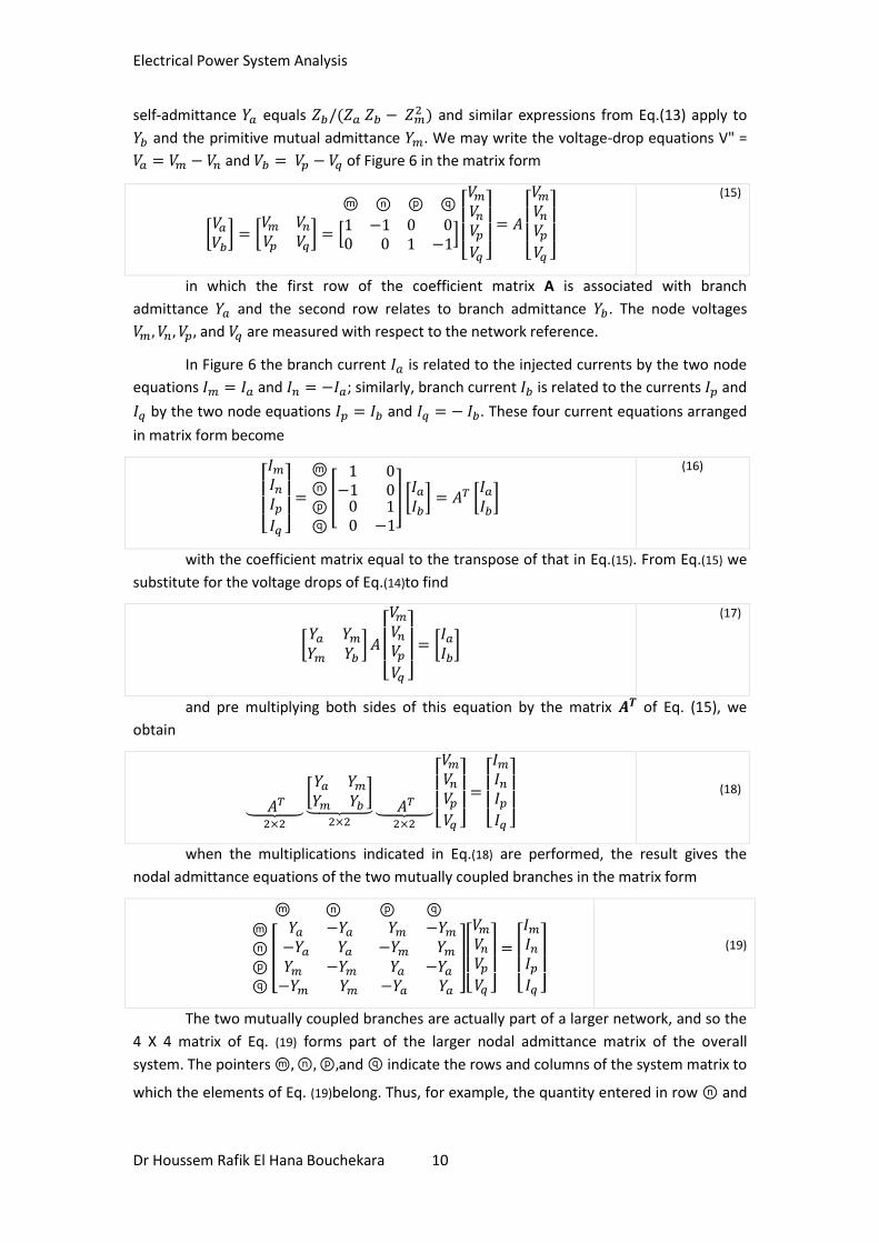
self-admittance equals and similar expressions from Eq.(13) apply to

and the primitive mutual admittance . We may write the voltage-drop equations V" =

and of Figure 6 in the matrix form

ⓟ ⓠ

(15)

in which the first row of the coefficient matrix A is associated with branch

admittance and the second row relates to branch admittance . The node voltages

and are measured with respect to the network reference.

In Figure 6 the branch current is related to the injected currents by the two node

equations and ; similarly, branch current is related to the currents and

by the two node equations and . These four current equations arranged

in matrix form become

ⓟ

ⓠ

(16)

with the coefficient matrix equal to the transpose of that in Eq.(15). From Eq.(15) we

substitute for the voltage drops of Eq.(14)to find

(17)

and pre multiplying both sides of this equation by the matrix of Eq. (15), we

obtain

(18)

when the multiplications indicated in Eq.(18) are performed, the result gives the

nodal admittance equations of the two mutually coupled branches in the matrix form

ⓟ ⓠ

ⓟ

ⓠ

(19)

The two mutually coupled branches are actually part of a larger network, and so the

4 X 4 matrix of Eq. (19) forms part of the larger nodal admittance matrix of the overall

system. The pointers ⓟ and ⓠ indicate the rows and columns of the system matrix to

which the elements of Eq. (19)belong. Thus, for example, the quantity entered in row and



column ⓟ of the system nodal admittance matrix is and similar entries are made from

the other elements of Eq. (19).

The nodal admittance matrix of the two coupled branches may be formed directly by

inspection. This becomes clear when we write the coefficient matrix of Eq.(19) in the

alternative form

ⓟ ⓠ

ⓟⓠ

ⓟ ⓠⓟⓠ

(20)

To obtain Eq. (20), we multiply each element of the primitive admittance matrix by

the 22 building-block matrix. The labels assigned to the rows and columns of the

multipliers in Eq.(20) are easily determined. First, we note that the self-admittance is

measured between nodes and with the dot at node . Hence, the 2X2 matrix

multiplying in Eq. (20) has rows and columns labeled and in that order. Then, the

self-admittance between nodes ⓟ and ⓠ is multiplied by the 2X2 matrix with labels ⓟ

and ⓠ in the order shown since node ⓟ is marked with a dot. Finally, the labels of the

matrices multiplying the mutual admittance are assigned row by row and then column

by column so as to align and agree with those already given to the self-inductances. In the

nodal admittance matrix of Eqs.(19) and (20) the sum of the columns (and of the rows) adds

up to zero. This is because none of the nodes ⓟ and ⓠhas been considered as the

reference node of the network. In the special case where one of the nodes, say, node , is

in fact the reference, is zero and column in Eq.(19) does not need to appear; furthermore,

does not have to be explicitly represented since the reference node current is not an

independent quantity. Consequently, when node is the reference, we may eliminate the

row and column of that node from Eqs. (19)and (20).

It is important to note that nodes , , ⓟ, and ⓠ are often not distinct. For

instance, suppose that nodes and ⓠ are one and the same node. In that case columns

and ⓠ of Eq. (19) can be combined together since , and the corresponding rows can

be added because and are parts of the common injected current. The following

example illustrates this situation.

Example 2:

Two branches having impedances equal to per unit are coupled through

mutual impedance per unit, as shown in Figure 7 Find the nodal admittance

matrix for the mutually coupled branches and write the corresponding nodal admittance

equations.



Figure 7: The two mutually coupled branches of Example 7.2, their primitive impedances and primitive

admittance sin per unit.

Solution:

The primitive impedance matrix for the mutually coupled branches of Figure 7 (a) is

inverted as a single entity to yield the primitive admittances of Figure 7(b), that is,

First, the rows and columns of the building-block matrix which multiplies the

primitive self-admittance between nodes and ③ are labeled ③ and in that order to

correspond to the dot marking node ③- Next, the rows and columns of the 2 x 2 matrix

multiplying the self-admittance between nodes and ③ are labeled and in the order

shown because node ③ is marked. Finally, the pointers of the matrices multiplying the

mutual admittance are aligned with those of the self-admittances to form the 4 x 4 array

similar to Eq. (20) as follows:

③ ③

③ ③

③ ③

③ ③

Since there are only three nodes in Figure 7, the required 3 X 1 matrix is found by

adding the columns and rows of common node ③ to obtain

③

③



Figure 8: Three branches with mutual coupling between branches and and between branches and .

The new diagonal element representing node ③, for instance, is the sum of the four

elements in rows ③ and columns ③ the previous matrix.

The three nodal admittance equations in vector-matrix form are then written

where and are the voltages at nodes , and ③ measured with respect

to reference, while and are the external currents injected at the respective nodes.

As in Sec.3.1, the coefficient matrix or the last equation can be combined with the

nodal admittance matrices of the other branches of the network In order to obtain the nodal

admittance matrix of the entire system.

For three or more coupled branches we follow the same procedure as above. For

example, the three coupled branches of Figure 8 have primitive impedance and admittance

matrices given by

(21)

The zeros in the -matrix arise because branches and care not directly coupled. For

all nonzero values of the current la of Figure 8, branches and are indirectly coupled

through branch , as shown by nonzero of the primitive admittance matrix.

Therefore, to form for a network which has mutually coupled branches, we do

the following in sequence:

1. Invert the primitive impedance matrices of the network branches to obtain

the corresponding primitive admittance matrices. A single branch has a 1 x 1

matrix, two mutually coupled branches have a 2 X 2 matrix, three mutually

coupled branches have a 3 x 3 matrix, and soon.

2. Multiply the elements of each primitive admittance matrix by the 2 X 2

building-block matrix.

3. label the two rows and the two columns of each diagonal building-block

matrix with the end-node numbers of the corresponding self-admittance.



For mutually coupled branches it is important to label in the order of the

marked (dotted) - then – unmarked (undotted) node numbers.

4. Label the two rows of each off-diagont building-block matrix with node

numbers aligned consistent with the row labels assigned in ③; then label

the columns consistent with the column labels of ③.

5. Combine. by adding together, those elements with identical row and column

labels to obtain the nodal admittance matrix of the overall network. If one of

the nodes encountered is the reference node, omit its row and column to

obtain the system .

3.3 AN EQUIVALENT ADMITTANCE NETWORK

We have demonstrated how to write the nodal admittance equations for one branch

or a number of mutually coupled branches which are part of a larger network. We now show

that such equations can be interpreted as representing an equivalent admittance network

with no mutually coupled elements. This may be useful when forming for an original

network having mutually coupled elements.

The currents injected into the nodes of Figure 6,are described in terms of node

voltages and admittances by Eq. (19). For example, the equation for the current at node

③ is given by the first row of Eq. (19) as follows:

(22)

Adding and subtracting the term on the right-hand side of Eq.(22) and

combining terms with common coefficients, we obtain the Kirchhoff's current equation at

node ③

(23)

Figure 9: Developing the nodal admittance network of two mutually coupled branches.



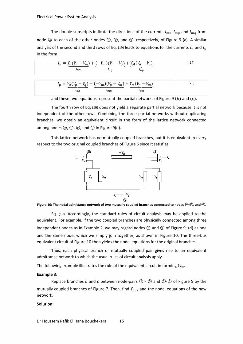
The double subscripts indicate the directions of the currents and from

node ③ to each of the other nodes , ⓟ, and ⓠ, respectively, of Figure 9 (a). A similar

analysis of the second and third rows of Eq. (19) leads to equations for the currents and

in the form

(24)

(25)

and these two equations represent the partial networks of Figure 9 and

The fourth row of Eq. (19) does not yield a separate partial network because it is not

independent of the other rows. Combining the three partial networks without duplicating

branches, we obtain an equivalent circuit in the form of the lattice network connected

among nodes , , ⓟ, and ⓠ in Figure 9(d).

This lattice network has no mutually coupled branches, but it is equivalent in every

respect to the two original coupled branches of Figure 6 since it satisfies

Figure 10: The nodal admittance network of two mutually coupled branches connected to nodes ,ⓟ, and ⓠ.

Eq. (19). Accordingly, the standard rules of circuit analysis may be applied to the

equivalent. For example, if the two coupled branches are physically connected among three

independent nodes as in Example 2, we may regard nodes and ⓠ of Figure 9 (d) as one

and the same node, which we simply join together, as shown in Figure 10. The three-bus

equivalent circuit of Figure 10 then yields the nodal equations for the original branches.

Thus, each physical branch or mutually coupled pair gives rise to an equivalent

admittance network to which the usual rules of circuit analysis apply.

The following example illustrates the role of the equivalent circuit in forming

Example 3:

Replace branches and between node-pairs - ③ and -③ of Figure 5 by the

mutually coupled branches of Figure 7. Then, find and the nodal equations of the new

network.

Solution:



The admittance diagram of the new network including the mutual coupling is shown

in Figure 11. From Example 2 we know that the mutually coupled branches have then nodal

admittance matrix

③

③

which corresponds to the equivalent circuit shown encircled in Figure 12The

remaining portion of Figure 12 is drawn from Figure 5. Since mutual coupling is not evident

in Figure 12, we may apply the standard rules of formation to the

Figure 11: Per-unit admittance diagram for Example 3.

Figure 12: Nodal admittance network for Example 3 The shaded portion represents two mutually coupled

branches connected between buses , , and ③.



③ ④

③

④

Note that the two admittances between nodes and combine in parallel to yield

3.4 MODIFICATION OF

The building-block approach and the equivalent circuits of previous section provide

important insights into the manner in which each branch self- and mutual admittance

contributes to the entries of and the corresponding equivalent network of the overall

system. As a result, it is clear that is merely a systematic means of combining the nodal

admittance matrices of the various network branches. We simply form a large array with

rows and columns ordered according to the sequence in which the no reference nodes of

the network are numbered, and within it we combine entries with matching labels drawn

from the nodal admittance matrices of the individual branches. Consequently, we can easily

see how to modify the system to account for branch additions or other changes to the

system network. For instance, to modify of the existing network to reflect the addition

of the branch admittance between the nodes and , we simply add to the elements

and of and subtract from the symmetrical elements and . In other

words, to incorporate the new branch admittance into the network, we add to the

existing the change matrix given by

(26)

Again, we recognize as a storage matrix with rows and columns marked

and . Using Eq.(26), we may change the admittance value of a single branch of the

network by adding a new branch between the same end nodes and such that the

parallel combination of the old and new branches yields the desired value. Moreover, to

remove a branch admittance already connected between nodes and of the

network, we simply add the branch admittance – between the same nodes, which

amounts to subtracting the elements of from the existing Equation (20) shows

that a pair of mutually coupled branches ,can be removed from the network by subtracting

the entries in the change matrix

③ ④

③

④

(27)



from the rows and columns of corresponding to the end nodes , ,ⓟ ,and

ⓠ. Of course, if only one of the two mutually coupled branches is to be removed from the

network, we could first remove all the entries for the mutually coupled pair from using

Eq.(27) and then add the entries for the branch to be retained using Eq.(26). Other strategies

for modifying to reflect network changes become clear from the insights developed in

Secs.3.1 through 3.3.

Example 4:

Determine the bus admittance matrix of the network of Figure 5 by removing the

effects of mutual coupling from of Figure 11.

Solution:

The for the entire system of Figure 11 including mutual coupling is found in

Example 3 to be

③ ④

③

④

To remove completely the effect of mutual coupling from the network , we

proceed in two steps by first removing the two mutually coupled branches altogether

and then restoring each of the two branches without mutual coupling between them.

To remove the two mutually coupled branches from the network, we subtract from the

system the entries in

③ ④

③

④

corresponding to the encircled portion of Figure 12.

Now we must reconnect to the network the uncoupled branches, each of which

has an admittance per unit. Accordingly, to reconnect the branch

between nodes and ③, we add to the change matrix

③ ④

③

④

and similarly for the branch between nodes and ③ we add and



③ ④

③

④

Appropriately subtracting and adding the three change matrices and the original give

the new bus admittance matrix for the uncoupled branches

③ ④

③

④

–

which agrees with Example 1.

3.5 THE NETWORK INCIDENCE MATRIX AND

In Secs. 3.1 and 3.2 nodal admittance equations for each branch and mutually

coupled pair of branches are derived in dependently from those of other branches in the

network. The nodal admittance matrices of the individual branches are then combined

together in order to build of the overall system. Since we now understand the process,

we may proceed to the more formal approach which treats all the equations of the system

simultaneously rather than separately. We will use the example system of Figure 11 to

establish the general procedure.

Two of the seven branches in Figure 11 are mutually coupled as shown. The mutually

coupled pair is characterized by Eq.(14) and the other five branches by Eq.(4). Arranging the

seven branch equations into an array format, we obtain

(28)

The coefficient matrix is the primitive admittance matrix formed by inspection of

Figure 11. Each branch of the network contributes a diagonal entry equal to the simple

reciprocal of its branch impedance except for branches and , which are mutually coupled

and have entries determined by Eq.(13). For the general case Eq. (28) may be more

compactly written in the form

(29)

where and are the respective column vectors of branch voltages and

currents, while represents the primitive admittance matrix of the network. The primitive

equations do not tell how the branches are configured within the network. The geometrical

configuration of the branches, called the topology, is provided by a directed graph, as shown

in Fig.7.l3 in which each branch of the network of Figure 11 is represented between its



end nodes by a directed line segment with an arrow in the direction of the branch current.

When a branch connects to a node, the branch and node are said to be incident. A tree of a

graph is formed by those branches of the graph which interconnect or span all the nodes of

the graph without forming any closed path. In general, there are many possible trees of a

network since different combinations of branches can be chosen to span the nodes. Thus,

for example, branches and in Figure 13 (6) define a tree. The remaining branches

and are called links, and when a link is added to a tree, a closed path or loop is

formed.

Figure 13: The linear graph for Fig.7.11 showing: directed-line segments for branches; (b) branches, a, b, c, and define a tree while branches , , and are links.

A graph may be described in terms of a connection or incidence matrix. Of particular

interest is the branch-to-node incidence matrix , which has one row for each branch and

one column for each node with an entry in row and column according to the following

rule:

ⓙ

ⓙ

ⓙ

(30)

This rule formalizes for the network as a whole the procedure used to set up the

coefficient matrices of Eqs.(6) and (15) for the individual branches. In network calculations we

usually choose a reference node. The column corresponding to the reference node is then

omitted from and the resultant matrix is denoted by . For example, choosing node ⓪ as

the reference in Figure 13 and invoking the rule of Eq.(30), we obtain the rectangular

branch-to-node matrix

③ ④

(31)

The no reference nodes of a network are often called independent nodes or buses,

and when we say that the network has buses, we generally mean that there are

independent nodes not including the reference node. The matrix has the row-column

dimension for any network with branches and nodes excluding the reference.

We note that each row of Eq.(31) has two nonzero entries which add to zero except for rows



and , each of which has only one nonzero entry. This is because branches and of

Figure 11 have one end connected to the reference node for which no column is shown.

The voltage across each branch may be expressed as the difference in its end-bus

voltages measured with respect to the reference node. For example, in Figure 11 the

voltages at buses , , ③, and ④ with respect to reference node ⓪ are denoted by

and , respectively, and so the voltage drops a cross the branches are given by

or

in which the coefficient matrix is the A matrix of Eq.(31). This is one illustration of

the general result for any network given by

(32)

where is the B X 1 column vector of branch voltage drops and is the N X 1

column vector of bus voltages measured with respect to the chosen reference node.

Equations (6) and (15) are particular applications of Eq.(32) to individual branches. We further

note that Kirchhoff's current law at nodes to ④ of Figure 11 yields

where and are the external currents injected

at nodes ③ and ④, respectively. The coefficient matrix in this equation is . Again, this is

illustrative of a general result applicable to every electrical network since it simply states, in

accordance with Kirchhoff's current law, that the sum of all the branch currents incident to a

node of the network equals the injected current at the node. Accordingly, we may write

(33)

where is the B X 1 column vector of branch currents and I is the N X 1 column

vector with a nonzero entry for each bus with an external current source. Equations (5) and

(16) are particular examples of Eq.(33).

The matrix fully describes the topology of the network and is independent of the

particular values of the branch parameters. The latter are supplied by the primitive

admittance matrix. Therefore, two different network configurations employing the same

branches will have different matrices but the same . On the other hand, if changes



occur in branch parameters while maintaining the same network configuration, only is

altered but not .

Multiplying Eq.(29) by , we obtain

(34)

The right-hand side of Eq.(34) equals and substituting for from Eq.(32), we

fined

(35)

We may write Eq.(35) in the more concise form

(36)

where the N X N bus admittance matrix for the system is given by

(37)

has one row and one column for each of the buses in the network, and so the

standard form of the four independent equations of the example system of Figure 11 is

(38)

The four unknowns are the bus voltages and when the bus-injected

currents and are specified. Generally, is symmetrical, in which case taking the

transpose of each side of Eq.(37) shows that is also symmetrical.

Example 5:

Determine the per-unit bus admittance matrix of the example system of Figure 11

using the tree shown in Figure 13 with reference node ⓪.

Solution:

The primitive admittance matrix describing the branch admittances is given by

Eq.(28) and the branch-to-node incidence matrix for the specified tree is given by Eq.

(31)Therefore, performing the row-by-column multiplications for indicated by

we obtain the intermediate result



which we may now post multiply by to calculate

③ ④

③

④

Since currents are injected at only buses ③ and ④, the nodal equations In matrix

form are written

Example 6:

Solve the node equations of Example 5 to find the bus voltages by inverting the bus

admittance matrix.

Solution:

Pre multiplying both sides of the matrix nodal equation by the inverse of the bus

admittance matrix (determined by using a standard program on a computer or calculator)

yields

Performing the indicated multiplications, we obtain the per-unit results

3.6 THE METHOD OF SUCCESSIVE ELIMINATION

In industry-based studies of power systems the networks being solved are

geographically extensive and often encompass many hundreds of substations, generating

plants and load centers. The matrices for these large networks of thousands of nodes

have associated systems of nodal equations to be solved for a correspondingly large number

of unknown bus voltages. For such solutions computer-based numerical techniques are

required to avoid direct matrix inversion, thereby minimizing computational effort and

computer storage. The method of successive elimination, called gaussian elimination,



underlies many of the numerical methods solving the equations of such large-scale power

systems.

We now describe this method using the nodal equations of the four-bus system

(39)

(40)

(41)

(42)

Gaussian elimination consists of reducing this system of four equations in the four

unknowns , , and to a system of three equations in three unknowns and then to a

reduced system of two equations in two unknowns, and so on until there remains only one

equation in one unknown. The final equation yields a value for the corresponding unknown,

which is then substituted back in the reduced sets of equations to calculate the remaining

unknowns. The successive elimination of unknowns in the forward direction is called

forward elimination and the substitution process using the latest calculated values is called

back substitution. Forward elimination begins by selecting one equation and eliminating

from this equation one variable whose coefficient is called the pivot. We exemplify the

overall procedure by first eliminating from Eqs. (39) through (42) as follows:

Step 1

1. Divide Eq. (39) by the pivot to obtain:

(43)

2. Multiply Eq. (43) by , , and and subtract the results from Eqs. (40)

through (42), respectively, to get

(44)

(45)

(46)

Equations (43)through (46) may be written more compactly in the form

(47)

(48)

(49)

(50)

where the superscript denotes the Step 1 set of derived coefficients



(51)

and the modified right-hand side expressions.

(52)

Not e that Eqs . (48) through (50) may now be solved for , , and since has

been eliminated; and the coefficients constitute a reduced 33 matrix, which can be

interpreted as representing a reduced equivalent network with bus absent . In this three-

bus equivalent the voltages , , and have exactly the same values as in the original

four-bus system . Moreover, the effect of the current injection on the network is taken

into account at buses , ③ and ④, as shown by Eq (52). The current at bus is

multiplied by the factor – before being distributed, so to speak, to each bus ⓙ still in

the network.

We next consider the elimination or the variable .

Step 2

1. Divide Eq. (48) by the new pivot to obtain

(53)

2. Multiply Eq. (53) by

l and

and subtract the resu lts from Eqs. (49) and

(50)to get

(54)

(55)

In a manner similar to that of Step 1, we rewrite Eqs. (53) through (55) in the form

(56)

(57)

(58)

where the second set of calculated coefficients is given by

(59)

and the net currents injected at buses ③a n d ④ are



(60)

Equations (57)and (58)describe a further reduced equivalent network having only

buses ③ and ④. Voltages and are exactly the same as those of the original four-bus

network because the current injections

and

represent the effects of all the original

current sources.

We now consider elimination of the variable .

Step 3

1. Divide Eq. (57)by the pivot

to obtain

(61)

Multiply Eq. (61) by

and subtract the result from Eq. (58) to obtain

(62)

in which we have defined

(63)

Equation (62) describes t h e single equivalent branch admittance

with voltage

V4 from bus ④ to reference caused by the equivalent injected current

.

The final step in the forward elimination process yields .

Step 4

1. Divide Ea. (62) by

to obtain

(64)

At this point we have found a value for bus voltage which can be substituted back

in Eq. (61) to obtain a value for . Continuing this process of back substitution using the

values of and in Eq. (56), we obtain and then solve for from Eq. (47).

Thus, the gaussian-elimination procedure demonstrated here for a four-bus system

provides a systematic means of solving large systems of equations without having to invert

the coefficient matrix. This is most desirable when a large-scale power system is being

analyzed. The following example numerically illustrates the procedure.

Example 7:

Using gaussian elimination, solve the nodal equations of Example 5 to find the bus

voltages. At each step of the solution find the equivalent circuit of the reduced coefficient

matrix.



Solution:

In Example 5:Example 5 the nodal admittance equations in matrix form are found to

be

③ ④

③

④

To eliminate the variable from rows 2, 3, and 4, we first divide the first row by the

pivot to obtain

We now use this equation to eliminate the entry in (row 2, column 1)

of , and in the process all the other elements of row 2 are modified. Equation (51) shows

the procedure. For example, to modify the element j2.50 underlined in (row 2, column 3),

subtract from it the product of the elements enclosed by rectangles divide d by the pivot

; that is,

Similarly, the other elements of new row 2 are:

Figure 14: The equivalent three-bus network following Step 1 of Example 7 . 7.

Modified elements of rows 3 and 4 are likewise found to yield



Because , no current is distributed from bus to the remaining buses , ③

and ④ and so the currents ,

, and in the right-hand-side vector have the same values

before and after Step 1 . The partitioned system of equations involving the unknown

voltages , , and corresponds to the three-bus equivalent network constructed in Fig.

7.14 from the reduced coefficient matrix.

Step 2

Forward elimination applied to the partitioned 3 3 system of the last equation

proceeds as in Step 1 to yield

Figure 15: The equivalent two – bus network following Step 2 of Example 7.7.

in which the injected currents and

of Step 2 are also unchanged because

. At this stage we have eliminated and from the original 4 4 system of

equations and there remains the 2 2 system in the variables and corresponding to

of Fig. 7 . 1 5. Note that nodes and are eliminated.

Step 3

Continuing the forward elimination, we find

in which the entry for bus ③ in the right-hand-side vector is calculated to be

and the modified current at bus ④ is given by



Figure 7 . 1 6 (a) shows the single admittance resulting from Step 3.

Figure 16: The equivalent circuits following (a) Step 3 and (b) Step 4 o f Example 7.7.

Step4

The forward-elimination process terminates with the calculation

corresponding to the source transformation of Figure 16 (6). Therefore, forward

elimination leads to the triangular coefficient matrix given by

Since , we now begin the back-substitution process to

determine using the third row entries as follows:

which yields

Back substitution for and in the second-row equation

yields

When the calculated values o f V_2 , V_3 , and V_4 are substituted in the first-row

equation



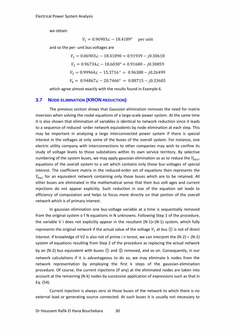
we obtain

and so the per- unit bus voltages are

–

which agree almost exactly with the results found in Example 6.

3.7 NODE ELIMINATION (KRON REDUCTION)

The previous section shows that Gaussian elimination removes the need for matrix

inversion when solving the nodal equations of a large-scale power system. At the same time

it is also shown that elimination of variables is identical to network reduction since it leads

to a sequence of reduced -order network equivalents by node elimination at each step. This

may be important in analyzing a large interconnected power system if there is special

interest in the voltages at only some of the buses of the overall system. For instance, one

electric utility company with interconnections to other companies may wish to confine its

study of voltage levels to those substations within its own service territory. By selective

numbering of the system buses, we may apply gaussian elimination so as to reduce the ,

equations of the overall system to a set which contains only those bus voltages of special

interest. The coefficient matrix in the reduced-order set of equations then represents the

for an equivalent network containing only those buses which are to be retained. All

other buses are eliminated in the mathematical sense that their bus volt ages and current

injections do not appear explicitly. Such reduction in size of the equation set leads to

efficiency of computation and helps to focus more directly on that portion of the overall

network which is of primary interest.

In gaussian elimination one bus-voltage variable at a time is sequentially removed

from the original system o f N equations in N unknowns. Following Step 1 of the procedure,

the variable V I does not explicitly appear in the resultant (N-1)(N-1) system, which fully

represents the original network if the actual value of the voltage at bus is not of direct

interest. If knowledge of V2 is also not of prime i n terest, we can interpret the (N-2) (N-2)

system of equations resulting from Step 2 of the procedure as replacing the actual network

by an (N-2) bus equivalent with buses and removed, and so on. Consequently, in our

network calculations if it is advantageous to do so, we may eliminate k nodes from the

network representation by employing the first k steps of the gaussian-elimination

procedure. Of course, the current injections (if any) at the eliminated nodes are taken into

account at the remaining (N-k) nodes by successive application of expressions such as that in

Eq. (54).

Current injection is always zero at those buses of the network to which there is no

external load or generating source connected. At such buses it is usually not necessary to



calculate the voltages explicitly, and so we may eliminate them from our representation. For

example, when i n the four-bus system, w e may write nodal admittance equations in

the form.

(65)

and following elimination of node , we obtain the 3 3 system

(66)

in which the superscripted elements of the reduced coefficient matrix are calculated

as before. Systems in which those nodes with zero current injections are eliminated are said

to be Kron (After Dr. Gabriel Kron (190 1 - 1 968) of General Electric Company, Schenectady,

NY, who contributed greatly to power system analysis) reduced. Hence, the system having t

he particular form of Eq. (65) is Kron reduced to Eq. (66), and for such systems node

elimination and Kron reduction are synonymous terms. Of course, regardless of which node

has the zero current injection, a system can be Kron reduced without having to rearrange

the equations as in Eq. (65). For example, if in the nodal equations of the N-bus

system, we may directly calculate the elements of the new, reduced bus admittance matrix

by choosing as the pivot and by eliminating bus p using the formula

(67)

where j and k take on all the integer values from 1 to N except p since row p and

column p are to be eliminated . The subscript (new) distinguishes the elements in the new

of dimension (N-1)(N-1) from the elements in the origin al .

Example 8:

Using Y22 as the initial pivot, eliminate node and the corresponding voltage V,

from the 44 system of Example 7.

Solution:

The pivot equals -j 19.25. With p set equal to 2 in Eq. (67), we may eliminate row

2 and column 2 from of Example 7 to obtain the new row 1 elements



Figure 17: The Kron -reduced network of Example 7.8.

Similar calculations yield the other elements of the Kron-reduced matrix.

Because the coefficient matrix is symmetrical, the equivalent circuit of Figure 17

applies. Further use o f Eq. (67),to eliminate node from Figure 17 leads to the Kron-

reduced equivalent circuit shown in Figure 15.

3.8 TRIANGULAR FACTORIZATION

In practical studies the nodal admittance equations o f a given large-scale power

system are solved under different operating conditions. Often in such studies the network

configuration and parameters are fixed and the operating conditions differ only because of

changes made to the external sources connected at the system buses. In all such cases the

same applies and the problem then is to solve repeatedly for the voltages

corresponding to different sets of current injections. In finding repeat solutions considerable

computational effort is avoided if all the calculations in the forward phase of the gaussian-

elimination procedure do not have to be repeated. This may be accomplished by expressing

as the product of two matrices L and U defined for the four-bus system by



(68)

The matrices L and U are called the lower- and upper-triangular factors of

because they have zero elements above and below the respective principal diagonals. These

two matrices have the remarkably convenient property that their product equals

(Problem 7 . 1 3). Thus, we can write

(69)

The process of developing the triangular matrices L and U from is called

triangular factorization since is factored into the product L U. Once is so factored,

the calculations in the forward-elimination phase of Gaussian elimination do not have to be

repeated since both L an d U are unique and do not change for a given . The entries in L

and U are formed by systematically recording the outcome of the calculations at each step

of a single pass through the forward elimination process. Thus, informing L and U, no new

calculations are involved.

This is now demonstrated for the four-bus system with coefficient matrix

③④

③ ④

(70)

When gaussian elimination is applied to the four nodal equations corresponding to

this , we note the following.

Step 1 yields results given by Eqs. (47) through (50) in which:

1. The coefficients , , , and are eliminated from the first column of

the original coefficient matrix of Eq.(70).

2. New coefficients 1, , , and are generated to replace

those in the first row of Eq.(70).

The coefficients in the other rows and columns are also altered, but we keep a

separate record of only those specified in ( 1 ) and (2) since these are the only results from

Step 1 which are neither used nor altered in Step 2 or subsequent steps of the forward

elimination process. Column 1 of L and row 1 of U in Eqs. (7.68) show the recorded

coefficients.

Step 2 yields results given by Eqs. (56) through (58) in which:

1. Coefficients

,

, and

are eliminated from the second column of the

reduced coefficient matrix corresponding to Eqs. (47) through (50).



2. New coefficients 1,

, and

are generated in Eq.(56) for the

second row.

These coefficients are not needed in the remaining steps of forward elimination, and

so we record them as column 2 of L and row 2 of U to show the Step 2 record . Continuing

this record-keeping procedure, we form columns 3 and 4 of L and rows 3 and 4 of U using

the results from Steps 3 and 4 of Sec. 3.6.

Therefore, matrix L is simply a record of those columns which are successively

eliminated and matrix U records those row entries which are successively generated at each

step of the forward stage of gaussian elimination.

We may use the triangular factors to solve the original system of equations by

substituting the product L U for in Eq. (38) to obtain

(71)

As an intermediate step in the solution of Eq. (71), we m ay replace the product UV

by a new voltage vector V' such that

(72)

Expressing Eq.(72) in full format shows that the original system of Eq. (38) is now

replaced by two triangular systems given by

(73)

And

(74)

The lower triangular system of Eq.(73) is readily solved by forward substitution

beginning with . We then use the calculated values of

, ,

and to solve Eq. (74) by

back substitution for the actual unknowns ,

, and

.

. Therefore, when changes are made in the current vector , the solution vector V is

found in two sequential steps; the first involves forward substitution using L and the second

employs back substitution using U.

Example 9:



Using the triangular factors of , determine the voltage at bus ③ of Figure 11

when the current source a t bus ④ is changed to per unit . All other

conditions of Figure 11 are unchanged.

Solution:

The for the network of Figure 11 is given in Example 7.3. The corresponding

matrix L may be assembled column by column from Example 7.7 simply by recording the

column which is eliminated from the coefficient matrix at each step of the forward

elimination procedure. Then, substituting for L and the new current vector in the equation

, we obtain

Solution by forward substitution beginning with yields

The matrix U is shown directly following Step 4 of the forward elimination in

Example 7.7. Substituting U and the calculated entries of V' in the equation U V = V ' gives

which we may solve by back substitution to obtain

If desired, we may continue the back substitution using the values for and to

evaluate per unit and per unit.

When the coefficient matrix is symmetrical, which is almost always the case, an

important simplification results. As can be seen by inspection of Eq. (68), when the first

column of L is divided by we obtain the first row of U; when the second column of L is

divided by we obtain the second row of U ; and so on for the other columns a n d rows



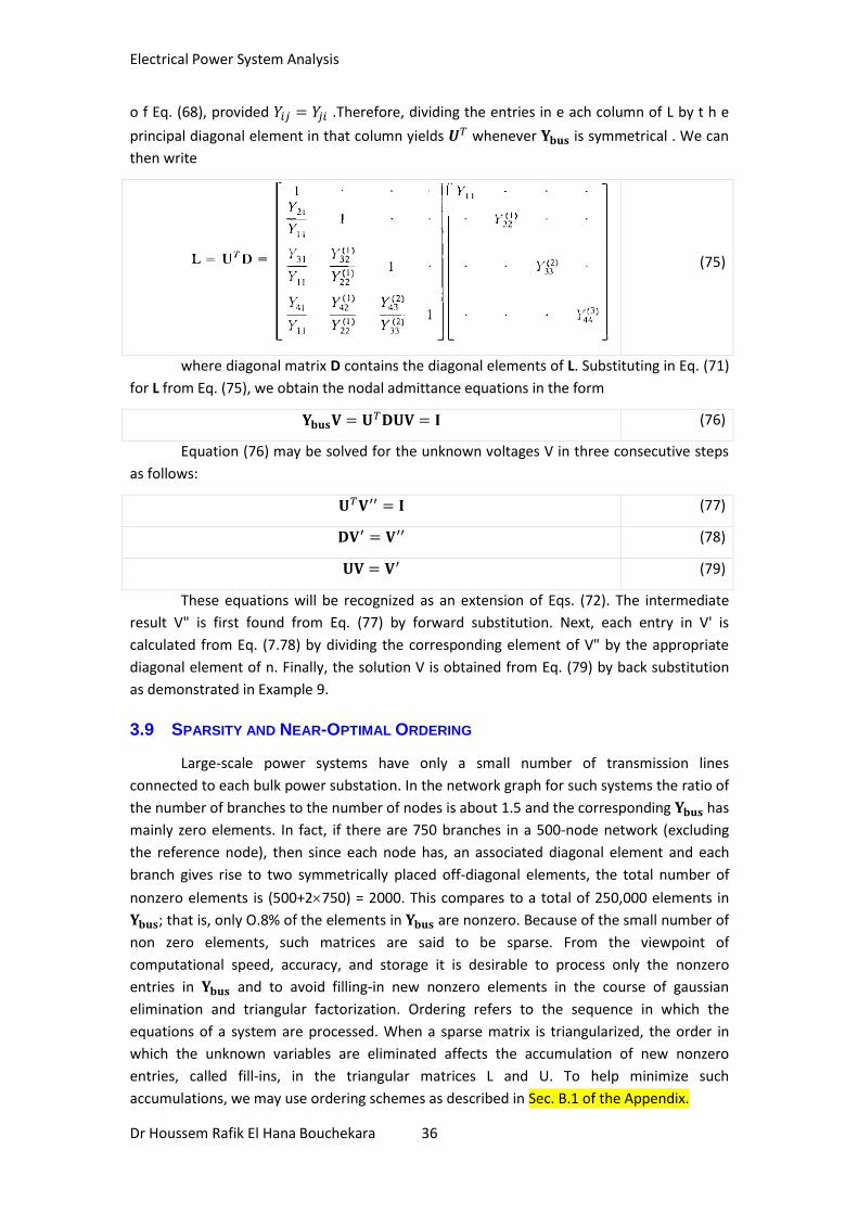
o f Eq. (68), provided .Therefore, dividing the entries in e ach column of L by t h e

principal diagonal element in that column yields whenever is symmetrical . We can

then write

(75)

where diagonal matrix D contains the diagonal elements of L. Substituting in Eq. (71)

for L from Eq. (75), we obtain the nodal admittance equations in the form

(76)

Equation (76) may be solved for the unknown voltages V in three consecutive steps

as follows:

(77)

(78)

(79)

These equations will be recognized as an extension of Eqs. (72). The intermediate

result V" is first found from Eq. (77) by forward substitution. Next, each entry in V' is

calculated from Eq. (7.78) by dividing the corresponding element of V" by the appropriate

diagonal element of n. Finally, the solution V is obtained from Eq. (79) by back substitution

as demonstrated in Example 9.

3.9 SPARSITY AND NEAR-OPTIMAL ORDERING

Large-scale power systems have only a small number of transmission lines

connected to each bulk power substation. In the network graph for such systems the ratio of

the number of branches to the number of nodes is about 1.5 and the corresponding has

mainly zero elements. In fact, if there are 750 branches in a 500-node network (excluding

the reference node), then since each node has, an associated diagonal element and each

branch gives rise to two symmetrically placed off-diagonal elements, the total number of

nonzero elements is (500+2750) = 2000. This compares to a total of 250,000 elements in

; that is, only O.8% of the elements in are nonzero. Because of the small number of

non zero elements, such matrices are said to be sparse. From the viewpoint of

computational speed, accuracy, and storage it is desirable to process only the nonzero

entries in and to avoid filling-in new nonzero elements in the course of gaussian

elimination and triangular factorization. Ordering refers to the sequence in which the

equations of a system are processed. When a sparse matrix is triangularized, the order in

which the unknown variables are eliminated affects the accumulation of new nonzero

entries, called fill-ins, in the triangular matrices L and U. To help minimize such

accumulations, we may use ordering schemes as described in Sec. B.1 of the Appendix.



3.10 SUMMARY

Nodal representation of the power transmission network is developed in this

chapter. The essential background for understanding the bus admittance matrix and its

formation is provided. Incorporation of mutually coupled branches into can be handled

by the building-block approach described here. Modifications to to reflect network

changes arc thereby facilitated.

Gaussian elimination offers an alternative to matrix inversion for solving large-scale

power systems, and triangular factorization of enhances computational efficiency and

reduces computer memory requirements, especially when the network matrices are

symmetric.

These modeling and numerical procedures underlie .the solution approaches now

being used in daily practice by the electric power industry for power-flow and system

analysis.

3.11 PROBLEMS

Problem 1

Form the for the network shown in Figure 18 including the generator buses.

Figure 18

Solution:

Problem 2

For the system shown in figure obtain by inspection method. Take bus (1) as

reference. The impedance marked are in p.u.



Figure 19

Solution:

Problem 3:

A power system consists of 4 buses. Generators are connected at buses 1 and 3

reactances of which are j0.2 and j0.l respectively. The transmission lines are connected

between buses 1-2, 1-4, 2-3 and 3-4 and have reactances j0.25, j0.5, j0.4 and j0.1

respectively. Find the bus admittance matrix (i) by direct inspection (ii) using bus incidence

matrix and admittance matrix.

Figure 20

Solution:



Problem 4

For the circuit shown in Figure 21, convert the voltage sources to equivalent current sources

and write nodal equations in matrix format using bus 0 as the reference bus.

Figure 21

Problem 5

Determine the 44 bus admittance matrix and write nodal equations in matrix

format for the circuit shown in Figure 22. Do not solve the equations.

Figure 22

Problem 6

Given the impedance diagram of a simple system as shown in Figure 2.31, draw the

admittance diagram for the system and develop the 4 4 bus admittance matrix by

inspection.



Figure 23

Solution:

Figure 24



Documents

Electrical Power System Analysis 3. the Admittance Model and Network