Electrical Power and Energy Systems 55 (2014) 1–12

Contents lists available at ScienceDirect

Electrical Power and Energy Systems

journal homepage: www.elsevier .com/locate / i jepes

Optimizing reactive power flow of HVDC systems using geneticalgorithm

0142-0615/$ - see front matter � 2013 Elsevier Ltd. All rights reserved.http://dx.doi.org/10.1016/j.ijepes.2013.08.006

⇑ Corresponding author. Address: Department of Mechatronics Engineering, CelalBayar Universirty, Manisa, Turkey. Tel./fax: +90 236 314 10 10

E-mail addresses: ulas.kilic@cbu.edu.tr (U. Kılıç), kayan@sakarya.edu.tr(K. Ayan), arifoglu@sakarya.edu.tr (U. Arifoglu).

Ulas� Kılıç a,⇑, Kürs�at Ayan b, Ugur Arifoglu c

a Department of Mechatronics Engineering, Celal Bayar Universirty, Manisa, Turkeyb Department of Computer Engineering, Sakarya University, Sakarya, Turkeyc Department of Electrical-Electronics Engineering, Sakarya University, Sakarya, Turkey

a r t i c l e i n f o

Article history:Received 2 August 2012Received in revised form 16 July 2013Accepted 8 August 2013

Keywords:Optimal reactive power flowIntegrated AC–DC systemHeuristic methodGenetic algorithmEvolutionary

a b s t r a c t

Due to the usage of high voltage direct current (HVDC) transmission links extensively in recent years, itrequires more studies in this issue. Two-terminal HVDC transmission link is one of most important ele-ments in electrical power systems. Generally, the representation of HVDC link is simplified for optimalreactive power flow (ORPF) studies in power systems. ORPF problem of purely AC power systems isdefined as minimization of power loss under equality and inequality constraints. Hence, ORPF problemof integrated AC–DC power systems is extended to incorporate HVDC links taking into considerationpower transfer control characteristics. In this paper, this problem is solved by genetic algorithm (GA) thatis an evolutionary-based heuristic algorithm for the first time. The proposed method is tested on themodified IEEE 14-bus test system, the modified IEEE 30-bus test system, and the modified New England39-bus test system. The validity, the efficiency, and effectiveness of the proposed method are shown bycomparing the obtained results with that reported in literature. Thus, the impact of DC transmission linkson the whole power systems is shown.

� 2013 Elsevier Ltd. All rights reserved.

1. Introduction

ORPF is an energy system problem that the scientists try tosolve for a long time [1–5]. The problem is minimization of thepower loss in an energy network. In other words, the aim is mini-mization of objective function which is power loss in an energysystem. At the same time, the objective function of whole systemis minimized under equality and inequality constraints. The equal-ity and inequality constraints in purely AC system are powerequalities defined for all the buses and physical constraints ofthe energy system, respectively. All the constraints have been tobe satisfied while the power loss of whole the system is beingminimized.

The scientists have used many different methods for solvingORPF problem of purely AC power systems [1–13]. These methodsare numerical and heuristic methods. According to the results re-ported in literature, it can be seen that heuristic methods are supe-rior from the numerical methods [4–13]. One important advantageof heuristic methods is that they convergence to the optimumsolution in shorter time than others and without reaching localminimums.

Because of the energy consumption increasing rapidly in recentyears, it is required to increase the power generation capacity. Thiscauses to over load the transmission lines. Thus, even small pertur-bations can cause a part of the energy system to leave the synchro-nization even if it is subjected to the small perturbations. It isneeded to reschedule energy systems to avoid such undesirable sit-uations like these and to maintain the continuity of the operating.So in recent years, the power system planners try to reschedule theenergy systems to transfer the power through HVDC links in recentyears. There are many advantages of the power transmissionthrough HVDC links. For examples, reactive power is not trans-ferred through HVDC links and energy loss of HVDC links is lesserthan long AC system transmission lines. Additionally, the instanta-neous power in neighboring AC systems can be controlled by HVDClinks. Furthermore, HVDC links is used to stabilize electric powersystems [14]. Recently, many researches are performed on realiza-tion of HVDC models for power flows studies [15–19]. The formu-lation for the basic model of two-terminal HVDC link is given inRef. [20].

In ORPF problem of the integrated AC–DC power systems, DClink constraints are included in the problem. In the literature, thereare two basic approaches for solving the power flow equations. Thefirst is the sequential approach [19,21,22]. In this method, AC andDC equations are solved separately by successive iterations.Although the implementation of the sequential method is simple,it has convergence problems associated with certain situations.

2 U. Kılıç et al. / Electrical Power and Energy Systems 55 (2014) 1–12

Furthermore the state vector does not contain explicitly DC vari-ables. The second approach is known as the unified approach[23]. In this study, the first method is used.

GA is a heuristic algorithm based on native selection. The basiclogic of this algorithm is based on the living of strong individuals innature and the dying of others. This algorithm consists of stages asinitial population, fitness scaling, selection, crossover, mutationand stopping. GA has been used successfully for solution of theengineering problem for a long time [24–29]. In this paper, GA isused for solution of ORPF problem in integrated AC–DC power sys-tems for the first time.

After this introduction, the modeling of DC transmission link isrepresented in Section 2. The methodology of GA is explained inSection 3. GA based optimal reactive power flow solution of HVDCsystems is explained in Section 4. In order to demonstrate validity,efficiency and effectiveness of the proposed method, simulation re-sults of the modified IEEE 14-bus test system, the modified IEEE30-bus test system and the modified New England 39-bus test sys-tem are given and the obtained results are extensively evaluatedand compared to that reported in the literature in section 5. Finally,the conclusions are discussed in section 6.

2. The modeling of DC transmission link

Before analyzing DC transmission system, it is necessary tomodel DC transmission link and the converters. The modeling ismade based on accepted assumptions in the literature. Theassumptions are as follows [23]:

� The main harmonic values of current and voltage in AC systemis balanced.� The other harmonics except the main harmonic are ignored.� The ripples in the form of DC current and voltages are ignored.� The thyristors used in the converters are accepted as ideal

switch and it is supposed to be short circuit in the direction oftransmission and open circuit in the direction of plugging.� No load current of the converter transformers and the losses are

ignored.

An AC bus having generators, AC lines, shunt compensators andconverters is represented in Fig. 1[30]. The active and reactivepower equalities at such a bus are given by Eqs. (1) and (2).

pgk ¼ plk þ pdk þ pk ð1Þ

qgk þ qsk ¼ qlk þ qdk þ qk ð2Þ

where pgk is the active power generation of the kth bus; plk the ac-tive load of the kth bus; pdk the active power transferred to dc line

Fig. 1. The representation of the ac bus whic

from the kth bus; pk the active power transferred to ac line from thekth bus; qgk the reactive power generation of the kth bus; qlk thereactive load of the kth bus; qdk the reactive power absorbed bythe converter in the kth bus; qk the reactive power transferred toac line from the kth bus; qsk the shunt compensator in the kth bus.

For rectifier bus,

pdk ¼ pr ð3Þ

qdk ¼ qr ð4Þ

For inverter bus,

pdk ¼ �pi ð5Þ

qdk ¼ qi ð6Þ

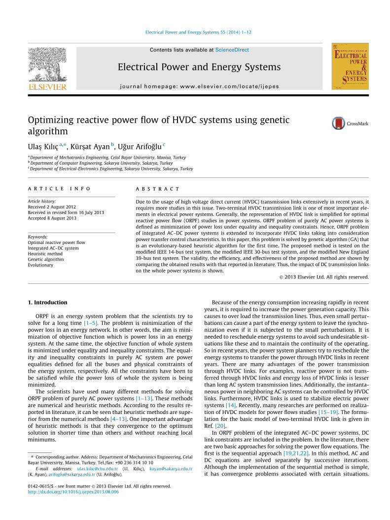
A basic schematic diagram of a two-terminal HVDC transmissionlink interconnecting buses ‘‘r’’ (rectifier) and ‘‘i’’ (inverter) is illus-trated in Fig. 2. The basic converter equations describing the rela-tionship between AC and DC variables were expressed in Ref. [31].

The variables shown in Fig. 2 are defined as follows:

vr is the primary line-to-line ac voltage (rms) of the rectifierside.Vi the primary line-to-line ac voltage (rms) of the inverter side.ur the phase angle of the rectifier side.ui the phase angle of the inverter side.ir ac current of the rectifier side.ii ac current of the inverter side.vdr the rectifier side voltage of DC link.vdi the inverter side voltage of DC link.id the direct current.t the transformer tap ratio.

2.1. The equations for rectifier side of DC transmission link

The equations related to the rectifier operation of a convertercan be expressed as follows:

mdor ¼ ktrmr ð7Þ

mdr ¼ mdor cos a� rcrid ð8Þ

where vdor is the ideal no-load direct voltage, k ¼ 3ffiffiffi2p

=p and a isthe ignition delay angle; rcr the so called equivalent commutatingresistance, which accounts for the voltage drop due to commutationoverlap and is proportional to the commutation reactance,rcr ¼

ffiffiffi3p

xcr=p. The active power for the rectifier side is determinedby:

pr ¼ mdrid ð9Þ

h is connected dc transmission link [30].

Fig. 2. A basic schematic diagram of a two-terminal HVDC transmission link [31].

Fig. 3. The equivalent circuit of a two-terminal HVDC link [32].

Fig. 4. The simple flow scheme of GA [35].

Table 1Cases with respect to the population sizes.

Cases 1 2 3 4 5

Initial population 10 20 30 40 50Crossover 5 10 15 20 25Mutation 1 2 3 4 5Cases 6 7 8 9 10Initial population 60 70 80 90 100Crossover 30 35 40 45 50Mutation 6 7 8 9 10

U. Kılıç et al. / Electrical Power and Energy Systems 55 (2014) 1–12 3

Since losses at the converter and transformer can be ignored (pr =pac), the reactive power at the rectifier side is determined asfollows:

qr ¼ prtan/rj j ð10Þ

where /r is the phase angle between the AC voltage and the funda-mental AC current and is calculated by neglecting the commutationoverlap as follows:

/r ¼ cos�1ðmdr=mdorÞ ð11Þ

The equivalent circuit of a two-terminal HVDC link is shown inFig. 3[32] and the related relationships are given by Eqs. (8), (13),and (17).

2.2. The equations for inverter side of DC transmission link

The equations related to the inverter operation of a convertercan be expressed as follows:

mdoi ¼ ktimi ð12Þ

mdi ¼ mdoi cos c� rciid ð13Þ

pi ¼ mdiid ð14Þ

qi ¼ pitan/ij j ð15Þ

/i ¼ cos�1ðmdi=mdoiÞ ð16Þ

where c is the extinction advance angle.

2.3. DC link equation

The relationship between the voltages of both sides of DC linkvoltages can be expressed by Eq. (17):

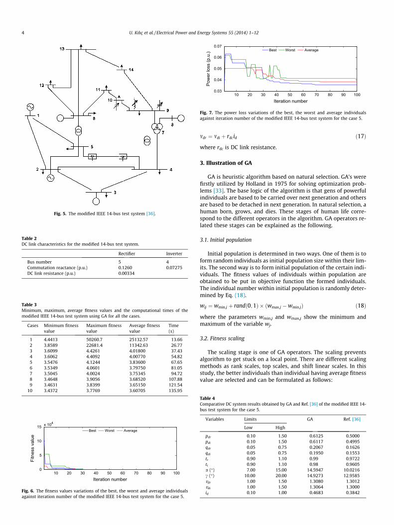
Fig. 5. The modified IEEE 14-bus test system [36].

Table 2DC link characteristics for the modified 14-bus test system.

Rectifier Inverter

Bus number 5 4Commutation reactance (p.u.) 0.1260 0.07275DC link resistance (p.u.) 0.00334

Table 3Minimum, maximum, average fitness values and the computational times of themodified IEEE 14-bus test system using GA for all the cases.

Cases Minimum fitnessvalue

Maximum fitnessvalue

Average fitnessvalue

Time(s)

1 4.4413 50260.7 25132.57 13.662 3.8589 22681.4 11342.63 26.773 3.6099 4.4261 4.01800 37.434 3.6062 4.4092 4.00770 54.825 3.5476 4.1244 3.83600 67.656 3.5349 4.0601 3.79750 81.057 3.5045 4.0024 3.75345 94.728 3.4648 3.9056 3.68520 107.889 3.4631 3.8399 3.65150 121.54

10 3.4372 3.7769 3.60705 135.95

10 20 30 40 50 60 70 80 90 1000

5

10

15 x 104

Iteration number

Fitn

ess

valu

e

Best Worst Average

Fig. 6. The fitness values variations of the best, the worst and average individualsagainst iteration number of the modified IEEE 14-bus test system for the case 5.

10 20 30 40 50 60 70 80 90 1000.03

0.04

0.05

0.06

0.07

Iteration number

Pow

er lo

ss (p

.u.) Best Worst Average

Fig. 7. The power loss variations of the best, the worst and average individualsagainst iteration number of the modified IEEE 14-bus test system for the case 5.

4 U. Kılıç et al. / Electrical Power and Energy Systems 55 (2014) 1–12

mdr ¼ mdi þ rdcid ð17Þ

where rdc is DC link resistance.

3. Illustration of GA

GA is heuristic algorithm based on natural selection. GA’s werefirstly utilized by Holland in 1975 for solving optimization prob-lems [33]. The base logic of the algorithm is that gens of powerfulindividuals are based to be carried over next generation and othersare based to be detached in next generation. In natural selection, ahuman born, grows, and dies. These stages of human life corre-spond to the different operators in the algorithm. GA operators re-lated these stages can be explained as the following.

3.1. Initial population

Initial population is determined in two ways. One of them is toform random individuals as initial population size within their lim-its. The second way is to form initial population of the certain indi-viduals. The fitness values of individuals within population areobtained to be put in objective function the formed individuals.The individual number within initial population is randomly deter-mined by Eq. (18).

wij ¼ wmin;j þ randð0;1Þ � ðwmax;j �wmin;jÞ ð18Þ

where the parameters wmin,j and wmax,j show the minimum andmaximum of the variable wj.

3.2. Fitness scaling

The scaling stage is one of GA operators. The scaling preventsalgorithm to get stuck on a local point. There are different scalingmethods as rank scales, top scales, and shift linear scales. In thisstudy, the better individuals than individual having average fitnessvalue are selected and can be formulated as follows:

Table 4Comparative DC system results obtained by GA and Ref. [36] of the modified IEEE 14-bus test system for the case 5.

Variables Limits GA Ref. [36]

Low High

pdr 0.10 1.50 0.6125 0.5000pdi 0.10 1.50 0.6117 0.4995qdr 0.05 0.75 0.2067 0.1626qdi 0.05 0.75 0.1950 0.1553tr 0.90 1.10 0.99 0.9722ti 0.90 1.10 0.98 0.9605a (�) 7.00 15.00 14.5947 10.0216c (�) 10.00 20.00 14.9273 12.9585vdr 1.00 1.50 1.3080 1.3012vdi 1.00 1.50 1.3064 1.3000id 0.10 1.00 0.4683 0.3842

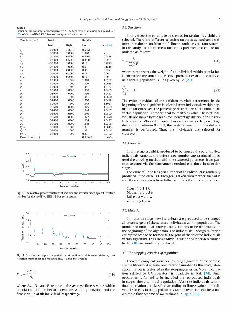
Table 5Limits on the variables and comparative AC system results obtained by GA and Ref.[36] of the modified IEEE 14-bus test system for the case 5.

Variables (p.u.) Limits Results

Low High GA Ref. [36]

pg1 0.0000 3.3240 0.5458 –pg2 0.0000 2.0000 1.0803 –qg1 �0.1000 0.5000 0.0003 �0.0838qg2 �0.1000 0.5000 0.0548 �0.0981qc3 �0.1000 1.0000 0.17 0.2873qc6 �0.1000 1.0000 0.51 0.1815qc8 �0.1000 0.8000 0.09 0.327qc9 0.0000 0.2000 0.18 0.00qc10 0.0000 0.2000 0.10 0.00v1 1.0000 1.1500 1.060 1.0707v2 1.0000 1.1500 1.056 1.0618v3 1.0000 1.1500 1.041 1.0747v4 0.9500 1.0500 1.036 1.0495v5 0.9500 1.0500 1.036 1.0422v6 1.0000 1.1500 1.041 1.0620v7 0.9500 1.0500 1.030 1.0498v8 1.0000 1.1500 1.045 1.1021v9 0.9500 1.0500 1.045 1.0499v10 0.9500 1.0500 1.044 1.0447v11 0.9500 1.0500 1.040 1.0500v12 0.9500 1.0500 1.027 1.0470v13 0.9500 1.0500 1.024 1.0427v14 0.9500 1.0500 1.018 1.0286t(5–6) 0.9000 1.1000 1.07 1.0015t(4–7) 0.9000 1.1000 1.05 1.0546t(4–9) 0.9000 1.1000 0.93 0.9162Power loss (p.u.) 0.035476 0.0425

10 20 30 40 50 60 70 80 90 1000.1

0.2

0.3

0.4

0.5

Iteration number

Q (p

.u.)

Qr Qi

Fig. 8. The reactive power variations at rectifier and inverter sides against iterationnumber for the modified IEEE 14-bus test system.

10 20 30 40 50 60 70 80 90 1000.9

1

1.1

1.2

1.3

Iteration number

Tran

sfor

mer

tap

ratio tr ti

Fig. 9. Transformer tap ratio variations at rectifier and inverter sides againstiteration number for the modified IEEE 14-bus test system.

U. Kılıç et al. / Electrical Power and Energy Systems 55 (2014) 1–12 5

Fave ¼PNk

i¼1Fi

Nkð19Þ

where Fave, Nk, and Fi represent the average fitness value withinpopulation, the number of individuals within population, and thefitness value of ith individual, respectively.

3.3. Selection

In this stage, the parents to be crossed for producing a child areselected. There are different selection methods as stochastic uni-form, remainder, uniform, shift linear, roulette and tournament.In this study, the tournament method is preferred and can be for-mulated as follows:

si ¼FiPNkj¼1Fj

ð20Þ

where si represents the weight of ith individual within population.Furthermore, the sum of the elective probabilities of all the individ-uals within population is 1 as given by Eq. (21).

XNk

i¼1

si ¼ 1 ð21Þ

The twice individual of the children number determined in thebeginning of the algorithm is selected from individuals within pop-ulation for crossover. The percentage distribution of the individualswithin population is proportional to its fitness value. The best indi-viduals are shown by the high-level percentage distributions in rou-lette selection. After all the individuals are shown as the percentagedistribution between 0 and 1, the roulette selection in the definitenumber is performed. Thus, the individuals are selected forcrossover.

3.4. Crossover

In this stage, a child is produced to be crossed the parents. Newindividuals same as the determined number are produced to beused the crossing method with the scattered parameter from par-ents selected via the tournament method explained in selectionstage.

The value of 1 and 0 as gen number of an individual is randomlyproduced. If the value is 1, then gen is taken from mother, the valueis 0, then gen is taken from father and thus the child is produced.

Cross: 1 0 1 1 0Mother: a b c d eFather: x y z u wChild: a y c d w

3.5. Mutation

In mutation stage, new individuals are produced to be changedall or some gens of the selected individuals within population. Thenumber of individual undergo mutation has to be determined inthe beginning of the algorithm. The individuals undergo mutationare reproduced to be formed all the gens of the selected individualswithin algorithm. Thus, new individuals as the number determinedby Eq. (18) are randomly produced.

3.6. The stopping criterion of algorithm

There are many criterions for stopping algorithm. Some of theseare the fitness value, time, and iteration number. In this study, iter-ation number is preferred as the stopping criterion. More informa-tion related to GA operators is available in Ref. [34]. Finalpopulation is formed to be included the reproduced individualsin stages above to initial population. After the individuals withinfinal population are classified according to fitness value, the indi-vidual same as initial population is carried over the next iteration.A simple flow scheme of GA is shown in Fig. 4 [35].

1

G G

2 3 4

14

12

13

C

15

23

18

19 20

2425 26

1617

10

21

C

293027 28

C

811

6

7

C

5

Case A

Case B

22

G Generators

C Synchronous condensors

Fig. 10. The modified IEEE 30-bus system [37].

Table 6Minimum, maximum and average fitness values and the computational times of themodified IEEE 30-bus test system using GA for all the cases.

Cases Case A Case B Time (s)

Min. Max. Min. Max.

1 13.1991 9638.4 13.8739 98282 14.892 12.7144 8267.8 13.8671 48105 29.823 12.5840 1016.29 12.2364 34138 46.234 12.4832 197.680 12.1307 11216 62.405 12.4065 14.2020 12.0150 13.5989 74.866 12.1908 13.4281 11.6110 12.2419 89.477 12.1855 13.0647 11.5668 12.1656 107.848 11.9083 12.7198 11.5198 12.1189 119.859 11.7488 12.5078 11.4933 12.0325 134.50

10 11.7081 12.1332 11.4872 11.8849 153.78

10 20 30 40 50 60 70 80 90 1000

1

2

3

4 x 104

Iteration number

Fitn

ess

valu

e Best Worst Average

Fig. 11. For Case A, the fitness value variations of the best, the worst and averageindividuals against iteration number of the modified IEEE 30-bus test system for thecase 5.

10 20 30 40 50 60 70 80 90 1000

0.5

1

1.5

2 x 105

Iteration number

Fitn

ess

valu

e Best Worst Average

Fig. 12. For Case B, the fitness value variations of the best, the worst and averageindividuals against iteration number of the modified IEEE 30-bus test system for thecase 5.

10 20 30 40 50 60 70 80 90 1000.1

0.15

0.2

0.25

Iteration number

Pow

er lo

ss (p

.u.) Best Worst Average

Fig. 13. For Case A, the power loss variations of the best, the worst and averageindividuals against iteration number of the modified IEEE 30-bus test system for thecase 5.

6 U. Kılıç et al. / Electrical Power and Energy Systems 55 (2014) 1–12

4. Optimizing reactive power flow of HVDC systems using GA

In order to solve ORPF problem of HVDC systems, we have todetermine the control and the variables. The control variables

10 20 30 40 50 60 70 80 90 1000.1

0.15

0.2

0.25

0.3

Iteration number

Pow

er lo

ss (p

.u.) Best Worst Average

Fig. 14. For Case B, the power loss variations of the best, the worst and averageindividuals against iteration number of the modified IEEE 30-bus test system for thecase 5.

Table 7Comparative DC system results obtained by GA and Ref. [37].

Variables Limits Case A Case B

Low High GA Ref. [37] GA Ref. [37]

pdr 0.10 1.50 0.2749 0.2502 0.2749 0.2503pdi 0.10 1.50 0.2719 – 0.2720 –qdr 0.05 0.75 0.0641 0.1000 0.0752 0.1002qdi 0.05 0.75 0.0664 – 0.0614 –tr 1.00 1.10 1.00 1.0020 1.02 1.025ti 1.00 1.10 1.00 1.0034 1.00 1.020a (�) 9.74 22.91 12.5255 22.5630 14.9068 22.9125c (�) 8.59 22.91 13.8534 14.6276 12.1654 22.6833vdr 1.00 1.50 1.3786 – 1.3800 –vdi 1.00 1.50 1.3636 – 1.3651 –id 0.10 1.00 0.1994 0.1007 0.1992 0.3000

Table 8Limits on the variables and comparative AC system results obtained by GA and Ref.[37] of the modified IEEE 30-bus test system for the case 5.

Variables (p.u.) Limits Case A Case B

Low High GA Ref. [37] GA Ref. [37]

pg1 0.00 3.602 1.6057 – 1.5897 –pg2 0.00 1.40 1.3552 – 1.3673 –qg1 �1.00 1.00 0.2951 �0.7280 0.1921 0.4065qg2 �0.40 0.50 0.2605 0.4890 0.2027 0.3101qc5 �0.40 0.40 0.34 0.3882 0.39 0.0362qc8 �0.10 0.40 0.32 0.3988 0.32 0.3343qc11 �0.06 0.24 0.08 0.2351 0.19 0.2311qc13 �0.06 0.24 0.23 0.1438 0.23 0.0865v1 1.00 1.15 1.075 1.1114 1.063 1.0994v2 1.00 1.15 1.050 1.0883 1.041 1.0867v3 0.90 1.05 1.026 – 1.021 –v4 0.90 1.05 1.014 – 1.010 –v5 1.00 1.15 1.007 1.0708 1.006 1.0754v6 0.90 1.05 1.003 – 1.002 –v7 0.90 1.05 0.997 – 0.996 –v8 1.00 1.15 1.001 1.0585 1.000 1.0679v9 0.90 1.05 1.049 – 1.047 –v10 0.90 1.05 1.019 – 1.031 –v11 1.00 1.15 1.064 1.1159 1.084 1.1064v12 0.90 1.05 1.047 – 1.049 –v13 1.00 1.15 1.077 1.0555 1.079 1.0211v14 0.90 1.05 1.044 – 1.033 –v15 0.90 1.05 1.024 – 1.028 –v16 0.90 1.05 1.027 – 1.038 –v17 0.90 1.05 1.017 – 1.028 –v18 0.90 1.05 1.010 – 1.017 –v19 0.90 1.05 1.004 – 1.013 –v20 0.90 1.05 1.007 – 1.017 –v21 0.90 1.05 1.007 – 1.018 –v22 0.90 1.05 1.008 – 1.019 –v23 0.90 1.05 1.010 – 1.016 –v24 0.90 1.05 1.000 – 1.009 –v25 0.90 1.05 1.010 1.0049 1.020 0.9935v26 0.90 1.05 0.992 0.9823 1.002 0.9716v27 0.90 1.05 1.025 1.0129 1.035 0.9940v28 0.90 1.05 0.997 – 0.996 –v29 0.90 1.05 1.005 0.9676 1.015 0.9502v30 0.90 1.05 0.994 0.9714 1.004 0.9547t(6–9) 0.90 1.10 0.92 1.0269 0.96 1.0001t(6–10) 0.90 1.10 1.01 1.0000 0.93 1.0000t(4–12) 0.90 1.10 0.95 1.0000 0.95 1.0001t(28–27) 0.90 1.10 0.94 1.0010 0.93 1.0380Power loss (p.u.) 0.1240 0.2841 0.1201 0.2811

10 20 30 40 50 60 70 80 90 1000.05

0.1

0.15

0.2

Iteration number

Q (p

.u.)

Qr Qi

Fig. 15. For Case A, the reactive power variations at rectifier and inverter sidesagainst iteration number for the modified IEEE 30-bus test system.

U. Kılıç et al. / Electrical Power and Energy Systems 55 (2014) 1–12 7

should be the same as those of the problem to be optimized. Thecontrol variables of the AC–DC system are:

u ¼ ½uAC ;uDC � ð22Þ

uAC ¼ ½pg2; . . . ;pgNg ; mg1; . . . ; mgNg ; qs1; . . . ; qsNs; t1; . . . ; tNT �: ð23Þ

uDC ¼ ½pr ;pi; qr ; qi; id� ð24Þ

where pgi except the slack unit pslack is the generator active poweroutputs, vgi the generator voltage, Ng the number of generatorbuses, Ns the number of shunt compensators and NT the numberof transformers, respectively.

The state variables of the AC–DC system are:

x ¼ ½xAC ; xDC � ð25Þ

xAC ¼ ½pgslack; qg1; . . . ; qgNg ; ml1; . . . ; mlNl� ð26Þ

xDC ¼ ½tr; ti;a; c; mdr ; mdi� ð27Þ

where pgslack is the slack bus active power output, qgi the reactivepower output, vli the load bus voltage, Nl the number of load buses,respectively.

For updating active and reactive power at rectifier and inverterbus, we use the following formulas:

For rectifier bus:

pupdateload ¼ pload þ pr

qupdateload ¼ qload þ qr

ð28Þ

For inverter bus:

pupdateload ¼ pload � pi

qupdateload ¼ qload þ qi

ð29Þ

The fitness value for each individual is obtained by Eq. (30) asfollows:

Fi ¼ K1pLoss þ K2jpslack � plimslackj þ K3

XNg

i¼1

jqgi � qlimgi j þ K4

XNl

i¼1

jmli

� mlimli j þ K5jtr � tlim

r j þ K6jti � tlimi j þ K7ja� alimj þ K8jc

� climj þ K9jmdr � mlimdr j þ K10jmdi � mlim

di j ð30Þ

where plimslack, qlim

gi , mlimli , tlim

r , tlimi , alim, clim, mlim

dr and mlimdi show the limits

of the related variables, respectively; K1, K2, K3, K4, K5, K6, K7, K8, K9,and K10 are penalty weights of power loss, real power output of

10 20 30 40 50 60 70 80 90 1000

0.05

0.1

0.15

0.2

Iteration number

Q (p

.u.)

Qr Qi

Fig. 16. For Case B, the reactive power variations at rectifier and inverter sidesagainst iteration number for the modified IEEE 30-bus test system.

10 20 30 40 50 60 70 80 90 1000.98

1.02

1.06

1.1

1.14

1.18

Iteration number

Tran

sfor

mer

tap

ratio tr ti

Fig. 17. For Case A, transformer tap ratio variations at rectifier and inverter sidesagainst iteration number for the modified IEEE 30-bus test system.

10 20 30 40 50 60 70 80 90 1000.98

1.02

1.06

1.1

1.14

Iteration number

Tran

sfor

mer

tap

ratio tr ti

Fig. 18. For Case B, transformer tap ratio variations at rectifier and inverter sidesagainst iteration number for the modified IEEE 30-bus test system.

8 U. Kılıç et al. / Electrical Power and Energy Systems 55 (2014) 1–12

slack bus, reactive power outputs of generator buses, load bus volt-age magnitudes, the effective transformer ratio’s of rectifier and in-verter sides, the angles of rectifier and inverter sides, the directvoltages of rectifier and inverter sides respectively. Note that thevalue of penalty function grows with a quadratic form when theconstraints are violated and is 0 in the region where constraintsare not violated.

The power flow calculation for each individual in heuristicmethods is performed and a fitness value Fi for each individual iscalculated to evaluate its quality as follows:

Step 1: Update pload and qload at rectifier and inverter sides byusing Eqs. (28) and (29)

Step 2: Run Newton-RaphsonStep 3: Calculate the values of tr, ti, a, c, vdr, vdi

Step 4: Calculate the fitness value Fi by using Eq. (30)

ploss ¼XNg

i¼1

pgi �XN

j¼1

plj ð31Þ

where ploss represents the real power transmission line losses, plj

represents the active load of jth bus.The flowchart of genetic algorithm is defined as follows:

Step 1. Read system data and GA parameters.Step 2. Generate initial population of n individuals via control

variable u.Step 3. Calculate the fitness value Fi of each chromosome in the

population.

Step 4. Create a new population by repeating the following stepsuntil the new population is completed.

Step 5. Select the parents by tournament selection.Step 6. Crossover the parent chromosomes to form a new child

with scattered.Step 7. Mutate new child with a mutation probability.Step 8. Calculate the fitness Fi of each new child.Step 9. Include new child to the population.Step 10. Classify the all individuals from minimum to maximum.Step 11. Carry over the individual same as initial population to

the next iteration.Step 12. If the stopping criterion is satisfied, stop algorithm and

show the best solution in current population else, go toStep 4..

5. Application of GA on test systems and the simulation results

In this study, the proposed method is applied to four differenttest systems those are the modified IEEE 14-bus test system, themodified IEEE 30-bus test system and the modified New England39-bus test system. The simulations are performed for differentpopulation sizes given in Table 1. For these systems, minimum,maximum, average fitness values and the computational times ob-tained by GA are given in the bottom. It can be seen from resultsthat the optimum solution is not obtained by increasing the popu-lation size and the computational times of the software increase asthe population size increases. The optimum solution is obtained bytrials. The crossover rate and the mutation rate inside of the algo-rithm are taken into account as a constant such as the populationcan be compared to other studies. These values are 50% and 10%,respectively. Furthermore, the results obtained by the proposedmethod are compared to those reported in literature. The proposedalgorithm is run on a computer with I3 CPU 2.4 GHz, 2 GB RAM. Inorder to test the validity, the effectiveness, and the efficiency of theproposed method, the test systems mentioned above are used. Thealgorithm proposed in this study is developed via real GA codeswithout using GA tool on Matlab.

In this study, the transformer tap ratios and the switchableshunt capacitor/reactor banks are taken into consideration as dis-crete variables. The transformer tap-step and the bank/unit capac-ity-step are also selected as being 0.01 p.u.

5.1. The modified IEEE 14-bus test system

The modified IEEE 14-bus test system is shown in Fig. 5[36]. Atwo-terminal HVDC link is included to between buses 4 and 5 inthe original IEEE 14-bus test system. This system has 20 ac trans-mission lines, 2 generators, 3 transformers, 3 synchronous con-densers and 2 switchable VAR compensators. The bus 4 isselected as rectifier and then the bus 5 is selected as inverter bus.

The characteristics of DC transmission link are given in Table 2.For all the cases, minimum, maximum, average fitness values

and the computational times obtained by GA for the modified IEEE14-bus test system are given Table 3. Although the computationaltimes of the software are very low for the population sizes in cases1, and 2 minimum, maximum and average fitness values are somuch and the variables exceed their limits. The variables do notexceed their limits for the population sizes in cases 3–10. For thesecases, it can be seen from Table 3 that the computational times in-crease considerably, as the average fitness values decrease fromcase 3 to case 10. In order to show the superiority of the proposedmethod, the population size which obtains better than solution re-ported in literature is determined as best one. Therefore optimumpopulation size for this test system is taken into account as case 5.

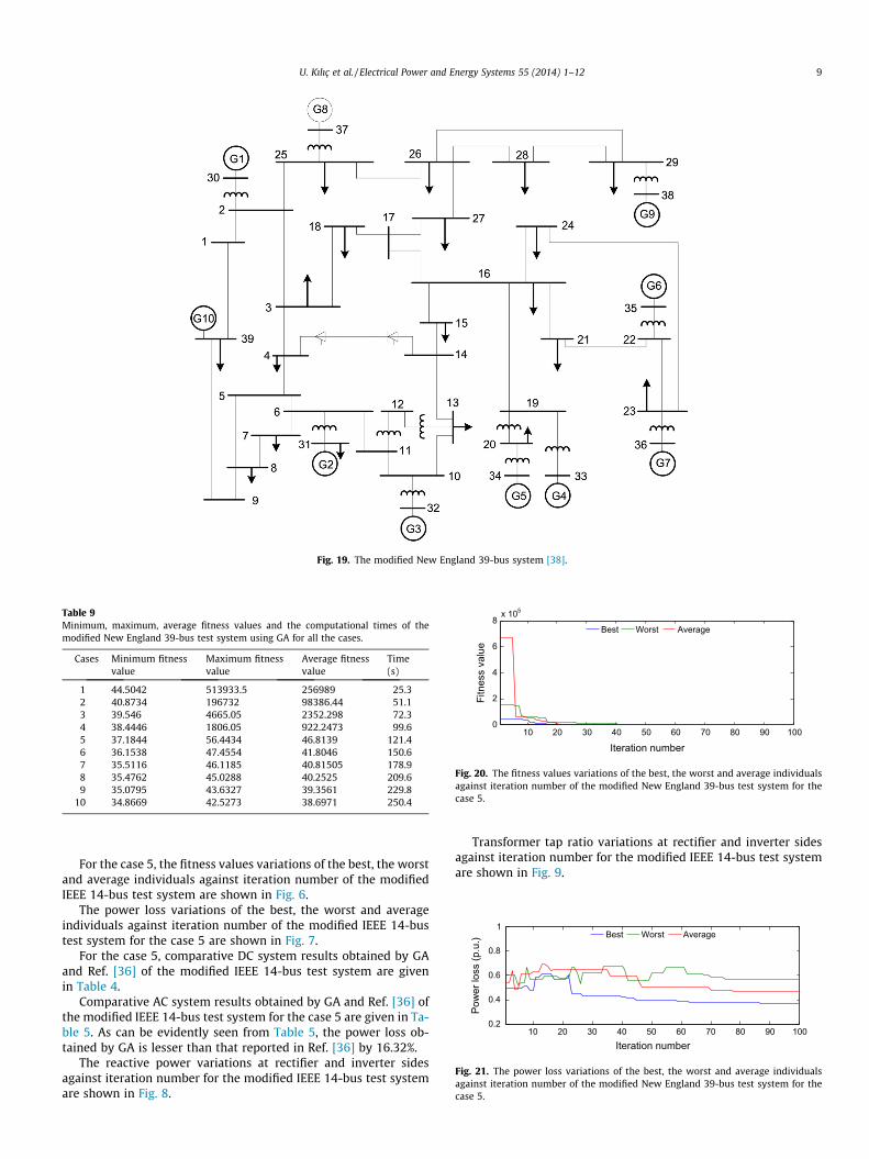
Fig. 19. The modified New England 39-bus system [38].

Table 9Minimum, maximum, average fitness values and the computational times of themodified New England 39-bus test system using GA for all the cases.

Cases Minimum fitnessvalue

Maximum fitnessvalue

Average fitnessvalue

Time(s)

1 44.5042 513933.5 256989 25.32 40.8734 196732 98386.44 51.13 39.546 4665.05 2352.298 72.34 38.4446 1806.05 922.2473 99.65 37.1844 56.4434 46.8139 121.46 36.1538 47.4554 41.8046 150.67 35.5116 46.1185 40.81505 178.98 35.4762 45.0288 40.2525 209.69 35.0795 43.6327 39.3561 229.8

10 34.8669 42.5273 38.6971 250.4

10 20 30 40 50 60 70 80 90 1000

2

4

6

8x 105

Iteration number

Fitn

ess

valu

e

Best Worst Average

Fig. 20. The fitness values variations of the best, the worst and average individualsagainst iteration number of the modified New England 39-bus test system for thecase 5.

10 20 30 40 50 60 70 80 90 1000.2

0.4

0.6

0.8

1

Iteration number

Pow

er lo

ss (p

.u.) Best Worst Average

Fig. 21. The power loss variations of the best, the worst and average individualsagainst iteration number of the modified New England 39-bus test system for thecase 5.

U. Kılıç et al. / Electrical Power and Energy Systems 55 (2014) 1–12 9

For the case 5, the fitness values variations of the best, the worstand average individuals against iteration number of the modifiedIEEE 14-bus test system are shown in Fig. 6.

The power loss variations of the best, the worst and averageindividuals against iteration number of the modified IEEE 14-bustest system for the case 5 are shown in Fig. 7.

For the case 5, comparative DC system results obtained by GAand Ref. [36] of the modified IEEE 14-bus test system are givenin Table 4.

Comparative AC system results obtained by GA and Ref. [36] ofthe modified IEEE 14-bus test system for the case 5 are given in Ta-ble 5. As can be evidently seen from Table 5, the power loss ob-tained by GA is lesser than that reported in Ref. [36] by 16.32%.

The reactive power variations at rectifier and inverter sidesagainst iteration number for the modified IEEE 14-bus test systemare shown in Fig. 8.

Transformer tap ratio variations at rectifier and inverter sidesagainst iteration number for the modified IEEE 14-bus test systemare shown in Fig. 9.

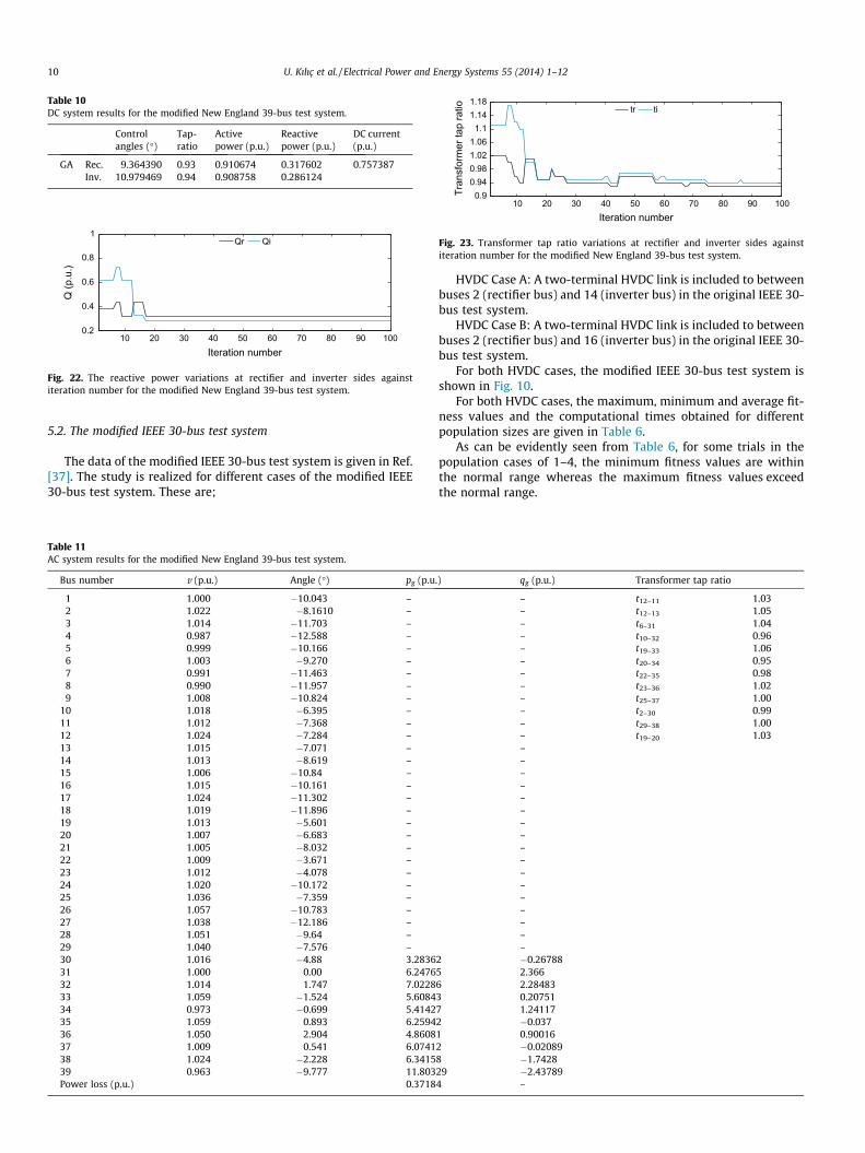
Table 10DC system results for the modified New England 39-bus test system.

Controlangles (�)

Tap-ratio

Activepower (p.u.)

Reactivepower (p.u.)

DC current(p.u.)

GA Rec. 9.364390 0.93 0.910674 0.317602 0.757387Inv. 10.979469 0.94 0.908758 0.286124

10 20 30 40 50 60 70 80 90 1000.2

0.4

0.6

0.8

1

Iteration number

Q (p

.u.)

Qr Qi

Fig. 22. The reactive power variations at rectifier and inverter sides againstiteration number for the modified New England 39-bus test system.

10 20 30 40 50 60 70 80 90 1000.9

0.940.981.021.061.1

1.141.18

Iteration number

Tran

sfor

mer

tap

ratio tr ti

Fig. 23. Transformer tap ratio variations at rectifier and inverter sides againstiteration number for the modified New England 39-bus test system.

10 U. Kılıç et al. / Electrical Power and Energy Systems 55 (2014) 1–12

5.2. The modified IEEE 30-bus test system

The data of the modified IEEE 30-bus test system is given in Ref.[37]. The study is realized for different cases of the modified IEEE30-bus test system. These are;

Table 11AC system results for the modified New England 39-bus test system.

Bus number v (p.u.) Angle (�) pg (p.u

1 1.000 �10.043 –2 1.022 �8.1610 –3 1.014 �11.703 –4 0.987 �12.588 –5 0.999 �10.166 –6 1.003 �9.270 –7 0.991 �11.463 –8 0.990 �11.957 –9 1.008 �10.824 –

10 1.018 �6.395 –11 1.012 �7.368 –12 1.024 �7.284 –13 1.015 �7.071 –14 1.013 �8.619 –15 1.006 �10.84 –16 1.015 �10.161 –17 1.024 �11.302 –18 1.019 �11.896 –19 1.013 �5.601 –20 1.007 �6.683 –21 1.005 �8.032 –22 1.009 �3.671 –23 1.012 �4.078 –24 1.020 �10.172 –25 1.036 �7.359 –26 1.057 �10.783 –27 1.038 �12.186 –28 1.051 �9.64 –29 1.040 �7.576 –30 1.016 �4.88 3.283631 1.000 0.00 6.247632 1.014 1.747 7.022833 1.059 �1.524 5.608434 0.973 �0.699 5.414235 1.059 0.893 6.259436 1.050 2.904 4.860837 1.009 0.541 6.074138 1.024 �2.228 6.341539 0.963 �9.777 11.803Power loss (p.u.) 0.3718

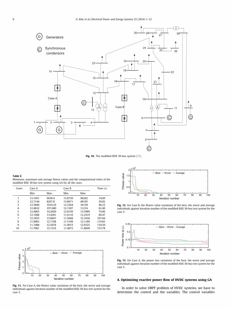
HVDC Case A: A two-terminal HVDC link is included to betweenbuses 2 (rectifier bus) and 14 (inverter bus) in the original IEEE 30-bus test system.

HVDC Case B: A two-terminal HVDC link is included to betweenbuses 2 (rectifier bus) and 16 (inverter bus) in the original IEEE 30-bus test system.

For both HVDC cases, the modified IEEE 30-bus test system isshown in Fig. 10.

For both HVDC cases, the maximum, minimum and average fit-ness values and the computational times obtained for differentpopulation sizes are given in Table 6.

As can be evidently seen from Table 6, for some trials in thepopulation cases of 1–4, the minimum fitness values are withinthe normal range whereas the maximum fitness values exceedthe normal range.

.) qg (p.u.) Transformer tap ratio

– t12–11 1.03– t12–13 1.05– t6–31 1.04– t10–32 0.96– t19–33 1.06– t20–34 0.95– t22–35 0.98– t23–36 1.02– t25–37 1.00– t2–30 0.99– t29–38 1.00– t19–20 1.03–––––––––––––––––

2 �0.267885 2.3666 2.284833 0.207517 1.241172 �0.0371 0.900162 �0.020898 �1.742829 �2.437894 –

U. Kılıç et al. / Electrical Power and Energy Systems 55 (2014) 1–12 11

The minimum and maximum fitness values are within the nor-mal range in the population cases of 5–10. Although the computa-tional time difference between population cases 5 and 10 is great,the fitness value difference between cases 5 and 10 is low. On thisaccount, acceptable population size is determined as case 5 forboth HVDC cases.

For both HVDC cases, the fitness value variations of the best, theworst and average individuals against iteration number are shownin Figs. 11 and 12, respectively.

For both HVDC cases, power loss variations of the best, theworst and average individuals against iteration number are shownin Figs. 13 and 14, respectively.

Comparative DC system results obtained by GA and Ref. [37] aregiven in Table 7.

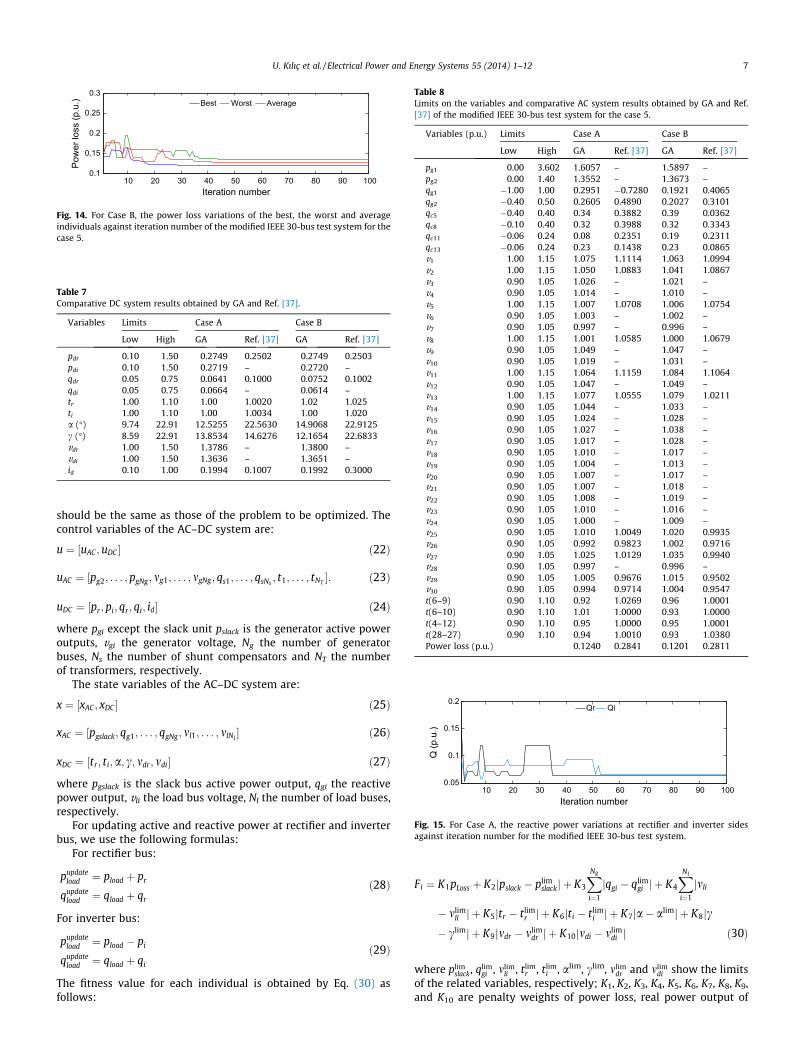
Comparative AC system results obtained by GA and Ref. [37] aregiven in Table 8. As can be evidently seen from Table 8, the powerlosses obtained by GA and the numerical method in Ref. [37] forHVDC Case A are 0.1240 and 0.2841, respectively. The power lossesobtained by GA and the numerical method in Ref. [37] for HVDCCase B are also 0.1201 and 0.2811, respectively. For both HVDCcases, the results obtained by GA are lesser than those reportedin Ref. [37] by 56.35% and 57.27%, respectively.

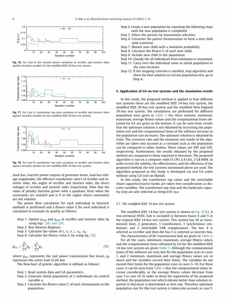
For both HVDC cases, the reactive power variations at rectifierand inverter sides against iteration number are shown in Figs. 15and 16, respectively.

For both HVDC cases, transformer tap ratio variations at recti-fier and inverter sides against iteration number are shown inFigs. 17 and 18, respectively.

For both HVDC cases, as can be evidently seen from Figs. 17 and18 that the transformer tap ratios are within limits at the end ofthe iteration.

5.3. The modified New England 39-bus test system

AC transmission line between buses 4 and 14 in the originalNew England 39-bus test system is replaced with a two terminalHVDC link and the modified New England 39-bus test systemshown in Fig. 19 is obtained [38]. The upper and lower limits ofthe transformer tap ratios in power system are 1.1 p.u. and 0.9p.u., respectively. DC link data for this test system is the same asthat of the modified 14 bus-test system.

The simulation results obtained by the trials are given inTable 9.

By reason of comparison of the fitness values and the computa-tional times, the optimum solution is determined as case 5. Forcase 5, the variations of the best, the worst, and the average fitnessvalues against iteration number is shown in Fig. 20.

The power loss variations of the best, the worst and averageindividuals against iteration number for case 5 of the modifiedNew England 39-bus test system are shown in Fig. 21.

AC and DC system variables obtained by the proposed algorithmare given in Tables 10 and 11, respectively.

The reactive power variations at rectifier and inverter sidesagainst iteration number for the modified New England 39-bus testsystem are shown in Fig. 22.

Transformer tap ratio variations at rectifier and inverter sidesagainst iteration number for the modified New England 39-bus testsystem are shown in Fig. 23.

6. Conclusion and discussion

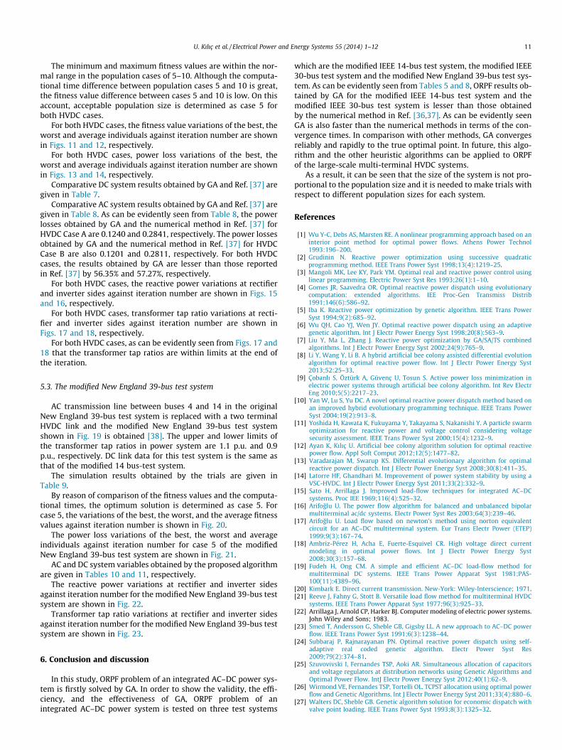
In this study, ORPF problem of an integrated AC–DC power sys-tem is firstly solved by GA. In order to show the validity, the effi-ciency, and the effectiveness of GA, ORPF problem of anintegrated AC–DC power system is tested on three test systems

which are the modified IEEE 14-bus test system, the modified IEEE30-bus test system and the modified New England 39-bus test sys-tem. As can be evidently seen from Tables 5 and 8, ORPF results ob-tained by GA for the modified IEEE 14-bus test system and themodified IEEE 30-bus test system is lesser than those obtainedby the numerical method in Ref. [36,37]. As can be evidently seenGA is also faster than the numerical methods in terms of the con-vergence times. In comparison with other methods, GA convergesreliably and rapidly to the true optimal point. In future, this algo-rithm and the other heuristic algorithms can be applied to ORPFof the large-scale multi-terminal HVDC systems.

As a result, it can be seen that the size of the system is not pro-portional to the population size and it is needed to make trials withrespect to different population sizes for each system.

References

[1] Wu Y-C, Debs AS, Marsten RE. A nonlinear programming approach based on aninterior point method for optimal power flows. Athens Power Technol1993:196–200.

[2] Grudinin N. Reactive power optimization using successive quadraticprogramming method. IEEE Trans Power Syst 1998;13(4):1219–25.

[3] Mangoli MK, Lee KY, Park YM. Optimal real and reactive power control usinglinear programming. Electric Power Syst Res 1993;26(1):1–10.

[4] Gomes JR, Saavedra OR. Optimal reactive power dispatch using evolutionarycomputation: extended algorithms. IEE Proc-Gen Transmiss Distrib1991;146(6):586–92.

[5] Iba K. Reactive power optimization by genetic algorithm. IEEE Trans PowerSyst 1994;9(2):685–92.

[6] Wu QH, Cao YJ, Wen JY. Optimal reactive power dispatch using an adaptivegenetic algorithm. Int J Electr Power Energy Syst 1998;20(8):563–9.

[7] Liu Y, Ma L, Zhang J. Reactive power optimization by GA/SA/TS combinedalgorithms. Int J Electr Power Energy Syst 2002;24(9):765–9.

[8] Li Y, Wang Y, Li B. A hybrid artificial bee colony assisted differential evolutionalgorithm for optimal reactive power flow. Int J Electr Power Energy Syst2013;52:25–33.

[9] Çobanlı S, Öztürk A, Güvenç U, Tosun S. Active power loss minimization inelectric power systems through artificial bee colony algorithm. Int Rev ElectrEng 2010;5(5):2217–23.

[10] Yan W, Lu S, Yu DC. A novel optimal reactive power dispatch method based onan improved hybrid evolutionary programming technique. IEEE Trans PowerSyst 2004;19(2):913–8.

[11] Yoshida H, Kawata K, Fukuyama Y, Takayama S, Nakanishi Y. A particle swarmoptimization for reactive power and voltage control considering voltagesecurity assessment. IEEE Trans Power Syst 2000;15(4):1232–9.

[12] Ayan K, Kılıç U. Artificial bee colony algorithm solution for optimal reactivepower flow. Appl Soft Comput 2012;12(5):1477–82.

[13] Varadarajan M, Swarup KS. Differential evolutionary algorithm for optimalreactive power dispatch. Int J Electr Power Energy Syst 2008;30(8):411–35.

[14] Latorre HF, Ghandhari M. Improvement of power system stability by using aVSC-HVDC. Int J Electr Power Energy Syst 2011;33(2):332–9.

[15] Sato H, Arrillaga J. Improved load-flow techniques for integrated AC–DCsystems. Proc IEE 1969;116(4):525–32.

[16] Arifoglu U. The power flow algorithm for balanced and unbalanced bipolarmultiterminal ac/dc systems. Electr Power Syst Res 2003;64(3):239–46.

[17] Arifoglu U. Load flow based on newton’s method using norton equivalentcircuit for an AC–DC multiterminal system. Eur Trans Electr Power (ETEP)1999;9(3):167–74.

[18] Ambriz-Pérez H, Acha E, Fuerte-Esquivel CR. High voltage direct currentmodeling in optimal power flows. Int J Electr Power Energy Syst2008;30(3):157–68.

[19] Fudeh H, Ong CM. A simple and efficient AC–DC load-flow method formultiterminal DC systems. IEEE Trans Power Apparat Syst 1981;PAS-100(11):4389–96.

[20] Kimbark E. Direct current transmission. New-York: Wiley-Interscience; 1971.[21] Reeve J, Fahny G, Stott B. Versatile load flow method for multiterminal HVDC

systems. IEEE Trans Power Apparat Syst 1977;96(3):925–33.[22] Arrillaga J, Arnold CP, Harker BJ. Computer modeling of electric power systems.

John Wiley and Sons; 1983.[23] Smed T, Andersson G, Sheble GB, Gigsby LL. A new approach to AC–DC power

flow. IEEE Trans Power Syst 1991;6(3):1238–44.[24] Subbaraj P, Rajnarayanan PN. Optimal reactive power dispatch using self-

adaptive real coded genetic algorithm. Electr Power Syst Res2009;79(2):374–81.

[25] Szuvovivski I, Fernandes TSP, Aoki AR. Simultaneous allocation of capacitorsand voltage regulators at distribution networks using Genetic Algorithms andOptimal Power Flow. IntJ Electr Power Energy Syst 2012;40(1):62–9.

[26] Wirmond VE, Fernandes TSP, Tortelli OL. TCPST allocation using optimal powerflow and Genetic Algorithms. Int J Electr Power Energy Syst 2011;33(4):880–6.

[27] Walters DC, Sheble GB. Genetic algorithm solution for economic dispatch withvalve point loading. IEEE Trans Power Syst 1993;8(3):1325–32.

12 U. Kılıç et al. / Electrical Power and Energy Systems 55 (2014) 1–12

[28] Goldberg DE. Genetic algorithms in search, optimization and machinelearning. Addison Wesley Publishing Company; 1989.

[29] Kumari MS, Maheswarapu S. Enhanced genetic algorithm based computationtechnique for multi-objective optimal power flow solution. Int J Electr PowerEnergy Syst 2010;32(6):736–42.

[30] Lu CN, Chen SS, Ong CM. The incorporation of HVDC equations in optimalpower flow methods using sequential quadratic programming techniques.IEEE Trans Power Syst 1988;3(3):1005–11.

[31] Mustafa MW, Abdul Kadir AF. A modified approach for load flow analysis ofintegrated AC–DC power systems. In: TENCON 2000. Proceedings, vol. 2; 2000.p. 108–13.

[32] Kundur P. Power system stability and control. New York: McGraw Hill; 1994.[33] Holland JH. Adaptation in natural and artificial systems. Ann Arbor: University

of Michigan Press; 1975.

[34] MATLAB Optimization Toolbox 5 User’s Guide. The Math Works, Inc.; 2012.[35] S�ahin AS�, Kılıç B, Kılıç U. Optimization of heat pump using fuzzy logic and

genetic algorithm. Heat Mass Transf 2011;47(12):1553–60.[36] Sreejaya P, Iyer SR. Optimal reactive power flow control for voltage profile

improvement in AC–DC power systems. In: Power Electronics, Drives andEnergy Systems (PEDES) 2010 Power India; 2010. p. 1–6.

[37] Taghavi R, Seifi A. Optimal reactive power control in hybrid power systems.Electr Power Compon Syst 2012;40(7):741–58.

[38] Lin YZ, Cai ZX, Mo Q. Transient stability analysis of ac/dc power system basedon transient energy function. In: Electric Utility Deregulation andRestructuring and Power Technologies (DRPT) 2008, Nanjuing; 2008. p.1103–8.