Contents lists available at ScienceDirect

Electrical Power and Energy Systems

journal homepage: www.elsevier.com/locate/ijepes

A practical method of transient stability analysis of stochastic power systemsbased on EEAC

Tong Huang⁎, Jie Wang⁎

School of Electronic Information and Electrical Engineering, Shanghai Jiao Tong University, Shanghai, China

A B S T R A C T

With the diversification of power systems and the application of power electronic technology, the uncertainty of power systems is becoming more and more serious,and the traditional deterministic transient stability analysis methods encounter severe challenges. In this paper, a practical method is proposed for transient stabilityanalysis of stochastic multi-machine systems based on EEAC. Firstly, the stochastic differential equation model of multi-machine systems is established. Secondly, thestochastic multi-machine system is equivalent to a stochastic single-machine infinite bus system according to coherency. Finally, the acceleration and decelerationarea is constructed, and Heun’s method is used to seek the critical clearing time of the system. The method is applied to analyse transient stability of four machinesystem. Compared with the numerical simulation based on Monte Carlo method, the simplicity and effectiveness of the method are verified. The impact of stochasticdisturbance intensity on stability is also presented.

1. Introduction

Power systems stability is influenced by the characteristics of eachmain component in the system [1–4]. Traditional power systems existstochastic disturbance such as load fluctuation, mechanical power sto-chastic torsional oscillation and measurement noise. With the con-tinuous expansion of the scale of the power grid, the access to renew-able energy, the application of power electronic devices and thepopularity of electric vehicles, the stochasticity of power systemscannot be ignored [5–7]. Therefore, the traditional deterministic tran-sient stability analysis method is facing severe challenges, and thepower system stochastic model and the stability analysis method con-sidering stochastic factors have attracted wide attention [7,8].

The stochasticity in the dynamic equations of power system ismainly expressed in 3 aspects [9,10]:

(a) The stochasticity of the initial value, caused by the uncertainty ofequilibrium points of power systems.

(b) The stochasticity of the parameters and coefficients of the stateequation is caused by the variation of the operating state and theinternal structure.

(c) Stochastic external excitation, such as conventional load fluctua-tion, renewable energy generation fluctuation, and charging loadfluctuation of electric vehicles.

The parameter and the initial value is constant for a dynamic pro-cess, and the solution of these two types is the Probabilistic differential

equation model, assuming the initial value and the parameters orcoefficients obey a certain probability distribution, the probability ofsystem stability or the envelope of the corresponding trajectory is ob-tained. And stochastic external excitation is characterized by rapidchange, and in the dynamic process it is considered to be a time vari-able. It needs to introduce stochastic differential equation theory formodelling and analysis [11]. In this paper, the impact of stochasticexternal excitation on power systems is studied.

Time-domain simulation and direct methods are used to analysepower system transient stability [12,13]. The direct methods mainlyincludes the EEAC methods and the energy function methods. EEAC as apractical transient stability criterion was first proposed in [14]. Thesedeterministic methods need to be modified in order to apply to theanalysis of power systems with stochastic disturbances. And EEAC isconstantly being improved and studied [15–17]. In the past decade,numerical integration methods have significant development to simu-late stochastic differential equations [18]. And a method using transientenergy function for stochastic power systems is proposed in [19]. Thefirst idea to use EEAC to analyse the probabilistic stability is proposedin [20], and a probability approach to discuss the probabilistic aspectsof transient stability evaluation of power systems combined EEAC andprobability density function (PDF) is proposed in [21], where the sto-chastic disturbance is a constant value instead of a time variable in thetransient process, and the stochastic differential equation theory is notintroduced into the power system research to frame stochastic form ofEEAC. An analysis of the evolution of the PDF of dynamic trajectories ofa single infinite bus power system is proposed in [22], where the time

https://doi.org/10.1016/j.ijepes.2018.11.011Received 8 May 2018; Received in revised form 5 September 2018; Accepted 8 November 2018

⁎ Corresponding authors.E-mail addresses: 251418920@qq.com (T. Huang), jiewangxh@sjtu.edu.cn (J. Wang).

Electrical Power and Energy Systems 107 (2019) 167–176

0142-0615/ © 2018 Elsevier Ltd. All rights reserved.

T

varying stability probability is decided by the PDF of state variables. Inthe transient analysis of actual systems. It is necessary to calculate thestability probability and the critical clearing time more quickly andaccurately. In this paper, the theory of EEAC and the stochastic dif-ferential equation theory will be merged and modified to present apractical approach to study the transient stability.

2. Stochastic power system model and numerical method

2.1. Ito stochastic differential equation model of power systems

In the dynamic process of power systems, the stochastic externalexcitation is mainly divided into the following categories:

(a) Mechanical power fluctuations;(b) Renewable energy output fluctuations;(c) Load fluctuations.

These fluctuations can cause fluctuations in the voltage, current andpower angle, and interfere with the stability of the power system.Suppose we write the disturbance vector as W t( ). The state variable ofthe power system is X , the state equation matrix with random excita-tion can be written as:

= +X A X ζ X Wt t t ( , ) ( , ) ( ) (1)

where A Xt( , ) is the deterministic state derivative function, and ζ Xt( , )is the disturbance function matrix, and ∈ WW t t( ) ( ) is generally as-sumed that it has the following properties:

(a) W t( ) is independent of each other at any two different time points;(b) W t{ ( )} is stable, and its joint distribution is independent of t ;(c) =E W t[ ( )] 0.

In order to meet the above requirements, W t( ) can be regarded as ageneralized stochastic process, that is, the white noise process. In thissection, suppose the stochastic disturbance source is the load fluctua-tion of the power system, and the load fluctuation is generally con-sidered to be a normal distribution [21]. Suppose W t σ t( )Ñ(0, )2 , when

=σ 1, that is ∼W t( ) t N(0, 1). So W t( ) is a standard Gauss whitenoise process. Discrete form of one dimensional diffusion of (1):

− = ++X X A t X t ζ t X W t( , )Δ ( , ) Δk k k k k k k k k1 (2)

where =X X t( )j j , =W W t( )k k , = −+t t tΔ k k k1 . Replace W tΔk k with= −+B B BΔ j j j1 , and it is easy to get that B t( ) has a stable independent

increment of mean zero. It is only Brownian motion that both meets theabove properties and has a continuous path. B t( ) follows the Brownianmovement, the project is also known as the Wiener process.

According to (2), the expression of state vector is:

∑ ∑= + +=

−

=

−

X X A t X t ζ t X B( , )Δ ( , )Δkj

k

j j jj

k

j j j00

1

0

1

(3)

when →tΔ 0j , the continuous form of (3) is:

∫ ∫= + +X X A s X ds ζ s X dB( , ) ( , )tt

st

s s0 0 0 (4)

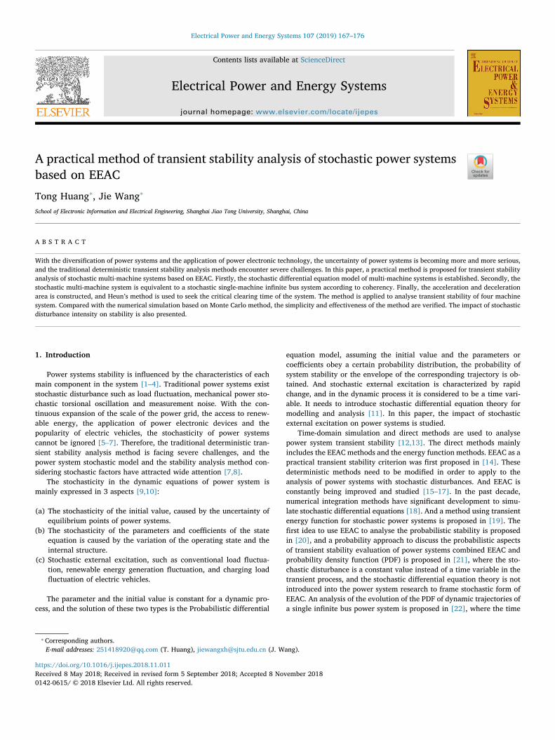
Which is also the integral form of the stochastic differential equa-tion of power systems. State vector can be regarded as a diffusionprocess in (4), where A is the drift coefficient, ζ is the diffusion coef-ficient. When step size =t msΔ 0.1 , The path of one dimensional stan-dard Gauss process and one dimensional standard Brownian motion isshown in Fig. 1.

Ito and Riemann have different rules of differentiation. Suppose X isan Ito process as follows:

= +dX udt vdB t( ) (5)

If ∈ ∞ ×g t x C R( , ) ([0, ) )2 , =Y g t X( , ) is a IT o process, which is

satisfied to:

=∂

∂+

∂

∂+

∂

∂dY

gt

t X dtgx

t X dXg

xt X dX( , ) ( , ) 1

2( , )·( )

2

22

(6)

where =dX dX dX( ) ( )·( )2 is computed according to the rules:

= = = =dt dt dt dB t dB t dt dB t dB t dt· · ( ) ( )· 0, ( )· ( ) (7)

2.2. Numerical methods of IT o stochastic differential equation

It o stochastic differential equations are the same as ordinary dif-ferential equations, only partial equations can be solved analytically,and the other part can only be solved by numerical methods. And thespecific results of the analytical solution of the stochastic differentialequation still need to be solved by numerical methods [23]. The maindifference of numerical methods of the stochastic differential equationcompared with the numerical methods of ordinary differential equa-tions is that the special properties of the Wiener process and the sto-chastic integral must be considered.

At present, the numerical integration method is commonly used:Euler-Maruyama (EM) method, Milstein method, Huen’s method, andRunge-Kutta method [18]. EM method is the simplest numericalmethod, but it has lower convergence order. Huen’s method is based onthe trapezoidal formula, which improves the convergence order by firstpredicting the post correction. For the diffusion process of (1), thenumerical iterative scheme of the Huen’s method is:

(a) First prediction:

= ++X X A X ζ X Bt + ( )Δ ( )Δi i i i i1 (8)

(b) Correction to get the iteration value:

=+

++

++ +X X A X A X ζ X ζ X

Bt+ ( ) ( )

2Δ

( ) ( )2

Δi ii i i i

i11 1

(9)

where =A X A Xt ,( ) ( )i i , =ζ X ζ Xt ,( ) ( )i i , +A X( )i 1 and +ζ X( )i 1 is pre-dictive value, Taking white Guassian noise as an example, BΔ i is theBrownian movement increment, that is ∼B NΔ Δt (0, 1)i . Huen’smethod is also applicable to the simulation under other white non-Gauss noise (such as Poisson white noise), but it needs to pay attentionto the difference among different types of white noise in the MonteCarlo simulation.

3. The equivalence method of stochastic power systems

3.1. Stochastic model of multi machine system

Rotor equation is an effective tool of power system transient stabi-lity research. In this paper, the transient stability is considered only ifthe first swing is unstable, where the effect of the damping is neglected.Suppose that the transient potential ′E i remains constant during thetransient process. In the case of stochastic disturbance, the rotor motionequation of the first i generator is:

= −M d δdt

P Pii

M i e i2

2 , , (10)

The electromagnetic power of the first i generator is:

∑= ′ + ′ ′ − −= ≠

P E G E E Y δ δ αsin( )e i i ii ii j i

n

j ij i j ij,2

1, (11)

The performance of external stochastic excitations is a stochasticpower disturbance on the rotor motion equation. The rotor equations ofthe first i generator with stochastic disturbance are considered:

= − +M d δdt

P P PiM i e i c i

2

2 , , , (12)

T. Huang, J. Wang Electrical Power and Energy Systems 107 (2019) 167–176

168

where Pc i, is stochastic power fluctuation of the first i generating setcaused by the external stochastic excitations. Load fluctuation is chosenas the source of stochastic disturbance, and the load fluctuation isgenerally regarded as a Gauss process [24]. Let =P ζ W t( )c i i, . Accordingto the operation data of power system, selecting the appropriate sampleand the sufficient sample quantity, the complete probability space canbe established by analysing the law of stochastic power fluctuation, andthe stochastic disturbance intensity ζi can be obtained by the similarityprinciple [25]. The rotor equations can be written as:

= − +M d δdt

P P ζ W t( )iM i e i i

2

2 , , (13)

In this paper, we consider only the impact of white Guassian noisewhich is normal distribution, but other distributions can be in-corporated. For instance, wind generation is often suggested to be aWeibull distribution [26], whereas Plug-in electric vehicles have beensupposed to be Poisson distribution [5].

For the stochastic disturbance of white Poisson noise type, the ex-pression is:

∑= −=

C t R δ t T( ) ( )i

N t

i i1

( )

(14)

where N t( ) is the Poisson counting process, the number of pulses ar-riving in [0, t], and the average arrival rate >λ 0, ⩾R i{ , 1}i are ex-pressed as the pulse amplitude that obeys a certain probability dis-tribution. The numerical simulation method is shown in the literature[24], and Ri is taken as the normal distribution. The rotor motionequation is changed into:

= − +M d δdt

P P ζ C t( )iM i e i i

2

2 , , (15)

3.2. Equivalent method of stochastic multi machine systems

Because of the direct application of Monte Carlo method have somelimitations on dimension and computation time, it is very important tostudy the new method to analyse transient stability. Inspired by thepractical stability criterion EEAC of the deterministic system, the sto-chastic multi-machine system is simplified and the equivalence is car-ried out. When a fault occurs or a fault is clear, according to Coherenceand the results of large step integration the generators can be dividedinto group S and group a. Assume that damping is ignored, theequivalent value can be obtained by the following method:

Assuming that the stochastic disturbances are independent of eachother, the equations of motion of each generator set in group S can be

added together:

∑ ∑ ∑= − +∈ ∈ ∈

ddt

M δ P P ζ W t( ) ( )i S

i ii S

M i e ii S

i

2

2 , ,(16)

Because the linear combination of multiple independent Gaussprocesses is still a Gauss process, so let = ∑ ∈

ζ W t ζ W t( ) ( )S i S i , (16)could be transformed to:

= − +M d δdt

P P ζ W t( )SS

M S e S S

2

2 , , (17)

where

∑ ∑ ∑= =∑

∑= =

∈

∈

∈ ∈ ∈

M M δM δM

P P P P, , ,Si s

i Si s i i

i s iM S

i SM i e S

i Se i, , , ,

In the same way, the equivalent rotor motion equation of group a:

= − +M d δdt

P P ζ W t( )aa

M a e a a

2

2 , , (18)

(17) and (18) can be regarded as a two machine system, ζ W t( )S andζ W t( )a are equivalent stochastic disturbance of equivalent units of

corresponding groups. Let = −δ δ δs a, that is = −d δdt

d δdt

d δdt

S a22

22

22 . (17)

minus (18), we have

= − ′ +M d δdt

P P ζW t( )M e2

2 (19)

where

=+

M M MM M

S a

S a

=+

−+

P MM M

P MM M

PMa

S aM S

S

S aM a, ,

′ =+

−+

P MM M

P MM M

Pea

S ae S

S

S ae a, ,

And the equivalence of random disturbance intensity:

∑ ∑=+

−+

∈ ∈

ζW t MM M

ζ W t MM M

ζ W t( ) ( ) ( )a

S a i Si

S

S a j aj

(20)

At this point, based on the EEAC equivalence principle, theequivalent method of stochastic disturbance is derived. ζW t( ) isequivalent stochastic disturbance of the equivalent single-machine in-finite system (SMIB) system, ζ is equivalent stochastic disturbance in-tensity, it follows the algorithm of stochastic variables. Because of

′ = + −P P P δ υsin( )e me max , which contains the invariant part, it is se-parated into the equivalent mechanical power, we can get the equation:

0 2 4-0.05

0

0.05

t

W(t)

0 1 2 3 4 5-1

0

1

2

3

4

5

t

B(t)

Fig. 1. Standard Gauss white noise and Corresponding path of Brownian motion.

T. Huang, J. Wang Electrical Power and Energy Systems 107 (2019) 167–176

169

= − +M d δdt

P P ζW t( )m e2

2 (21)

The specific process of equivalence is shown in EEAC part of theappendix. The equivalent method is still applicable to the other additivewhite noise, such as Poisson white noise, and it is worth noting thatdifferent types of white noise are different when calculating (20).

4. Modified EEAC

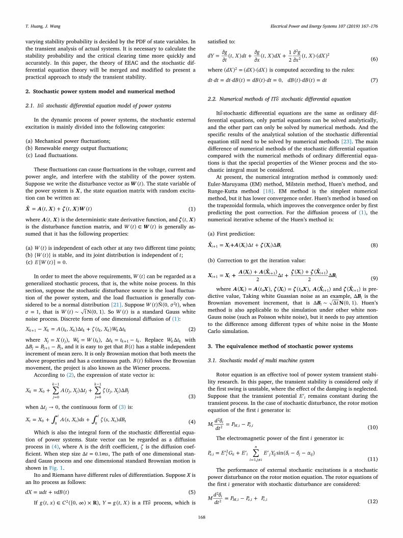
Stochastic complex systems can be equivalent to a stochastic SMIBsystem by the method of the previous section, and the transient stabilityof the equivalent SMIB system can be studied by Equal-Area Criteria[27]. Due to the time-varying stochastic disturbance, the UEP of thesystem cannot be directly determined, that is, the maximum decelera-tion area can not be calculated by the deterministic method. The re-search object in this section is a SMIB system. The structure is shown inFig. 2. The detailed parameters are shown in the article [28]. Loadfluctuation is also a stochastic disturbance source, damping neglected,considering whether the first swing is unstable.

Considering one dimensional stochastic disturbance, the two ordermodel of the generator in the transient process:

= − +M d δdt

P P ζW t( )m ei2

2 (22)

where =i 1, 2, 3 respectively indicate pre-fault, during the fault andafter fault clearance. Assuming that the system is in steady state at pre-fault, the accelerating area under stochastic disturbance can be calcu-lated by stochastic differential formula. According to (5)–(7), the ac-celerating area can be written:

∫ ∫= +S M ωdω dω( 12

( ) )a ω

ω

ω

ω 2c c

0 0 (23)

The acceleration area can also be written as follows:

∫ ∫ ∫= − + +S P P δ ωdt ζ ωdB tM

ζ dt( sin ) ( ) 12a t

tm e t

t

t

t2

2c c c

0 0 0 (24)

Similarly, deceleration area can be written as the following form:

∫ ∫ ∫= − − −S P δ P ωdt ζ ωdB tM

ζ dt( sin ) ( ) 12d t

te m t

t

t

t3

2c

u

c

u

c

u

(25)

As mentioned above, a formula for calculating the acceleration anddeceleration area with Ito integral is proposed. When tu corresponds tothe return point, Sd is the deceleration area. When tu corresponds to thenearest unstable equilibrium point, Sd is the maximum decelerationarea. When the system is stable or critical stable, the acceleration areaof the system is equal to the deceleration area and smaller than themaximum deceleration area. The latter two terms of (24) and (25) re-flect the difference between Ito integral and Riemann integral. Sto-chastic disturbance caused unpredictable area fluctuation, so the ana-lytical method cannot solve the acceleration and deceleration area. Theabove deduction is aimed at the stochastic disturbance of Gauss whitenoise type. If the stochastic disturbance is Poisson white noise or othertypes of white noise, we need to derive the corresponding stochasticdifferential rule. Huen’s method has good numerical stability and strongconvergence for solving stochastic differential equations, so it can besolved by the Huen’s method to solve the acceleration and decelerationarea.

This paper presents a modified EEAC method for the transient sta-bility analysis of stochastic multi machine systems:

1) According to the complex system operation parameters and faultconditions, all generators are divided into two coherent groups indifferent periods, and take simplification and equivalence on sys-tems respectively, Then parameters of the equivalent SMIB systemare obtained, so acceleration area Sa and deceleration area Sd areable to be calculated;

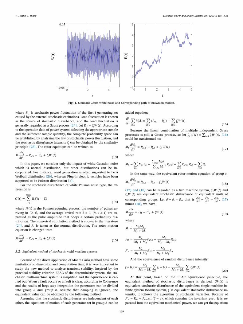
2) If the range of CCTs is known, as shown in Fig. 3, ∈t [0.06, 0.12]cr ,and the step size is dt . From the time of resection, use (18)–(19) andHuen’s method to obtain the corresponding trajectory of the accel-eration and deceleration area;

3) If areas are equal, set the clearing time for +t dtcrb . Loop until thefirst time when − >S S 0a d (i.e., the corresponding separation pointof the acceleration and deceleration area in Fig. 3). And the corre-sponding clearing time is the CCT on this stochastic process.

The accuracy of CCTs is decided by the step size of the clearing time.When the stochastic disturbance intensity is 0.001, the accelerationarea and deceleration area changes as shown in Fig. 3. The corre-sponding clearing time is the CCT on this stochastic process.

As shown in Fig. 4, due to the existence of stochastic disturbance,the acceleration area and deceleration area have a fluctuation, the se-paration points under 10 runs have also been a big wave. This showsthat the CCTs of power systems is not a fixed value in the case of sto-chastic disturbance.

5. Case study

The system of four machines two areas is used for case study, asshown in Fig. 5, and specific parameters are shown in appendix [28].Fault is set in one line of double line on bus 6 to bus 7 which is near tobus 7, the fault type is three-phase short circuit.

Under this fault, group S contains no. 1, 2 machines, other machinesare in group a. Fault clearing time is set to be 0.195 s, and the relativeangle curve of G1 and G3 without stochastic disturbance is calculated,as thick lines shown in Fig. 6, indicating that the system is stable. In thecase of stochastic disturbance, the angle curves after the 100 runs areshown in Fig. 6. It can be seen that under some stochastic processes, thesystem is stable, but in other cases it is unstable. This phenomenonindicates that the stability of the system is no longer a single stable andunstable state in the case of stochastic disturbance, and it needs to bedescribed by the stability probability. Under different stochastic paths,

generator transformer

infinite system

busline

Fig. 2. The diagram of a SMIB system.

Fig. 3. The curves of Acceleration and deceleration area when ζ is 0.001 (1run).

T. Huang, J. Wang Electrical Power and Energy Systems 107 (2019) 167–176

170

the critical clearing time is also different. After 1000 runs, the CCTs arecounted, and the frequency distribution diagram is shown in Fig. 7.Therefore, the stochastic disturbance has an impact on transient stabi-lity. The impact need to be quantified.

In order to verify the effectiveness of the method proposed in thispaper, the numerical simulation based on Monte Carlo method iscompared with modified EEAC. The results obtained by using the MCmethod are shown in Fig. 8. The results of the two methods are shownin Table 1. It can be seen that the mean value, standard deviation,maximum value and minimum value of the statistics are consistentwithin the error range, which verifies the correctness and effectivenessof the proposed method.

Two methods are conducted in .m file of Matlab R2012a, where theCPU is Intel Core i5, the memory is 8 G, and the operating system isWindows 10. The contrast of cputime shows the advantage of theproposed method in terms of algorithm efficiency. And this advantagewill become more evident when the system continues to expand.

The stochastic disturbance intensity are set to different times of theinitial value to study its impact on stability using modified EEAC. By1000 runs, the maximum and minimum variation is shown in Fig. 9under different stochastic disturbance intensity. It can be seen that,with the increase of the intensity, the uncertainty of CCTs is also in-creased. The statistics of CCTs are shown in Table 2. As shown inFig. 10, the standard deviation becomes larger with the increase of the

stochastic disturbance intensity. And according to the phenomenon ofthis approximate linear growth trend, the standard deviation CCTscould be estimated under a certain stochastic disturbance intensity.

According to the law of large number of Bernoulli, the probabilitydensity distribution can be approximated by the frequency distribution.

Fig. 4. The results of tcr (10 runs).

~ ~

~ ~

G1

4G2G

G31

2

3

4

65 7 8 9 10 1125km 20km 110km 110km 20km 25km

L7 C7 C9 L9

Fig. 5. The diagram of the case system.

1 1.5 2 2.5 3 3.5 4 4.5 5

-150

-100

-50

0

50

100

150

Time(s)

Rot

or a

ngle

(deg

ree)

G1

G3

Fig. 6. The relative rotor angle curves of G1 and G3 with and without stochasticdisturbance (100 runs).

Fig. 7. Frequency distribution histogram of tcr based on results of modifiedEEAC.

T. Huang, J. Wang Electrical Power and Energy Systems 107 (2019) 167–176

171

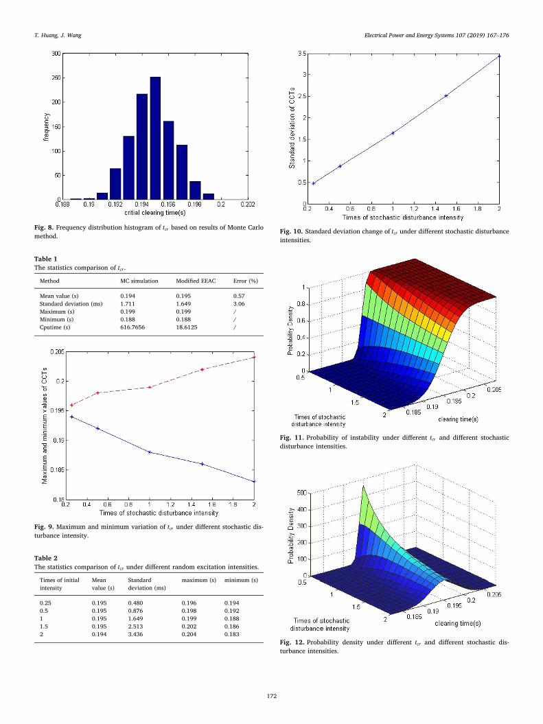
Fig. 8. Frequency distribution histogram of tcr based on results of Monte Carlomethod.

Table 1The statistics comparison of tcr .

Method MC simulation Modified EEAC Error (%)

Mean value (s) 0.194 0.195 0.57Standard deviation (ms) 1.711 1.649 3.06Maximum (s) 0.199 0.199 /Minimum (s) 0.188 0.188 /Cputime (s) 616.7656 18.6125 /

Fig. 9. Maximum and minimum variation of tcr under different stochastic dis-turbance intensity.

Table 2The statistics comparison of tcr under different random excitation intensities.

Times of initialintensity

Meanvalue (s)

Standarddeviation (ms)

maximum (s) minimum (s)

0.25 0.195 0.480 0.196 0.1940.5 0.195 0.876 0.198 0.1921 0.195 1.649 0.199 0.1881.5 0.195 2.513 0.202 0.1862 0.194 3.436 0.204 0.183

Fig. 10. Standard deviation change of tcr under different stochastic disturbanceintensities.

Fig. 11. Probability of instability under different tcr and different stochasticdisturbance intensities.

Fig. 12. Probability density under different tcr and different stochastic dis-turbance intensities.

T. Huang, J. Wang Electrical Power and Energy Systems 107 (2019) 167–176

172

Applied probability fitting, the relationship between different stochasticdisturbance and stability probability is obtained. As shown inFigs. 11,12, the earlier the fault is removed, the greater the probabilityof stability. According to the results of the deterministic method,

=t s0. 195cr , and taking into account the error of action, generally setaction time of circuit breakers to be 0.190 s in the project. Under the0.5, 1 times of the initial intensity, the probability of transient in-stability is about 0%, but the probability is 1.23% under 1.5 times of theinitial intensity, and the probability of instability is 4.97% under 2times of the initial intensity. The greater the stochastic disturbanceintensity, the larger the standard deviation. In order to meet the re-quirements of stability, the action time should be in advance.

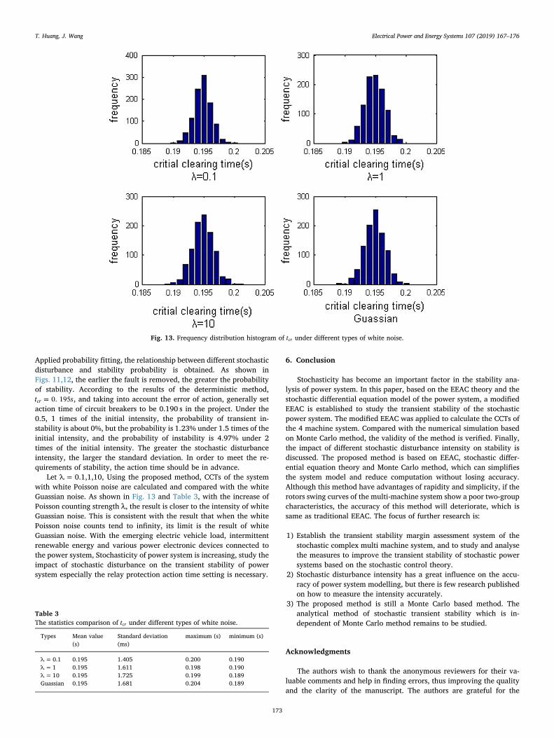
Let λ=0.1,1,10, Using the proposed method, CCTs of the systemwith white Poisson noise are calculated and compared with the whiteGuassian noise. As shown in Fig. 13 and Table 3, with the increase ofPoisson counting strength λ, the result is closer to the intensity of whiteGuassian noise. This is consistent with the result that when the whitePoisson noise counts tend to infinity, its limit is the result of whiteGuassian noise. With the emerging electric vehicle load, intermittentrenewable energy and various power electronic devices connected tothe power system, Stochasticity of power system is increasing, study theimpact of stochastic disturbance on the transient stability of powersystem especially the relay protection action time setting is necessary.

6. Conclusion

Stochasticity has become an important factor in the stability ana-lysis of power system. In this paper, based on the EEAC theory and thestochastic differential equation model of the power system, a modifiedEEAC is established to study the transient stability of the stochasticpower system. The modified EEAC was applied to calculate the CCTs ofthe 4 machine system. Compared with the numerical simulation basedon Monte Carlo method, the validity of the method is verified. Finally,the impact of different stochastic disturbance intensity on stability isdiscussed. The proposed method is based on EEAC, stochastic differ-ential equation theory and Monte Carlo method, which can simplifiesthe system model and reduce computation without losing accuracy.Although this method have advantages of rapidity and simplicity, if therotors swing curves of the multi-machine system show a poor two-groupcharacteristics, the accuracy of this method will deteriorate, which issame as traditional EEAC. The focus of further research is:

1) Establish the transient stability margin assessment system of thestochastic complex multi machine system, and to study and analysethe measures to improve the transient stability of stochastic powersystems based on the stochastic control theory.

2) Stochastic disturbance intensity has a great influence on the accu-racy of power system modelling, but there is few research publishedon how to measure the intensity accurately.

3) The proposed method is still a Monte Carlo based method. Theanalytical method of stochastic transient stability which is in-dependent of Monte Carlo method remains to be studied.

Acknowledgments

The authors wish to thank the anonymous reviewers for their va-luable comments and help in finding errors, thus improving the qualityand the clarity of the manuscript. The authors are grateful for the

Fig. 13. Frequency distribution histogram of tcr under different types of white noise.

Table 3The statistics comparison of tcr under different types of white noise.

Types Mean value(s)

Standard deviation(ms)

maximum (s) minimum (s)

λ=0.1 0.195 1.405 0.200 0.190λ=1 0.195 1.611 0.198 0.190λ=10 0.195 1.725 0.199 0.189Guassian 0.195 1.681 0.204 0.189

T. Huang, J. Wang Electrical Power and Energy Systems 107 (2019) 167–176

173

financial support provided by the National Natural Science Foundationof China under grant 61374155 and the Specialized Research Fund for

the Doctoral Program of Higher Education of China under grant20130073110030.

Appendix

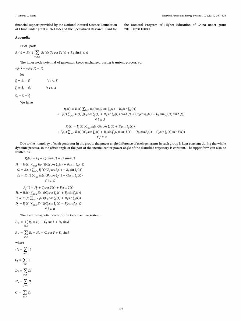
EEAC part:

∑= +∈

P t E t E t G δ t B δ t( ) ( ) ( )( cos ( ) sin ( ))ei ik S a

k ik ik ik ik,

The inner node potential of generator keeps unchanged during transient process, so:

= =E t E E t E( ) ( )i i k k

let

= − ∀ ∈ξ δ δ i Si i s

= − ∀ ∈ξ δ δ j aj j a

= −ξ ξ ξij i j

We have

= ∑ +

+ ∑ + + −

∀ ∈

∈

∈

P t E t E t G ξ t B ξ tE t E t G ξ t B ξ t δ t B ξ t G ξ t δ t

i S

( ) ( ) ( )( cos ( ) sin ( ))( ) ( )(( cos ( ) sin ( )) cos ( ) ( cos ( ) sin ( )) sin ( ))

ei i k S k ik ik ik ik

i j a j ij ij ij ij ij ij ij ij

= ∑ +

+ ∑ + − −

∀ ∈

∈

∈

P t E t E t G ξ t B ξ t

E t E t G ξ t B ξ t δ t B ξ t G ξ t δ tj a

( ) ( ) ( )( cos ( ) sin ( ))

( ) ( )(( cos ( ) sin ( )) cos ( ) ( cos ( ) sin ( )) sin ( ))ej j l a l jl jl jl jl

j i S i ji ji ji ji ji ji ji ji

Due to the homology of each generator in the group, the power angle difference of each generator in each group is kept constant during the wholedynamic process, so the offset angle of the part of the inertial center power angle of the disturbed trajectory is constant. The upper form can also bewritten as:

= + +

= ∑ +

= ∑ +

= ∑ −

∀ ∈

∈

∈

∈

P t H C δ t D δ t

H E t E t G ξ t B ξ tC E t E t G ξ t B ξ t

D E t E t B ξ t G ξ t

i S

( ) cos ( ) sin ( )

( ) ( )( cos ( ) sin ( ))( ) ( )( cos ( ) sin ( ))

( ) ( )( cos ( ) sin ( ))

ei i i i

i i k S k ik ik ik ik

i i j a j ij ij ij ij

i i j a j ij ij ij ij

= + +

= ∑ +

= ∑ +

= ∑ −

∀ ∈

∈

∈

∈

P t H C δ t D δ tH E t E t G ξ t B ξ t

C E t E t G ξ t B ξ t

D E t E t G ξ t B ξ tj a

( ) cos ( ) sin ( )( ) ( )( cos ( ) sin ( ))

( ) ( )( cos ( ) sin ( ))

( ) ( )( sin ( ) cos ( ))

ej j j j

j j l a l jl jl jl jl

j j i S i ji ji ji ji

j j i S i ji ji ji ji

The electromagnetic power of the two machine system:

∑= = + +∈

P P H C δ D δcos sine Si S

ei S S S,

∑= = + +∈

P P H C δ D δcos sine aj a

ej a a a,

where

∑=∈

H HSi S

i

∑=∈

C CSi S

i

∑=∈

D DSi S

i

∑=∈

H Haj a

j

∑=∈

C Caj a

j

T. Huang, J. Wang Electrical Power and Energy Systems 107 (2019) 167–176

174

∑=∈

D Daj a

j

Then the two machine system is transformed into SMIB system by using the formula. The electromagnetic power of the equivalent SMIB systemcan be expressed as

′ = + −P P P δ υsin( )e c max

where

=−

+P M H M H

M Mca S S a

S a

= +P C Dmax2 2

= −−υ CD

tan ( )1

=−

+C M C M C

M Ma S S a

S a

=−

+D M D M D

M Ma S S a

S a

The mechanical power of the equivalent SMIB system can be expressed as

=−

+P

M P M PM MM

a M S S M a

S a

, ,

Under the assumption of classical model and two-group model, PM , Pc, Pmax, υ is constant, so we have

= − − − +M d δdt

P P P δ υ ζW tsin( ) ( )M c2

2 max

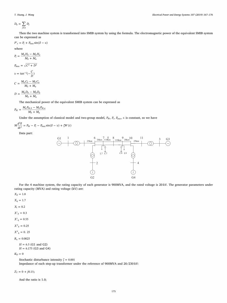
Data part:

~ ~

~ ~G1

G2 G4

G31

2

3

4

6 57 8 9 10 1125km 20km 110km 110km 20km 25km

L7 C7 C9 L9

For the 4 machine system, the rating capacity of each generator is 900MVA, and the rated voltage is 20 kV. The generator parameters underrating capacity (MVA) and rating voltage (kV) are:

=X 1.8d

=X 1.7q

=X 0.2l

′ =X 0.3d

′ =X 0.55q

″ =X 0.25d

″ =X 0. 25q

=R 0.0025a

=H 6.5 (G1 and G2)=H 6.175 (G3 and G4)

=K 0D

Stochastic disturbance intensity =ζ 0.001Impedance of each step-up transformer under the reference of 900MVA and 20/230 kV:

= +Z j0 0.15T ;

And the ratio is 1.0;

T. Huang, J. Wang Electrical Power and Energy Systems 107 (2019) 167–176

175

The length of the line has been marked, and the p.u. value of the line parameters under the reference of 900MVA and 230 kV is:

=r 0.0001 pu/km

=x 0.001 pu/kmL

=b /2 0.00175 pu/kmc

Electric potential of the inner node of a generator and active power under rating capacity (MVA) and rating voltage (kV):G1: ′ = +E j0.9466 0.5891q =P 0.7873G2: ′ = +E j1.0293 0.4251q =P 0.7847G3: ′ = +E j1.1087 0.1016q =P 0.8034G4: ′ =E j1.0988 - 0.0950q =P 0.7718Parameter of constant impedance model equalled to the load and reactive power of shunt capacitors of node 7 and 9:

= +y j1.0744 0.11117

= +y j1.9633 0.27789

References

[1] Billinton R, Kuruganty PRS. Probabilistic assessment of transient stability in apractical multimachine system. IEEE Trans Power Apparatus Syst 2010;1(7). 61 61.

[2] Wu F, Tsai YK. Probabilistic dynamic security assessment of power systems-I: basicmodel. IEEE Trans Circuits Syst 1983;30(3):148–59.

[3] Timko KJ, Bose A, Anderson PM. Monte Carlo Simulation of power system stability.IEEE Trans Power Apparatus Syst 1983;102(10):3453–9.

[4] Meldorf M, Taht T, Kilter J. Stochasticity of the electrical network load. Oil Shale2007;24(2s):225–36.

[5] Vlachogiannis JG. Probabilistic constrained load flow considering integration ofwind power generation and electric vehicles. IEEE Trans Power Syst2009;24(4):1808–17.

[6] Mohammed H, Nwankpa CO. Stochastic analysis and simulation of grid-connectedwind energy conversion system. IEEE Trans Energy Convers 2000;15(1):85–90.

[7] Faried SO, Billinton R, Aboreshaid S. Probabilistic evaluation of transient stability ofa wind farm. IEEE Trans Energy Convers 2009;24(3):733–9.

[8] Hockenberry JR, Lesieutre BC. Evaluation of uncertainty in dynamic simulations ofpower system models: the probabilistic collocation method. IEEE Trans Power Syst2004;19(3):1483–91.

[9] Zhang JY, Ju P, Yu YP, et al. Responses and stability of power system under smallGauss type random excitation. Sci China Technol Sci 2012;55(7):1873–80.

[10] Ming Z, Bo Y, Zhang X, et al. Stochastic small signal stability analysis of wind powerintegrated power systems based on stochastic differential equations. Procee CSEE2014;34(10):1575–82.

[11] Liu Y, Ping JU, Xue Y, et al. Calculation analysis on power system characteristicsunder random excitation. Automat Electric Power Syst 2014;38(9):137–42.

[12] Ribbens-Pavella M, Murthy PGK. Transient stability of power systems: theory andpractice. New York, NY (United States): John Wiley and Sons; 1994. 33(97):294 -299.

[13] Khedkar MK, Dhole GM, Neve VG. Transient stability analysis by transient energyfunction method: closest and controlling unstable equilibrium point approach. J

Instit Eng Electr Eng Division 2004;85(2):83–8.[14] Xue Y, Van Custem T, Ribbens-Pavella M. Extended equal area criterion justifica-

tions, generalizations, applications. IEEE Trans Power Syst 1989;4(1):44–52.[15] Xue Y, Wehenkel L, Belhomme R, et al. Extended equal area criterion revisited

[EHV power systems]. IEEE Trans Power Syst 1992;7(3):1012–22.[16] Xu Y, Dong ZY, Zhang R, et al. A decomposition-based practical approach to

transient stability-constrained unit commitment. IEEE Trans Power Syst2015;30(3):1455–64.

[17] Yin M, Chung CY, Wong KP, et al. An improved iterative method for assessment ofmulti-swing transient stability limit. IEEE Trans Power Syst 2011;26(4):2023–30.

[18] Higham DJ. An algorithmic introduction to numerical simulation of stochasticdifferential equations. Soc Indust Appl Math 2001;43:525–46.

[19] Odun-Ayo T, Crow ML. Structure-preserved power system transient stability usingstochastic energy functions. IEEE Trans Power Syst 2012;27(3):1450–8.

[20] Billinton R, Kuruganty PRS. Probabilistic evaluation of transient stability in amultimachine power system. Proc Inst Electr Eng 1979;126(4):321–6.

[21] Chiodo E, Lauria D. Transient stability evaluation of multimachine power systems: aprobabilistic approach based upon the extended equal area criterion. IEE Procee –Generation, Trans Distribut 1994;141(6):545–53.

[22] Wang K, Crow ML. The Fokker-Planck equation for power system stability prob-ability density function evolution. IEEE Trans Power Syst 2013;28(3):2994–3001.

[23] Milano F, Zarate-Minano R. A systematic method to model power systems as sto-chastic differential algebraic equations. IEEE Trans Power Syst2013;28(4):4537–44.

[24] Dong ZY, Zhao JH, Hill DJ. Numerical simulation for stochastic transient stabilityassessment. IEEE Trans Power Syst 2012;27(4):1741–9.

[25] Peng Yunjian, Zeng Jun, Deng Feiqi. A numeric method for stochastic transientstability analysis of excitation control system. Procee CSEE 2011;31(19):60–6.

[26] Burton T, Sharpe D, Jenkins N, et al. Wind energy handbook. Wiley; 2001.[27] Willems JL. Generalisation of the equal-area criterion for synchronous machines.

Proc Inst Electr Eng 1969;116(8):1431–2.[28] Kundur P. Power system stability and control. New York: McGraw-Hill lnc; 1994.

T. Huang, J. Wang Electrical Power and Energy Systems 107 (2019) 167–176

176