Electric Potential

(Chapter 25)

• Electric potential energy, U

• Electric potential energy in a constant field

• Conservation of energy

• Electric potential, V

• Relation to the electric field strength

• The potential of a point charge

• Calculating the potential of

• Multiple point charges

• Continuous distributions of charge

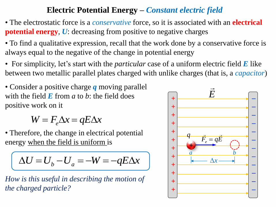
Electric Potential Energy – Constant electric field

• The electrostatic force is a conservative force, so it is associated with an electrical

potential energy, U: decreasing from positive to negative charges

• To find a qualitative expression, recall that the work done by a conservative force is

always equal to the negative of the change in potential energy

• For simplicity, let’s start with the particular case of a uniform electric field E like

between two metallic parallel plates charged with unlike charges (that is, a capacitor)

• Consider a positive charge q moving parallel

with the field E from a to b: the field does

positive work on it

• Therefore, the change in electrical potential

energy when the field is uniform is

How is this useful in describing the motion of

the charged particle?

b aU U U W qE x

eW F x qE x

+

+

+

+

+

+

+

+

+

+

+

+

–

–

–

–

–

–

–

–

–

–

–

–

E

eF qE+

Δx

q

a b

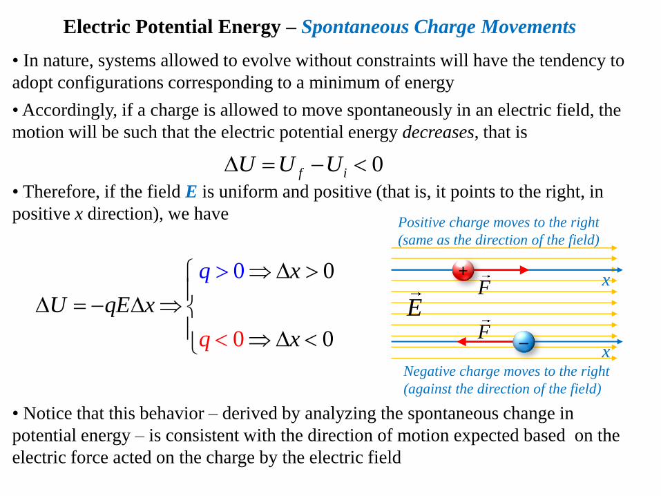
Electric Potential Energy – Spontaneous Charge Movements

• In nature, systems allowed to evolve without constraints will have the tendency to

adopt configurations corresponding to a minimum of energy

• Accordingly, if a charge is allowed to move spontaneously in an electric field, the

motion will be such that the electric potential energy decreases, that is

• Therefore, if the field E is uniform and positive (that is, it points to the right, in

positive x direction), we have

E

0

0 0

0 x

U qE x

q

q x

x

Positive charge moves to the right

(same as the direction of the field)

• Notice that this behavior – derived by analyzing the spontaneous change in

potential energy – is consistent with the direction of motion expected based on the

electric force acted on the charge by the electric field

0f iU U U

F

Negative charge moves to the right

(against the direction of the field)

Fx

+

–

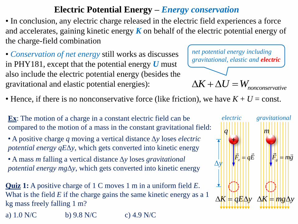
Electric Potential Energy – Energy conservation

• In conclusion, any electric charge released in the electric field experiences a force

and accelerates, gaining kinetic energy K on behalf of the electric potential energy of

the charge-field combination

Ex: The motion of a charge in a constant electric field can be

compared to the motion of a mass in the constant gravitational field:

• A positive charge q moving a vertical distance Δy loses electric

potential energy qEΔy, which gets converted into kinetic energy

• A mass m falling a vertical distance Δy loses gravitational

potential energy mgΔy, which gets converted into kinetic energy

K qE y

nonconservativeK U W

net potential energy including

gravitational, elastic and electric

Quiz 1: A positive charge of 1 C moves 1 m in a uniform field E.

What is the field E if the charge gains the same kinetic energy as a 1

kg mass freely falling 1 m?

a) 1.0 N/C b) 9.8 N/C c) 4.9 N/C

+

eF qE

electric gravitational

q m

gF mg

K mg y

Δy

• Hence, if there is no nonconservative force (like friction), we have K + U = const.

• Conservation of net energy still works as discusses

in PHY181, except that the potential energy U must

also include the electric potential energy (besides the

gravitational and elastic potential energies):

+ + + + + + + + + + + + + + +

– – – – – – – – – – – – – – – –

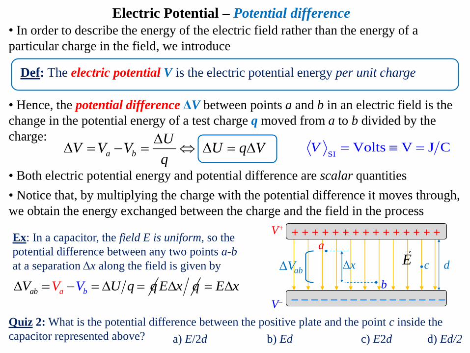
Electric Potential – Potential difference

• Hence, the potential difference ΔV between points a and b in an electric field is the

change in the potential energy of a test charge q moved from a to b divided by the

charge:

• Both electric potential energy and potential difference are scalar quantities

• Notice that, by multiplying the charge with the potential difference it moves through,

we obtain the energy exchanged between the charge and the field in the process

a b

UV V V U q V

q

SIVolts V J CV

Def: The electric potential V is the electric potential energy per unit charge

• In order to describe the energy of the electric field rather than the energy of a

particular charge in the field, we introduce

Ex: In a capacitor, the field E is uniform, so the

potential difference between any two points a-b

at a separation Δx along the field is given by

a bab V U q qVV E x q E x

d

Quiz 2: What is the potential difference between the positive plate and the point c inside the

capacitor represented above?

V+

V–

a

b

Δx EΔVab

a) E/2d b) Ed c) E2d d) Ed/2

c

+ + + + + + + + + + + + + + +

– – – – – – – – – – – – – – – –

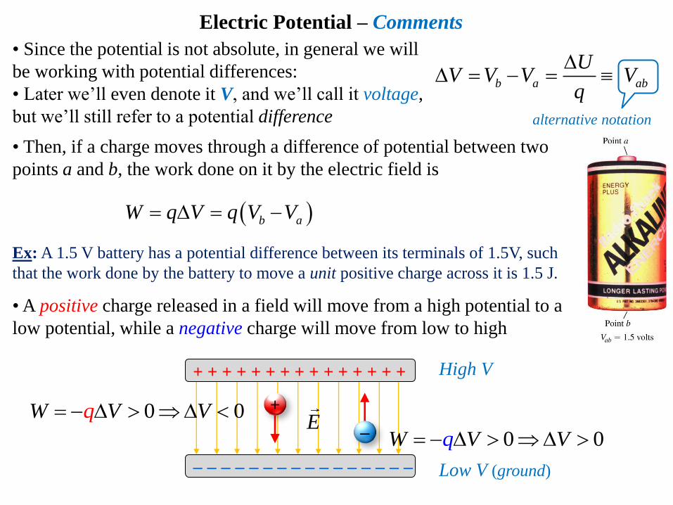
• Since the potential is not absolute, in general we will

be working with potential differences:

• Later we’ll even denote it V, and we’ll call it voltage,

but we’ll still refer to a potential difference

• Then, if a charge moves through a difference of potential between two

points a and b, the work done on it by the electric field is

b aW q V q V V

Ex: A 1.5 V battery has a potential difference between its terminals of 1.5V, such

that the work done by the battery to move a unit positive charge across it is 1.5 J.

Electric Potential – Comments

b a ab

UV V V V

q

alternative notation

High V

Low V (ground)

0 0W q V V

0 0W q V V E

• A positive charge released in a field will move from a high potential to a

low potential, while a negative charge will move from low to high

+

–

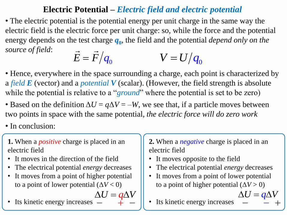
• The electric potential is the potential energy per unit charge in the same way the

electric field is the electric force per unit charge: so, while the force and the potential

energy depends on the test charge q0, the field and the potential depend only on the

source of field:

• Hence, everywhere in the space surrounding a charge, each point is characterized by

a field E (vector) and a potential V (scalar). (However, the field strength is absolute

while the potential is relative to a “ground” where the potential is set to be zero)

• Based on the definition ΔU = qΔV = –W, we see that, if a particle moves between

two points in space with the same potential, the electric force will do zero work

• In conclusion:

0V U q0qE F

Electric Potential – Electric field and electric potential

1. When a positive charge is placed in an

electric field

• It moves in the direction of the field

• The electrical potential energy decreases

• It moves from a point of higher potential

to a point of lower potential (ΔV < 0)

• Its kinetic energy increases qU V

2. When a negative charge is placed in an

electric field

• It moves opposite to the field

• The electrical potential energy decreases

• It moves from a point of lower potential

to a point of higher potential (ΔV > 0)

• Its kinetic energy increases qU V

Problem:

1. Motion of a proton in an electric field: An proton moves 2.5 cm parallel to a uniform

electric field of E = 200 N/C. Assume the electric field in the positive direction.

a) How much work is done by the field on the proton?

b) What change occurs in the potential energy of the proton?

c) What potential difference did the proton move through?

d) If the proton is released from rest what is its final speed?

• Since “everywhere in the space surrounding a charge, each point is characterized by

a field E (vector) and a potential V (scalar)”, it is natural to ask: Is there a relationship

between the two? Yes, as following:

cos cosedU dW F dx qEdxq

dU qdV

cosEdx q

0,

maxdV dV Edx

Electric Potential – Relationship between E and V

1. Consider a positive test charge q in an electric

field: since the vector electric field is tangent to the

line, the electric force on q is also tangent

2. Say that q is moved a small step dx

a) perpendicular on the field line, the field won’t do

any work:

b) parallel with the field line, the field will do a

maximum work:

electric

field line

+

E

F qEdx

0dV

maxdV

3. Therefore, the vector field is oriented such that the change in potential is maximum.

q

0dV

0dV

θ

dVE slope

dx

4. Hence, if a field is given by its position dependent potential,

and V(x) is plotted along a certain x-axis, the field in every

point is given by the negative of the slope of the V(x) graph

maxdVdU = 0 → dV = 0

dU = max → dV = max

Demonstration: for an elementary step dx in the field making an angle θ with the force

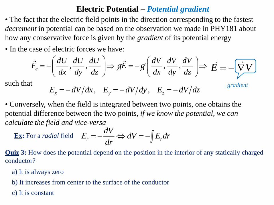
• The fact that the electric field points in the direction corresponding to the fastest

decrement in potential can be based on the observation we made in PHY181 about

how any conservative force is given by the gradient of its potential energy

• In the case of electric forces we have:

such that

, , , ,e

dU dU dU dV dV dVF qE q

dx dy dz dx dy dz

, , x y zE dV dx E dV dy E dV dz

E V

r r

dVE dV E dr

dr

Quiz 3: How does the potential depend on the position in the interior of any statically charged

conductor?

Electric Potential – Potential gradient

gradient

a) It is always zero

b) It increases from center to the surface of the conductor

c) It is constant

• Conversely, when the field is integrated between two points, one obtains the

potential difference between the two points, if we know the potential, we can

calculate the field and vice-versa

Ex: For a radial field

Electric Potential – Charged Conductors

• In the previous chapter, we learned that the electric field inside a conductor in

electrostatic equilibrium is zero. What about the electric potential?

• All points on the surface of a charged conductor in electrostatic equilibrium are at

the same potential which can be taken by convention to be zero (ground)

• A volume, or surface, or line with points at the same electric potential is called as

having an equipotential

• As shown by the relationship between E and V, the electric field at every point on

an equipotential surface is perpendicular to the surface, and the lines of electric field

are everywhere perpendicular on equipotential lines

Ex: Consider an arbitrarily shaped conductor with an excess of positive

charge in electrostatic equilibrium

• All of the charge resides at the surface, predominantly on pointier sides

• The electric field is zero inside the conductor, and nonzero and

perpendicular on the surface just outside the surface

• The electric potential is a constant everywhere on the surface of the

conductor, so no work is necessary to move charges on the surface

between any two points A and B: consistent with the fact that the field – and

so the electric force on the moving charge – is perpendicular on the surface

• The potential everywhere inside the conductor is constant and equal to its

value at the surface so the bulk is an equipotential volume

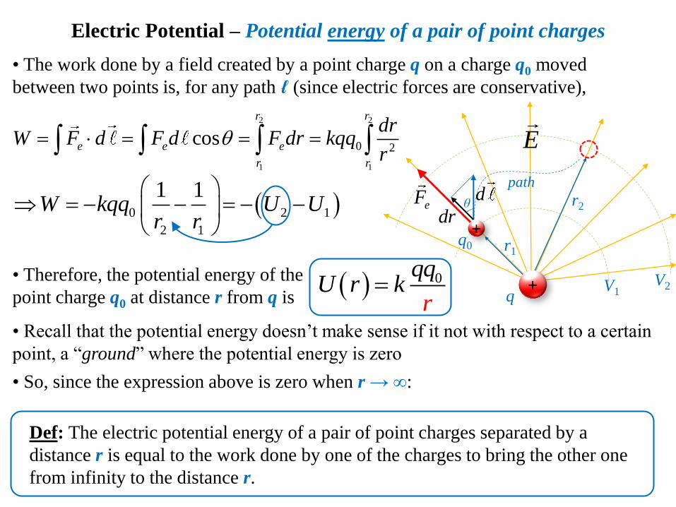
Electric Potential – Potential energy of a pair of point charges

• The work done by a field created by a point charge q on a charge q0 moved

between two points is, for any path ℓ (since electric forces are conservative),

2 2

1 1

0 2cos

r r

e e e

r r

drW F d F d F dr kqq

r

0U rr

qqk

Def: The electric potential energy of a pair of point charges separated by a

distance r is equal to the work done by one of the charges to bring the other one

from infinity to the distance r.

• Recall that the potential energy doesn’t make sense if it not with respect to a certain

point, a “ground” where the potential energy is zero

• So, since the expression above is zero when r → ∞:

• Therefore, the potential energy of the

point charge q0 at distance r from q is

0 2 1

2 1

1 1W kqq U U

r r

path

E

+

eF d

+ dr

q

q0 r1

r2

V1 V2

θ

Electric Potential – Point Source

0

U rV r k

q r

q

Comments:

• This expression gives us the work that the

field would do in order to bring a unit charge

from infinitely far away to a distance r from q

• Since it is associated with the electric field, a

potential exists at some point in space

irrespective if there is a test charge at that point

• Unlike the electric field which decreases like

1/r2, the electric potential decreases like 1/r

• A positive charge creates a positive potential

and a negative charge a negative potential

q

0

1

4 r

qV

Ex: The field strength E

in the vicinity of a

positive charge at

position r = 0 decreases

faster than the

respective potential V

relative to a point at r = ∞

V kr

q

2E k

q

r

slope of the V(r) curve for every r

+

E

+ q

r1

r2

V1 V2

1

1

qV k

r

2

2

qV k

r

• Then, based on the definition of the potential, we can

find the potential produced by a point charge source q

at a distance r, taking the ground to be at an infinite

distance from the source charge:

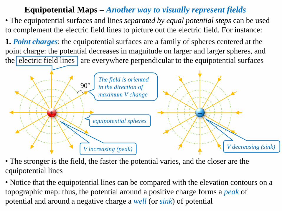
Equipotential Maps – Another way to visually represent fields

• The equipotential surfaces and lines separated by equal potential steps can be used

to complement the electric field lines to picture out the electric field. For instance:

1. Point charges: the equipotential surfaces are a family of spheres centered at the

point charge: the potential decreases in magnitude on larger and larger spheres, and

the electric field lines are everywhere perpendicular to the equipotential surfaces

90°

• The stronger is the field, the faster the potential varies, and the closer are the

equipotential lines

• Notice that the equipotential lines can be compared with the elevation contours on a

topographic map: thus, the potential around a positive charge forms a peak of

potential and around a negative charge a well (or sink) of potential

equipotential spheres

V increasing (peak) V decreasing (sink)

The field is oriented

in the direction of

maximum V change

+ –

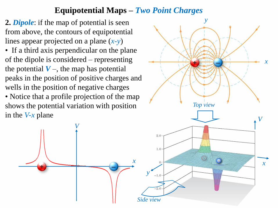
2. Dipole: if the map of potential is seen

from above, the contours of equipotential

lines appear projected on a plane (x-y)

• If a third axis perpendicular on the plane

of the dipole is considered – representing

the potential V –, the map has potential

peaks in the position of positive charges and

wells in the position of negative charges

• Notice that a profile projection of the map

shows the potential variation with position

in the V-x plane

V

x

Top view

Side view

Equipotential Maps – Two Point Charges

x

y

x

y

V

+ –

+ –

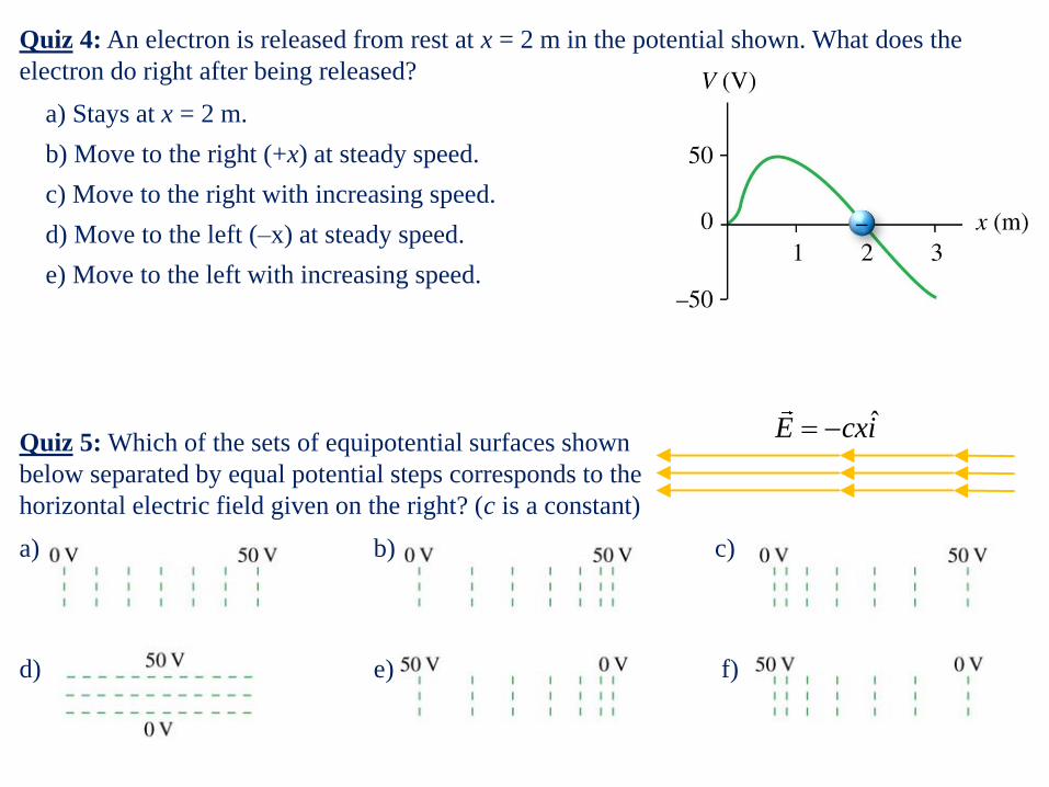
Quiz 4: An electron is released from rest at x = 2 m in the potential shown. What does the

electron do right after being released?

a) Stays at x = 2 m.

b) Move to the right (+x) at steady speed.

c) Move to the right with increasing speed.

d) Move to the left (–x) at steady speed.

e) Move to the left with increasing speed.

–

Quiz 5: Which of the sets of equipotential surfaces shown

below separated by equal potential steps corresponds to the

horizontal electric field given on the right? (c is a constant)

a) b) c)

d) e) f)

ˆE cxi

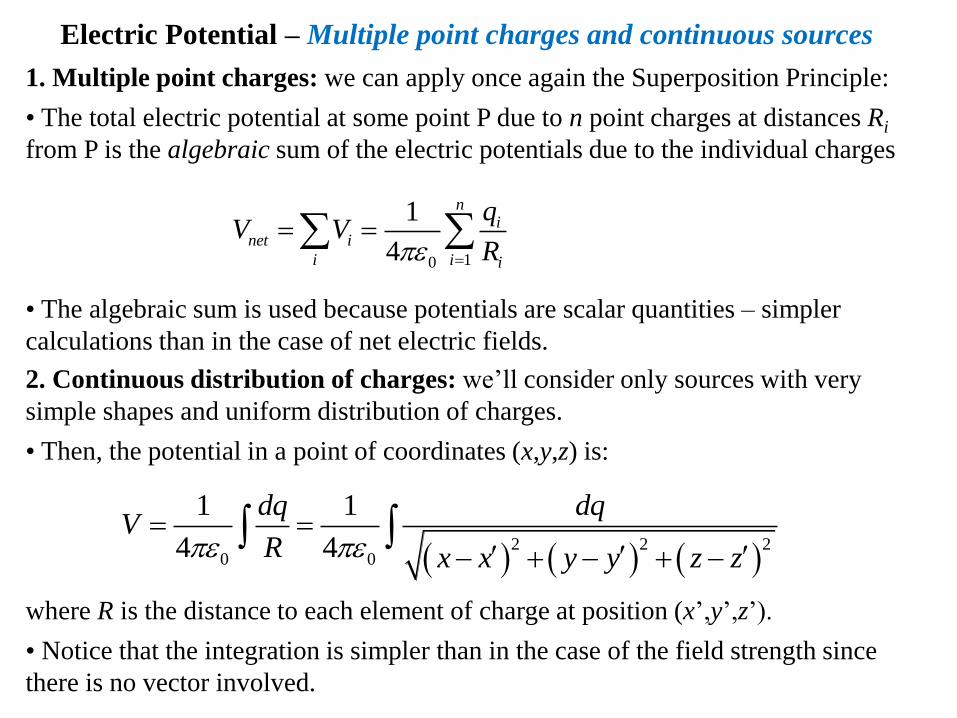
1. Multiple point charges: we can apply once again the Superposition Principle:

• The total electric potential at some point P due to n point charges at distances Ri

from P is the algebraic sum of the electric potentials due to the individual charges

• The algebraic sum is used because potentials are scalar quantities – simpler

calculations than in the case of net electric fields.

10

1

4

ni

net i

i i i

qV V

R

2. Continuous distribution of charges: we’ll consider only sources with very

simple shapes and uniform distribution of charges.

• Then, the potential in a point of coordinates (x,y,z) is:

where R is the distance to each element of charge at position (x’,y’,z’).

• Notice that the integration is simpler than in the case of the field strength since

there is no vector involved.

2 2 2

0 0

1 1

4 4

dq dqV

R x x y y z z

Electric Potential – Multiple point charges and continuous sources

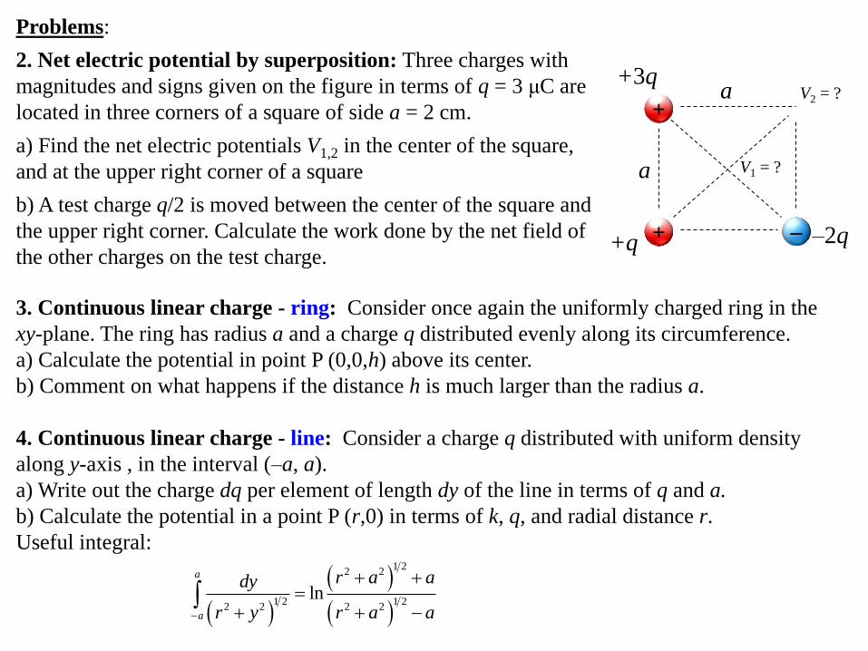
3. Continuous linear charge - ring: Consider once again the uniformly charged ring in the

xy-plane. The ring has radius a and a charge q distributed evenly along its circumference.

a) Calculate the potential in point P (0,0,h) above its center.

b) Comment on what happens if the distance h is much larger than the radius a.

4. Continuous linear charge - line: Consider a charge q distributed with uniform density

along y-axis , in the interval (–a, a).

a) Write out the charge dq per element of length dy of the line in terms of q and a.

b) Calculate the potential in a point P (r,0) in terms of k, q, and radial distance r.

Useful integral:

1 22 2

1 2 1 22 2 2 2

lna

a

r a ady

r y r a a

Problems:

2. Net electric potential by superposition: Three charges with

magnitudes and signs given on the figure in terms of q = 3 μC are

located in three corners of a square of side a = 2 cm.

a) Find the net electric potentials V1,2 in the center of the square,

and at the upper right corner of a square

b) A test charge q/2 is moved between the center of the square and

the upper right corner. Calculate the work done by the net field of

the other charges on the test charge.

a

+3q

+q –2q

a V2 = ?

– +

+

V1 = ?

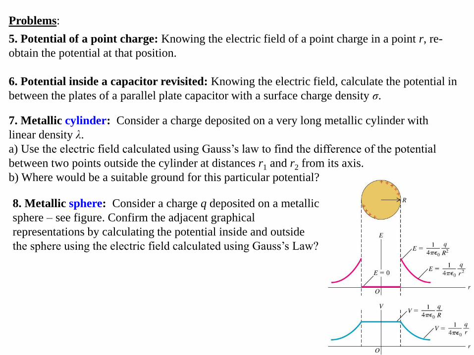
Problems:

5. Potential of a point charge: Knowing the electric field of a point charge in a point r, re-

obtain the potential at that position.

6. Potential inside a capacitor revisited: Knowing the electric field, calculate the potential in

between the plates of a parallel plate capacitor with a surface charge density σ.

8. Metallic sphere: Consider a charge q deposited on a metallic

sphere – see figure. Confirm the adjacent graphical

representations by calculating the potential inside and outside

the sphere using the electric field calculated using Gauss’s Law?

7. Metallic cylinder: Consider a charge deposited on a very long metallic cylinder with

linear density λ.

a) Use the electric field calculated using Gauss’s law to find the difference of the potential

between two points outside the cylinder at distances r1 and r2 from its axis.

b) Where would be a suitable ground for this particular potential?