Electric Energy Economics

ElectricEnergyEconomics K.E. Holbert, Sept. 2011 Page 1 of 7

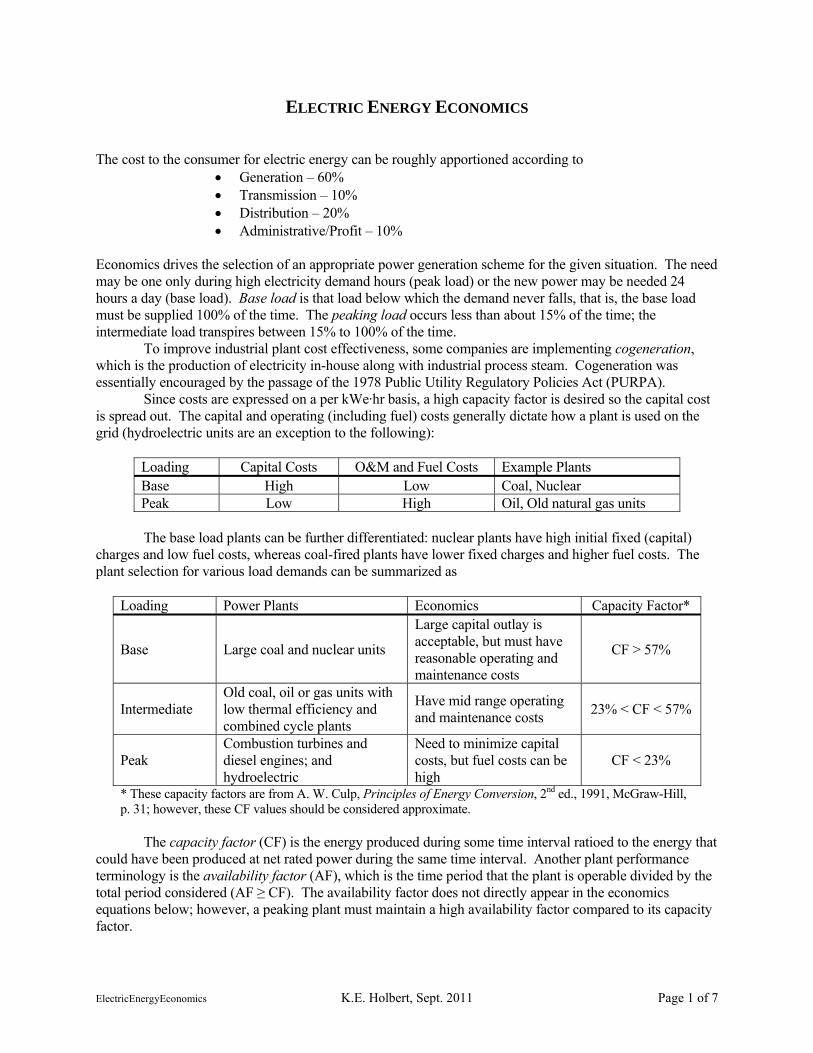
ELECTRIC ENERGY ECONOMICS The cost to the consumer for electric energy can be roughly apportioned according to

Generation – 60% Transmission – 10% Distribution – 20% Administrative/Profit – 10%

Economics drives the selection of an appropriate power generation scheme for the given situation. The need may be one only during high electricity demand hours (peak load) or the new power may be needed 24 hours a day (base load). Base load is that load below which the demand never falls, that is, the base load must be supplied 100% of the time. The peaking load occurs less than about 15% of the time; the intermediate load transpires between 15% to 100% of the time.

To improve industrial plant cost effectiveness, some companies are implementing cogeneration, which is the production of electricity in-house along with industrial process steam. Cogeneration was essentially encouraged by the passage of the 1978 Public Utility Regulatory Policies Act (PURPA).

Since costs are expressed on a per kWe·hr basis, a high capacity factor is desired so the capital cost is spread out. The capital and operating (including fuel) costs generally dictate how a plant is used on the grid (hydroelectric units are an exception to the following):

Loading Capital Costs O&M and Fuel Costs Example Plants Base High Low Coal, Nuclear Peak Low High Oil, Old natural gas units

The base load plants can be further differentiated: nuclear plants have high initial fixed (capital)

charges and low fuel costs, whereas coal-fired plants have lower fixed charges and higher fuel costs. The plant selection for various load demands can be summarized as

Loading Power Plants Economics Capacity Factor*

Base Large coal and nuclear units

Large capital outlay is acceptable, but must have reasonable operating and maintenance costs

CF > 57%

Intermediate Old coal, oil or gas units with low thermal efficiency and combined cycle plants

Have mid range operating and maintenance costs

23% < CF < 57%

Peak Combustion turbines and diesel engines; and hydroelectric

Need to minimize capital costs, but fuel costs can be high

CF < 23%

* These capacity factors are from A. W. Culp, Principles of Energy Conversion, 2nd ed., 1991, McGraw-Hill, p. 31; however, these CF values should be considered approximate.

The capacity factor (CF) is the energy produced during some time interval ratioed to the energy that

could have been produced at net rated power during the same time interval. Another plant performance terminology is the availability factor (AF), which is the time period that the plant is operable divided by the total period considered (AF ≥ CF). The availability factor does not directly appear in the economics equations below; however, a peaking plant must maintain a high availability factor compared to its capacity factor.


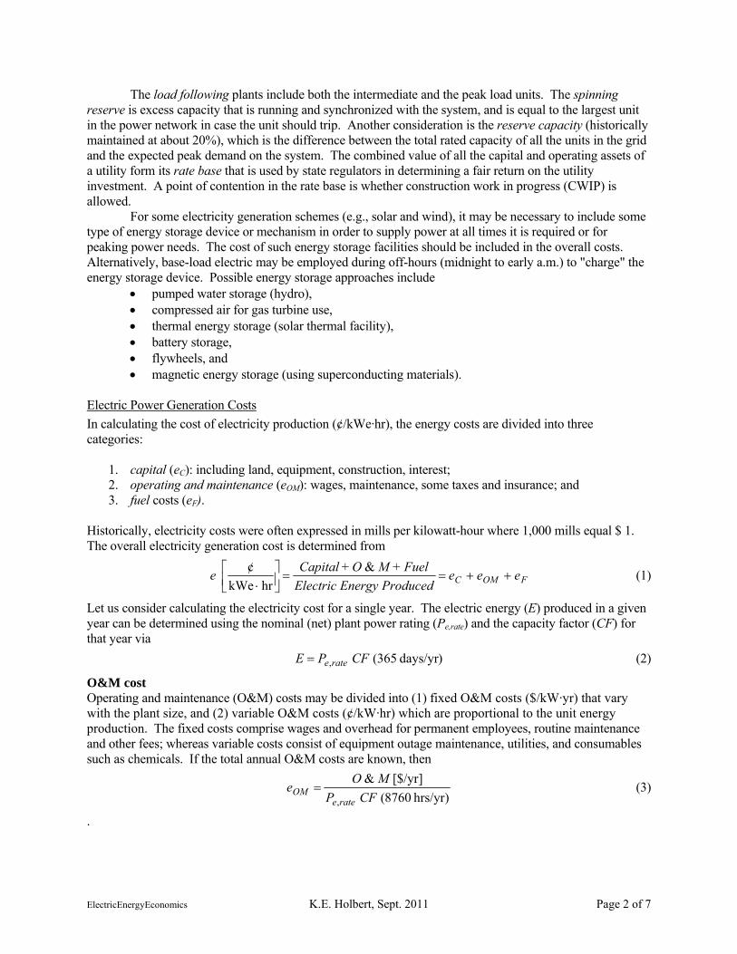
The load following plants include both the intermediate and the peak load units. The spinning reserve is excess capacity that is running and synchronized with the system, and is equal to the largest unit in the power network in case the unit should trip. Another consideration is the reserve capacity (historically maintained at about 20%), which is the difference between the total rated capacity of all the units in the grid and the expected peak demand on the system. The combined value of all the capital and operating assets of a utility form its rate base that is used by state regulators in determining a fair return on the utility investment. A point of contention in the rate base is whether construction work in progress (CWIP) is allowed.

For some electricity generation schemes (e.g., solar and wind), it may be necessary to include some type of energy storage device or mechanism in order to supply power at all times it is required or for peaking power needs. The cost of such energy storage facilities should be included in the overall costs. Alternatively, base-load electric may be employed during off-hours (midnight to early a.m.) to "charge" the energy storage device. Possible energy storage approaches include

pumped water storage (hydro), compressed air for gas turbine use, thermal energy storage (solar thermal facility), battery storage, flywheels, and magnetic energy storage (using superconducting materials).

Electric Power Generation Costs

In calculating the cost of electricity production (¢/kWe·hr), the energy costs are divided into three categories:

1. capital (eC): including land, equipment, construction, interest; 2. operating and maintenance (eOM): wages, maintenance, some taxes and insurance; and 3. fuel costs (eF).

Historically, electricity costs were often expressed in mills per kilowatt-hour where 1,000 mills equal $ 1. The overall electricity generation cost is determined from

FOMC eeeProducedEnergyElectric

Fuel + MO + Capital e

&

hrkWe

¢ (1)

Let us consider calculating the electricity cost for a single year. The electric energy (E) produced in a given year can be determined using the nominal (net) plant power rating (Pe,rate) and the capacity factor (CF) for that year via

)days/yr365(, CFPE ratee (2)

O&M cost Operating and maintenance (O&M) costs may be divided into (1) fixed O&M costs ($/kW·yr) that vary with the plant size, and (2) variable O&M costs (¢/kW·hr) which are proportional to the unit energy production. The fixed costs comprise wages and overhead for permanent employees, routine maintenance and other fees; whereas variable costs consist of equipment outage maintenance, utilities, and consumables such as chemicals. If the total annual O&M costs are known, then

)hrs/yr 8760(

]$/yr[&

, CFP

MOe

rateeOM (3)

.


Example: Consider a hypothetical 600 MWe power plant, whose operating costs are purely due to the salaries of the dozen workers employed there. If the annual wages and overhead average $100,000 per employee, and the capacity factor is 35%, what is the O&M component of the electricity cost?

hrmills/kWe·65.0)hrs/yr8760)(35.0)(kW10600(

)mills/$1000)(/yr000,100)($employees12(3

OMe

Clearly, this example lacks consideration of all the various O&M costs. Fuel cost The fuel cost is probably the next easiest component to determine. The annual thermal heat required to produce a given amount of electricity can be determined from the plant thermal efficiency. The thermal

efficiency (ηth) is the net electricity generated (Pe) divided by the heat input ( thQ ) required to produce that

electricity, i.e., theth QP . The thermal heat produced is the product of the fuel input rate ( fuelm ) and

the fuel heat content (e.g., heating value, HV), that is, HVmQ fuelth . The annual electric energy

produced, with some representative units for the various quantities, is thus

Btu/kJ

hrkWeton/galBtu/kJ

yrton/gal

yrhrkWe

thfuel HVmE (4)

The annual fuel cost is determined from the amount (e.g., mass or volume) of fuel used and its cost per unit mass or volume (FC)

ton/gal

$yr

ton/galyr$

Cfuel FmFuel (5)

For a fossil-fired unit, FC is commonly expressed in terms of dollars per ton or gallon, and the heating value is given in Btu/lbm or Btu/gal. For a nuclear power plant, FC is typically quoted in dollars per kilogram of uranium, and the burnup, B in MWth·day per metric ton of uranium (MTU), is the terminology employed for expressing fuel heat content. By combining the above two expressions, we arrive at the fuel cost of electricity

th

CF HV

F

E

Fuele

(6)

As should be expected, the fuel cost is independent of the plant capacity factor. Example: An 800 MWe coal-fired unit has a thermal efficiency of 38% and a capacity factor of 82%. The utility is in negotiations for a long-term contract for coal having a heating value of 15,700 Btu/lbm. To hold the fuel cost below 0.9 ¢/kWe·hr, what is the maximum price, in dollars per short ton, that the utility should be willing to pay?

ton/47.31$2000)38.0(700,159.0¢100

$1tonlbm

Btu3412kW·hr1

lbmBtu

kW·hr¢ thFC HVeF

The given capacity factor was extraneous information. Capital cost Computation of the capital cost is the most difficult due to the large expenditure and time period involved. As a substantial simplification, the capital cost can be likened to a home mortgage payment, which mostly consists of principal and interest. Significant differences between the home mortgage and power plant cases do exist however. For example, power plants take years (vs. months) to build; hence, utilities must borrow money during the plant construction period (granted some individuals obtain home construction


loans too). In addition, the time value of money should be considered, that is, the value of one dollar ten years from now will likely be different than today, and depreciation should also be accounted for.

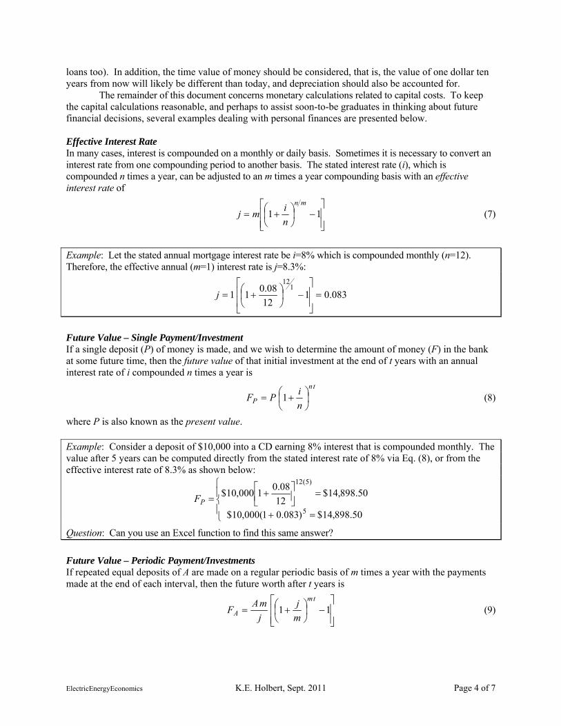
The remainder of this document concerns monetary calculations related to capital costs. To keep the capital calculations reasonable, and perhaps to assist soon-to-be graduates in thinking about future financial decisions, several examples dealing with personal finances are presented below. Effective Interest Rate In many cases, interest is compounded on a monthly or daily basis. Sometimes it is necessary to convert an interest rate from one compounding period to another basis. The stated interest rate (i), which is compounded n times a year, can be adjusted to an m times a year compounding basis with an effective interest rate of

11

mn

n

imj (7)

Example: Let the stated annual mortgage interest rate be i=8% which is compounded monthly (n=12). Therefore, the effective annual (m=1) interest rate is j=8.3%:

083.0112

08.011

112

j

Future Value – Single Payment/Investment If a single deposit (P) of money is made, and we wish to determine the amount of money (F) in the bank at some future time, then the future value of that initial investment at the end of t years with an annual interest rate of i compounded n times a year is

tn

P n

iPF

1 (8)

where P is also known as the present value. Example: Consider a deposit of $10,000 into a CD earning 8% interest that is compounded monthly. The value after 5 years can be computed directly from the stated interest rate of 8% via Eq. (8), or from the effective interest rate of 8.3% as shown below:

50.898,14$)083.01(000,10$

50.898,14$12

08.01000,10$

5

)5(12

PF

Question: Can you use an Excel function to find this same answer?

Future Value – Periodic Payment/Investments If repeated equal deposits of A are made on a regular periodic basis of m times a year with the payments made at the end of each interval, then the future worth after t years is

11

tm

A m

j

j

mAF (9)


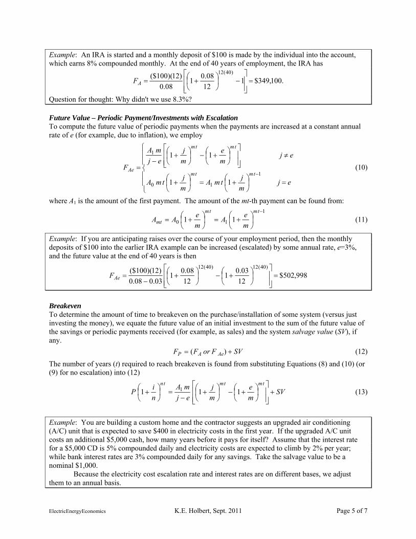
Example: An IRA is started and a monthly deposit of $100 is made by the individual into the account, which earns 8% compounded monthly. At the end of 40 years of employment, the IRA has

.100,349$112

08.01

08.0

)12)(100($)40(12

AF

Question for thought: Why didn't we use 8.3%? Future Value – Periodic Payment/Investments with Escalation To compute the future value of periodic payments when the payments are increased at a constant annual rate of e (for example, due to inflation), we employ

ejm

jtmA

m

jtmA

ejm

e

m

j

ej

mA

Ftmtm

tmtm

Ae1

10

1

11

11

(10)

where A1 is the amount of the first payment. The amount of the mt-th payment can be found from:

1

10 11

tmtm

mt m

eA

m

eAA (11)

Example: If you are anticipating raises over the course of your employment period, then the monthly deposits of $100 into the earlier IRA example can be increased (escalated) by some annual rate, e=3%, and the future value at the end of 40 years is then

998,502$12

03.01

12

08.01

03.008.0

)12)(100($)40(12)40(12

AeF

Breakeven To determine the amount of time to breakeven on the purchase/installation of some system (versus just investing the money), we equate the future value of an initial investment to the sum of the future value of the savings or periodic payments received (for example, as sales) and the system salvage value (SV), if any.

SVForFF AeAP )( (12)

The number of years (t) required to reach breakeven is found from substituting Equations (8) and (10) (or (9) for no escalation) into (12)

SVm

e

m

j

ej

mA

n

iP

tmtmtn

111 1 (13)

Example: You are building a custom home and the contractor suggests an upgraded air conditioning (A/C) unit that is expected to save $400 in electricity costs in the first year. If the upgraded A/C unit costs an additional $5,000 cash, how many years before it pays for itself? Assume that the interest rate for a $5,000 CD is 5% compounded daily and electricity costs are expected to climb by 2% per year; while bank interest rates are 3% compounded daily for any savings. Take the salvage value to be a nominal $1,000. Because the electricity cost escalation rate and interest rates are on different bases, we adjust them to an annual basis.


03045.01365

03.01105127.01

365

05.011

1365

1365

ji

We employ Eq. (13) to determine the breakeven point

000,1$)02.1()03045.1(51.277,38$)05127.1(000,5$

)000,1($1

02.01

1

03045.01

02.003045.0

)1()400($

1

05127.01)000,5($

)1()1()1(

ttt

ttt

Numerical solution of the above equation shows that the system starts to pay for itself in the twentieth year after purchase. Question: do you think the A/C unit will last 20 years? Present Value – Uniform Series For a present value (loan amount) of PA, the periodic payment (A) can be determined from

tn

A n

i

i

nAP 11 (14)

Example: What is the monthly principal and interest payment for a $100,000 loan borrowed over 30 years at an 8% interest rate?

month/76.733$12

08.011

08.0

12.000,100$

)30)(12(

AA

This same value is found in Excel using ‘PMT(8%/12,360,100000,0)’. Question: what is the total amount paid over the loan period? The capital (or fixed) cost must be properly distributed throughout the expected operating lifetime of the plant. For financial analyses, plants are generally assumed to have a lifetime of 40 years, although they may operate for either a shorter or a longer period. If the utility spreads the construction costs and interest over 40 years with equal annual (or monthly) payments, then our objective is to find the annual payment amount. To do so, we can think of the payment as being some percentage of the construction cost (FB), that is, we can establish a levelized annual fixed-charge rate (I) such that

8760)hrs/yr 8760(hrkWe

¢

,, CF

I

P

F

CFP

F I

E

CAP e

ratee

B

ratee

BC

(15)

where CAP is the annualized amount of the entire capital costs including interest. The term rateeB PF ,/ is

the cost of building a power plant, which is generally expressed in terms of dollars per installed kilowatt-electric ($/kWe). As the electric rating is increased, the ratio rateeB PF ,/ generally decreases—this is

known as economy of scale. Table I shows representative production costs for electric generating stations in the U.S. Example: A 500-MW power plant costs $ 1,200 per kWe. If the expected capacity factor is 87%, determine the appropriate annual fixed-charge rate (I) and the capital cost of the electricity. First, determine the initial cost to build the power plant

million 600$)kWe/200,1)($kWe10500( 3 BF


Next, make a simple determination of the annual payment for principal and interest using Eq. (14) and assuming a 5% interest rate paid over 40 years:

CAPAA

million/yr967.34$1

05.011

05.0

1million 600$

)40)(1(

From Eq. (15), the levelized annual fixed-charge rate is

yr/%83.5%)100(million 600$

million/yr 967.34$

BF

CAPI

Finally, the capital portion of the electricity cost is

/kWe·hr¢918.01$

¢ 100

hr/yr) 0(0.87)(876

yr/0583.0

kWe

200,1$

8760,

CF

I

P

Fe

ratee

BC

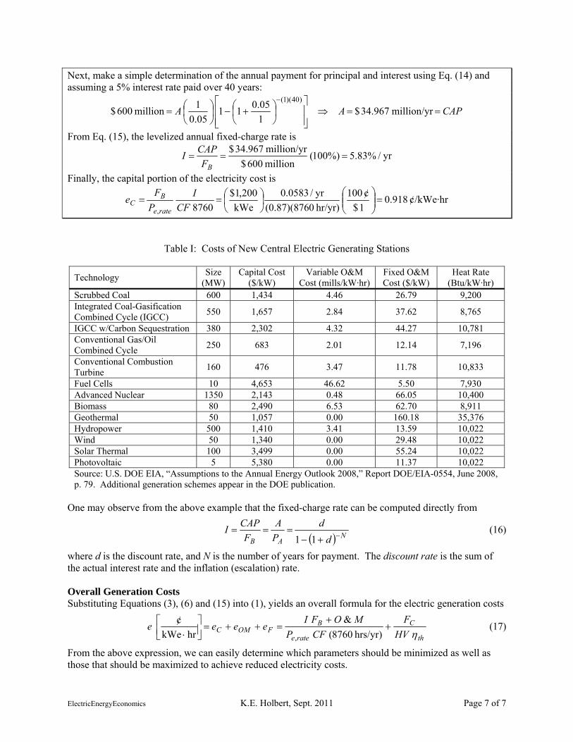
Table I: Costs of New Central Electric Generating Stations

Technology Size

(MW) Capital Cost

($/kW) Variable O&M

Cost (mills/kW·hr) Fixed O&M Cost ($/kW)

Heat Rate (Btu/kW·hr)

Scrubbed Coal 600 1,434 4.46 26.79 9,200 Integrated Coal-Gasification Combined Cycle (IGCC)

550 1,657 2.84 37.62 8,765

IGCC w/Carbon Sequestration 380 2,302 4.32 44.27 10,781 Conventional Gas/Oil Combined Cycle

250 683 2.01 12.14 7,196

Conventional Combustion Turbine

160 476 3.47 11.78 10,833

Fuel Cells 10 4,653 46.62 5.50 7,930 Advanced Nuclear 1350 2,143 0.48 66.05 10,400 Biomass 80 2,490 6.53 62.70 8,911 Geothermal 50 1,057 0.00 160.18 35,376 Hydropower 500 1,410 3.41 13.59 10,022 Wind 50 1,340 0.00 29.48 10,022 Solar Thermal 100 3,499 0.00 55.24 10,022 Photovoltaic 5 5,380 0.00 11.37 10,022 Source: U.S. DOE EIA, “Assumptions to the Annual Energy Outlook 2008,” Report DOE/EIA-0554, June 2008, p. 79. Additional generation schemes appear in the DOE publication.

One may observe from the above example that the fixed-charge rate can be computed directly from

N

AB d

d

P

A

F

CAPI

11 (16)

where d is the discount rate, and N is the number of years for payment. The discount rate is the sum of the actual interest rate and the inflation (escalation) rate. Overall Generation Costs Substituting Equations (3), (6) and (15) into (1), yields an overall formula for the electric generation costs

th

C

ratee

BFOMC HV

F

CFP

MOFIeee e

)hrs/yr 8760(

&

hrkWe

¢

,

(17)

From the above expression, we can easily determine which parameters should be minimized as well as those that should be maximized to achieve reduced electricity costs.

Documents

Electric Energy Economics