Electoral Rules and Corruption - Home | Projects at …projects.iq.harvard.edu/gov2126/files/person_tabellini...ELECTORAL RULES AND CORRUPTION Torsten Persson Stockholm University

ELECTORAL RULES AND CORRUPTION

Torsten PerssonStockholm University

Guido TabelliniBocconi University

Francesco TrebbiHarvard University

AbstractIs corruption systematically related to electoral rules? Recent theoretical work suggests apositive answer. But little is known about the data. We try to address this lacuna by relatingcorruption to different features of the electoral system in a sample of about eighty democ-racies in the 1990s. We exploit the cross-country variation in the data, as well as the timevariation arising from recent episodes of electoral reform. The evidence is consistentwith thetheoretical priors. Larger voting districts—and thus lower barriers to entry—are associatedwith less corruption, whereas larger shares of candidates elected from party lists—and thusless individualaccountability—are associatedwith more corruption. Individualaccountabilityappears to be most strongly tied to personal ballots in plurality-rule elections, even thoughopen party lists also seem to have some effect. Because different aspects roughly offset eachother, a switch from strictly proportional to strictly majoritarian elections only has a smallnegative effect on corruption. (JEL: E62, H3)

1. IntroductionElected politicians have ample opportunity to abuse their political powers at theexpense of voters. Corruption— or, more generally, extraction of politicalrents—is not only a problem in developing and young democracies, but also indeveloped and mature ones. Moreover, available measures indicate that theincidence of corruption varies substantially among countries with similar eco-nomic and social characteristics. As voters can hold their elected representativesaccountable at the polls, it is natural to ask whether different electoral rules workmore or less well in imposing accountability on incumbent politicians. Indeed,

Acknowledgments: We are grateful to seminar participants and John Carey, Francesco Corielli,Elhanan Helpman, Andrea Ichino, Costas Meghir, David Stromberg, Jakob Svensson, and twoanonymous referees for helpful comments. We thank Alessandra Bon� glioli, Agostino Consolo,and Jose Maurico Prado Jr. for research assistance and Christina Lonnblad for editorial assistance.Financial support was given by the European Commission (a TMR grant), MURST, BocconiUniversity and the Swedish Research Council.E-mail addresses: Persson: [email protected]; Tabellini: [email protected];Trebbi: [email protected].

© 2003 by the European Economic Association

perceptions among voters of widespread abuses of power by the ruling politicalelite were a major factor behind the electoral reforms in Italy and Japan duringthe mid-1990s.

Are political rents systematically related to electoral rules? A few theoret-ical studies have addressed this important issue. We describe the main ideasbehind existing theoretical models in Section 2. Brie� y, the theory identi� esthree critical aspects of the electoral system: (1) the ballot structure, (2) districtmagnitude, and (3) the electoral formula. With regard to (1), some electoralsystems make incumbents individually accountable to the voters, while otherselect politicians from party lists. A party-list system weakens individual incen-tives for good behavior, because it creates free-rider problems and more indirectchains of delegation, from voters to parties to politicians. As for (2), fewerlegislators elected in a typical electoral district (low district magnitude) mayincrease corruption because it raises barriers to entry. A smaller number ofparties (or ideological types) present themselves at the polls and voters have lessopportunity to oust corrupt politicians or parties. When it comes to (3), theelectoral formula may also shape rent extraction through the sensitivity ofelection outcomes to incumbent performance. Since incumbents may be moreseverely punished under plurality rule than under proportional representation(PR), the former may be more effective in deterring corruption.

A number of empirical studies have tried to uncover economic and socialdeterminants of corruption: we outline some of their results in Section 3, whendescribing our data. But the question of how electoral rules correlate withcorruption in a large cross section of countries still remains unanswered.1 Tryingto � ll this lacuna in the literature, we relate corruption to electoral rules assuggested by theory in a sample from the 1990s encompassing data from about80 democracies. We use several indicators of rent extraction, measuring per-ceptions of the degree of corruption by public of� cials and ineffectiveness in thedelivery of government service. The perceptions are those of business people,risk analysts and the general public.

We present results for alternative measures obtained by alternative methods.Section 4 � rst provides results from conventional cross-sectional estimates,where we try to identify the effect of different aspects of the electoral system.Recognizing that independent and dependent variables may be measured witherror, we report on sensitivity analysis where political rents and electoral rulesare measured in alternative ways. But drawing inferences from cross-sectionalestimates is dif� cult, because omitted-variable bias is always possible. Based onthe electoral reforms occurring in the 1990s, we also report on panel estimatesexploiting time variation in the perceptions of corruption. We also brie� y

1. In a recent paper, Kunicova and Rose-Ackerman (2002) investigate the effect of the politicalconstitution on perceptions of corruption in a large cross section of countries. They emphasize therole of party selection of candidates and contrast electoral systems with closed and open lists. Their� nding (that closed list systems are associated with more corruption) is consistent with ourempirical results.

959Persson et al. Electoral Rules and Corruption

discuss the empirical results presented in Persson, Tabellini, and Trebbi (2002)and Persson and Tabellini (2003): a binary classi� cation of electoral formulasallows these to take into account possible selection bias and nonlinearities—such as heterogeneous effects of electoral rules on corruption, depending on thecultural or historical environment.

Our results suggest that the details of electoral rules have a strong in� uenceon political corruption. Consistent with the theoretical hypothesis on the ballotstructure, corruption is higher the larger is the fraction of candidates elected onparty lists. The combination of individual ballots and plurality rule seems themost effective in reducing corruption, but open-lists systems under PR (wherevoters may express preferences for certain names on the list) also appear toreduce corruption. Consistent with the hypothesis on district magnitude, andcontrolling for the ballot structure, corruption is also higher in countries electingfewer candidates per district. As systems based on PR electoral formulas tend tocombine large district magnitude and citizens casting their ballot for party lists,while plurality systems tend to have small districts where citizens cast theirballot for individuals, however, corruption may not change much across a crudeclassi� cation of electoral systems.

2. Theory

What can economic and political theory say about the mapping from theelectoral rule to corruption or rents for politicians? Some recent analyticalstudies have addressed this question.

One idea is that electoral rules promoting the entry of many parties orcandidates reduce rents captured by politicians. The clearest formalization isperhaps that in Myerson (1993). He assumes that parties (or equivalently,candidates) differ in two dimensions: their intrinsic honesty and their ideology.All voters prefer honest candidates but disagree on ideology. Dishonest incum-bents may still cling on to power if voters sharing the same ideologicalpreferences cannot � nd a good substitute candidate. The availability of goodcandidates depends on district magnitude. With PR and large districts (meaningthat several candidates can be elected in each district), an honest candidate isalways available, for all ideological positions. Dishonest candidates thus haveno chance of being elected in equilibrium. But in single-member districts, theequilibrium can be very different. Even if honest candidates run for of� ce for allpossible types of ideology, only one candidate can win the election. This impliesthat voters vote strategically, and may vote for the dishonest but ideologicallypreferred candidate if they expect all other voters with the same ideology to dothe same. Switching to the honest candidate risks giving the victory to acandidate on the other side of the ideological scale. In other words, small districtmagnitude together with strategic voting increases the barriers to entry in the

960 Journal of the European Economic Association June 2003 1(4):958 –989

electoral system, and makes it more dif� cult to oust dishonest incumbents fromof� ce.

In Myerson’s model, voting behavior is endogenous to the electoral rule,whereas dishonesty is an exogenous feature of candidates. Ferejohn (1986)instead endogenizes the behavior of incumbents, by letting them choose a levelof effort, given that voters hold incumbents accountable for their performancethrough a retrospective-voting rule. As shown by Persson, Roland, and Tabellini(2000), one can easily reformulate Ferejohn’s model such that rent extraction isequivalent to exerting little effort, and other papers have used Ferejohn’s modelto analyze the determinants of corruption (e.g., Adsera, Boix, and Payne 2000).In Ferejohn’s model, electoral defeat is less fearsome the higher is the proba-bility of an ousted incumbent returning to of� ce in the future. While Ferejohntreats this probability as an exogenous parameter, he points out that it is likelyto be negatively related to the number of parties, or the number of candidates.This brings us back to the barriers of entry raised by the electoral system.

To summarize, these analyses predict that voting in single-member constit-uencies is less effective in containing corruption, compared to electoral systemswith large districts. District magnitude and thresholds for representation are thecritical features of the electoral system. Larger electoral districts and lowerthresholds imply lower barriers to entry, and thus lead to less corruption andlower rents for politicians.

But electoral systems differ in two other important dimensions, namely inthe electoral formula translating vote shares into seat shares, and in the ballotstructure. Plurality rule awards the seats in an M seat district to the individualcandidates receiving the M highest vote shares. Under PR, voters instead chooseamong party lists and the number of candidates elected from each list dependson the vote share of each party. Moreover, different electoral systems affordvoters different degrees of choice over the candidates nominated on each list.

Persson and Tabellini (2000, Ch. 9), building on the career-concern modelof Holmstrom (1982), suggest a model of rents and corruption resting preciselyon these differences in the ballot structure associated with plurality and PRsystems. The main idea is that voting over individual candidates creates a directlink between individual performance and reappointment. Individuals havestrong incentives to perform well in of� ce, by exerting effort or avoiding abuseof power. When voters choose among party lists, politicians’ incentives areinstead diluted by two effects. First, a free-rider problem arises among politi-cians on the same list. The reason is that under PR, the number of seats dependson the votes collected by the whole list, rather than the votes for each individualcandidate. Second, if the list is closed and voters cannot choose their preferredcandidate, an individual’s chance of re-election depends on his rank on the list,not his individual performance. If lists are drawn up by party leaders (as iscommonly the case), the ranking is likely to re� ect criteria unrelated to com-petence in providing bene� ts to voters, such as party loyalty, or effort within theparty (rather than in of� ce). Then, individual incentives to perform well are


much weaker. Persson and Tabellini’s analysis therefore predicts political rentsand corruption to be higher, the lower is the proportion of representativeselected via individually assigned seats, rather than party lists. Implicitly, their sresults also suggest that rents ought to be higher if the list is closed (i.e., votershave no choice over the ranking of individual candidates on the list) than if it isopen.2

Finally, Persson and Tabellini (1999) suggest another mechanism wherebythe electoral system may affect rent extraction. Their model studies electoralcompetition in two stylized systems: a “proportional system” with PR in a singlenation-wide district, and a “majoritarian system” with plurality rule in severalsingle-member districts. Electoral competition is stiffer in the latter, as candi-dates are induced to focus their attention on winning a majority, not in thepopulation at large, but in “marginal districts” containing a large number ofswing voters. As these voters are more willing to switch their votes in responseto policy, candidates become more disciplined and extract less equilibriumrents. This prediction is somewhat imprecise on the critical features of theelectoral system, in that the argument does not distinguish well between districtmagnitude and the electoral formula. But a similar distinction between majori-tarian and proportional elections is a general and widespread idea in the politicalscience literature.3 This literature emphasizes the idea that the electoral outcomeis more sensitive to the performance of the incumbent under majoritarianelections. Sometimes, this is attributed to the fact that this electoral rule is lesslikely to lead to coalition governments (and that voters � nd it more dif� cult toidentify who is responsible for disappointing performance in coalition thansingle-party governments). Alternatively, it is argued that swings in vote shareshave much more drastic consequences for seat shares and the electoral outcomeunder majoritarian than under proportional elections.4

Summarizing, the hypothesis we would ideally want to take to the data canbe stated as follows:

2. Carey and Shugart (1995) have suggested that the ballot structure is important for yet anotherreason. In some open-list systems, as well as the SNTV, candidates compete to win preferencevotes against other candidates belonging to the same party. This kind of intraparty competition mayinduce more (rather than less) corruption. One reason is that candidates offer personal favors tovoters (e.g., in� uence in speci� c public sector activities). A second reason is that they may needto raise additional electoral � nancing—perhaps through illegal means. At the core of this idea liesan implicit distinction between intraparty and interparty competition. Interparty competition isgood for voters, because it encourages politicians to produce good legislation and good policies;intraparty competition is bad, because it may encourage illegal behavior and thus, promotecorruption. Reed and Thies (2001) suggest that one motive behind the recent electoral reforms inJapan was to eliminate this kind of undesirable intraparty competition. In this paper, we do notinvestigate the empirical validity of this idea. But Golden and Chang (2000) � nd support for it inan empirical study of the Italian Christian Democrats.3. For example, such a distinction � gures prominently in the well-known work by Lijphart (1994,1999) and Powell (2000).4. PR makes vote and seat shares proportional almost by de� nition. But with plurality andsingle-member constituencies, the seat share changes much more rapidly with the vote share, aphenomenon often refereed to as the “cube law” in the comparative-politics literature.


H1: Larger district magnitude and lower thresholds for representation shouldbe associated with less corruption (the barriers-to-entry effect).H2: A larger share of representatives elected on an individual ballot, ratherthan on party lists, should be associated with less corruption (the career-concern effect).H3: Plurality rule in small districts should be associated with less corruptionthan PR in large districts (the electoral-competition effect).

These theoretical predictions are complementary, in the sense of each modelemphasizing a different mechanism, and more than one of them can be consis-tent with the same data. For example, Persson and Tabellini (1999) take thenumber of parties/candidates as given and do not consider the incentives ofindividual politicians.

Moreover, our three predictions concern the effects of combinations of thethree main features of real world electoral systems, namely: (1) district magni-tude, (2) ballot structure, and (3) the electoral formula. H2 e.g., relies on a modeldistinguishing between different electoral systems on the basis of both (2) and(3), while H3 relies on a model making a distinction in terms of (1) and (3).

Finally, district magnitudes, ballot structures and electoral formulas are notindependent features of real-world electoral rules, but combined in a systematicpattern. Countries with “majoritarian electoral systems” typically combine sin-gle-member districts and plurality rule where voters select individual candidates(as the archetypal British � rst-past-the-post system). At the opposite extreme,many “proportional systems” indeed have large districts and PR, where voterschoose among party lists (Israel e.g., has just one nationwide district where all120 representatives are elected via party lists).5

Because of these correlations, precise empirical testing of the three hypoth-eses is not a trivial task. We discuss our empirical strategy in Section 4. Beforethat, however, we turn to the question of how to measure the relevant aspects ofelectoral rules in a sample of contemporary democracies.

3. Data

We now turn to a discussion of the key variables used in the empirical analysis.These data have been collected as part of a larger research program on economicpolicy and comparative politics. The Data Appendix gives a succinct descriptionof the data sources, while Persson and Tabellini (2003) provide a more com-prehensive discussion.

5. Cox (1997), as well as Blais and Masicotte (1996), give recent overviews of the electoralsystems across the world’s democracies.


3.1 Electoral Rules and Political Institutions

Our sample consists of about 80 democracies in the 1990s. To de� ne ademocracy we rely on the surveys published by Freedom House. The so-calledGastil indexes of political rights and civil liberties, respectively, vary on adiscrete scale from 1 to 7, with low values associated with better democraticinstitutions. For the countries included in our default sample, the average ofthese two indexes (GASTIL) in the period 1990 –98 does not exceed 5. Tomaximize the number of countries, we adopt a generous de� nition of democ-racy, which includes countries such as Zimbabwe (although the main deterio-ration of democratic rights occurred after 1998). But we also report results fora more narrow sample of better democracies, with an average score of less than3.5 in the 1990 –1998 period.

The countries in our sample also differ in how long they have beendemocracies. This could matter: older democracies might have a better systemof checks and balances to � ght corruption and the abuse of power. For thisreason, we record the age of each democracy (AGE), de� ned as the fraction oftime of uninterrupted democratic rule going back in time (for a maximum of 200years) from the current date until the date of � rst becoming an independentdemocracy. In the empirical work, we always control for both the quality (asmeasured by GASTIL) and age (as measured by AGE) of the democracy.

How do we measure the different aspects of electoral rules, given thetheoretical predictions summarized in the previous section? To test the barriers-to-entry effect (H1 in Section 2), we measure the average magnitude of votingdistricts (MAGN), de� ned as the number of districts (primary as well assecondary or tertiary, if applicable) divided by the number of seats in the lowerhouse. Thus, MAGN is the inverse of district magnitude as commonly de� ned bypolitical scientists; it ranges between 0 and 1, taking a value of 1 in a UK-stylesystem with single-member districts and a value close to 0 in an Israel-stylesystem with a single national district. Its expected effect on corruption ispositive, according to H1.

In some cases, we also rely on an alternative measure of district magnitudecollected and discussed by Seddon, Gaviria, Panizza, and Stern (2001). Theirvariable PDM is de� ned as traditional measures of district magnitude (i.e., asseats over districts), except that district magnitude is now a weighted average,where the weight on each district magnitude in a country is the share oflegislators running in districts of that size. We use the measure provided bySeddon et al. (2001) as is, except that we divide it by 100 so as to constrain itsvalue to the (0, 1) range. This variable has an expected negative effect oncorruption.

The career-concern effect (H2 in Section 2) instead focuses on the ballotstructure and, indirectly, on the electoral formula. Here, the empirical counter-part to the theory is somewhat less straightforward. The theory identi� es two(related) effects on corruption, due to party lists rather than individual ballots.


The � rst is the free-rider problem among politicians on the same list. The secondis the effect of a closed list (where the ranking of candidates on the list ispredetermined and cannot be changed by voters). To capture these two differenteffects, we use two alternative continuous measures of the ballot structure.

The � rst and stricter measure, called PINDP, is designed to re� ect the free-ridereffect only. It is thus de� ned as the proportion of legislators in the lower house whoare elected on an individual ballot by plurality rule. All individuals elected via partylists are lumped together and coded as 0, irrespective of whether the list is open orclosed, since they are all affected by the free-rider problem. Thus, this variable takesa value of 1 in the UK (where all legislators are elected by individual votes underplurality rule), a value of approximately 0.5 in Germany (where only about half thelegislators are elected in that way), and a value of 0 in Poland (where all legislatorsare elected via party lists, even though voters’ preferences determine the whichcandidates on the list get elected). Its expected effect on corruption is negative,according to H2.6

The second measure, called PINDO, is designed to re� ect the effect of closedlists only. It is de� ned as the proportion of legislators in the lower house electedindividually or on open lists. The legislators elected in closed lists are instead codedas 0. This different de� nition of individual accountability discriminates betweenballots where voters choose among individuals and those where they do not,irrespective of whether there is a free-rider problem. By this measure, the UK is stillcoded as 1 and Germany as 0.5, but now Poland (with open lists) is coded as 1. Thevariables PINDP and PINDO take on different values in thirteen countries: thoseusing a semi-proportional STV-system, plus those where voters must vote forindividual politicians in open-list or panachage systems. For this variable as well,the expected effect on corruption is negative, according to H2.7

Also on this feature of the electoral rule, we refer to an alternative variablecompiled by Seddon et al. (2001): it is called PPROPN and measures the shareof legislators elected in national (secondary or tertiary) districts rather thansub-national (primary) districts. As the emphasis on collective vs. individual

6. This de� nition still gives rise to a few borderline cases. Thus, we classify the SNTV systemused for the lower houses in Taiwan (part of the house) and Japan (before the mid-1990s reform)as individual voting under plurality rule and set PINDP 5 1. The hybrid system in Chile formallyhas party lists in two-member districts. But the seats are won based on individual votes (open list),and the system has plurality in the sense that a � rst-ranked list that collects more than twice thenumber of votes as a second-ranked list wins both the seats in a district. We treat also this case asplurality rule on individual ballots and set PINDP 5 1.7. Party-list voting can be of three types: closed lists, open lists (or preference vote), andpanachage. Closed lists do not allow voters to express a preference for individual candidates, so weset PINDO 5 0. A preference vote on open lists may be prescribed (as in Finland), or allowed (asin Sweden) with the party list still being the default option for the vector. We code as PINDO 51 only those systems where the ranking on the party lists is exclusively decided by the preferentialvotes (Brazil, Cyprus, Estonia, Finland, Greece, (prereform) Italy, Poland, Slovakia, and SriLanka). Among other PR-systems, the panachage (used in Luxembourg and Switzerland) alsogives voters the option of expressing preferences across parties. Here, we set PINDO 5 1. Finally,the PR system in Ireland is not based on party lists, but on the Single Transferable Vote, which isalso used in Malta. In these cases too, we set PINDO 5 1.


accountability may be largest for a politician running on a national party list, wesometimes use PPROPN as an alternative to PINDP or PINDO. The expectedsign of this variable is positive (since it is de� ned in the opposite way relativeto PINDP and PINDO).

Finally, the electoral competition effect (H3 in Section 2) refers to a discon-tinuous change in both district magnitude and the electoral formula. When takingthis hypothesis to the data, we classify electoral systems into “majoritarian” vs.“mixed or proportional” electoral rules, resulting in the binary (dummy) variableMAJ. We base the classi� cation upon the electoral formula, but given the predom-inance of the two polar cases a classi� cation based on district magnitude would notbe very different. Thus, countries that elected their lower house exclusively byplurality rule, in the most recent election, are coded as MAJ 5 1, whereas thoserelying on mixed or proportional rule are coded MAJ 5 0.

All these indicators of the electoral system vary both over countries and time,due to the occurrence of electoral reforms in the 1990s. In the cross-countryanalysis, we only exploit the cross-sectional variation and measure each variable asthe country average over the period 1990–1998. In the panel-data analysis, wemeasure all indicators in each year. In the last decade, � ve countries in our sampleundertook electoral reforms signi� cant enough to change their classi� cation ascoded by MAJ (Fiji, Japan, New Zealand, Philippines, and the Ukraine). A few morecountries changed from proportional into mixed, but this does not affect ourclassi� cation of MAJ. The countries where we observe signi� cant changes in thecontinuous measures PINDP, PINDO, and MAGN are more numerous (the abovecountries plus Bolivia, Guatemala, Italy, South Korea, Venezuela, among others).We exploit this time variation in the panel estimation, dating the reform by the yearof the � rst election under the new rules.

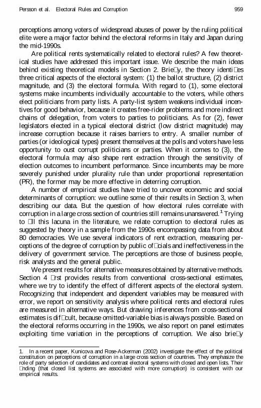
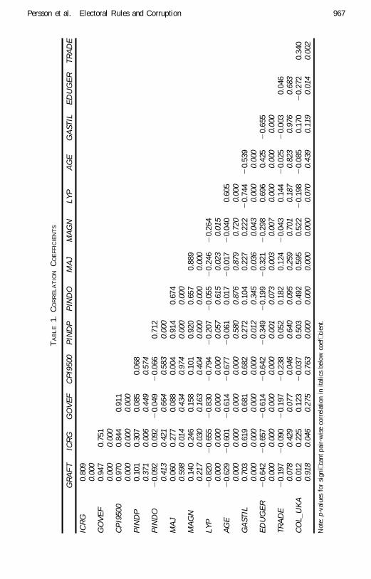
As already mentioned, different aspects of electoral systems are stronglycorrelated across countries. Table 1 lists the simple correlation coef� cientsamong the main variables in our cross-sectional data set. The correlationcoef� cients among the two continuous measures PINDP, MAGN and the binarymeasure MAJ are all around 0.9, whereas the correlation between these threemeasures and PINDO is between 0.6 and 0.7. But while PINDP, PINDO, andMAGN are continuous measures of different features of electoral rules, thevariable MAJ is a binary measure lumping together proportional and mixedelectoral rules into one group, and those countries relying on plurality for thewhole lower house in the other.

3.2 Corruption and Political Rents

It is not easy to � nd an empirical counterpart to rent extraction by politicians.Real-world abuse of higher political of� ce can show up both in outrightcorruption and, more generally, in misgovernance. We use four different mea-


TA

BL

E1.

CO

RR

EL

AT

ION

CO

EFF

ICIE

NT

S

GR

AF

TIC

RG

GO

VE

FC

PI9

500

PIN

DP

PIN

DO

MA

JM

AG

NLY

PA

GE

GA

STIL

ED

UG

ER

TR

AD

E

ICR

G0.

809

0.00

0G

OV

EF

0.94

70.

751

0.00

00.

000

CP

I950

00.

970

0.84

40.

911

0.00

00.

000

0.00

0P

IND

P0.

101

0.30

70.

085

0.06

80.

371

0.00

60.

449

0.57

4P

IND

O2

0.09

20.

092

20.

049

20.

066

0.71

20.

413

0.42

10.

664

0.58

30.

000

MA

J0.

060

0.27

70.

088

0.00

40.

914

0.67

40.

598

0.01

40.

434

0.97

40.

000

0.00

0M

AG

N0.

140

0.24

60.

158

0.10

10.

920

0.65

70.

889

0.21

70.

030

0.16

30.

404

0.00

00.

000

0.00

0LY

P2

0.82

02

0.65

52

0.83

02

0.79

42

0.20

72

0.05

52

0.24

62

0.26

40.

000

0.00

00.

000

0.00

00.

057

0.61

50.

023

0.01

5A

GE

20.

629

20.

601

20.

614

20.

677

20.

061

0.01

72

0.01

72

0.04

00.

605

0.00

00.

000

0.00

00.

000

0.58

00.

876

0.87

90.

720

0.00

0G

AST

IL0.

703

0.61

90.

681

0.68

20.

272

0.10

40.

227

0.22

22

0.74

42

0.53

90.

000

0.00

00.

000

0.00

00.

012

0.34

50.

036

0.04

30.

000

0.00

0E

DU

GE

R2

0.64

22

0.65

72

0.61

42

0.64

22

0.34

92

0.19

92

0.32

12

0.29

80.

696

0.42

52

0.65

50.

000

0.00

00.

000

0.00

00.

001

0.07

30.

003

0.00

70.

000

0.00

00.

000

TRA

DE

20.

197

20.

090

20.

197

20.

238

0.05

20.

182

0.12

42

0.04

30.

144

20.

025

20.

003

0.04

60.

078

0.42

90.

077

0.04

60.

640

0.09

50.

259

0.70

10.

187

0.82

30.

976

0.68

3C

OL_

UK

A0.

012

0.22

50.

123

20.

037

0.50

30.

492

0.59

50.

522

20.

198

20.

085

0.17

02

0.27

20.

340

0.91

80.

046

0.27

50.

763

0.00

00.

000

0.00

00.

000

0.07

00.

439

0.11

90.

014

0.00

2

Not

e:p -

valu

esfo

rsi

gni�

cant

pair

-wis

eco

rrel

atio

nin

itali

csbe

low

coef

�cie

nt.


sures of political rents; three of these refer to corruption, the fourth to (in)ef-fectiveness in the provision of government services.

As Tanzi (1998) observes, it is dif� cult to de� ne corruption in the abstract.Moreover, as corruption is generally illegal, violators try to keep it secret.Cultural and legal differences across countries make it hard to investigatecorruption without taking country-speci� c features into account. Good proxiesfor political corruption should thus offer reliable information on the unlawfulabuse of political power, as well as a strong level of comparability acrossdifferent countries.

The Corruption Perceptions Index goes some way towards meeting theserequirements.8 It is produced by Transparency International, an NGO heavilyinvolved in raising the public awareness about corruption and ways of combat-ting it. This index measures the “perceptions of the degree of corruption as seenby business people, risk analysts and the general public” and is computed as thesimple average of a number of different surveys assessing each country’sperformance in a given year. For example, the 1998 score is based on 12 surveysfrom 7 different institutions. Each score ranges between 0 (perfectly clean) and10 (highly corrupt). As discussed at length in Lambsdorff (1998), the results ofthese surveys are highly positively correlated: the pair-wise correlation coef� -cient among different surveys exceeds 0.8 on average, suggesting that theindependent surveys really measure some common features. Dispersion in theranking for an individual country is an indicator of measurement error in theaverage score. For this reason, we typically weigh observations with the (inverseof the) standard deviation among the different surveys available for eachcountry.

We use this variable only in the cross-sectional analysis, taking the averageof yearly country scores, available from 1995 to 2000. This variable, calledCPI9500, is one of our measures of corruption. It is available for 72 countries,with a mean of 4.8 and a standard deviation of 2.4. The lowest recorded valueis 0.3 (for Denmark) and the highest 8.3 (for Honduras and Paraguay).

An alternative corruption measure is based on a similar survey of surveyspresented and discussed in Kaufman, Kraay, and Zoido-Lobaton (1999). Here,the original surveys refer to the years 1997 and 1998. The observed surveyresults are combined into different clusters of governance indicators by astatistical, unobserved-components procedure. We use their sixth cluster called“Graft.” According to the authors, this particular cluster captures the success ofa society in developing an environment where fair and predictable rules form thebasis for economic and social interactions; perceptions of corruption also playa central role. The original surveys range from 22.5 to 2.5, with higher valuescorresponding to less corruption. We invert and re-scale this measure to thesame 0 –10 scale as CPI9500, while keeping the same name, GRAFT, as in the

8. A number of recent empirical studies of corruption have employed this index, includingFisman and Gatti (1999), Treisman (2000) and Wei (1997a and 1997b).


original source. In this case as well, we weight the observations with thestandard deviation of the original surveys.

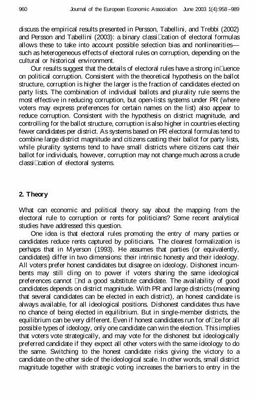
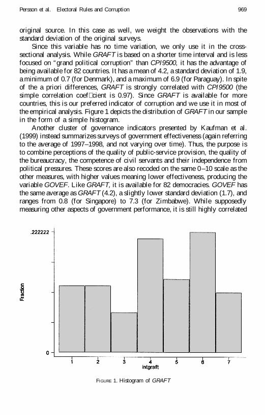
Since this variable has no time variation, we only use it in the cross-sectional analysis. While GRAFT is based on a shorter time interval and is lessfocused on “grand political corruption” than CPI9500, it has the advantage ofbeing available for 82 countries. It has a mean of 4.2, a standard deviation of 1.9,a minimum of 0.7 (for Denmark), and a maximum of 6.9 (for Paraguay). In spiteof the a priori differences, GRAFT is strongly correlated with CPI9500 (thesimple correlation coef� cient is 0.97). Since GRAFT is available for morecountries, this is our preferred indicator of corruption and we use it in most ofthe empirical analysis. Figure 1 depicts the distribution of GRAFT in our samplein the form of a simple histogram.

Another cluster of governance indicators presented by Kaufman et al.(1999) instead summarizes surveys of government effectiveness (again referringto the average of 1997–1998, and not varying over time). Thus, the purpose isto combine perceptions of the quality of public-service provision, the quality ofthe bureaucracy, the competence of civil servants and their independence frompolitical pressures. These scores are also recoded on the same 0–10 scale as theother measures, with higher values meaning lower effectiveness, producing thevariable GOVEF. Like GRAFT, it is available for 82 democracies. GOVEF hasthe same average as GRAFT (4.2), a slightly lower standard deviation (1.7), andranges from 0.8 (for Singapore) to 7.3 (for Zimbabwe). While supposedlymeasuring other aspects of government performance, it is still highly correlated

FIGURE 1. Histogram of GRAFT


with the corruption measures (the correlation is 0.91 with CPI9500 and 0.95with GRAFT).

Finally, the International Country Risk Guide (ICRG) corruption index isthe only one spanning the whole 1990 –1998 period, and we mainly use it in thepanel analysis, to explore the effects of electoral reforms. Like the othermeasures, we re-scaled it to vary between 0 and 10, with higher values denotingmore corruption. This index has been used in some earlier studies, includingAdes and Di Tella (1999). It is released by Political Risk Services, a privatethink tank specialized in international political and economic country-riskassessments. The index is based on the opinion of a pool of country analysts andrefers to the following issues: “high government of� cials are likely to demandspecial payments”; “illegal payments are generally expected throughout lowerlevels of government” in the form of “bribes connected with import and exportlicences, exchange controls, tax assessments, police protection, or loans.”

3.3 Other Explanatory Variables

Earlier empirical work based on cross-country data has identi� ed a number ofeconomic, social, cultural, historical and geographical variables that correlatewith the incidence of corruption. We follow these earlier studies in formulatinga basic empirical speci� cation.

To take account of economic development, we consider the logarithm ofGNP per capita, adjusted for purchasing power (LYP), and a dummy variable forOECD membership (OECD). We expect both these variables to be associatedwith less corruption. Because earlier work has shown openness to trade to benegatively correlated with corruption (see Ades and Di Tella 1999), we alsocontrol for a measure of openness (TRADE), de� ned as the sum of exports andimports as a percentage of GDP).

Based on the existing literature, we also try some other country character-istics. Several recent studies have found a higher fractionalization of thepopulation in the linguistic or ethnic dimension to be a signi� cant determinantof misgovernance (see e.g., Mauro 1995 and La Porta, Lopez-De Silanes,Shleifer, and Vishny 1999). We use one widely available measure of linguisticand ethnic fractionalization, which itself is put together as an average of � vedifferent indexes (AVELF). This measure goes from 0 to 1, with higher valuescorresponding to more fractionalization. It is also likely that a more educatedpopulation will suffer less from rent extraction by politicians. To allow for thispossibility, we measure the country’s level of education by the secondary schoolgross enrolment ratio (for male and female population) (EDUGER). Severalauthors have also found religious beliefs to be signi� cantly associated with moreor less corruption (see e.g., Treisman 2000). To allow for this possibility, we usea continuous measure of the population shares with a Protestant religious


tradition as measured in the 1980s (PROT80) and an indicator variable forConfucian dominance (CONFU).

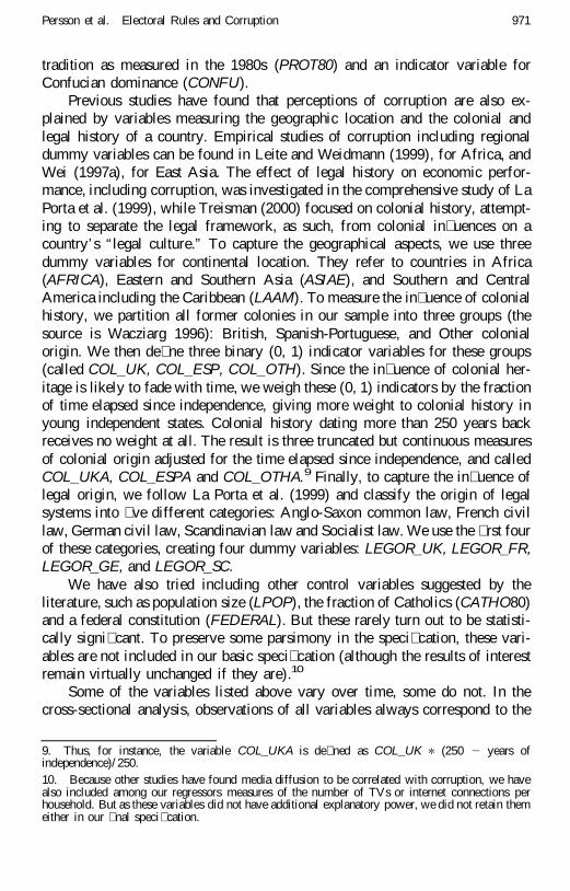
Previous studies have found that perceptions of corruption are also ex-plained by variables measuring the geographic location and the colonial andlegal history of a country. Empirical studies of corruption including regionaldummy variables can be found in Leite and Weidmann (1999), for Africa, andWei (1997a), for East Asia. The effect of legal history on economic perfor-mance, including corruption, was investigated in the comprehensive study of LaPorta et al. (1999), while Treisman (2000) focused on colonial history, attempt-ing to separate the legal framework, as such, from colonial in� uences on acountry’s “legal culture.” To capture the geographical aspects, we use threedummy variables for continental location. They refer to countries in Africa(AFRICA), Eastern and Southern Asia (ASIAE), and Southern and CentralAmerica including the Caribbean (LAAM). To measure the in� uence of colonialhistory, we partition all former colonies in our sample into three groups (thesource is Wacziarg 1996): British, Spanish-Portuguese, and Other colonialorigin. We then de� ne three binary (0, 1) indicator variables for these groups(called COL_UK, COL_ESP, COL_OTH). Since the in� uence of colonial her-itage is likely to fade with time, we weigh these (0, 1) indicators by the fractionof time elapsed since independence, giving more weight to colonial history inyoung independent states. Colonial history dating more than 250 years backreceives no weight at all. The result is three truncated but continuous measuresof colonial origin adjusted for the time elapsed since independence, and calledCOL_UKA, COL_ESPA and COL_OTHA.9 Finally, to capture the in� uence oflegal origin, we follow La Porta et al. (1999) and classify the origin of legalsystems into � ve different categories: Anglo-Saxon common law, French civillaw, German civil law, Scandinavian law and Socialist law. We use the � rst fourof these categories, creating four dummy variables: LEGOR_UK, LEGOR_FR,LEGOR_GE, and LEGOR_SC.

We have also tried including other control variables suggested by theliterature, such as population size (LPOP), the fraction of Catholics (CATHO80)and a federal constitution (FEDERAL). But these rarely turn out to be statisti-cally signi� cant. To preserve some parsimony in the speci� cation, these vari-ables are not included in our basic speci� cation (although the results of interestremain virtually unchanged if they are).10

Some of the variables listed above vary over time, some do not. In thecross-sectional analysis, observations of all variables always correspond to the

9. Thus, for instance, the variable COL_UKA is de� ned as COL_UK p (250 2 years ofindependence)/ 250.10. Because other studies have found media diffusion to be correlated with corruption, we havealso included among our regressors measures of the number of TVs or internet connections perhousehold. But as these variables did not have additional explanatory power, we did not retain themeither in our � nal speci� cation.


country average over the period 1990 –1998. Naturally, in the panel analysis weonly include annual observations of the time-varying variables.

3.4 Preliminary Analysis

In this subsection, we report some preliminary statistical analysis for thecross-sectional data. To save space, and given the high correlation among allmeasures of corruption, in this subsection we focus exclusively on the variableGRAFT which is available for more countries. Results for the other indicators ofpolitical rents and corruption are very similar.

Table 1 shows the correlation coef� cients among some of the main vari-ables. A number of these are highly correlated, as expected. Richer economieshave more educated populations and are better and older democracies. Judgingfrom the simple correlations, corruption is lower in richer economies, in betterand older democracies, and countries where the population is better educated.

As mentioned earlier, the electoral variables of most interest, PINDP(alternatively PINDO), MAJ, and MAGN, are highly positively correlated witheach other. Multicollinearity may thus be a problem, particularly if the variablesare predicted to affect corruption in the same direction (as PINDP and MAJ). Onthe other hand, these variables are not very strongly correlated with otherindependent variables (with the exception of COL_UKA), which suggests thatmulticollinearity with the other controls is unlikely to be a major problem. Notethat the electoral variables display little direct correlation with corruption.

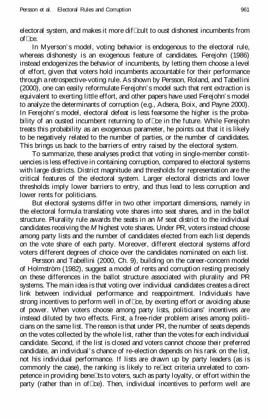
Before turning to a systematic analysis of electoral rules, we ask how wellthe observed cross-country variation in corruption can be explained by othersocial, economic and institutional variables. A concise summary of the answeris given in Figure 2. Here, we display the distribution of the residuals in GRAFTfrom a regression encompassing the standard determinants of corruption dis-cussed in the previous subsection, including colonial history (the speci� cationomits the measures of the electoral rule and the dummy variable for geographiclocation and legal history). Altogether, the basic economic, social and historicalvariables explain over 85 percent of the variation in the data. The residuals rangefrom 21.86, for Chile, to 12.11, for Papua New Guinea (the way we measureGRAFT, a negative residual means less corruption than predicted). Other coun-tries with residuals close to 1.5 or more in absolute value include Cyprus andSenegal (both negative), Belgium, Bahamas, Venezuela, and Jamaica (all pos-itive). Clearly, our basic controls eliminate the most striking differences acrosscountries.

The precise speci� cation and estimated coef� cients of the regression gen-erating these residuals are displayed at the bottom of Figure 2.11 Corruption is

11. Estimation is by weighted least squares, the weights being the (inverse) standard deviation ofGRAFT.


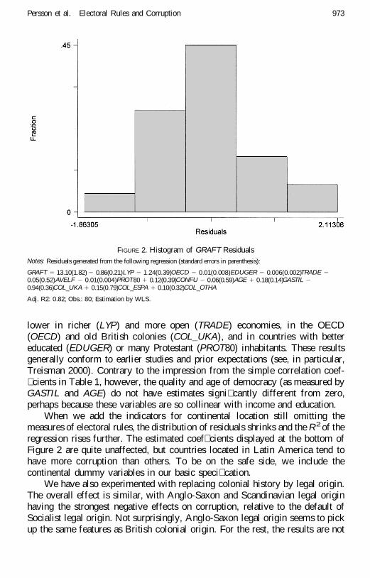
lower in richer (LYP) and more open (TRADE) economies, in the OECD(OECD) and old British colonies (COL_UKA), and in countries with bettereducated (EDUGER) or many Protestant (PROT80) inhabitants. These resultsgenerally conform to earlier studies and prior expectations (see, in particular,Treisman 2000). Contrary to the impression from the simple correlation coef-� cients in Table 1, however, the quality and age of democracy (as measured byGASTIL and AGE) do not have estimates signi� cantly different from zero,perhaps because these variables are so collinear with income and education.

When we add the indicators for continental location still omitting themeasures of electoral rules, the distribution of residuals shrinks and the R2 of theregression rises further. The estimated coef� cients displayed at the bottom ofFigure 2 are quite unaffected, but countries located in Latin America tend tohave more corruption than others. To be on the safe side, we include thecontinental dummy variables in our basic speci� cation.

We have also experimented with replacing colonial history by legal origin.The overall effect is similar, with Anglo-Saxon and Scandinavian legal originhaving the strongest negative effects on corruption, relative to the default ofSocialist legal origin. Not surprisingly, Anglo-Saxon legal origin seems to pickup the same features as British colonial origin. For the rest, the results are not

FIGURE 2. Histogram of GRAFT ResidualsNotes: Residuals generated from the following regression (standard errors in parenthesis):

GRAFT 5 13.10(1.82) 2 0.86(0.21)LYP 2 1.24(0.39)OECD 2 0.01(0.008)EDUGER 2 0.006(0.002)TRADE 20.05(0.52)AVELF 2 0.01(0.004)PROT80 1 0.12(0.39)CONFU 2 0.06(0.59)AGE 1 0.18(0.14)GASTIL 20.94(0.36)COL_UKA 1 0.15(0.79)COL_ESPA 1 0.10(0.32)COL_OTHA

Adj. R2: 0.82; Obs.: 80; Estimation by WLS.


affected much. Since the speci� cation with the colonial origin indicators are theleast favorable to the results on electoral rules, we always use colonial ratherthan legal origin.

4. Results

4.1 Speci� cation

As discussed in Section 2, the predictions we want to take to the data are notmutually exclusive, each prediction emphasizing a different aspect of electoralrules. This suggests that we ought to estimate a comprehensive speci� cation,where we include all three measures discussed in Section 3, namely theindicators for district magnitude (MAGN), ballot structure (either PINDP orPINDO), and the electoral formula (MAJ). Given that PINDP, PINDO, andMAGN vary continuously, while MAJ is a binary measure of features of theelectoral formula correlated with district magnitude and ballot structure, thiscomprehensive speci� cation can also be considered as a test for nonlineareffects (i.e., does a change in the electoral rule for the whole legislature haveadditional effects on corruption, besides those captured by the continuousindicators). Our � rst benchmark speci� cation thus includes all three measures ofthe electoral rule.

As already noted, however, these three indicators do not have much inde-pendent variation. In particular, it is dif� cult to disentangle the effect of theelectoral formula and that of the ballot structure when the latter is measured byPINDP, since the correlation coef� cient between PINDP and MAJ is 0.91, andthese two variables have the same expected effect on corruption. For this reason,we systematically try a more parsimonious speci� cation, where we alwaysinclude the measure of district magnitude (MAGN), but drop one of the othertwo indicators, either for the electoral formula or the ballot structure. While theestimated coef� cient of district magnitude (MAGN) unambiguously captures thebarriers-to-entry effect (hypothesis H1), the estimated coef� cient of the otherincluded variable could capture the effect of either the career-concern effect(H2) or the electoral formula (H3), irrespective of how it is measured. We alsosystematically experiment with our two different measures for the ballot struc-ture, PINDP and PINDO. Naturally, the interpretation of the results changeswith the speci� cation.

For the rest, the cross-sectional speci� cation always includes the economic,social and historical variables described in Section 3 and listed at the bottom ofFigure 2. Generally, we also control for continental location to minimize the riskof omitted-variable bias. To help reduce the noise introduced by measurementerror, the estimation method is weighted least squares, with weights given by the(inverse) standard deviation of the perceptions of corruption. The results when


we estimate with OLS are similar, although the (robust) standard errors of theestimates are slightly higher. If the standard deviation of the perceptions ofcorruption is not available, as when corruption is measured by ICRG, weestimate by OLS and report robust standard errors.

4.2 Basic OLS estimates

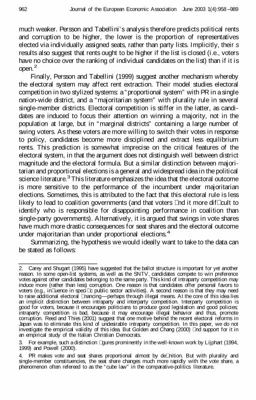
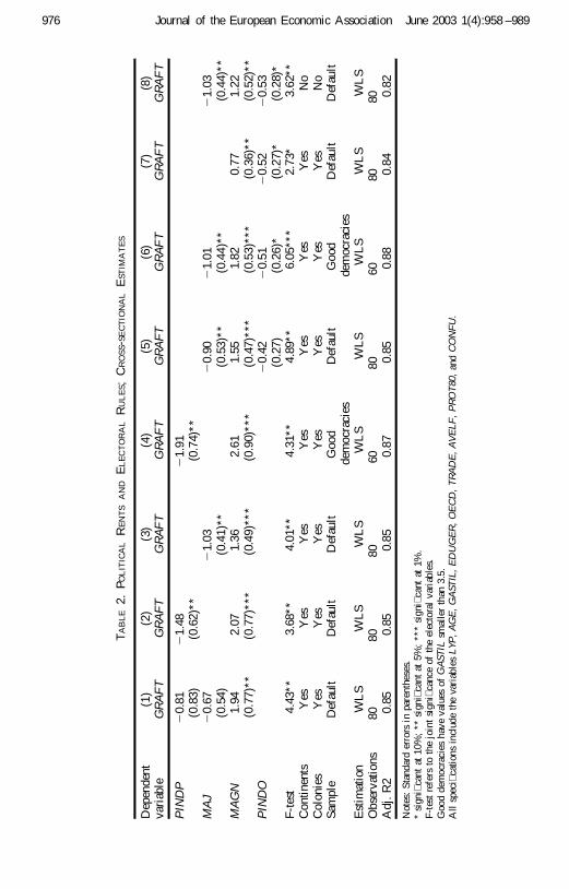
Our � rst regression results are reported in Table 2. As we have the largestnumber of observations for GRAFT, we start with this corruption measure as ourdependent variable. In the � rst four columns, we measure the ballot structurewith the strict measure of voting over individuals, PINDP. Column 1 reports onthe most comprehensive speci� cation, where we include all three indicators forthe electoral rule. All three estimated coef� cients have the expected sign, i.e.,negative for PINDP and MAJ and positive for MAGN. While the coef� cient ondistrict magnitude is clearly signi� cantly different from zero (p-value of 0.015),the coef� cients on the ballot structure and the electoral formula are not (p-valuesof 0.22 and 0.33, respectively). As noted previously, the latter might be due tothe high correlation between the variables PINDP and MAJ. As shown inColumns 2 and 3, when we drop either of these variables, the remaining onebecomes signi� cantly different from zero, while district magnitude also remainsstrongly signi� cant. Column 4 shows that the coef� cients become larger inabsolute value and more precisely estimated when the sample is cut by 25percent, restricting it to better democracies (i.e., those with an average GASTILscore smaller than 3.5).

Notice that the estimated coef� cients of PINDP (alternatively MAJ) andMAGN are large (all variables are de� ned so that they lie between 0 and 1) andtheir standardized beta coef� cients are the largest of all regressors. For example,switching from a system where all legislators are elected by PR on party lists(PINDP 5 0), to one where all are elected by plurality as individuals (PINDP 51) is estimated to reduce the perceptions of corruption by about 20 percent (2points out of 10) in the sample of good democracies. This is about twice theeffect of not being a Latin-American country. The estimated effect of inversedistrict magnitude (also taking positive values below 1) is even larger, thoughit is a bit less stable to the speci� cation. Due to the strong correlation betweenPINDP and MAJ, it is hard to give an unambiguous interpretation of theseestimates, however. They are consistent with a negative career-concern effect,as well as a negative electoral-competition effect (or with both effects beingoperative at the same time).

While the variable PINDP captures the free-rider problem associated withlist voting under PR, it does not discriminate between open and closed lists. Tocapture this second effect of electoral rules suggested by the career-concernmodel, we replace PINDP by the other measure of ballot-structure, PINDO. Asdiscussed in Section 3, this means that we now also treat as individually elected


TA

BL

E2.

POL

ITIC

AL

RE

NT

SA

ND

EL

EC

TO

RA

LR

UL

ES;

CR

OSS

-SE

CT

ION

AL

EST

IMA

TE

S

Dep

ende

ntva

riab

le(1

)G

RA

FT

(2)

GR

AF

T(3

)G

RA

FT

(4)

GR

AF

T(5

)G

RA

FT

(6)

GR

AF

T(7

)G

RA

FT

(8)

GR

AF

T

PIN

DP

20.

812

1.48

21.

91(0

.83)

(0.6

2)**

(0.7

4)**

MA

J2

0.67

21.

032

0.90

21.

012

1.03

(0.5

4)(0

.41)

**(0

.53)

**(0

.44)

**(0

.44)

**M

AG

N1.

942.

071.

362.

611.

551.

820.

771.

22(0

.77)

**(0

.77)

***

(0.4

9)**

*(0

.90)

***

(0.4

7)**

*(0

.53)

***

(0.3

6)**

(0.5

2)**

PIN

DO

20.

422

0.51

20.

522

0.53

(0.2

7)(0

.26)

*(0

.27)

*(0

.28)

*F

-tes

t4.

43**

3.68

**4.

01**

4.31

**4.

89**

6.05

***

2.73

*3.

62**

Con

tinen

tsY

esY

esY

esY

esY

esY

esY

esN

oC

olon

ies

Yes

Yes

Yes

Yes

Yes

Yes

Yes

No

Sam

ple

Def

ault

Def

ault

Def

ault

Goo

dde

moc

raci

esD

efau

ltG

ood

dem

ocra

cies

Def

ault

Def

ault

Est

imat

ion

WL

SW

LS

WL

SW

LS

WL

SW

LS

WL

SW

LS

Obs

erva

tion

s80

8080

6080

6080

80A

dj.

R2

0.85

0.85

0.85

0.87

0.85

0.88

0.84

0.82

Not

es:

Sta

ndar

der

rors

inpa

rent

hese

s.*

sign

i�ca

ntat

10%

;**

sign

i�ca

ntat

5%;

***

sign

i�ca

ntat

1%.

F-t

est

refe

rsto

the

join

tsi

gni�

canc

eof

the

elec

tora

lva

riab

les.

Goo

dde

moc

raci

esha

veva

lues

ofG

AST

ILsm

alle

rth

an3.

5.A

llsp

eci�

catio

nsin

clud

eth

eva

riab

les

LYP

,A

GE

,G

AST

IL,

ED

UG

ER

,O

EC

D,

TR

AD

E,

AV

ELF

,P

RO

T80

,an

dC

ON

FU

.


those politicians obtaining their seats via (semiproportional) STV systems andvia open lists in PR party-list systems. Recall that PINDO indeed has a lowercorrelation (0.67) with our measure of the electoral formula (MAJ) than PINDP.Column 5 reports on the same comprehensive speci� cation as Column 1.Inverse district magnitude continues to have a signi� cant positive effect oncorruption. The coef� cient on the indicator for plurality rule (MAJ) goes up bya third (in absolute value) and now becomes signi� cantly different from zero.On the other hand, the coef� cient on individual ballots (PINDO) falls somewhat(in absolute value) but also becomes more precisely estimated ( p-value of 0.12).When the sample is restricted to good democracies in Column 6, the pointestimates remain about the same, but now all three coef� cients are signi� cantlydifferent from zero. When we omit MAJ from the regression, as in Column 7,the coef� cient on the ballot structure stays roughly the same. But the coef� cienton district magnitude drops by more than half its previous value: as districtmagnitude is strongly correlated with the electoral formula, this coef� cient isforced to pick up the negative effect of the omitted variable.

Finally, Column 8 shows the effect of dropping the indicators of continentsand colonial history from the speci� cation in Column 5. The effect of all threeelectoral indicators now becomes statistically signi� cant. If we instead replacecolonial history by our measures of legal history in the speci� cation of Column5, this also raises the precision of the estimates such that all three electoralvariables are once more signi� cantly different from zero (results nor shown).These results are reassuring, because a history as a former British colony or aBritish-style legal system, in particular, not only appears to reduce the currentpropensity for corruption. It also tends to exert a strong in� uence on a country’selectoral institutions, making a British style � rst-past-the-post system muchmore likely (MAJ has a correlation of 0.60 with COL_UKA and 0.70 withLEGOR_UK). Thus, the results had better be robust to including these variablesas controls. As a � nal check, the results are also robust to cutting the mostin� uential observations, following the approach recommended by Belsley, Kuh,and Welsh (1980).12

Judging from these estimates, the free-rider problem captured by the indi-cator PINDP seems to have a stronger and more robust effect on corruption,compared the closed-list system captured by PINDO. If the ballot structureindeed shapes corruption, the effect seems to go through the incentive problemsassociated with free riding, while the distinction between open and closed lists

12. There is one important fragility in the estimates reported in Table 2, however. It concernsChile, a country with low corruption (and a highly negative estimated residual) and a peculiarelectoral system. As noted in Footnote 6, Chile’s electoral system is hard to classify. Unfortunately,this single observation and our classi� cation matter for our results. Dropping Chile from thesample, or reclassifying its electoral system so that MAJ 5 0 (rather than 1) and PINDP 5 0 (ratherthan 1), the estimated effects of the electoral variables on corruption become less preciselyestimated and lose signi� cance. Chile is not the only outlier observation, however, and droppingChile together with other in� uential observations does not signi� cantly affect the results reportedin Table 2.


seems less important. As noted before, however, the variable PINDP might alsore� ect the importance of the electoral formula, as emphasized by the electoral-competition effect (hypothesis H3).

4.3 Estimates with Alternative Measurement

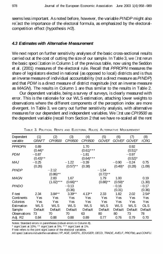
We next report on further sensitivity analyses of the basic cross-sectional resultscarried out at the cost of cutting the size of our sample. In Table 3, we � rst rerunthe basic speci� cation in Column 1 of the previous table, now using the Seddonet al. (2001) measures of the electoral rule. Recall that PPROPN measures theshare of legislators elected in national (as opposed to local) districts and is thusan inverse measure of individual accountability (not a direct measure as PINDP)and that PDM is a direct measure of district magnitude (not an inverse measureas MAGN). The results in Column 1 are thus similar to the results in Table 2.

Our dependent variable, being a survey of surveys, is clearly measured witherror. This is the rationale for our WLS estimation, attaching lower weights toobservations where the different components of the perception index are moredivergent. In Table 3, we carry out further sensitivity analysis, with alternativemeasures for our dependent and independent variables. We � rst use CPI9500 asthe dependent variable (recall from Section 2 that we have re-scaled all the rent

TABLE 3. POLITICAL RENTS AND ELECTORAL RULES; ALTERNATIVE MEASUREMENT

Dependentvariable

(1)GRAFT

(2)CPI9500

(3)CPI9500

(4)CPI9500

(5)GOVEF

(6)GOVEF

(7)GOVEF

(8)ICRG

PPROPN 0.89 1.70 0.92(0.44)* (0.61)*** (0.51)*

PDM 20.87 21.81 20.97(0.43)** (0.64)*** (0.52)*

MAJ 20.25 21.22 20.39 20.90 20.24 0.75(0.26) (0.57)** (0.38) (0.49)* (0.28) (1.09)

PINDP 22.12 21.54(0.86)** (0.72)**

MAGN 2.83 1.67 1.79 1.00 0.19(1.02)*** (0.66)** (0.88)** (0.59)* (1.30)

PINDO 20.13 20.16 20.17(0.36) (0.31) (0.36)

F-test 2.34 3.84** 3.39** 4.13** 2.33 1.82 2.02 2.54*Continents Yes Yes Yes Yes Yes Yes Yes YesColonies Yes Yes Yes Yes Yes Yes Yes YesEstimation WLS WLS WLS WLS WLS WLS WLS OLSSample Default Default Default Default Default Default Default DefaultObservations 73 70 70 63 80 80 73 78Adj. R2 0.84 0.88 0.88 0.89 0.77 0.76 0.79 0.70

Notes: Standard errors in parentheses (robust errors in Column 8).* signi� cant at 10%; ** signi� cant at 5%; *** signi� cant at 1%.F-test refers to the joint signi� cance of the electoral variables.All speci� cations include the variables LYP, AGE, GASTIL, EDUGER, OECD, TRADE, AVELF, PROT80, and CONFU.


extraction measures to run between 0 and 10). Columns 2 and 3 correspond tocolumns 2 and 5 in Table 2, while Column 4 corresponds to Column 1 in Table3. Basically, the results are the same as before. The results in the speci� cationswith PINDP and the Seddon et al. variables indicate slightly stronger effects ofthe electoral system than the results for GRAFT. The results in the speci� cationwith PINDO indicate even more strongly than in Table 2 that it is the lack of afree-rider problem under plurality rule rather than open vs. closed lists that hasbite on corruption. Alternatively, they indicate that the electoral-competitioneffect is stronger than the career-concern effect.

Columns 5–7 show the results of the same speci� cations when we insteaduse GOVEF, the measure of ineffectiveness in the provision of public services,as the dependent variable. The general pattern of results is the same as forCPI9500, even though the coef� cients of interest are less precisely estimatedand the general � t of the regression is poorer.

Finally, Column 8 shows an example of the results when we use the averageof our time-varying corruption measure ICRG as the dependent variable. Here,the results are more disappointing, given our theoretical hypotheses. None of themeasures of interest has a statistically signi� cant coef� cient (even though thethree variables together are marginally signi� cant). Individual accountabilityappears to be important when measured by PPROPN (result not shown). As forGOVEF, the � t of the regression is considerably poorer than previously, indi-cating that ICRG is a noisy measure of corruption. Unfortunately, as the ICRGmeasure is derived from a single source, we cannot use the WLS approach toadjust our estimates for measurement error in this case.

4.4 Panel Estimates

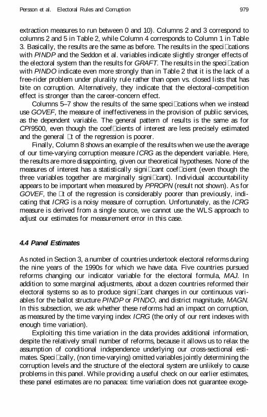
As noted in Section 3, a number of countries undertook electoral reforms duringthe nine years of the 1990s for which we have data. Five countries pursuedreforms changing our indicator variable for the electoral formula, MAJ. Inaddition to some marginal adjustments, about a dozen countries reformed theirelectoral systems so as to produce signi� cant changes in our continuous vari-ables for the ballot structure PINDP or PINDO, and district magnitude, MAGN.In this subsection, we ask whether these reforms had an impact on corruption,as measured by the time varying index ICRG (the only of our rent indexes withenough time variation).

Exploiting this time variation in the data provides additional information,despite the relatively small number of reforms, because it allows us to relax theassumption of conditional independence underlying our cross-sectional esti-mates. Speci� cally, (non time-varying) omitted variables jointly determining thecorruption levels and the structure of the electoral system are unlikely to causeproblems in this panel. While providing a useful check on our earlier estimates,these panel estimates are no panacea: time variation does not guarantee exoge-


neity. Obviously, we must still assume that the political events leading to theobserved electoral reforms were not accompanied by signi� cant changes inunobserved determinants of corruption.

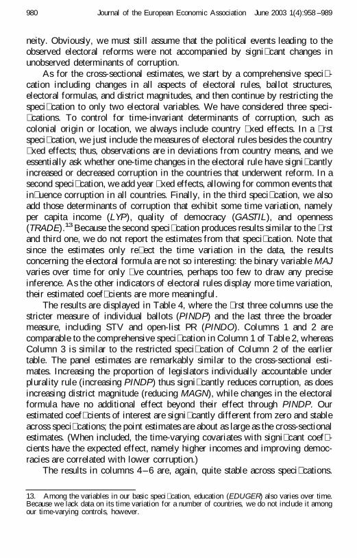
As for the cross-sectional estimates, we start by a comprehensive speci� -cation including changes in all aspects of electoral rules, ballot structures,electoral formulas, and district magnitudes, and then continue by restricting thespeci� cation to only two electoral variables. We have considered three speci-� cations. To control for time-invariant determinants of corruption, such ascolonial origin or location, we always include country � xed effects. In a � rstspeci� cation, we just include the measures of electoral rules besides the country� xed effects; thus, observations are in deviations from country means, and weessentially ask whether one-time changes in the electoral rule have signi� cantlyincreased or decreased corruption in the countries that underwent reform. In asecond speci� cation, we add year � xed effects, allowing for common events thatin� uence corruption in all countries. Finally, in the third speci� cation, we alsoadd those determinants of corruption that exhibit some time variation, namelyper capita income (LYP), quality of democracy (GASTIL), and openness(TRADE).13 Because the second speci� cation produces results similar to the � rstand third one, we do not report the estimates from that speci� cation. Note thatsince the estimates only re� ect the time variation in the data, the resultsconcerning the electoral formula are not so interesting: the binary variable MAJvaries over time for only � ve countries, perhaps too few to draw any preciseinference. As the other indicators of electoral rules display more time variation,their estimated coef� cients are more meaningful.

The results are displayed in Table 4, where the � rst three columns use thestricter measure of individual ballots (PINDP) and the last three the broadermeasure, including STV and open-list PR (PINDO). Columns 1 and 2 arecomparable to the comprehensive speci� cation in Column 1 of Table 2, whereasColumn 3 is similar to the restricted speci� cation of Column 2 of the earliertable. The panel estimates are remarkably similar to the cross-sectional esti-mates. Increasing the proportion of legislators individually accountable underplurality rule (increasing PINDP) thus signi� cantly reduces corruption, as doesincreasing district magnitude (reducing MAGN), while changes in the electoralformula have no additional effect beyond their effect through PINDP. Ourestimated coef� cients of interest are signi� cantly different from zero and stableacross speci� cations; the point estimates are about as large as the cross-sectionalestimates. (When included, the time-varying covariates with signi� cant coef� -cients have the expected effect, namely higher incomes and improving democ-racies are correlated with lower corruption.)

The results in columns 4–6 are, again, quite stable across speci� cations.

13. Among the variables in our basic speci� cation, education (EDUGER) also varies over time.Because we lack data on its time variation for a number of countries, we do not include it amongour time-varying controls, however.


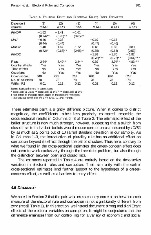
These estimates paint a slightly different picture. When it comes to districtmagnitude, the coef� cients—albeit less precisely estimated—resemble thecross-sectional results in Columns 6 –8 of Table 2. The estimated effect of theballot structure is now much stronger, however, suggesting that a switch fromclosed lists to individual ballots would reduce corruption as measured by ICRGby as much as 2 points out of 10 (a full standard deviation in our sample). Asin Columns 1–3, the introduction of plurality rule has no additional effect oncorruption beyond its effect through the ballot structure. Thus here, contrary towhat we found in the cross-sectional estimates, the career-concern effect doesnot seem to work exclusively through the free-rider problem, but also throughthe distinction between open and closed lists.

The estimates reported in Table 4 are entirely based on the time-seriesvariation in electoral rules and corruption. Their similarity with the earliercross-sectional estimates lend further support to the hypotheses of a career-concerns effect, as well as a barriers-to-entry effect.

4.5 Discussion

We noted in Section 3 that the pair-wise cross-country correlation between eachmeasure of the electoral rule and corruption is not signi� cantly different fromzero (recall Table 1). In this section, we instead document strong and signi� canteffects of the electoral variables on corruption. It might be conjectured that thedifference emanates from our controlling for a variety of economic and social

TABLE 4. POLITICAL RENTS AND ELECTORAL RULES; PANEL ESTIMATES

Dependentvariable

(1)ICRG

(2)ICRG

(3)ICRG

(4)ICRG

(5)ICRG

(6)ICRG

PINDP 21.52 21.41 21.61(0.74)** (0.70)** (0.65)**

MAJ 20.46 20.33 20.19 20.15(0.44) (0.44) (0.47) (0.46)

MAGN 1.40 1.67 1.72 0.46 0.82 0.80(0.72)* (0.68)** (0.68)** (0.55) (0.53) (0.53)

PINDO 21.99 21.70 21.82(0.76)*** (0.72)** (0.64)***

F-test 2.64* 3.49** 3.84** 0.39 3.94** 4.83***Country effects Yes Yes Yes Yes Yes YesTime effects No Yes Yes No Yes YesCovariates No Yes Yes No Yes YesObservations 640 623 623 640 640 623No. of countries 78 78 78 78 78 78Within R2 0.01 0.12 0.12 0.02 0.12 0.12

Notes: Standard errors in parentheses.* signi� cant at 10%; ** signi� cant at 5%; *** signi� cant at 1%.F-test refers to the joint signi� cance of the electoral variables.Time-varying covariates are LYP, GASTIL, and TRADE.


determinants of corruption (in the cross-sectional estimation) or exploiting thetime variation (in the panel estimation). But this conjecture is false, or at bestonly half-true. Consider � rst the cross-country regressions. If we retain the basicspeci� cation of Table 2 (including the dummy variables for continental locationand colonial origin) and add the electoral variables one by one in isolation, noneof them is ever signi� cantly different from zero, in consistency with theinsigni� cant binary correlations. A strong and statistically signi� cant effect ofthe electoral variables is only detected if we condition simultaneously on twofeatures of the electoral system (district magnitude and either the ballot structureindicators or the binary indicator for the electoral formula). Similar results areobtained if we enter the electoral indicators one by one in the panel analysis ofTable 4, although here a drop in statistical signi� cance does not always occur,or is less stark than in the cross-country regressions.

A previous version of the paper (Persson, Tabellini, and Trebbi 2002),studied more in depth the effect on corruption of the electoral formula alone, ascaptured by the variable MAJ.14 Because this is a binary indicator, we canestimate its effect on corruption from cross-country data exploiting now stan-dard techniques in the econometric literature on the treatment effect—see, e.g.,Wooldridge (2002, Ch. 18) for a textbook overview.15 These estimation tech-niques are more general and allow us to relax the assumptions of linearity andconditional independence implicitly underlying the cross-country regressions ofTables 2 and 3. Conditional independence essentially means that the electoralrules are randomly assigned to countries, given the other included regressors.This is clearly a strong assumption. Even though our regressors always includecolonial origin and continental location, it is always possible that we haveomitted some other historical or social variable in� uencing both corruption andthe electoral rule. To relax this assumption in our previous work, we estimatedthe effect of MAJ on corruption by instrumental variables as well as theHeckman estimation procedure allowing for nonrandom treatment.16 To relaxthe linearity assumption, we rely on nonparametric matching methods, based onthe propensity score. These more general estimation methods con� rm thenegative results of the simple regressions: the electoral formula alone does nothave any signi� cant effect on corruption.

While the sensitivity to the set of conditioning variables reduces thegenerality of our inference, it has a plausible explanation. The alternativetheories summarized in Section 2 are complementary, each emphasizing adifferent feature of electoral rule. Moreover, district magnitude is strongly

14. See also Persson and Tabellini (2003).15. Even though the variable MAJ is binary on yearly data, when we take averages over theperiod 1990 –1998, it becomes a fraction for the few countries undertaking reform in that period.In Persson, Tabellini, and Trebbi (2002) we thus code MAJ according to its value before the reform,to preserve it as a binary variable.16. Our instruments are based on the date of origin of the current electoral rule, and exploithistorical waves (or “fashions”) in the design of electoral rules.


negatively correlated with the other electoral indicators in the real world. Thus,if we only include one feature of the electoral rule in our speci� cation, astandard omitted-variable problem biases the estimate of the included variabletowards zero. Indeed, when at least two electoral variables are included, theirestimated coef� cients are jointly statistically signi� cant, as shown by theF-statistics in Tables 2 and 4.

This interpretation of our results also suggests that a comprehensive elec-toral reform, going from a Dutch-style electoral system with closed party listsin a single national constituency to a UK-style system with � rst past the post inone-member districts—i.e., moving PINDP (or PINDO), MAJ, and MAGN from(approximately) 0 to 1—would have counteracting effects on corruption, pro-ducing a net result close to zero.

5. Conclusion

This paper has presented new empirical results on how electoral rules affectpolitical corruption. The main lesson of the data is that corruption is affected byelectoral institutions, but what matters is the comprehensive design of theelectoral rule, not just a single feature.

Our empirical results differ somewhat depending on exactly how we mea-sure the dependent and independent variables of interest, and whether we exploitthe cross-sectional or time-series variation in the data. Overall, however, theresults are broadly consistent with all three theoretical hypotheses, H1–H3,summarized in Section 2, even though discriminating sharply among the threemay be dif� cult because of the collinearity among our electoral indicators.Countries with smaller electoral districts tend to have more corruption, aspredicted by the barriers-to-entry hypothesis. Countries predominantly votingfor individuals tend to have less corruption than those predominantly voting forparty lists, as predicted by the career-concern hypothesis. There is also somesupport for an additional effect of plurality elections. This can be viewed asevidence for the electoral-competition hypothesis, or as stronger individualcareer concerns in plurality systems than in open-lists systems.

The estimated effects of these details of electoral rules are nontrivial. Forinstance, they may suggest a reason why Estonia has so much less corruptionthan neighboring Latvia—a GRAFT value of 3.8 vs. 5.5—a puzzle for someobservers (see e.g., Bennich-Bjorkman 2002). According to the cross-sectionalestimates in Table 2, 30 percent of the difference is due to Estonia’s open-listsystem, while according to the panel estimates in Table 4, the entire differenceis. Another case of stark differences between neighboring countries is Chile andArgentina with GRAFT values of 2.9 vs. 5.5. The cross-sectional estimatesattribute about 30 percent of the difference to Chile’s use of plurality rule intwo-member districts, with the caveat about classi� cation in Footnote 6. If onealternatively treats Chile as an open-list PR system (Argentina has closed lists),


the panel estimates attribute more than half the corruption difference to theelectoral rule.

We believe the results to be relevant for the design of real-world electoralsystems. For instance, our estimates suggest that Belgium—an outlier withmuch higher corruption than predicted—could cut its corruption level towardsthat of France by holding its legislators individually accountable at the elections.Our results also suggest that each feature of Japan’s recent electoral reform—scrapping plurality rule in some districts and diminishing average districtmagnitude—might actually increase corruption. Italy’s electoral reform—aban-doning PR in favor of plurality rule with direct elections of individuals in singlemember districts for 75% of the legislature—should instead have a mixed effecton corruption. While more direct individual accountability with plurality votingis a step in the right direction, the reduction of average district magnitude hasa countervailing effect. Similarly, New Zealand’s reform of its strictly majori-tarian elections, towards a mixed system with less individual accountability buthigher average district magnitude, might have an ambiguous effect on corrup-tion.

Data Appendix

AFRICA: regional dummy variable for African countries, taking the valueof 1 if a country is African, 0 otherwise.

AGE: age of democracy. De� ned as: AGE 5 (2000-DEM_AGE)/200 andvarying between 0 and 1, with US being the oldest democracy (value of 1).Source: see DEM_AGE.

ASIAE: regional dummy variable for East Asian countries, taking the valueof 1 if a country is East Asian, 0 otherwise.

AUTOC: institutionalized autocracy indicator on a scale from 0 to 10.Derived from codings of the competitiveness of political participation, theregulation of participation, the openness and competitiveness of executiverecruitment, and constraints on the chief executive. Source: Polity IV Project^http://www.cidcm.umd.edu/inscr/polity/index.htm&

AVELF: index of ethnolinguistic fractionalization. Approximates the levelof lack of ethnic and linguistic cohesion within a country. Ranges from 0(homogeneous) to 1 (strongly fractionalized) and averages 5 different indexes.Source: La Porta et al. (1999). For Central and Eastern Europe countriescomputations follow Mauro (1995) with data from Quain (1999).

CATHO80: percentage of the population belonging to the Roman Catholicreligion in 1980. Source: La Porta et al. (1999).

CLIST: indicator for closed party lists. Sources: see LIST and SEATS.COL_ESPA: COL_ESPA 5 COL_ES p (250 2 T_INDEP)/250. Combined

effect of COL_ES, describing if a country was a colony of Spain or not, and


T_INDEP, coding years of independence from 0 to 250 (latter value used forcountries that were never colonized). Source: Wacziarg (1996).

COL_OTHA: COL_OTHA 5 COL_OTH p (250 2 T_INDEP)/250. De� nedanalogously to COL_ESPA. Source: Wacziarg (1996).

COL_UKA: COL_UKA 5 COL_UK p (250 2 T_INDEP)/250. De� nedanalogously to COL_ESPA. Source: Wacziarg (1996).

CONFU: religious tradition dummy, equal to 1 if the majority of thepopulation is Confucian/Buddhist/Zen, 0 otherwise. Source: Wacziarg (1996),CIA—The World Factbook 2000.

CPI9500: corruption perception index. Average of the CPI Index over theperiod 1995–2000. Source: Transparency International (www.transparency.de)and Internet Center for Corruption Research ^www.gwdg.de/uwvw&.

DEM_AGE: year of birth of the democracy. Corresponds to the � rst year ofan uninterrupted string of positive yearly POLITY values until the end of thesample, given that the country is also an independent nation (foreign occupationduring WWII not considered an interruption of democracy). Source: see POL-ITY.

DEMOC: institutionalized democracy indicator on a scale from 0 to 10.Derived from codings of the competitiveness of political participation, theregulation of participation, the openness and competitiveness of executiverecruitment, and constraints on the chief executive. Source: Polity IV Project^http://www.cidcm.umd.edu/inscr/polity/index.htm.&

DISTRICTS: number of primary as well as secondary and tertiary (ifapplicable) districts in elections to the lower house. Sources: Quain (1999) andKurian (1998), Cox (1997), and national constitutional documents.

EDUGER: total enrolment in a speci� c level of education, regardless ofage, expressed as a percentage of the of� cial school population correspondingto the same level of education in a given school-year. Computed by dividing thenumber of students at a given level of education regardless of age, by thepopulation of the age-group of� cially corresponding to the given level ofeducation, and multiplying the result by 100. Source: UNESCO—EducationIndicator—Category Participation ^www.unesco.org&.

FEDERAL: federalism dummy. Source: Adsera, Boix and Payne (2000).GASTIL: average of Gastil indexes for civil liberties and political rights.

Measured on a scale from 1 to 7 with 1 representing the highest degree offreedom. Countries whose combined averages for political rights and for civilliberties fall between 1.0 and 2.5 are designated “free,” between 3.0 and 5.5“partly free” and between 5.5 and 7.0 “not free.” Source: Freedom House,Annual Survey of Freedom Country Ratings.

GOVEF: point estimate of “Government Effectiveness,” the third cluster ofKaufmann et al.’s governance indicators. Combines perceptions of the quality ofpublic service provision, the quality of the bureaucracy, the competence of civilservants, the independence of the civil service from political pressures, and thecredibility of the government’s commitment to policies into a single grouping.


Re-scaled to range from 0 to 10 (lower values correspond to better outcomes).Sources: Kaufmann et al. (1999); ^http://www.worldbank.org/wbi/gac&.

GRAFT: point estimate of “Graft,” the sixth cluster of Kaufmann et al.’sgovernance indicators. Captures the success of a society in developing anenvironment where fair and predictable rules form the basis for economic andsocial interactions, focusing particularly on perceptions of corruption. Re-scaledto range from 0 to 10 (lower values correspond to better outcome). Sources:Kaufmann et al. (1999); ^www.worldbank.org/wbi/gac&.

LAAM: regional country dummy, equal to 1 if a country is Latin American(including the Caribbean), 0 otherwise.

LEGOR_(UK, FR, GE, SO, ANDSC): dummy variable for the origin of thelegal system, among � ve possible origins: Anglo-Saxon Common Law (uk),French Civil Law (fr), German Civil Law (ge), Socialist Law (so), and Scan-dinavian Law (sc). Source: La Porta et al. (1999).

LIST: number of lower-house legislators elected through a party list system.Sources: Quain (1999), Kurian (1998), Cox (1997), and national constitutionaldocuments.

LPOP: natural log of the total population. Source: World Bank.LYP: natural log of the per capita real GDP. Sources: Penn World Tables—

mark 5.6 (PW) and The World Bank’s World Development Indicators (WDI)^www.worldbank.org&.

MAGN: inverse of district magnitude, de� ned as DISTRICTS over SEATS.Sources: Quain (1999) and Kurian (1998), Cox (1997), and national constitu-tional documents.

MAJ: indicator for electoral formula, equal to 1 if either majority orplurality rule is the only formula used in the elections of the lower house, 0otherwise. Sources: Cox (1997), International Institute for Democracy andElectoral Assistance (1997), Quain (1999), and Kurian (1998), and nationalconstitutional documents.

OECD: dummy variable for OECD member countries, equal to 1 if acountry is an OECD member, 0 otherwise. Source: Persson and Tabellini(1999).

PDM: alternative indicator of district magnitude, measured as a weightedaverage, where the weight on each district magnitude in a country is the shareof legislators running in districts of that size. Relative to the original variable inSeddon et al. (2001), this variable is divided by 100 so that it takes valuescomparable to those of MAGN.

PINDO: continuous measure of the ballot structure de� ned as 1 2 (LIST/SEATS)CLIST. Source: see LIST and SEATS.

PINDP: continuous measure of the ballot structure, de� ned as 1 2 (LIST/SEATS). Source: see LIST and SEATS.

PPROPN: alternative indicator of ballot structure, measured as the share oflegislators elected in national (secondary or tertiary) districts rather than sub-national (primary) districts. Source: Seddon et al. (2001).


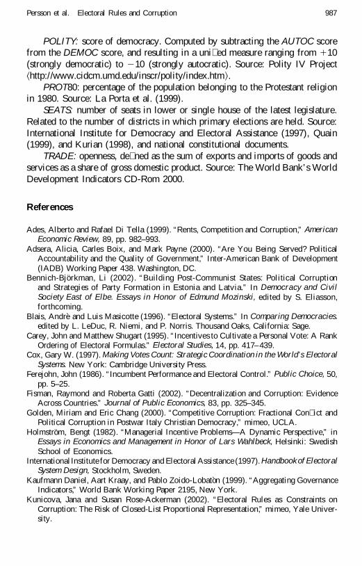
POLITY: score of democracy. Computed by subtracting the AUTOC scorefrom the DEMOC score, and resulting in a uni� ed measure ranging from 110(strongly democratic) to 210 (strongly autocratic). Source: Polity IV Project^http://www.cidcm.umd.edu/inscr/polity/index.htm&.

PROT80: percentage of the population belonging to the Protestant religionin 1980. Source: La Porta et al. (1999).

SEATS: number of seats in lower or single house of the latest legislature.Related to the number of districts in which primary elections are held. Source:International Institute for Democracy and Electoral Assistance (1997), Quain(1999), and Kurian (1998), and national constitutional documents.

TRADE: openness, de� ned as the sum of exports and imports of goods andservices as a share of gross domestic product. Source: The World Bank’s WorldDevelopment Indicators CD-Rom 2000.

References

Ades, Alberto and Rafael Di Tella (1999). “Rents, Competition and Corruption,” AmericanEconomic Review, 89, pp. 982–993.

Adsera, Alicia, Carles Boix, and Mark Payne (2000). “Are You Being Served? PoliticalAccountability and the Quality of Government,” Inter-American Bank of Development(IADB) Working Paper 438. Washington, DC.

Bennich-Bjorkman, Li (2002). “Building Post-Communist States: Political Corruptionand Strategies of Party Formation in Estonia and Latvia.” In Democracy and CivilSociety East of Elbe. Essays in Honor of Edmund Mozinski, edited by S. Eliasson,forthcoming.

Blais, Andre and Luis Masicotte (1996). “Electoral Systems.” In Comparing Democracies.edited by L. LeDuc, R. Niemi, and P. Norris. Thousand Oaks, California: Sage.

Carey, John and Matthew Shugart (1995). “Incentives to Cultivate a Personal Vote: A RankOrdering of Electoral Formulas.” Electoral Studies, 14, pp. 417– 439.

Cox, Gary W. (1997). Making Votes Count: Strategic Coordination in the World’s ElectoralSystems. New York: Cambridge University Press.

Ferejohn, John (1986). “Incumbent Performance and Electoral Control.” Public Choice, 50,pp. 5–25.

Fisman, Raymond and Roberta Gatti (2002). “Decentralization and Corruption: EvidenceAcross Countries.” Journal of Public Economics, 83, pp. 325–345.

Golden, Miriam and Eric Chang (2000). “Competitive Corruption: Fractional Con� ict andPolitical Corruption in Postwar Italy Christian Democracy,” mimeo, UCLA.

Holmstrom, Bengt (1982). “Managerial Incentive Problems—A Dynamic Perspective,” inEssays in Economics and Management in Honor of Lars Wahlbeck, Helsinki: SwedishSchool of Economics.

International Institute for Democracy and Electoral Assistance (1997). Handbook of ElectoralSystem Design, Stockholm, Sweden.

Kaufmann Daniel, Aart Kraay, and Pablo Zoido-Lobaton (1999). “Aggregating GovernanceIndicators,” World Bank Working Paper 2195, New York.

Kunicova, Jana and Susan Rose-Ackerman (2002). “Electoral Rules as Constraints onCorruption: The Risk of Closed-List Proportional Representation,” mimeo, Yale Univer-sity.


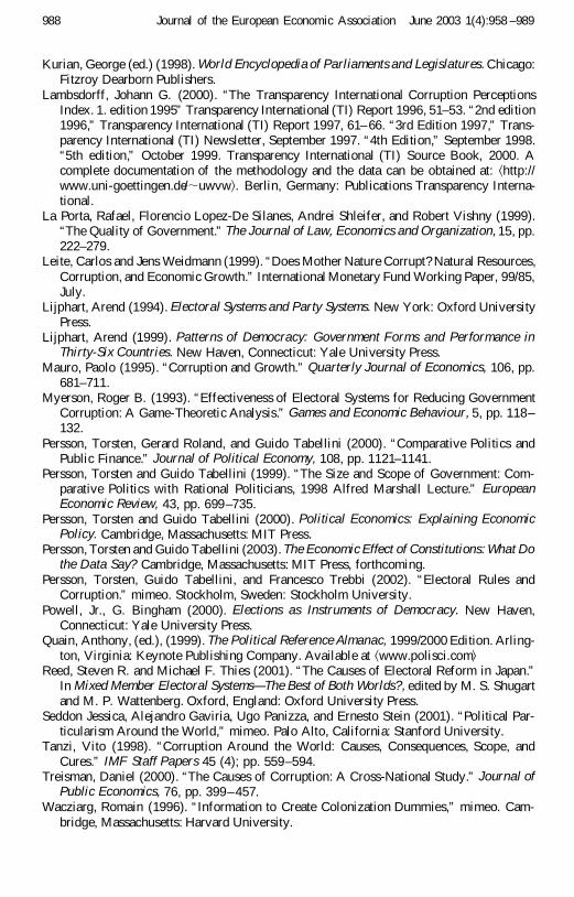
Kurian, George (ed.) (1998). World Encyclopedia of Parliaments and Legislatures. Chicago:Fitzroy Dearborn Publishers.

Lambsdorff, Johann G. (2000). “The Transparency International Corruption PerceptionsIndex. 1. edition 1995” Transparency International (TI) Report 1996, 51–53. “2nd edition1996,” Transparency International (TI) Report 1997, 61– 66. “3rd Edition 1997,” Trans-parency International (TI) Newsletter, September 1997. “4th Edition,” September 1998.“5th edition,” October 1999. Transparency International (TI) Source Book, 2000. Acomplete documentation of the methodology and the data can be obtained at: ^http://www.uni-goettingen.de/;uwvw&. Berlin, Germany: Publications Transparency Interna-tional.

La Porta, Rafael, Florencio Lopez-De Silanes, Andrei Shleifer, and Robert Vishny (1999).“The Quality of Government.” The Journal of Law, Economics and Organization, 15, pp.222–279.

Leite, Carlos and Jens Weidmann (1999). “Does Mother Nature Corrupt? Natural Resources,Corruption, and Economic Growth.” International Monetary Fund Working Paper, 99/85,July.

Lijphart, Arend (1994). Electoral Systems and Party Systems. New York: Oxford UniversityPress.

Lijphart, Arend (1999). Patterns of Democracy: Government Forms and Performance inThirty-Six Countries. New Haven, Connecticut: Yale University Press.

Mauro, Paolo (1995). “Corruption and Growth.” Quarterly Journal of Economics, 106, pp.681–711.

Myerson, Roger B. (1993). “Effectiveness of Electoral Systems for Reducing GovernmentCorruption: A Game-Theoretic Analysis.” Games and Economic Behaviour, 5, pp. 118–132.

Persson, Torsten, Gerard Roland, and Guido Tabellini (2000). “Comparative Politics andPublic Finance.” Journal of Political Economy, 108, pp. 1121–1141.

Persson, Torsten and Guido Tabellini (1999). “The Size and Scope of Government: Com-parative Politics with Rational Politicians, 1998 Alfred Marshall Lecture.” EuropeanEconomic Review, 43, pp. 699–735.

Persson, Torsten and Guido Tabellini (2000). Political Economics: Explaining EconomicPolicy. Cambridge, Massachusetts: MIT Press.

Persson, Torsten and Guido Tabellini (2003). The Economic Effect of Constitutions:What Dothe Data Say? Cambridge, Massachusetts: MIT Press, forthcoming.

Persson, Torsten, Guido Tabellini, and Francesco Trebbi (2002). “Electoral Rules andCorruption.” mimeo. Stockholm, Sweden: Stockholm University.

Powell, Jr., G. Bingham (2000). Elections as Instruments of Democracy. New Haven,Connecticut: Yale University Press.

Quain, Anthony, (ed.), (1999). The Political Reference Almanac, 1999/2000 Edition. Arling-ton, Virginia: Keynote Publishing Company. Available at ^www.polisci.com&

Reed, Steven R. and Michael F. Thies (2001). “The Causes of Electoral Reform in Japan.”In Mixed Member Electoral Systems—The Best of Both Worlds?, edited by M. S. Shugartand M. P. Wattenberg. Oxford, England: Oxford University Press.

Seddon Jessica, Alejandro Gaviria, Ugo Panizza, and Ernesto Stein (2001). “Political Par-ticularism Around the World,” mimeo. Palo Alto, California: Stanford University.

Tanzi, Vito (1998). “Corruption Around the World: Causes, Consequences, Scope, andCures.” IMF Staff Papers 45 (4); pp. 559–594.

Treisman, Daniel (2000). “The Causes of Corruption: A Cross-National Study.” Journal ofPublic Economics, 76, pp. 399–457.

Wacziarg, Romain (1996). “Information to Create Colonization Dummies,” mimeo. Cam-bridge, Massachusetts: Harvard University.


Wei, Shang-Jin (1997a). “How Taxing is Corruption on International Investors.” NBERWorking Paper 6030.

Wei, Shang-Jin (1997b). “Why is Corruption so Much More Taxing Than Tax? ArbitrarinessKills,” NBER Working Paper 6255.

World Bank (1997–1999). World Development Report. New York: Oxford University Press.Wooldridge, Jeffrey M. (2002). Econometric Analysis of Cross Section and Panel Data.

Cambridge, Massachusetts: MIT Press.


Documents

Electoral Rules and Corruption - Home | Projects at …projects.iq.harvard.edu/gov2126/files/person_tabellini...ELECTORAL RULES AND CORRUPTION Torsten Persson Stockholm University