Electoral Competition and Duverger’s Law

Alexey Sokolin

Submitted to the Department of Economics of Amherst College in partial fulfillment of the requirements for the degree of Bachelor of Arts with Honors.

Professor Frank Westhoff, Faculty Advisor

April 29, 2006

1

Acknowledgements

The thesis process has been one of remarkable challenge and learning, and I am very grateful

to the people who have helped me along the way. I would like to thank Professor Jessica Reyes for

encouraging open thinking and creativity, Professor Walter Nicholson for grounding my ideas and

connecting them to appropriate literature, and Professor Frank Westhoff for helping me bring my

model to fruition. Thanks also to the Amherst Economics department, for providing me with the

tools, imagination and motivation to pursue this project. Professor Geoffrey Woglom, my academic

advisor, has fueled my addiction to difficult material and the desire to improve myself intellectually.

I could not have finished this thesis without the support of my friends and their patience.

Specifically, I would like to thank Sam Maurer for reading the entire draft and making insightful

comments, and Tim Brooks Paige, for spending an absurd amount of time with me drawing diagrams

and confirming the logic of my arguments.

2

Table of Contents

1 Introduction……………………………………………………………………. 4 2 Literature Review……………………………………………………………… 6 2.0 The Downs Model……………………………………………………… 6 2.1 The Wittman Model……………………………………………………. 7

2.2 Uncertainty……………………………………………………………... 8 2.3 Multidimensionality and Probabilistic Voting…………………………… 9 2.4 Citizen-Candidate model and Entry…………………………………….. 10 2.5 Separation of Candidates and Parties…………………………………… 11

3 Model and Results……………………………………………………………... 12 3.0 Definitions…………………………………………………………….... 12 3.1 Two Parties: Unrestricted Budget, Utility from Payoffs………………… 15 3.2 Two Parties: Restricted Budget, Utility from Payoffs…………………… 17 3.3 Two Parties: Unrestricted Budget, Utility from Payoffs and Savings……. 20 3.4 Two Parties: Restricted Budget, Utility from Payoffs and Savings………. 28 3.5 Three Parties: Unrestricted Budget, Utility from Payoffs and Savings…… 35 3.6 Three Parties: Restricted Budget, Utility from Payoffs and Savings…….... 40 4 Entry……………………………………………………………………………. 43 5 Conclusion……………………………………………………………………… 45 6 Appendix……………………………………………………………………….. 46 6.0 Definition of Local Payoffs of Party 1 in a given district………………... 46 6.1 Definition of Payoffs, conditional………………………………………. 46 6.2 Definition of Payoffs, unconditional……………………………………. 47 6.3 Definition of Costs, conditional………………………………………… 47 6.4 Definition of Costs, unconditional……………………………………… 47 6.5 Definition of Utility from Savings, conditional………………………….. 48 7 Bibliography…………………………………………………………………… 49

3

1 – Introduction

The aim of this thesis is to explain the robustness of the two-party equilibrium prevalent in

the United States. In other words, why do third parties rarely enter national electoral competition,

and why do they almost never win? There are two points which make this question particularly

interesting. First, the two-party equilibrium has strong implications for policy formation: voter

welfare is not necessarily maximized when options are so limited. While having fewer political parties

likely leads to economies of scale, a larger spectrum of parties would result in more policy diversity,

satisfying more voters. Understanding the cause of the two-party result is informative for thinking

about maximizing voter welfare. Second, there is a discrepancy between the basic game-theoretical

model of electoral competition and reality. Unlike the prediction of that model, parties differentiate

their policies and do not simply appease the median voter.

Sociologist Maurice Duverger was the first to note that a first-past-the-post voting system

consistently yields two-party outcomes. His most robust claim, titled “Duverger’s Law”, is that a

plurality voting (first-past-the-post) system leads to domination of elections by two political parties.

Duverger also hypothesized that run-off majority voting and proportional representation lead to a multi-party

result (Duverger, 1963), however this idea is not as widely accepted.

Duverger explained his law through a mechanical effect and a psychological factor (Riker, 1982, p.

761). The mechanical effect is an empirical observation that third parties in elections end up more

underrepresented than anticipated. In other words, a third party receives a lower percentage of seats

in Congress than the percentage of votes it garnered. Rae (1971) and Sprague (1980) provide

evidence that this mechanical effect concept is correct. The psychological factor explains that voters

may abandon preferred parties to vote for second-preferred candidates, which may have a higher

chance of winning the election. Voters do not want to waste their votes. This and related concepts

have been rigorously explored by social choice theory, and formalized into the idea of strategic voting

by Cox (1997).

4

Multiple models have attempted to move beyond Duverger’s explanation. The two party

equilibrium has been justified using district composition, ideological candidates, presidentialism,

differing party and candidate incentives, and ethnic heterogeneity among others. Chhibber and

Kollman (1998) even propose that party number is influenced over time by changes in the

concentration of political and economic power. This paper builds upon relevant game theory

literature to formulate a model that mirrors national party competition over multiple districts. It

provides a rationale for the two-party equilibrium in a large country with a complex voting

mechanism like the United States, and reaffirms Duverger’s conclusion.

The organization is as follows: Chapter 2 provides a literature review that summarizes basic

models of electoral competition and entry. The most important revisions of these models are

discussed next, providing a conceptual grounding for the approach taken in this paper. In Chapter 3,

I develop my own model of electoral competition on a national scale, with parties that compete on a

continuum of districts. This is meant to mirror Senate elections in the United States. After discussing

definitions and assumptions, I explore various specifications of two-party competition using a

restricted and unrestricted party budget, as well as two different formulations of a party’s utility

function. One utility function is based simply on payoffs from winning elections, while the other

includes a utility from savings. Next, I examine the incentives of potential new entrants, focusing on

expected utility of this third party and the effects of entry on the incumbents. Lastly, I create a model

of entry which provides a rationale for Duverger’s Law.

5

2 – Literature Review

2.0 The Downs Model

The fundamental model of electoral competition was developed by Downs (1957), adopting

Hotelling’s spatial product competition model to explain policy formation. In a Downsian world,

political parties and candidates are synonymous, and are only interested in winning the election. They

seek to maximize the probability of victory and are not encumbered by other motivations. There

exists a continuum of voters with symmetric single-peaked1 preferences regarding a specific policy p,

where p Є [0, 1]. The range [0, 1] is a uni-dimensional policy space, on which voters are distributed, with

median voter preferring policy pm. Voters vote for policies closest to their “bliss point”. For example,

a voter with ideal p = .4 will prefer p = .2 over p = .8. It is assumed that parties have perfect

information regarding the distribution of voters.

Parties 1 and 2 decide to announce a policy pi that maximizes their payoff Πi. The payoff

function is just the probability of winning the election given p1 announced by party 1 and p2

announced by party 2:

Payoff of party 1: Π1(p1, p2) = P(p1, p2)

Payoff of party 2: Π2(p1, p2) = 1 – P(p1, p2)

P(p1, p2) is probability that party 1 wins

The players competing in Downs will play any political position necessary to win the election. Each

will choose pi such that pi is a Condorcet winner, defined as a policy that “can beat all others … in a

series of pairwise majority votes” (Heap et al, 1992, p.301). In other words a Condorcet winner

policy p* can defeat or tie any other policy p ≠ p*. The Downs political equilibrium is thus policy

pair (p*, p*), where p* = pm. Both parties converge towards the preferred policy of the median voter,

1 A function is single peaked if it possesses a unique local maximum. This concept is explained in Roemer (2001, p.20).

6

and the election is a tie. By definition, a candidate wins a tie with probability 1/2. No profitable

deviation is available for either player, since a move away from pm will mean certain loss for the

diverging party.

The Downs result is elegant but not realistic. It has since been amended for ideological

motivations, multiple policy issues, uncertainty regarding voter behavior, as well as various other

issues. This paper’s model will feature a pure Downs competition in one of the stages of the national

electoral competition game. It is important to remember that Downs candidates converge to the

median to win the election, and split the payoff with probability 1/2 at equilibrium (pm, pm).

2.1 The Wittman Model (Ideological Candidates)

One of the primary criticisms of the Downs model is its limited representation of the true

motivations of political parties. In reality, politicians are usually partisan and likely care about what

policy is implemented. Wittman’s (1977) model uses a payoff function that incorporates both

probability of winning and utility gained from a specific policy. The payoff functions are below:

Payoff of party 1: Π1(p1,p2) = P(p1, p2) U1(p1) + (1 - P(p1, p2)) U1(p2)

Payoff of party 2: Π2(p1,p2) = P(p1, p2) U2(p1) + (1 - P(p1, p2)) U2(p2)

P(p1, p2) is probability that party 1 wins and p1 is played

Ui(pj) – utility of party i from policy j

Utility functions U1 and U2 represent policy preferences of the party leaders, which can also be

conceptualized as ideological citizen-candidates. These leaders have some ideological bliss point pibliss

where Ui is maximized. Persson and Tabellini (2000, p. 98) separate the payoff function into centrifugal

and centripetal forces. The centrifugal force pulls the party towards the ideological bliss point; the

centripetal force pushes the party towards the median pm in order to increase the probability of

winning. Despite this tension, the Wittman model has the same convergent Nash equilibrium

7

(p* = pm, p* = pm) as before. This is because the centripetal force dominates as a result of the

winner-takes-all formulation: if party 1 does not play the median and the other party does, party 1

will receive a payoff of U1(p2 = pm). If both parties play the median, party 1 receives the same payoff:

1/2(U1(pm) + 1/2(U1(pm) = U1(pm). Therefore, the parties will both edge closer to pm until they

converge; afterwards there is no incentive to diverge.

While Wittman’s original formulation does not lead to divergence, it is possible to amend

slightly the rationale behind the model to achieve differentiated policy. Instead of winner-takes-all,

consider a situation when a party can achieve some payoff even if the other party is closer to the

median. This type of payoff function would reflect Congressional elections. The centripetal force no

longer dictates discontinuous payoffs, and a meaningful tension can be explored between the desire

to win more votes and to stay true to ideology. The model in this paper explores a similar dynamic,

defining the centrifugal force as the desire to save money, rather than Wittman’s ideological

preferences.

2.2 Uncertainty

In reality, political parties do not have perfect information regarding the distribution of

voters. Campaigning and media efforts need to be used by politicians to understand voter

preferences and accurately position themselves. Roemer (2001) proposes models of uncertainty that

can be applied to Downs and Wittman: the state-space approach and the error-distribution model.

These models formulate uncertainty on a “macro” level, rather than tracking it in individual

preferences. The state space model essentially portrays a number of states of nature, occurring under

some probability distribution. These states of nature differ in voter behavior, resulting from some

exogenous shock such as bad weather, or political debates gone awry. Given these circumstances, in

some of states of nature policy p1 defeats policy p2, and in others p2 defeats p1. The probability of

party 1’s victory is the probability of a state of nature occurring in which p1 defeats p2. The second

approach to uncertainty, the error-distribution model, focuses instead on the candidates’ knowledge

8

of voters’ preferences. The political actors are imperfectly aware of the voter distribution, predicting

the fraction of voters that prefer to p1 to p2 with some margin of error.

Uncertainty is useful because it is more realistic and can induce divergent equilibria. Roemer

(2001) shows that Downs remains unaffected by uncertainty and the two parties continue to

converge. Wittman’s partisan politicians model, on the other hand, achieves differentiated equilibria

under either uncertainty approach. While the model in this paper does not directly introduce

uncertainty into party decision making, it nonetheless relies on something like the state space

approach. It will be shown that a third party faces uncertainty regarding how much money it can

fundraise, which in turn significantly affects its incentives.

2.3 Multidimensionality and Probabilistic Voting

So far, parties have been portrayed as competing over a single issue. Yet, legislatures do not

only consider issues of “left” and “right”, but those on multiple ideological levels: tax policy, foreign

relations, social welfare, among many others. It is possible to have different individual rankings for

multiple policy proposals of political candidates, making the voting decision more complicated.

Multidimensional policy competition attempts to model this situation.2. Unfortunately, it is very

difficult to find an equilibrium given multiple dimensions. The condition required for some policy to

be a Condorcet winner is prohibitively strong – it must be a “median in all directions”, requiring

extreme symmetry in the distribution of bliss points (Persson and Tabellini, 2000, p.29). Heap et al

(1992, p.223) explain: “the distribution must be such that one voter occupies the median of both

dimensions, and remaining voters are strung out in such a way that they are all diametrically opposed

to one another around this median point and exactly paired with one another”. The probability of

this scenario is nonexistent. The lack of an equilibrium leads to cycling, which means that a candidate

may always propose a policy that defeats the original, and there is no best response policy available

for any of the players. Both the Downs and Wittman model lack a stable equilibrium in this

2 Multidimensional policy competition is covered in Heap et al (1992, p.223), Persson and Tabellini (2000, p.29) and Roemer (2001, p.111).

9

formulation (Roemer, 2001). Probabilistic voting models, pioneered by Hinich (1977) and Coughlin and

Nitzan (1981) are used to find equilibria in multiple dimensions. By introducing uncertainty into

voter behavior, probabilistic voting makes the probability of a voter choosing a particular candidate

into a continuous function, fixing the discontinuities inherent in multidimensional competition.3

2.4 Citizen Candidate model and Entry

The citizen-candidate model, developed by Osborne and Slivinksi (1996) and Besley and

Coate (1997), is the starting point for analyzing the incentives candidates face when entering an

election. Each candidate has a particular bliss-point, is motivated by both probability of winning and

policy implemented. There are multiple feasible Nash equilibria, including single candidate and multi-

candidate equilibria (Persson and Tabellini, 2000, 104). Essentially, a voter enters the electoral

competition if the gain in utility from implementing her preferred policy over the incumbent policy is

greater than the cost of entry. One relevant pitfall of this model is the absence of established players

prior to the entry calculus.

Other entry models have been developed by Palfrey (1984), Feddersen, Sened and Wright

(1990) and Shvetsova (1995). In general, most models show that a third party is unlikely to compete

in the election given positive entry cost, as predicted by Duverger. Palfrey (1984) finds a non-centrist

equilibrium where the incumbents win with probability 1/2. The intuition is as follows: if parties 1

and 2 play p1 < pm and p2 < pm, then party 3 can steal the election by playing p3 = pm. Thus p1 and p2

are on opposite sides of the median. If the third party would only enter if there is positive probability

of victory, it does not enter because cost is too high and the incumbents face the regular Downs

game. If the third party enters even if it bound to lose, p1 and p2 do not converge in order to protect

their flank – a third party could come from the side, capturing votes and causing the opposite

incumbent to win. Callander (1999, p.19) extends Palfrey’s model to include a continuum of districts

across which parties choose a single policy, also finding a unique non-centrist two-party equilibrium.

3 The discussion of probabilistic voting by Persson and Tabellini (2000, p. 33) is particularly apt.

10

Feddersen et al (1990) model another approach to the entry decision. Citizens vote

strategically, and the cost of entry is α The payoff function is simply the probability of winning times

the utility gained from playing a preferred policy [Pi(pi)Ui(pi)]. Given simplifying assumptions, Pi(pi) =

1/n in equilibrium, n being the number of entrants. The entry decision Pi(pi)Ui(pi) > α can be

represented as Ui(pi)/α > n; in other words the benefit-cost ratio for the given election must exceed

the number of candidates. The model in my paper uses multiple concepts discussed in this section,

such as entry cost, the utility of victory and the desire of parties to protect their flanks.

2.5 Separation of candidates and parties

Recent work on electoral competition looks closer at the incentives of the different actors in

the political game. Specifically, models can be made more realistic by separating the concept of

“political party” from that of “candidate”. Eyster and Kittsteiner (2004) propose a novel approach to

finding a non-centrist equilibrium. They separate political actors into parties that set a policy across

multiple districts in the first round of the game, and local candidates that deviate from their party’s

policy in the second round. The districts have different distributions of voters, and therefore

different local median policies. The candidates are Downs-motivated to win the local election, and

move towards that local median at a cost. This cost represents “advertising a new policy …

unpalatable payments or promises to special interests necessary to finance publicizing a change from

party policy” (Eyster and Kittsteiner, 2004, p.4). The payoff function for the parties balances the

probability of winning the national election against the campaign costs incurred by the candidates.

Maximizing this function leads parties to diverge in policy and decrease direct competition. The

model offers a historically feasible result using an elegant qualification of Downs and is the starting

point for the specification used in this paper.

11

3 – Model and Results

3.0 Definitions

Two parties, party 1 and party 2, compete in a national election with a continuum of districts

uniformly distributed on the uni-dimensional national policy space [0, 1]. The preferred median

policy pmlocal of each district is the location of that district on the national policy space. The parties

announce national policies p1 and p2. In each of the districts, local candidates compete in a Downsian

election. This implies that local candidates must converge to the pmlocal to maximize the chance of

victory. The candidates start out at the national policy positions of their parties (p1, p2). The

candidates’ move to a local median is costly for the party. If a candidate can credibly represent the

national party in a district, the national party finances this move. Some districts are so far away from

a party’s position that its candidate cannot credibly represent the party in that district, and the party

does not field a candidate. In other words, the candidate would move so far away from the party on

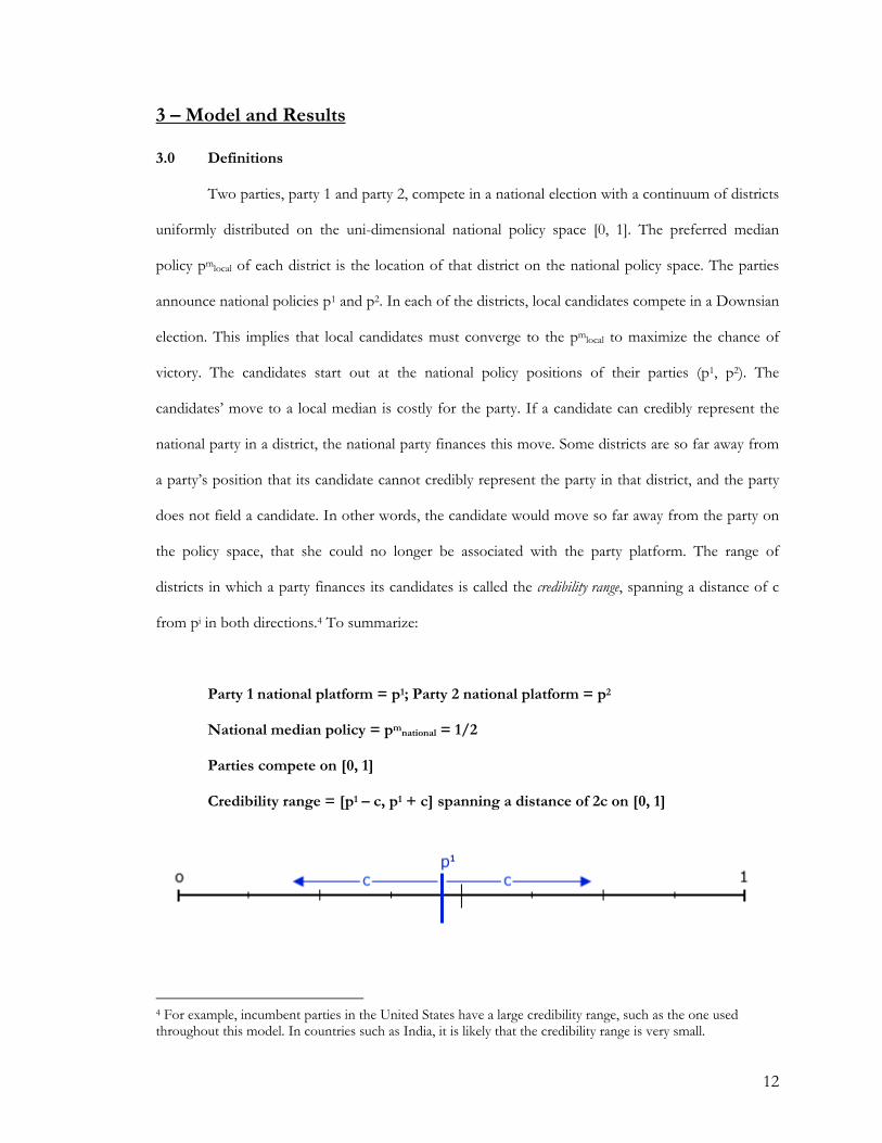
the policy space, that she could no longer be associated with the party platform. The range of

districts in which a party finances its candidates is called the credibility range, spanning a distance of c

from pi in both directions.4 To summarize:

Party 1 national platform = p1; Party 2 national platform = p2

National median policy = pmnational = 1/2

Parties compete on [0, 1]

Credibility range = [p1 – c, p1 + c] spanning a distance of 2c on [0, 1]

4 For example, incumbent parties in the United States have a large credibility range, such as the one used throughout this model. In countries such as India, it is likely that the credibility range is very small.

12

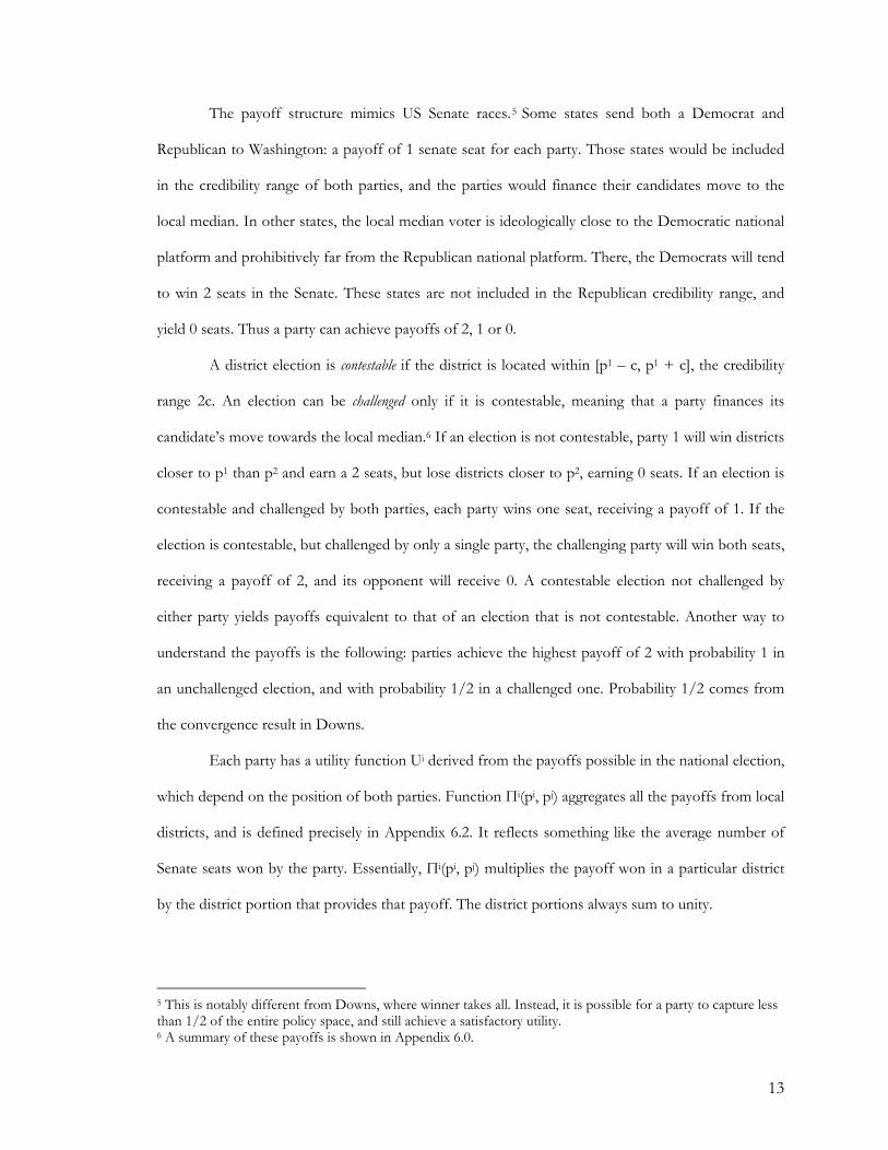
The payoff structure mimics US Senate races.5 Some states send both a Democrat and

Republican to Washington: a payoff of 1 senate seat for each party. Those states would be included

in the credibility range of both parties, and the parties would finance their candidates move to the

local median. In other states, the local median voter is ideologically close to the Democratic national

platform and prohibitively far from the Republican national platform. There, the Democrats will tend

to win 2 seats in the Senate. These states are not included in the Republican credibility range, and

yield 0 seats. Thus a party can achieve payoffs of 2, 1 or 0.

A district election is contestable if the district is located within [p1 – c, p1 + c], the credibility

range 2c. An election can be challenged only if it is contestable, meaning that a party finances its

candidate’s move towards the local median.6 If an election is not contestable, party 1 will win districts

closer to p1 than p2 and earn a 2 seats, but lose districts closer to p2, earning 0 seats. If an election is

contestable and challenged by both parties, each party wins one seat, receiving a payoff of 1. If the

election is contestable, but challenged by only a single party, the challenging party will win both seats,

receiving a payoff of 2, and its opponent will receive 0. A contestable election not challenged by

either party yields payoffs equivalent to that of an election that is not contestable. Another way to

understand the payoffs is the following: parties achieve the highest payoff of 2 with probability 1 in

an unchallenged election, and with probability 1/2 in a challenged one. Probability 1/2 comes from

the convergence result in Downs.

Each party has a utility function Ui derived from the payoffs possible in the national election,

which depend on the position of both parties. Function Πi(pi, pj) aggregates all the payoffs from local

districts, and is defined precisely in Appendix 6.2. It reflects something like the average number of

Senate seats won by the party. Essentially, Πi(pi, pj) multiplies the payoff won in a particular district

by the district portion that provides that payoff. The district portions always sum to unity.

5 This is notably different from Downs, where winner takes all. Instead, it is possible for a party to capture less than 1/2 of the entire policy space, and still achieve a satisfactory utility. 6 A summary of these payoffs is shown in Appendix 6.0.

13

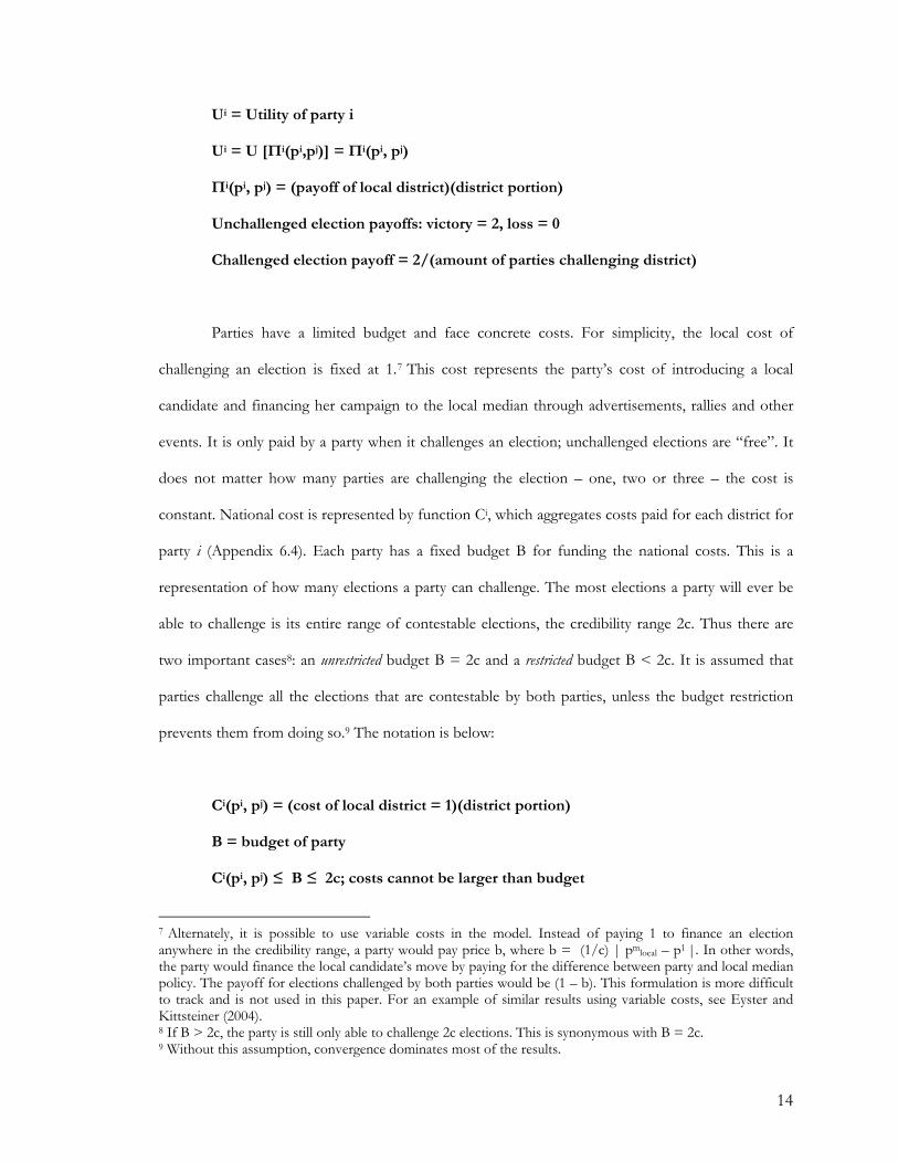
Ui = Utility of party i

Ui = U [Πi(pi,pj)] = Πi(pi, pj)

Πi(pi, pj) = (payoff of local district)(district portion)

Unchallenged election payoffs: victory = 2, loss = 0

Challenged election payoff = 2/(amount of parties challenging district)

Parties have a limited budget and face concrete costs. For simplicity, the local cost of

challenging an election is fixed at 1.7 This cost represents the party’s cost of introducing a local

candidate and financing her campaign to the local median through advertisements, rallies and other

events. It is only paid by a party when it challenges an election; unchallenged elections are “free”. It

does not matter how many parties are challenging the election – one, two or three – the cost is

constant. National cost is represented by function Ci, which aggregates costs paid for each district for

party i (Appendix 6.4). Each party has a fixed budget B for funding the national costs. This is a

representation of how many elections a party can challenge. The most elections a party will ever be

able to challenge is its entire range of contestable elections, the credibility range 2c. Thus there are

two important cases8: an unrestricted budget B = 2c and a restricted budget B < 2c. It is assumed that

parties challenge all the elections that are contestable by both parties, unless the budget restriction

prevents them from doing so.9 The notation is below:

Ci(pi, pj) = (cost of local district = 1)(district portion)

B = budget of party

Ci(pi, pj) ≤ B ≤ 2c; costs cannot be larger than budget

7 Alternately, it is possible to use variable costs in the model. Instead of paying 1 to finance an election anywhere in the credibility range, a party would pay price b, where b = (1/c) | pmlocal – p1 |. In other words, the party would finance the local candidate’s move by paying for the difference between party and local median policy. The payoff for elections challenged by both parties would be (1 – b). This formulation is more difficult to track and is not used in this paper. For an example of similar results using variable costs, see Eyster and Kittsteiner (2004). 8 If B > 2c, the party is still only able to challenge 2c elections. This is synonymous with B = 2c. 9 Without this assumption, convergence dominates most of the results.

14

The sections below explore a number of permutations of the defined model given 2c = 1/2.

First, I look for a two-party equilibrium using Ui = Πi(pi, pj) and an unrestricted budget B = 2c. This

formulation leads to convergence of the two parties at the national median. In the next section the

budget is restricted to B = c in order to simulate fundraising limits. Convergence dominates again,

but I find a budgeting strategy that is useful for later sections. Section 3.3 amends function Ui to

include utility from saving the budget, which reflects diminishing marginal utility of money. As a

result, the parties are pushed apart by their desire to save and a set of divergent equilibria with a fixed

distance between parties becomes possible. Section 3.4 explores the effect of a budget restriction on

the new utility function, showing that the distance between parties’ policy locations is inversely

affected by the size of the budget. A larger budget allows parties to play policies closer together, a

smaller budget forces parties to diverge more extremely. Sections 3.5 and 3.6 explore the expected

payoffs of a third party entrant into the equilibria previously found. In 3.5 the entrant’s budget is

equal to that of the incumbents, while in 3.6, the third party’s budget is restricted and the maximum

utility is consequently smaller. Lastly, I develop a model of entry for the third party which shows why

new entrants are extremely rare and Duverger’s Law holds.

3.1 Two Party Model: Unrestricted Budget, Utility from Payoffs

Consider the example where B = 2c, c = 1/4. There is no real budget constraint. All

contestable elections are potentially challenged. Diagrams on the next page provide an easier method

to track payoffs from votes and costs than the definitions of Πi(pi,pj) and Ci in the Appendix. The

vertical axis represents possible payoffs from a local district on range [0, 2] and the horizontal axis is

the national policy space [0, 1]. The blue area is Π1, the aggregate of payoffs for party 1 or the

number of Senate seats captured. Similarly the red area is Π2, the aggregate of payoffs for party 2 or

the number of Senate seats captured by party 2. The areas are calculated by multiplying the local

district payoff times the district portion with that payoff. For example, Π1 = (2)(unchallenged

districts of party 1) + 1(challenged districts by both parties) + 0(unchallenged districts of party 2). In

15

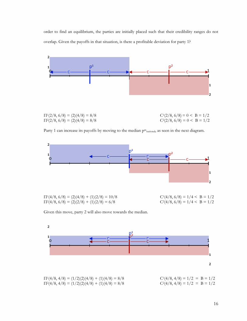
order to find an equilibrium, the parties are initially placed such that their credibility ranges do not

overlap. Given the payoffs in that situation, is there a profitable deviation for party 1?

Π1(2/8, 6/8) = (2)(4/8) = 8/8 C1(2/8, 6/8) = 0 < B = 1/2 Π2(2/8, 6/8) = (2)(4/8) = 8/8 C2(2/8, 6/8) = 0 < B = 1/2 Party 1 can increase its payoffs by moving to the median pmnational, as seen in the next diagram.

Π1(4/8, 6/8) = (2)(4/8) + (1)(2/8) = 10/8 C1(4/8, 6/8) = 1/4 < B = 1/2 Π2(4/8, 6/8) = (2)(2/8) + (1)(2/8) = 6/8 C2(4/8, 6/8) = 1/4 < B = 1/2 Given this move, party 2 will also move towards the median.

Π1(4/8, 4/8) = (1/2)(2)(4/8) + (1)(4/8) = 8/8 C1(4/8, 4/8) = 1/2 = B = 1/2 Π2(4/8, 4/8) = (1/2)(2)(4/8) + (1)(4/8) = 8/8 C2(4/8, 4/8) = 1/2 = B = 1/2

16

Once both parties converge to pmnational there are no profitable deviations for either party. The

equilibrium is (1/2, 1/2). The two parties compete over their entire credibility range for a payoff of 1,

and gain a payoff of 2 from all the other districts with probability 1/2. This result is equivalent to

Downs. Next I test the possibility that limits on fundraising could lead to divergence.

3.2 Two Party Model: Restricted Budget, Utility from Payoffs

In the above example, parties could afford to challenge all the elections in the credibility

range. Here the budget is limited to reflect campaign-finance legislation, or simply smaller budgets

resulting from poor fundraising. For example, let B = 1c, c = 1/4. It is assumed that both parties are

equally affected by the restriction. Another step is introduced into the electoral competition game.

First, the party decides which policy to play, then it decides which contestable elections it will

challenge. Does this constraint affect the locations of the national policies? Starting at equilibrium (p1

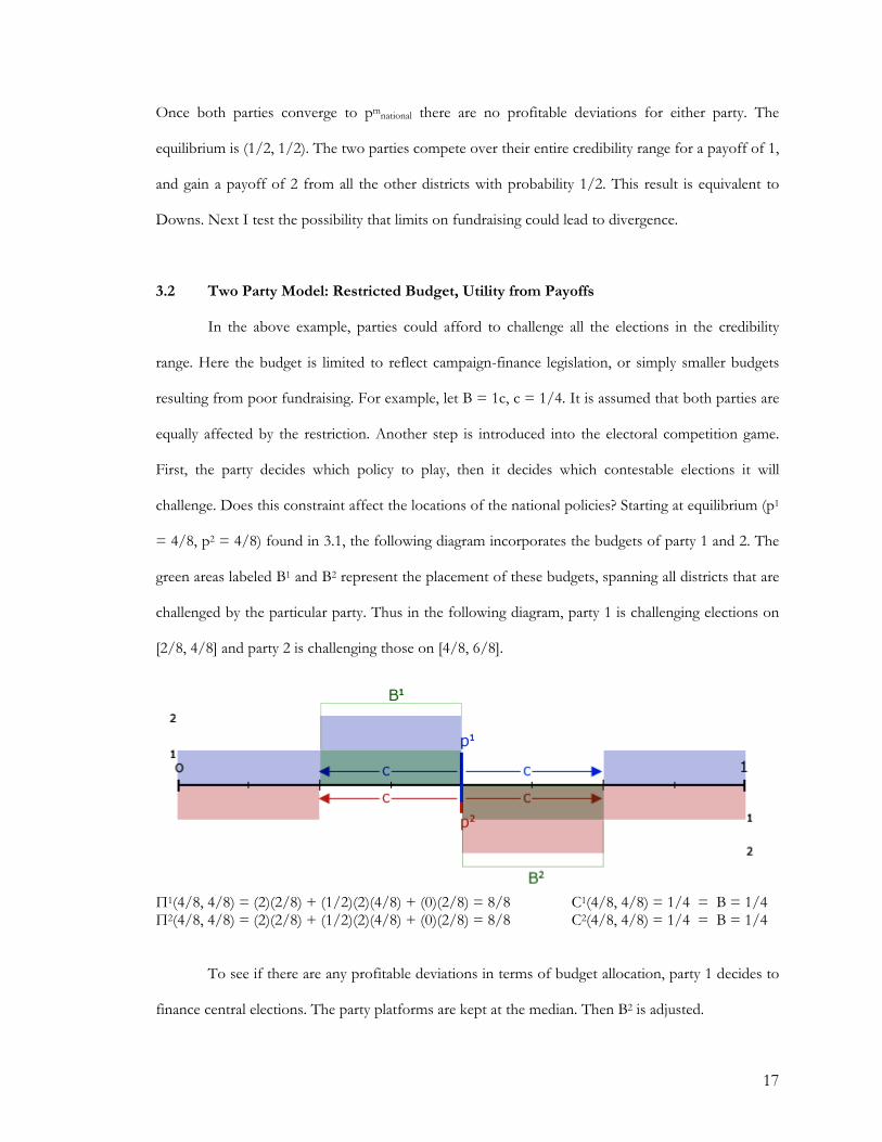
= 4/8, p2 = 4/8) found in 3.1, the following diagram incorporates the budgets of party 1 and 2. The

green areas labeled B1 and B2 represent the placement of these budgets, spanning all districts that are

challenged by the particular party. Thus in the following diagram, party 1 is challenging elections on

[2/8, 4/8] and party 2 is challenging those on [4/8, 6/8].

Π1(4/8, 4/8) = (2)(2/8) + (1/2)(2)(4/8) + (0)(2/8) = 8/8 C1(4/8, 4/8) = 1/4 = B = 1/4 Π2(4/8, 4/8) = (2)(2/8) + (1/2)(2)(4/8) + (0)(2/8) = 8/8 C2(4/8, 4/8) = 1/4 = B = 1/4

To see if there are any profitable deviations in terms of budget allocation, party 1 decides to

finance central elections. The party platforms are kept at the median. Then B2 is adjusted.

17

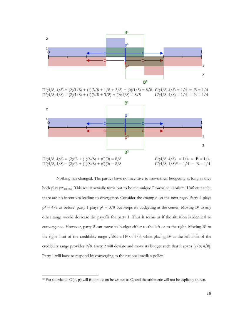
Π1(4/8, 4/8) = (2)(1/8) + (1)(3/8 + 1/8 + 2/8) + (0)(1/8) = 8/8 C1(4/8, 4/8) = 1/4 = B = 1/4 Π2(4/8, 4/8) = (2)(1/8) + (1)(3/8 + 3/8) + (0)(1/8) = 8/8 C2(4/8, 4/8) = 1/4 = B = 1/4

Π1(4/8, 4/8) = (2)(0) + (1)(8/8) + (0)(0) = 8/8 C1(4/8, 4/8) = 1/4 = B = 1/4 Π2(4/8, 4/8) = (2)(0) + (1)(8/8) + (0)(0) = 8/8 C2(4/8, 4/8)10 = 1/4 = B = 1/4

Nothing has changed. The parties have no incentive to move their budgeting as long as they

both play pmnational. This result actually turns out to be the unique Downs equilibrium. Unfortunately,

there are no incentives leading to divergence. Consider the example on the next page. Party 2 plays

p2 = 4/8 as before; party 1 plays p1 = 3/8 but keeps its budgeting at the center. Moving B1 to any

other range would decrease the payoffs for party 1. Thus it seems as if the situation is identical to

convergence. However, party 2 can move its budget either to the left or to the right. Moving B2 to

the right limit of the credibility range yields a Π2 of 7/8, while placing B2 at the left limit of the

credibility range provides 9/8. Party 2 will deviate and move its budget such that it spans [2/8, 4/8].

Party 1 will have to respond by converging to the national median policy.

10 For shorthand, Ci(pi, pj) will from now on be written as Ci, and the arithmetic will not be explicitly shown.

18

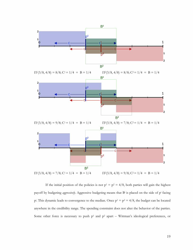
Π1(3/8, 4/8) = 8/8; C1 = 1/4 = B = 1/4 Π2(3/8, 4/8) = 8/8; C2 = 1/4 = B = 1/4

Π1(3/8, 4/8) = 9/8; C1 = 1/4 = B = 1/4 Π2(3/8, 4/8) = 7/8; C2 = 1/4 = B = 1/4

Π1(3/8, 4/8) = 7/8; C1 = 1/4 = B = 1/4 Π2(3/8, 4/8) = 9/8; C2 = 1/4 = B = 1/4

If the initial position of the policies is not p1 = p2 = 4/8, both parties will gain the highest

payoff by budgeting aggressively. Aggressive budgeting means that Bi is placed on the side of pi facing

pj. This dynamic leads to convergence to the median. Once p1 = p2 = 4/8, the budget can be located

anywhere in the credibility range. The spending constraint does not alter the behavior of the parties.

Some other force is necessary to push p1 and p2 apart – Wittman’s ideological preferences, or

19

disutility from spending the entire budget (Eyster and Kittsteiner, 2004), which is used in the next

section.

3.3 Two Party Model: Unrestricted Budget, Utility from Payoffs and Money

Political parties care about more than just winning elections. Consider campaign finance –

the assumption that the party is indifferent between spending the entire budget and saving money is

unrealistic. Rather, a party is likely to receive utility from unspent money because it can use that

money to finance other projects. These projects would not be related to electoral competition. For

example, sponsoring events that bring district representatives together and create unity within the

party is likely to make governance more effective. Saved money can also be used to lobby and to

affect issues that cannot be resolved in the legislative branch. To reflect the party’s incentives

regarding budget spending, this section amends the utility function to include utility gained by parties

from saving money (V(Si)). Given this new utility function, I find a set of divergent two-party

equilibria. It will be shown that depending on a party’s marginal utility of saved money, a party will

desire to save some fixed amount no matter where its opponent is located. In order to save this

amount, the party will move a given distance away from its opponent’s policy position.

Function Si stands for savings, which is B minus the costs of financing elections. V is the

utility function that indicates how much utility a party receives from Si, defined as (Si)1/x, where 1/x is

an arbitrary rate. A specific formulation of V is used in this paper to find equilibria: x = 2 and V =

(Si)1/2. This function reflects diminishing marginal returns from holding money – each additional

dollar saved yields less utility. There is now a tension in the party’s policy decision: financing

elections decreases the totally utility of the party, while winning elections increases that utility. The

relevant redefinitions are below11:

11 It is possible to assign weights to Πi(pi,pj) and V(Si) in the utility function: Ui = a(Πi) + b(V(Si)). However, it is assumed that a = b = 1 for simplicity. Intuitively, it can be seen that if a > b, parties will desire to come closer together; if a < b, parties will wish to move apart and increase savings beyond the result found in this section.

20

Ui = U [Πi(pi,pj), Di] = Πi(pi, pj) + V(Si)

Si = (B – Ci(pi, pj))

V(Si) = (Si)1/x; x = 2 unless stated otherwise

δUi/ δSi > 0

Ci(pi, pj) ≤ B = 2c

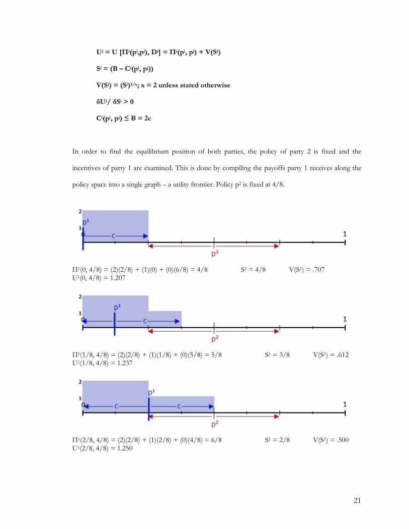
In order to find the equilibrium position of both parties, the policy of party 2 is fixed and the

incentives of party 1 are examined. This is done by compiling the payoffs party 1 receives along the

policy space into a single graph – a utility frontier. Policy p2 is fixed at 4/8.

Π1(0, 4/8) = (2)(2/8) + (1)(0) + (0)(6/8) = 4/8 S1 = 4/8 V(S1) = .707 U1(0, 4/8) = 1.207

Π1(1/8, 4/8) = (2)(2/8) + (1)(1/8) + (0)(5/8) = 5/8 S1 = 3/8 V(S1) = .612 U1(1/8, 4/8) = 1.237

Π1(2/8, 4/8) = (2)(2/8) + (1)(2/8) + (0)(4/8) = 6/8 S1 = 2/8 V(S1) = .500 U1(2/8, 4/8) = 1.250

21

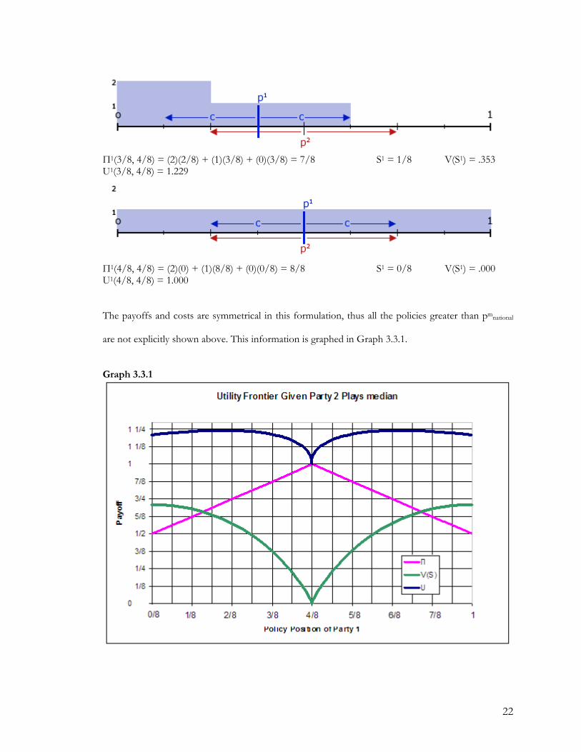
Π1(3/8, 4/8) = (2)(2/8) + (1)(3/8) + (0)(3/8) = 7/8 S1 = 1/8 V(S1) = .353 U1(3/8, 4/8) = 1.229

Π1(4/8, 4/8) = (2)(0) + (1)(8/8) + (0)(0/8) = 8/8 S1 = 0/8 V(S1) = .000 U1(4/8, 4/8) = 1.000

The payoffs and costs are symmetrical in this formulation, thus all the policies greater than pmnational

are not explicitly shown above. This information is graphed in Graph 3.3.1.

Graph 3.3.1

22

The utility function U can be seen to approximately reach a maximum at 2/8 in graph 3.3.1.

A more precise way to find a solution is to differentiate the utility function with respect to the policy

of party 1. It is possible to use definitions 6.1 and 6.5 in the appendix because c is sufficiently small.

In this example so far p1 < p2, therefore there are two situations: that of competition due to both

parties challenging elections (p1 + 2c > p2) and that of non-competition (p1 + 2c < p2). The case of

non-competition is trivial, possible only at p1 = 0/8, because the utility reached is significantly smaller

than when both parties challenge. Therefore, Π1 = p1 + p2 and V(S1) = (B – p1 + p2 – 2c)1/2.

Π1(p1, 1/2) = p1 + 1/2

V(S1) = (1/2 – p1 + 1/2 – 1/2)1/2 = (1/2 – p1)1/2

U1 = p1 + 1/2 + (1/2 – p1)1/2

To find a local maximum, set δU1/δp1 equal to zero:

δ[p1 + 1/2 + (1/2 – p1)1/2]/δp1 = 0 1 + 0 + 1/2(1/2 – p1)-1/2(-1) = 0

2 = – (1/2 – p1)-1/2 4 = 1/(1/2 – p1) 1/4 = 1/2 – p1 p1 = 2/8

Party 1 locates p1 at 2/8, or symmetrically at 6/8, on the national policy space. Either of these

locations will yield the highest possible payoff given that p2 = 4/8. The distance between p1 and p2 is

1/4. This distance allows both parties to save a total of 1/4 each, which is exactly where the V

function reaches a slope of -1. The point at which V has a slope of -1 is important because Π has a

slope of 1, and thus the U function has slope = 0. To double check the accuracy of this 1/4 savings,

I set δV(S1)/δp1 to 1.

δ[(p2 – p1)1/2]/δp1 = -1 1/2(p2 – p1)-1/2 = 1 (p2 – p1)1/2 = 1/2

(p2 – p1) = 1/4

23

In the case of p1 > p2, V(S1) equals (B – p2 + p1 – 2c)1/2. This function has slope 1, counteracting

slope -1 of Π1, also when the distance between parties is 1/4:

δ[(-p2 + p1)1/2]/δp1 = 1 1/2(-p2 + p1)-1/2 = 1 (-p2 + p1)1/2 = 1/2

(p1 – p2) = ¼

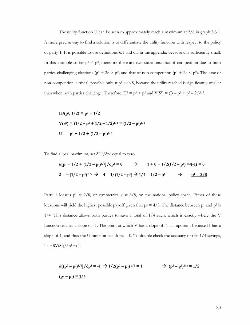
Given party 1’s move, how does party 2 respond? I examine the response of the opponent to pi =

6/8, which is the utility maximizing position of party 1 in the previous example, hoping to find an

equilibrium at policy pair (4/8, 6/8). The locations of the parties are switched to keep the “fixed”

party the same, thereby keeping the solution on the same side.

Π1(0, 6/8) = (2)(3/8) + (1)(0) + (0)(5/8) = 6/8 S1 = 4/8 V(S1) = .707 U1(0, 6/8) = 1.457

Π1(2/8, 6/8) = (2)(4/8) + (1)(0) + (0)(4/8) = 8/8 S1 = 4/8 V(S1) = .707 U1(2/8, 6/8) = 1.707

Π1(4/8, 6/8) = (2)(4/8) + (1)(2/8) + (0)(2/8) = 10/8 S1 = 2/8 V(S1) = .5 U1(4/8, 6/8) = 1.750

24

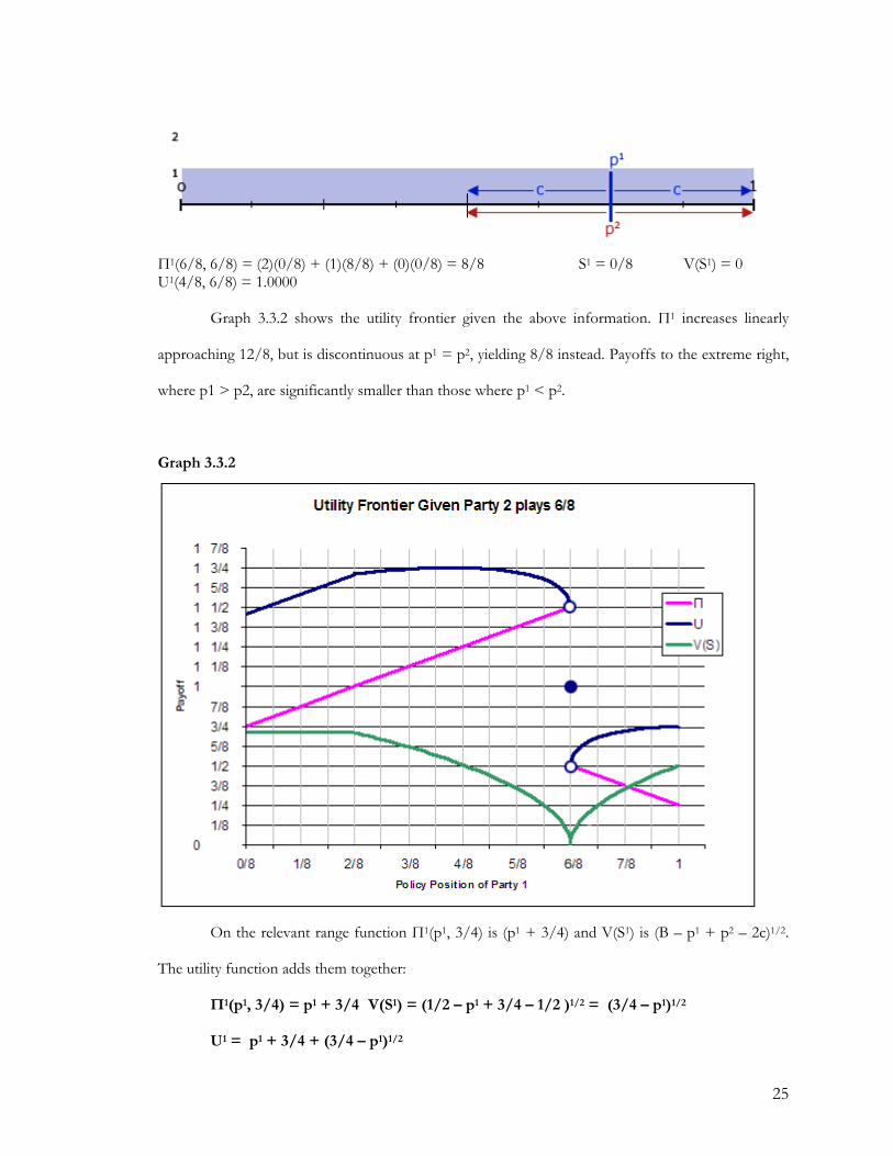
Π1(6/8, 6/8) = (2)(0/8) + (1)(8/8) + (0)(0/8) = 8/8 S1 = 0/8 V(S1) = 0 U1(4/8, 6/8) = 1.0000 Graph 3.3.2 shows the utility frontier given the above information. Π1 increases linearly

approaching 12/8, but is discontinuous at p1 = p2, yielding 8/8 instead. Payoffs to the extreme right,

where p1 > p2, are significantly smaller than those where p1 < p2.

Graph 3.3.2 On the relevant range function Π1(p1, 3/4) is (p1 + 3/4) and V(S1) is (B – p1 + p2 – 2c)1/2.

The utility function adds them together:

Π1(p1, 3/4) = p1 + 3/4 V(S1) = (1/2 – p1 + 3/4 – 1/2 )1/2 = (3/4 – p1)1/2

U1 = p1 + 3/4 + (3/4 – p1)1/2

25

To find the maximum, set δU1/ δp1 equal to zero.

δ[p1 + 3/4 + (3/4 – p1)1/2]/δp1 = 0 1 + 0 + 1/2(3/4 – p1)-1/2(-1)= 0

2 = (3/4 – p1)-1/2 4 = 1/(3/4 – p1) 1/4 = 3/4 – p1 p1 = 4/8

When party 2 plays p2 = 6/8, party 1’s best response is to play the median p1 = 4/8. As before,

parties wish to achieve S1 = 1/4, moving apart a distance of 1/4 . The asymmetric policy pair (4/8,

6/8) is a stable equilibrium. Similarly, other equilibria with the distance of 1/4 between the two party

policies are equilibria, including (2/8, 4/8), (6/8, 4/8) and the symmetric equilibrium (3/8, 5/8).

The above example allowed us to find how much parties wish to save given x = 2 and an

unrestricted budget B = 2c. Below, I generalize the result for all values of x.

If p1 > p2

Π1(p1,p2) = 2 – (p1 + p2)

V(S1) = ((B – 2c) + p1 – p2)1/x

U1 = 2 – (p1 + p2) + (p1 – p2)1/x

δ[2–(p1 + p2)+(p1 – p2)1/x]/δp1 = 0

0 – 1 – 0 + (1/x)( p1 – p2)(1/x – x/x) = 0

1 = (1/x)(p1 – p2)(1/x – x/x)

x = (p1 – p2)((1 –x)/x)

x(x/(1 – x)) = (p1 – p2)

-p1 + x(x/(1 – x)) = -p2

p1 = p2 + x(x/(1– x))

If p1 < p2

Π1(p1,p2) = p1 + p2

V(S1) = ((B – 2c) + p2 – p1)1/x

U1 = p1 + p2 + (p2 – p1)1/x

δ[ p1 + p2 + (p2 – p1)1/x ] / δp1 = 0

1 + 0 + (1/x)(p2 – p1)(1/x – x/x)(-1) = 0

1 = (1/x)(p2 – p1)(1/x – x/x)

x = (p2 – p1)((1 –x)/x)

x(x/(1 – x)) = (p2 – p1)

p1 + x(x/(1 – x)) = p2

p1 = p2 – x(x/(1– x))

Therefore, |p1 – p2| = x(x/(1– x)). As mentioned before, this distance is the result of a desire to

save up to the point of where the slope of V(S) is 1 (or -1). A party will always try to save such that Si

= x(x/(1– x)) to maximize utility. If p1 = p2, then p1 can be on either side of the median given this

26

distance. It is important to note that policy pmnational Є [p1, p2]. A party will never play a policy on the

flank of its opponent if the median is not between them, because that party can easily switch to the

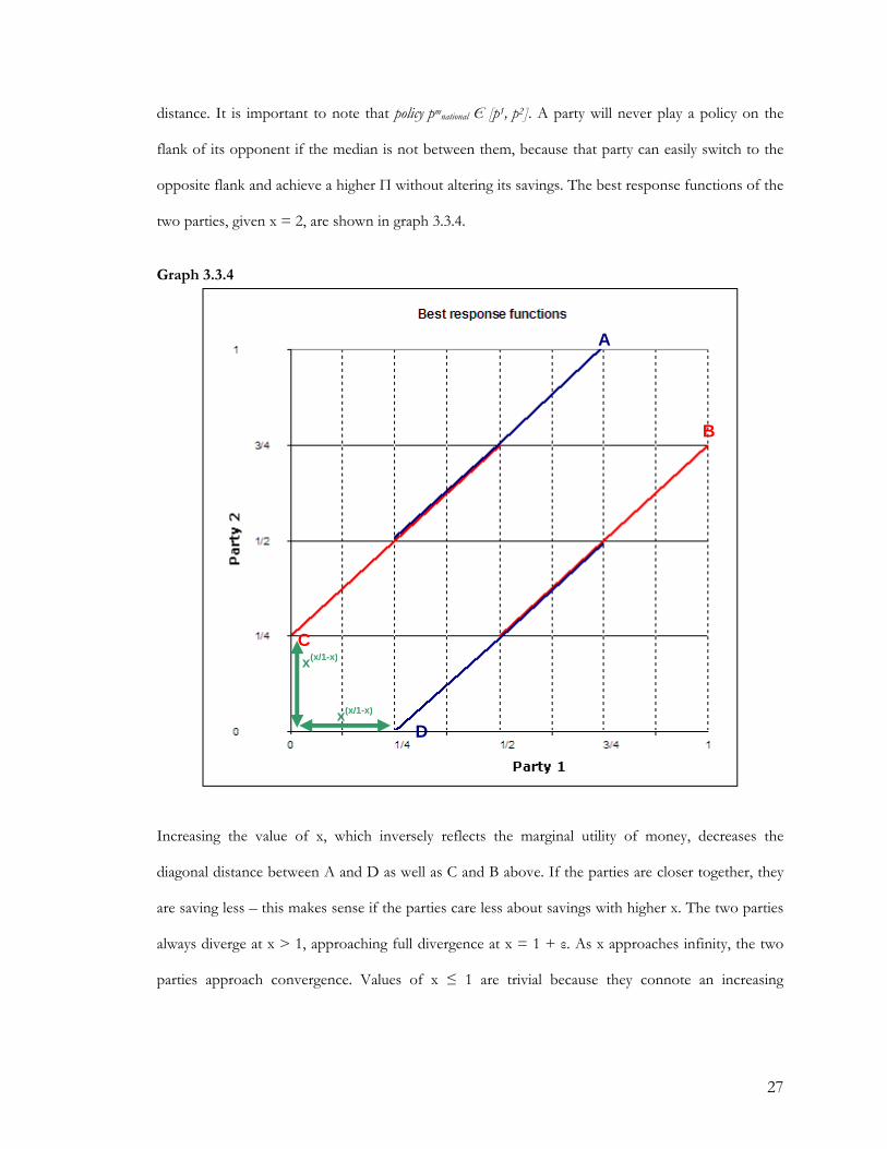
opposite flank and achieve a higher Π without altering its savings. The best response functions of the

two parties, given x = 2, are shown in graph 3.3.4.

Graph 3.3.4

A

B

C x(x/1-x)

x(x/1-x) D

Increasing the value of x, which inversely reflects the marginal utility of money, decreases the

diagonal distance between A and D as well as C and B above. If the parties are closer together, they

are saving less – this makes sense if the parties care less about savings with higher x. The two parties

always diverge at x > 1, approaching full divergence at x = 1 + ε. As x approaches infinity, the two

parties approach convergence. Values of x ≤ 1 are trivial because they connote an increasing

27

marginal utility of money, and lead to a distance between parties that is either undefined or negative

and large.

This section has shown that if parties care about savings, they will not want to spend their

entire budget. Given a utility function that rewards parties for not financing all contestable elections,

divergence becomes possible. Party i will always wish to be x(x/(1– x)) away from party j, as long as the

national median policy is between them. The next section explores the effect of a budget restriction

on this conclusion.

3.4 Two Party Model: Restricted Budget, Utility from Payoffs and Money

In section 3.2, it was established that restraining the budget leads to two results: initial

aggressive budgeting, followed by convergence to the national median and indifference regarding where

the budget is placed. Aggressive budgeting implies that party i places it’s budget Bi, or the largest part

of Bi, facing the other party’s position pj. For simplicity, it will be assumed that parties pursue

aggressive budgeting no matter what, and do not change to a different budgeting choice if they are

indifferent between two options.

The last section also showed that a party will want to position itself such that x(x/(1– x)) is

saved. This is so because the slope of V(Si) equals the negative slope of Πi at that point, and is the

maximum of the utility function. Thus if a party finances all the elections up to x(x/(1– x)) away from

the competing platform, the next election’s marginal payoff from votes is higher than the marginal

utility from savings. Conversely, the marginal gain in savings provides more utility than the marginal

payoff from votes for all elections within the distance x(x/(1– x)). For x = 2, x(x/(1– x)) equals 1/4. A party

will always want to save 1/4 and spend the rest on financing elections, no more and no less. When

the budget is unrestricted, or equal to 1/2, the parties push apart in order to limit the overlap of

contestable elections to 1/4. In the case of a restricted budget, the situation is somewhat different. I

first examine the situation with a budget constraint of B = 1/8. Next, I look at B = 2/8 and then B =

28

3/8. It is again assumed that c = 1/2; this provides cleaner results because c is not “too large”,

requiring the use of min/max functions.

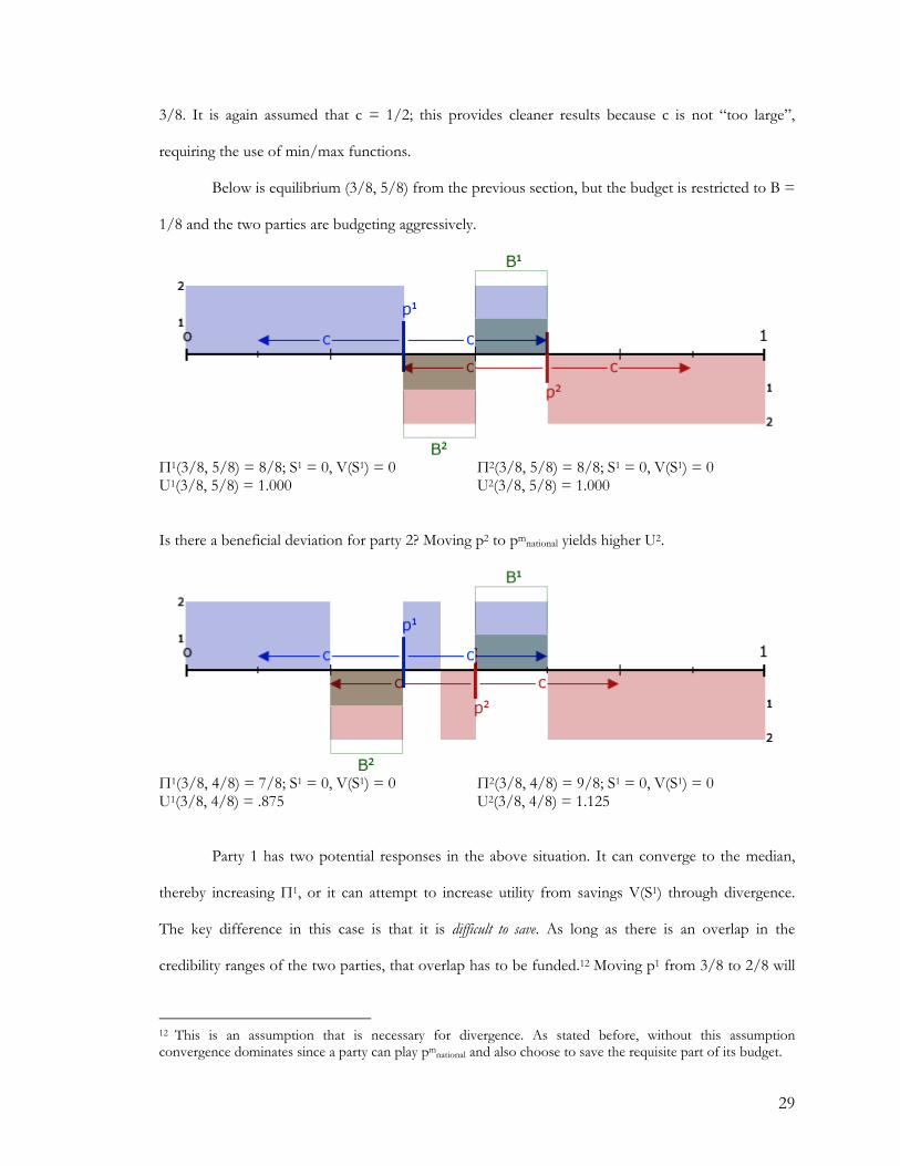
Below is equilibrium (3/8, 5/8) from the previous section, but the budget is restricted to B =

1/8 and the two parties are budgeting aggressively.

Π1(3/8, 5/8) = 8/8; S1 = 0, V(S1) = 0 Π2(3/8, 5/8) = 8/8; S1 = 0, V(S1) = 0 U1(3/8, 5/8) = 1.000 U2(3/8, 5/8) = 1.000

Is there a beneficial deviation for party 2? Moving p2 to pmnational yields higher U2.

Π1(3/8, 4/8) = 7/8; S1 = 0, V(S1) = 0 Π2(3/8, 4/8) = 9/8; S1 = 0, V(S1) = 0 U1(3/8, 4/8) = .875 U2(3/8, 4/8) = 1.125

Party 1 has two potential responses in the above situation. It can converge to the median,

thereby increasing Π1, or it can attempt to increase utility from savings V(S1) through divergence.

The key difference in this case is that it is difficult to save. As long as there is an overlap in the

credibility ranges of the two parties, that overlap has to be funded.12 Moving p1 from 3/8 to 2/8 will

12 This is an assumption that is necessary for divergence. As stated before, without this assumption convergence dominates since a party can play pmnational and also choose to save the requisite part of its budget.

29

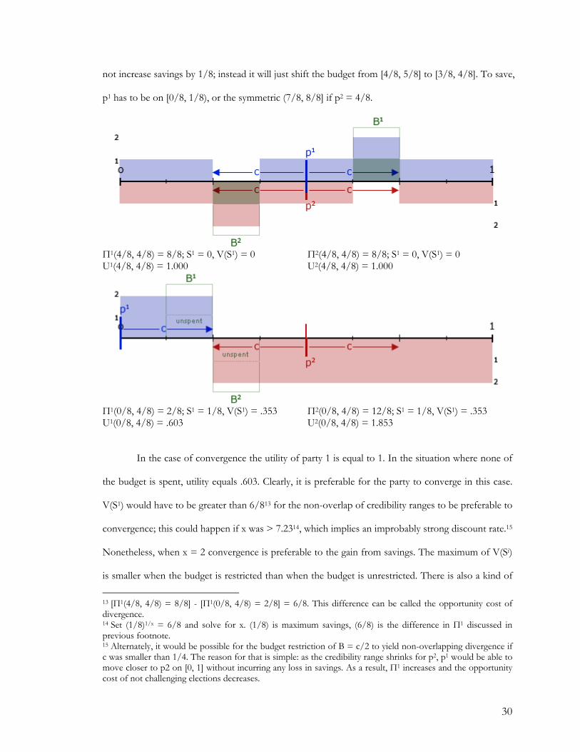
not increase savings by 1/8; instead it will just shift the budget from [4/8, 5/8] to [3/8, 4/8]. To save,

p1 has to be on [0/8, 1/8), or the symmetric (7/8, 8/8] if p2 = 4/8.

Π1(4/8, 4/8) = 8/8; S1 = 0, V(S1) = 0 Π2(4/8, 4/8) = 8/8; S1 = 0, V(S1) = 0 U1(4/8, 4/8) = 1.000 U2(4/8, 4/8) = 1.000

Π1(0/8, 4/8) = 2/8; S1 = 1/8, V(S1) = .353 Π2(0/8, 4/8) = 12/8; S1 = 1/8, V(S1) = .353 U1(0/8, 4/8) = .603 U2(0/8, 4/8) = 1.853

In the case of convergence the utility of party 1 is equal to 1. In the situation where none of

the budget is spent, utility equals .603. Clearly, it is preferable for the party to converge in this case.

V(S1) would have to be greater than 6/813 for the non-overlap of credibility ranges to be preferable to

convergence; this could happen if x was > 7.2314, which implies an improbably strong discount rate.15

Nonetheless, when x = 2 convergence is preferable to the gain from savings. The maximum of V(Si)

is smaller when the budget is restricted than when the budget is unrestricted. There is also a kind of

13 [Π1(4/8, 4/8) = 8/8] - [Π1(0/8, 4/8) = 2/8] = 6/8. This difference can be called the opportunity cost of divergence. 14 Set (1/8)1/x = 6/8 and solve for x. (1/8) is maximum savings, (6/8) is the difference in Π1 discussed in previous footnote. 15 Alternately, it would be possible for the budget restriction of B = c/2 to yield non-overlapping divergence if c was smaller than 1/4. The reason for that is simple: as the credibility range shrinks for p2, p1 would be able to move closer to p2 on [0, 1] without incurring any loss in savings. As a result, Π1 increases and the opportunity cost of not challenging elections decreases.

30

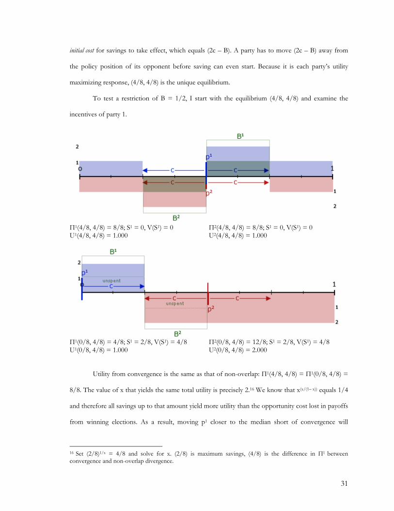
initial cost for savings to take effect, which equals (2c – B). A party has to move (2c – B) away from

the policy position of its opponent before saving can even start. Because it is each party’s utility

maximizing response, (4/8, 4/8) is the unique equilibrium.

To test a restriction of B = 1/2, I start with the equilibrium (4/8, 4/8) and examine the

incentives of party 1.

Π1(4/8, 4/8) = 8/8; S1 = 0, V(S1) = 0 Π2(4/8, 4/8) = 8/8; S1 = 0, V(S1) = 0 U1(4/8, 4/8) = 1.000 U2(4/8, 4/8) = 1.000

Π1(0/8, 4/8) = 4/8; S1 = 2/8, V(S1) = 4/8 Π2(0/8, 4/8) = 12/8; S1 = 2/8, V(S1) = 4/8 U1(0/8, 4/8) = 1.000 U2(0/8, 4/8) = 2.000

Utility from convergence is the same as that of non-overlap: Π1(4/8, 4/8) = Π1(0/8, 4/8) =

8/8. The value of x that yields the same total utility is precisely 2.16 We know that x(x/(1– x)) equals 1/4

and therefore all savings up to that amount yield more utility than the opportunity cost lost in payoffs

from winning elections. As a result, moving p1 closer to the median short of convergence will

16 Set (2/8)1/x = 4/8 and solve for x. (2/8) is maximum savings, (4/8) is the difference in Π1 between convergence and non-overlap divergence.

31

decrease total utility. If party 2 initially plays p2 = 4/8, the possible equilibria are (0/8, 4/8), (4/8, 4/8)

and (8/8, 4/8). Otherwise, the parties will keep a distance of 1/2 to achieve the maximum payoff

from savings, yielding a set of equilibria similar to that of section 3.3. Convergence should not occur

at policy pairs other than (pmnational, pmnational) – in policy pair (p1, p1) party 2 can always move to the

national median and increase utility since U(p1, p1) < U(p1, pmnational).

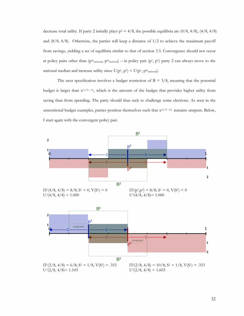
The next specification involves a budget restriction of B = 3/8, meaning that the potential

budget is larger than x(x/(1– x)), which is the amount of the budget that provides higher utility from

saving than from spending. The party should thus seek to challenge some elections. As seen in the

unrestricted budget examples, parties position themselves such that x(x/(1– x)) remains unspent. Below,

I start again with the convergent policy pair.

Π1(4/8, 4/8) = 8/8; S1 = 0, V(S1) = 0 Π2(p1,p2) = 8/8; S1 = 0, V(S1) = 0 U1(4/8, 4/8) = 1.000 U2(4/8, 4/8)= 1.000

Π1(2/8, 4/8) = 6/8; S1 = 1/8, V(S1) = .353 Π2(2/8, 4/8) = 10/8; S1 = 1/8, V(S1) = .353 U1(2/8, 4/8)= 1.103 U2(2/8, 4/8) = 1.603

32

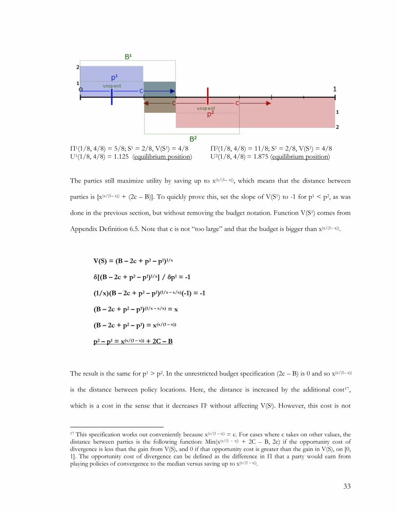
Π1(1/8, 4/8) = 5/8; S1 = 2/8, V(S1) = 4/8 Π2(1/8, 4/8) = 11/8; S1 = 2/8, V(S1) = 4/8 U1(1/8, 4/8) = 1.125 (equilibrium position) U2(1/8, 4/8) = 1.875 (equilibrium position)

The parties still maximize utility by saving up to x(x/(1– x)), which means that the distance between

parties is [x(x/(1– x)) + (2c – B)]. To quickly prove this, set the slope of V(S1) to -1 for p1 < p2, as was

done in the previous section, but without removing the budget notation. Function V(S1) comes from

Appendix Definition 6.5. Note that c is not “too large” and that the budget is bigger than x(x/(1– x)).

V(S) = (B – 2c + p2 – p1)1/x

δ[(B – 2c + p2 – p1)1/x] / δp1 = -1

(1/x)(B – 2c + p2 – p1)(1/x – x/x)(-1) = -1

(B – 2c + p2 – p1)(1/x – x/x) = x

(B – 2c + p2 – p1) = x(x/(1 – x))

p2 – p1 = x(x/(1 – x)) + 2C – B

The result is the same for p1 > p2. In the unrestricted budget specification (2c – B) is 0 and so x(x/(1– x))

is the distance between policy locations. Here, the distance is increased by the additional cost17,

which is a cost in the sense that it decreases Πi without affecting V(Si). However, this cost is not

17 This specification works out conveniently because x(x/(1 – x)) = c. For cases where c takes on other values, the distance between parties is the following function: Min(x(x/(1 – x)) + 2C – B, 2c) if the opportunity cost of divergence is less than the gain from V(S), and 0 if that opportunity cost is greater than the gain in V(S), on [0, 1]. The opportunity cost of divergence can be defined as the difference in Π that a party would earn from playing policies of convergence to the median versus saving up to x(x/(1 – x)).

33

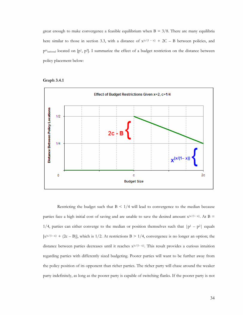
great enough to make convergence a feasible equilibrium when B = 3/8. There are many equilibria

here similar to those in section 3.3, with a distance of x(x/(1 – x)) + 2C – B between policies, and

pmnational located on [p1, p2]. I summarize the effect of a budget restriction on the distance between

policy placement below:

Graph 3.4.1

Restricting the budget such that B < 1/4 will lead to convergence to the median because

parties face a high initial cost of saving and are unable to save the desired amount x(x/(1– x)). At B =

1/4, parties can either converge to the median or position themselves such that |p1 – p2| equals

[x(x/(1– x)) + (2c – B)], which is 1/2. At restrictions B > 1/4, convergence is no longer an option; the

distance between parties decreases until it reaches x(x/(1– x)). This result provides a curious intuition

regarding parties with differently sized budgeting. Poorer parties will want to be further away from

the policy position of its opponent than richer parties. The richer party will chase around the weaker

party indefinitely, as long as the poorer party is capable of switching flanks. If the poorer party is not

34

allowed to switch flanks, it is likely that the wealthier party will back it into a corner and capture a

much larger payoff.

3.5 Three Party Model: Unrestricted Budget, Utility from Payoffs and Money

In this section, a third party considers entering the national electoral competition with an

unrestricted budget and the amended utility function. I focus on the incentives of the new party,

rather than looking for a three party equilibrium, because I am interested specifically in the issue of

entry. The definitions are as follows:

Ui = U [Πi(pi, pj, pk)] = Πi(pi, pj, pk) + V(Si)

Πi(pi, pj, pk) = (payoff of local district)(district portion)

Unchallenged election payoff: victory = 2, loss = 0

Challenged election payoff = [2/(amount of parties challenging district)]

Si = (B – Ci(pi, pj, pk)); B = 2c

Ci(pi, pj, pk) = (cost of local district = 1)(district portion)

V(Si) = (Si)1/x; x = 2

There are multiple initial two party equilibria such that the parties are playing policies 1/4 apart. First,

I examine policy set (4/8, 2/8, p3), fixing the location of the first two parties. Party 2 plays the most

“extreme”18 policy possible, allowing party 3 to achieve the highest utility, as will be shown. The

example explored afterwards focuses on (5/8, 3/8, p3), which provides party 3 with the lowest utility.

These two examples define the range of available U3 given different starting equilibria.

18 Since p1 and p2 will never both be to the same side of the median, p1 = 1/2 creates the most extreme asymmetry.

35

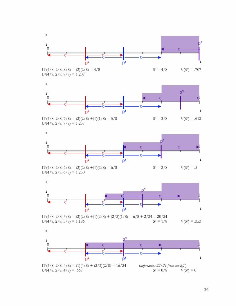
Π3(4/8, 2/8, 8/8) = (2)(2/8) = 4/8 S3 = 4/8 V(S3) = .707 U3(4/8, 2/8, 8/8) = 1.207

Π3(4/8, 2/8, 7/8) = (2)(2/8) +(1)(1/8) = 5/8 S3 = 3/8 V(S3) = .612 U3(4/8, 2/8, 7/8) = 1.237

Π3(4/8, 2/8, 6/8) = (2)(2/8) +(1)(2/8) = 6/8 S3 = 2/8 V(S3) = .5 U3(4/8, 2/8, 6/8) = 1.250

Π3(4/8, 2/8, 5/8) = (2)(2/8) +(1)(2/8) + (2/3)(1/8) = 6/8 + 2/24 = 20/24 U3(4/8, 2/8, 5/8) = 1.186 S3 = 1/8 V(S3) = .353

Π3(4/8, 2/8, 4/8) = (1)(4/8) + (2/3)(2/8) = 16/24 (approaches 22/24 from the left ) U3(4/8, 2/8, 4/8) = .667 S3 = 0/8 V(S3) = 0

36

Policies p3 < p1 are not explored because their payoffs are significantly lower than those

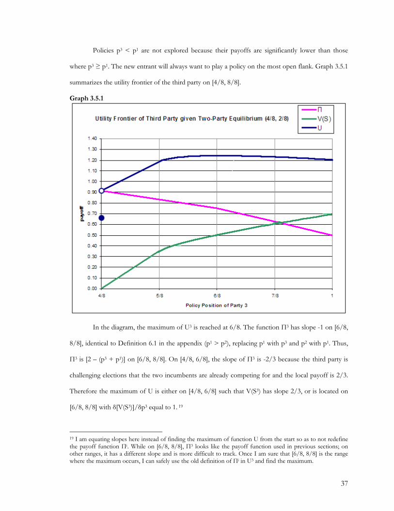
where p3 ≥ p1. The new entrant will always want to play a policy on the most open flank. Graph 3.5.1

summarizes the utility frontier of the third party on [4/8, 8/8].

Graph 3.5.1

In the diagram, the maximum of U3 is reached at 6/8. The function Π3 has slope -1 on [6/8,

8/8], identical to Definition 6.1 in the appendix (p1 > p2), replacing p1 with p3 and p2 with p1. Thus,

Π3 is [2 – (p3 + p1)] on [6/8, 8/8]. On [4/8, 6/8], the slope of Π3 is -2/3 because the third party is

challenging elections that the two incumbents are already competing for and the local payoff is 2/3.

Therefore the maximum of U is either on [4/8, 6/8] such that V(S3) has slope 2/3, or is located on

[6/8, 8/8] with δ[V(S3)]/δp3 equal to 1. 19

19 I am equating slopes here instead of finding the maximum of function U from the start so as to not redefine the payoff function Πi. While on [6/8, 8/8], Π3 looks like the payoff function used in previous sections; on other ranges, it has a different slope and is more difficult to track. Once I am sure that [6/8, 8/8] is the range where the maximum occurs, I can safely use the old definition of Πi in U3 and find the maximum.

37

The slope of V3 equals 2/3 at p3 = 17/16, found by setting the derivate of V3 with respect to

p3 equal to 2/3. This is outside the policy space. The other option for the maximum is on [6/8, 8/8],

where Π3 is regularly defined.

Π3(4/8, 2/8, p3) = 16/8 – (4/8 + p3); V(S3) = (p3 – 4/8)1/2

U3 = 12/8 – p3 + (p3 – 4/8)1/2

δ[12/8 – p3 + (p3 – 4/8)1/2]/δp3 = 0 0 + -1 + 1/2(p3 – 4/8)-1/2 = 0

2 = (p3 – 4/8)-1/2 4 = 1/(p3 – 4/8) 2/8 = p3 – 4/8 p3 = 6/8

The maximum utility is at policy position 6/8, which is precisely 1/4 away from 4/8, the position of

party 1. It is anticipated that the new entrant will play a policy with distance x(x/(1– x)) from the party

closest to the median. The highest utility available to party 3 is at (4/8, 2/8, 6/8), where U3(Π3,

V(S3))= 12/8 – 6/8 + (6/8 – 4/8)1/2 = 10/8.

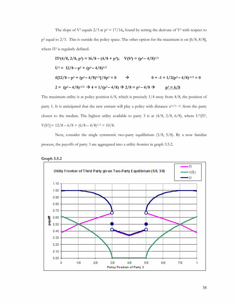
Next, consider the single symmetric two-party equilibrium (3/8, 5/8). By a now familiar

process, the payoffs of party 3 are aggregated into a utility frontier in graph 3.5.2.

Graph 3.5.2

38

An important caveat is that party 3 would never play policy p2 ≥ p3 ≥ p1 because the payoffs

are significantly lower in that range. The largest benefit is gained by entering from a side and

capturing the flank: the payoffs are symmetric on either side. To find the preferred position for the

third party, I focus on [4/8, 8/8] to be consistent with the previous example.

Π3(5/8, 3/8, p3) = 16/8 – (5/8 + p3); V(S3) = (p3 – 5/8)1/2

U3 = 11/8 – p3 + (p3 – 5/8)1/2

δ [11/8 – p3 + (p3 – 5/8)1/2]/δp3 = 0 0 + -1 + 1/2(p3 – 5/8)-1/2 = 0

2 = (p3 – 5/8)-1/2 4 = 1/( p3 – 5/8) 2/8 = p3 – 5/8 p3 = 7/8

The policy set (5/8, 3/8, 7/8) and the symmetric (5/8, 3/8, 1/8) provide the third party with the

maximum utility. It again locates 1/4 away from the party closest to the national median. Below, I

generalize the incentives of party 3 given the symmetric equilibrium of the incumbents.

If p3 > p1

Π3(p1, p2, p3) = 2 – (p1 + p3)

V(S3) = ((B – 2c) + p3 – p1)1/x

U1 = 2 – (p3 + p1) + (p3 – p1)1/x

δ[2 – p1 – p3 + (p3 – p1)1/x] / δp3 = 0

(0) – 1 + (1/x)(p3 – p1)(1/x – x/x)(1) = 0

1 = (1/x)(p3 – p1)(1/x – x/x)

x = (p3 – p1)((1 –x)/x)

x(x/(1 – x)) = (p3 – p1)

x(x/(1 – x)) + p1 = p3

p3 = p1 + x(x/(1 – x))

If p3 < p2

Π3(p1, p2, p3) = p2 + p3

V(S3) = ((B – 2c) + p2 – p3)1/x

U1 = p3 + p2 + (p2 – p3)1/x

δ[ p3 + p2 + (p2 – p3)1/x ] / δp3 = 0

1 + 0 + (1/x)(p2 – p3)(1/x – x/x)(-1) = 0

1 = (1/x)(p2 – p3)(1/x – x/x)

x = (p2 – p3)((1 –x)/x)

x(x/(1 – x)) = (p2 – p3)

p3 + x(x/(1 – x)) = p2

p3 = p2 – x(x/(1– x))

39

Party 3 will always play p3 such that Min[|p3 – p2|, |p3 – p1|] = x(x/(1 – x)). It will not position

itself between the two incumbents. At (5/8, 3/8, 7/8), the third party achieves a maximum U3 =

11/8 – 7/8 + (7/8 – 5/8)1/2 = 8/8. This is the minimum utility that parties 1 and 2 can force on the

third party. The full range of U3 is [8/8, 10/8], where U3 depends on the equilibrium of the first two

players.

The possibility of entry should impact the behavior of the original two parties. A full

exploration of that dynamic is beyond the scope of this paper20, but here is the intuition behind the

problem. A third party has a significant negative effect on the utility of the party whose flank it

consumes; the new competition drastically reduces the challenged incumbent’s savings. If possible,

the challenged incumbent will move to a location where it can again achieve a savings of x(x/(1 – x)).

This is likely to be prevented by the party on the other flank, which will react by moving towards the

extreme, keeping a fixed distance away from its opponent. Thus the central party has difficulty

achieving a high utility. Notably, cooperatively merging with the other incumbent may be a good idea

because competition is reduced and savings is again possible. If a merger happens, the new

“incumbent” moves towards the new entrant until savings equals x(x/(1 – x)).

3.6 Three Party Model: Restricted Budget, Utility from Payoffs and Money

In reality, political parties come in different sizes. They certainly have different national

budgets. Despite some variation, it can be said that the budgets of Republicans and Democrats are

unrestricted in this model. Both parties are capable of raising a tremendous amount of money,

funding contestable elections across the country up to the necessary limit. As in section 3.5, the two

incumbent parties have a budget B = 2c. The third party, however, is an underdog. It is likely to have

a much sharper budget constraint, because raising money for a political start-up is difficult. Even

“established” third parties, like the Libertarians or the Green party, have tiny budgets compared to

20 In thinking about Duverger’s Law, I am trying to show that entry is prohibitively difficult, rather than the full effects of entry on the incumbents.

40

that of the two incumbents. Furthermore, they challenge very few elections, instead serving a

symbolic function of signaling to the larger parties preferences of the American populace.

In section 3.5, an entrant is very dangerous to parties 1 and 2, capable of capturing an entire

flank and severely crippling the incumbent caught in the middle. This result is based on the

assumption that the new entrant instantaneously assumes national-party stature, with B = 2c, c = 1/2.

However, it is easy to imagine that budget B3 is in fact significantly lower, by a very high magnitude

in the United States21. Restricting B3 to c/2 simulates the deep asymmetry in available financing

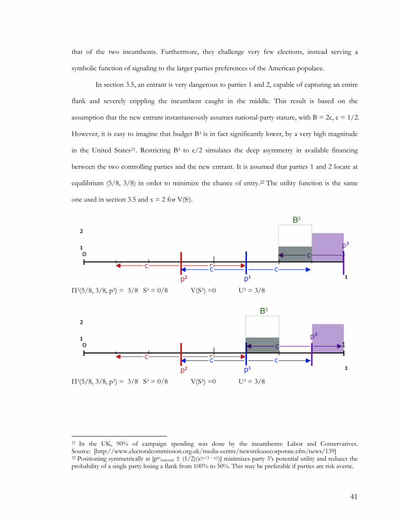
between the two controlling parties and the new entrant. It is assumed that parties 1 and 2 locate at

equilibrium (5/8, 3/8) in order to minimize the chance of entry.22 The utility function is the same

one used in section 3.5 and x = 2 for V(Si).

Π3(5/8, 3/8, p3) = 3/8 S3 = 0/8 V(S3) =0 U3 = 3/8

Π3(5/8, 3/8, p3) = 3/8 S3 = 0/8 V(S3) =0 U3 = 3/8

21 In the UK, 90% of campaign spending was done by the incumbents: Labor and Conservatives. Source: [http://www.electoralcommission.org.uk/media-centre/newsreleasecorporate.cfm/news/139] 22 Positioning symmetrically at [pmnational ± (1/2)(x(x/(1 – x)))] minimizes party 3’s potential utility and reduces the probability of a single party losing a flank from 100% to 50%. This may be preferable if parties are risk averse.

41

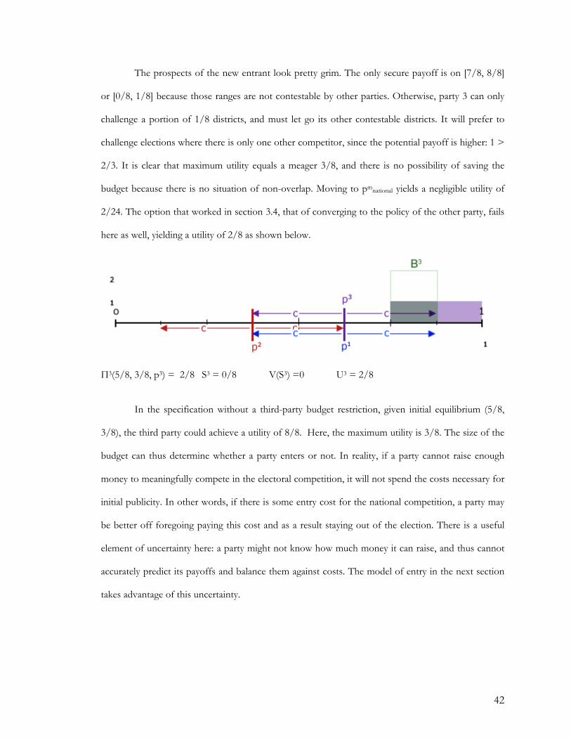
The prospects of the new entrant look pretty grim. The only secure payoff is on [7/8, 8/8]

or [0/8, 1/8] because those ranges are not contestable by other parties. Otherwise, party 3 can only

challenge a portion of 1/8 districts, and must let go its other contestable districts. It will prefer to

challenge elections where there is only one other competitor, since the potential payoff is higher: 1 >

2/3. It is clear that maximum utility equals a meager 3/8, and there is no possibility of saving the

budget because there is no situation of non-overlap. Moving to pmnational yields a negligible utility of

2/24. The option that worked in section 3.4, that of converging to the policy of the other party, fails

here as well, yielding a utility of 2/8 as shown below.

Π3(5/8, 3/8, p3) = 2/8 S3 = 0/8 V(S3) =0 U3 = 2/8

In the specification without a third-party budget restriction, given initial equilibrium (5/8,

3/8), the third party could achieve a utility of 8/8. Here, the maximum utility is 3/8. The size of the

budget can thus determine whether a party enters or not. In reality, if a party cannot raise enough

money to meaningfully compete in the electoral competition, it will not spend the costs necessary for

initial publicity. In other words, if there is some entry cost for the national competition, a party may

be better off foregoing paying this cost and as a result staying out of the election. There is a useful

element of uncertainty here: a party might not know how much money it can raise, and thus cannot

accurately predict its payoffs and balance them against costs. The model of entry in the next section

takes advantage of this uncertainty.

42

4 – Entry

The new entrant faces a lump-sum entry cost α. This cost is the price paid for national

advertising and other marketing. It establishes the credibility range by informing relevant districts

about the new entrant’s potential candidates: the cost of informing each district is 1, and the total

cost is (local cost)(district portion informed). For consistency, that district portion is the incumbent

credibility range 2c. 23 A new party will enter if expected utility is greater than utility derived from

saving the lump sum. Function V is used here again: the entry cost can be “saved” and the same

utility derived as if the party were saving its budget. The third party, instead of spending α on entry,

could use that money to finance political seminars or impact policy through lobbying. To summarize:

α is the entry cost for the national electoral competition, α = 2c

V(α) = (α)1/x, x = 2

If V(α) ≥ Uk [Πk, V(Sk)], the party does not enter the electoral competition

If V(α) < Uk [Πk, V(Sk)], the party enters the electoral competition

Pk(V(α) < Uk [Πk, V(Sk)]) is the probability with which the party enters the electoral competition

The new entrant does not know how much money it will be able to raise: budget B is a random

variable on [0, 2c] with mean c. Thus the expected budget of the third party is E(B) = c. The current

utility threshold for entry, given 2c = 1/2, is V(α = 1/2) = .707. To calculate the expected utility of

the new entrant, restrict the budget to 1/4 and consider the policy triple (5/8, 3/8, p3). Party 3

maximizes utility by playing either p3 = 1/8 or p3 = 7/8, achieving U3 = .500.24 As a result, U3 < V(α)

and the probability of entry is 0. If the initial incumbent equilibrium is symmetric around the national

23 This paper does not explore credibility ranges of different sizes, although arguably a new party will have a much smaller credibility range. Changing the credibility range assumption is certainly an interesting direction to explore, and is likely to allow more fringe parties to enter due to lowered entry costs. However, a smaller credibility range acts also as a constraint on the maximum, or “unrestricted” budget, while the marginal utility of money is likely to stay the same. Thus parties could want to save 1/4 while having a credibility range of 1/8. The author hypothesizes that in a country like India, which has many different parties nationally, credibility ranges are relatively small throughout. 24 The assumption of symmetric equilibria is meant to reflect risk-averse incumbents.

43

median, which should happen if parties 1 and 2 are moderately risk averse, the third party will not

enter electoral competition. Entry is possible if the incumbents are located closer to (6/8, 4/8, p3)

because the third party can achieve a U3 = .750 in that situation. However, it is unlikely that the

incumbent parties would open up their flanks in this manner, because losing one’s flank reduces

payoffs catastrophically.

This paper ends on the model of entry because entry is key to the main question I am

addressing – why does Duverger’s Law hold? United States electoral competitions have always been

dominated by the two party system. In the entire history of the country, an incumbent party only

once lost its position to a challenger: the Whigs disintegrated allowing for the rise of the Republicans.

This two party equilibrium holds because entry is almost impossible. What new party can raise

enough money for both the entry cost and the unrestricted budget? Thus third parties are almost

non-existent on the national scale.

44

5 – Conclusion

On some level, the model raises as many questions as it answers. What are the effects of

changing the size of the credibility range? What if parties have different marginal utilities of savings?

How exactly do incumbents respond to entry, and should there be a model of exit? Do parties have to

finance contestable elections, or can they simply position themselves anywhere and save the budget

as desired? These are interesting questions to explore and limitations of this thesis. However, the

assumptions in this paper are meant to reflect electoral competition in the United States and similar

countries. In this situation, parties credibly compete over a large portion of the populace. Democrats

and Republicans are seen as capable of representing voters in the majority of states – in 2004, there

was only one Independent in the Senate. Additionally, campaign financing is not particularly

restrictive and the incumbent parties have little trouble raising tremendous amounts of money, while

new entrants face great uncertainty in their fundraising.

The logic of this model provides a number of separate useful results. First, despite electoral

competition taking place on a continuum of districts, parties still converge if they are motivated only

by winning elections. If parties care about savings and have a diminishing marginal utility of money,

they will move apart their policies in order to save a certain amount of their budget. This amount

depends essentially on greed. A third party entrant with similar preferences will want to also locate a

distance away from the incumbents, taking the most advantageous flank. This entry is very damaging

to the party caught in the middle. Budget restrictions, which reflect either legislation that limits

fundraising or simply a lesser ability to acquire money, have complicated effects. Despite occasionally

leading to convergence, restrictions primarily increase the distance between party policies by creating

an additional opportunity cost to savings in terms of election victories. A third party entrant with a

restricted budget faces grim circumstances – a very low utility. Using a simple, although somewhat

arbitrary, model of entry I show that uncertainty regarding an entrant’s potential budget translates

into a low expected utility, and therefore precludes entry. The two-party equilibrium remains

unchallenged and Duverger’s Law holds.

45

6 – Appendix

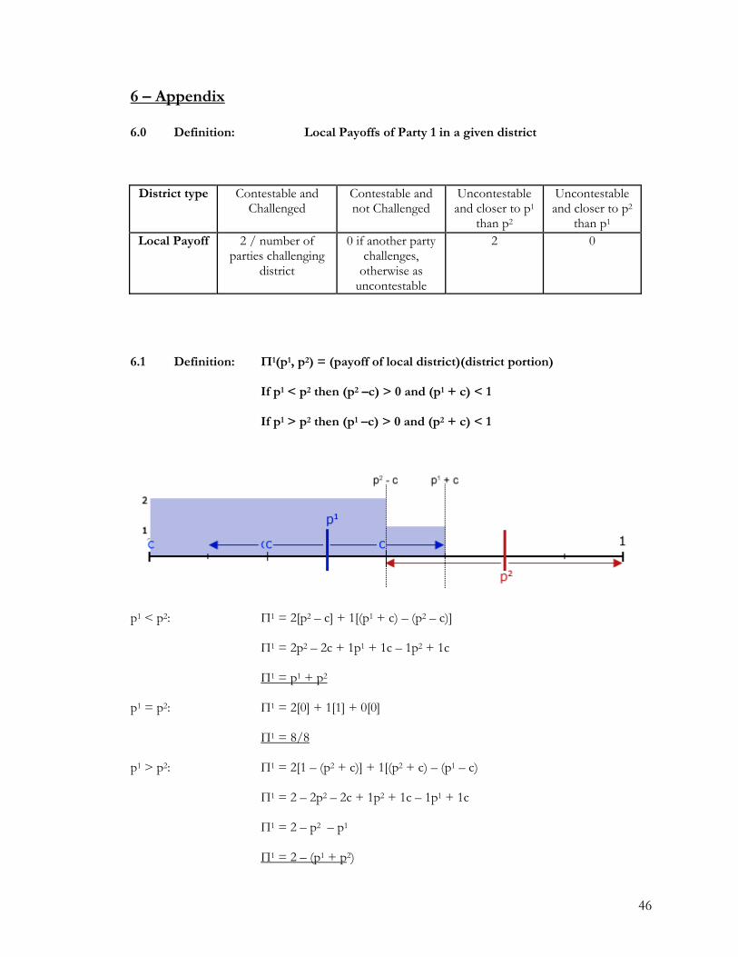
6.0 Definition: Local Payoffs of Party 1 in a given district

District type Contestable and Challenged

Contestable and not Challenged

Uncontestable and closer to p1

than p2

Uncontestable and closer to p2

than p1 Local Payoff 2 / number of

parties challenging district

0 if another party challenges,

otherwise as uncontestable

2 0

6.1 Definition: Π1(p1, p2) = (payoff of local district)(district portion)

If p1 < p2 then (p2 –c) > 0 and (p1 + c) < 1

If p1 > p2 then (p1 –c) > 0 and (p2 + c) < 1

p1 < p2: Π1 = 2[p2 – c] + 1[(p1 + c) – (p2 – c)]

Π1 = 2p2 – 2c + 1p1 + 1c – 1p2 + 1c

Π1 = p1 + p2

p1 = p2: Π1 = 2[0] + 1[1] + 0[0]

Π1 = 8/8

p1 > p2: Π1 = 2[1 – (p2 + c)] + 1[(p2 + c) – (p1 – c)

Π1 = 2 – 2p2 – 2c + 1p2 + 1c – 1p1 + 1c

Π1 = 2 – p2 – p1

Π1 = 2 – (p1 + p2)

46

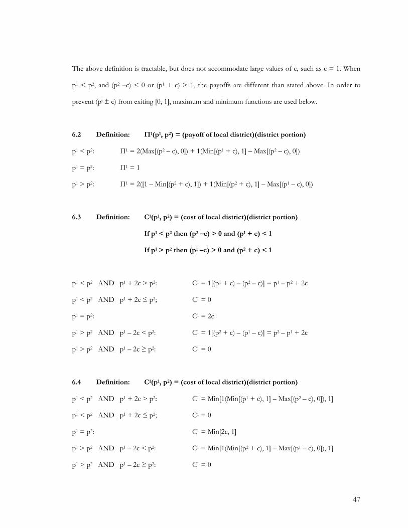
The above definition is tractable, but does not accommodate large values of c, such as c = 1. When

p1 < p2, and (p2 –c) < 0 or (p1 + c) > 1, the payoffs are different than stated above. In order to

prevent (pi ± c) from exiting [0, 1], maximum and minimum functions are used below.

6.2 Definition: Π1(p1, p2) = (payoff of local district)(district portion)

p1 < p2: Π1 = 2(Max[(p2 – c), 0]) + 1(Min[(p1 + c), 1] – Max[(p2 – c), 0])

p1 = p2: Π1 = 1

p1 > p2: Π1 = 2([1 – Min[(p2 + c), 1]) + 1(Min[(p2 + c), 1] – Max[(p1 – c), 0])

6.3 Definition: C1(p1, p2) = (cost of local district)(district portion)

If p1 < p2 then (p2 –c) > 0 and (p1 + c) < 1

If p1 > p2 then (p1 –c) > 0 and (p2 + c) < 1

p1 < p2 AND p1 + 2c > p2: C1 = 1[(p1 + c) – (p2 – c)] = p1 – p2 + 2c

p1 < p2 AND p1 + 2c ≤ p2; C1 = 0

p1 = p2: C1 = 2c

p1 > p2 AND p1 – 2c < p2: C1 = 1[(p2 + c) – (p1 – c)] = p2 – p1 + 2c

p1 > p2 AND p1 – 2c ≥ p2: C1 = 0

6.4 Definition: C1(p1, p2) = (cost of local district)(district portion)

p1 < p2 AND p1 + 2c > p2: C1 = Min[1(Min[(p1 + c), 1] – Max[(p2 – c), 0]), 1]

p1 < p2 AND p1 + 2c ≤ p2; C1 = 0

p1 = p2: C1 = Min[2c, 1]

p1 > p2 AND p1 – 2c < p2: C1 = Min[1(Min[(p2 + c), 1] – Max[(p1 – c), 0]), 1]

p1 > p2 AND p1 – 2c ≥ p2: C1 = 0

47

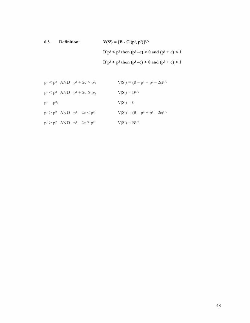
6.5 Definition: V(S1) = [B - C1(p1, p2)]1/x

If p1 < p2 then (p2 –c) > 0 and (p1 + c) < 1

If p1 > p2 then (p1 –c) > 0 and (p2 + c) < 1

p1 < p2 AND p1 + 2c > p2: V(S1) = (B – p1 + p2 – 2c)1/2

p1 < p2 AND p1 + 2c ≤ p2; V(S1) = B1/2

p1 = p2: V(S1) = 0

p1 > p2 AND p1 – 2c < p2: V(S1) = (B – p2 + p1 – 2c)1/2

p1 > p2 AND p1 – 2c ≥ p2: V(S1) = B1/2

48

7 – Bibliography

Arrow, Kenneth and Sen. Amartya. 2002. Handbook of Social Choice and Welfare. Amsterdam: Elsevier Science B. V. Besley, T., and S. Coate. 1997. “An economic model of representative democracy.” Quarterly Journal of Economics 112:85-114. Callander, S. 1999. “Electoral Competition with Entry.” California Institute of Technology, Division of the Humanities and Social Sciences, Working Papers: 1083. Caplan, B. 2001. "When Is Two Better Than One? How Federalism Mitigates and Intensifies Imperfect Political Competition." Journal of Public Economics 80(1): 99-119. Chhibber, P., and K. Kollman. 1998. “Party Aggregation and the Number of Parties in India and the United States.” The American Political Science Review 92(2): 329-342 Coughlin, P., and S. Nitzan .1981. “Electoral outcomes with probabilistic voting and Nash social welfare maxima.” Journal of Public Economics 15:113-121. Cox, G. W. 1997. Making votes count: Strategic coordination in the world's electoral systems. Cambridge; New York and Melbourne, Cambridge University Press. Downs, Anthony. 1957. An Economic Theory of Democracy. New York: Harper and Row. Duggan, J. and M. Fey. 2005. "Electoral Competition with Policy-Motivated Candidates." Games and Economic Behavior 51(2): 490-522. Duverger, M. 1963. Political Parties: their organization and activity in the modern state, North, B, and North R., tr. New York: Wiley, Science Ed. Eyster, E. and T. Kittsteiner. 2004. “Party Platforms in Electoral Competition with many constituencies.” University of Bonn, Bonn Econ Discussion Papers. Federsen, Timothy, I. Sened and S. G. Wright. 1990. “rational Voting and Candidate Entry under Plurality Rule.” American Journal of Political Science 34:1005-1016. Goeree, J. K. and C. A. Holt. 2005. "An Explanation of Anomalous Behavior in Models of Political Participation." American Political Science Review 99(2): 201-13. Heap, Hargreaves, M. Hollis, B. Lyons, R. Sugden and A. Weale. 1992. The Theory of Social Choice – A Critical Guide. Blackwell Publishers, Oxford. Hinich, M. J. 1997. “Equilibrium in spatial voting: The median voter result is an artifact.” Journal of Economic Theory 16:208-219 Kimenyi, M. S. and J. M. Mbaku, eds. 1999. Institutions and collective choice in developing countries: Applications of the theory of public choice. Aldershot, U.K.; Brookfield, Vt. and Sydney, Ashgate. Kollman, K., J. H. Miller, et al. 1997. "Landscape Formation in a Spatial Voting Model." Economics Letters 55(1): 121-30.

49

Laver, M. 2005. "Policy and the Dynamics of Political Competition." American Political Science Review 99(2): 263-81. Levy, G. 2004. "A Model of Political Parties." Journal of Economic Theory 115(2): 250-277. Nandeibam, S. 2002. "The structure of coalitional power under probabilistic voting procedures." Social Choice and Welfare 19(3): 685-705. Ordeshook, Peter C., ed.. 1992. Models of Strategic Choice in Politics. University of Michigan Press. Osborne, Martin, and A. Silvinski. 1995. “A Model of Political Competition with Citizen Candidates.” Quarterly Journal of Economics 111:65-96. ________. 2004. An Introduction to Game Theory. New York: Oxford University Press. Page, S. E., K. Kollman, et al. 1993. Adaptive Parties and Spatial Voting Theory. Information, participation, and choice: An economic theory of democracy in perspective. Ann Arbor, University of Michigan Press: 161-172. Palfrey, Thomas. 1984. “Spatial Equilibrium with Entry.” Review of Economic Studies 51:139-156. Persson T., and G. Tabellini. 2000. Political Economics: Explaining Economic Policy. Massachusetts Institute of Technology. Rae, D. W. 1971. The Political Consequences of Electoral Laws, rev. ed. New Haven: Yale University Press. Riker, W. H. “The Two-party System and Duverger’s Law: An Essay on the History of Political Science.” The American Political Science Review 76:753-766. Roemer, J. E. 2001. Political competition: Theory and applications. Cambridge and London, Harvard University Press. Shvetsova, Olga. 1995. “Design of Political Institutions in Divided Societies.” Ph.D. dissertation, California Institute of Technology. Sprague, J. 1980. “On Duverger’s sociological law: the connection between electoral laws and party systems.” Political Science Paper No.48. St. Louis: Washington University. Taylor, Alan D. 1995. Mathematics and Politics. New York: Springer-Verlag Inc.

Wittman, , D. 1977. “Candidates with policy preferences: A dynamic model.” Journal of Economic Theory 14:180-189.

50