Embed Size (px)
Citation preview

ELEC0029 - Electric power systems analysis and operation
Analysis of balanced faults
Thierry Van [email protected] www.montefiore.ulg.ac.be/~vct
March 2018
1 / 16

Analysis of balanced faults Types of faults
Types of faults
three-phasesingle phase to ground double phase to ground phase to phase
triphasemonophase biphase terre biphase
Single phase to ground faults :the most frequent.Example : Belgian 400-kV grid : 91 % of faults (2006-2014)
Three-phase faults :much less frequent. Example : Belgian 400-kV grid : only 2 % of faultsbut very often the most severeworst case that the network must be able to withstand.
This chapter focuses on three-phase faults with the same (in particular zero)resistance between each phase and the ground
the network remains electrically balanced → balanced fault analysisper-phase analysis can still be used.
2 / 16

Analysis of balanced faults Behaviour of the synchronous machine during a three-phase fault
Behaviour of the synchronous machine during athree-phase fault
Please refer to the separate lecture:
Behaviour of synchronous machine during a short-circuit(a simple example of electromagnetic transients)
where the equivalent circuit of the machine is derived:
The stator resistance being small, it is usually neglected in short-circuitcalculations
3 / 16

Analysis of balanced faults Computation of three-phase short-circuit currents
Computation of three-phase short-circuit currents
Motivation
dimensioning the circuit breakers: breaking capability must be sufficient
adjusting the settings of protections:must not act in normal operationmust act in case of a fault.
Assumptions
network with N nodes
n synchronous machines connected to nodes 1 to n (for simplicity)
each synchronous machine represented by its equivalent circuit (E ′′,X ′′)(stator resistance neglected)
loads represented by constant (shunt) admittances, obtained from thepre-fault operating conditions:
Yc =Ppre − jQpre
[V pre ]2
node f subject to a short-circuit with impedance Zf .
4 / 16

Analysis of balanced faults Computation of three-phase short-circuit currents
machines with Thevenin equivalents machines with Norton equivalents
I = Y V
I : vector of complex currents injected in the N buses,each current counted positive if it enters the network
V : vector of complex voltages at the N busesY : bus (or nodal) admittance matrix
5 / 16

Analysis of balanced faults Determination of the bus (or nodal) admittance matrix
Determination of the bus (or nodal) admittance matrix
transformer line, cable
obtain pi-equivalent
phase shifting non phase shifting
obtain 2×2 admittancematrix of two-port
obtain bus admittance matrix Yby inspection of the
pi-equivalents and the shunts
assemble the two-portadmittance matrices
according to network topology
shunt
add admittances of shunts onthe diagonal of Y
shunt element,machine,load
6 / 16

Analysis of balanced faults Determination of the bus (or nodal) admittance matrix
Admittance matrix of the two-port representing a line or a cable
ωC2
XR
ωC2
I1 I2
V1 V2
I1 = jωC
2V1 +
1
R + jX(V1 − V2) = (j
ωC
2+
1
R + jX)V1 −
1
R + jXV2
I2 = jωC
2V2 +
1
R + jX(V2 − V1) = − 1
R + jXV1 + (j
ωC
2+
1
R + jX)V1
and hence:
Y =
jωC
2+
1
R + jX− 1
R + jX
− 1
R + jXjωC
2+
1
R + jX
7 / 16

Analysis of balanced faults Determination of the bus (or nodal) admittance matrix
Admittance matrix of the two-port representing a transformer(including the case of a phase shifter)
B
XRn1I1 I2
V1 V2
n1
Va Vb
IbIa
Vb = nVa Ia = n? Ib
I1 = jBV1 +1
R + jX(V1 −
V2
n) = (jB +
1
R + jX)V1 −
1
(R + jX )nV2
I2 =1
n?(V2
n− V1)
1
R + jX= − 1
(R + jX )n?V1 +
1
(R + jX )n2V2
and hence:
Y =
jB +1
R + jX− 1
(R + jX )n
− 1
(R + jX )n?1
(R + jX )n2
non symmetric if the transformer ratio is a complex number (phase shifter)
8 / 16

Analysis of balanced faults Determination of the bus (or nodal) admittance matrix
Assembling the two-port admittance matrices according to topology
For an N-bus system:
initialize Y to a zero matrix of dimensions N × N
determine the (2 × 2) admittance matrices of the two-ports representing thelines, the cables and the transformers
add the four terms of each of those matrices to the proper terms of Y ,taking into account the numbering of the terminal nodes
add the admittances of machines, loads and shunt compensation elements tothe corresponding diagonal terms of Y .
9 / 16
Analysis of balanced faults Determination of the bus (or nodal) admittance matrix
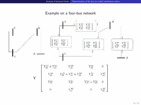
Example on a four-bus network
10 / 16
Analysis of balanced faults Determination of the bus (or nodal) admittance matrix
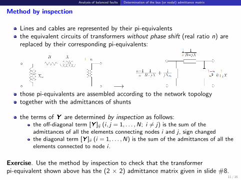
Method by inspection
Lines and cables are represented by their pi-equivalentsthe equivalent circuits of transformers without phase shift (real ratio n) arereplaced by their corresponding pi-equivalents:
−→those pi-equivalents are assembled according to the network topologytogether with the admittances of shunts
the terms of Y are determined by inspection as follows:the off-diagonal term [Y ]ij (i , j = 1, . . . ,N; i 6= j) is the sum of theadmittances of all the elements connecting nodes i and j , sign changedthe diagonal term [Y ]ii (i = 1, . . . ,N) is the sum of the admittances of all theelements connected to node i .
Exercise. Use the method by inspection to check that the transformerpi-equivalent shown above has the (2 × 2) admittance matrix given in slide #8.
11 / 16

Analysis of balanced faults Determination of the bus (or nodal) admittance matrix
Computation of during-fault voltages by superposition
From the during-fault voltages, the current in any component can be computed.
The fault admittance Yf =1
Zfis not included in Y . Indeed:
many possible fault locations have to be analyzed.Including Yf in Y would require modifying Y for each fault location
“solid” faults are considered (as worst cases): Zf = 0 ⇒ Yf →∞cannot be included in Y !
The derivation which follows:
uses the Y matrix relative to the pre-fault configuration of the network
encompasses the case Zf = 0.
12 / 16

Analysis of balanced faults Determination of the bus (or nodal) admittance matrix
Under the combined effect of (I1, I2, . . . , In) and If , the voltages V are such that:
Y V =
I1I2...In0......0
+
0......0−If
0...0
13 / 16

Analysis of balanced faults Determination of the bus (or nodal) admittance matrix
By superposition :V = V
pre + ∆V (1)
with:
Y Vpre =
I1I2...In0......0
and Y ∆V = −If
0......010...0
= −If ef
Vpre : vector of pre-fault bus voltages
∆V : correction accounting for the short-circuit
ef : unit vector (all zero components, except the f -th one equal to 1).
At this step, the value of If is still unknown. . .
14 / 16

Analysis of balanced faults Determination of the bus (or nodal) admittance matrix
Let us solve provisionally:
Y ∆V1
= ef
We have:∆V = −If ∆V
1
Introducing this result in (1):
V = Vpre − If ∆V
1
The f -th component of this relation is:
Vf = V pref − If ∆V
1f
Combining with Vf = Zf If we obtain:
If =V pre
f
∆V1f + Zf
(2)
Substituting in (1), the during fault voltages are given by:
V = Vpre − V pre
f
∆V1f + Zf
∆V1
15 / 16

Analysis of balanced faults Determination of the bus (or nodal) admittance matrix
Relation with Thevenin equivalent
Thevenin equivalent seen from node f :
emf: Eth = V pref
impedance: Zth = voltage at node f when a unit current is injected in thisnode, after the other current injectors have been replaced by open-circuits.Thus:
Zth =[Y−1ef
]f
=[∆V
1]
f= ∆V
1f
Fault current: If =Eth
Zth + Zf=
V pref
∆V1f + Zf
which is nothing but Eq. (2)
Another way to obtain Zth : Zth =[Y−1ef
]f
=[Y−1]
ff= [Z ]ff
Z is called the nodal impedance matrix16 / 16


![Job Analysis Step by Step Guide - bnhexpertsoft.com · model. [Mission Analysis, Competency Analysis, System Analysis, Job Task Analysis and Knowledge/Skill Gap Analysis]. Module](https://img.pdfslide.us/doc/110x75/5e6efaea7135b4624d2ba2da/job-analysis-step-by-step-guide-model-mission-analysis-competency-analysis.jpg)