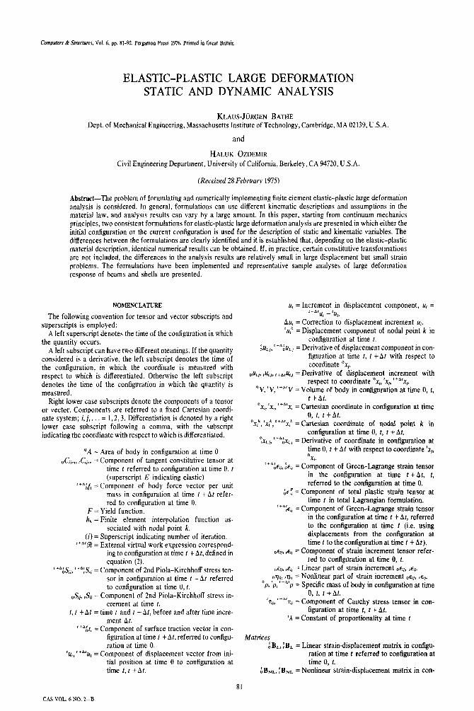
Computers & Sfmfures, Vol. 6, pp. 81-92. Per&mm Press 1976. Printed in Great Britain

ELASTIC-PLASTIC LARGE DEFORMATION STATIC AND DYNAMIC ANALYSIS

KLAUS-J~RGEN BATHE Dept. of Mechanical Engineering, Massachusetts Institute of Technology, Cambridge, MA 02139, U.S.A.

and

HALUK OZDEMIR Civil Engineering Department, University of California, Berkeley, CA 94720, U.S.A.

(Received 28 February 1975)

Abstract-The problem of formulating and numerically implementing finite element elastic-plastic large deformation analysis is considered. In general, formulations can use different kinematic descriptions and assumptions in the material law, and analysis results can vary by a large amount. In this paper, starting from continuum mechanics principles, two consistent formulations for elastic-plastic large deformation analysis are presented in which either the initial configuration or the current configuration is used for the description of static and kinematic variables. The differences between the formulations are clearly identified and it is established that, depending on the elastic-plastic material description, identical numerical results can be obtained. If, in practice, certain constitutive transformations are not included, the differences in the analysis results are relatively small in large displacement but small strain problems. The formulations have been implemented and representative sample analyses of large deformation response of beams and shells are presented.

NOMENCLATURE

The following convention for tensor and vector subscripts and superscripts is employed:

A left superscript denotes the time of the configuration in which the quantity occurs.

A left subscript can have two different meanings. If the quantity considered is a derivative, the left subscript denotes the time of the configuration, in which the coordinate is measured with respect to which is differentiated. Otherwise the left subscript denotes the time of the configuration in which the quantity is measured.

Right lower case subscripts denote the components of a tensor or vector. Components are referred to a fixed Cartesian coordi- nate system; i, j, . = 1,2,3. Differentiation is denoted by a right lower case subscript following a comma, with the subscript indicating the coordinate with respect to which is differentiated.

“A = Area of body in configuration at time 0 ,r&, & = Component of tangent constitutive tensor at

time t referred to configuration at time 0, f (superscript E indicating elastic)

‘+“;jr = Component of body force vector per unit mass in configuration at time t t At refer- red to configuration at time 0.

F = Yield function. h, = Finite element interpolation function as-

sociated with nodal point k. (i) = Superscript indicating number of iteration.

‘+Af% = External virtual work expression correspond- ing to configuration at time t t At, defined in equation (2).

‘+‘+(S 0 I,, ‘+‘:S+ = Component of 2nd Piola-Kirchhoff stress ten- sor in configuration at time t t At referred to configuration at time 0,t.

,,S,, ,S’, = Component of 2nd Piola-Kirchhoff stress in- crement at time t.

t, t t At = time t and t t At, before and after time incre- ment At.

I+&, ot, = Component of surface traction vector in con- figuration at time t t At, referred to contigu- ration at time 0.

‘u. ‘+A’~i = Component of displacement vector from ini- II tial position at time 0 to configuration at time t, t t At.

CAS VOL. 6 NO. 2-B

81

ui = Increment in displacement component, all = ’ +Af& - fUi.

Aui = Correction to displacement increment u,. ‘u,’ = Displacement component of nodal point k in

configuration at time t. *c ,,ui,, = Derivative of displacement component in con-

figuration at time t, t +At with respect to coordinate Ox,.

O~,,i, ,uii, ,+.,,JI~.~ = Derivative of displacement increment with respect to coordinate Ox,, *x,, ‘+*‘xr.

“V, ‘V, t+nr V = Volume of body in configuration at time 0, t, ttAt.

OXi, IX<, ‘+“x, = Cartesian coordinate in configuration at time 0, t, t tAt.

Ox,*, ‘xi*, ‘+A’~,* = Cartesian coordinate of nodal point k in configuration at time 0, t, t t At.

0 t&i,

t+h* 0x,,, = Derivative of coordinate in configuration at time 0, t t At with respect to coordinate ‘xi, OX,.

L+b, O~ii, kij = Component of Green-Lagrange strain tensor

in the configuration at time t t At, t, referred to the configuration at time 0.

;rz= Component of total plastic strain tensor at time t in total Lagrangian formulation.

f+M ,e,, = Component of Green-Lagrange strain tensor in the configuration at time t t At, referred to the configuration at time t (i.e. using displacements from the configuration at time t to the configuration at time t t At).

oe~j, re,, = Component of strain increment tensor refer- red to configuration at time 0, t.

di, dc, = Linear part of strain increment 04,, ,E,,. onij, tnir = Nonlinear part of strain increment Ocg, r~ii.

a ’ P. PT ‘+A’p = Specific mass of body in configuration at time 0, t, t + At.

‘r-- ‘+A’7ji = Component of Cauchy stress tensor in con- ‘,> figuration at time t, t t At.

‘A = Constant of proportionality at time t

Matrices AB,, :Br = Linear strain-displacement matrix in contigu

ration at time t referred to configuration at time 0, t.

;B,,, :B,, = Nonlinear strain-displacement matrix in con-

82 K. .I. BATHE and H. OZDEMIR

figuration at time t referred to configuration at time 0, t.

&, ,C = Tangent material property matrix at time t and referred to configuration at time 0, t

h F, : F = Vector of nodal point forces in configuration at time t referred to configuration at time 0, t.

hKr, :Kr = Linear strain stiffness matrix in configuration at time t referred to configuration at time 0, t.

: K,,, : L = Nonlinear strain stiffness matrix in configura- tion at time t referred to configuration at time 0, t.

M = Mass matrix. ‘+*‘R = Vector of external loads in configuration at

time t t At. : S, i ,!? = 2nd Piola-Kirchhoff stress matrix and vector

in configuration at time t and referred to configuration at time 0.

‘7, ‘i = Cauchy stress matrix and vector in configura- tion at time t.

‘II, ‘+“‘u = Vector of displacements at time t, t + At. u = Vector of incremental displacements at time t.

Au = Vector of corrections to II.

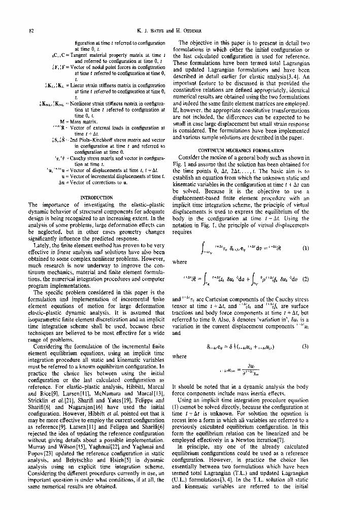
INTRODUCTION

The importance of investigating the elastic-plastic dynamic behavior of structural components for adequate design is being recognized to an increasing extent. In the analysis of some problems, large deformation effects can be neglected, but in other cases geometry changes significantly influence the predicted response.

Lately, the finite element method has proven to be very effective in linear analysis and solutions have also been obtained to some complex nonlinear problems. However, much research is now underway to improve the con- tinuum mechanics, material and finite element formula- tions, the numerical integration procedures and computer program implementations.

The specific problem considered in this paper is the formulation and implementation of incremental finite element equations of motion for large deformation elastic-plastic dynamic analysis. It is assumed that isoparametric finite element discretization and an implicit time integration scheme shall be used, because these techniques are believed to be most effective for a wide range of problems.

Considering the formulation of the incremental finite element equilibrium equations, using an implicit time integration procedure all static and kinematic variables must be referred to a known equilibrium configuration. In practice the choice lies between using the initial configuration or the last calculated configuration as reference. For elastic-plastic analysis, Hibbitt, Marcal and Rice [9], Larsen [ll], McNamara and Marcal [13], Stricklin et al.[21], Sharifi and Yates[19], Felippa and Sharifi[6] and Nagarajan[l6] have used the initial configuration. However, Hibbitt et al. pointed out that it may be more effective to employ the current configuration as reference[9]. Larsen[l l] and Felippa and Sharifi[6] rejected the idea of updating the reference configuration without giving details about a possible implementation. Murray and Wilson[lS], Yaghmai[22] and Yaghmai and Popov[23] updated the reference configuration in static analysis, and Belytschko and Hsieh[S] in dynamic analysis using an explicit time integration scheme. Considering the different procedures currently in use, an important question is under what conditions, if at all, the same numerical results are obtained.

The objective in this paper is to present in detail two formulations in which either the initial configuration or the last calculated configuration is used for reference. These formulations have been termed total Lagrangian and updated Lagrangian formulations and have been described in detail earlier for elastic analysis[3,4]. An important feature to be discussed is that provided the constitutive relations are defined appropriately, identical numerical results are obtained using the two formulations and indeed the same finite element matrices are employed. If, however, the appropriate constitutive transformations are not included, the differences can be expected to be small in case large displacement but small strain response is considered. The formulations have been implemented and various sample solutions are described in the paper.

CONTINUUM MECHANICS FORMULATION

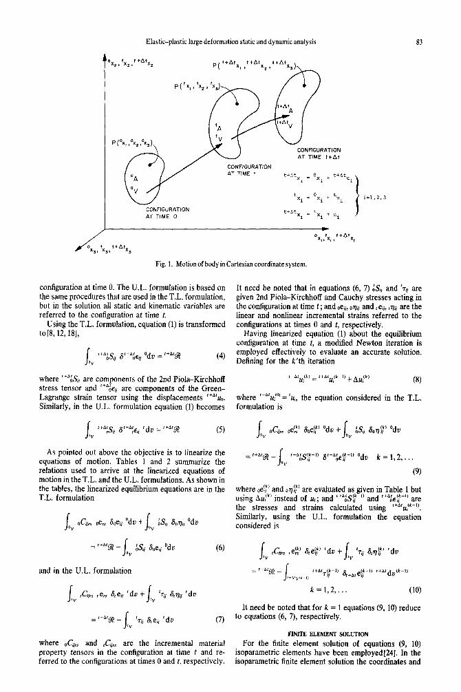
Consider the motion of a general body such as shown in Fig. 1 and assume that the solution has been obtained for the time points 0, At, 2At,. . . , t. The basic aim is to establish an equation from which the unknown static and kinematic variables in the configuration at time t t At can be solved. Because it is the objective to use a displacement-based finite element procedure with an implicit time integration scheme, the principle of virtual displacements is used to express the equilibrium of the body in the configuration at time t t At. Using the notation in Fig. 1, the principle of virtual displacements requires

(1)

where

and ‘+“‘~,i are Cartesian components of the Cauchy stress tensor at time t t At, and ?tk and I+‘& are surface tractions and body force components at time t t At, but referred to time 0. Also, 8 denotes ‘variation in’, Sur is a variation in the current displacement components ‘i”ur and

where

(3)

au, -_ *+atUl."> - a'+a'X,n

It should be noted that in a dynamic analysis the body force components include mass inertia effects.

Using an implicit time integration procedure equation (1) cannot be solved directly, because the configuration at time t t At is unknown. For solution the equation is recast into a form in which all variables are referred to a previously calculated equilibrium configuration. In this form the equilibrium relation can be linearized and be employed effectively in a Newton iteration[7].

In principle, any one of the already calculated equilibrium configurations could be used as a reference configuration. However, in practice the choice lies essentially between two formulations which have been termed total Lagrangian (T.L.) and updated Lagrangian (U.L.) formulations[3,4]. In the T.L. solution all static and kinematic variables are referred to the initial

Elastic-plastic large deformation static and dynamic analysis 83

I CONFIGURATION AT TIME 0

t+Atx. = tX. I 1 + ui

c

ox,,+x,,++A+x, t+At

3

Fig. 1. Motion of body in Cartesian coordinate system.

configuration at time 0. The U.L. formulation is based on the same procedures that are used in the T.L. formulation, but in the solution all static and kinematic variables are referred to the configuration at time t.

Using the T.L. formulation, equation (1) is transformed to@, 12, 181,

I ov ‘+“& St+*& Odv = ‘+A’W (4)

where ‘+‘:Sij are components of the 2nd Piola-Kirchhoff stress tensor and ‘+“& are components of the Green- Lagrange strain tensor using the displacements r+A’uk. Similarly, in the U.L. formulation equation (1) becomes

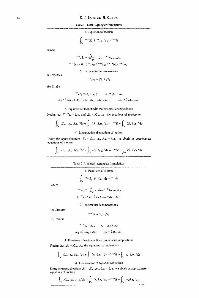
As pointed out above the objective is to linearize the equations of motion. Tables 1 and 2 summarize the relations used to arrive at the linearized equations of motion in the T.L. and the U.L. formulations. As shown in the tables, the linearized equilibrium equations are in the T.L. formulation

I OY oCiirs s, So% ‘dv +

I 9 & 6oqi “dv

= t+ditgy _

I QY & Soeii “dv (6)

and in the U.L. formulation

I I

‘V C. e &e, ‘dv + l,,S f Is

I ‘v ‘rij S,q, ‘dv

= L+%! - I

‘v *Q Sreii ‘dv (7)

where oCii,s and ,C& are the incremental material property tensors in the configuration at time t and re- ferred to the configurations at times 0 and t, respectively.

It need be noted that in equations (6, 7) & and l~ii are given 2nd Piola-Kirchhoff and Cauchy stresses acting in the configuration at time t ; and oeii, oqii and , eii, *vii are the linear and nonlinear incremental strains referred to the configurations at times 0 and t, respectively.

Having linearized equation (1) about the equilibrium configuration at time t, a modified Newton iteration is employed effectively to evaluate an accurate solution. Defining for the k’th iteration

r+Atl(i(k) = l+AtuI(k-I) + Au/k’ (8)

where ‘+*‘~i(‘) = *Us, the equation considered in the T.L. formulation is

I o C

QY iirs Oers (Ir) 6oea’ ‘dv +

I ov :& S&;’ ‘dv

= 1+atg _

I “V

t+A;S{;-‘) S’+A;Ey;-‘) Odv k = 1,2,. . .

(9)

where ,e$’ and OV!~) are evaluated as given in Table 1 but using AU/~’ instead of ui; and *‘“&k#-” and ‘+*&{;-” are the stresses and strains calculated using r+a’~!k-‘). Similarly, using the U.L. formulation the equation considered is

I ‘V ,& ,ej!’ &et’ ‘dv t

I ‘V ‘q &T$ ‘do

= r+Atg _

I l+Arv,t-l) l+Af$-I) a,+Are;;-l’ l+Al&,(k-1)

k=1,2,... (10)

It need be noted that for k = 1 equations (9, 10) reduce to equations (6, 7), respectively.

FINITE ELEMENT SOLUTION

For the finite element solution of equations (9, 10) isoparametric elements have been employed[24]. In the isoparametric finite element solution the coordinates and

K. J. BATHE and H. OZDEMIR

Table 1. Total Latvian fo~ulation

where

(a) Stresses

1. Equations of motion

(b) Strains

3. ~quationsof motion w~thincrementaldecom~os~tions

Noting that S’+*& = &,E~~ and O&j = ,&,, *c, the equa~ons of motion are

4, Linea~2ation of equations of motion

Using the approximations OSji =&&, oeiit &eii = &e, we obtain as approximate equations of motion

Table 2. undated Lagraagiaa formulation

I. Equations of motion

where

(a) Stresses

2. Incremental decompositions

(b) Strains

3. equations of motion with incremental decompositions

Noting that & = ,Cii,, ,e, the equations of motion are

4. Linearization of equatjons of motion

Using the approximations ,S, = ,C,,, c e,s, be, = 8, e, we obtain as approximate equations of motion

Elastic-plastic large deformation static and dynamic analysis 85

displacements of an element are interpolated using

j=1,2,3 (11)

li=,

‘~,=~h~‘u:;Au,=~h~Au: j=1,2,3 (12) k=l k=l

where ‘.x: is the coordinate of nodal point k correspond- ing to direction j at time 0, ‘x;, ‘+“x:, ‘u: and AU; are defined similarly, hr is the interpolation function corres- ponding to nodal point k, and N is the number of nodal points of the element. Using these interpolations to evaluate equations (9, 10) and taking into account that in dynamic analysis the body force components include inertia forces, the matrix equilibrium equation for a single element is in the T.L. formulation

(;KL +~KNL)Au(k)=f+AIR_r+A~F(k-t)_~ t+Ar$k)

k = 1,2,3.. . (13)

where iKL and iKNL are the linear and nonlinear strain stiffness matrices, r+AfR is the vector of externally applied nodal point loads, ‘+‘~I?‘-” is a vector of nodal point forces equivalent to the current element stresses, M is the mass matrix and AU”’ is a vector of nodal point displacement increments, with ‘+ar~(k) = f+A*~(k-l) + Au”‘. The vector of nodal point accelerations is evaluated differently depending on the time integration scheme used.

Considering next the U.L. formulation the equilibrium

equations to be solved are

(:KL t :KNL)h(lr) = ““‘R

_ ::“,:p-‘) _ M’+A’$‘) k = 1, 2, 3. . .

(14)

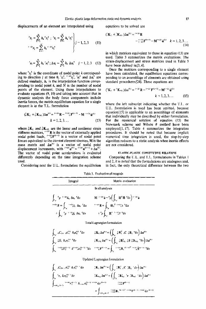
in which matrices equivalent to those in equation (13) are used. Table 3 summarizes the matrix evaluations. The strain-displacement and stress matrices used in Table 3 have been defined in[3,4].

Once the matrices corresponding to a single element have been calculated, the equilibrium equations corres- ponding to an assemblage of elements are obtained using standard procedures[24]. These equations are

(‘KL + fKNL)AU(k) = t+AfR_ f+AIF(k-I)_Mt+At$k)

k=1,2,3... (15)

where the left subscript indicating whether the T.L. or U.L. formulation is used has been omitted, because equation[l5] is applicable to an assemblage of elements that individually may be described by either formulation. For the numerical solution of equation (15) the Newmark scheme and Wilson 0 method have been employed[l, 171. Table 4 summarizes the integration procedures. It should be noted that because implicit numerical time integration is used, the step-by-step algorithm reduces to a static analysis when inertia effects are not considered.

ELASTIC-PLASTIC CONSTITUTIVE RELATIONS

Comparing the U.L. and T.L. formulations in Tables 1 and 2, it is noted that the formulations are analogous and, in fact, the only theoretical difference between the two

Table 3. Evaluation of integrals

Integral Matrix evaluation

86 K. .I. BATHE and H. OZDEMIR

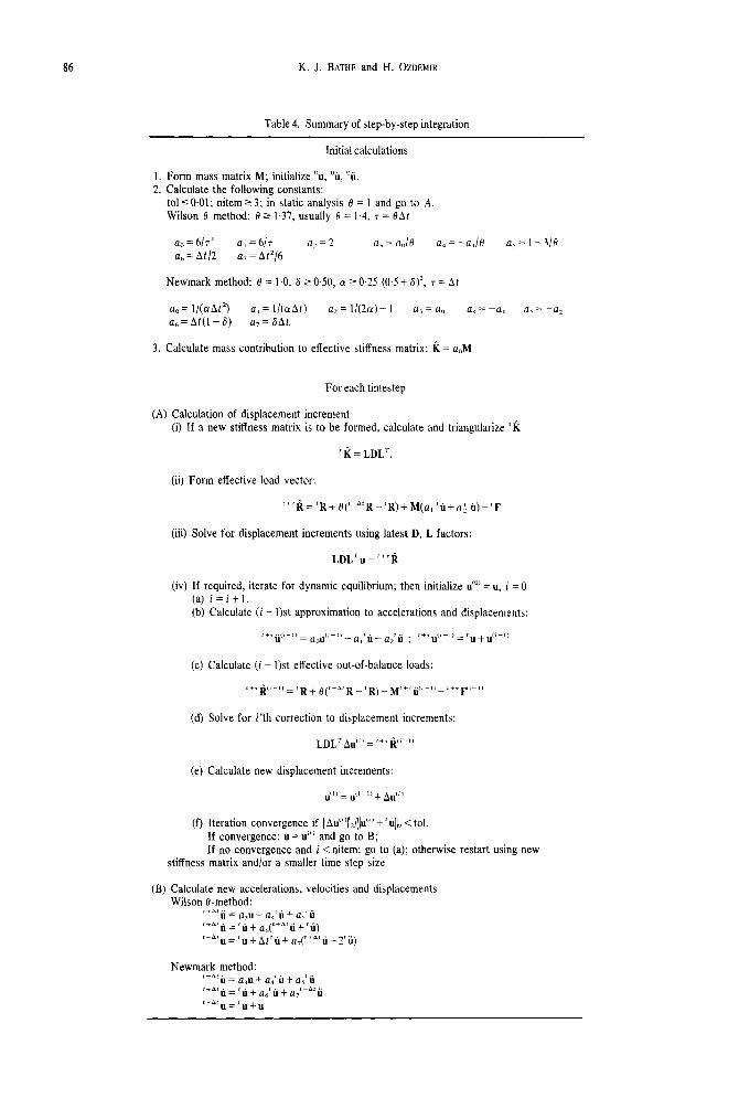
Table 4. Summary of step-by-step integration

Initial calculations

Form mass matrix M; initialize “u, “h, “ii. Calculate the following constants: to1 5 0.01; nitem 2 3; in static analysis 0 = 1 and go to A. Wilson .9 method: 0 z 1.37, usually 0 = 1.4, 7 = BAt

a0 = 6/r’ a, =6/1 a2=2 a, = a,,/0 a, = -a,/0 a, = 1 - 3/0 as=At/2 a, = At216

Newmark method: tJ = 1.0, S 20.50, (Y 2 0.25 (0.5 t 6)2, 7 = At

aa = l/(crAt*) a, = l/(oAf) a* = 1/(2a) - I a, = a, a4 = -a, a, = -a2 ah = At(l - 6) a, = SAt.

Calculate mass contribution to effective stiffness matrix: K = a,M

For each timestep

(A) Calculation of displacement increment (i) If a new stiffness matrix is to be formed, calculate and triangularize ‘K

‘K=LDL’.

(ii) Form effective load vector:

(iii) Solve for displacement increments using latest D, L factors:

(iv) If required, iterate for dynamic equilibrium; then initialize u’“’ = u, i = 0 (a) i=i+l. (b) Calculate (i - 1)st approximation to accelerations and displacements:

“‘$-“= ao”“?l’_a,‘h_a,‘ii ; f+r”‘l-n=1”+“‘I-I

(c) Calculate (i - 1)st effective out-of-balance loads:

“++” = LR+ ,(,+A, R_‘R)_M”‘ii”~“_“~~~~-,~

(d) Solve for i’th correction to displacement increments:

(e) Calculate new displacement increments:

(f) Iteration convergence if ~JAu"'~~&"' t ' u]j2 < tol. If convergence: u = tt(j’ and go to B; If no convergence and i < nitem: go to (a); otherwise restart using new

stiffness matrix and/or a smaller time step size

(B) Calculate new accelerations, velocities and displacements Wilson B-method:

@‘h= o “+a ‘h+a ‘ii I+a.U=‘;+a,;+&‘ii;,ii) “~‘“=‘“+At’li+a,(‘+“‘u+2’ii)

Newmark method: ““‘it= a,ut a,‘it+a,‘ii “b’ti=,t.t+a,‘i+a,‘+“‘ii I*Altt=‘“+U

Elastic-plastic large deformation static and dynamic analysis 87

formulations lies in the choice of different reference configurations for kinematic and static variables. Indeed, if in the numerical solution the appropriate constitutive tensors are used, the evaluation of the corresponding integraIs in equations (67) results into the same matrices and thus identical response is predicted using either formulation. The conditions for obtaining the same equations are that the stresses must be related as given in Tables 1 and 2 and the relation between the constitutive tensors must be as follows,

These relations are precisely the kinematic transforma- tions required for the integrals in equations (6, 7) to be identical. Any differences in response calculations would then lie in the de~nition of ,Cif,$ or o(&. However, in practice, the transfo~ations in equations (16, 17) add to the total computational effort required for solution. Therefore, the aim is to formulate the elastic-plastic constitutive relations directly corresponding to the specific kinematic nonlinear formulation used, and the following two constitutive formulations have been im- pIemented and ev~uated in this work. The basic ingredients of the constitutive relations are those used in small displacement analysis; namely, in addition to the elastic stress-strain relations, the following assump tions are employed: (1) a yield condition, which specifies the state of multiaxial stress corresponding to start of plastic flow; (2) a flow rule relating plastic strain increments to the current stresses and stress increments subsequent to yielding; and (3) a h~dening rule, which specifies how the yield condition is modified during plastic flow [8].

Total Lagrangian formulation For an elastic-plastic material, the constitutive rela-

tions depend on the complete stress and strain history. At any time between the discrete time points t and t + Ar the elastic-plastic material behavior is therefore described in the T.L. formulation using

0)

where d@Sj and doem are differenti~ increments in 2nd Piola-Kirchhoff stresses and Green-Lagrange strains, respectively, and &i,s is the elastic-plastic constitutive tensor at the current stress and strain conditions. Referring to Tables 1 and 3 and equation (13), it is noted that in the caiculation of the linear strain stiffness matrix iKL, the following approximate relation is employed

OS+ = OCiirs oers (1%

where oers is the linear part of ~e,~, and ,&i, is the stress-strain relation at time t. However, in the equilib- rium iterations the total incremental strains are calculated using

oErr - IL) _ “I;e$‘_ f 06s (201

and then, because 0&S is a function of the stresses and strains,

To evaluate the integral in equation (21) Euler’s method has been used[7]. The stresses corresponding to ‘+$e$’ are then

t+$# = ;S, +& (221

The above description shows that basically the material tensor ,,C& need be evaluated for a given stress and strain state. Consider the calculation of &$ corresponding to ,& and &. In the investigation carried out isothermal and elastic-perfectly plastic or isotropic hardening conditions have been assumed. In this case the initial and subsequent yield condition is

F(iSij, ‘K) = 0 (23)

where ‘K is a hardening parameter that depends on the total plastic strains &g. The total plastic strain is obtained by addition of the incremental plastic strains d&

doe;= d,eii -d& (24

where doe: is the elastic part of the differential increment in strain 4~. Assuming an associated flow rule

and because F = 0 during plastic deformation

0.6)

The stress increments are catculated using

do& = nC;?$ d& (27)

where ,& is a component of the elasticity tensor relat- ing 2nd Piola-Kirchhoff stresses to Green-Lagrange strains [3].

Equations (23-27) enable the calculation of the compo- nents of the constitutive tensor oCii,s in equation (18) in the usual way 181,

It may be noted that once ‘+‘$Sjf) has been evaluated and the iteration converged, Cauchy stresses are calcu- lated as given in Table 1 whenever stress output is required.

Updated Lagra~gia~ fo~ulation In the U.L. formulation the elastic-plastic material

response is described using

d& = J&s d, ers (2%

where d,S, and dIers are differential increments in the 2nd

88 K. J. BATHE and H. OZDEMIR

Piola-Kirchhoff stress referred to the configuration at time t and the linear part of ,Q, respectively. In analogy to the T.L. formulation, in the calculation of the linear strain stiffness matrix :KL, the relation used is

& = C- e f t,rs f 0 (30)

A main difference appears in the calculation of stresses. The solution of equation (14) yields A@ and thus corres- ponding strain components ,e!:’ can be calculated and

where (C,,,.? is a function of the current total stress and strain conditions. Cauchy stresses are then evaluated using

and

‘+“;s!;) ZZ tr,, +,s;;’ (32)

The calculation of the constitutive relations is carried out as in the T.L. formulation but using Cauchy stresses and the small displacement strain increments ,e,,. It should be noted that in the evaluation total plastic strains are obtained by addition of the plastic components of , e, occurring in each time step. The U.L. formulation is therefore quite similar to the calculation of elastic-plastic constitutive relations in small displacement analysis, but to take large displacements into account the transforma- tion in equation (33) is used for stress calculations.

Comparison of formulations On comparing the evaluation of the elastic-plastic

constitutive relations in the U.L. and T.L. formulations, it is noted that different basic assumptions are used. In the T.L. formulation the elastic properties, the yield function and flow rule are defined in the 2nd Piola-Kirchhoff stress space whereas in the U.L. formulation the Cauchy stress space is employed. Under large displacement and large strain conditions, it would therefore be necessary to specify the appropriate elasticity constants, yield stresses and hardening constants. If the same material constants were used large differences between the response pre- dicted using the T.L. and U.L. formulations would, in general, be observed. However, if only moderate defor- mations are considered the response predicted using the U.L. and T.L. formulations can be expected not to differ a great deal. Namely, for moderate deformations

‘7:; = is, + 0 (&&,l &J) (34)

where o signifies ‘of order’. But then considering the calculation of the elastic-plastic incremental constitutive relations, it is noted that products of stresses are emp- loyed and hence the differences in the elements of the stress-strain matrices used in the T.L. and U.L. formula- tions will be small.

Considering the implementation of the two formula- tions, it is noted that the T.L. formulation is programmed more easily. Namely, in this case large displacement analysis is a simple extension of small displacement analysis in that the same subroutine which calculates the

material matrix in small displacement analysis can be used without modification for large displacement conditions. It is only necessary to work with 2nd Piola-Kirchhoff stresses and Green-Lagrange strains instead of conven- tional small displacement strains and stresses.

SAMPLE SOLUTIONS

To implement the T.L. and U.L. formulations described above program NONSAP was employed[2]. The program is available with the T.L. formulation for elastic-plastic analysis and thus had to be modified for the U.L. formulation.

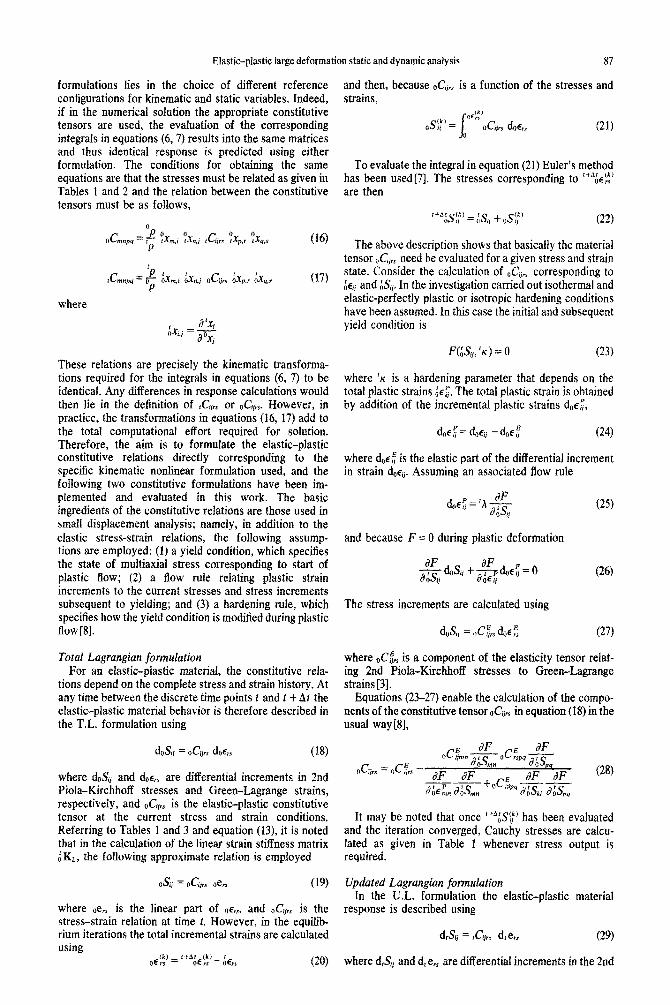
Static large displacement analysis of a cantilever The cantilever in Fig. 2 was analyzed for a uniformly

distributed load using five g-node plane stress isoparamet- ric elements. The material of the cantilever was assumed to be isotropic and linear elastic. An analytical solution for the response of the cantilever was given by Holden [IO].

The purpose of this analysis was to compare the Holden solution with the response predicted using the T.L. and U.L. formulations. Since the beam is elastic, to prevent plastic response the yield stress of the material was selected sufficiently high. It should be noted that in this case the same material constants have been employed in both formulations.

The response of the cantilever using the T.L. and U.L. formulations and 100 equal load steps is shown in Fig. 3, in which Holden’s solution is also given. It is seen that for the accuracy with which the response can be presented in the figure all three solutions are identical.

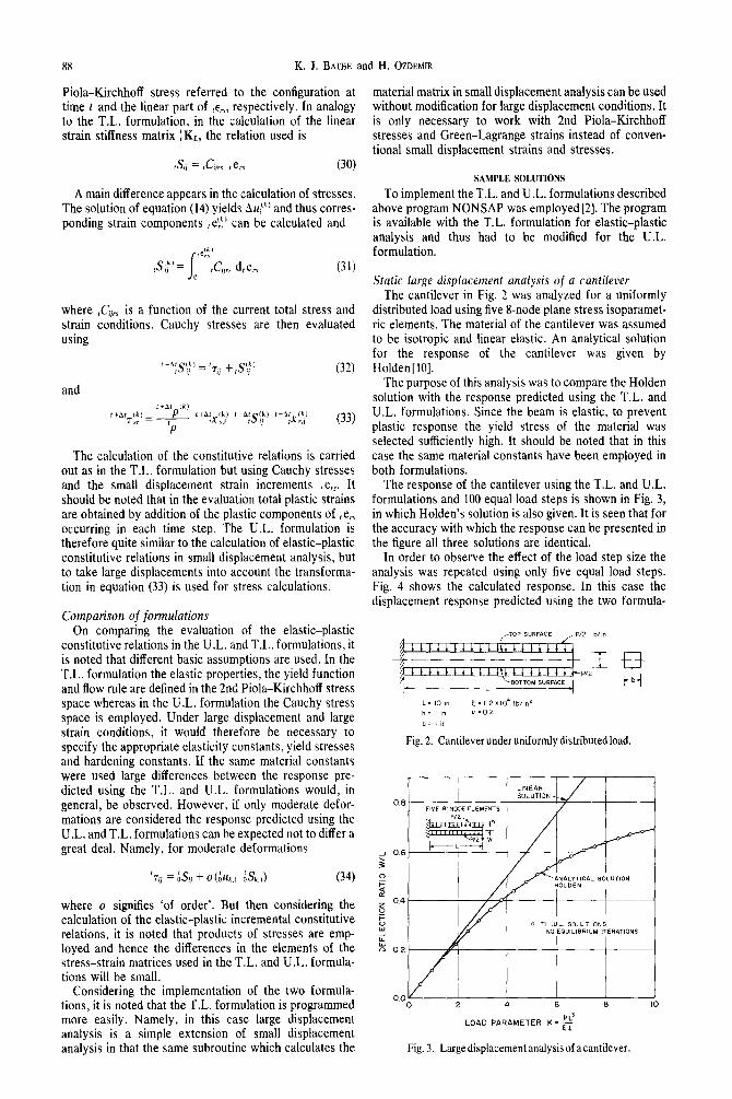
In order to observe the effect of the load step size the analysis was repeated using only five equal load steps. Fig. 4 shows the calculated response. In this case the displacement response predicted using the two formula-

L= IO I” E~12xlO’lb/,n~ h= 8,” u=o2

b= I,”

Fig. 2. Cantilever under uniformly distributed load.

0.0 0 2 4 6 8 IO

LOAD PARAMETER K = j$

Fig. 3. Large displacement analysis of a cantilever.

Elastic-plastic large deformation static and dynamic analysis 89

ov 2 4 6 8 IO

LOAD PARAMETER K = 2’

Fig. 4. Large displacement analysis of a cantilever, comparison of nonlinear formulations.

tions is significantly different, because the incremental solution using either formulation was not obtained accurately.

Static large displacement analysis of a spherical shell The elastic spherical shell shown in Fig. 5 was analyzed

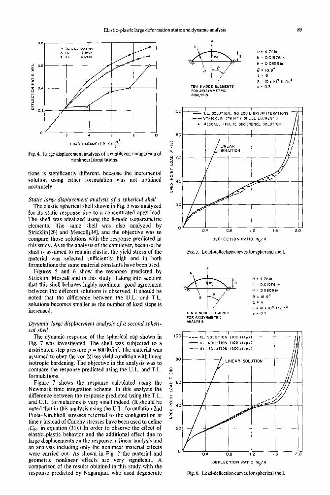
for its static response due to a concentrated apex load. The shell was idealized using the g-node isoparametric elements. The same shell was also analyzed by Stricklin[20] and Mescall[l4], and the objective was to compare those solutions with the response predicted in this study. As in the analysis of the cantilever, because the shell is assumed to remain elastic, the yield stress of the material was selected sufficiently high and in both formulations the same material constants have been used.

Figures 5 and 6 show the response predicted by Stricklin, Mescall and in this study. Taking into account that this shell behaves highly nonlinear, good agreement between the different solutions is observed. It should be noted that the difference between the U.L. and T.L. solutions becomes smaller as the number of load steps is increased.

Dynamic large displacement analysis of a second spheri- cal shell

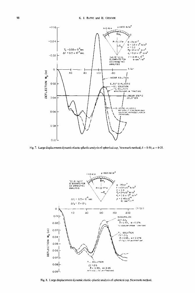
The dynamic response of the spherical cap shown in Fig. 7 was investigated. The shell was subjected to a distributed step pressure p = 600 lb/in’. The material was assumed to obey the von Mises yield condition with linear isotropic hardening. The objective in the analysis was to compare the response predicted using the U.L. and T.L. formulations.

Figure 7 shows the response calculated using the Newmark time integration scheme. In this analysis the difference between the response predicted using the T.L. and U.L. formulations is very small indeed. (It should be noted that in this analysis using the U.L. formulation 2nd Piola-Kirchhoff stresses referred to the configuration at time t instead of Cauchy stresses have been used to define ,C,,,$ in equation (31).) In order to observe the effect of elastic-plastic behavior and the additional effect due to large displacements on the response, a linear analysis and an analysis including only the nonlinear material effects were carried out. As shown in Fig. 7 the material and geometric nonlinear effects are very significant. A comparison of the results obtained in this study with the response predicted by Nagarajan, who used degenerate

P

TEN 8 NODE ELEMENTS FOR AXISYMMETRIC ANALYSIS

R= 476in

h = 0.01576 I”

H = 0.0659 in

6 = lo.9o

X= 6

E = IO x IO’ lb/,“’ Y = 0.3

100 I I I I

- T.L. SOLUTION, NO EQUILIBRIUM ITERATIONS -- STRICKLIN (THIRTY SHELL ELEMENTS)

. MESCALL (FINITE DIFFERENCE SOLUTION)

DEFLECTION RATIO W,/H

Fig. 5. Load-deflection curves for spherical shell.

R = 476in

h = 0.01576 I”

H = ooFl591n

8; 109O

A’6

E = IO x IO’ lb/in’

TEN 8 NODE ELEMENTS Y = 0.3 FOR AXlSYMMETRlC ANALYSIS

100

- UL SOLUTION (100 step.1

-- UL. SOLUTION 1200steps)

60 NEAR SOLUTION

E I a o 60

z

!G 0 a 40

c

:

20

0 0.4 0.6 1.2 16 2.0

DEFLECTION RATIO W,/H

Fig. 6. Load-deflection curves for spherical shell.

K. J. BATHE and H. OZDEMIR

-004

-0 02

z

0

so

5 002 F

Y

i:

x 004

006

0 06

0 IO

Tf = 0.55 x Id3sec

At = 0.5 x Idgsec

I I I

\

40 60

h=o 41 I” p=bOO lb/i?

u L SOLUTlON TL SOLUTlON WITH E0”ILlBRlUM IiERiliiONS

LINEAR STATIC

TEN e-NODE P = 2 45 x c4 ELEMENTS FOR lb-oecz/,n4 AXlSYMMETRlC ANALYSIS

1 t/At

160 I

LINEAR SOLUTION

I ELASTIC-PLASTIC

Fig. 7. Large displacement dynamic elastic-plastic analysis of spherical cap, Newmark method, 6 = 0.50, (Y = 0.25.

0.02

c 003 ;

P 004

$ F 0.05

0

Y 006

k 0.07

0.06

009

a :2667’

E = IO 5x1061b/,n2

v=o3 my= 24~10~ lb/in’

et = 0 21 x IO6 lb/in’

p = 2 45 x 10-4 lb-secz/tn4

At,= 2xAt,

I I I I I (t/At,)

40 60 I20 I60 200

I \ T L SOLUTION

Fig. 8. Large displacement dynamic elastic-plastic analysis of spherical cap, Newmark method

Elastic-plastic large deformation static and dynamic analysis 91

isoparametric elements and (Y = 0,276, 6 = 0.55 in the Newmark method is given in Fig. 8[16].

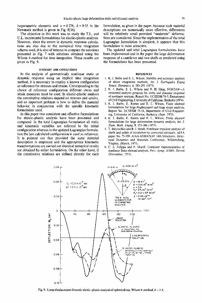
The objective in this work was to study the T.L. and U.L. incremental formulations for elastic-plastic analysis. However, since the errors in dynamic response calcula- tions are also due to the numerical time integration scheme used, it is also of interest to compare the solutions presented in Fig. 7 with solutions obtained using the Wilson o-method for time integration. These results are given in Fig. 9.

SUMMARY AND CONCLUSIONS

In the analysis of geometrically nonlinear static or dynamic response using an implicit time integration method, it is necessary to employ a known configuration as reference for stresses and strains. Corresponding to the choice of reference configuration different stress and strain measures must be used. In elastic-plastic analysis the constitutive relations depend on stresses and strains, and an important problem is how to define the material behavior in conjunction with the specific kinematic formulation used.

In this paper two consistent and effective formulations for elastic-plastic analysis have been presented and compared. In the total Lagrangian formulation all static and kinematic variables are referred to the initial configuration whereas in the updated Lagrangian formula- tion the last calculated configuration is used as reference. It is pointed out that provided the same material description is employed and the appropriate kinematic transformations are carried out identical numerical results are obtained by either formulation. On the other hand, if the constitutive relations are defined directly for each

-0 06 r Tt =055~lO-~sec

At =05x10-'set

formulation, as given in the paper, because such material descriptions are numerically more effective, differences will be relatively small provided “moderate” deforma- tions are considered. Since the implementation of the total Lagrangian formulation is simplest, it appears that this formulation is most attractive.

The updated and total Lagrangian formulations have been implemented and in the paper the large deformation response of a cantilever and two shells as predicted using the formulations has been presented.

REFERENCES

1. K. J. Bathe and E. L. Wilson, Stability and accuracy analysis of direct integration methods, Int. J. Earthquake Engng Struct. Dynamics, 1, 283-291 (1973).

2. K. J. Bathe, E. L. Wilson and R. H. Iding, NONSAP-A structural analysis program for static and dynamic response of nonlinear systems, Report No. UCSESM 74-3, Department of Civil Engineering, University of California, Berkeley (1974).

3. K. J. Bathe, E. Ramm and E. L. Wilson, Finite element formulations for large displacement and large strain analysis, Report No. UCSESM 73-14, Department of Civil Engineer- ing, University of California, Berkeley (Sept. 1973).

4. K. J. Bathe, E. Ramm and E. L. Wilson, Finite element formulations for large deformation dynamic analysis, Int. J. Num. Meth. Engng, 9, 353-386 (1975).

5. T. Belytschko and B. J. Hsieh, Nonlinear transient analysis of shells and solids of revolution by convected elements, AIAA paper No. 73-359, AIAA-ASME/SAE 14th Structures, Struc- tural Dynamics and Materials Conference, Williamsburg, Virginia, (March, 1973).

6. C. A. Felippa and P. Sharifi, Computer implementation of nonlinear finite element analysis, Proc. Symp. ASME, Detroit (November, 1973).

h-0.41 I” ~‘600 lb/,“’

l + = 0 21 x IO6 lb/d

TEN 6 NODE ,D = 2.45 I IO-”

ELEMENTS FOR lb-ad/in4

I I AXISYMMETRIC ANALYSIS

006

I I I I I I

t/At

40 60 120 160 200

ELASTIC-PLASTIC

Fig. 9. Large displacement dynamic elastic-plastic analysis of spherical cap, Wilson e-method, 8 = 1.4.

92 K. J. BATHE and H. OZDEMIR

C. E. Frobera, Introduction to Numerical Analvsis. Addison- 17. R. E. Nickel], Direct inteeration methods in structural

10.

11.

12.

13.

14.

15.

16.

Wesley, Reading, Mass. _

Y. C. Fung, Foundations of Solid Mechanics, Prentice-Hall, 18 Englewood Cliffs, New Jersey (1965). H. D. Hibbitt, P. V. Marcal and J. R. Rice, Finite element 19 formulation for problems of large strain and large displace- ments, Int. J. Solids Struct. 6, 1069-1086 (1970). J. T. Holden, On the finite deflections of thin beams, Int. J. Solids Struct. 8, 1051-1055 (1972). P. K. Larsen. Large displacement analysis of shells of 20 revolution. including creep, plasticity and viscoelasticity, Report No. UCSESM 71-22, Department of Civil Engineer- ing, University of California, Berkeley (1971). L. E. Malvern, Introduction to the Mechanics of a Continuous ?I

Medium, Prentice-Hall, Englewood Cliffs, New Jersey. (1969). J. F. McNamara and P. V. Marcal, Incremental stiffness method for finite element analysis of the nonlinear dynamic problem, In Numerical and Computer Methods in Structural Mechanics, Fenves, Perrone, Robinson and Schnobrich, (Eds.) Academic Press, New York (1973). 22. J. F. Mescall, Large deflections of spherical shells under concentrated loads, J. Appl. Mech. 32, 936-938 (1965). D. W. Murray and E. L. Wilson, Finite element large. deflection analysis of plates, ASCE, J. Engng. Mech. Div. 95, 23. 143-165 (1969). S. Nagarajan, Nonlinear static and dynamic analysis of shells of revolution under axisymmetric loading, Report No. 24. UCSESM 73-11, Department of Civil Engineering, University of California, Berkeley (1973).

dynamics, ASCE, L Engng. Mech. Div. 99, 303-317, (1973). J. T. Oden, Finite Elements of Nonlinear Continua, McGraw- Hill, New York (1972). P. Sharifi and D. N. Yates, Nonlinear thermo-elastic-plastic and creep analysis by the finite element method, AIAA-Paper No. 73-358. AIAAIASMEISAE 14th Structures. Structural Dynamics and Materials Conference, Williamsburg, Virginia (March, 1973). J. A. Stricklin, Geometrically nonlinear static and dynamic analysis of shells of revolution, High speed computing of elastic structures, Proc. Symp. IUTAM, University of Liege, pp. 383-411 (August, 1970). J. A. Stricklin, W. A. Von Riesemann, J. R. Tillerson and W. E. Haisler, Static geometric and material nonlinear analysis, Advances in Computational Methods in Structural Mechanics and Design, 2nd U.S.-Japan Seminar in Matrix Methods of Structural Analysis and Design, University of Alabama Press pp. 301-324 (1972). S. Yaghmai, Incremental analysis of large deformations in mechanics of solids with applications to axisvmmetric shells of revolution, Report No..UCSESM 68-17;Department of Civil Engineerina. Universitv of California. Berkelev (1968). S. Yaghmai and-E. P. Pop&, Incremental analysis of large deflections of shells of revolution, Int. J. Solids Struct. 7, 1375-1393 (1971). 0. C. Zienkiewicz, The Finite Element Method in Engineering Science, McGraw-Hill, London (1971).