Embed Size (px)
Citation preview
EL2620 Nonlinear Control
Exercises and HomeworkHenning Schmidt, Karl Henrik Johansson, Krister Jacobsson, Bo Wahlberg,Per Hägg, Elling W. Jacobsen
September 2012
Automatic Control
KTH, Stockholm, Sweden

Contents
Preface 5
1 Homeworks 7
1.1 Report Requirements . . . . . . . . . . . . . . . . . . . . . . . . . . . . . . . . . . . . . . . 71.1.1 Writing your report using Microsoft Word R© . . . . . . . . . . . . . . . . . . . . . . . 71.1.2 Writing your report using LATEX . . . . . . . . . . . . . . . . . . . . . . . . . . . . . 81.1.3 Work in groups of two . . . . . . . . . . . . . . . . . . . . . . . . . . . . . . . . . . 91.1.4 Grading . . . . . . . . . . . . . . . . . . . . . . . . . . . . . . . . . . . . . . . . . . 91.1.5 References . . . . . . . . . . . . . . . . . . . . . . . . . . . . . . . . . . . . . . . . 11
1.2 Homework 1 . . . . . . . . . . . . . . . . . . . . . . . . . . . . . . . . . . . . . . . . . . . 121.3 Homework 2 . . . . . . . . . . . . . . . . . . . . . . . . . . . . . . . . . . . . . . . . . . . 131.4 Homework 3 . . . . . . . . . . . . . . . . . . . . . . . . . . . . . . . . . . . . . . . . . . . 15
2 Exercises 19
2.1 Nonlinear Models and Simulation . . . . . . . . . . . . . . . . . . . . . . . . . . . . . . . . 192.2 Computer exercise: Simulation . . . . . . . . . . . . . . . . . . . . . . . . . . . . . . . . . . 242.3 Linearization and Phase-Plane Analysis . . . . . . . . . . . . . . . . . . . . . . . . . . . . . 262.4 Lyapunov Stability . . . . . . . . . . . . . . . . . . . . . . . . . . . . . . . . . . . . . . . . 302.5 Input-Output Stability . . . . . . . . . . . . . . . . . . . . . . . . . . . . . . . . . . . . . . . 342.6 Describing Function Analysis . . . . . . . . . . . . . . . . . . . . . . . . . . . . . . . . . . . 432.7 Anti-windup . . . . . . . . . . . . . . . . . . . . . . . . . . . . . . . . . . . . . . . . . . . . 512.8 Friction, Backlash and Quantization . . . . . . . . . . . . . . . . . . . . . . . . . . . . . . . 552.9 High-gain and Sliding mode . . . . . . . . . . . . . . . . . . . . . . . . . . . . . . . . . . . 582.10 Computer Exercises: Sliding Mode, IMC and Gain scheduling . . . . . . . . . . . . . . . . . 632.11 Gain scheduling and Lyapunov based methods . . . . . . . . . . . . . . . . . . . . . . . . . . 662.12 Feedback linearization . . . . . . . . . . . . . . . . . . . . . . . . . . . . . . . . . . . . . . 712.13 Optimal Control . . . . . . . . . . . . . . . . . . . . . . . . . . . . . . . . . . . . . . . . . . 742.14 Fuzzy control . . . . . . . . . . . . . . . . . . . . . . . . . . . . . . . . . . . . . . . . . . . 80
3 Solutions 81
3.1 Solutions to Nonlinear Models and Simulation . . . . . . . . . . . . . . . . . . . . . . . . . . 813.2 Solutions to Computer exercise: Simulation . . . . . . . . . . . . . . . . . . . . . . . . . . . 853.3 Solutions to Linearization and Phase-Plane Analysis . . . . . . . . . . . . . . . . . . . . . . 863.4 Solutions to Lyapunov Stability . . . . . . . . . . . . . . . . . . . . . . . . . . . . . . . . . . 903.5 Solutions to Input-Output Stability . . . . . . . . . . . . . . . . . . . . . . . . . . . . . . . . 943.6 Solutions to Describing Function Analysis . . . . . . . . . . . . . . . . . . . . . . . . . . . . 1023.7 Solutions to Anti-windup . . . . . . . . . . . . . . . . . . . . . . . . . . . . . . . . . . . . . 1083.8 Solutions to Friction, Backlash and Quantization . . . . . . . . . . . . . . . . . . . . . . . . 1103.9 Solutions to High-gain and Sliding mode . . . . . . . . . . . . . . . . . . . . . . . . . . . . . 1143.10 Solutions to Computer Exercises: Sliding Mode, IMC and Gain scheduling . . . . . . . . . . 120
3

3.11 Solutions to Gain scheduling and Lyapunov based methods . . . . . . . . . . . . . . . . . . . 1223.12 Solutions to Feedback linearization . . . . . . . . . . . . . . . . . . . . . . . . . . . . . . . . 1263.13 Solutions to Optimal Control . . . . . . . . . . . . . . . . . . . . . . . . . . . . . . . . . . . 1293.14 Solutions to Fuzzy control . . . . . . . . . . . . . . . . . . . . . . . . . . . . . . . . . . . . 133
4

Preface
Many people have contributed to this material in nonlinear control. Originally, it was developed by Bo Bern-hardsson, Karl Henrik Johansson, and Mikael Johansson. Later contributions have been added by HenningSchmidt, Krister Jacobsson, Bo Wahlberg, Elling Jacobsen, Torbjörn Nordling, Per Hägg and Farhad Farokhi.Exercises have also shamelessly been borrowed (stolen) from other sources, mainly from Karl Johan Åström’scompendium in Nonlinear Control and Khalil’s book Nonlinear Systems.
Per Hägg and Elling W. Jacobsen, September 2012
5

6
Chapter 1
Homeworks
1.1 Report Requirements
Your homework reports should be handed-in as a single PDF file containing all the typed answers, figures,tables, and etc. You can prepare this document using both Microsoft Word R© or LATEX. However, there is a setof requirements that your homework should satisfy in order to get considered and subsequently, approved. Inwhat follows, the homework requirements are specified.
In your report, you should first describe the problem in your own words and break it down into subproblems,unless the problem was already broken down into subproblems in the description of the homework. In eachsubproblem you should define a set of questions or tasks which gradually lead you to a solution of the overallproblem. The problem should be described in detail, so that the reader can understand it without reading thedescription of the homework. Then, solve the subproblems in succession and give the solution to the overallproblem at the end, followed by a sentence or two about what you learned from solving the problem. You shouldlead the reader through a detailed solution where you motivate every step, state every theorem, and verify thatthe assumptions are fulfilled. The presentation should be detailed yet clear and concise. You should providea reference (including the page number) for every theorem and result that you are using [2]. Any engineeringstudent with a bachelor’s degree should be able to understand and reproduce the results based on your reportalone. You may not copy-and-paste any text, theorem, or figure except the figures used in the description of thehomework. Only include figures and tables if they fosters the understanding of the solution. Each figure andtable should include a caption, and all the figures and tables should be associated with a reference in the textand placed at the end of your report. Each equation should only be written once and referred to by referencelater when needed. Equations that you do not refer to later may be left unlabeled. You are not allowed to haveany appendix nor attach any Matlab or other code.
You report (excluding the figures and tables) should not be shorter than two pages and longer than fourpages. The reports should contain the names of the students (who have collaborated as a group to solve theproblems and write the report) and their email addresses. The solutions may not be copy-pasted from othersources such as textbooks, internet webpages, or other groups report. You should properly cite all the theorems,texts, or results that you use when creating the report. Plagiarism (i.e., the act of copying someone else ideas,text, or results in any form while presenting it as your own work, particularly without permission1) will bereported to the KTH Disciplinary Board.
Finally, note that deadlines listed on the course page are hard. We will not accept any delays in handing inreports or reviews.
1.1.1 Writing your report using Microsoft Word R©
You should write your report as a double column document. In Microsoft Word R© 2010 release (which I wouldonly refer during this description), you can change the number of columns under the page layout tab. You
1http://en.wiktionary.org/wiki/plagiarism
7
Homework 1 in EL2620 Nonlinear Control
First name1 Last name1
person number
First name2 Last name2
person number
September 22, 2009
Problem
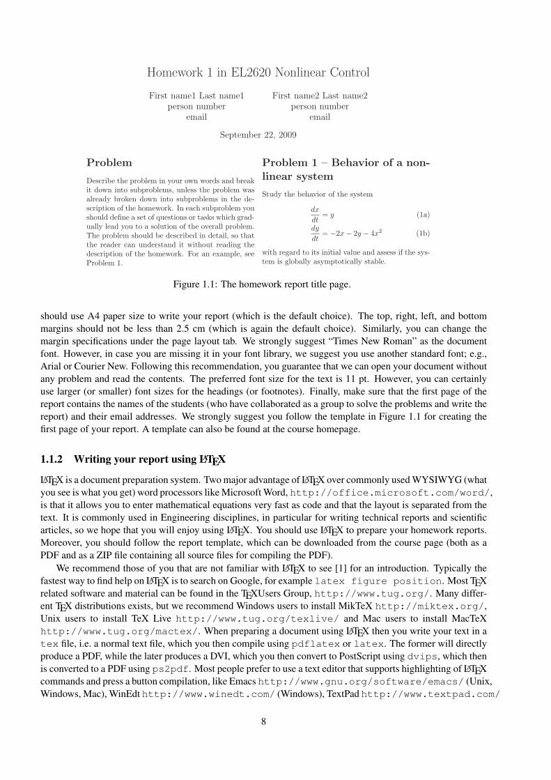
Describe the problem in your own words and breakit down into subproblems, unless the problem wasalready broken down into subproblems in the de-scription of the homework. In each subproblem youshould define a set of questions or tasks which grad-ually lead you to a solution of the overall problem.The problem should be described in detail, so thatthe reader can understand it without reading thedescription of the homework. For an example, seeProblem 1.
Problem 1 – Behavior of a non-
linear system
Study the behavior of the system
dx
dt= y (1a)
dy
dt= −2x− 2y − 4x2 (1b)
with regard to its initial value and assess if the sys-tem is globally asymptotically stable.
We have chosen a solution strategy based on the
Figure 1.1: The homework report title page.
should use A4 paper size to write your report (which is the default choice). The top, right, left, and bottommargins should not be less than 2.5 cm (which is again the default choice). Similarly, you can change themargin specifications under the page layout tab. We strongly suggest “Times New Roman” as the documentfont. However, in case you are missing it in your font library, we suggest you use another standard font; e.g.,Arial or Courier New. Following this recommendation, you guarantee that we can open your document withoutany problem and read the contents. The preferred font size for the text is 11 pt. However, you can certainlyuse larger (or smaller) font sizes for the headings (or footnotes). Finally, make sure that the first page of thereport contains the names of the students (who have collaborated as a group to solve the problems and write thereport) and their email addresses. We strongly suggest you follow the template in Figure 1.1 for creating thefirst page of your report. A template can also be found at the course homepage.
1.1.2 Writing your report using LATEX
LATEX is a document preparation system. Two major advantage of LATEX over commonly used WYSIWYG (whatyou see is what you get) word processors like Microsoft Word, http://office.microsoft.com/word/,is that it allows you to enter mathematical equations very fast as code and that the layout is separated from thetext. It is commonly used in Engineering disciplines, in particular for writing technical reports and scientificarticles, so we hope that you will enjoy using LATEX. You should use LATEX to prepare your homework reports.Moreover, you should follow the report template, which can be downloaded from the course page (both as aPDF and as a ZIP file containing all source files for compiling the PDF).
We recommend those of you that are not familiar with LATEX to see [1] for an introduction. Typically thefastest way to find help on LATEX is to search on Google, for example latex figure position. Most TEXrelated software and material can be found in the TEXUsers Group, http://www.tug.org/. Many differ-ent TEX distributions exists, but we recommend Windows users to install MikTeX http://miktex.org/,Unix users to install TeX Live http://www.tug.org/texlive/ and Mac users to install MacTeXhttp://www.tug.org/mactex/. When preparing a document using LATEX then you write your text in atex file, i.e. a normal text file, which you then compile using pdflatex or latex. The former will directlyproduce a PDF, while the later produces a DVI, which you then convert to PostScript using dvips, which thenis converted to a PDF using ps2pdf. Most people prefer to use a text editor that supports highlighting of LATEXcommands and press a button compilation, like Emacs http://www.gnu.org/software/emacs/ (Unix,Windows, Mac), WinEdt http://www.winedt.com/ (Windows), TextPad http://www.textpad.com/
8
(Windows), TeXShop http://www.uoregon.edu/~koch/texshop/ (Mac), but you may start by us-ing built-in programs like Notepad (Windows), pico (Unix), TextEdit (Mac). If you have trouble, please readthe help files and documents coming with the software, search on the Internet, ask your course mates and readLATEX books.
A short getting you started list:
1. Install a TEX distribution.
2. Download and unzip the report template.
3. Open report_template.tex using a built-in text editor.
4. Produce a PDF by issuing the command pdflatex report_template.tex at the command prompt(Windows) or in the terminal (Unix, Mac) in the directory where you unzipped the report template. Doit three times in a row to get the references correct. This compiles the report template and creates thereport_template.log, report_template.aux and report_template.pdf files in the same directory. Open thePDF and verify that it is identical to the one on the course page.
5. Start writing you report by changing in the report template.
Including vector graphics from Matlab
A bitmap image, e.g. JPEG, TIFF or PNG, has a finite resolution, since the image consists of a limited numberof pixels. Vector graphics, e.g. EPS and PDF, on the contrary consists of objects placed relatively to eachother, which in practice means infinite resolution. Vector graphics can therefore be scaled without any qualityproblems, while a bitmap typically becomes blurred. You should therefore always use vector graphics whenpossible. Note that vector graphics are containers of objects and it is therefore possible to place a bitmap imageas one of the objects, but you should never do this, since it will lead to problems when scaling the figure.
The current pdflatex compiler can include figures in PDF (Portable Document Format), JPEG (JointPhotographic Experts Group), PNG (Portable Network Graphics) and MetaPost, while the latex compileronly can include EPS (Encapsulated PostScript). Matlab figures (http://www.mathworks.com) con-sists of vector graphics, unless you load a bitmap image, so we strongly recommend that you save themas EPS or PDF. You need to set the paper size equal to the figure size or you will typically end up with asmall figure centered on a large paper. The paper size 15 × 10 centimeters is set by issuing the commandset(gcf, ’PaperUnits’, ’centimeters’, ’PaperSize’, [15 10], ’PaperPosition’,
[0 0 15 10]);, see Matlab_code_for_stepresponse_figure.m, which is included in the ZIP file containingthe report template. The paper size, however, only matters for the PDF, since every EPS contains a Bounding-Box that is used by LATEX to define the size of the figure. A simple way to avoid setting the paper size is thereforeto save the Matlab figure as an EPS and then convert it to a PDF using epstopdf. Matlab figures can eitherbe saved by clicking on File and selecting Save As. . . or by issuing the command print -dpdf -noui
-painters FileName to save as a PDF or print -depsc2 -noui -painters -tiff FileName
to save as an EPS. Note the option -noui that removes any user interface control objects from the figure.
1.1.3 Work in groups of two
You should do the homeworks in pairs (more than two students per group will not be accepted). If more thanone student has done homework 1 alone, then a partner will be designated to those who have done it on theirown.
1.1.4 Grading
Every subproblem is graded as either 1 or 0 points. One point is given if at least 95% of the solution iscorrect. To reach the required 75% correct you thus need 4 out of 5 points per homework. After checking your
9

Cover and grading guide for homework ____ in EL2620 Nonlinear Control
Fill in both name, personal number and email.
Author 1: ------------------------------------------------------------------------------------------------------------------
Author 2: ------------------------------------------------------------------------------------------------------------------
Grading of report: Teaching assistant fill this
Pass Fail
Length of report (excluding this cover, figures and tables) ( )
( )
Report is typed Yes
No
Title and author names given Yes
No
Problem divided into well specified subproblems Yes Accept No
Problem understandable without checking other sources Yes
No
Solutions exist (list missing solutions in the review statement) Yes >75% <75%
Solutions are correct (clearly mark all errors using blue ink) Yes >75% <75%
Solutions are detailed yet clear and concise Yes Accept No
Solutions understandable without checking other sources Yes
No
Solutions can be reproduced based on report Yes
No
All theorems/assumptions stated and fulfilled/verified Yes Accept No
Structure/language is consistent and easy to follow Yes Accept No
Figures/tables are clear and easy to understand Yes Accept No
Every figure/table is referred to in the text and has a caption Yes
No
Appendix, Matlab or other code included No
Yes
Text, theorems or solutions copy-pasted or plagiarism No
Yes
If any of the fail boxes is marked then you need to correct all errors and implement all improvements suggested by the reviewer or motivate why you have not implemented a suggestion. You should then mark all changes in a distinguishable color (e.g., red or green) and hand it in. Plagiarism will be reported to the KTH Disiplinary Board.
Final grade (teaching assistant fill this):
Attempt 1 Pass Fail
Attempt 2 Pass Fail
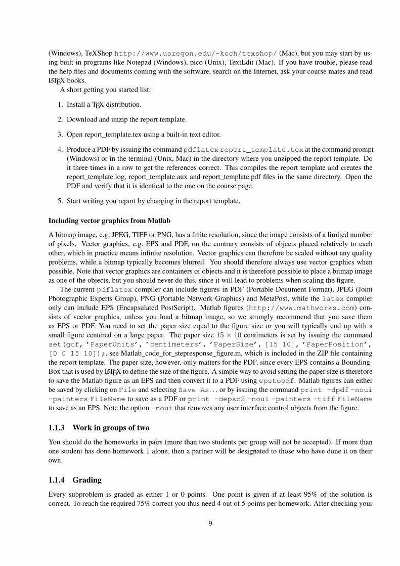
Figure 1.2: Cover and grading guide for the homeworks.
homework, we will provide a cover (see Figure 1.2) with a set of formal requirements. You need to get a passon each of the formal requirements listed on the cover and grading guide in order to pass the homework. If anyof the fail boxes is marked then you need to correct all errors and implement all improvements suggested by thereviewers or motivate why you have not implemented a suggestion. You should mark all the changes in yourPDF file (with a color that is easy to distinguish from the rest of the text; e.g., red, green, etc) and then, hand in
10

within two weeks from the day the graded homeworks were available.
1.1.5 References
[1] Tobias Oetiker, Hubert Partl, Irene Hyna, and Elisabeth Schlegl. The Not So Short Introduction to LATEX 2ε.Oetiker, OETIKER+PARTNER AG, Aarweg 15, 4600 Olten, Switzerland, 2008.http://www.ctan.org/info/lshort/.[2] Hassan K Khalil. Nonlinear systems. Prentice Hall, Upper Saddle river, 3. edition, 2002. ISBN 0-13-067389-7.
11
1.2 Homework 1
Suppose that there is a grassy island supporting populations of two species x and y. If the populations arelarge then it is reasonable to let the normalized populations be continuous functions of time (so that x = 1might represent a population of 100 000 species). We propose the following simple model of the change inpopulation:
x(t) = x(t)(a+ bx(t) + cy(t))
y(t) = y(t)(d+ ex(t) + fy(t)),(1.1)
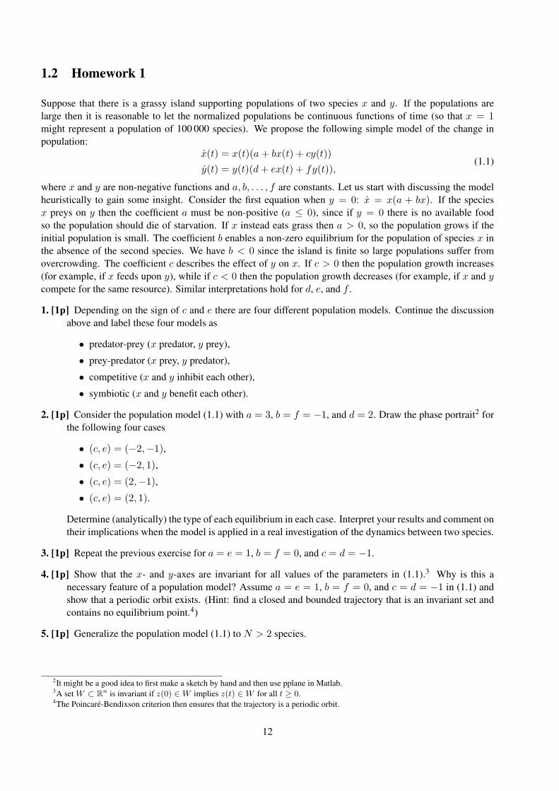
where x and y are non-negative functions and a, b, . . . , f are constants. Let us start with discussing the modelheuristically to gain some insight. Consider the first equation when y = 0: x = x(a + bx). If the speciesx preys on y then the coefficient a must be non-positive (a ≤ 0), since if y = 0 there is no available foodso the population should die of starvation. If x instead eats grass then a > 0, so the population grows if theinitial population is small. The coefficient b enables a non-zero equilibrium for the population of species x inthe absence of the second species. We have b < 0 since the island is finite so large populations suffer fromovercrowding. The coefficient c describes the effect of y on x. If c > 0 then the population growth increases(for example, if x feeds upon y), while if c < 0 then the population growth decreases (for example, if x and ycompete for the same resource). Similar interpretations hold for d, e, and f .
1. [1p] Depending on the sign of c and e there are four different population models. Continue the discussionabove and label these four models as
• predator-prey (x predator, y prey),
• prey-predator (x prey, y predator),
• competitive (x and y inhibit each other),
• symbiotic (x and y benefit each other).
2. [1p] Consider the population model (1.1) with a = 3, b = f = −1, and d = 2. Draw the phase portrait2 forthe following four cases
• (c, e) = (−2,−1),
• (c, e) = (−2, 1),
• (c, e) = (2,−1),
• (c, e) = (2, 1).
Determine (analytically) the type of each equilibrium in each case. Interpret your results and comment ontheir implications when the model is applied in a real investigation of the dynamics between two species.
3. [1p] Repeat the previous exercise for a = e = 1, b = f = 0, and c = d = −1.
4. [1p] Show that the x- and y-axes are invariant for all values of the parameters in (1.1).3 Why is this anecessary feature of a population model? Assume a = e = 1, b = f = 0, and c = d = −1 in (1.1) andshow that a periodic orbit exists. (Hint: find a closed and bounded trajectory that is an invariant set andcontains no equilibrium point.4)
5. [1p] Generalize the population model (1.1) to N > 2 species.
2It might be a good idea to first make a sketch by hand and then use pplane in Matlab.3A set W ⊂ R
n is invariant if z(0) ∈ W implies z(t) ∈ W for all t ≥ 0.4The Poincaré-Bendixson criterion then ensures that the trajectory is a periodic orbit.
12
1.3 Homework 2
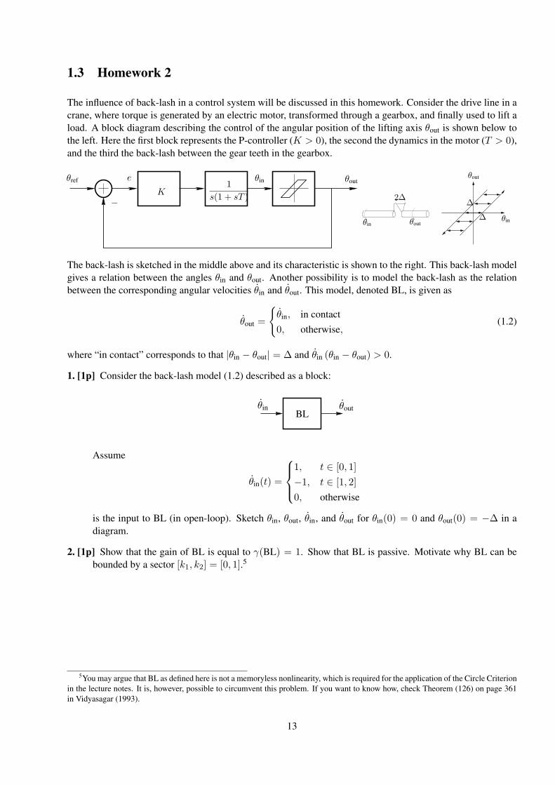
The influence of back-lash in a control system will be discussed in this homework. Consider the drive line in acrane, where torque is generated by an electric motor, transformed through a gearbox, and finally used to lift aload. A block diagram describing the control of the angular position of the lifting axis θout is shown below tothe left. Here the first block represents the P-controller (K > 0), the second the dynamics in the motor (T > 0),and the third the back-lash between the gear teeth in the gearbox.
θref
−
e θoutθin1
s(1 + sT )K
θin θout
2∆
θin
∆
∆
θout
The back-lash is sketched in the middle above and its characteristic is shown to the right. This back-lash modelgives a relation between the angles θin and θout. Another possibility is to model the back-lash as the relationbetween the corresponding angular velocities θin and θout. This model, denoted BL, is given as
θout =
θin, in contact
0, otherwise,(1.2)
where “in contact” corresponds to that |θin − θout| = ∆ and θin (θin − θout) > 0.
1. [1p] Consider the back-lash model (1.2) described as a block:
θin θoutBL
Assume
θin(t) =
1, t ∈ [0, 1]
−1, t ∈ [1, 2]
0, otherwise
is the input to BL (in open-loop). Sketch θin, θout, θin, and θout for θin(0) = 0 and θout(0) = −∆ in adiagram.
2. [1p] Show that the gain of BL is equal to γ(BL) = 1. Show that BL is passive. Motivate why BL can bebounded by a sector [k1, k2] = [0, 1].5
5You may argue that BL as defined here is not a memoryless nonlinearity, which is required for the application of the Circle Criterionin the lecture notes. It is, however, possible to circumvent this problem. If you want to know how, check Theorem (126) on page 361in Vidyasagar (1993).
13
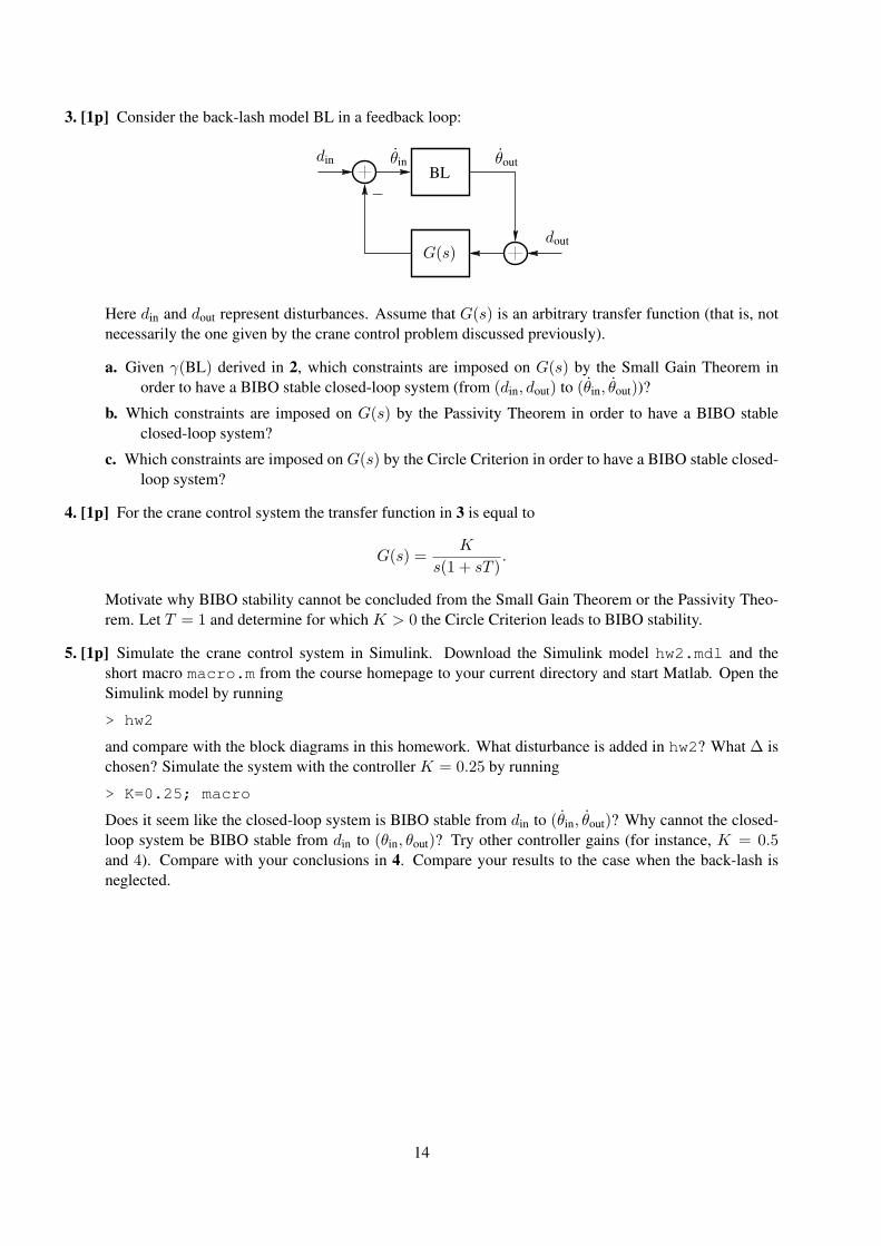
3. [1p] Consider the back-lash model BL in a feedback loop:
θin θoutdin
dout
−BL
G(s)
Here din and dout represent disturbances. Assume that G(s) is an arbitrary transfer function (that is, notnecessarily the one given by the crane control problem discussed previously).
a. Given γ(BL) derived in 2, which constraints are imposed on G(s) by the Small Gain Theorem inorder to have a BIBO stable closed-loop system (from (din, dout) to (θin, θout))?
b. Which constraints are imposed on G(s) by the Passivity Theorem in order to have a BIBO stableclosed-loop system?
c. Which constraints are imposed on G(s) by the Circle Criterion in order to have a BIBO stable closed-loop system?
4. [1p] For the crane control system the transfer function in 3 is equal to
G(s) =K
s(1 + sT ).
Motivate why BIBO stability cannot be concluded from the Small Gain Theorem or the Passivity Theo-rem. Let T = 1 and determine for which K > 0 the Circle Criterion leads to BIBO stability.
5. [1p] Simulate the crane control system in Simulink. Download the Simulink model hw2.mdl and theshort macro macro.m from the course homepage to your current directory and start Matlab. Open theSimulink model by running
> hw2
and compare with the block diagrams in this homework. What disturbance is added in hw2? What ∆ ischosen? Simulate the system with the controller K = 0.25 by running
> K=0.25; macro
Does it seem like the closed-loop system is BIBO stable from din to (θin, θout)? Why cannot the closed-loop system be BIBO stable from din to (θin, θout)? Try other controller gains (for instance, K = 0.5and 4). Compare with your conclusions in 4. Compare your results to the case when the back-lash isneglected.
14
1.4 Homework 3
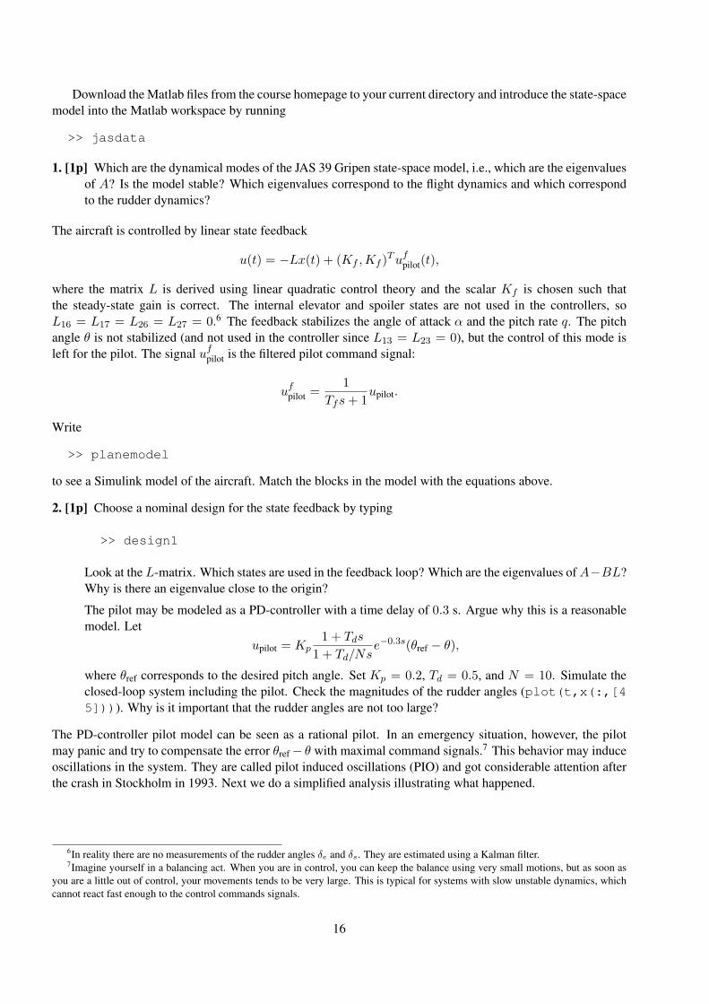
Simulation and control of the pitch angle dynamics of a JAS 39 Gripen is discussed in this homework, but firstwe give some background. The dynamics of an airplane is highly nonlinear. The control system is based ongain scheduling of speed and altitude to compensate for some of the nonlinearities. For the JAS 39 Gripen,linear models have been obtained for approximately 50 different operating conditions. The models are theresult of extensive research including wind tunnel experiments. A linear controller is designed for each linearmodel, and a switching mechanism is used to switch between the different controllers. Many of the parametersin the models vary considerably within normal operation of the aircraft. Two extreme cases are “heavily loadedaircraft at low speed” and “unloaded aircraft at high speed”. The case when the velocity of the aircraft isapproximately equal to the speed of sound is also critical, because at higher velocities the aircraft is stablewhile for lower it is unstable. The velocity of an aircraft is specified by the Mach number M = v/a, which isthe conventional velocity v normalized by the speed of sound a.
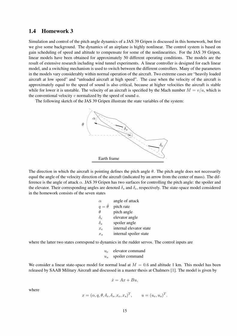
The following sketch of the JAS 39 Gripen illustrate the state variables of the system:
α
θδs
δe
Earth frame
The direction in which the aircraft is pointing defines the pitch angle θ. The pitch angle does not necessarilyequal the angle of the velocity direction of the aircraft (indicated by an arrow from the center of mass). The dif-ference is the angle of attack α. JAS 39 Gripen has two surfaces for controlling the pitch angle: the spoiler andthe elevator. Their corresponding angles are denoted δs and δe, respectively. The state-space model consideredin the homework consists of the seven states
α angle of attackq = θ pitch rateθ pitch angleδe elevator angleδs spoiler anglexe internal elevator statexs internal spoiler state
where the latter two states correspond to dynamics in the rudder servos. The control inputs are
ue elevator commandus spoiler command
We consider a linear state-space model for normal load at M = 0.6 and altitude 1 km. This model has beenreleased by SAAB Military Aircraft and discussed in a master thesis at Chalmers [1]. The model is given by
x = Ax+Bu,
wherex = (α, q, θ, δe, δs, xe, xs)
T , u = (ue, us)T .
15
Download the Matlab files from the course homepage to your current directory and introduce the state-spacemodel into the Matlab workspace by running
>> jasdata
1. [1p] Which are the dynamical modes of the JAS 39 Gripen state-space model, i.e., which are the eigenvaluesof A? Is the model stable? Which eigenvalues correspond to the flight dynamics and which correspondto the rudder dynamics?
The aircraft is controlled by linear state feedback
u(t) = −Lx(t) + (Kf ,Kf )Tufpilot(t),
where the matrix L is derived using linear quadratic control theory and the scalar Kf is chosen such thatthe steady-state gain is correct. The internal elevator and spoiler states are not used in the controllers, soL16 = L17 = L26 = L27 = 0.6 The feedback stabilizes the angle of attack α and the pitch rate q. The pitchangle θ is not stabilized (and not used in the controller since L13 = L23 = 0), but the control of this mode isleft for the pilot. The signal ufpilot is the filtered pilot command signal:
ufpilot =1
Tfs+ 1upilot.
Write
>> planemodel
to see a Simulink model of the aircraft. Match the blocks in the model with the equations above.
2. [1p] Choose a nominal design for the state feedback by typing
>> design1
Look at the L-matrix. Which states are used in the feedback loop? Which are the eigenvalues ofA−BL?Why is there an eigenvalue close to the origin?
The pilot may be modeled as a PD-controller with a time delay of 0.3 s. Argue why this is a reasonablemodel. Let
upilot = Kp1 + Tds
1 + Td/Nse−0.3s(θref − θ),
where θref corresponds to the desired pitch angle. Set Kp = 0.2, Td = 0.5, and N = 10. Simulate theclosed-loop system including the pilot. Check the magnitudes of the rudder angles (plot(t,x(:,[45]))). Why is it important that the rudder angles are not too large?
The PD-controller pilot model can be seen as a rational pilot. In an emergency situation, however, the pilotmay panic and try to compensate the error θref − θ with maximal command signals.7 This behavior may induceoscillations in the system. They are called pilot induced oscillations (PIO) and got considerable attention afterthe crash in Stockholm in 1993. Next we do a simplified analysis illustrating what happened.
6In reality there are no measurements of the rudder angles δe and δs. They are estimated using a Kalman filter.7Imagine yourself in a balancing act. When you are in control, you can keep the balance using very small motions, but as soon as
you are a little out of control, your movements tends to be very large. This is typical for systems with slow unstable dynamics, whichcannot react fast enough to the control commands signals.
16
3. [1p] In order to analyze the PIO mode, we will replace the PD-controller pilot by a relay model. The pilotthen gives maximal joystick commands based on the sign of θ. Such a “relay pilot” can be found in theSimulink pilot model library; run
>> pilotlib
Plot the Nyquist curve of the linear system from upilot to θ. This can be done by deleting the feedbackpath from θ, connecting an input and an output at appropriate places (inputs and outputs are found in thesimulink libraries), saving the system to a new file and using the linmod and nyquist commands.
Change pilot in the plane model by deleting the PD-controller pilot and inserting the “relay pilot”. Thedescribing function for a relay is
N(A) =4D
πA
What is D for the “relay pilot”? Use describing function analysis to predict amplitude and frequency ofa possible limit cycle. Simulate the system. How good is the prediction?
As you saw, the amplitude of the PIO is moderate. This is because the flight condition is high speed and highaltitude, and thus not extreme. Let us anyway discuss ways to reduce PIO.
4. [1p] Use design2 to change L and Kf to a faster design. Is the PIO amplitude decreased? Make thepilot filter faster by reducing the filter time constant to Tf = 0.03 (design3). Is the PIO amplitudedecreased? Discuss the results using the describing function method and thus plot the Nyquist curvesfrom upilot to θ. Are there any drawbacks with the design that gives smallest PIO amplitude?
5. [1p] Suggest a control strategy for reducing PIO in JAS 39 Gripen, with minimal influence on the pilotsability to manually control the plane. Analyze the performance of your strategy and compare it to theprevious two designs. It should outperform the previous ones.
Extra [0p] There are no rate limitations on the rudders in the discussed aircraft model. Rate limitations were,however, part of the problems with the JAS 39 Gripen control system. Introduce rate limitations as in thearticle [2], and investigate what happens to the limit cycle. Try to understand the idea of the (patented)nonlinear filter.
References
[1] Axelsson, L., Reglerstudier av back-up regulator för JAS 39 Gripen, MSc Thesis, CTH/SAAB Flygdivision,1992.
[2] Rundquist, L., K. Ståhl-Gunnarsson, and J. Enhagen, “Rate Limiters with Phase Compensation in JAS 39Gripen,” European Control Conference, 1997.
17

18
Chapter 2
Exercises
2.1 Nonlinear Models and Simulation
EXERCISE 1.1
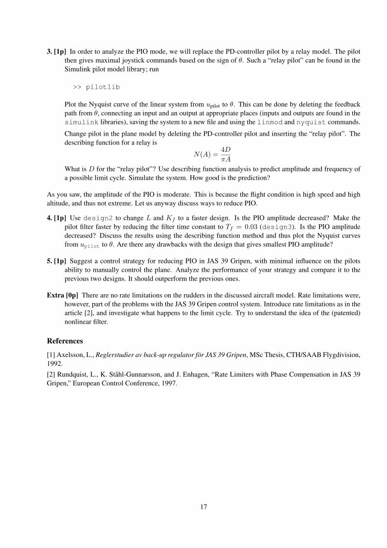
The nonlinear dynamic equation for a pendulum is given by
mlθ = −mg sin θ − klθ,
where l is the length of the pendulum, m is the mass of the bob, and θ is the angle subtended by the rod and thevertical axis through the pivot point, see Figure 1.1.
θ
Figure 2.1: The pendulum in Exercise 1.1
(a) Choose appropriate state variables and write down the state equations.
(b) Find all equilibria of the system.
(c) Linearize the system around the equilibrium points, and determine whether the system equilibria arestable or not.
19
EXERCISE 1.2
We consider a bar rotating, with friction due to viscosity, around a point where a torque is applied. The nonlinear dynamic equation of the system is given by:
ml2θ = −mgl sin(θ)− kl2θ + C
where θ is the angle between the bar and the vertical axis,C is the torque (C > 0),k is a viscous friction constant,l is the length of the barand m is the mass of the bar.
(a) Choose appropriate state variables and write down the state equations.
(b) Find all equilibria of the system, assuming that Cmlg < 1.
(c) Linearize the system around the equilibrium points and determine the eigenvalues for each equilibrium.
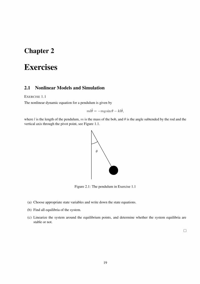
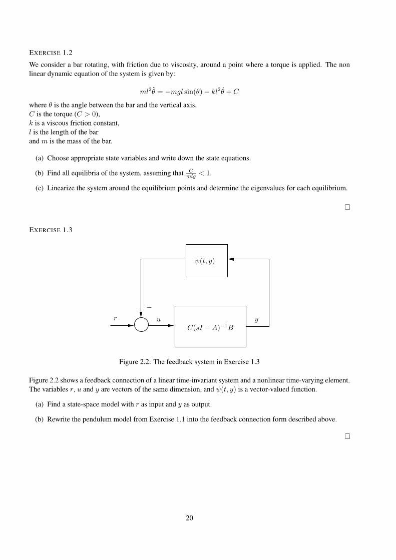
EXERCISE 1.3
r
−u
ψ(t, y)
yC(sI −A)−1B
Figure 2.2: The feedback system in Exercise 1.3
Figure 2.2 shows a feedback connection of a linear time-invariant system and a nonlinear time-varying element.The variables r, u and y are vectors of the same dimension, and ψ(t, y) is a vector-valued function.
(a) Find a state-space model with r as input and y as output.
(b) Rewrite the pendulum model from Exercise 1.1 into the feedback connection form described above.
20
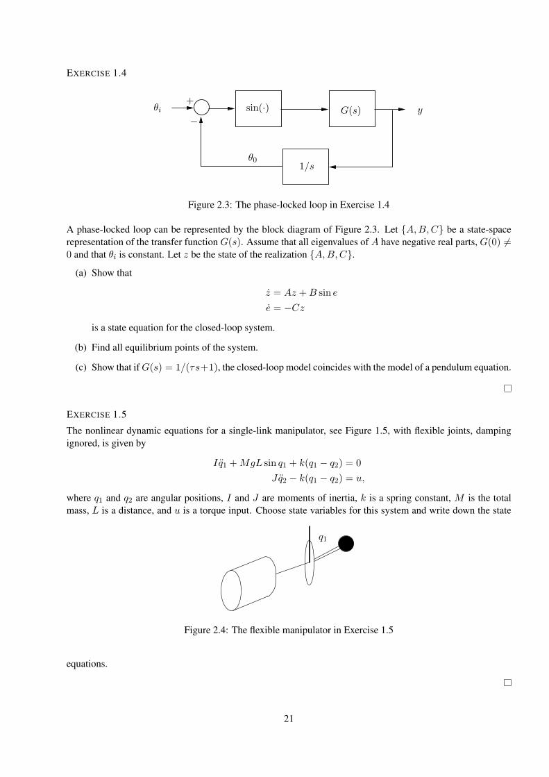
EXERCISE 1.4
−
+sin(·) G(s) y
θ0
θi
1/s
Figure 2.3: The phase-locked loop in Exercise 1.4
A phase-locked loop can be represented by the block diagram of Figure 2.3. Let A,B,C be a state-spacerepresentation of the transfer function G(s). Assume that all eigenvalues of A have negative real parts, G(0) 6=0 and that θi is constant. Let z be the state of the realization A,B,C.
(a) Show that
z = Az +B sin e
e = −Cz
is a state equation for the closed-loop system.
(b) Find all equilibrium points of the system.
(c) Show that ifG(s) = 1/(τs+1), the closed-loop model coincides with the model of a pendulum equation.
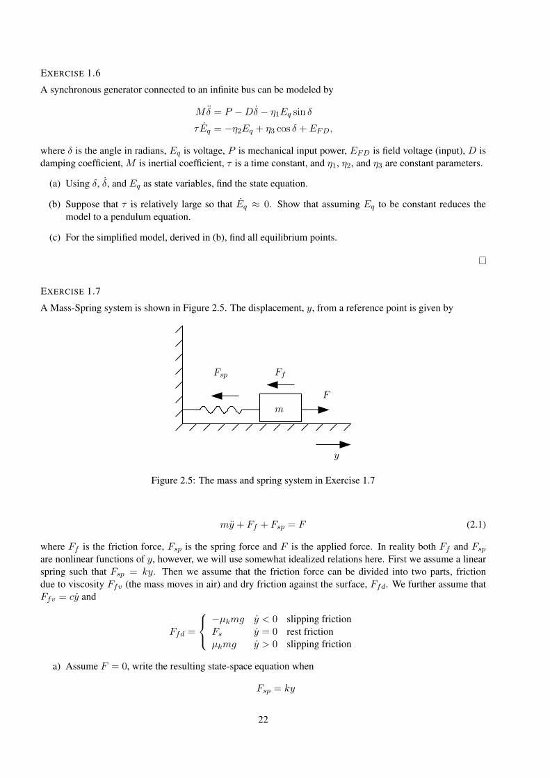
EXERCISE 1.5
The nonlinear dynamic equations for a single-link manipulator, see Figure 1.5, with flexible joints, dampingignored, is given by
Iq1 +MgL sin q1 + k(q1 − q2) = 0
Jq2 − k(q1 − q2) = u,
where q1 and q2 are angular positions, I and J are moments of inertia, k is a spring constant, M is the totalmass, L is a distance, and u is a torque input. Choose state variables for this system and write down the state
q1
Figure 2.4: The flexible manipulator in Exercise 1.5
equations.
21
EXERCISE 1.6
A synchronous generator connected to an infinite bus can be modeled by
Mδ = P −Dδ − η1Eq sin δ
τEq = −η2Eq + η3 cos δ + EFD,
where δ is the angle in radians, Eq is voltage, P is mechanical input power, EFD is field voltage (input), D isdamping coefficient, M is inertial coefficient, τ is a time constant, and η1, η2, and η3 are constant parameters.
(a) Using δ, δ, and Eq as state variables, find the state equation.
(b) Suppose that τ is relatively large so that Eq ≈ 0. Show that assuming Eq to be constant reduces themodel to a pendulum equation.
(c) For the simplified model, derived in (b), find all equilibrium points.
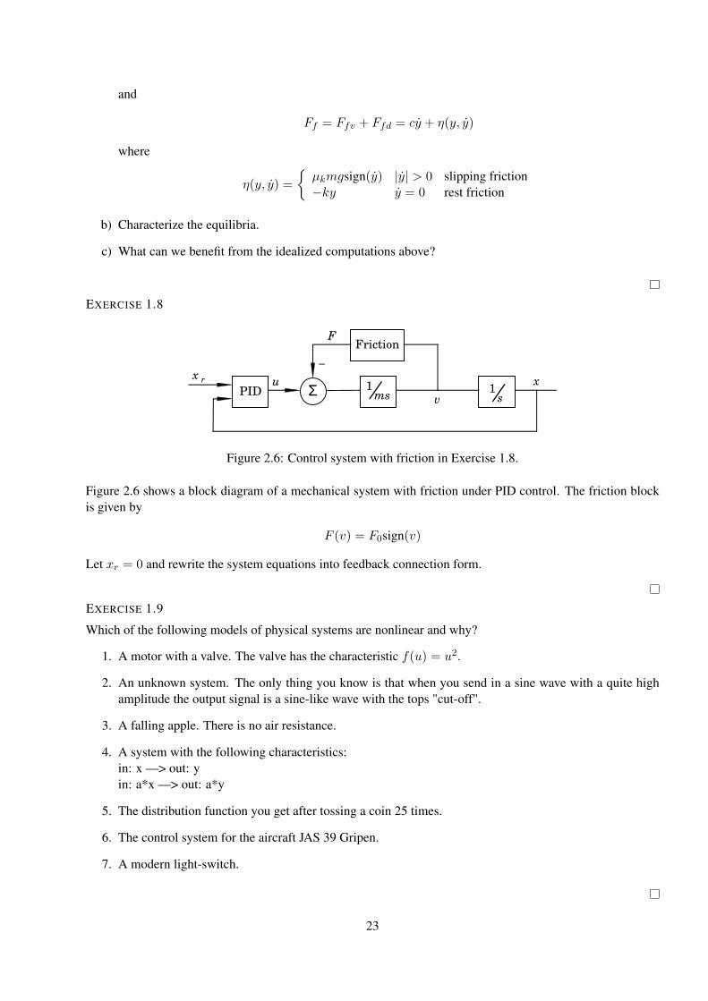
EXERCISE 1.7
A Mass-Spring system is shown in Figure 2.5. The displacement, y, from a reference point is given by
Fsp Ff
F
m
y
Figure 2.5: The mass and spring system in Exercise 1.7
my + Ff + Fsp = F (2.1)
where Ff is the friction force, Fsp is the spring force and F is the applied force. In reality both Ff and Fsp
are nonlinear functions of y, however, we will use somewhat idealized relations here. First we assume a linearspring such that Fsp = ky. Then we assume that the friction force can be divided into two parts, frictiondue to viscosity Ffv (the mass moves in air) and dry friction against the surface, Ffd. We further assume thatFfv = cy and
Ffd =
−µkmg y < 0 slipping frictionFs y = 0 rest frictionµkmg y > 0 slipping friction
a) Assume F = 0, write the resulting state-space equation when
Fsp = ky
22
and
Ff = Ffv + Ffd = cy + η(y, y)
where
η(y, y) =
µkmgsign(y) |y| > 0 slipping friction−ky y = 0 rest friction
b) Characterize the equilibria.
c) What can we benefit from the idealized computations above?
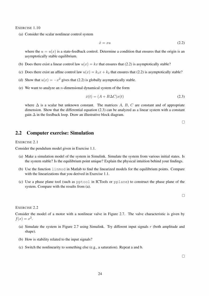
EXERCISE 1.8
Friction
ux r
v
x
F
1s
ΣPID1
ms
−
Figure 2.6: Control system with friction in Exercise 1.8.
Figure 2.6 shows a block diagram of a mechanical system with friction under PID control. The friction blockis given by
F (v) = F0sign(v)
Let xr = 0 and rewrite the system equations into feedback connection form.
EXERCISE 1.9
Which of the following models of physical systems are nonlinear and why?
1. A motor with a valve. The valve has the characteristic f(u) = u2.
2. An unknown system. The only thing you know is that when you send in a sine wave with a quite highamplitude the output signal is a sine-like wave with the tops "cut-off".
3. A falling apple. There is no air resistance.
4. A system with the following characteristics:in: x —> out: yin: a*x —> out: a*y
5. The distribution function you get after tossing a coin 25 times.
6. The control system for the aircraft JAS 39 Gripen.
7. A modern light-switch.
23
EXERCISE 1.10
(a) Consider the scalar nonlinear control system
x = xu (2.2)
where the u = u(x) is a state-feedback control. Determine a condition that ensures that the origin is anasymptotically stable equilibrium.
(b) Does there exist a linear control law u(x) = kx that ensures that (2.2) is asymptotically stable?
(c) Does there exist an affine control law u(x) = k1x+ k2 that ensures that (2.2) is asymptotically stable?
(d) Show that u(x) = −x2 gives that (2.2) is globally asymptotically stable.
(e) We want to analyze an n-dimensional dynamical system of the form
x(t) = (A+B∆C)x(t) (2.3)
where ∆ is a scalar but unknown constant. The matrices A, B, C are constant and of appropriatedimension. Show that the differential equation (2.3) can be analyzed as a linear system with a constantgain ∆ in the feedback loop. Draw an illustrative block diagram.
2.2 Computer exercise: Simulation
EXERCISE 2.1
Consider the pendulum model given in Exercise 1.1.
(a) Make a simulation model of the system in Simulink. Simulate the system from various initial states. Isthe system stable? Is the equilibrium point unique? Explain the physical intuition behind your findings.
(b) Use the function linmod in Matlab to find the linearized models for the equilibrium points. Comparewith the linearizations that you derived in Exercise 1.1.
(c) Use a phase plane tool (such as pptool in ICTools or pplane) to construct the phase plane of thesystem. Compare with the results from (a).
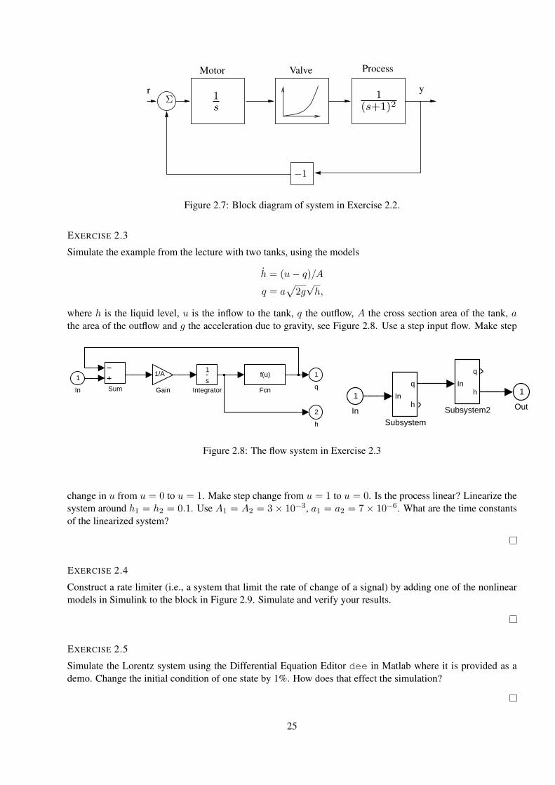
EXERCISE 2.2
Consider the model of a motor with a nonlinear valve in Figure 2.7. The valve characteristic is given byf(x) = x2.
(a) Simulate the system in Figure 2.7 using Simulink. Try different input signals r (both amplitude andshape).
(b) How is stability related to the input signals?
(c) Switch the nonlinearity to something else (e.g., a saturation). Repeat a and b.
24
PSfrag
Σ 1s
1(s+1)2
Motor Valve Process
−1
r y
Figure 2.7: Block diagram of system in Exercise 2.2.
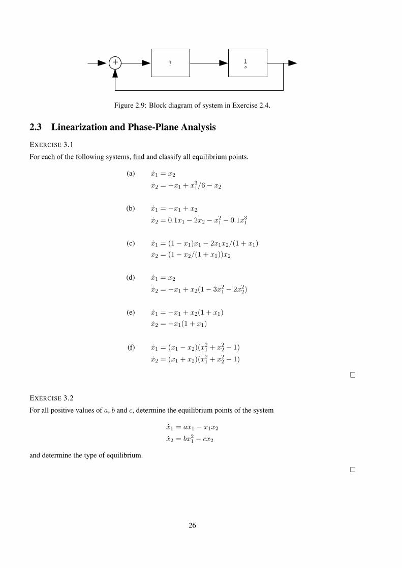
EXERCISE 2.3
Simulate the example from the lecture with two tanks, using the models
h = (u− q)/A
q = a√2g
√h,
where h is the liquid level, u is the inflow to the tank, q the outflow, A the cross section area of the tank, athe area of the outflow and g the acceleration due to gravity, see Figure 2.8. Use a step input flow. Make step
2
h
1
qSums
1
Integrator
1/A
Gain
f(u)
Fcn
1
In 1
Out
In
q
h
Subsystem2
In
q
h
Subsystem
1
In
Figure 2.8: The flow system in Exercise 2.3
change in u from u = 0 to u = 1. Make step change from u = 1 to u = 0. Is the process linear? Linearize thesystem around h1 = h2 = 0.1. Use A1 = A2 = 3× 10⁻³, a1 = a2 = 7× 10⁻⁶. What are the time constantsof the linearized system?
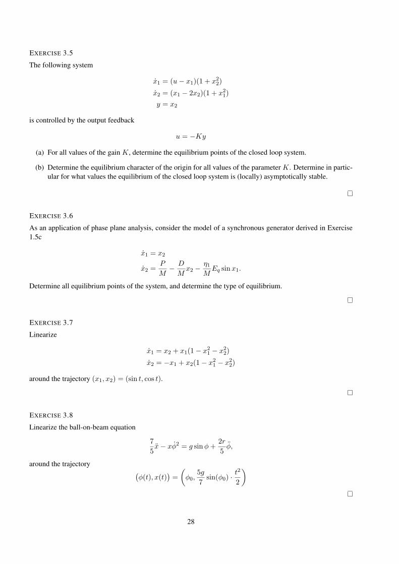
EXERCISE 2.4
Construct a rate limiter (i.e., a system that limit the rate of change of a signal) by adding one of the nonlinearmodels in Simulink to the block in Figure 2.9. Simulate and verify your results.
EXERCISE 2.5
Simulate the Lorentz system using the Differential Equation Editor dee in Matlab where it is provided as ademo. Change the initial condition of one state by 1%. How does that effect the simulation?
25
+ 1s?
Figure 2.9: Block diagram of system in Exercise 2.4.
2.3 Linearization and Phase-Plane Analysis
EXERCISE 3.1
For each of the following systems, find and classify all equilibrium points.
(a) x1 = x2
x2 = −x1 + x31/6− x2
(b) x1 = −x1 + x2
x2 = 0.1x1 − 2x2 − x21 − 0.1x31
(c) x1 = (1− x1)x1 − 2x1x2/(1 + x1)
x2 = (1− x2/(1 + x1))x2
(d) x1 = x2
x2 = −x1 + x2(1− 3x21 − 2x22)
(e) x1 = −x1 + x2(1 + x1)
x2 = −x1(1 + x1)
(f) x1 = (x1 − x2)(x21 + x22 − 1)
x2 = (x1 + x2)(x21 + x22 − 1)
EXERCISE 3.2
For all positive values of a, b and c, determine the equilibrium points of the system
x1 = ax1 − x1x2
x2 = bx21 − cx2
and determine the type of equilibrium.
26
EXERCISE 3.3
For each of the following systems, construct the phase portrait, preferably using a computer program, anddiscuss the qualitative behaviour of the system.
(a) x1 = x2
x2 = x1 − 2 tan−1(x1 + x2)
(b) x1 = x2
x2 = −x1 + x2(1− 3x21 − 2x22)
(c) x1 = 2x1 − x1x2
x2 = 2x21 − x2
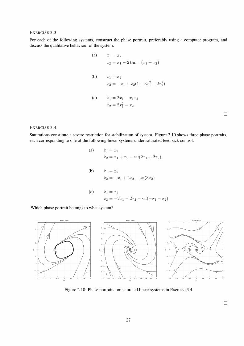
EXERCISE 3.4
Saturations constitute a severe restriction for stabilization of system. Figure 2.10 shows three phase portraits,each corresponding to one of the following linear systems under saturated feedback control.
(a) x1 = x2
x2 = x1 + x2 − sat(2x1 + 2x2)
(b) x1 = x2
x2 = −x1 + 2x2 − sat(3x2)
(c) x1 = x2
x2 = −2x1 − 2x2 − sat(−x1 − x2)
Which phase portrait belongs to what system?
−2 −1.5 −1 −0.5 0 0.5 1 1.5 2−2
−1.5
−1
−0.5
0
0.5
1
1.5
2
x1
x2
Phase plane
−1 −0.8 −0.6 −0.4 −0.2 0 0.2 0.4 0.6 0.8 1−1
−0.8
−0.6
−0.4
−0.2
0
0.2
0.4
0.6
0.8
1
x1
x2
Phase plane
−2 −1.5 −1 −0.5 0 0.5 1 1.5 2
−1.5
−1
−0.5
0
0.5
1
1.5
2
x1
x2
Phase plane
Figure 2.10: Phase portraits for saturated linear systems in Exercise 3.4
27
EXERCISE 3.5
The following system
x1 = (u− x1)(1 + x22)
x2 = (x1 − 2x2)(1 + x21)
y = x2
is controlled by the output feedback
u = −Ky
(a) For all values of the gain K, determine the equilibrium points of the closed loop system.
(b) Determine the equilibrium character of the origin for all values of the parameter K. Determine in partic-ular for what values the equilibrium of the closed loop system is (locally) asymptotically stable.
EXERCISE 3.6
As an application of phase plane analysis, consider the model of a synchronous generator derived in Exercise1.5c
x1 = x2
x2 =P
M− D
Mx2 −
η1MEq sinx1.
Determine all equilibrium points of the system, and determine the type of equilibrium.
EXERCISE 3.7
Linearize
x1 = x2 + x1(1− x21 − x22)
x2 = −x1 + x2(1− x21 − x22)
around the trajectory (x1, x2) = (sin t, cos t).
EXERCISE 3.8
Linearize the ball-on-beam equation
7
5x− xφ2 = g sinφ+
2r
5φ,
around the trajectory(φ(t), x(t)
)=
(φ0,
5g
7sin(φ0) ·
t2
2
)
28
EXERCISE 3.9
Use a simple trigonometry identity to help find a nominal solution corresponding to u(t) = sin (3t), y(0) =0, y(0) = 1 for the eqution
y +4
3y3(t) = −1
3u(t).
Linearize the equation around this nominal solution.
EXERCISE 3.10
A regular bicycle is mainly controlled by turning the handle bars.1 Let the tilt sideways of the bicycle be θradians and the turning angle of the front wheel be β radians. The tilt of the bike obeys the following nonlineardifferential equation:
θ =mgℓ
Jsin θ +
mℓV 20
bJcos θ tanβ +
amℓV0bJ
· cos θ
cos2 βu
β = u,
where V0 > 0 is the (constant) velocity of the bicycle, and m, g, ℓ, J , a, and b are other positive constants.The control u is the angular velocity applied at the handle bars. To gain some understanding of the principalbehavior of the bicycle, we study its linearization. Linearize the tilt equation around the equilibrium point(θ, β, u) = (0, 0, 0).
Derive the transfer function G(s) from u to θ. Determine the poles and zeros of G(s). Is the bike locallystable?
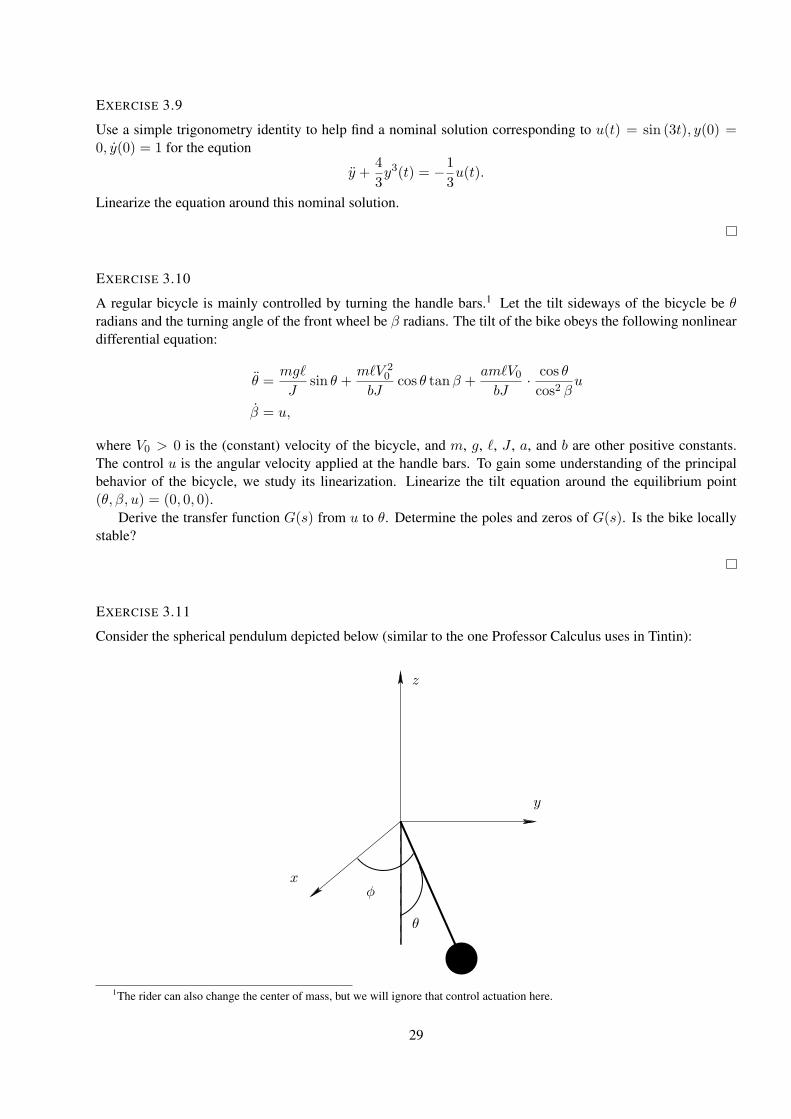
EXERCISE 3.11
Consider the spherical pendulum depicted below (similar to the one Professor Calculus uses in Tintin):
x
y
z
φ
θ
1The rider can also change the center of mass, but we will ignore that control actuation here.
29
Here θ denotes the angular position of the pendulum with respect to the z-axis and φ denotes the angularposition in the x-y plane. A (normalized) model of the spherical pendulum is given by
θ − φ2 sin θ cos θ + sin θ = 0
φ sin θ + 2φθ cos θ = 0
(a) Specify the pendulum dynamics on first-order form
x = f(x)
and give condition on when the first-order form is equivalent to the original equations.
(b) Determine all equilibria for the pendulum system. (You don’t have to determine stability properties.)[Hint: Consider the original equations.]
(c) Show that (θ(t), φ(t)) = (π/3, t√2) is a trajectory of the pendulum system.
(d) Linearize the pendulum system about the trajectory in (c).
2.4 Lyapunov Stability
EXERCISE 4.1
Consider the scalar system
x = ax3
(a) Show that Lyapunov’s linearization method fails to determine stability of the origin.
(b) Use the Lyapunov function
V (x) = x4
to show that the system is stable for a < 0 and unstable for a > 0.
(c) What can you say about the system for a = 0?
EXERCISE 4.2
Consider the pendulum equation
x1 = x2
x2 = −glsinx1 −
k
lx2.
(a) Assume zero friction, i.e. let k = 0, and show that the origin is stable. (Hint. Show that the energy of thependulum is constant along all system trajectories.)
(b) Can the pendulum energy be used to show asymptotic stability for the pendulum with non-zero friction,k 6= 0? If not, modify the Lyapunov function to show asymptotic stability of the origin.
30
EXERCISE 4.3
Consider the system
x+ dx3 + kx = 0.
Show that
V (x) =1
2
(kx2 + x2
)
is a Lyapunov function. Is the system locally stable, locally asymptotically stable, and globally asymptoticallystable?
EXERCISE 4.4
Consider the linear system
x = Ax =
[0 −11 −1
]x
(a) Compute the eigenvalues of A and verify that the system is asymptotically stable
(b) From the lectures, we know that an equivalent characterization of stability can be obtained by consideringthe Lyapunov equation
ATP + PA = −Q
where Q = QT is any positive definite matrix. The system is asymptotically stable if and only if thesolution P to the Lyapunov equation is positive definite.
(i) Let
P =
[p11 p12p12 p22
]
Verify by completing squares that V (x) = xTPx is a positive definite function if and only if
p11 > 0, p11p22 − p212 > 0
(ii) Solve the Lyapunov function with Q as the identity matrix. Is the solution P a positive definitematrix?
(c) Solve the Lyapunov equation in Matlab.
EXERCISE 4.5
As you know, the systemx(t) = Ax(t), t ≥ 0,
is asymptotically stable if all eigenvalues of A have negative real parts. It might be tempted to conjecture thatthe time-varying system
x(t) = A(t)x(t), t ≥ 0, (2.4)
is asymptotically stable if the eigenvalues of A(t) have negative real parts for all t ≥ 0. This is not true.
31
(a) Show this by explicitly deriving the solution of
x =
[−1 e2t
0 −1
]x, t ≥ 0.
(b) The system (2.4) is however stable if the eigenvalues of A(t) + AT (t) have negative real parts for allt ≥ 0. Prove this by showing that V = xTx is a Lyapunov function.
EXERCISE 4.6
A student is confronted with the nonlinear differential equation
x+2x
(1 + x2)2= 0
and is asked to determine whether or not the equation is stable. The students think “this is an undamped mass-spring system – the spring is nonlinear with a spring constant of 2/(1+x2)2”. The student re-writes the systemas
x1 = x2
x2 =−2x1
(1 + x21)2
and constructs the obvious Lyapunov function
V (x) =
∫ x1
0
2ζ
(1 + ζ2)2dζ +
1
2x22.
The student declares, “V is positive definite, because everywhere in IR2, V (x) ≥ 0, and V (x) = 0 only ifx = 0.” The student ascertains that V ≤ 0 everywhere in IR2 and concludes, “the conditions for Lyapunov’stheorem are satisfied, so the system is globally stable about x = 0”.
(a) Sadly, there is a mistake in the student’s reasoning. What is the mistake?
(b) Perhaps the student has merely made a poor choice of Lyapunov function, and the system really isglobally asymptotically stable. Is there some other Lyapunov function that can be used to show globalstability? Find such a function, or show that no such function exists.
EXERCISE 4.7
Consider the system
x1 = x2 − x71(x41 + 2x22 − 10
)
x2 = −x31 − 3x52(x41 + 2x22 − 10
) (2.5)
(a) For which values of C is the setx ∈ R2|x41 + 2x22 ≤ C
invariant with respect to (2.5)?
(b) Use LaSalle’s invariant set theorem to analyze the behavior of the system. (Hint: Use V (x) = (x41 +2x22 − 10)2).
32
(c) Repeat (a) and (b), but now with the setx ∈ R2|ǫ ≤ x41 + 2x22 ≤ C
. What can be said about the
stability of the origin?
EXERCISE 4.8
Consider the system
x1 = x2
x2 = −2x1 − 2x2 − 4x31
Use the function
V (x) = 4x21 + 2x22 + 4x41
to show that
(a) the system is globally stable around the origin.
(b) the origin is globally asymptotically stable.
EXERCISE 4.9
Consider the system
x1 = x2
x2 = x1 − sat(2x1 + x2).
(a) Show that the origin is asymptotically stable.
(b) Show that all trajectories starting in the first quadrant to the right of the curve
x1x2 = c
for sufficiently large c, cannot reach the origin. (Hint: Consider V (x) = x1x2; calculate V (x) and showthat on the curve V (x) = c, the derivative V (x) > 0 when c is sufficiently large.)
(c) Show that the origin is not globally asymptotically stable.
EXERCISE 4.10
In general, it is non-trivial to find a Lyapunov function for a given nonlinear system. Several different methodshave been derived for specific classes of systems. In this exercise, we will investigate the following method,known as Krasovskii’s method.
Consider systems on the form
x = f(x)
with f(0) = 0. Assume that f(x) is continuously differentiable and that its Jacobian, ∂f/∂x, satisfies
P∂f
∂x(x) +
(∂f
∂x(x)
)T
P ≤ −I
for all x ∈ IRn, and some matrix P = P T > 0. Then, the origin is globally asymptotically stable withV (x) = fT (x)Pf(x) as Lyapunov function.
Prove the validity of the method in the following steps.
33
(a) Verify that f(x) can be written as
f(x) =
∫ 1
0
∂f
∂x(σx) · x dσ.
and use this representation to show that the assumptions imply
xTPf(x) + fT (x)Px ≤ −xTx, ∀x ∈ IRn
(b) Show that V (x) = fT (x)Pf(x) is positive definite for all x ∈ IRn.
(c) Show that V (x) is radially unbounded.
(d) Using V (x) as a Lyapunov function candidate, show that the origin is globally asymptotically stable.
2.5 Input-Output Stability
EXERCISE 5.1
The norms used in the definitions of stability need not be the usual Euclidian norm. If the state-space is of finitedimension n (i.e., the state vector has n components), stability and its type are independent of the choice ofnorm (all norms are “equivalent”), although a particular choice of norm may make analysis easier. For n = 2,draw the unit balls corresponding to the following norms.
(a) ||x||2 = x21 + x22 (Euclidian norm)
(b) ||x||2 = x21 + 5x22
(c) ||x|| = |x1|+ |x2|
(d) ||x|| = sup(|x1|, |x2|)
Recall that a “ball” B(x0, R), of center x0 and radius R, is the set of x such that ||x − x0|| ≤ R, and that theunit ball is B(0, 1).
EXERCISE 5.2
Compute the norms ‖ · ‖∞ and ‖ · ‖2 for the signals
(a)
y(t) =
a sin(t) t > 00 t ≤ 0
(b)
y(t) =
1t t > 10 t ≤ 1
(c)
y(t) =
e−t(1− e−t) t > 00 t ≤ 0
34
EXERCISE 5.3
Consider the linear system
G(s) =ω20
s2 + 2ζω0s+ ω20
.
Compute the gain of ‖G‖ for all ω0 > 0 and ζ > 0.
EXERCISE 5.4
Consider a linear time invariant system G(s) interconnected with a static nonlinearity ψ(y) in the standardform. Compare the Nyquist, Small Gain, Circle Criterion and Passivity theorem with respect to the followingissues.
(a) What are the restrictions that must be imposed on ψ(y) in order to apply the different stability criteria?
(b) What restrictions must be imposed on the Nyquist curve of the linear system in order to apply the stabilitycriteria above?
EXERCISE 5.5
−2 −1.5 −1 −0.5 0 0.5 1 1.5 2−1.5
−1
−0.5
0
0.5
1
1.5
−2 −1.5 −1 −0.5 0 0.5 1 1.5 2−1.5
−1
−0.5
0
0.5
1
1.5
−2 −1.5 −1 −0.5 0 0.5 1 1.5 2−1.5
−1
−0.5
0
0.5
1
1.5
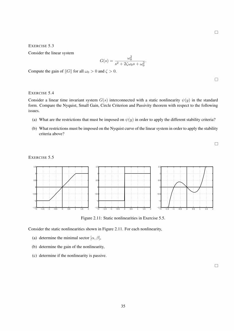
Figure 2.11: Static nonlinearities in Exercise 5.5.
Consider the static nonlinearities shown in Figure 2.11. For each nonlinearity,
(a) determine the minimal sector [α, β],
(b) determine the gain of the nonlinearity,
(c) determine if the nonlinearity is passive.
35
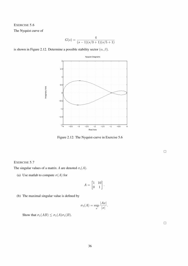
EXERCISE 5.6
The Nyquist curve of
G(s) =4
(s− 1)(s/3 + 1)(s/5 + 1)
is shown in Figure 2.12. Determine a possible stability sector (α, β).
Real Axis
Imag
inar
y A
xis
Nyquist Diagrams
−4 −3.5 −3 −2.5 −2 −1.5 −1 −0.5 0−2
−1.5
−1
−0.5
0
0.5
1
1.5
2
Figure 2.12: The Nyquist-curve in Exercise 5.6
EXERCISE 5.7
The singular values of a matrix A are denoted σi(A).
(a) Use matlab to compute σ(A) for
A =
[1 100 1
].
(b) The maximal singular value is defined by
σ1(A) = supx
|Ax||x| .
Show that σ1(AB) ≤ σ1(A)σ1(B).
36
EXERCISE 5.8
In the previous chapter, we have seen how we can use Lyapunov functions to prove stability of systems. In thisexercise, we shall see how another type of auxillary functions, called storage functions, can be used to assesspassivity of a system.
Consider the linear system
x = Ax+Bu
y = Cx (2.6)
with zero initial conditions, x(0) = 0.
(a) Show that if we can find a storage function V (x, u) with the following properties
– V (x, u) is continuously differentiable.
– V (0) = 0 and V (x, u) ≥ 0 for x 6= 0.
– uT y ≥ V (x, u).
then, the system (2.6) is passive.
(b) Show that
V (x) =1
2xTPx
is OK as a storage function where
P :
ATP + PA = −QBTP = C
and P and Q are symmetric positive definite matrices.
EXERCISE 5.9
Let P be the solution toATP + PA = −I,
where A is a asymptotically stable matrix. Show that G(s) = BTP (sI − A)−1B is passive. (Hint. Use thefunction V (x) = xTPx.)
EXERCISE 5.10
A DC motor is characterized by
θ = ω
ω = −ω + η,
where θ is the shaft angle and η is the input voltage. The dynamic controller
z = 2(θ − z)− sat(θ − z)
η = z − 2θ
is used to control the shaft position. Use any method you like to prove that θ(t) and ω(t) converge to zero ast→ ∞.
37
EXERCISE 5.11
(a) Let uc(t) be an arbitrary function of time and let H(·) be a passive system. Show that
y(t) = uc(t) ·H(uc(t)u(t))
is passive from u to y.
(b) Show that the following adaptive system is stable
e(t) = G(s)(θ(t)− θ0
)uc(t)
θ(t) = −γuc(t)e(t),
if γ > 0 and G(s) is strictly passive.
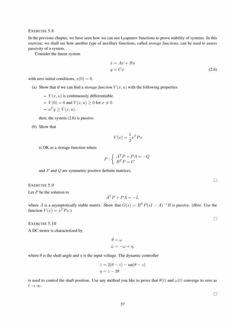
EXERCISE 5.12
(a) Consider the feedback system below with
G(s) =∆
s(s+ 1)
andf(y) = K arctan(y)
−
r yG(s)
f(·)
For what values of the uncertain (but constant) parameters ∆ > 0 and K > 0 does BIBO stability for thefeedback system follow from the Circle Criterion?
(b) For which values of ∆ > 0 and K > 0 does the direct application of the Small Gain Theorem prove BIBOstability for the feedback system in (b)? (Hint: Is the Small Gain Theorem applicable?)
EXERCISE 5.13
Consider a second-order differential equation
x = f(x),
where f : R2 → R2 is a C
1 (continuously differentiable) function such that f(0) = 0.Determine if the following statements are true or false. You have to motivate your answers to get credits.
The motivation can for example be a short proof, a counter example (Swedish: motexempel), or a reference toa result in the lecture notes.
38
(a) Suppose the differential equation (5.13) has more than one equilibria, then none of them can be globallyasymptotically stable.
(b) The differential equation (5.13) cannot have a periodic solution.
(c) If the eigenvalues of∂f
∂x(0)
are strictly in the left half-plane, then the nonlinear system (5.13) is asymptotically stable.
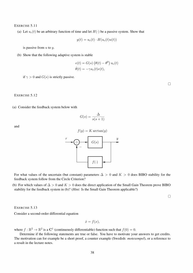
(d) There exists f such that the differential equation (5.13) have a phase portrait that looks like this:
−1 −0.8 −0.6 −0.4 −0.2 0 0.2 0.4 0.6 0.8 1−1
−0.8
−0.6
−0.4
−0.2
0
0.2
0.4
0.6
0.8
1
(e) For any initial condition x(0) = x0 6= 0, the solution x(t) of (5.13) cannot reach x = 0 in finite time,that is, there does not exist 0 < T < ∞ such that x(T ) = 0. [Hint: Since f is C1, both the equations
x = f(x) and x = −f(x) have unique solutions. What about a solution ending (for x = f(x)) and
starting (for x = −f(x)) in x0 = 0?]
39
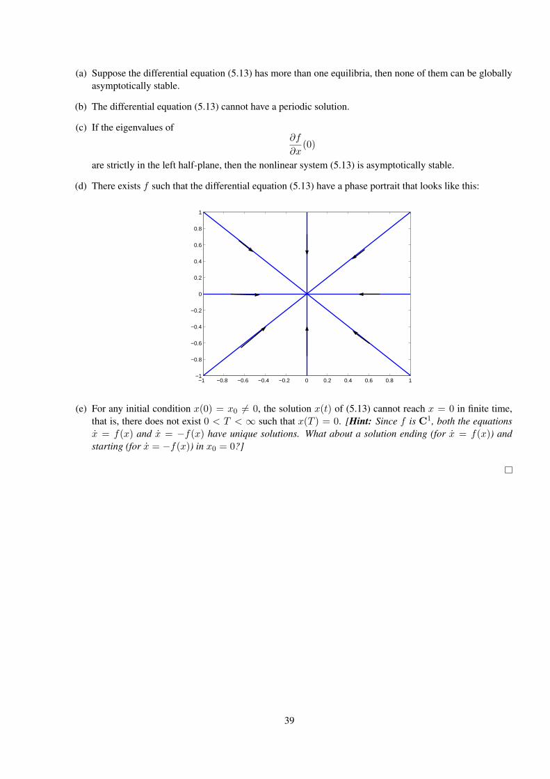
EXERCISE 5.14
We wish to estimate the domain of attraction D of the origin for the system
x1 = −x2x2 = x1 + (x21 − 1)x2,
see phase portrait below:
singlesolution
phaseportrait stop clear
axeszoom
inzoomout
solverprefs
−4 −3 −2 −1 0 1 2 3 4−4
−3
−2
−1
0
1
2
3
4
x1
x2
Phase plane
(a) Show that the origin is a locally asymptotically stable equilibrium. Linearize the system at the origin anddetermine the system matrix A.
(b) Find a Lyapunov function of the form V (x) = xTPx by solving the Lyapunov equation
PA+ATP = −2I,
for an unknown positive definite symmetric matrix P , where A is the matrix in (a).
(c) We want to find an as large region Π ⊂ R2 as possible such that for all x ∈ Π,
V =dV
dx· dxdt
< 0.
Show thatV = −2x21 − 2x22 − 2x31x2 + 4x21x
22.
40
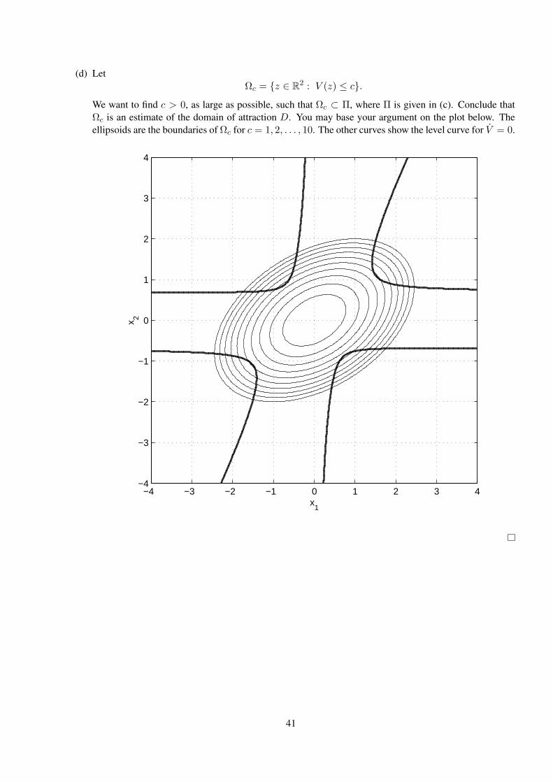
(d) LetΩc = z ∈ R
2 : V (z) ≤ c.We want to find c > 0, as large as possible, such that Ωc ⊂ Π, where Π is given in (c). Conclude thatΩc is an estimate of the domain of attraction D. You may base your argument on the plot below. Theellipsoids are the boundaries of Ωc for c = 1, 2, . . . , 10. The other curves show the level curve for V = 0.
−4 −3 −2 −1 0 1 2 3 4−4
−3
−2
−1
0
1
2
3
4
x1
x 2
41

EXERCISE 5.15
Figure 2.13: System model used in exercise
The system considered in the following tasks, contains of a linear part G(s) connected with a staticalfeedback-loop f(:) as seen in Figure 2.13.
Which statements are true, and which are false ?If false, then justify why it is so ?
1. The system is BIBO-stable if the small gain theorem shows stability for the system.
2. The system is unstable if Small Gain theorem, Circle Criteria and Passivity theorem are proved not stable.
3. The system is BIBO-stable if the Circle criteria proves BIBO-stability, even if the Small gain theorem,and Passivity theorem don’t fulfill it’s requrement for BIBO-stability.
4. If G(s) is passive and f(:) is passive, the system is BIBO-stable.
5. For the system to be strictly passive, the nyquist curve for G(iω) has to lie in the R.H.P and not intersectthe ℑ-axis, for all ω.
6. Using the Circle criteria: If the nyquist curve ofG(iω) stays inside the circle defined by the points −1/k1and −1/k2, the system is stable.k1 ≤ f(y)
y ≤ k2
42
2.6 Describing Function Analysis
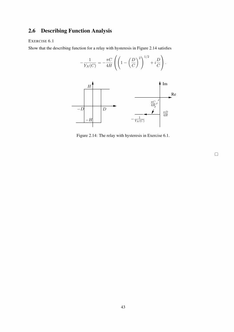
EXERCISE 6.1
Show that the describing function for a relay with hysteresis in Figure 2.14 satisfies
− 1
YN (C)= −πC
4H
(1−
(D
C
)2)1/2
+ iD
C
.
D−D
H
−H
πD4H
πC4H
− 1YN (C)
Re
Im
Figure 2.14: The relay with hysteresis in Exercise 6.1.
43
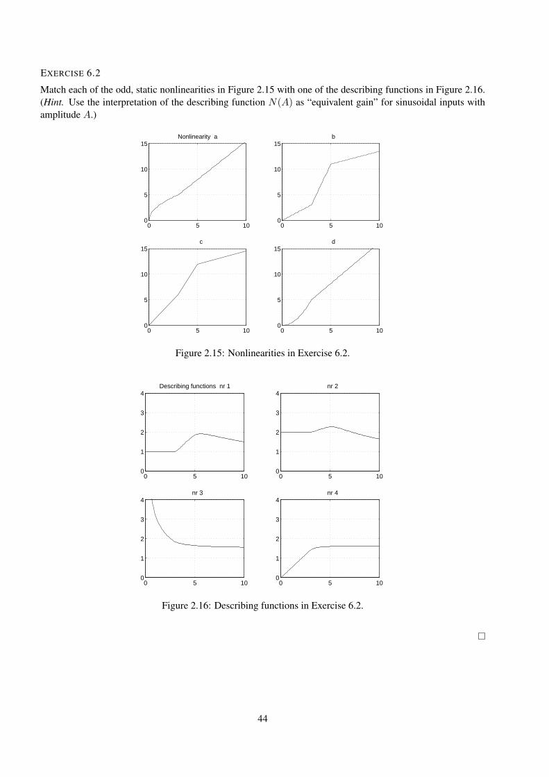
EXERCISE 6.2
Match each of the odd, static nonlinearities in Figure 2.15 with one of the describing functions in Figure 2.16.(Hint. Use the interpretation of the describing function N(A) as “equivalent gain” for sinusoidal inputs withamplitude A.)
0 5 100
5
10
15Nonlinearity a
0 5 100
5
10
15 b
0 5 100
5
10
15 d
0 5 100
5
10
15 c
Figure 2.15: Nonlinearities in Exercise 6.2.
0 5 100
1
2
3
4Describing functions nr 1
0 5 100
1
2
3
4 nr 2
0 5 100
1
2
3
4 nr 3
0 5 100
1
2
3
4 nr 4
Figure 2.16: Describing functions in Exercise 6.2.
44
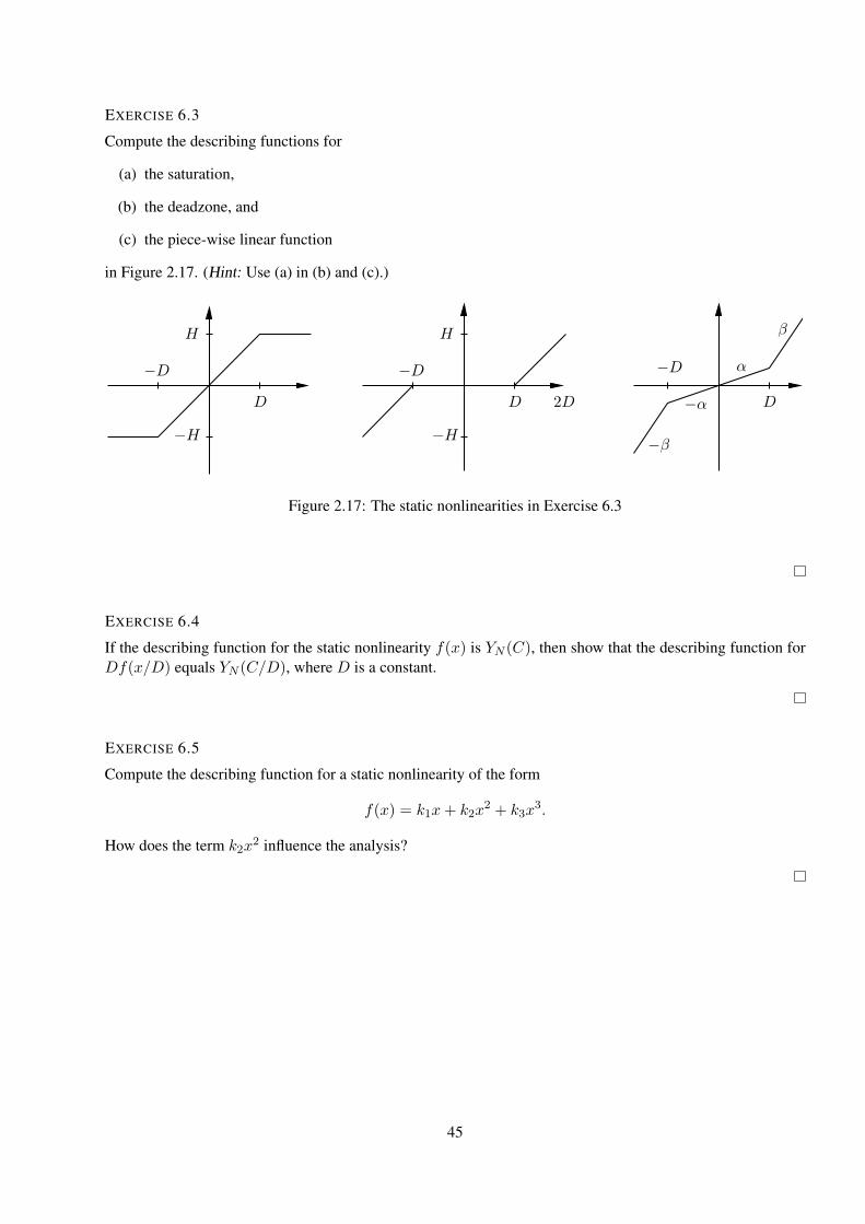
EXERCISE 6.3
Compute the describing functions for
(a) the saturation,
(b) the deadzone, and
(c) the piece-wise linear function
in Figure 2.17. (Hint: Use (a) in (b) and (c).)
DDD
−D−D−D
HH
−H−H
2D
α
β
−α
−β
Figure 2.17: The static nonlinearities in Exercise 6.3
EXERCISE 6.4
If the describing function for the static nonlinearity f(x) is YN (C), then show that the describing function forDf(x/D) equals YN (C/D), where D is a constant.
EXERCISE 6.5
Compute the describing function for a static nonlinearity of the form
f(x) = k1x+ k2x2 + k3x
3.
How does the term k2x2 influence the analysis?
45
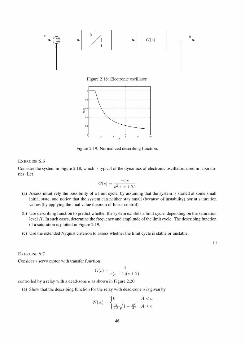
1
k yrΣ G(s)
Figure 2.18: Electronic oscillator.
0 2 4 6 8 100
0.2
0.4
0.6
0.8
1
A
N(A
)
Figure 2.19: Normalized describing function.
EXERCISE 6.6
Consider the system in Figure 2.18, which is typical of the dynamics of electronic oscillators used in laborato-ries. Let
G(s) =−5s
s2 + s+ 25
(a) Assess intuitively the possibility of a limit cycle, by assuming that the system is started at some smallinitial state, and notice that the system can neither stay small (because of instability) nor at saturationvalues (by applying the final value theorem of linear control).
(b) Use describing function to predict whether the system exhibits a limit cycle, depending on the saturationlevelH . In such cases, determine the frequency and amplitude of the limit cycle. The describing functionof a saturation is plotted in Figure 2.19.
(c) Use the extended Nyquist criterion to assess whether the limit cycle is stable or unstable.
EXERCISE 6.7
Consider a servo motor with transfer function
G(s) =4
s(s+ 1)(s+ 2)
controlled by a relay with a dead-zone a as shown in Figure 2.20.
(a) Show that the describing function for the relay with dead-zone a is given by
N(A) =
0 A < a
4πA
√1− a2
A2 A ≥ a
46
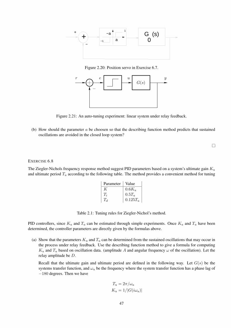
+−
+ G (s) 0a
−a1
−1
Figure 2.20: Position servo in Exercise 6.7.
r e u y
−G(s)
Figure 2.21: An auto-tuning experiment: linear system under relay feedback.
(b) How should the parameter a be choosen so that the describing function method predicts that sustainedoscillations are avoided in the closed loop system?
EXERCISE 6.8
The Ziegler-Nichols frequency response method suggest PID parameters based on a system’s ultimate gain Ku
and ultimate period Tu according to the following table. The method provides a convenient method for tuning
Parameter ValueK 0.6Ku
Ti 0.5TuTd 0.125Tu
Table 2.1: Tuning rules for Ziegler-Nichol’s method.
PID controllers, since Ku and Tu can be estimated through simple experiments. Once Ku and Tu have beendetermined, the controller parameters are directly given by the formulas above.
(a) Show that the parameters Ku and Tu can be determined from the sustained oscillations that may occur inthe process under relay feedback. Use the describing function method to give a formula for computingKu and Tu based on oscillation data. (amplitude A and angular frequency ω of the oscillation). Let therelay amplitude be D.
Recall that the ultimate gain and ultimate period are defined in the following way. Let G(s) be thesystems transfer function, and ωu be the frequency where the system transfer function has a phase lag of−180 degrees. Then we have
Tu = 2π/ωu
Ku = 1/|G(iωu)|
47
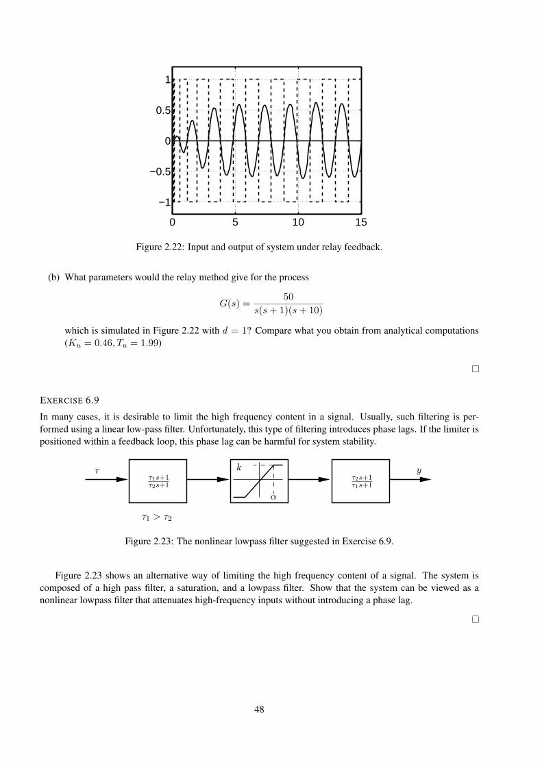
0 5 10 15
−1
−0.5
0
0.5
1
Figure 2.22: Input and output of system under relay feedback.
(b) What parameters would the relay method give for the process
G(s) =50
s(s+ 1)(s+ 10)
which is simulated in Figure 2.22 with d = 1? Compare what you obtain from analytical computations(Ku = 0.46, Tu = 1.99)
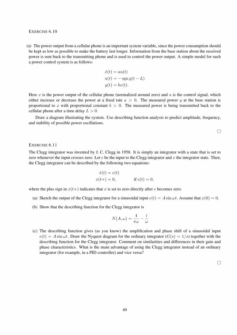
EXERCISE 6.9
In many cases, it is desirable to limit the high frequency content in a signal. Usually, such filtering is per-formed using a linear low-pass filter. Unfortunately, this type of filtering introduces phase lags. If the limiter ispositioned within a feedback loop, this phase lag can be harmful for system stability.
r yτ1s+1τ2s+1
τ2s+1τ1s+1
α
k
τ1 > τ2
Figure 2.23: The nonlinear lowpass filter suggested in Exercise 6.9.
Figure 2.23 shows an alternative way of limiting the high frequency content of a signal. The system iscomposed of a high pass filter, a saturation, and a lowpass filter. Show that the system can be viewed as anonlinear lowpass filter that attenuates high-frequency inputs without introducing a phase lag.
48
EXERCISE 6.10
(a) The power output from a cellular phone is an important system variable, since the power consumption shouldbe kept as low as possible to make the battery last longer. Information from the base station about the receivedpower is sent back to the transmitting phone and is used to control the power output. A simple model for sucha power control system is as follows:
x(t) = au(t)
u(t) = − sgn y(t− L)
y(t) = bx(t).
Here x is the power output of the cellular phone (normalized around zero) and u is the control signal, whicheither increase or decrease the power at a fixed rate a > 0. The measured power y at the base station isproportional to x with proportional constant b > 0. The measured power is being transmitted back to thecellular phone after a time delay L > 0.
Draw a diagram illustrating the system. Use describing function analysis to predict amplitude, frequency,and stability of possible power oscillations.
EXERCISE 6.11
The Clegg integrator was invented by J. C. Clegg in 1958. It is simply an integrator with a state that is set tozero whenever the input crosses zero. Let e be the input to the Clegg integrator and x the integrator state. Then,the Clegg integrator can be described by the following two equations:
x(t) = e(t)
x(t+) = 0, if e(t) = 0,
where the plus sign in x(t+) indicates that x is set to zero directly after e becomes zero.
(a) Sketch the output of the Clegg integrator for a sinusoidal input e(t) = A sinωt. Assume that x(0) = 0.
(b) Show that the describing function for the Clegg integrator is
N(A,ω) =4
πω− i
ω
(c) The describing function gives (as you know) the amplification and phase shift of a sinusoidal inpute(t) = A sinωt. Draw the Nyquist diagram for the ordinary integrator (G(s) = 1/s) together with thedescribing function for the Clegg integrator. Comment on similarities and differences in their gain andphase characteristics. What is the main advantage of using the Clegg integrator instead of an ordinaryintegrator (for example, in a PID controller) and vice versa?
49
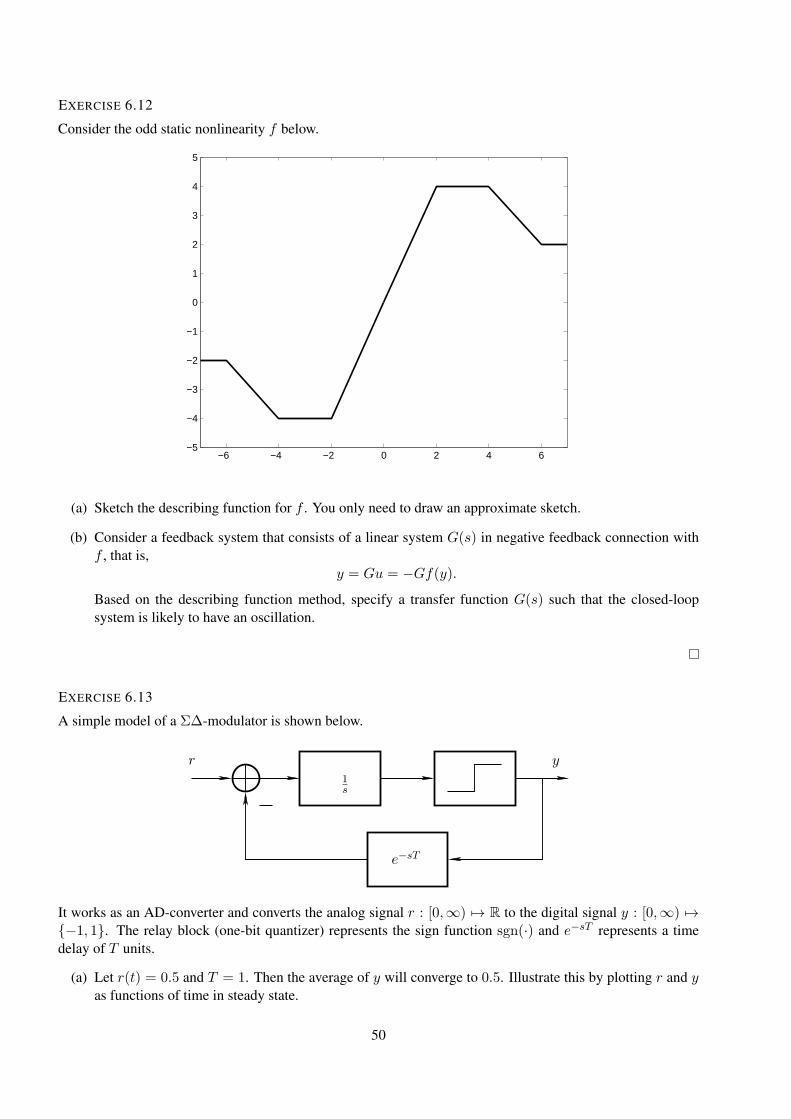
EXERCISE 6.12
Consider the odd static nonlinearity f below.
−6 −4 −2 0 2 4 6−5
−4
−3
−2
−1
0
1
2
3
4
5
(a) Sketch the describing function for f . You only need to draw an approximate sketch.
(b) Consider a feedback system that consists of a linear system G(s) in negative feedback connection withf , that is,
y = Gu = −Gf(y).Based on the describing function method, specify a transfer function G(s) such that the closed-loopsystem is likely to have an oscillation.
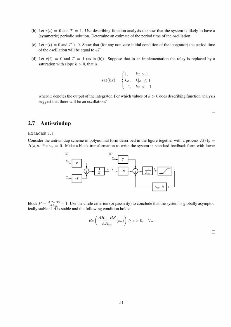
EXERCISE 6.13
A simple model of a Σ∆-modulator is shown below.
r y1s
e−sT
It works as an AD-converter and converts the analog signal r : [0,∞) 7→ R to the digital signal y : [0,∞) 7→−1, 1. The relay block (one-bit quantizer) represents the sign function sgn(·) and e−sT represents a timedelay of T units.
(a) Let r(t) = 0.5 and T = 1. Then the average of y will converge to 0.5. Illustrate this by plotting r and yas functions of time in steady state.
50
(b) Let r(t) = 0 and T = 1. Use describing function analysis to show that the system is likely to have a(symmetric) periodic solution. Determine an estimate of the period time of the oscillation.
(c) Let r(t) = 0 and T > 0. Show that (for any non-zero initial condition of the integrator) the period timeof the oscillation will be equal to 4T .
(d) Let r(t) = 0 and T = 1 (as in (b)). Suppose that in an implementation the relay is replaced by asaturation with slope k > 0, that is,
sat(kx) =
1, kx > 1
kx, k|x| ≤ 1
−1, kx < −1
where x denotes the output of the integrator. For which values of k > 0 does describing function analysissuggest that there will be an oscillation?
2.7 Anti-windup
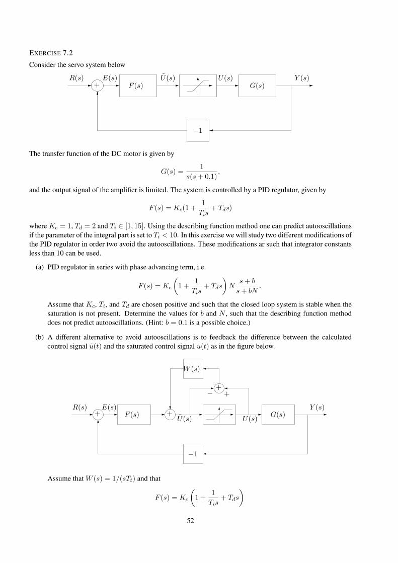
EXERCISE 7.1
Consider the antiwindup scheme in polynomial form described in the figure together with a process A(s)y =B(s)u. Put uc = 0. Make a block transformation to write the system in standard feedback form with lower
u1
R
y−S
uc
∑
T
uc
v u1
Aaw
Aaw− R
y−S ∑
T
(a) (b)
block P = AR+BSAAaw
− 1. Use the circle criterion (or passivity) to conclude that the system is globally asymptot-ically stable if A is stable and the following condition holds:
Re
(AR+BS
AAaw(iω)
)≥ ǫ > 0, ∀ω.
51
EXERCISE 7.2
Consider the servo system below
R(s) E(s) U(s) U(s) Y (s)+
−1
G(s)F (s)
The transfer function of the DC motor is given by
G(s) =1
s(s+ 0.1),
and the output signal of the amplifier is limited. The system is controlled by a PID regulator, given by
F (s) = Kc(1 +1
Tis+ Tds)
where Kc = 1, Td = 2 and Ti ∈ [1, 15]. Using the describing function method one can predict autooscillationsif the parameter of the integral part is set to Ti < 10. In this exercise we will study two different modifications ofthe PID regulator in order two avoid the autooscillations. These modifications ar such that integrator constantsless than 10 can be used.
(a) PID regulator in series with phase advancing term, i.e.
F (s) = Kc
(1 +
1
Tis+ Tds
)N
s+ b
s+ bN.
Assume that Kc, Ti, and Td are chosen positive and such that the closed loop system is stable when thesaturation is not present. Determine the values for b and N , such that the describing function methoddoes not predict autooscillations. (Hint: b = 0.1 is a possible choice.)
(b) A different alternative to avoid autooscillations is to feedback the difference between the calculatedcontrol signal u(t) and the saturated control signal u(t) as in the figure below.
R(s) E(s)
U(s) U(s)
Y (s)
++
++
−
−1
G(s)F (s)
W (s)
Assume that W (s) = 1/(sTt) and that
F (s) = Kc
(1 +
1
Tis+ Tds
)
52
where Kc = 0.95, Ti = 3.8, and Td = 1.68. If the saturation is neglected, the closed loop systems polesare given by the zeros of the characteristic polynomial
(s+ αω0)(s2 + 2ζω0s+ ω2
0)
where ω0 = 0.5, ζ = 0.7, and α = 2. Determine the value of Tt for which the describing functionmethod does not predict autooscillations.
(c) What are advantages and drawbacks of the methods in (a) and (b).
EXERCISE 7.3
Rewrite the blockdiagram of a PI controller with antiwindup (Lecture 7 slide 5) on state-space form as in slide10.
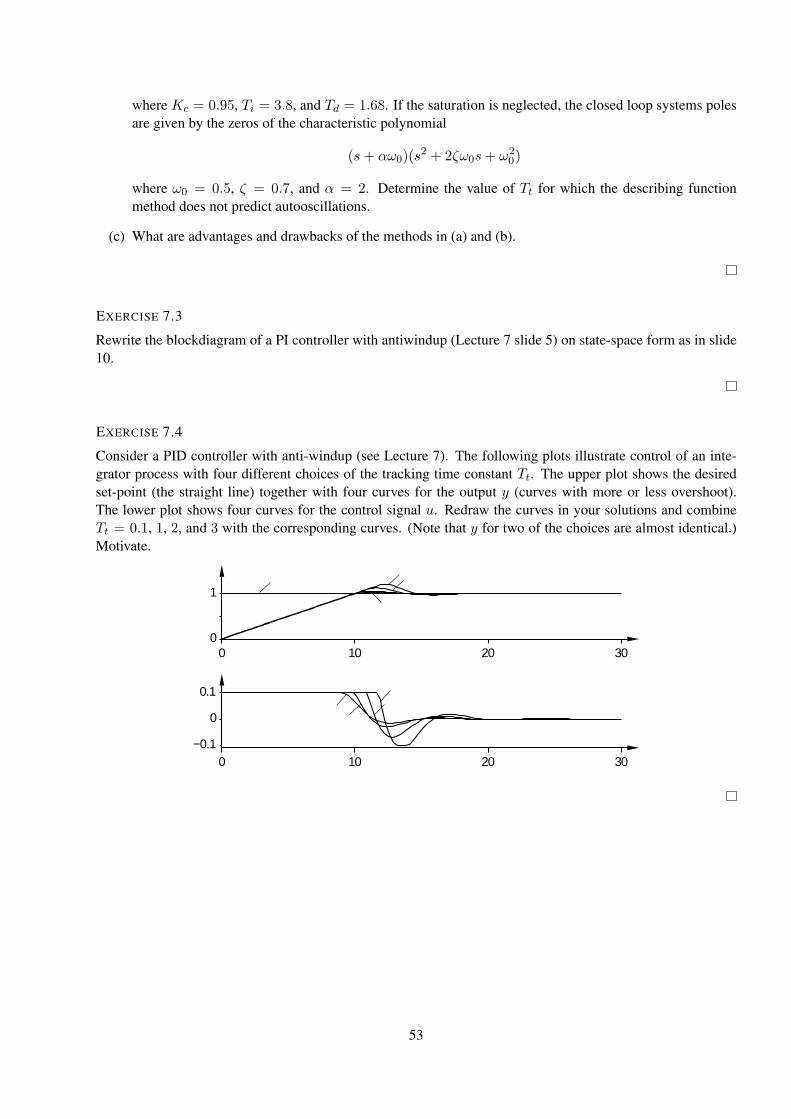
EXERCISE 7.4
Consider a PID controller with anti-windup (see Lecture 7). The following plots illustrate control of an inte-grator process with four different choices of the tracking time constant Tt. The upper plot shows the desiredset-point (the straight line) together with four curves for the output y (curves with more or less overshoot).The lower plot shows four curves for the control signal u. Redraw the curves in your solutions and combineTt = 0.1, 1, 2, and 3 with the corresponding curves. (Note that y for two of the choices are almost identical.)Motivate.
0 10 20 300
1
0 10 20 30−0.1
0
0.1
53
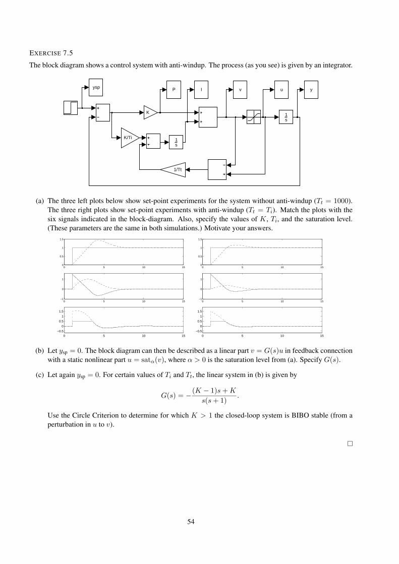
EXERCISE 7.5
The block diagram shows a control system with anti-windup. The process (as you see) is given by an integrator.
ysp yIP uv
K/Ti
K 1s
1s
1/Tt
(a) The three left plots below show set-point experiments for the system without anti-windup (Tt = 1000).The three right plots show set-point experiments with anti-windup (Tt = Ti). Match the plots with thesix signals indicated in the block-diagram. Also, specify the values of K, Ti, and the saturation level.(These parameters are the same in both simulations.) Motivate your answers.
0 5 10 150
0.5
1
1.5
0 5 10 15−1
0
1
0 5 10 15−0.5
0
0.5
1
1.5
0 5 10 150
0.5
1
1.5
0 5 10 15−1
0
1
0 5 10 15−0.5
0
0.5
1
1.5
(b) Let ysp = 0. The block diagram can then be described as a linear part v = G(s)u in feedback connectionwith a static nonlinear part u = satα(v), where α > 0 is the saturation level from (a). Specify G(s).
(c) Let again ysp = 0. For certain values of Ti and Tt, the linear system in (b) is given by
G(s) = −(K − 1)s+K
s(s+ 1).
Use the Circle Criterion to determine for which K > 1 the closed-loop system is BIBO stable (from aperturbation in u to v).
54
2.8 Friction, Backlash and Quantization
EXERCISE 8.1
The following model for friction is described in a recent PhD thesis
dz
dt= v − |v|
g(v)z
F = σ0z + σ1(v)dz
dt+ Fvv,
where σ0, Fv are positive constants and g(v) and σ1(v) are positive functions of velocity.
(a) What friction force does the model give for constant velocity?
(b) Prove that the map from v to z is passive if z(0) = 0.
(c) Prove that the map from v to F is passive if z(0) = 0 if 0 ≤ σ1(v) ≤ 4σ0g(v)/|v|.
EXERCISE 8.2
Derive the describing function (v input, F output) for
(a) Coulomb friction, F = F0sign (v)
(b) Coulomb + linear viscous friction F = F0sign (v) + Fvv
(c) as in b) but with stiction for v = 0.
EXERCISE 8.3
If v is not directly measurable the adaptive friction compensation scheme in the lectures must be changed.Consider the following double observer scheme:
F = (zF +KF |v|)sign(v)
zF = −KF (u− F )sign(v)
v = zv +Kvx
zv = −F + u−Kv v.
Show that linearisation of the error equations
˙ev = v − ˙v = gv(ev, eF , v, F )
˙eF = F − ˙F = gF (ev, eF , v, F )
gives Jacobian
A =
[−Kv −1
−KvKF 0
].
Conclude that local error convergence is achieved if Kv > 0 and KF < 0.
EXERCISE 8.4
55
Show that the describing function for quantization is given by
N(A) =
0 A < D2
4D
πA
n∑i=1
√1−
(2i− 1
2AD
)22n−1
2 D < A < 2n+12 D
(Hint: Use one of the nonlinearities from lecture 8 and superposition.)
EXERCISE 8.5
Show that a saturation is a passive element.
EXERCISE 8.6
Consider the mass-spring system with dry friction
y + cy + ky + η(y, y) = 0
where η is defined as
η(y, y) =
µkmgsign(y) for |y| > 0
−ky for y = 0 and |y| ≤ µsmg/k
−µsmgsign(y) for y = 0 and |y| > µsmg/k
Construct the phase potrait and discuss its qualitative behavior. (Hint: Use piecewise linear analysis.)
EXERCISE 8.7
The accuracy of a crude A/D converter can be improved by adding a high-frequency dither signal before quan-tization and lowpass filtering the discretized signal, see Figure 2.24 Compute the stationary value y0 of the
A/D filter decim.+
Figure 2.24: A/D converter in Exercise 8.7
output if the input is a constant u0. The dither signal is a triangle wave with zero mean and amplitude D/2where D is the quantization level.
56
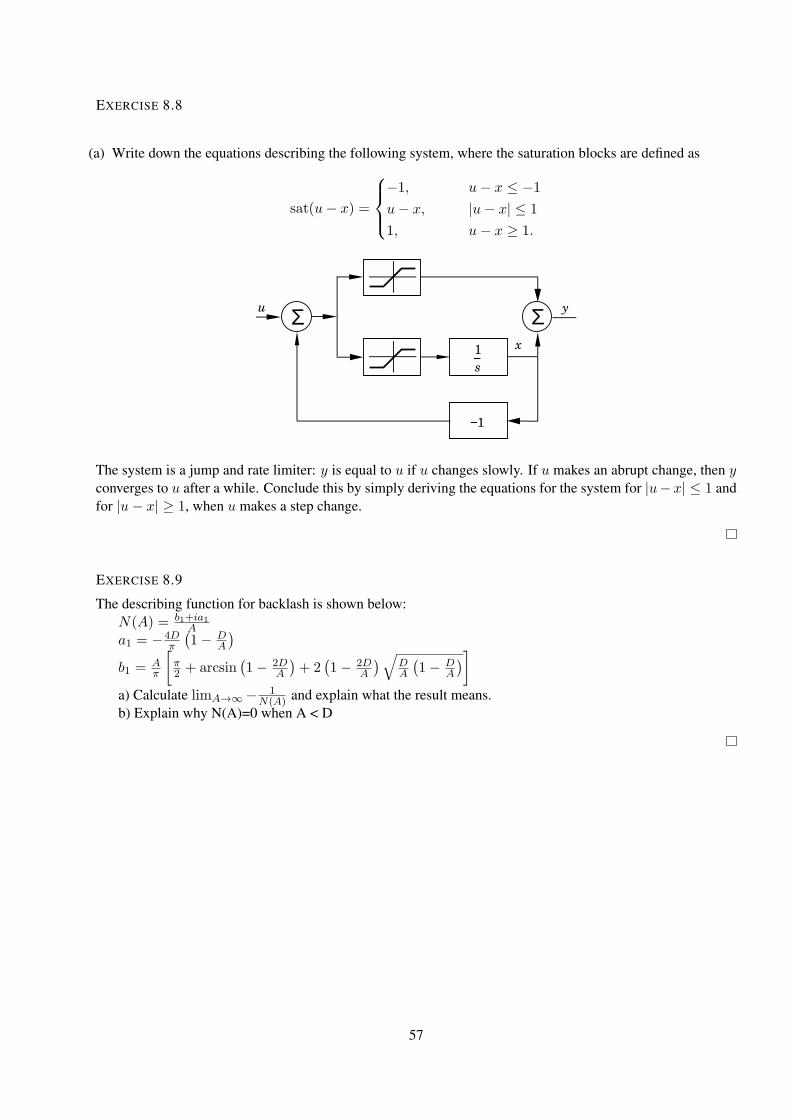
EXERCISE 8.8
(a) Write down the equations describing the following system, where the saturation blocks are defined as
sat(u− x) =
−1, u− x ≤ −1
u− x, |u− x| ≤ 1
1, u− x ≥ 1.
yΣu Σ
1
s
−1
x
The system is a jump and rate limiter: y is equal to u if u changes slowly. If u makes an abrupt change, then yconverges to u after a while. Conclude this by simply deriving the equations for the system for |u−x| ≤ 1 andfor |u− x| ≥ 1, when u makes a step change.
EXERCISE 8.9
The describing function for backlash is shown below:N(A) = b1+ia1
Aa1 = −4D
π
(1− D
A
)
b1 =Aπ
[π2 + arcsin
(1− 2D
A
)+ 2
(1− 2D
A
)√DA
(1− D
A
)]
a) Calculate limA→∞− 1N(A) and explain what the result means.
b) Explain why N(A)=0 when A < D
57
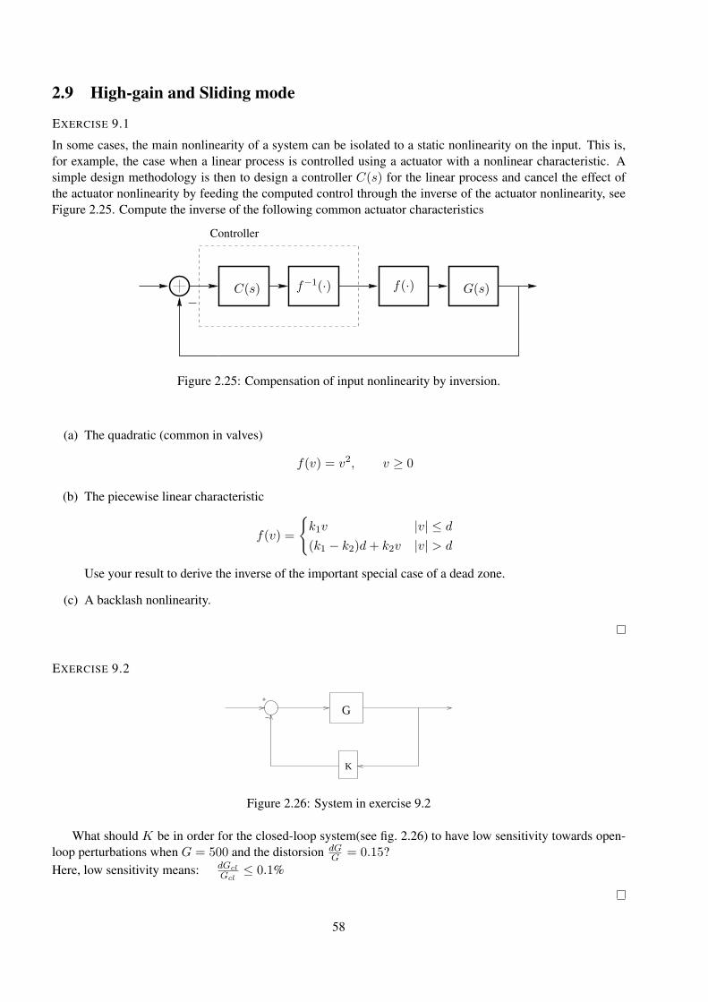
2.9 High-gain and Sliding mode
EXERCISE 9.1
In some cases, the main nonlinearity of a system can be isolated to a static nonlinearity on the input. This is,for example, the case when a linear process is controlled using a actuator with a nonlinear characteristic. Asimple design methodology is then to design a controller C(s) for the linear process and cancel the effect ofthe actuator nonlinearity by feeding the computed control through the inverse of the actuator nonlinearity, seeFigure 2.25. Compute the inverse of the following common actuator characteristics
C(s) f−1(·) f(·) G(s)−
Controller
Figure 2.25: Compensation of input nonlinearity by inversion.
(a) The quadratic (common in valves)
f(v) = v2, v ≥ 0
(b) The piecewise linear characteristic
f(v) =
k1v |v| ≤ d
(k1 − k2)d+ k2v |v| > d
Use your result to derive the inverse of the important special case of a dead zone.
(c) A backlash nonlinearity.
EXERCISE 9.2
+
−
K
G
Figure 2.26: System in exercise 9.2
What should K be in order for the closed-loop system(see fig. 2.26) to have low sensitivity towards open-loop perturbations when G = 500 and the distorsion dG
G = 0.15?Here, low sensitivity means: dGcl
Gcl≤ 0.1%
58
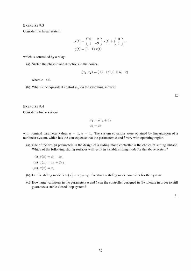
EXERCISE 9.3
Consider the linear system
x(t) =
(0 −21 −3
)x(t) +
(01
)u
y(t) =(0 1
)x(t)
which is controlled by a relay.
(a) Sketch the phase-plane directions in the points.
(x1, x2) = (±2,±ε), (±0.5,±ε)
where ε→ 0.
(b) What is the equivalent control ueq on the switching surface?
EXERCISE 9.4
Consider a linear system
x1 = ax2 + bu
x2 = x1
with nominal parameter values a = 1, b = 1. The system equations were obtained by linearization of anonlinear system, which has the consequence that the parameters a and b vary with operating region.
(a) One of the design parameters in the design of a sliding mode controller is the choice of sliding surface.Which of the following sliding surfaces will result in a stable sliding mode for the above system?
(i) σ(x) = x1 − x2
(ii) σ(x) = x1 + 2x2
(iii) σ(x) = x1
(b) Let the sliding mode be σ(x) = x1 + x2. Construct a sliding mode controller for the system.
(c) How large variations in the parameters a and b can the controller designed in (b) tolerate in order to stillguarantee a stable closed loop system?
59
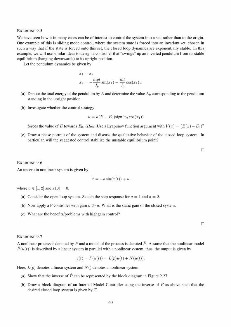
EXERCISE 9.5
We have seen how it in many cases can be of interest to control the system into a set, rather than to the origin.One example of this is sliding mode control, where the system state is forced into an invariant set, chosen insuch a way that if the state is forced onto this set, the closed loop dynamics are exponentially stable. In thisexample, we will use similar ideas to design a controller that “swings” up an inverted pendulum from its stableequilibrium (hanging downwards) to its upright position.
Let the pendulum dynamics be given by
x1 = x2
x2 = −mglJp
sin(x1)−ml
Jpcos(x1)u
(a) Denote the total energy of the pendulum byE and determine the valueE0 corresponding to the pendulumstanding in the upright position.
(b) Investigate whether the control strategy
u = k(E − E0)sign(x2 cos(x1))
forces the value of E towards E0. (Hint. Use a Lyapunov function argument with V (x) = (E(x)−E0)2
(c) Draw a phase portrait of the system and discuss the qualitative behavior of the closed loop system. Inparticular, will the suggested control stabilize the unstable equilibrium point?
EXERCISE 9.6
An uncertain nonlinear system is given by
x = −a sin(x(t)) + u
where a ∈ [1, 2] and x(0) = 0.
(a) Consider the open loop system. Sketch the step response for a = 1 and a = 2.
(b) Now apply a P controller with gain k ≫ a. What is the static gain of the closed system.
(c) What are the benefits/problems with highgain control?
EXERCISE 9.7
A nonlinear process is denoted by P and a model of the process is denoted P . Assume that the nonlinear modelP (u(t)) is described by a linear system in parallel with a nonlinear system, thus, the output is given by
y(t) = P (u(t)) = L(p)u(t) +N(u(t)).
Here, L(p) denotes a linear system and N() denotes a nonlinear system.
(a) Show that the inverse of P can be represented by the block diagram in Figure 2.27.
(b) Draw a block diagram of an Internal Model Controller using the inverse of P as above such that thedesired closed loop system is given by T .
60
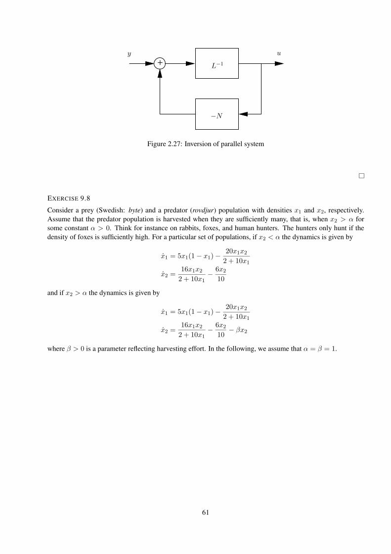
+ L−1
−N
uy
Figure 2.27: Inversion of parallel system
EXERCISE 9.8
Consider a prey (Swedish: byte) and a predator (rovdjur) population with densities x1 and x2, respectively.Assume that the predator population is harvested when they are sufficiently many, that is, when x2 > α forsome constant α > 0. Think for instance on rabbits, foxes, and human hunters. The hunters only hunt if thedensity of foxes is sufficiently high. For a particular set of populations, if x2 < α the dynamics is given by
x1 = 5x1(1− x1)−20x1x22 + 10x1
x2 =16x1x22 + 10x1
− 6x210
and if x2 > α the dynamics is given by
x1 = 5x1(1− x1)−20x1x22 + 10x1
x2 =16x1x22 + 10x1
− 6x210
− βx2
where β > 0 is a parameter reflecting harvesting effort. In the following, we assume that α = β = 1.
61
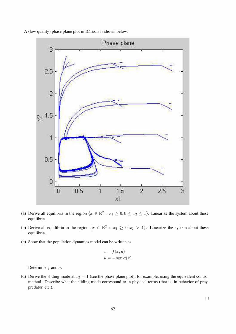
A (low quality) phase plane plot in ICTools is shown below.
(a) Derive all equilibria in the region x ∈ R2 : x1 ≥ 0, 0 ≤ x2 ≤ 1. Linearize the system about these
equilibria.
(b) Derive all equilibria in the region x ∈ R2 : x1 ≥ 0, x2 > 1. Linearize the system about these
equilibria.
(c) Show that the population dynamics model can be written as
x = f(x, u)
u = − sgnσ(x).
Determine f and σ.
(d) Derive the sliding mode at x2 = 1 (see the phase plane plot), for example, using the equivalent controlmethod. Describe what the sliding mode correspond to in physical terms (that is, in behavior of prey,predator, etc.).
62
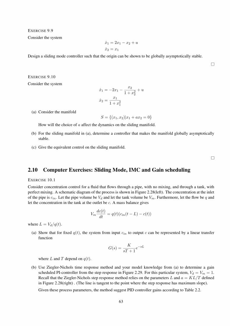
EXERCISE 9.9
Consider the systemx1 = 2x1 − x2 + u
x2 = x1
Design a sliding mode controller such that the origin can be shown to be globally asymptotically stable.
EXERCISE 9.10
Consider the systemx1 = −2x1 −
x21 + x22
+ u
x2 =x1
1 + x21
(a) Consider the manifoldS = (x1, x2)|x1 + ax2 = 0
How will the choice of a affect the dynamics on the sliding manifold.
(b) For the sliding manifold in (a), determine a controller that makes the manifold globally asymptoticallystable.
(c) Give the equivalent control on the sliding manifold.
2.10 Computer Exercises: Sliding Mode, IMC and Gain scheduling
EXERCISE 10.1
Consider concentration control for a fluid that flows through a pipe, with no mixing, and through a tank, withperfect mixing. A schematic diagram of the process is shown in Figure 2.28(left). The concentration at the inletof the pipe is cin. Let the pipe volume be Vd and let the tank volume be Vm. Furthermore, let the flow be q andlet the concentration in the tank at the outlet be c. A mass balance gives
Vmdc(t)
dt= q(t)(cin(t− L)− c(t))
where L = Vd/q(t).
(a) Show that for fixed q(t), the system from input cin to output c can be represented by a linear transferfunction
G(s) =K
sT + 1e−sL
where L and T depend on q(t).
(b) Use Ziegler-Nichols time response method and your model knowledge from (a) to determine a gainscheduled PI-controller from the step response in Figure 2.29. For this particular system, Vd = Vm = 1.Recall that the Ziegler-Nichols step response method relies on the parameters L and a = KL/T definedin Figure 2.28(right) . (The line is tangent to the point where the step response has maximum slope).
Given these process parameters, the method suggest PID controller gains according to Table 2.2.
63
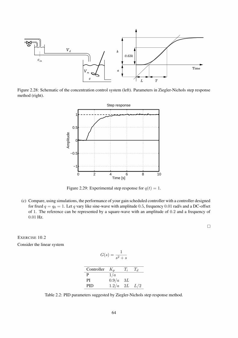
cin
Vd
Vm
c
k
a
L T
Time
0.63k
Figure 2.28: Schematic of the concentration control system (left). Parameters in Ziegler-Nichols step responsemethod (right).
0 2 4 6 8 10
−1
−0.5
0
0.5
1
Time [s]
Am
plitu
de
Step response
Figure 2.29: Experimental step response for q(t) = 1.
(c) Compare, using simulations, the performance of your gain scheduled controller with a controller designedfor fixed q = q0 = 1. Let q vary like sine-wave with amplitude 0.5, frequency 0.01 rad/s and a DC-offsetof 1. The reference can be represented by a square-wave with an amplitude of 0.2 and a frequency of0.01 Hz.
EXERCISE 10.2
Consider the linear system
G(s) =1
s2 + s
Controller Kp Ti TdP 1/aPI 0.9/a 3LPID 1.2/a 2L L/2
Table 2.2: PID parameters suggested by Ziegler-Nichols step response method.
64
and simulate an on-off control. Hence, let the controller be relay with output ±1. Plot the step response for astep starting at t = 0 (Simulation is troublesome if r = 0). What happens if there is a measurement disturbance(a step with amplitude 0.1) appears at t = 20? What about the control signal?
EXERCISE 10.3
Consider the linear system in Exercise 9.4 where the system is given by
x1 = ax2 + bu
x2 = x1
with nominal parameter values a = 1, b = 1. Using the sliding surface σ(x) = x1 + x2 and a = b = 1 we getthe sliding controller
u = −(x1 + x2)− µsign(x1 + x2).
Implement the controller and try different values of a, b and µ. Plot x1 on one axis and x2 on the other. Trydifferent initial conditions, far away and close to the line x2 = −x1 which is the sliding surface.
Please note that when simulating systems controlled by a sliding mode controller Matlab/Simulink mayhave difficulties simulating the system when x1 and x2 approaches zero. In these cases, stop the simulation andplot what you get instead of waiting too long for the result.
EXERCISE 10.4
Consider the pendulum given by
x1(t) = x2(t)
x2(t) = −a sin(x1(t) + δ)− bx2(t) + cu(t)
where x1 = θ − δ and x2 = θ. A sliding surface σ(x) = x1 + x2, gives the sliding mode controller
u = −1
c(x2 − a sin(x1 + δ)− bx2)−
µ
csign(x1 + x2).
Simulate the controller using a = 1.5, b = 0.75, c = 0.75 and δ = π4 . For the controller use a = b = c = µ =
1. Try different values of µ.
65
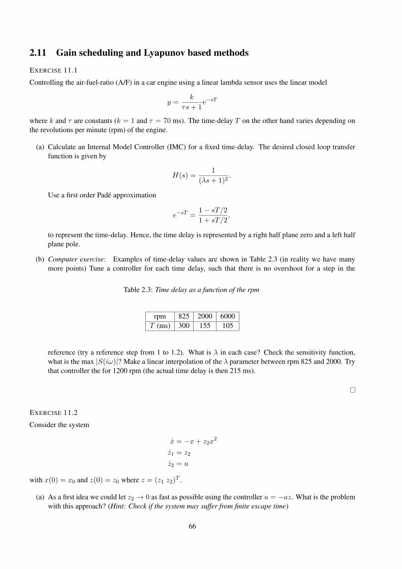
2.11 Gain scheduling and Lyapunov based methods
EXERCISE 11.1
Controlling the air-fuel-ratio (A/F) in a car engine using a linear lambda sensor uses the linear model
y =k
τs+ 1e−sT
where k and τ are constants (k = 1 and τ = 70 ms). The time-delay T on the other hand varies depending onthe revolutions per minute (rpm) of the engine.
(a) Calculate an Internal Model Controller (IMC) for a fixed time-delay. The desired closed loop transferfunction is given by
H(s) =1
(λs+ 1)2.
Use a first order Padé approximation
e−sT =1− sT/2
1 + sT/2,
to represent the time-delay. Hence, the time delay is represented by a right half plane zero and a left halfplane pole.
(b) Computer exercise: Examples of time-delay values are shown in Table 2.3 (in reality we have manymore points) Tune a controller for each time delay, such that there is no overshoot for a step in the
Table 2.3: Time delay as a function of the rpm
rpm 825 2000 6000T (ms) 300 155 105
reference (try a reference step from 1 to 1.2). What is λ in each case? Check the sensitivity function,what is the max |S(iω)|? Make a linear interpolation of the λ parameter between rpm 825 and 2000. Trythat controller the for 1200 rpm (the actual time delay is then 215 ms).
EXERCISE 11.2
Consider the system
x = −x+ z2x2
z1 = z2
z2 = u
with x(0) = x0 and z(0) = z0 where z = (z1 z2)T .
(a) As a first idea we could let z2 → 0 as fast as possible using the controller u = −az. What is the problemwith this approach? (Hint: Check if the system may suffer from finite escape time)
66
(b) Consider the more general form of the system
x = f0(x) + yT f(x, z)
z = Az +Bu
y = Cz
and use the controller
u = Kz − 1
2
∂V
∂xf(x, z) (2.7)
where V (x) is the Lyapunov function for the system x = f0(x). The matrix K satisfies the positive realcondition
(A+BK)TP + P (A+BK) = −Qand PB = CT
for some P > 0 and Q ≥ 0.
(c) Study the global asymptotic stability using the Lyapunov function
W (x, z) = V (x) + zTPz.
EXERCISE 11.3
Consider the uncertain system
x1 = x2
x2 = x31 + x32 + (1 + a)u
where a is an unknown constant which satisfy and |a| ≤ 12 .
EXERCISE 11.4
Consider the uncertain system
x1 = x2
x2 = (1 + a1)(x31 + x32) + (1 + a2)u
where a1 and a2 are unknown constants which satisfy |a1| ≤ 1 and |a2| ≤ 12 .
67
EXERCISE 11.5
Consider the system
x1 = x2
x2 = u+ δ(x)
where δ is unknown but we know an estimate of ρ such that |δ(x)| ≤ ρ‖x‖2. Let u = ψ(x) = −x1 − x2 be thenominal stabilizing controller and
v =
−ρ‖x‖2 w‖w‖2
if ρ‖x‖2‖w‖2 ≥ ǫ
−ρ2‖x‖22wǫ if ρ‖x‖2‖w‖2 < ǫ
where wT = 2xTPB and V (x) = xTPx is a Lyapunov function for the nominal closed loop system.Show that when δ(x) = 2(x1 + x2) and ρ = 2
√2 the origin is unstable.
EXERCISE 11.6
Consider the system
x1 = x21 − x31 + x2
x2 = u.
Compute a controller using backstepping to globally stabilize the origin.
EXERCISE 11.7
Consider the system
x1 = x21 − x31 + x2
x2 = x3
x3 = u.
Compute a controller using backstepping to globally stabilize the origin.
EXERCISE 11.8
Consider the system
x1 = −x1 + x21x2
x2 = u
compute a controller to obtain global stabilization using the backstepping approach.
68
EXERCISE 11.9
Consider the system
x1 = x1x2
x2 = x1 + u
compute a controller using backstepping to globally stabilize the origin.
EXERCISE 11.10
Consider the system
x1 = x2 + a+ (x1 − a1/3)3
x2 = x1 + u
where a is a constant. Compute a controller using backstepping to globally stabilize the origin.
EXERCISE 11.11
The equations of motion of an m-link robot is described by
M(q)q + C(q, q)q + g(q) = u
where q is an m-dimensional vector of generalized coordinates representing joint positions. The control torqueinput is represented by u and M(q) is a symmetric inertia matrix which is positive definite ∀q ∈ Rm. Theterm C(q, q)q accounts for centrifugal and Coriolis forces. The matrix C has the property that M − sC is askew-symmetric matrix ∀q, q ∈ Rm, where M is the total derivative of M with respect to t. The term g(q),
which accounts for gravity forces, is given by g(q) =[∂P (q)∂q
]Twhere P (q) is the total potential energy of the
links due to gravity. We will assume that P (q) is positive definite function of q and g(q) = 0 has an isolatedroot at q = 0.
(a) With u = 0 use the total energy
V (q, q) =1
2qTM(q)q + P (q)
as a Lyapunov function candidate to show that the origin (q = 0, q = 0) is stable.
(b) With u = −Kdq where Kd is a positive diagonal matrix, show that the origin is asymptotically stable.
(c) With u = g(q)−Kp(q− q∗)−Kdq where Kp and Kd are positive diagonal matrices. and q∗ is a desiredrobot position in Rm, show that the point (q = q∗, q = 0) is an asymptotically stable equilibrium point.
69
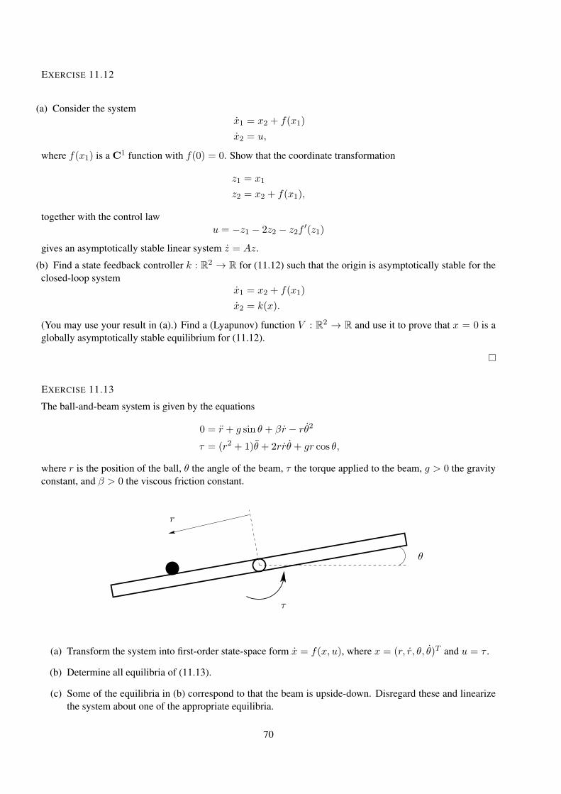
EXERCISE 11.12
(a) Consider the systemx1 = x2 + f(x1)
x2 = u,
where f(x1) is a C1 function with f(0) = 0. Show that the coordinate transformation
z1 = x1
z2 = x2 + f(x1),
together with the control lawu = −z1 − 2z2 − z2f
′(z1)
gives an asymptotically stable linear system z = Az.
(b) Find a state feedback controller k : R2 → R for (11.12) such that the origin is asymptotically stable for theclosed-loop system
x1 = x2 + f(x1)
x2 = k(x).
(You may use your result in (a).) Find a (Lyapunov) function V : R2 → R and use it to prove that x = 0 is aglobally asymptotically stable equilibrium for (11.12).
EXERCISE 11.13
The ball-and-beam system is given by the equations
0 = r + g sin θ + βr − rθ2
τ = (r2 + 1)θ + 2rrθ + gr cos θ,
where r is the position of the ball, θ the angle of the beam, τ the torque applied to the beam, g > 0 the gravityconstant, and β > 0 the viscous friction constant.
r
θ
τ
(a) Transform the system into first-order state-space form x = f(x, u), where x = (r, r, θ, θ)T and u = τ .
(b) Determine all equilibria of (11.13).
(c) Some of the equilibria in (b) correspond to that the beam is upside-down. Disregard these and linearizethe system about one of the appropriate equilibria.
70
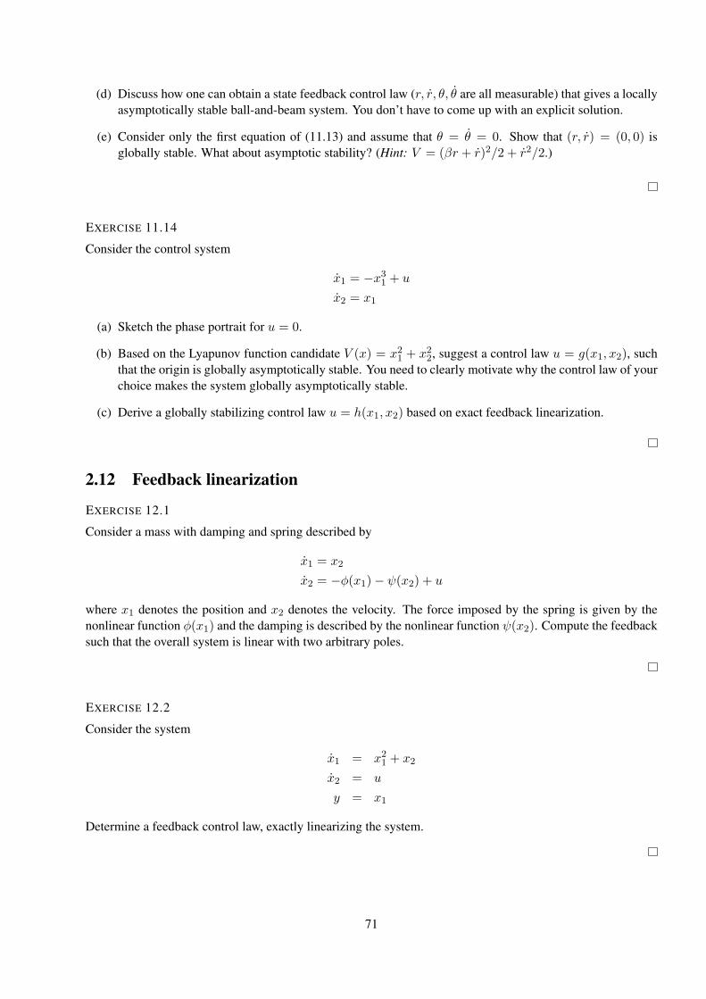
(d) Discuss how one can obtain a state feedback control law (r, r, θ, θ are all measurable) that gives a locallyasymptotically stable ball-and-beam system. You don’t have to come up with an explicit solution.
(e) Consider only the first equation of (11.13) and assume that θ = θ = 0. Show that (r, r) = (0, 0) isglobally stable. What about asymptotic stability? (Hint: V = (βr + r)2/2 + r2/2.)
EXERCISE 11.14
Consider the control system
x1 = −x31 + u
x2 = x1
(a) Sketch the phase portrait for u = 0.
(b) Based on the Lyapunov function candidate V (x) = x21 + x22, suggest a control law u = g(x1, x2), suchthat the origin is globally asymptotically stable. You need to clearly motivate why the control law of yourchoice makes the system globally asymptotically stable.
(c) Derive a globally stabilizing control law u = h(x1, x2) based on exact feedback linearization.
2.12 Feedback linearization
EXERCISE 12.1
Consider a mass with damping and spring described by
x1 = x2
x2 = −φ(x1)− ψ(x2) + u
where x1 denotes the position and x2 denotes the velocity. The force imposed by the spring is given by thenonlinear function φ(x1) and the damping is described by the nonlinear function ψ(x2). Compute the feedbacksuch that the overall system is linear with two arbitrary poles.
EXERCISE 12.2
Consider the system
x1 = x21 + x2
x2 = u
y = x1
Determine a feedback control law, exactly linearizing the system.
71
EXERCISE 12.3
Consider the system with two water tanks
u
x1
x2
The dynamics are given by
x1 = 1 + u−√1 + x1
x2 =√1 + x1 −
√1 + x2
y = x2
(a) Show that the system has a strong relative degree of 2 (r = 2).
(b) Determine the coordinate transformation such that the system can be written as
z1 = z2
z2 = α(z) + β(z)u
y = z1
(c) Determine a feedback control law, exactly linearizing the system.
EXERCISE 12.4
Find a feedback law
u = h(x, v)
that renders the closed loop system from the new input, v to the output, y, linear. Is the zero dynamic stable orunstable?
(a) Consider
x1 = x32
x2 = u
y = x1 + x2
72
(b) Consider
x1 = −x22 + u
x2 = u
y = x1
EXERCISE 12.5
Determine a feedback control lawx1 = −x1 + 7x2
x2 = −x2 + cosx1 + u
exactly linearizing the system.
EXERCISE 12.6
Determine a feedback control law
x1 = x3 + 8x2
x2 = −x2 + x3
x3 = −x3 + x41 − x21 + u
y = x1
exactly linearizing the system.
EXERCISE 12.7
An important class of nonlinear systems can be written on the form
x1 = x2
x2 = x3...
xn = f(x) + g(x)u
Assume that the full state x is available for measurement.
(a) Find a feedback
u = h(x, v)
that renders the closed loop system from the new input v to the state linear. What conditions do you haveto impose on f(x) and g(x) in order to make the procedure well posed?
73
(b) Apply this procedure to design a feedback for the inverted pendulum
x1 = x2
x2 = a sin(x1) + b cos(x2)u
that makes the closed loop system behave as a linear system with a double pole in s = −1. Is the controlwell defined for all x? Can you explain this intuitively?
(c) One drawback with the above procedure is that it is very sensitive to modelling errors. Show that this isthe case by designing a linearizing feedback for the system
x = x2 + u
that makes the closed loop system linear with a pole in −1. Apply the suggested control to the system
x = (1 + ǫ)x2 + u
and show that some solutions are unbounded irrespectively of ǫ 6= 0.
2.13 Optimal Control
EXERCISE 13.1
For a fixed tf > 0, find an optimal control law u∗ that solves
minu
∫ tf
0(x(t) + u2(t)) dt
s.t.x(t) = x(t) + u(t) + 1,
x(0) = 0.
EXERCISE 13.2
Find the optimal control function of the control problem
minu
∫ tf
0dt
s.t.x1(t) = x2(t),
x2(t) = u(t),
x1(0) = x0, x1(tf ) = 0,
x2(0) = v0, x2(tf ) = 0,
‖u(t)‖ ≤ 1 for all t.
74
EXERCISE 13.3
Neglecting air resistance and the curvature of the earth, the launching of a satellite can be described by thefollowing equations
x1 = x3
x2 = x4
x3 =F
mcosu
x4 =F
msinu− g
where (x1, x2) is the coordinate and (x3, x4) the corresponding velocity. The signal u is the controlled angle.Suppose that φ(x(tf )) is the criterion to be minimized and that ψ(x(tf )) = 0 is the end constraint. Show thatthe optimal control signal has the form
tanu∗(t) =At+B
Ct+D
where A,B,C,D are constants (which you do not have to determine).
EXERCISE 13.4
Suppose more realistically that m and F vary. Let u1 be the control signal in previous exercise and u2(t) =F (t). Suppose u2 has limitations
0 ≤ u2(t) ≤ umax
Let the mass m = x3(t) vary asx3 = −γu2
Show that
tanu1 =λ1λ4
and u2 =
umax σ < 00 σ > 0⋆ σ = 0,
where ⋆ means that the solution is unknown. Determine equations for λ and σ. (You do not have to solve theequations).
EXERCISE 13.5
Consider the system x1 = x2x2 = −x1 − x32 + (1 + x1)u
with initial conditions x1(0) = 1, x2(0) = 1 and let the criterion be
minu:[0,1]→R
∫ 1
0(ex
2
1 + x22 + u2) dt.
Show that the extremals satisfy
x1 = f1(x1, x2, λ1, λ2)
x2 = f2(x1, x2, λ1, λ2)
λ1 = f3(x1, x2, λ1, λ2)
λ2 = f4(x1, x2, λ1, λ2)
Determine f1, f2, f3, f4. What conditions must λ1, λ2 satisfy at the end point?
75

EXERCISE 13.6
Consider the double integrator
x1 = x2
x2 = u, |u| ≤ 1
with initial value x(0) = x0. We are interested in finding the control that brings the system to rest (x(tf ) = 0)in minimum time. (You may think of this as a way of designing a controller that reacts quickly to set-pointchanges.)
(a) Show that the optimal control is of “bang-bang type” with at most one switch. (In other words, showthat the optimal control is first maximal in one direction for some time, and then possibly changes signto become maximal in the other direction for the remaining time)
(b) Show that the control can be expressed as a feedback law
u =
umax σ(x) > 0
−umax σ(x) < 0
Derive an explicit formula for the switch function σ(x).
(c) Using a phase plane tool, construct the phase portrait of the closed-loop system under the optimal control.
EXERCISE 13.7
Consider the problem of controlling the double integratorx1 = x2x2 = u, |u| ≤ 1
from an arbitrary initial condition x(0) to the origin so that the criterion
∫ tf
0(1 + |u|) dt
is minimized (tf is the first time so that x(t) = 0). Show that all extremals are of the form
u(t) =
−1 0 ≤ t ≤ t10 t1 ≤ t ≤ t21 t2 ≤ t ≤ tf
or
u(t) =
1 0 ≤ t ≤ t10 t1 ≤ t ≤ t2−1 t2 ≤ t ≤ tf
for some t1, t2 with 0 ≤ t1 ≤ t2 ≤ tf . (Some time interval can thus have length zero.) Assume that theproblem is normal.
76
EXERCISE 13.8
Consider the problem of taking the state of the system
x =
(−5 2−6 2
)x+
(01
)u
from x0 = (0, 0)T to x(tf ) = (1, 1)T in minimum time with |u(t)| ≤ 3. Show that the optimal controller iseither
u(t) =
−3 0 ≤ t ≤ t1+3 t1 ≤ t ≤ tf
or
u(t) =
+3 0 ≤ t ≤ t1−3 t1 ≤ t ≤ tf
for some t1.
EXERCISE 13.9
Show that the minimum-time control of a linear system
x = Ax+Bu, y = Cx, |u| ≤ 1, x(tf ) = 0,
leads to extremals withu(t) = sign σ(t)
Determine σ(t).
EXERCISE 13.10
What is the conclusion from the maximum principle for the problem
min∫ 1
0u dt,
x = u
x(0) = 0
x(1) = 1
EXERCISE 13.11
Consider an optimal heating problem where T is the temperature and P heat effect. Let
T = P − T
0 ≤ P ≤ Pmax
T (0) = 0, T (1) = 1
and solve min∫ 10 P (t) dt.
77
EXERCISE 13.12
In this problem we study the linear quadratic optimal control problem
minu:[0,tf ]→Rm
1
2
∫ tf
0
[x(t)TQx(t) + u(t)TRu(t)
]dt
with
x(t) = Ax(t) +Bu(t), x(0) = x0.
Suppose that tf > 0 and x0 are fixed and that the matrices Q = QT and R = RT are positive definite. Then,the optimal control is given by
u∗(t) = −R−1BTS(t)x(t),
where the matrix S(t) = ST (t) satisfies the differential equation
−S(t) = ATS(t) + S(t)A− S(t)BR−1BTS(t) +Q,
where S(tf ) = 0n×n is an n× n zero matrix.
(a) Determine the Hamiltonian function H(x, u, λ).
(b) Derive the adjoint equation for the optimal control problem, that is, the differential equation for λ(t)(including the final condition λ(tf )).
(c) Show that the optimal control can be written as
u∗(t) = −R−1BTλ(t),
where λ is the solution to the adjoint equation in (b). (Hint: Derive the solution to ∂H/∂u = 0.)
(d) Show that (13.12) is the optimal control with S(t) given by (13.12). Do this by setting λ(t) = S(t)x∗(t).Then derive
λ(t) = S(t)x∗(t) + S(t)x∗(t) = S(t)x(t) + S(t)[Ax∗(t) +Bu∗(t)]
and use (b) together with (c). You will end up with an equation
−S(t)x∗(t) = [ATS(t) + S(t)A− S(t)BR−1BTS(t) +Q]x∗(t)
from which you can conclude (13.12).
(e) What is the solution for the case tf = ∞?
(f) Show thatH(x, u, λ) is constant along every optimal trajectory (x∗(t), u∗(t)). (Hint: Derive H(x∗(t), u∗(t), λ(t))and use that ∂H
∂u (x∗(t), u∗(t), λ(t)) = 0 since u∗ minimizes H .)
78
EXERCISE 13.13
The double integrator
y = u
should be controlled from (y, y) = (10, 0) to (y, y) = (0, 0) as fast as possible given the constraint |u| ≤ C,C > 0. Show that the optimal control law is given by
u(t) = C sgn p(t),
where p is a polynomial. Detemine the degree of p. [You do not have to derive p explicitly.]
EXERCISE 13.14
Determine the control law that minimizes
J(u) =
∫ ∞
0
5
2y2 + 2u2dt
The system is given by
x =
[0 11 −1
]x+
[01
]u
y = [1 0]
79
2.14 Fuzzy control
EXERCISE 14.1
Consider the inverted pendulum model that we have been using in previous exercises
x1 = x2
x2 = sin(x1) + cos(x1)u
Here, the first state is the pendulum angle and the second state describes the angular velocity. Assume that wehave defined fuzzy sets that describe out notions of the angle and angular velocity being "negative large", "neg-ative small", "zero", "positive small" and "positive large". The fuzzy sets for the control signal (the accelerationof the pendulum pivot). The fuzzy rule base can be represented by the table below
NL NS ZE PS PLNLNSZE ZEPSPL
Here the first row corresponds to the proposition "x1 is negative large", the first row corresponds to "x2 isnegative large", etc. The already filled-in entry of the table specifies the rule
IF x1 IS ZERO AND x2 IS ZERO THEN u IS ZERO
(a) Fill in the remaining rules based on your intuition for controlling an inverted pendulum
(b) Implement the controller in Matlab/Simulink and see if your fuzzy controller performs better than thelinear control law
u = −2x1 − 2x2
80
Chapter 3
Solutions
3.1 Solutions to Nonlinear Models and Simulation
SOLUTION 1.1
(a) Choose the angular position and velocity as state variables, i.e., let
x1 = θ
x2 = θ
We obtain
x1 = x2
x2 = −glsin(x1)−
k
mx2
(b) By setting the state derivatives to zero, we obtain
0 = x1
0 = −glsin(x1)−
k
mx2
We find the equilibrium points (x1, x2) = (nπ, 0) with n = 0,±1,±2, . . . . The equilibrium pointscorrespond to the pendulum hanging down (n even), or the pendulum balancing in the upright position(n odd). Linearization gives
d
dt∆x =
(0 1
− gl (−1)n − k
m
∆x
)(3.1)
The linearized system is stable for even n, and unstable for odd n. We can use Lyapunov’s linearizationmethod to conclude that the pendulum is LAS around the lower equilibrium point, and unstable aroundthe upper equilibrium point.
81
SOLUTION 1.2
1. We can rewrite the equation:
θ = −glsin(θ)− k
mθ +
C
ml2
Then we choose the angular position and velocity as state variables:
x1 = θ
x2 = θ
We obtain:
x1 = x2
x2 = −glsin(x1)−
k
mx2 +
C
ml2
2. By setting the state derivatives to zero, we obtain:
0 = x2
0 = −glsin(x1)−
k
mx2 +
C
ml2
So, at the equilibrium points, x1 satisfies:
sin(x1) =C
mlg
So, all the equilibrium points are:
x1 = arcsin(C
mlg) + 2nπ
or − arcsin(C
mlg) + (2n+ 1)π
x2 = 0
3. The linearization gives the A matrix:
A =
(0 1
− gl cos(x1) − k
m
)
if x1 = arcsin( Cmlg ) + 2nπ then
A =
(0 1
− gl
√1− ( C
mlg )2 − k
m
)
and its eigenvalues are:
λ = − k
2m± 1
2
√√√√(k
m)2 − 4
g
l
√1− (
C
mlg)2
if x1 = − arcsin( Cmlg ) + (2n+ 1)π then
A =
(0 1
+ gl
√1− ( C
mlg )2 − k
m
)
82
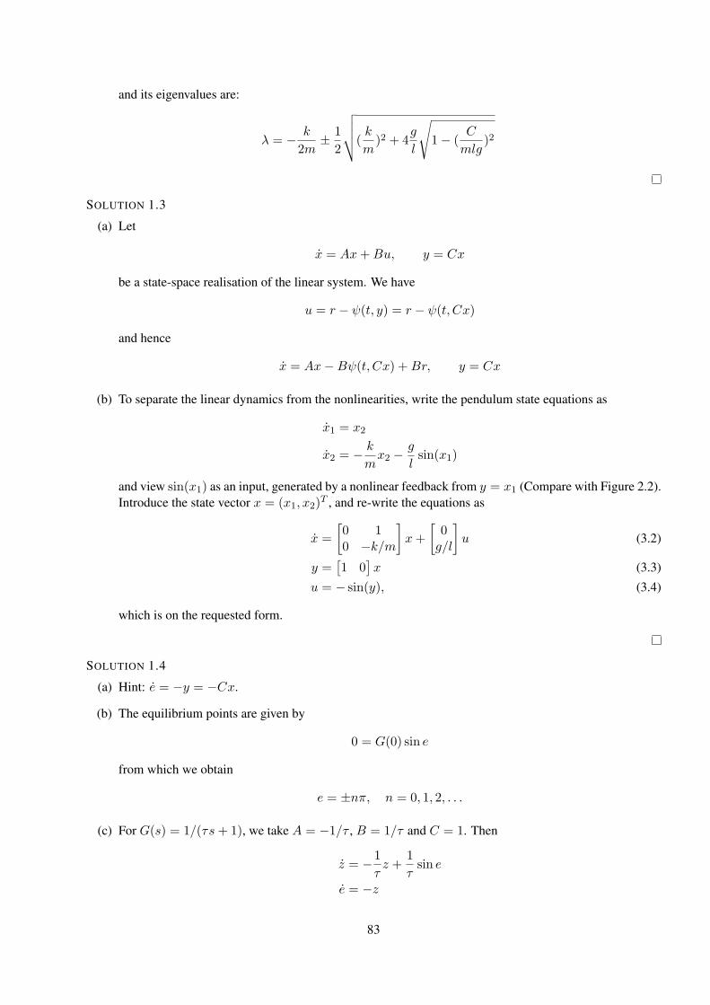
and its eigenvalues are:
λ = − k
2m± 1
2
√√√√(k
m)2 + 4
g
l
√1− (
C
mlg)2
SOLUTION 1.3
(a) Let
x = Ax+Bu, y = Cx
be a state-space realisation of the linear system. We have
u = r − ψ(t, y) = r − ψ(t, Cx)
and hence
x = Ax−Bψ(t, Cx) +Br, y = Cx
(b) To separate the linear dynamics from the nonlinearities, write the pendulum state equations as
x1 = x2
x2 = − k
mx2 −
g
lsin(x1)
and view sin(x1) as an input, generated by a nonlinear feedback from y = x1 (Compare with Figure 2.2).Introduce the state vector x = (x1, x2)
T , and re-write the equations as
x =
[0 10 −k/m
]x+
[0g/l
]u (3.2)
y =[1 0
]x (3.3)
u = − sin(y), (3.4)
which is on the requested form.
SOLUTION 1.4
(a) Hint: e = −y = −Cx.
(b) The equilibrium points are given by
0 = G(0) sin e
from which we obtain
e = ±nπ, n = 0, 1, 2, . . .
(c) For G(s) = 1/(τs+ 1), we take A = −1/τ , B = 1/τ and C = 1. Then
z = −1
τz +
1
τsin e
e = −z
83
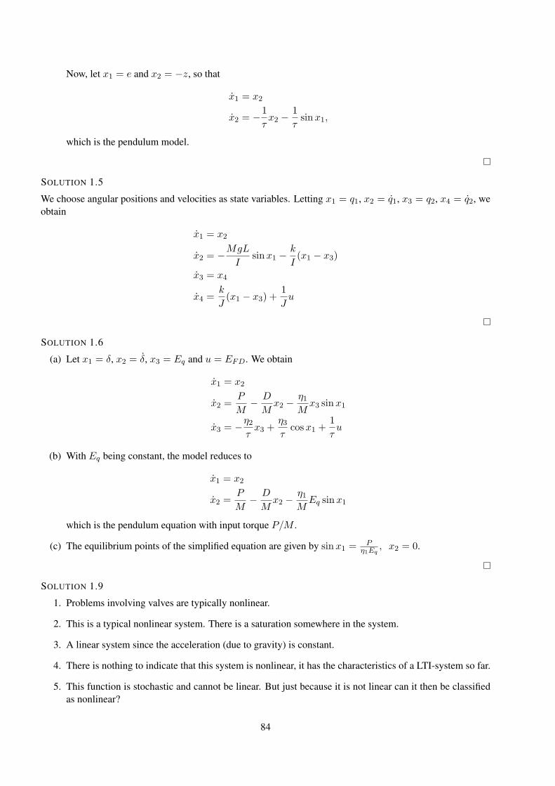
Now, let x1 = e and x2 = −z, so that
x1 = x2
x2 = −1
τx2 −
1
τsinx1,
which is the pendulum model.
SOLUTION 1.5
We choose angular positions and velocities as state variables. Letting x1 = q1, x2 = q1, x3 = q2, x4 = q2, weobtain
x1 = x2
x2 = −MgL
Isinx1 −
k
I(x1 − x3)
x3 = x4
x4 =k
J(x1 − x3) +
1
Ju
SOLUTION 1.6
(a) Let x1 = δ, x2 = δ, x3 = Eq and u = EFD. We obtain
x1 = x2
x2 =P
M− D
Mx2 −
η1Mx3 sinx1
x3 = −η2τx3 +
η3τ
cosx1 +1
τu
(b) With Eq being constant, the model reduces to
x1 = x2
x2 =P
M− D
Mx2 −
η1MEq sinx1
which is the pendulum equation with input torque P/M .
(c) The equilibrium points of the simplified equation are given by sinx1 =P
η1Eq, x2 = 0.
SOLUTION 1.9
1. Problems involving valves are typically nonlinear.
2. This is a typical nonlinear system. There is a saturation somewhere in the system.
3. A linear system since the acceleration (due to gravity) is constant.
4. There is nothing to indicate that this system is nonlinear, it has the characteristics of a LTI-system so far.
5. This function is stochastic and cannot be linear. But just because it is not linear can it then be classifiedas nonlinear?
84

6. The control system for JAS 39 Gripen consists of 50 different linear controllers between which the systemswitches around depending on the operating conditions. The airplane itself is highly nonlinear.
7. This is a nonlinear system. It can only take on two different values, on and off.
SOLUTION 1.10
(a) The system x = f(x) = xu(x) is locally asymptotically stable at x = 0 if
df
dx
∣∣∣∣x=0
= u(0) < 0
(b) u = kx gives x = kx2. If k > 0 then x → ∞ for x(0) > 0 and if k < 0 then x → −∞ for x(0) < 0;hence the system is unstable. For k = 0, we have the equation x = 0 which is not asymptotically stable.
(c) k1 = 0 and k2 < 0 (e.g., k2 = −1) gives x = k2x, which is (globally) asymptotically stable.
(d) The Lyapunov function V (x) = x2/2 can be used to prove that x = −x3 is globally asymptoticallystable.
(e) Follows from the feedback system
x = Ax+Bu
y = Cx
u = ∆y
3.2 Solutions to Computer exercise: Simulation
SOLUTION 2.1
See Lecture 2 for some hints.
SOLUTION 2.2
Blank
SOLUTION 2.2
Blank
SOLUTION 2.3
Blank
SOLUTION 2.4
Blank
SOLUTION 2.5
Plot only one variable, e.g., x1.
85
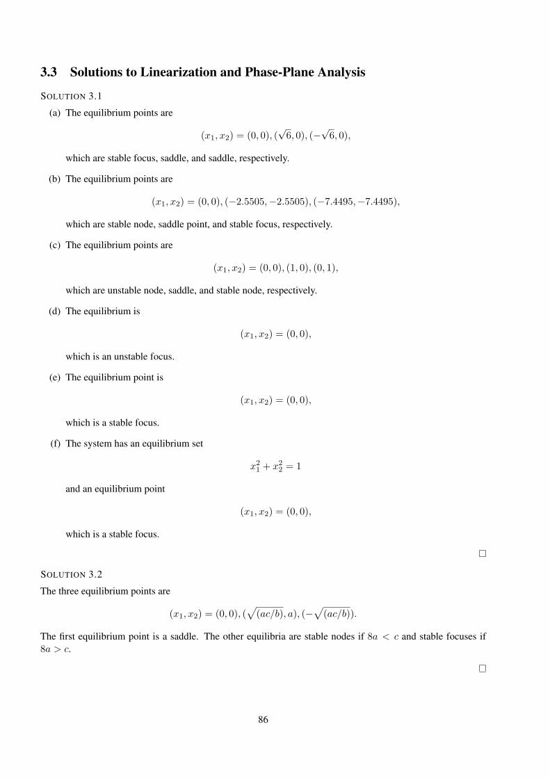
3.3 Solutions to Linearization and Phase-Plane Analysis
SOLUTION 3.1
(a) The equilibrium points are
(x1, x2) = (0, 0), (√6, 0), (−
√6, 0),
which are stable focus, saddle, and saddle, respectively.
(b) The equilibrium points are
(x1, x2) = (0, 0), (−2.5505,−2.5505), (−7.4495,−7.4495),
which are stable node, saddle point, and stable focus, respectively.
(c) The equilibrium points are
(x1, x2) = (0, 0), (1, 0), (0, 1),
which are unstable node, saddle, and stable node, respectively.
(d) The equilibrium is
(x1, x2) = (0, 0),
which is an unstable focus.
(e) The equilibrium point is
(x1, x2) = (0, 0),
which is a stable focus.
(f) The system has an equilibrium set
x21 + x22 = 1
and an equilibrium point
(x1, x2) = (0, 0),
which is a stable focus.
SOLUTION 3.2
The three equilibrium points are
(x1, x2) = (0, 0), (√
(ac/b), a), (−√(ac/b)).
The first equilibrium point is a saddle. The other equilibria are stable nodes if 8a < c and stable focuses if8a > c.
86
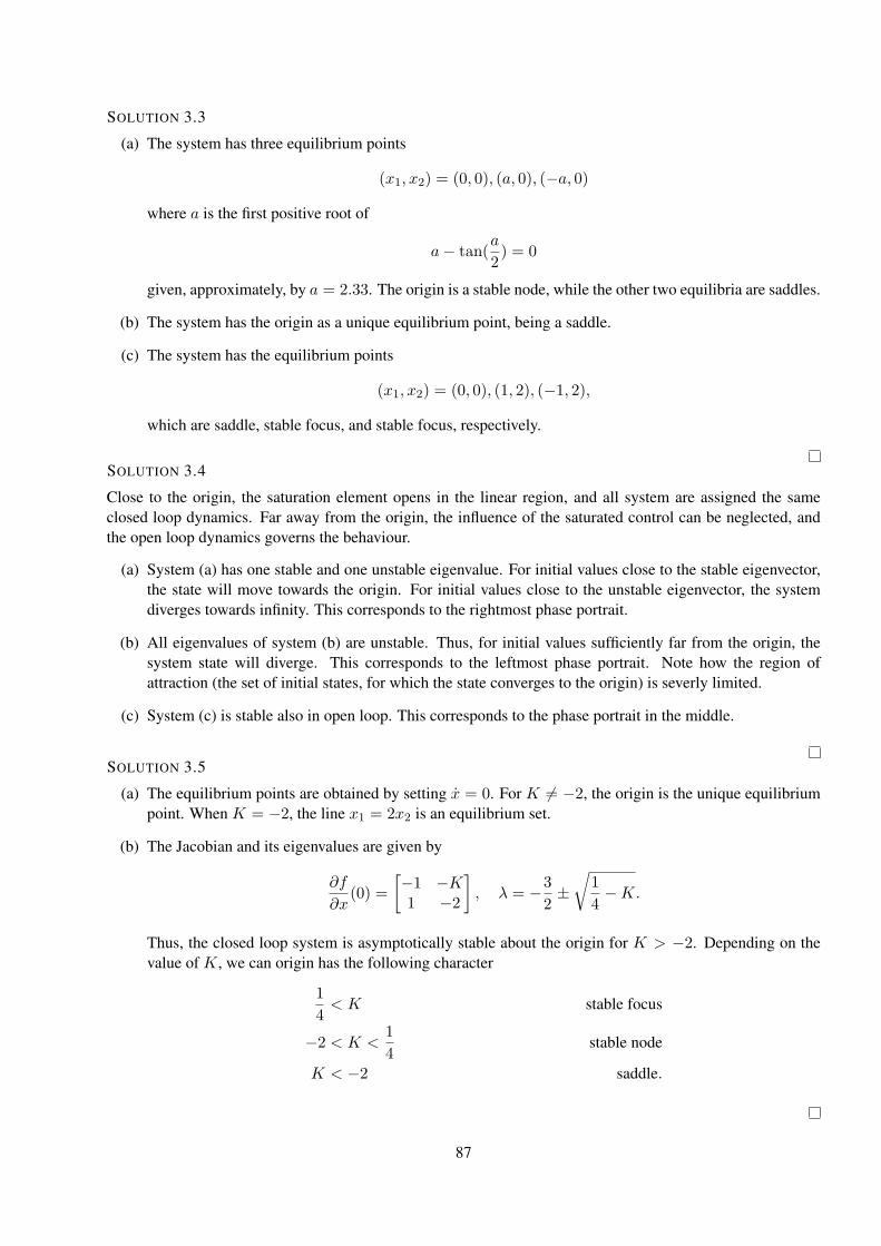
SOLUTION 3.3
(a) The system has three equilibrium points
(x1, x2) = (0, 0), (a, 0), (−a, 0)
where a is the first positive root of
a− tan(a
2) = 0
given, approximately, by a = 2.33. The origin is a stable node, while the other two equilibria are saddles.
(b) The system has the origin as a unique equilibrium point, being a saddle.
(c) The system has the equilibrium points
(x1, x2) = (0, 0), (1, 2), (−1, 2),
which are saddle, stable focus, and stable focus, respectively.
SOLUTION 3.4
Close to the origin, the saturation element opens in the linear region, and all system are assigned the sameclosed loop dynamics. Far away from the origin, the influence of the saturated control can be neglected, andthe open loop dynamics governs the behaviour.
(a) System (a) has one stable and one unstable eigenvalue. For initial values close to the stable eigenvector,the state will move towards the origin. For initial values close to the unstable eigenvector, the systemdiverges towards infinity. This corresponds to the rightmost phase portrait.
(b) All eigenvalues of system (b) are unstable. Thus, for initial values sufficiently far from the origin, thesystem state will diverge. This corresponds to the leftmost phase portrait. Note how the region ofattraction (the set of initial states, for which the state converges to the origin) is severly limited.
(c) System (c) is stable also in open loop. This corresponds to the phase portrait in the middle.
SOLUTION 3.5
(a) The equilibrium points are obtained by setting x = 0. For K 6= −2, the origin is the unique equilibriumpoint. When K = −2, the line x1 = 2x2 is an equilibrium set.
(b) The Jacobian and its eigenvalues are given by
∂f
∂x(0) =
[−1 −K1 −2
], λ = −3
2±√
1
4−K.
Thus, the closed loop system is asymptotically stable about the origin for K > −2. Depending on thevalue of K, we can origin has the following character
1
4< K stable focus
−2 < K <1
4stable node
K < −2 saddle.
87
SOLUTION 3.6
The equilibria are given by sinx01 =P
ηEq, x02 = 0. The characteristic equation for the lineraisation becomes
λ2 + αλ+ β = 0,
where α = DM > 0 and β =
ηEq
M cosx01. Depending on α, β the equilibria are stable focus, stable nodes orsaddle points.
SOLUTION 3.7
˙x = A(t)x, where
A(t) =
(−2 sin2(t) 1− sin(2t)−1− sin(2t) −2 cos2(t)
).
SOLUTION 3.8
7
5¨x = g cos(φ0)φ+
2r
5¨φ
SOLUTION 3.9
Using the identitiy
(sin t)3 =3
4sin t− 1
4sin 3t
we see that u0(t) = sin (3t), y0(t) = sin t is a nominal solution. The linearisation is given by
¨y + 4 sin2 t · y = −1
3u.
SOLUTION 3.10
Introduce f through the equation θ = f(θ, θ, β, β) and let c1, c2, c3 denote the (positive) constants in f . Lin-earizing f around θ = β = β = 0 gives
f(θ, θ, β, β) ≈ ∂f
∂θθ +
∂f
∂θθ +
∂f
∂ββ +
∂f
∂ββ
= c1θ + c2β + c3β
where β = u. Hence, the linearized system is given by
θ = c1θ + c2β + c3u.
It follows that in the Laplace domain
s2θ = c1θ + c2β + c3u = c1θ + (c2/s+ c3)u
and thusG(s) =
c3s+ c2s(s2 − c1)
.
The poles are located in 0,±√c1 and the zero in −c2/c3. The bicycle is, as expected, unstable.
88
SOLUTION 3.11
(a) With x = (θ, θ, φ, φ)T , we have if sin θ 6= 0,
x =
x2x24 sinx1 cosx1 − sinx1
x4−2x2x4 cosx1/ sinx1
(b) Setting all derivatives in the original equation equal to zero, yields sin θ = 0. Hence, the equilibria aredetermined by θk = kπ with φ taking any value. (Note that the equilibria cannot be obtained directlyfrom the first-order form in (a).)
(c) The solution (θ(t), φ(t)) = (π/3, t√2) fulfills the first pendulum equation, since
−2 sinπ/3 cosπ/3 + sinπ/3 = 0
The second equation is also satisfied.
(d) Denote the first pendulum equation by f1(z) = 0 and the second by f2(z) = 0 where z = (θ, θ, θ, φ, φ, φ)T .To linearize these equations, we write
0 = f1(z(t)) = f1(z0(t) + δz(t)) ≈ f1(z
0(t)) +df1dz
∣∣∣∣z=z0(t)
δz(t)
=∂f1∂z1
∣∣∣∣z=z0(t)
δz1(t) + · · ·+ ∂f1∂z6
∣∣∣∣z=z0(t)
δz6(t)
and similar for f2. Deriving the partial derivatives and using the definition of z (δz1 = δθ etc.), we get
3
2δθ + δθ −
√3
2δφ = 0
√2δθ +
√3
2δφ = 0
89
3.4 Solutions to Lyapunov Stability
SOLUTION 4.1
(a) Linearization about the system around the origin yields
A =∂f
∂x= 3ax2
Thus, at the origin we have A = 0. Since the linearization has one eigenvalue on the imaginary axis,linearization fails to determine stability of the origin.
(b) V (0) = 0, V (x) 6= 0 for x 6= 0, and V (x) → ∞ as x → ∞. Thus, V (x) satisfies the conditionsfor being a Lyapunov function candidate. Its time derivative is
V (x) =∂V
∂xf(x) = 4ax6 (3.5)
which is negative definite for a < 0, and positive definite for a > 0. The desired results now followfrom Lyapunov’s stability and instability theorems.
(c) For a = 0, the system is linear and given by
x = 0
The system has solutions x(t) = x0 for all t. Thus, the system is stable. A similar conclusion canbe drawn from the Lyapunov function used in (b).
SOLUTION 4.2
(a) We use the pendulum’s total energy
V (x) = gl(1− cos(x1)) +l2
2x22
as Lyapunov function. We see that V is positive, and compute the time derivative
dV (x)
dt=∑
i
∂V
∂xixi = gl sin(x1)x2 + x2(−gl sin(x1)) = 0
From Lyapunov’s theorem, we conclude that the origin is a stable equilibrium point. Since V (x) = 0,we can also conclude that the origin is not asymptotically stable; trajectories starting at a level surfaceV (x) = c, remain on this surface for all future times.
(b) For k 6= 0, using V (x) as above, similar calculations give
dV (x)
dt= −kl
2
mx22
V (x) is negative semidefinite. It is not negative definite because V (x) = 0 for x2 = 0. In other wordsV (x) = 0 along the x1 axis.
Now, consider a modified Lyapunov function
V (x) =g
l(1− cos(x1)) + xTPx
90
for some positive definite matrix P . In order for P to be positive definite, the elements of P must satisfy
p11 > 0; p22 > 0; p11p22 − p212 > 0
The derivative V (x) is given by
V (x) =g
l(1− p22)x2 sinx1 −
g
lp12x1 sinx1+
+ (p11 − p12k
m)x1x2 + (p12 − p22
k
m)x22
We now want to choose p11, p12 and p22 such that V (x) is negative definite. Since the cross termsx1 sinx1 and x1x2 are sign indefinite, we cancel them out by letting p22 = 1, p11 = p12k/m. With thesechoices, p12 must satsify 0 < p12 < k/m. We let p12 = 0.5k/m, and obtain
V (x) = −1
2
g
l
k
mx1 sinx1 −
1
2
k
mx22.
The term x1 sinx1 > 0 for all 0 < |x1| < π. Within this strip, V (x) is positive definite, and V (x) isnegative definite. We conclude that the origin is asymptotically stable.
SOLUTION 4.3
With V = kx2/2 + x2/2 we get V = −dx4 ≤ 0. Since V = 0 only when x = 0 and the system equation thengives x = −kx 6= 0 unless also x = 0, we conclude that x = x = 0 is the only invariant set. The origin isglobally asymptotically stable since the Lyapunov function is radially unbounded.
SOLUTION 4.4
(a) The eigenvalues of A are λ = −1/2± i√3/2.
(b) (i) We have
V (x) = p11x21 + 2p12x1x2 + p22x
22 = (if p11 6= 0)
= p11(x1 +p12p11
x2)2 + (p22 −
p212p11
)x22
If p11 > 0 and p11p22 − p212 > 0, both terms are non-negative. Moreover, V (x) → ∞ as x → ∞,and V (x) = 0⇒ x1 = x2 = 0 (This proves the "if"-part). If the conditions on pij do not hold, it iseasy to find x such that V (x) < 0 (proving the "only if"-part).
(ii) We want to solve[0 1−1 −1
] [p11 p12p12 p22
]+
[p11 p12p12 p22
] [0 −11 −1
]=
[−1 00 −1
]
Reading off the elements, we see that
2p12 = −1
p22 − p11 − p12 = 0
−2p12 − 2p22 = −1
which has the solution p11 = 1.5, p12 = −0.5 and p22 = 1. P is a positive definite matrix.
91
(c) Use the Matlab command lyap(A’,eye(2)).
SOLUTION 4.7
SOLUTION 4.6
(a) The mistake is that V is not really positive definite. The student has forgotten to check that limx→∞ V (x) =∞, which must hold for a positive definite function. In fact,
V (x1, x2) =x21
1 + x21+
1
2x22
so that limx→∞ = 1. Consequently, V is not positive definite.
(b) No, the problem is not that the student was not clever enough to find a Lyapunov function. There is noLyapunov function, since the system is not globally stable. Let’s show this now. In part (a), you mayhave noticed that V = 0 for all x. In other words, V is an “integral” of the motion; the trajectories lie onthe curves of constant value of V , i.e., we have
V (x) =1
2x22 +
x211 + x21
= V (x0) = c
If c > 1 then x(t) cannot change sign, since
x22 = c− x211 + x21
≥ c− 1
In this case, we have |x2| ≥√c− 1. Since x1 = x2, it follows that |x1| → ∞ as t → ∞. Roughly
speaking, if the system starts with more initial stored energy than can possibly be stored as potentialenergy in the spring, the trajectories will diverge.
SOLUTION 4.7
Left blanc
SOLUTION 4.8
Verify that V (0) = 0, V (x) > 0 for x 6= 0 and V (x) → ∞ for ||x|| → ∞. Now,
(a) We have
d
dtV (x1, x2) = 8x1x1 + 4x2x2 + 16x31x1 =
= 8x1x2 + 4x2(−2x1 − 2x2 − 4x31) + 16x31x2 =
= −8x22
Since V (x) ≤ 0, we conclude global stability.
92
(b) The Lyapunov function has V (x) = 0 for x2 = 0. For x2 = 0, we obtain
x2 = −x1(2 + x21).
which implies that if x2 should remain zero, then x1 has also to be zero. The invariance theorem fromthe lectures can now be used to conlclude global asymptotic stability of the origin.
SOLUTION 4.9
(a) For |2x1 + x2| ≤ 1, we have
x =
[0 1−1 −1
]x. (3.6)
The system matrix is as. stable. Hence, the origin is locally asymptotically stable.
(b) We have V (x) > 0 in the first and third quadrant.
V (x) = x1x2 + x1x2 = x21 − x1sat(2x1 + x2) + x22.
Now, let us evaluate V (x) on the strip x1x2 = c and suppose that c > 0 is chosen so large that thesaturation is active, i.e., |2x1 + x2| > 1. By inspection of the dynamics, we see that for sufficientlylarge c, no trajectories can escape from the first quadrant. We can therefore use the following Lyapunovargument. Consider the Lyapunov function derivative
V (x) = x21 − x1 +c2
x21.
If c ≥ 1, V (x) is positive for all x1 ≥ 0. Hence, all trajectories starting in the first quadrant to the rightof the curve x1x2 = c cannot cross the curve. Consequently, they cannot reach the origin.
(c) It follows from (b) that the origin is not globally asymptotically stable.
SOLUTION 4.10
(a) Integration of the equality ddσf(σx) =
∂f∂x (σx) · x gives the equation
f(x) =
∫ 1
0
∂f
∂x(σx) · x dσ.
We get
xTPf(x) + fT (x)Px = xTP
∫ 1
0
∂f
∂x(σx)xdσ +
∫ 1
0xT[∂f
∂x(σx)
]TdσPx
= xT∫ 1
0
P∂f
∂x(σx) +
[∂f
∂x(σx)
]TP
dσx ≤ −xTx
(b) Since P is positive definite, V (x) is clearly positive semidefinite. To show that it is positive definite, weneed to show that f(x) = 0 only when x = 0. But the inequality proved in (a) shows that if f(p) = 0then
0 ≤ −pT p.
93
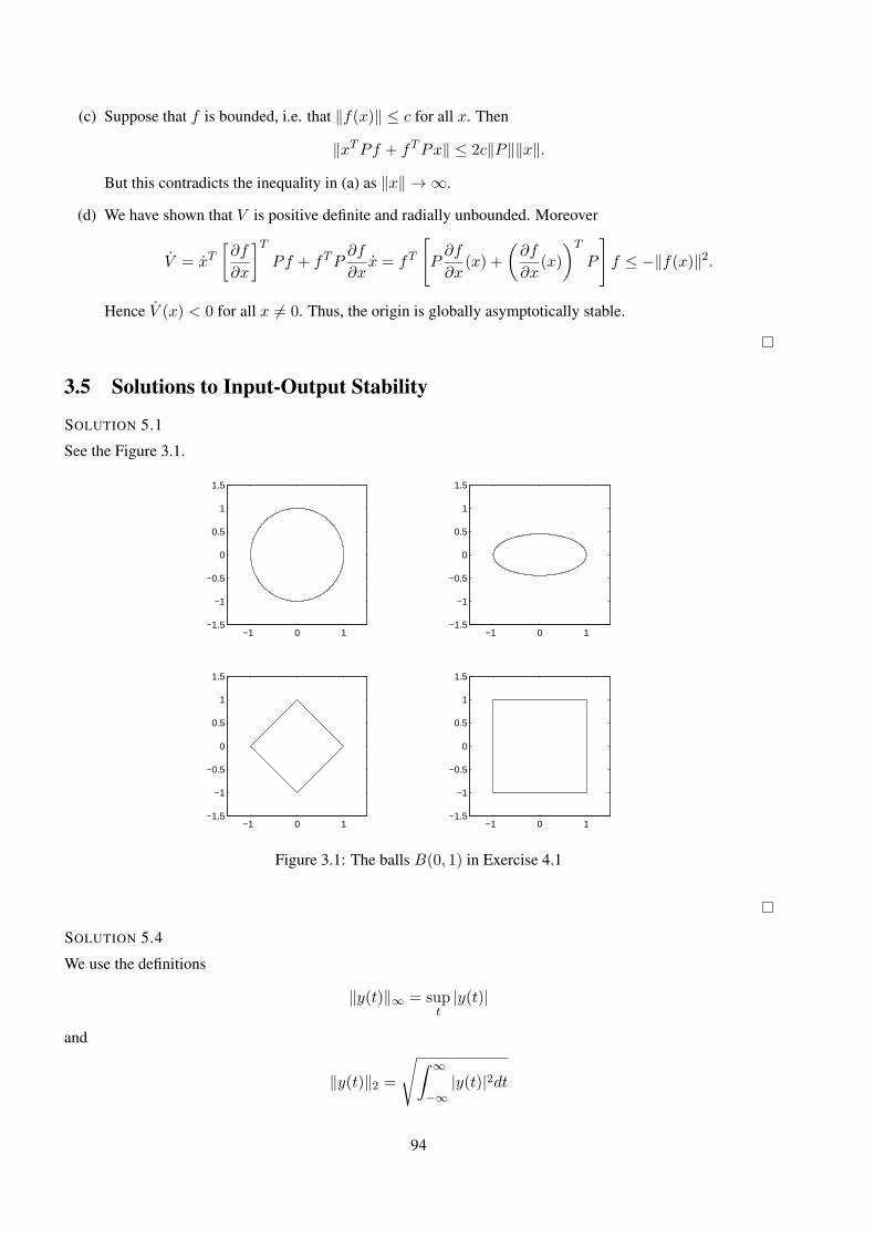
(c) Suppose that f is bounded, i.e. that ‖f(x)‖ ≤ c for all x. Then
‖xTPf + fTPx‖ ≤ 2c‖P‖‖x‖.
But this contradicts the inequality in (a) as ‖x‖ → ∞.
(d) We have shown that V is positive definite and radially unbounded. Moreover
V = xT[∂f
∂x
]TPf + fTP
∂f
∂xx = fT
[P∂f
∂x(x) +
(∂f
∂x(x)
)T
P
]f ≤ −‖f(x)‖2.
Hence V (x) < 0 for all x 6= 0. Thus, the origin is globally asymptotically stable.
3.5 Solutions to Input-Output Stability
SOLUTION 5.1
See the Figure 3.1.
−1 0 1−1.5
−1
−0.5
0
0.5
1
1.5
−1 0 1−1.5
−1
−0.5
0
0.5
1
1.5
−1 0 1−1.5
−1
−0.5
0
0.5
1
1.5
−1 0 1−1.5
−1
−0.5
0
0.5
1
1.5
Figure 3.1: The balls B(0, 1) in Exercise 4.1
SOLUTION 5.4
We use the definitions
‖y(t)‖∞ = supt
|y(t)|
and
‖y(t)‖2 =√∫ ∞
−∞|y(t)|2dt
94
(a)
‖y(t)‖2 =∫ ∞
0a2 sin2(t)dt = ∞
, hence, the signal has infinite energy.
‖y(t)‖∞ = supt
|asin(t)| = |a|
(b)
‖y(t)‖2 =∫ ∞
1
1
t2dt = 1
and
‖y(t)‖∞ = supt>1
|1t| = 1
(c)
‖y(t)‖2 =∫ ∞
0(e−t(1− e−t))2dt =
√3
6
and
‖y(t)‖∞ = supt>0
|e−t(1− e−t)| =
sup0≤x≤1
|x(1− x)| = 1
4
SOLUTION 5.3
‖G‖ = 1, ζ >1√2
since no resonance peak, and
‖G‖ =1
2ζ√
1− ζ2, 0 < ζ <
1√2,
and in this case there is a resonance peak.
SOLUTION 5.4
Note that the requirement that the block ψ(y) should be static is not a restriction for the Small Gain Theoremand the Passivity Theorem, since they can also cope with dynamic nonlinearities. For simplicity, we will onlyconsider the case when the linear system is asymptotically stable.
(a) What are the restrictions that we must impose on the nonlinearities so that we can apply the variousstability theorems?
95
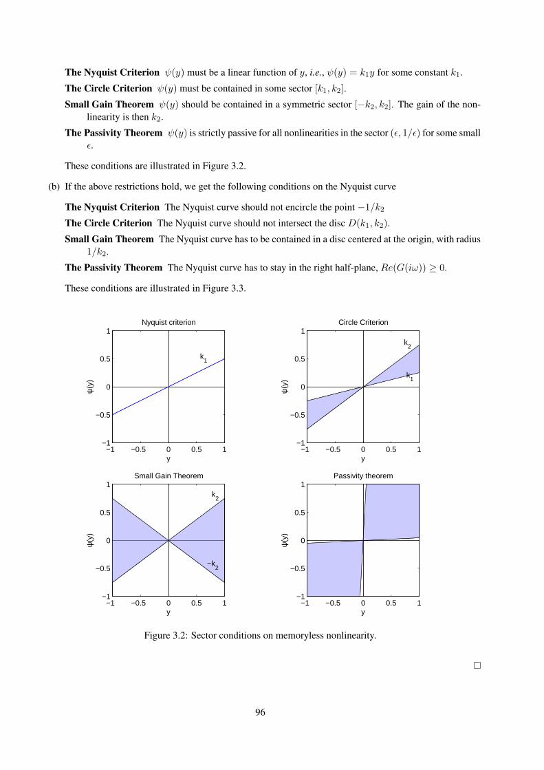
The Nyquist Criterion ψ(y) must be a linear function of y, i.e., ψ(y) = k1y for some constant k1.
The Circle Criterion ψ(y) must be contained in some sector [k1, k2].
Small Gain Theorem ψ(y) should be contained in a symmetric sector [−k2, k2]. The gain of the non-linearity is then k2.
The Passivity Theorem ψ(y) is strictly passive for all nonlinearities in the sector (ǫ, 1/ǫ) for some smallǫ.
These conditions are illustrated in Figure 3.2.
(b) If the above restrictions hold, we get the following conditions on the Nyquist curve
The Nyquist Criterion The Nyquist curve should not encircle the point −1/k2
The Circle Criterion The Nyquist curve should not intersect the disc D(k1, k2).
Small Gain Theorem The Nyquist curve has to be contained in a disc centered at the origin, with radius1/k2.
The Passivity Theorem The Nyquist curve has to stay in the right half-plane, Re(G(iω)) ≥ 0.
These conditions are illustrated in Figure 3.3.
−1 −0.5 0 0.5 1−1
−0.5
0
0.5
1Nyquist criterion
y
ψ(y
)
k1
−1 −0.5 0 0.5 1−1
−0.5
0
0.5
1Circle Criterion
y
ψ(y
)
k1
k2
−1 −0.5 0 0.5 1−1
−0.5
0
0.5
1Small Gain Theorem
y
ψ(y
)
k2
−k2
−1 −0.5 0 0.5 1−1
−0.5
0
0.5
1Passivity theorem
y
ψ(y
)
Figure 3.2: Sector conditions on memoryless nonlinearity.
96
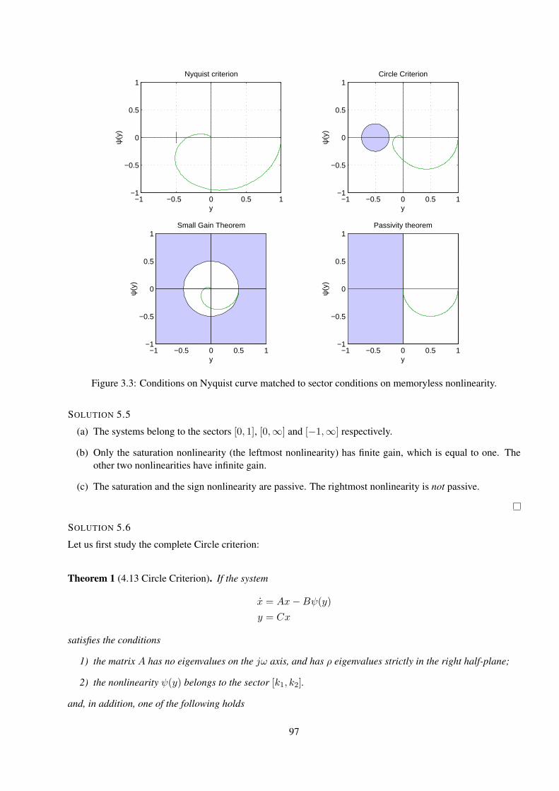
−1 −0.5 0 0.5 1−1
−0.5
0
0.5
1Nyquist criterion
y
ψ(y
)
−1 −0.5 0 0.5 1−1
−0.5
0
0.5
1Circle Criterion
y
ψ(y
)
−1 −0.5 0 0.5 1−1
−0.5
0
0.5
1Small Gain Theorem
y
ψ(y
)
−1 −0.5 0 0.5 1−1
−0.5
0
0.5
1Passivity theorem
y
ψ(y
)
Figure 3.3: Conditions on Nyquist curve matched to sector conditions on memoryless nonlinearity.
SOLUTION 5.5
(a) The systems belong to the sectors [0, 1], [0,∞] and [−1,∞] respectively.
(b) Only the saturation nonlinearity (the leftmost nonlinearity) has finite gain, which is equal to one. Theother two nonlinearities have infinite gain.
(c) The saturation and the sign nonlinearity are passive. The rightmost nonlinearity is not passive.
SOLUTION 5.6
Let us first study the complete Circle criterion:
Theorem 1 (4.13 Circle Criterion). If the system
x = Ax−Bψ(y)
y = Cx
satisfies the conditions
1) the matrix A has no eigenvalues on the jω axis, and has ρ eigenvalues strictly in the right half-plane;
2) the nonlinearity ψ(y) belongs to the sector [k1, k2].
and, in addition, one of the following holds
97
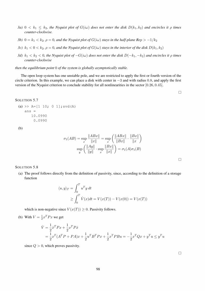
3a) 0 < k1 ≤ k2, the Nyquist plot of G(iω) does not enter the disk D(k1, k2) and encircles it ρ times
counter-clockwise.
3b) 0 = k1 < k2, ρ = 0, and the Nyquist plot of G(iω) stays in the half-plane Rep > −1/k2
3c) k1 < 0 < k2, ρ = 0, and the Nyquist plot of G(iω) stays in the interior of the disk D(k1, k2)
3d) k1 < k2 < 0, the Nyquist plot of −G(iω) does not enter the disk D(−k1,−k2) and encircles it ρ times
counter-clockwise
then the equilibrium point 0 of the system is globally asymptotically stable.
The open loop system has one unstable pole, and we are restricted to apply the first or fourth version of thecircle criterion. In this example, we can place a disk with center in −3 and with radius 0.8, and apply the firstversion of the Nyquist criterion to conclude stability for all nonlinearities in the sector [0.26, 0.45].
SOLUTION 5.7
(a) >> A=[1 10; 0 1];svd(A)
ans =
10.0990
0.0990
(b)
σ1(AB) = supx
‖ABx‖‖x‖ = sup
x
(‖ABx‖‖Bx‖ · ‖Bx‖‖x
)
supy
(‖Ay‖‖y‖ · sup
x
‖Bx‖‖x‖
)= σ1(A)σ1(B)
SOLUTION 5.8
(a) The proof follows directly from the definition of passivity, since, according to the definition of a storagefunction
〈u, y〉T =
∫ T
0uT y dt
≥∫ T
0V (x)dt = V (x(T ))− V (x(0)) = V (x(T ))
which is non-negative since V (x(T )) ≥ 0. Passivity follows.
(b) With V = 12x
TPx we get
V =1
2xTPx+
1
2xTPx
=1
2xT (ATP + PA)x+
1
2uTBTPx+
1
2xTPBu = −1
2xTQx+ yTu ≤ yTu
since Q > 0, which proves passivity.
98
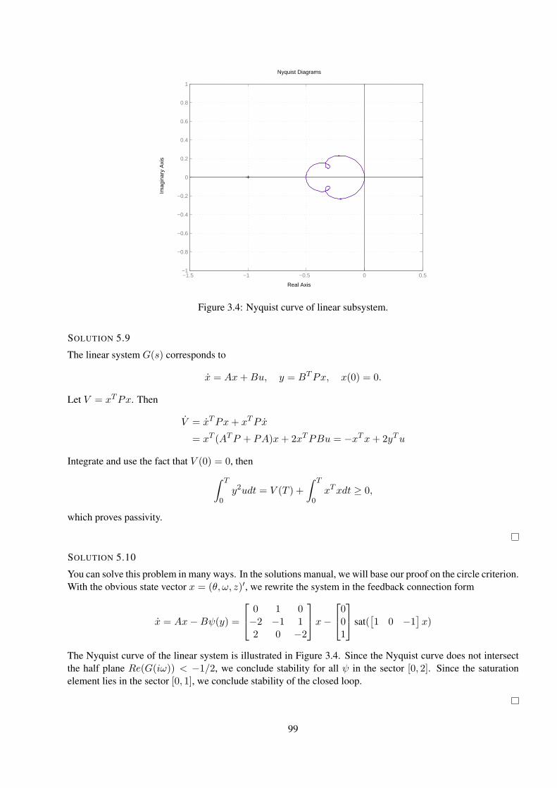
Real Axis
Imag
inar
y A
xis
Nyquist Diagrams
−1.5 −1 −0.5 0 0.5−1
−0.8
−0.6
−0.4
−0.2
0
0.2
0.4
0.6
0.8
1
Figure 3.4: Nyquist curve of linear subsystem.
SOLUTION 5.9
The linear system G(s) corresponds to
x = Ax+Bu, y = BTPx, x(0) = 0.
Let V = xTPx. Then
V = xTPx+ xTPx
= xT (ATP + PA)x+ 2xTPBu = −xTx+ 2yTu
Integrate and use the fact that V (0) = 0, then
∫ T
0y2udt = V (T ) +
∫ T
0xTxdt ≥ 0,
which proves passivity.
SOLUTION 5.10
You can solve this problem in many ways. In the solutions manual, we will base our proof on the circle criterion.With the obvious state vector x = (θ, ω, z)′, we rewrite the system in the feedback connection form
x = Ax−Bψ(y) =
0 1 0−2 −1 12 0 −2
x−
001
sat(
[1 0 −1
]x)
The Nyquist curve of the linear system is illustrated in Figure 3.4. Since the Nyquist curve does not intersectthe half plane Re(G(iω)) < −1/2, we conclude stability for all ψ in the sector [0, 2]. Since the saturationelement lies in the sector [0, 1], we conclude stability of the closed loop.
99
SOLUTION 5.11
(a) We have
〈y, u〉 =∫ T
0y(t)u(t)dt =
=
∫ T
0u(t)uc(t)H(u(t)uc(t))dt =
=
∫ T
0w(t)H(w(t))dt = 〈w,H(w)〉
where w = ucu. Since H is passive, the result follows.
(b) We will only consider the case where θ0 = 0. The case θ0 is a little tricker, and the discussion about thiscase is postponed to the course in Adaptive Control.
If θ0 = 0, the system equations read
e(t) = G(p)θuc(t)
θ(t) = −γuc(t)e(t)
In light of exercise (a), we can identify the second equation modeling the signal w(t) = uc(t)e(t) sentinto an integrator with gain γ and postmultiplied by uc (See the lecture slides for an illustration). Thissystem is passive, and interconnected in a negative feedback loop with the strictly passive system G.Stability now follows from the passivity theorem.
SOLUTION 5.12
(a) For simplicity we include ∆ in the nonlinearity, and thus consider G(s) = 1/[s(s+1)] in feedback withf(y) = ∆K arctan(y). Note that Re ˆG(iω) = −1/(1 + ω2) > −1 and that f(·) is bounded by thesector [0,∆K]. The Circle Criterion now gives BIBO stability for ∆K < 1.
(b) Small Gain Theorem is not applicable since the gain of 1/s is infinite.
SOLUTION 5.13
(a) True. Suppose x and x are two equilibria. A trajectory that starts in either point, stays there forever sincef(x) = f(x) = 0.
(b) False. As a counter example, take for instance the system from Lecture 3:
x1 = x1 − x2 − x1(x21 + x22)
x2 = x1 + x2 − x2(x21 + x22).
(c) True. Follows from Lyapunov’s linearization method (Lectures 3 and 4).
(d) True. For example,
x =
(−1 00 −1
)x
100
(e) True. Suppose it was not true. Consider a solution of x = f(x) that starts in x0 6= 0 and ends atx(T ) = x1 = 0. Then, x = −f(x) has a solution that starts in x1 = 0 and ends at x0 6= 0. However,x = −f(x) also has the solution x(t) = 0 for all t ∈ (0, T ), since x = 0. This is a contradiction to thatx = −f(x) has a unique solution, which holds because f is C1 (Lecture 1). Hence, the statement in theproblem must be true.
SOLUTION 5.14
(a) The linearization is given by
A =df
dx(0, 0) =
(0 −11 −1
)
with characteristic polynomial s2 + s+ 1. Hence, the system is asymptotically stable.
(b)
P =
(3 −1−1 2
)
(c)
V =dV
dxf(x) = 2
(x1 x2
)P
(−x2
x1 + (x21 − 1)x2
)
gives the expression.
(d) c = 4 corresponds to that largest Ωc contained in Π.
SOLUTION 5.15
1. True
2. False, We get no information about BIBO-stability from that particular methods (if they are not fulfilled).We have to try some other methods.
3. True, only one of them has to be fulfilled.
4. False, One of them has to be strictly passive to get a BIBO-stable system.
5. True
6. True
101
3.6 Solutions to Describing Function Analysis
SOLUTION 6.1
Let the input to the relay be
u(t) = A sin(ωt) = A sin(φ)
The ouput of the relay is then
y(φ) =
−H 0 < φ < φ0
H φ0 < φ < π + φ0
−H π + φ0 < φ < 2π
where φ0 = arcsin(D/A). We get
a1 =1
π
∫ 2π
0y(φ) cos(φ)dφ
=1
π
∫ φ0
0(−H) cos(φ)dφ+
1
π
∫ π+φ0
φ0
H cos(φ)dφ+1
π
∫ 2π
π+φ0
(−H) cos(φ)dφ
= −4H
πsin(φ0)
and
b1 =1
π
∫ 2π
0y(φ) sin(φ)dφ
=1
π
∫ φ0
0(−H) sin(φ)dφ+
1
π
∫ π+φ0
φ0
H sin(φ)dφ+1
π
∫ 2π
π+φ0
(−H) sin(φ)dφ
=4H
πcos(φ0)
We obtain
N(A) =4H
πA(cos(φ0)− i sin(φ0))
The identity cos(z) =√1− sin2(z) gives the desired result.
SOLUTION 6.2
Use the interpretation of describing function as “equivalent gain”. We have 1-b, 2-c, 3-a, 4-d.
SOLUTION 6.3
Denote the nonlinearity by f . For memoryless, static nonlinearities, the describing function does not dependon ω, and the describing function in Slotine and Li reduces to
N(A) =b1(A) + ia1(A)
A
where a1 and b1 can be computed as
a1 =1
π
∫ 2π
0f(A sin(φ)) cos(φ) dφ (3.7)
b1 =1
π
∫ 2π
0f(A sin(φ)) sin(φ) dφ. (3.8)
102
(a) First, we notice that the saturation is a odd function, which implies that a1 = 0. In order to simplify thecomputations of b1, we set H = 1 and note that the saturation can be described as
f(A sin(φ)) =
A/D sin(φ) 0 ≤ φ ≤ φl
1 φl < φ < π/2
Here, φl = arcsin(D/A) denotes the value of φ where so that f saturates. Now,
b1 =1
π
∫ 2π
0u(φ) sin(φ)dφ =
=4
π
∫ π/2
0u(φ) sin(φ)dφ =
=4
π
(∫ φl
0A/D sin2(φ)dφ+
∫ π/2
φl
sin(φ)dφ
)=
=4
π
(∫ φl
0A/(2D)(1− cos(2φ))dφ+
∫ π/2
φl
sin(φ)dφ
)=
=4
π(A/(2D)(φl − sin(φl) cos(φl)) + cos(φl)) =
=2A
Dπ
(φl +
D
Acos(φl)
)
Thus, the describing function for the normalized saturation is
N(A) =2
Dπ(φl +
D
Acos(φl))
Now, using the calculation rule Nαf (A) = αNf (A), we find that for the saturation under considerationwe have
N(A) =2H
Dπ(φl +
D
Acos(φl))
(b) We see that the nonlinearity is a superposition of a linear function
g(e) =H
De
and the nonlinearity −f(e) with f(e) as in (a). Using the fact that a linear function g(e) = ke hasdescribing function N(A) = k, and the superposition rule Nf+g(A) = Nf (A) +Ng(A), we find
N(A) =H
D
(1− 2
π
φl +
D
Acos(φl)
)
(c) Noting that this nonlinearity can be written as the sum of the two nonlinearities in (a) and (b), we arriveat the describing function
N(A) =2(α− β)
π
(φl +
D
Acos(φl)
)+ β.
103
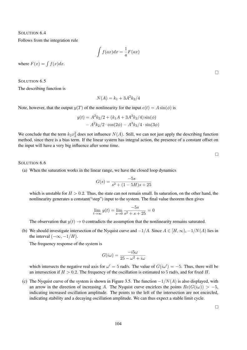
SOLUTION 6.4
Follows from the integration rule∫f(ax)dx =
1
aF (ax)
where F (x) =∫f(x)dx.
SOLUTION 6.5
The describing function is
N(A) = k1 + 3A2k2/4
Note, however, that the output y(T ) of the nonlinearity for the input e(t) = A sin(φ) is
y(t) = A2k2/2 + (k1A+ 3A3k2/4) sin(φ)
−A2k2/2 · cos(2φ)−A3k3/4 · sin(3φ)
We conclude that the term k2x22 does not influence N(A). Still, we can not just apply the describing function
method, since there is a bias term. If the linear system has integral action, the presence of a constant offset onthe input will have a very big influence after some time.
SOLUTION 6.6
(a) When the saturation works in the linear range, we have the closed loop dynamics
G(s) =−5s
s2 + (1− 5H)s+ 25
which is unstable for H > 0.2. Thus, the state can not remain small. In saturation, on the other hand, thenonlinearity generates a constant(“step”) input to the system. The final value theorem then gives
limt→∞
y(t) = lims→0
−5s
s2 + s+ 25= 0
The observation that y(t) → 0 contradicts the assumption that the nonlinearity remains saturated.
(b) We should investigate intersection of the Nyquist curve and −1/A. Since A ∈ [H,∞), −1/N(A) lies inthe interval (−∞,−1/H).
The frequency response of the system is
G(iω) =−i5ω
25− ω2 + iω
which intersects the negative real axis for ω′ = 5 rad/s. The value of G(iω′) = −5. Thus, there will bean intersection if H > 0.2. The frequency of the oscillation is estimated to 5 rad/s, and for fixed H .
(c) The Nyquist curve of the system is shown in Figure 3.5. The function −1/N(A) is also displayed, withan arrow in the direction of increasing A. The Nyquist curve encirlces the points Re(G(iω)) > −5,indicating increased oscillation amplitude. The points to the left of the intersection are not encircled,indicating stability and a decaying oscillation amplitude. We can thus expect a stable limit cycle.
104
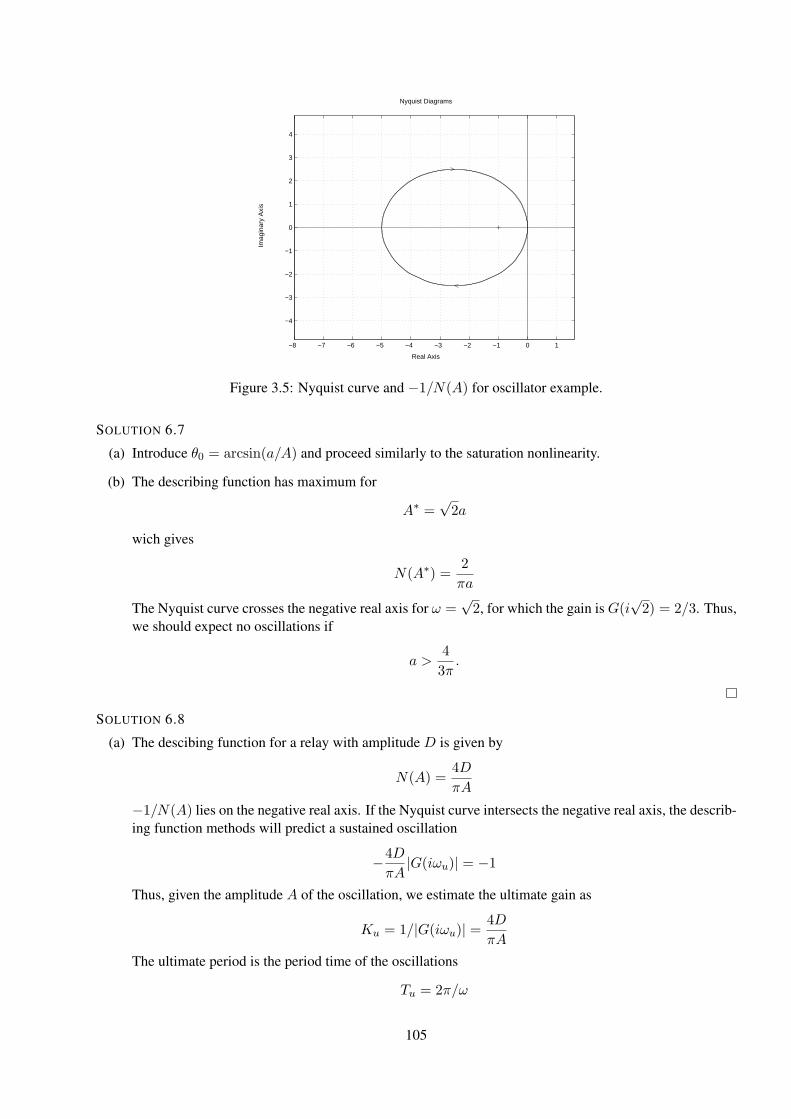
Real Axis
Imag
inar
y A
xis
Nyquist Diagrams
−8 −7 −6 −5 −4 −3 −2 −1 0 1
−4
−3
−2
−1
0
1
2
3
4
Figure 3.5: Nyquist curve and −1/N(A) for oscillator example.
SOLUTION 6.7
(a) Introduce θ0 = arcsin(a/A) and proceed similarly to the saturation nonlinearity.
(b) The describing function has maximum for
A∗ =√2a
wich gives
N(A∗) =2
πa
The Nyquist curve crosses the negative real axis for ω =√2, for which the gain isG(i
√2) = 2/3. Thus,
we should expect no oscillations if
a >4
3π.
SOLUTION 6.8
(a) The descibing function for a relay with amplitude D is given by
N(A) =4D
πA
−1/N(A) lies on the negative real axis. If the Nyquist curve intersects the negative real axis, the describ-ing function methods will predict a sustained oscillation
−4D
πA|G(iωu)| = −1
Thus, given the amplitude A of the oscillation, we estimate the ultimate gain as
Ku = 1/|G(iωu)| =4D
πA
The ultimate period is the period time of the oscillations
Tu = 2π/ω
105
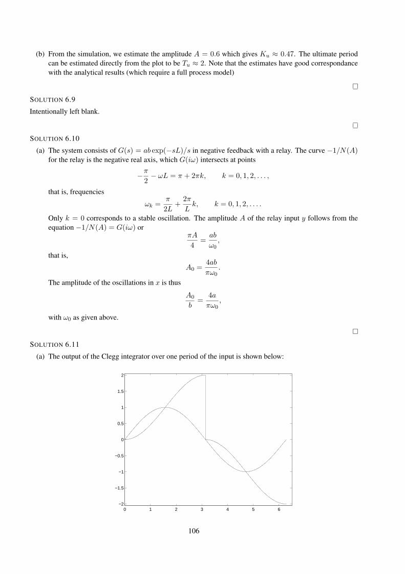
(b) From the simulation, we estimate the amplitude A = 0.6 which gives Ku ≈ 0.47. The ultimate periodcan be estimated directly from the plot to be Tu ≈ 2. Note that the estimates have good correspondancewith the analytical results (which require a full process model)
SOLUTION 6.9
Intentionally left blank.
SOLUTION 6.10
(a) The system consists of G(s) = ab exp(−sL)/s in negative feedback with a relay. The curve −1/N(A)for the relay is the negative real axis, which G(iω) intersects at points
−π2− ωL = π + 2πk, k = 0, 1, 2, . . . ,
that is, frequencies
ωk =π
2L+
2π
Lk, k = 0, 1, 2, . . . .
Only k = 0 corresponds to a stable oscillation. The amplitude A of the relay input y follows from theequation −1/N(A) = G(iω) or
πA
4=ab
ω0,
that is,
A0 =4ab
πω0.
The amplitude of the oscillations in x is thus
A0
b=
4a
πω0,
with ω0 as given above.
SOLUTION 6.11
(a) The output of the Clegg integrator over one period of the input is shown below:
0 1 2 3 4 5 6−2
−1.5
−1
−0.5
0
0.5
1
1.5
2
106
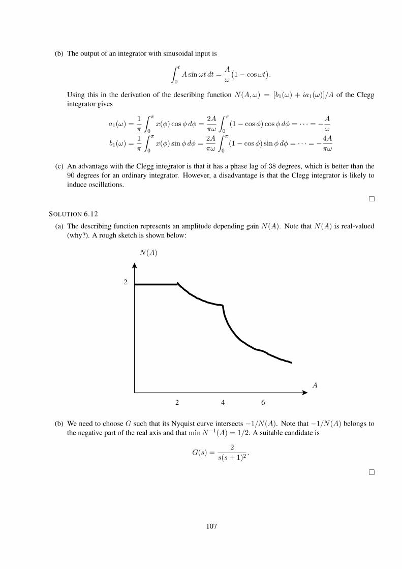
(b) The output of an integrator with sinusoidal input is
∫ t
0A sinωt dt =
A
ω
(1− cosωt
).
Using this in the derivation of the describing function N(A,ω) = [b1(ω) + ia1(ω)]/A of the Cleggintegrator gives
a1(ω) =1
π
∫ π
0x(φ) cosφ dφ =
2A
πω
∫ π
0(1− cosφ) cosφ dφ = · · · = −A
ω
b1(ω) =1
π
∫ π
0x(φ) sinφ dφ =
2A
πω
∫ π
0(1− cosφ) sinφ dφ = · · · = −4A
πω
(c) An advantage with the Clegg integrator is that it has a phase lag of 38 degrees, which is better than the90 degrees for an ordinary integrator. However, a disadvantage is that the Clegg integrator is likely toinduce oscillations.
SOLUTION 6.12
(a) The describing function represents an amplitude depending gain N(A). Note that N(A) is real-valued(why?). A rough sketch is shown below:
2
2 4 6
N(A)
A
(b) We need to choose G such that its Nyquist curve intersects −1/N(A). Note that −1/N(A) belongs tothe negative part of the real axis and that minN−1(A) = 1/2. A suitable candidate is
G(s) =2
s(s+ 1)2.
107
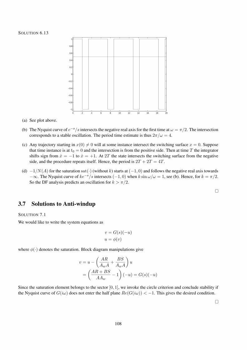
SOLUTION 6.13
0 2 4 6 8 10 12 14 16 18 20
−1
−0.8
−0.6
−0.4
−0.2
0
0.2
0.4
0.6
0.8
1
(a) See plot above.
(b) The Nyquist curve of e−s/s intersects the negative real axis for the first time at ω = π/2. The intersectioncorresponds to a stable oscillation. The period time estimate is thus 2π/ω = 4.
(c) Any trajectory starting in x(0) 6= 0 will at some instance intersect the switching surface x = 0. Supposethat time instance is at t0 = 0 and the intersection is from the positive side. Then at time T the integratorshifts sign from x = −1 to x = +1. At 2T the state intersects the switching surface from the negativeside, and the procedure repeats itself. Hence, the period is 2T + 2T = 4T .
(d) −1/N(A) for the saturation sat(·) (without k) starts at (−1, 0) and follows the negative real axis towards−∞. The Nyquist curve of ke−s/s intersects (−1, 0) when k sinω/ω = 1, see (b). Hence, for k = π/2.So the DF analysis predicts an oscillation for k > π/2.
3.7 Solutions to Anti-windup
SOLUTION 7.1
We would like to write the system equations as
v = G(s)(−u)u = φ(v)
where φ(·) denotes the saturation. Block diagram manipulations give
v = u−(AR
AwA+
BS
AwA
)u
=
(AR+BS
AAw− 1
)(−u) = G(s)(−u)
Since the saturation element belongs to the sector [0, 1], we invoke the circle criterion and conclude stability ifthe Nyquist curve of G(iω) does not enter the half plane Re(G(iω)) < −1. This gives the desired condition.
108
SOLUTION 7.2
(a) Loopgain given by
G0(s) = F (s)G(s) =KcN(sTi + 1 + s2TiTd)(s+ b)
T 2i s
2(s+ 0.1)(s+ bN)
We choose b = 0.1 for simpler calculations. Note, that in reality this will not necessarily be a goodchoice. With this choice, however, the imaginary part of G0(iω) is given by
−KcN(0.1TiN − 1 + ω2TiTd)
ωT 2i (N + ω2)
which is negative for all ω > 0 if N > 10/Ti. Thus, the Nyquist curve of the loopgain is never crossingthe negative real axis and especially not the real axis to the left of −1, and the describing function methodpredicts no autooscillations.
(b) It holds that
U(s) =W (s)[U(s)− U(s)
]− F (s)G(s)U(s)
from which follows that U(s) = −H(s)U(s) with
H(s) =F (s)G(s)−W (s)
1 +W (s)
The describing function methods predicts no autooscillations if the Nyquist curve forH(s) does not crossthe negative real axis to the left of −1. This is equivalent with the Nyquist curve of
1 +H(s) =1 + F (s)G(s)
1 +W (s)
not crossing the negative real axis. We start by calculating the denominator.
1 + F (s)G(s) =s2(s+ 0.1) +Kc(s+ 1/Ti + s2Td)
s2(s+ 0.1)
=(s+ αω0)(s
2 + 2ζω0s+ ω20)
s2(s+ 0.1)
=(s+ 1)(s2 + 0.7s+ 0.25)
s2(s+ 0.1)
This leads to
1 +H(s) =(s+ 1)(s2 + 0.7s+ 0.25)
s(s+ 0.1)(s+ 1/Tt)
If Tt = 1 it holds that
1 +H(s) =s2 + 0.7s+ 0.25
s(s+ 0.1)
Let s = iω. The phase of the denominator is −π/2 for ω = 0 and decreases to −π for ω → ∞. Thephase of the nominator is 0 for ω = 0 and increases to π for ω → ∞. Therefor it holds that the phase of1 + H(iω) is larger than −π for all frequencies ω > 0. Thus, the describing function method predictsno autooscillations. Note that even all values for Tt such that 0 < Tt ≤ 1 are allowed, as the phase of(iω + 1)/(iω + 1/Tt) is positive. Note also that we didn’t take into account values Tt > 1.
(c) The method in (a) does not require to measure or compute the saturated signal, which is an advantage.A drawback is that the amplification of high frequency components increases, which can be a problemespecially in the case of strong measurement noise in the problematic frequency range. The method in(b) does not modify the closed loop systems dynamic if the control signal is not saturated, which is anadvantage. A drawback is that the saturated control signal needs to be measured or calculated.
109
SOLUTION 7.4
Large Tt corresponds to low feedback of the error signal v−u (see the lecture slides for notation). Hence,Tt = 3 corresponds to the largest overshoot in y, Tt = 2 corresponds to the slightly smaller overshootetc. Similarly for u, Tt = 3 corresponds to the curve that is saturated the longest amount of time etc.
SOLUTION 7.5
(a) The upper plots show ysp (solid) and y (dashed). The middle plots show P (solid) and I (dashed). Thelower plots show u (solid) and v (dashed).
From P in the middle plots we see that K ≈ 1.5. From the left plots, it follows that the maximum of
I(t) =K
Ti
∫ t
0[ysp(s)− y(s)] ds
is maxt I(t) ≈ 1 and attained at t ≈ 2. From the upper left plot we have∫ 20 [ysp(s) − y(s)] ds ≈ 1.
Hence, approximately Ti = K = 1.5. From the lower plots we see that the saturation level is equal to0.5.
(b)
G(s) = −(KTt − 1)Tis+KTtTis(Tts+ 1)
(c) With notation from the lectures, the saturation satisfies k1 = 0 and k2 = 1. Note the negative feedback.The Circle Criterion is thus fulfilled if the Nyquist curve of −G is to the right of the line z ∈ C : Re z =−1. Here Re (−G(iω)) = −1/(ω2 + 1), so the criterion is fulfilled. Hence, the closed-loop system isBIBO stable for all K > 1.
3.8 Solutions to Friction, Backlash and Quantization
SOLUTION 8.1
The model is given by
dz
dt= v − |v|
g(v)z (3.9)
F = σ0z + σ1(v)dz
dt+ Fvv (3.10)
(a) For any constant velocity, v, (3.9) converges to the value
z =g(v)
|v| v = g(v)sign(v)
and F therefore converges to
F = σ0g(v)sign(v) + Fvv
110
(b) Consider the storage function V (z) = z2/2. We have
zv = zdz
dt+
|v|g(v)
z2 ≥ zdz
dt= V (t)
and passivity follows from the discussion in (+).
(c) Consider the storage function V (z) = σ0z2. We have
Fv = Fvv2 + (σ1z + σ0z)(z +
|v|g(v)
z) (3.11)
≥ σ1z2 +
|v|g(v)
σ0z2 + (
|v|g(v)
σ1 + σ0)zz (3.12)
Next, we separate out the storage function derivative and make a completion of squares to estimate theadditional terms
Fv ≥ σ0zz + σ1z2 + σ0
|v|g(v)
z2 + σ1|v|g(v)
zz (3.13)
= V + σ1
(z +
|v|2g(v)
z
)2
+
(σ0
|v|g(v)
− σ1
( |v|2g(v)
)2)z2 (3.14)
Since the second term is non-negative, we have
Fv ≥ V
and thus passivity if
σ0 − σ1|v|
4g(v)> 0
This concludes the proof.
111
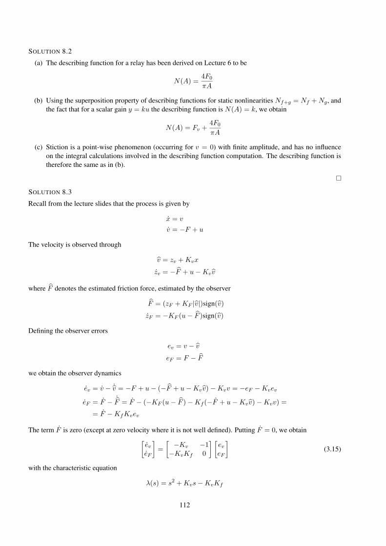
SOLUTION 8.2
(a) The describing function for a relay has been derived on Lecture 6 to be
N(A) =4F0
πA
(b) Using the superposition property of describing functions for static nonlinearities Nf+g = Nf +Ng, andthe fact that for a scalar gain y = ku the describing function is N(A) = k, we obtain
N(A) = Fv +4F0
πA
(c) Stiction is a point-wise phenomenon (occurring for v = 0) with finite amplitude, and has no influenceon the integral calculations involved in the describing function computation. The describing function istherefore the same as in (b).
SOLUTION 8.3
Recall from the lecture slides that the process is given by
x = v
v = −F + u
The velocity is observed through
v = zv +Kvx
zv = −F + u−Kv v
where F denotes the estimated friction force, estimated by the observer
F = (zF +KF |v|)sign(v)
zF = −KF (u− F )sign(v)
Defining the observer errors
ev = v − v
eF = F − F
we obtain the observer dynamics
ev = v − ˙v = −F + u− (−F + u−Kv v)−Kvv = −eF −Kvev
eF = F − ˙F = F − (−KF (u− F )−Kf (−F + u−Kvv)−Kvv) =
= F −KfKvev
The term F is zero (except at zero velocity where it is not well defined). Putting F = 0, we obtain[eveF
]=
[−Kv −1
−KvKf 0
] [eveF
](3.15)
with the characteristic equation
λ(s) = s2 +Kvs−KvKf
112
We conclude that the error dynamics are locally asymptotically stable if
Kv > 0,
−KvKf > 0
which implies the desired conditions.
SOLUTION 8.4
Intentionally left blank.
SOLUTION 8.5
We have
〈u, y〉T =
∫ T
0uy dt =
∫ T
0usat(u) dt ≥ 0
We conclude passivity from to the definition given in the lecture slides.
SOLUTION 8.6
Intentionally left blank.
SOLUTION 8.7
Intentionally left blank.
SOLUTION 8.8
(a) The system is defined by
x = sat(u− x)
y = x+ sat(u− x)
If |u− x| ≤ 1 then y = u. If u− x > 1 then
x = 1
y = x+ 1
and thus x will increase until u− x < 1 so that y = u holds again. Similar for u− x < −1.
SOLUTION 8.9
a) limA→∞ Im N(A) = 0 and limA→∞Re N(A) = 1 then − 1N(A) → −1 as A → ∞. This means that when
the amplitude is large enough the Nyquist curve for G(s) will intersect − 1N(A) in -1. The conclusion is that the
backlash can be neglected.b) If the amplitude is smaller then the size of the backlash, the input signal will have no effect on the output.
113
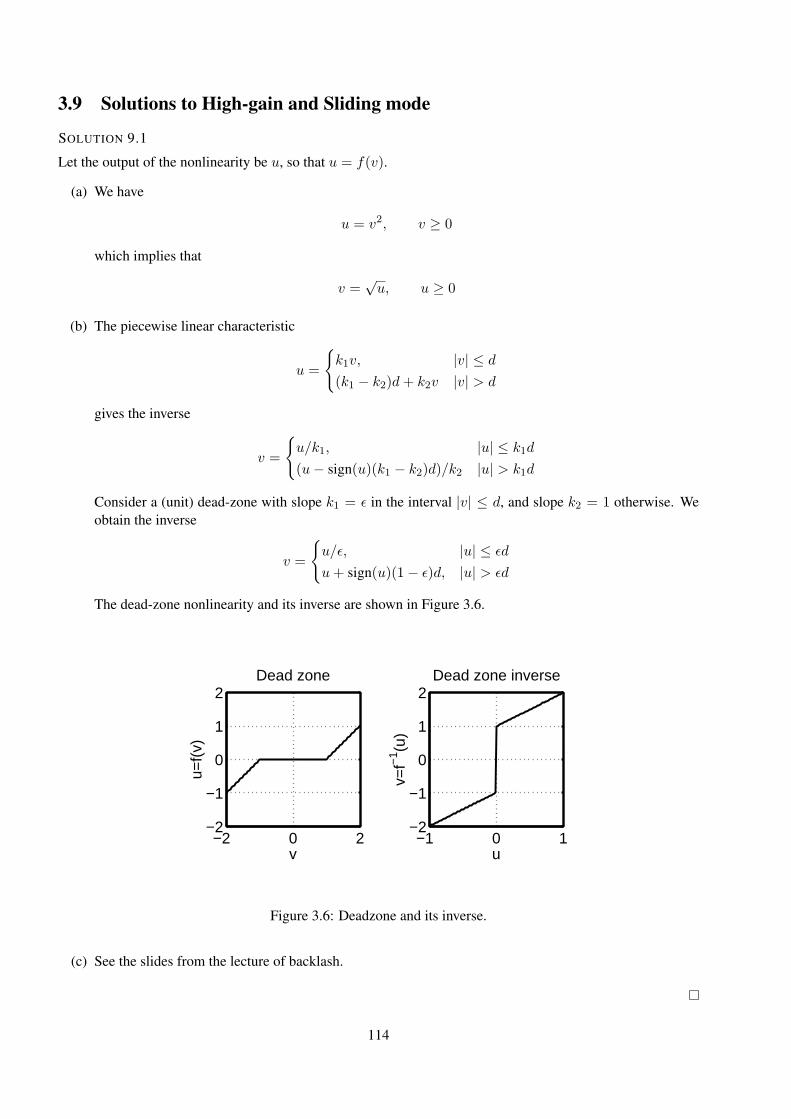
3.9 Solutions to High-gain and Sliding mode
SOLUTION 9.1
Let the output of the nonlinearity be u, so that u = f(v).
(a) We have
u = v2, v ≥ 0
which implies that
v =√u, u ≥ 0
(b) The piecewise linear characteristic
u =
k1v, |v| ≤ d
(k1 − k2)d+ k2v |v| > d
gives the inverse
v =
u/k1, |u| ≤ k1d
(u− sign(u)(k1 − k2)d)/k2 |u| > k1d
Consider a (unit) dead-zone with slope k1 = ǫ in the interval |v| ≤ d, and slope k2 = 1 otherwise. Weobtain the inverse
v =
u/ǫ, |u| ≤ ǫd
u+ sign(u)(1− ǫ)d, |u| > ǫd
The dead-zone nonlinearity and its inverse are shown in Figure 3.6.
−2 0 2−2
−1
0
1
2
v
u=f(
v)
Dead zone
−1 0 1−2
−1
0
1
2
u
v=f−
1 (u)
Dead zone inverse
Figure 3.6: Deadzone and its inverse.
(c) See the slides from the lecture of backlash.
114
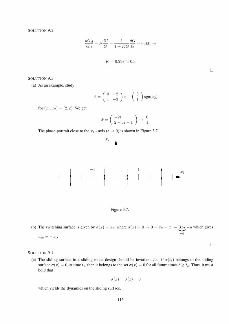
SOLUTION 9.2
dGcl
Gcl= S
dG
G=
1
1 +KG
dG
G= 0.001 ⇒
K = 0.298 ≈ 0.3
SOLUTION 9.3
(a) As an example, study
x =
(0 −21 −3
)x−
(01
)sgn(x2)
for (x1, x2) = (2, ε). We get
x =
(−2ε2− 3ε− 1
)→ 0
1
The phase-portrait close to the x1 - axis (ε→ 0) is shown in Figure 3.7.
x1
x2
1−1
Figure 3.7:
(b) The switching surface is given by σ(x) = x2, where σ(x) = 0 ⇒ 0 = x2 = x1 − 3x2︸︷︷︸=0
+u which gives
ueq = −x1.
SOLUTION 9.4
(a) The sliding surface in a sliding mode design should be invariant, i.e., if x(ts) belongs to the slidingsurface σ(x) = 0, at time ts, then it belongs to the set σ(x) = 0 for all future times t ≥ ts. Thus, it musthold that
σ(x) = σ(x) = 0
which yields the dynamics on the sliding surface.
115
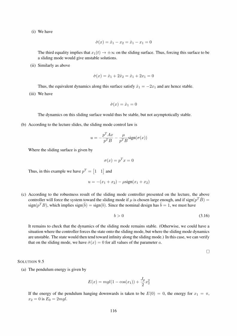
(i) We have
σ(x) = x1 − x2 = x1 − x1 = 0
The third equality implies that x1(t) → ±∞ on the sliding surface. Thus, forcing this surface to bea sliding mode would give unstable solutions.
(ii) Similarly as above
σ(x) = x1 + 2x2 = x1 + 2x1 = 0
Thus, the equivalent dynamics along this surface satisfy x1 = −2x1 and are hence stable.
(iii) We have
σ(x) = x1 = 0
The dynamics on this sliding surface would thus be stable, but not asymptotically stable.
(b) According to the lecture slides, the sliding mode control law is
u = −pTAx
pTB− µ
pTBsign(σ(x))
Where the sliding surface is given by
σ(x) = pTx = 0
Thus, in this example we have pT =[1 1
]and
u = −(x1 + x2)− µsign(x1 + x2)
(c) According to the robustness result of the sliding mode controller presented on the lecture, the abovecontroller will force the system toward the sliding mode if µ is chosen large enough, and if sign(pT B) =sign(pTB), which implies sign(b) = sign(b). Since the nominal design has b = 1, we must have
b > 0 (3.16)
It remains to check that the dynamics of the sliding mode remains stable. (Otherwise, we could have asituation where the controller forces the state onto the sliding mode, but where the sliding mode dynamicsare unstable. The state would then tend toward infinity along the sliding mode.) In this case, we can verifythat on the sliding mode, we have σ(x) = 0 for all values of the parameter a.
SOLUTION 9.5
(a) The pendulum energy is given by
E(x) = mgl(1− cos(x1)) +Jp2x22
If the energy of the pendulum hanging downwards is taken to be E(0) = 0, the energy for x1 = π,x2 = 0 is E0 = 2mgl.
116
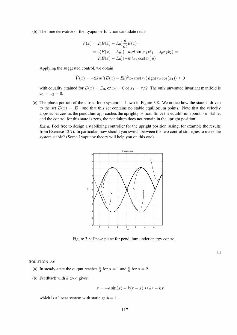
(b) The time derivative of the Lyapunov function candidate reads
V (x) = 2(E(x)− E0)d
dtE(x) =
= 2(E(x)− E0)(−mgl sin(x1)x1 + Jpx2x2) =
= 2(E(x)− E0)(−mlx2 cos(x1)u)
Applying the suggested control, we obtain
V (x) = −2kml(E(x)− E0)2x2 cos(x1)sign(x2 cos(x1)) ≤ 0
with equality attained for E(x) = E0, or x2 = 0 or x1 = π/2. The only unwanted invariant manifold isx1 = x2 = 0.
(c) The phase portrait of the closed loop system is shown in Figure 3.8. We notice how the state is drivento the set E(x) = E0, and that this set contains no stable equilibrium points. Note that the velocityapproaches zero as the pendulum approaches the upright position. Since the equilibrium point is unstable,and the control for this state is zero, the pendulum does not remain in the upright position.
Extra. Feel free to design a stabilizing controller for the upright position (using, for example the resultsfrom Exercise 12.7). In particular, how should you switch between the two control strategies to make thesystem stable? (Some Lyapunov theory will help you on this one)
−6 −4 −2 0 2 4 6−10
−8
−6
−4
−2
0
2
4
6
8
10
x1
x2
Phase plane
Figure 3.8: Phase plane for pendulum under energy control.
SOLUTION 9.6
(a) In steady-state the output reaches π2 for a = 1 and π
6 for a = 2.
(b) Feedback with k ≫ a gives
x = −a sin(x) + k(r − x) ≈ kr − kx
which is a linear system with static gain = 1.
117
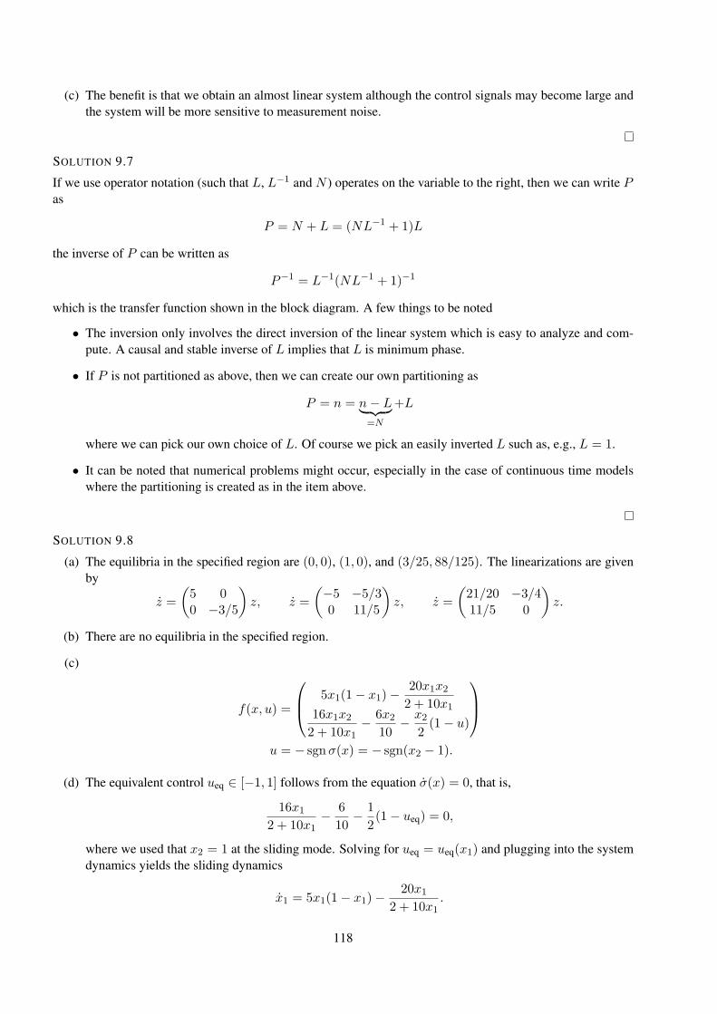
(c) The benefit is that we obtain an almost linear system although the control signals may become large andthe system will be more sensitive to measurement noise.
SOLUTION 9.7
If we use operator notation (such that L, L−1 and N ) operates on the variable to the right, then we can write Pas
P = N + L = (NL−1 + 1)L
the inverse of P can be written as
P−1 = L−1(NL−1 + 1)−1
which is the transfer function shown in the block diagram. A few things to be noted
• The inversion only involves the direct inversion of the linear system which is easy to analyze and com-pute. A causal and stable inverse of L implies that L is minimum phase.
• If P is not partitioned as above, then we can create our own partitioning as
P = n = n− L︸ ︷︷ ︸=N
+L
where we can pick our own choice of L. Of course we pick an easily inverted L such as, e.g., L = 1.
• It can be noted that numerical problems might occur, especially in the case of continuous time modelswhere the partitioning is created as in the item above.
SOLUTION 9.8
(a) The equilibria in the specified region are (0, 0), (1, 0), and (3/25, 88/125). The linearizations are givenby
z =
(5 00 −3/5
)z, z =
(−5 −5/30 11/5
)z, z =
(21/20 −3/411/5 0
)z.
(b) There are no equilibria in the specified region.
(c)
f(x, u) =
5x1(1− x1)−20x1x22 + 10x1
16x1x22 + 10x1
− 6x210
− x22(1− u)
u = − sgnσ(x) = − sgn(x2 − 1).
(d) The equivalent control ueq ∈ [−1, 1] follows from the equation σ(x) = 0, that is,
16x12 + 10x1
− 6
10− 1
2(1− ueq) = 0,
where we used that x2 = 1 at the sliding mode. Solving for ueq = ueq(x1) and plugging into the systemdynamics yields the sliding dynamics
x1 = 5x1(1− x1)−20x1
2 + 10x1.
118
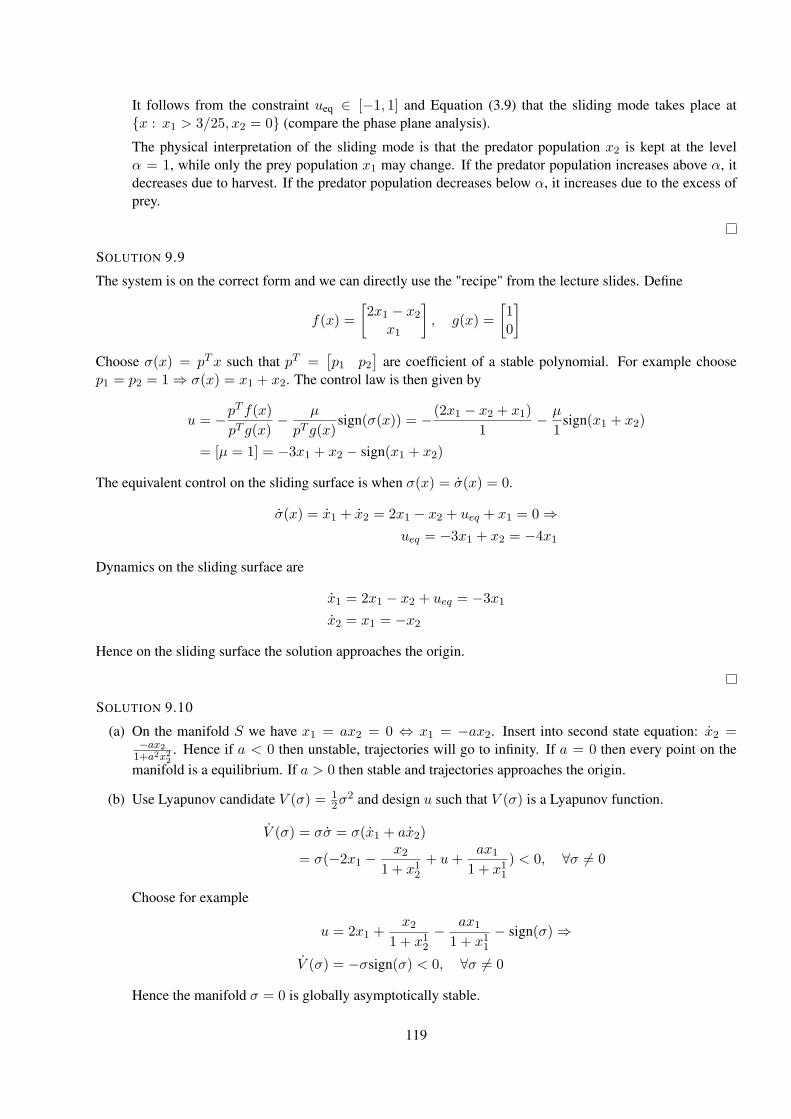
It follows from the constraint ueq ∈ [−1, 1] and Equation (3.9) that the sliding mode takes place atx : x1 > 3/25, x2 = 0 (compare the phase plane analysis).
The physical interpretation of the sliding mode is that the predator population x2 is kept at the levelα = 1, while only the prey population x1 may change. If the predator population increases above α, itdecreases due to harvest. If the predator population decreases below α, it increases due to the excess ofprey.
SOLUTION 9.9
The system is on the correct form and we can directly use the "recipe" from the lecture slides. Define
f(x) =
[2x1 − x2
x1
], g(x) =
[10
]
Choose σ(x) = pTx such that pT =[p1 p2
]are coefficient of a stable polynomial. For example choose
p1 = p2 = 1 ⇒ σ(x) = x1 + x2. The control law is then given by
u = −pT f(x)
pT g(x)− µ
pT g(x)sign(σ(x)) = −(2x1 − x2 + x1)
1− µ
1sign(x1 + x2)
= [µ = 1] = −3x1 + x2 − sign(x1 + x2)
The equivalent control on the sliding surface is when σ(x) = σ(x) = 0.
σ(x) = x1 + x2 = 2x1 − x2 + ueq + x1 = 0 ⇒ueq = −3x1 + x2 = −4x1
Dynamics on the sliding surface are
x1 = 2x1 − x2 + ueq = −3x1
x2 = x1 = −x2
Hence on the sliding surface the solution approaches the origin.
SOLUTION 9.10
(a) On the manifold S we have x1 = ax2 = 0 ⇔ x1 = −ax2. Insert into second state equation: x2 =−ax2
1+a2x2
2
. Hence if a < 0 then unstable, trajectories will go to infinity. If a = 0 then every point on the
manifold is a equilibrium. If a > 0 then stable and trajectories approaches the origin.
(b) Use Lyapunov candidate V (σ) = 12σ
2 and design u such that V (σ) is a Lyapunov function.
V (σ) = σσ = σ(x1 + ax2)
= σ(−2x1 −x2
1 + x12+ u+
ax11 + x11
) < 0, ∀σ 6= 0
Choose for example
u = 2x1 +x2
1 + x12− ax1
1 + x11− sign(σ) ⇒
V (σ) = −σsign(σ) < 0, ∀σ 6= 0
Hence the manifold σ = 0 is globally asymptotically stable.
119
(c) On the sliding manifold we have
σ(x) = σ(x) = 0 ⇒σ(x) = x1 + ax2 = −2x1 −
x21 + x12
+ ueq +ax1
1 + x11= 0 ⇒
ueq = 2x1 +x2
1 + x12− ax1
1 + x11
3.10 Solutions to Computer Exercises: Sliding Mode, IMC and Gain schedul-
ing
SOLUTION 10.1
(a) Straightforward manipulations give
G(s) =K
sT + 1e−sL =
1
sVm/q(t) + 1e−sVd/q(t)
(b) The step response gives parameters a = 0.9, L = 1. Using the results from (a) and a = KL/T weobtain
a = Vd/Vm
L = Vd/q(t)
Since the experiment was performed for q(t) = 1, we see that L = 1/q(t). Now, a gain scheduled PIcontroller can be constructed using Ziegler-Nichols recommendations as
Kp = 0.9/a = 1
Ti = 3L = 3/q(t)
(c) One way of implementing the controlled system is shown in Figure 3.9.
120
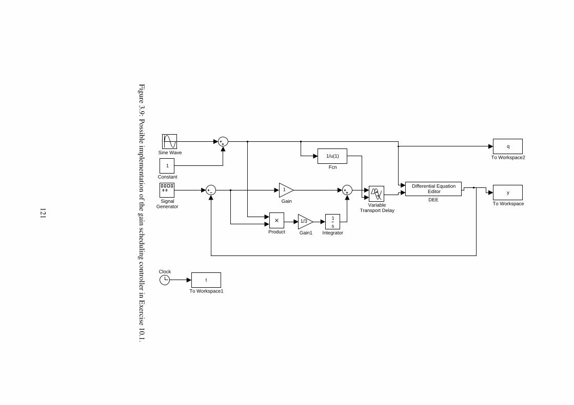
VariableTransport Delay
q
To Workspace2
t
To Workspace1
y
To Workspace
Sine Wave
SignalGenerator
Products
1
Integrator
1/3
Gain1
1
Gain
1/u(1)
Fcn
Differential Equation Editor
DEE
1
Constant
Clock
Figure3.9:
Possibleim
plementation
ofthe
gainscheduling
controllerin
Exercise
10.1.
121
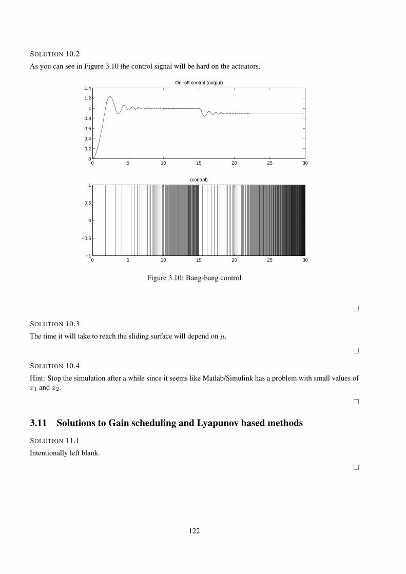
SOLUTION 10.2
As you can see in Figure 3.10 the control signal will be hard on the actuators.
0 5 10 15 20 25 300
0.2
0.4
0.6
0.8
1
1.2
1.4On−off control (output)
0 5 10 15 20 25 30−1
−0.5
0
0.5
1(control)
Figure 3.10: Bang-bang control
SOLUTION 10.3
The time it will take to reach the sliding surface will depend on µ.
SOLUTION 10.4
Hint: Stop the simulation after a while since it seems like Matlab/Simulink has a problem with small values ofx1 and x2.
3.11 Solutions to Gain scheduling and Lyapunov based methods
SOLUTION 11.1
Intentionally left blank.
122
SOLUTION 11.2
(a) With u = −z the x(t) is given by
x(t) =2x0
(2− x0z20)et + x0z20e−t
which will have finite escape time if x0z20 > 2.
(b) With K = (−1 − 1) we get u = −z1 − z2 − x3
SOLUTION 11.3
For the nominal system we use ψ(x) = −(x31+x1+2x32+x2) and with ρ(x) =√x21(1 + x1)2 + x22(1 + x2)2
and k = 0.5 we can use
u = ψ(x)− ρ(x)
1− ksqn
(dV
dxg(x)
)
= −x31 − x1 − 2x32 − x2 − 2ρ(x) sqn (x1 + x2)
SOLUTION 11.4
Left blank
SOLUTION 11.5
Left blank
SOLUTION 11.6
u = (−2x1 − 1)(x21 − x31 + x2)− x1 − (x2 + x21 + x1) (3.17)
SOLUTION 11.7
Left blank
SOLUTION 11.8
Left blank
SOLUTION 11.9
u = −2x21x2 − x21 − (x2 + x21)− x1
123
SOLUTION 11.12
(a) Plugging in the transformation and the control law gives
z =
(0 1−1 −2
)z
Since both eigenvalues of this matrix are −1, the system is asymptotically stable.
(b) Let
k(x) = u(z(x)) = −x1 − 2x2 − 2f(x1)− [x2 + f(x1)]f′(x1).
From the linear system in (a), we have the Lyapunov function V (z) = zTPz, where P = P T > 0 is thesolution to the Lyapunov equation PA+ATP = −Q. Choosing Q = 2I (the identity matrix) gives
P =
(3 11 1
)
Hence,
V (x) =
(z1z2
)T
P
(z1z2
)=
(x1
x2 + f(x1)
)T (3 11 1
)(x1
x2 + f(x1)
),
which is easily checked to fulfill the conditions for the Lyapunov theorem for global stability (includingV (x) → ∞ as ‖x‖ → ∞).
SOLUTION 11.13
(a) x = (r, r, θ, θ)T gives
x =
x1x2x3x4
=
x2−g sinx3 − βx2 + x1x
24
x4−2x1x2x4 − gx1 cosx3 + u
x21 + 1
= f(x, u)
(b) f(x0, u0) = 0 gives x0 = (x10, 0, kπ, 0)T with x10 and u0 being the solutions to the equation gx10 cos kπ =
u0 and k being an integer.
(c) Take x0 = (0, 0, 0, 0)T and u0 = 0. Then,
∂f
∂x(x0, u0) =
0 1 0 00 −β −g 00 0 0 1−g 0 0 0
,
∂f
∂u(x0, u0) =
0001
.
(d) Denote the linearization in (c) by
δx = Aδx+Bδu.
Choosing L = (ℓ1, ℓ2, ℓ3, ℓ4) such that the eigenvalues ofA−BL are in the left half-plane gives a controllaw u = −Lx, which is stabilizing also for x = f(x, u).
124
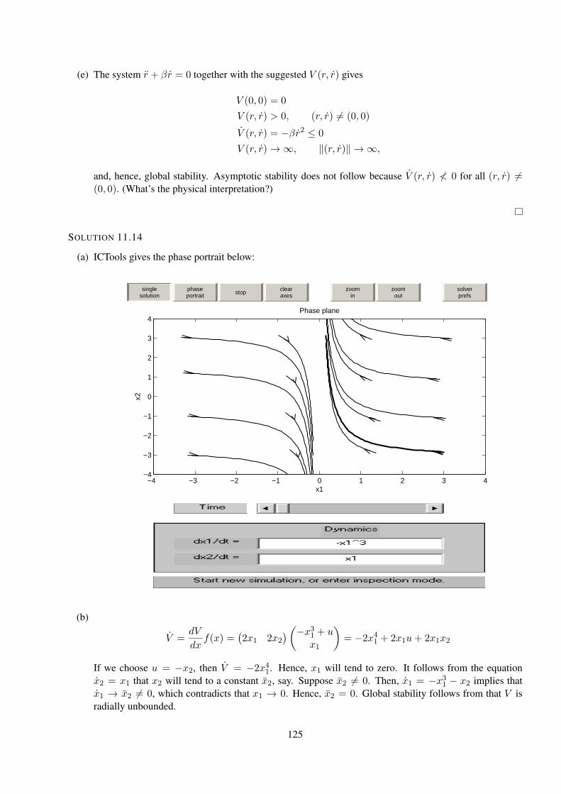
(e) The system r + βr = 0 together with the suggested V (r, r) gives
V (0, 0) = 0
V (r, r) > 0, (r, r) 6= (0, 0)
V (r, r) = −βr2 ≤ 0
V (r, r) → ∞, ‖(r, r)‖ → ∞,
and, hence, global stability. Asymptotic stability does not follow because V (r, r) 6< 0 for all (r, r) 6=(0, 0). (What’s the physical interpretation?)
SOLUTION 11.14
(a) ICTools gives the phase portrait below:
singlesolution
phaseportrait stop clear
axeszoom
inzoomout
solverprefs
−4 −3 −2 −1 0 1 2 3 4−4
−3
−2
−1
0
1
2
3
4
x1
x2
Phase plane
(b)
V =dV
dxf(x) =
(2x1 2x2
)(−x31 + ux1
)= −2x41 + 2x1u+ 2x1x2
If we choose u = −x2, then V = −2x41. Hence, x1 will tend to zero. It follows from the equationx2 = x1 that x2 will tend to a constant x2, say. Suppose x2 6= 0. Then, x1 = −x31 − x2 implies thatx1 → x2 6= 0, which contradicts that x1 → 0. Hence, x2 = 0. Global stability follows from that V isradially unbounded.
125
(c) Choosing u = x31 + v gives the system
x1 = v
x2 = x1,
which is globally stabilized, for example, by v = −2x1 − x2. Hence,
u = x31 − 2x1 − x2
is a possible control law.
3.12 Solutions to Feedback linearization
SOLUTION 12.1
The control is given by
u = φ(x1) + ψ(x2)− a1x1 − a2x2 + r.
SOLUTION 12.2
The system is defined by
(∗)
x1 = x21 + x2x2 = uy = x1
Change of variables z1 = yz2 = y
givingz1 = y = z2
z2 = y =d
dt(x1)
=d
dt
(x21 + x2
)
= 2x1x1 + x2 = [from (∗)]= 2x1
(x21 + x2
)+ u
=
(∗) ⇒ x2 = x1 − x21x1 = y = z1x1 = y = z2
= 2z1(z21 + z2 − z21
)+ u
= 2z1z2 + u = α(z) + β(z)u
An exact linearization is then
u =−α(z) + u
β(z)= −2z1z2 + u.
126
SOLUTION 12.3
(a) With y = x2.
y = x2 =√1 + x1 −
√1 + x2
y = x2 =d
dt
(√1 + x1 −
√1 + x2
)=
=1
2√1 + x1
x1 −1
2√1 + x2
x2 = · · · =
=1
2
(1√
1 + x1−
√1 + x1√1 + x2
)+
u
2√1 + x1
It follows that the relative degree is 2.
(b,c) Select the states z1 = y, z2 = y ⇒
z1 = z2
z2 = /as above/ =1
2
(1√
1 + x1−
√1 + x1√1 + x2
)+
u
2√1 + x1
=
=
∣∣∣∣z1 = y = x2z2 = y = x2 =
√1 + x1 −
√1 + x2
⇒x2 = z1√1 + x1 = z2 +
√1 + z1
∣∣∣∣ =
=1
2
(1
z2 +√1 + z1
− z2 +√1 + z1√
1 + z1
)+
1
2
1
z2 +√1 + z1
u =
= α(z) + β(z)u
Now choose u = 1β(z) (u− α(z)) to obtain a feedback law based achieving an exact linearization.
SOLUTION 12.4
G :
x1 = −x1 + 7x2x2 = −x2 + cosx1 + ω
Desired: u exactly linearizing the system.Obtained by: u = r − cosx1
SOLUTION 12.5
u = −y4 + y2 + r = −x41 + x21 + r
SOLUTION 12.7
(a) We notice that all state equation but the last one are linear. The last state equation reads
xn = f(x) + g(x)u
If we assume that g(x) 6= 0 for all x, we can apply the control
u = h(x, v) =1
g(x)(−f(x) + Lx+ v)
127
renders the last state equation linear
xn = Lx+ v
The response from v to x is linear, and the closed loop dynamics is given by
x =
0 1 0 0 00 0 1 0 . . .
0 0 0. . . 0
l1 l2 l3 . . . ln
x+
00...1
v
(You may recognize this as the controller form from the basic control course). For the control to be welldefined, we must require that g(x) 6= 0 for all x.
(b) The above procedure suggest the control
u =1
b cos(x1)(−a sin(x1) + l1x1 + l2x2 + v)
which results in the closed loop system
x =
[0 1l1 l2
]x+
[01
]v
The system matrix has a double eigenvalue in s = −1 if we let
l1 = −1, l2 = −2
The control law is well defined for x1 6= π/2. This corresponds to the pendulum being horizontal. Forx1 = π/2, u has no influence on the system. Notice how the control “blows up” nearby this singularity.Extra. You may want to verify by simulations the behavior of the modified control
u = sat(h(x, v))
for different values of the saturation level.
(c) The above procedure suggest the control
u = −x2 − x+ v
Letting v = 0, we apply the control to the perturbed system
x = (1 + ǫ)x2 − x2 − x = ǫx2 − x
and note that for x > 1/ǫ, we have x > 0, which implies that the trajectories tend to infinity. Thus,global cancellation is non-robust in the sense that it may require a very precise mathematical model.
128
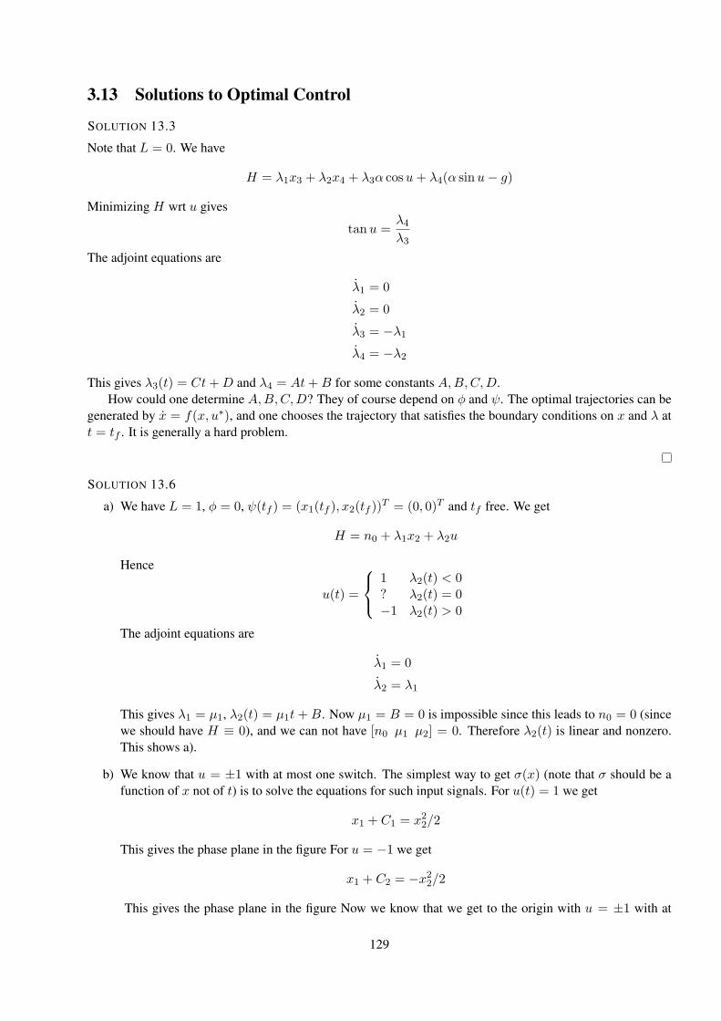
3.13 Solutions to Optimal Control
SOLUTION 13.3
Note that L = 0. We have
H = λ1x3 + λ2x4 + λ3α cosu+ λ4(α sinu− g)
Minimizing H wrt u gives
tanu =λ4λ3
The adjoint equations are
λ1 = 0
λ2 = 0
λ3 = −λ1λ4 = −λ2
This gives λ3(t) = Ct+D and λ4 = At+B for some constants A,B,C,D.How could one determine A,B,C,D? They of course depend on φ and ψ. The optimal trajectories can be
generated by x = f(x, u∗), and one chooses the trajectory that satisfies the boundary conditions on x and λ att = tf . It is generally a hard problem.
SOLUTION 13.6
a) We have L = 1, φ = 0, ψ(tf ) = (x1(tf ), x2(tf ))T = (0, 0)T and tf free. We get
H = n0 + λ1x2 + λ2u
Hence
u(t) =
1 λ2(t) < 0? λ2(t) = 0−1 λ2(t) > 0
The adjoint equations are
λ1 = 0
λ2 = λ1
This gives λ1 = µ1, λ2(t) = µ1t+B. Now µ1 = B = 0 is impossible since this leads to n0 = 0 (sincewe should have H ≡ 0), and we can not have [n0 µ1 µ2] = 0. Therefore λ2(t) is linear and nonzero.This shows a).
b) We know that u = ±1 with at most one switch. The simplest way to get σ(x) (note that σ should be afunction of x not of t) is to solve the equations for such input signals. For u(t) = 1 we get
x1 + C1 = x22/2
This gives the phase plane in the figure For u = −1 we get
x1 + C2 = −x22/2
This gives the phase plane in the figure Now we know that we get to the origin with u = ±1 with at
129
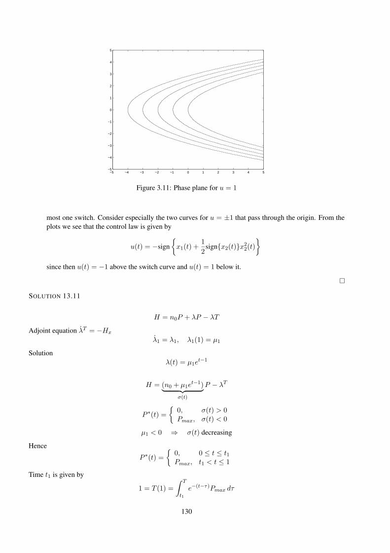
−5 −4 −3 −2 −1 0 1 2 3 4 5−5
−4
−3
−2
−1
0
1
2
3
4
5
Figure 3.11: Phase plane for u = 1
most one switch. Consider especially the two curves for u = ±1 that pass through the origin. From theplots we see that the control law is given by
u(t) = −signx1(t) +
1
2signx2(t)x22(t)
since then u(t) = −1 above the switch curve and u(t) = 1 below it.
SOLUTION 13.11
H = n0P + λP − λT
Adjoint equation λT = −Hx
λ1 = λ1, λ1(1) = µ1
Solutionλ(t) = µ1e
t−1
H = (n0 + µ1et−1)︸ ︷︷ ︸
σ(t)
P − λT
P ∗(t) =
0, σ(t) > 0Pmax, σ(t) < 0
µ1 < 0 ⇒ σ(t) decreasing
Hence
P ∗(t) =
0, 0 ≤ t ≤ t1Pmax, t1 < t ≤ 1
Time t1 is given by
1 = T (1) =
∫ T
t1
e−(t−τ)Pmax dτ
130
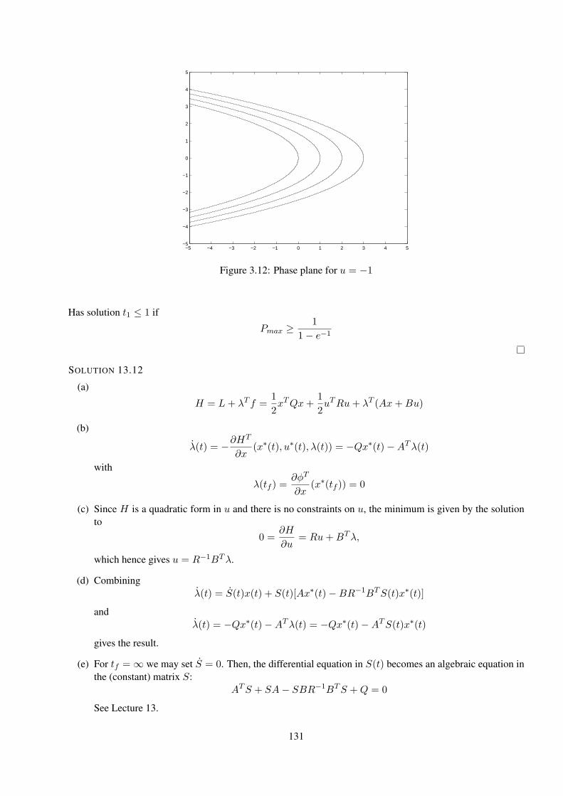
−5 −4 −3 −2 −1 0 1 2 3 4 5−5
−4
−3
−2
−1
0
1
2
3
4
5
Figure 3.12: Phase plane for u = −1
Has solution t1 ≤ 1 if
Pmax ≥ 1
1− e−1
SOLUTION 13.12
(a)
H = L+ λT f =1
2xTQx+
1
2uTRu+ λT (Ax+Bu)
(b)
λ(t) = −∂HT
∂x(x∗(t), u∗(t), λ(t)) = −Qx∗(t)−ATλ(t)
with
λ(tf ) =∂φT
∂x(x∗(tf )) = 0
(c) Since H is a quadratic form in u and there is no constraints on u, the minimum is given by the solutionto
0 =∂H
∂u= Ru+BTλ,
which hence gives u = R−1BTλ.
(d) Combiningλ(t) = S(t)x(t) + S(t)[Ax∗(t)−BR−1BTS(t)x∗(t)]
andλ(t) = −Qx∗(t)−ATλ(t) = −Qx∗(t)−ATS(t)x∗(t)
gives the result.
(e) For tf = ∞ we may set S = 0. Then, the differential equation in S(t) becomes an algebraic equation inthe (constant) matrix S:
ATS + SA− SBR−1BTS +Q = 0
See Lecture 13.
131
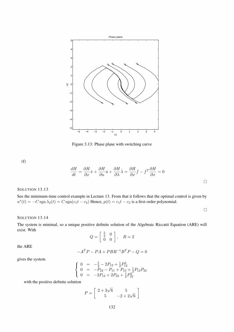
−5 −4 −3 −2 −1 0 1 2 3 4−5
−4
−3
−2
−1
0
1
2
3
4
5
x1
x2
Phase plane
Figure 3.13: Phase plane with switching curve
(f)
dH
dt=∂H
∂xx+
∂H
∂uu+
∂H
∂λλ =
∂H
∂xf − fT
∂H
∂x= 0
SOLUTION 13.13
See the minimum-time control example in Lecture 13. From that it follows that the optimal control is given byu∗(t) = −C sgnλ2(t) = C sgn(c1t− c2) Hence, p(t) = c1t− c2 is a first-order polynomial.
SOLUTION 13.14
The system is minimal, so a unique positive definite solution of the Algebraic Riccatti Equation (ARE) willexist. With
Q =
[52 00 0
], R = 2
the ARE−ATP − PA+ PBR−1BTP −Q = 0
gives the system
0 = −52 − 2P12 +
12P
212
0 = −P22 − P11 + P12 +12P12P22
0 = −2P12 + 2P22 +12P
222
with the positive definite solution
P =
[2 + 3
√6 5
5 −2 + 2√6
]
132
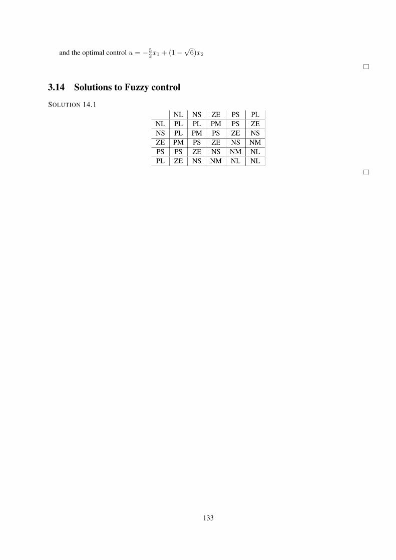
and the optimal control u = −52x1 + (1−
√6)x2
3.14 Solutions to Fuzzy control
SOLUTION 14.1NL NS ZE PS PL
NL PL PL PM PS ZENS PL PM PS ZE NSZE PM PS ZE NS NMPS PS ZE NS NM NLPL ZE NS NM NL NL
133


![HOMEWORK EXERCISES Very Preliminaryfaculty.bard.edu/bloch/math104_exercises.pdf · Homework Exercise NAME Section 1.2: Homework Exercise 1 [VotingMethods] SupposethatanelectionhascandidatesA,B,C](https://img.pdfslide.us/doc/110x75/5f0951277e708231d4264091/homework-exercises-very-homework-exercise-name-section-12-homework-exercise-1.jpg)