El Nino Southern Oscillation (ENSO)☆

KE Trenberth, National Center for Atmospheric Research, Boulder, CO, USA

ã 2013 Elsevier Inc. All rights reserved.

Introduction 1ENSO Events 1The Tropical Pacific Ocean – Atmosphere System 2Mechanisms of ENSO 7Interannual Variations in Climate 8Impacts 11ENSO and Seasonal Predictions 11

Introduction

A major El Nino began in April of 1997 and continued until May 1998. It was labeled by some as the ‘El Nino of the century’ as it

was certainly the biggest on record by several measures. It brought with it many weather extremes and unusual weather patterns

around the world. Moreover, the event was predicted by climate scientists and received unprecedented news coverage, so that the

term ‘El Nino’ became part of the popular vernacular. Many things were blamed on El Nino, and some of them indeed were

influenced by El Nino, although in some instances, the connection was, at best, tenuous. Although El Nino was relatively new to the

public, it had been known to scientists, at least in some respects, for decades and even centuries.

El Nino refers to the exceptionally warm sea temperatures in the tropical Pacific, but it is linked to major changes in the

atmosphere through the phenomenon known as the Southern Oscillation (SO), in particular, so that the whole phenomenon is

called El Nino–Southern Oscillation (ENSO) by scientists. This article outlines the current understanding of ENSO and the physical

connections between the tropical Pacific and the rest of the world.

ENSO Events

El Ninos are not uncommon. Every three to seven years or so, a pronounced warming occurs of the surface waters of the tropical

Pacific Ocean. The warmings take place from the International Dateline to the west coast of South America and result in changes in

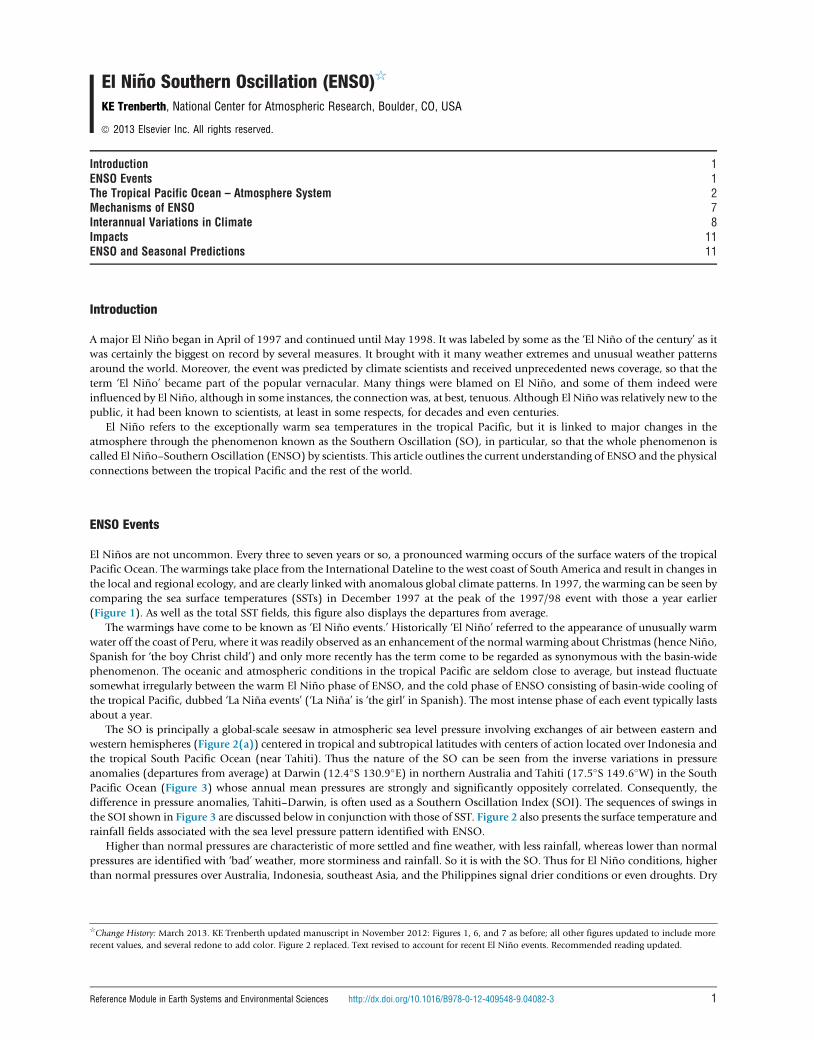
the local and regional ecology, and are clearly linked with anomalous global climate patterns. In 1997, the warming can be seen by

comparing the sea surface temperatures (SSTs) in December 1997 at the peak of the 1997/98 event with those a year earlier

(Figure 1). As well as the total SST fields, this figure also displays the departures from average.

The warmings have come to be known as ‘El Nino events.’ Historically ‘El Nino’ referred to the appearance of unusually warm

water off the coast of Peru, where it was readily observed as an enhancement of the normal warming about Christmas (hence Nino,

Spanish for ‘the boy Christ child’) and only more recently has the term come to be regarded as synonymous with the basin-wide

phenomenon. The oceanic and atmospheric conditions in the tropical Pacific are seldom close to average, but instead fluctuate

somewhat irregularly between the warm El Nino phase of ENSO, and the cold phase of ENSO consisting of basin-wide cooling of

the tropical Pacific, dubbed ‘La Nina events’ (‘La Nina’ is ‘the girl’ in Spanish). The most intense phase of each event typically lasts

about a year.

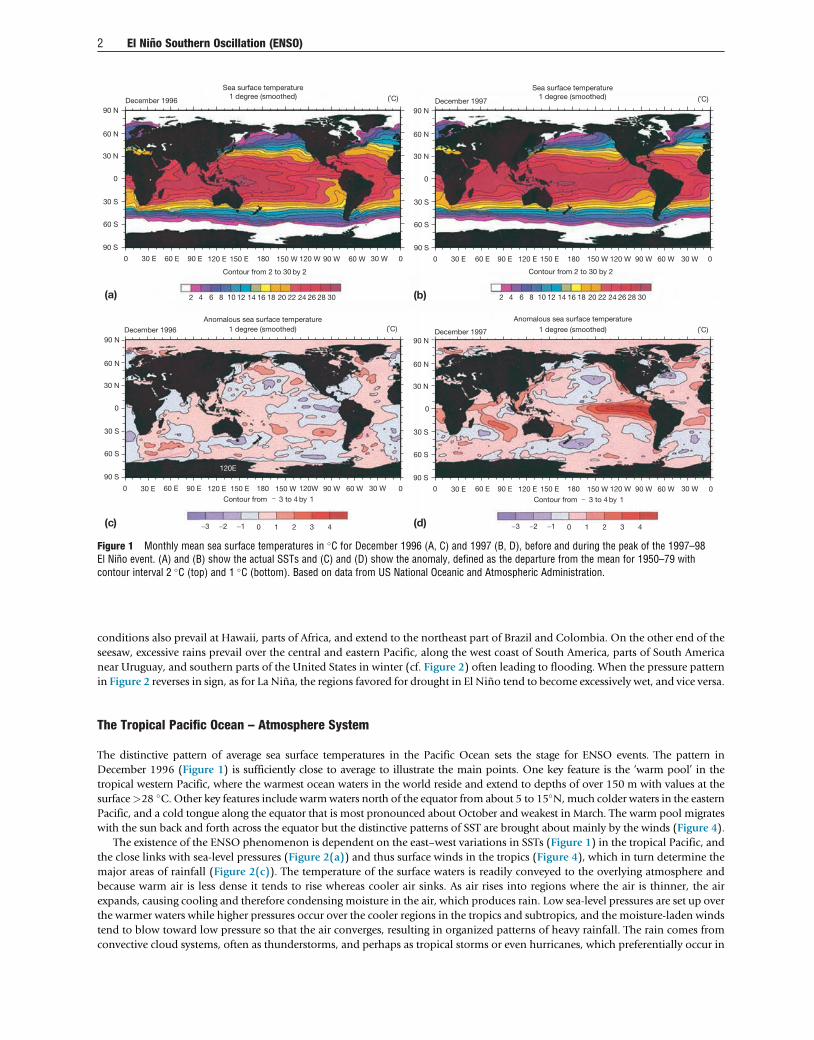
The SO is principally a global-scale seesaw in atmospheric sea level pressure involving exchanges of air between eastern and

western hemispheres (Figure 2(a)) centered in tropical and subtropical latitudes with centers of action located over Indonesia and

the tropical South Pacific Ocean (near Tahiti). Thus the nature of the SO can be seen from the inverse variations in pressure

anomalies (departures from average) at Darwin (12.4�S 130.9�E) in northern Australia and Tahiti (17.5�S 149.6�W) in the South

Pacific Ocean (Figure 3) whose annual mean pressures are strongly and significantly oppositely correlated. Consequently, the

difference in pressure anomalies, Tahiti–Darwin, is often used as a Southern Oscillation Index (SOI). The sequences of swings in

the SOI shown in Figure 3 are discussed below in conjunction with those of SST. Figure 2 also presents the surface temperature and

rainfall fields associated with the sea level pressure pattern identified with ENSO.

Higher than normal pressures are characteristic of more settled and fine weather, with less rainfall, whereas lower than normal

pressures are identified with ‘bad’ weather, more storminess and rainfall. So it is with the SO. Thus for El Nino conditions, higher

than normal pressures over Australia, Indonesia, southeast Asia, and the Philippines signal drier conditions or even droughts. Dry

☆Change History: March 2013. KE Trenberth updated manuscript in November 2012: Figures 1, 6, and 7 as before; all other figures updated to include more

recent values, and several redone to add color. Figure 2 replaced. Text revised to account for recent El Nino events. Recommended reading updated.

Reference Module in Earth Systems and Environmental Sciences http://dx.doi.org/10.1016/B978-0-12-409548-9.04082-3 1

0 30 E 60 E 90 E 90 W 60 W 30 W 0120 E 120W150 E 150 W180

120E90 S

(c)

60 S

30 S

30 N

60 N

90 N

0

−3 −2 −1 0 1 2 3 4 −3 −2 −1 0 1 2 3 4

Contour from _ 3 to 4 by 1

December 1996Anomalous sea surface temperature

1 degree (smoothed) (˚C)

0 30 E 60 E 90 E 90 W 60 W 30 W 0120 E 120 W150 E 150 W180

90 S

(a)

60 S

30 S

30 N

60 N

90 N

0

Contour from 2 to 30 by 2

2 4 6 8 10 12 14 1816 20 22 24 26 28 30

December 1996

Sea surface temperature1 degree (smoothed) (˚C)

0 30 E 60 E 90 E 90 W 60 W 30 W 0120 E 120 W150 E 150 W180

90 S

60 S

30 S

30 N

60 N

90 N

0

Contour from 2 to 30 by 2

December 1997

Sea surface temperature1 degree (smoothed) (˚C)

0 30 E 60 E 90 E 90 W 60 W 30 W 0120 E 120 W150 E 150 W180

90 S

60 S

30 S

30 N

60 N

90 N

0

Contour from _ 3 to 4 by 1

2(b)

(d)

4 6 8 10 12 14 1816 20 22 24 26 28 30

December 1997

Anomalous sea surface temperature1 degree (smoothed) (˚C)

Figure 1 Monthly mean sea surface temperatures in �C for December 1996 (A, C) and 1997 (B, D), before and during the peak of the 1997–98El Nino event. (A) and (B) show the actual SSTs and (C) and (D) show the anomaly, defined as the departure from the mean for 1950–79 withcontour interval 2 �C (top) and 1 �C (bottom). Based on data from US National Oceanic and Atmospheric Administration.

2 El Nino Southern Oscillation (ENSO)

conditions also prevail at Hawaii, parts of Africa, and extend to the northeast part of Brazil and Colombia. On the other end of the

seesaw, excessive rains prevail over the central and eastern Pacific, along the west coast of South America, parts of South America

near Uruguay, and southern parts of the United States in winter (cf. Figure 2) often leading to flooding. When the pressure pattern

in Figure 2 reverses in sign, as for La Nina, the regions favored for drought in El Nino tend to become excessively wet, and vice versa.

The Tropical Pacific Ocean – Atmosphere System

The distinctive pattern of average sea surface temperatures in the Pacific Ocean sets the stage for ENSO events. The pattern in

December 1996 (Figure 1) is sufficiently close to average to illustrate the main points. One key feature is the ‘warm pool’ in the

tropical western Pacific, where the warmest ocean waters in the world reside and extend to depths of over 150 m with values at the

surface>28 �C. Other key features include warmwaters north of the equator from about 5 to 15�N,much colder waters in the eastern

Pacific, and a cold tongue along the equator that is most pronounced about October and weakest in March. The warm pool migrates

with the sun back and forth across the equator but the distinctive patterns of SST are brought about mainly by the winds (Figure 4).

The existence of the ENSO phenomenon is dependent on the east–west variations in SSTs (Figure 1) in the tropical Pacific, and

the close links with sea-level pressures (Figure 2(a)) and thus surface winds in the tropics (Figure 4), which in turn determine the

major areas of rainfall (Figure 2(c)). The temperature of the surface waters is readily conveyed to the overlying atmosphere and

because warm air is less dense it tends to rise whereas cooler air sinks. As air rises into regions where the air is thinner, the air

expands, causing cooling and therefore condensing moisture in the air, which produces rain. Low sea-level pressures are set up over

the warmer waters while higher pressures occur over the cooler regions in the tropics and subtropics, and the moisture-laden winds

tend to blow toward low pressure so that the air converges, resulting in organized patterns of heavy rainfall. The rain comes from

convective cloud systems, often as thunderstorms, and perhaps as tropical storms or even hurricanes, which preferentially occur in

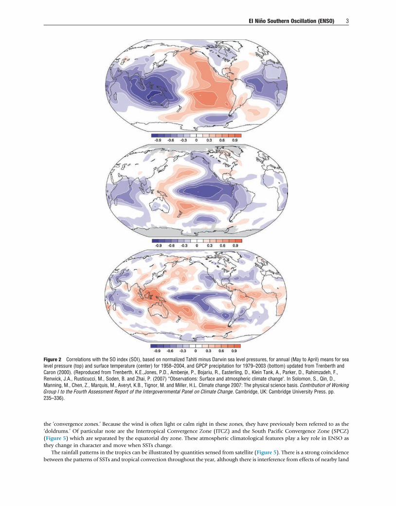
Figure 2 Correlations with the SO index (SOI), based on normalized Tahiti minus Darwin sea level pressures, for annual (May to April) means for sealevel pressure (top) and surface temperature (center) for 1958–2004, and GPCP precipitation for 1979–2003 (bottom) updated from Trenberth andCaron (2000). (Reproduced from Trenberth, K.E.,Jones, P.D., Ambenje, P., Bojariu, R., Easterling, D., Klein Tank, A., Parker, D., Rahimzadeh, F.,Renwick, J.A., Rusticucci, M., Soden, B. and Zhai, P. (2007) “Observations: Surface and atmospheric climate change". In Solomon, S., Qin, D.,Manning, M., Chen, Z., Marquis, M., Averyt, K.B., Tignor, M. and Miller, H.L. Climate change 2007: The physical science basis. Contribution of WorkingGroup I to the Fourth Assessment Report of the Intergovernmental Panel on Climate Change. Cambridge, UK: Cambridge University Press. pp.235–336).

El Nino Southern Oscillation (ENSO) 3

the ‘convergence zones.’ Because the wind is often light or calm right in these zones, they have previously been referred to as the

‘doldrums.’ Of particular note are the Intertropical Convergence Zone (ITCZ) and the South Pacific Convergence Zone (SPCZ)

(Figure 5) which are separated by the equatorial dry zone. These atmospheric climatological features play a key role in ENSO as

they change in character and move when SSTs change.

The rainfall patterns in the tropics can be illustrated by quantities sensed from satellite (Figure 5). There is a strong coincidence

between the patterns of SSTs and tropical convection throughout the year, although there is interference from effects of nearby land

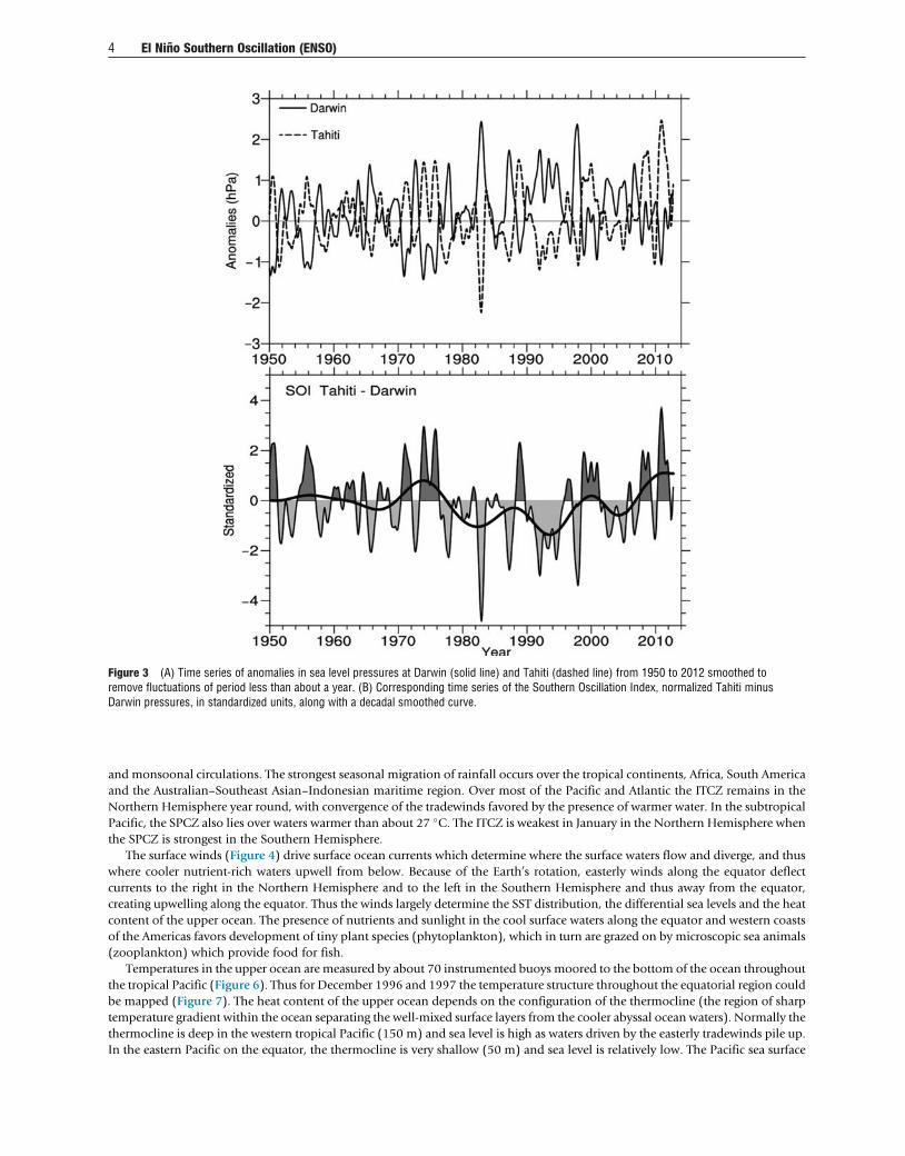
Figure 3 (A) Time series of anomalies in sea level pressures at Darwin (solid line) and Tahiti (dashed line) from 1950 to 2012 smoothed toremove fluctuations of period less than about a year. (B) Corresponding time series of the Southern Oscillation Index, normalized Tahiti minusDarwin pressures, in standardized units, along with a decadal smoothed curve.

4 El Nino Southern Oscillation (ENSO)

and monsoonal circulations. The strongest seasonal migration of rainfall occurs over the tropical continents, Africa, South America

and the Australian–Southeast Asian–Indonesian maritime region. Over most of the Pacific and Atlantic the ITCZ remains in the

Northern Hemisphere year round, with convergence of the tradewinds favored by the presence of warmer water. In the subtropical

Pacific, the SPCZ also lies over waters warmer than about 27 �C. The ITCZ is weakest in January in the Northern Hemisphere when

the SPCZ is strongest in the Southern Hemisphere.

The surface winds (Figure 4) drive surface ocean currents which determine where the surface waters flow and diverge, and thus

where cooler nutrient-rich waters upwell from below. Because of the Earth’s rotation, easterly winds along the equator deflect

currents to the right in the Northern Hemisphere and to the left in the Southern Hemisphere and thus away from the equator,

creating upwelling along the equator. Thus the winds largely determine the SST distribution, the differential sea levels and the heat

content of the upper ocean. The presence of nutrients and sunlight in the cool surface waters along the equator and western coasts

of the Americas favors development of tiny plant species (phytoplankton), which in turn are grazed on by microscopic sea animals

(zooplankton) which provide food for fish.

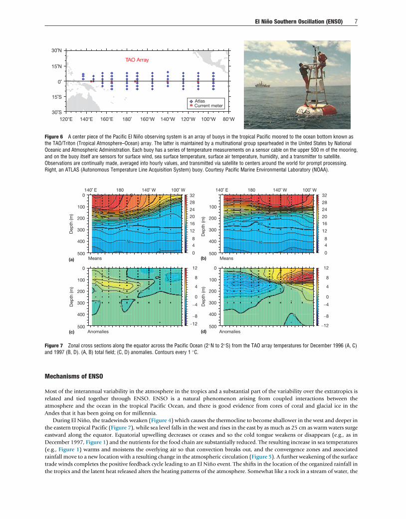
Temperatures in the upper ocean are measured by about 70 instrumented buoys moored to the bottom of the ocean throughout

the tropical Pacific (Figure 6). Thus for December 1996 and 1997 the temperature structure throughout the equatorial region could

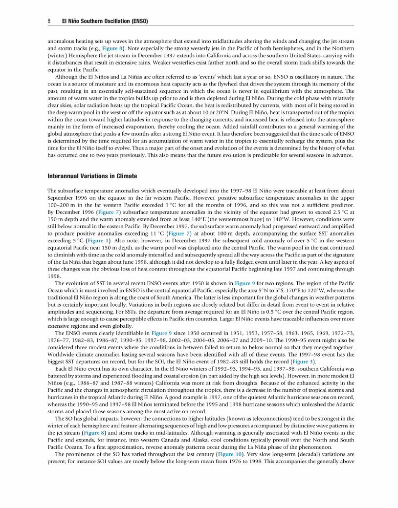
be mapped (Figure 7). The heat content of the upper ocean depends on the configuration of the thermocline (the region of sharp

temperature gradient within the ocean separating the well-mixed surface layers from the cooler abyssal ocean waters). Normally the

thermocline is deep in the western tropical Pacific (150 m) and sea level is high as waters driven by the easterly tradewinds pile up.

In the eastern Pacific on the equator, the thermocline is very shallow (50 m) and sea level is relatively low. The Pacific sea surface

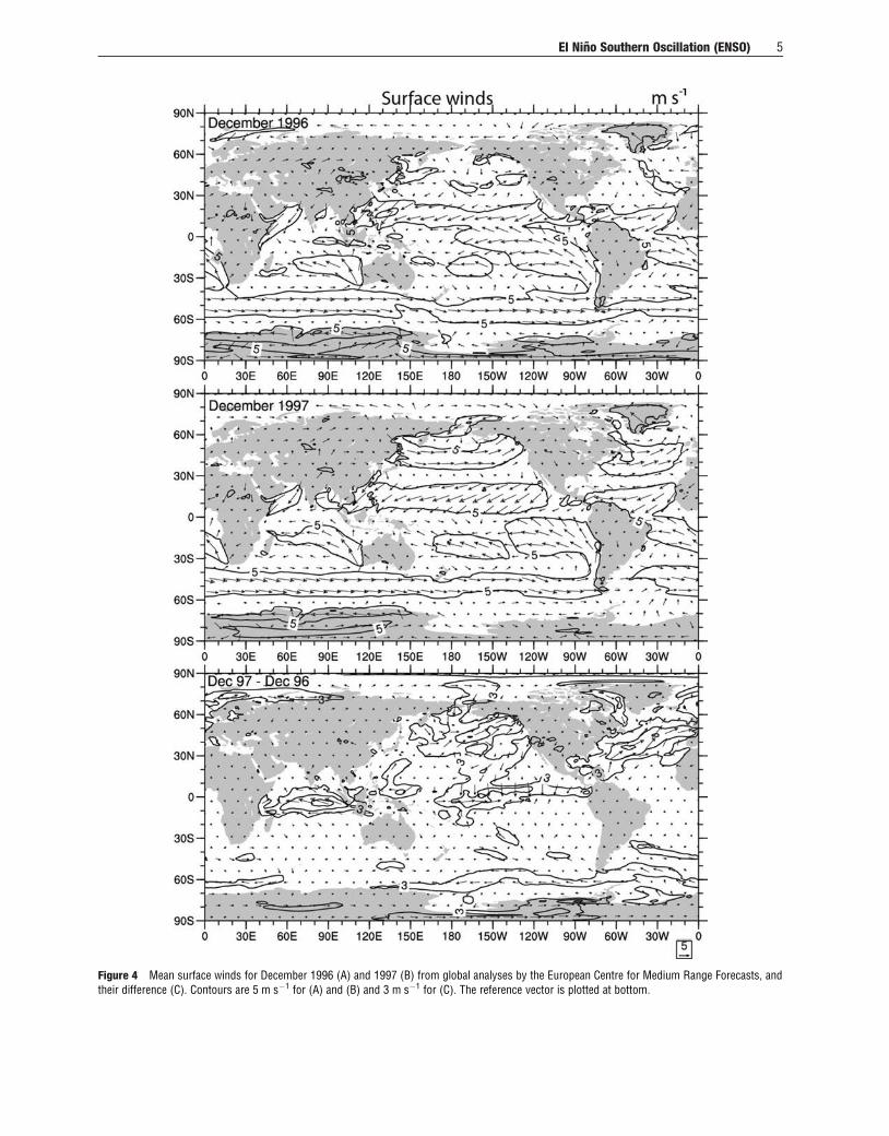
Figure 4 Mean surface winds for December 1996 (A) and 1997 (B) from global analyses by the European Centre for Medium Range Forecasts, andtheir difference (C). Contours are 5 m s�1 for (A) and (B) and 3 m s�1 for (C). The reference vector is plotted at bottom.

El Nino Southern Oscillation (ENSO) 5

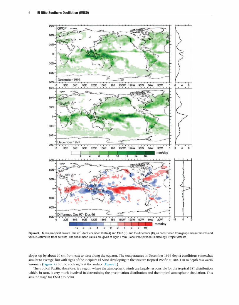
Figure 5 Mean precipitation rate (mm d�1) for December 1996 (A) and 1997 (B), and the difference (C), as constructed from gauge measurements andvarious estimates from satellite. The zonal mean values are given at right. From Global Precipitation Climatology Project dataset.

6 El Nino Southern Oscillation (ENSO)

slopes up by about 60 cm from east to west along the equator. The temperatures in December 1996 depict conditions somewhat

similar to average, but with signs of the incipient El Nino developing in the western tropical Pacific at 100–150 m depth as a warm

anomaly (Figure 7) but no such signs at the surface (Figure 1).

The tropical Pacific, therefore, is a region where the atmospheric winds are largely responsible for the tropical SST distribution

which, in turn, is very much involved in determining the precipitation distribution and the tropical atmospheric circulation. This

sets the stage for ENSO to occur.

30˚N

15˚N

0˚

15˚S

30˚S120�E 140�E 160�E 180˚ 160�W 140�W 120�W 100�W 80�W

TAO Array

AtlasCurrent meter

Figure 6 A center piece of the Pacific El Nino observing system is an array of buoys in the tropical Pacific moored to the ocean bottom known asthe TAO/Triton (Tropical Atmosphere–Ocean) array. The latter is maintained by a multinational group spearheaded in the United States by NationalOceanic and Atmospheric Administration. Each buoy has a series of temperature measurements on a sensor cable on the upper 500 m of the mooring,and on the buoy itself are sensors for surface wind, sea surface temperature, surface air temperature, humidity, and a transmitter to satellite.Observations are continually made, averaged into hourly values, and transmitted via satellite to centers around the world for prompt processing.Right, an ATLAS (Autonomous Temperature Line Acquisition System) buoy. Courtesy Pacific Marine Environmental Laboratory (NOAA).

0 0

00

001001

100100

002002

200200

003003

300300

004004

400400

005005

500500

Dep

th (m

)

Dep

th (m

)D

epth

(m)

Dep

th (m

)

Means

32 32

28 28

24 24

20 20

16 16

12 12

8 8

4 4

0 0Means

seilamonAseilamonA

12 12

8 8

4 4

0 0

-4 -4

-8 -8

-12 -12

140˚ E 140˚ E180 180140˚ W 140˚ W100˚ W 100˚ W

(b)

(d)(c)

(a)

28

1412

10

0

0

0

2

1

_ 3_5

2 3 4 5 610

_1

1

0

0

10

12

14

28

Figure 7 Zonal cross sections along the equator across the Pacific Ocean (2�N to 2�S) from the TAO array temperatures for December 1996 (A, C)and 1997 (B, D). (A, B) total field; (C, D) anomalies. Contours every 1 �C.

El Nino Southern Oscillation (ENSO) 7

Mechanisms of ENSO

Most of the interannual variability in the atmosphere in the tropics and a substantial part of the variability over the extratropics is

related and tied together through ENSO. ENSO is a natural phenomenon arising from coupled interactions between the

atmosphere and the ocean in the tropical Pacific Ocean, and there is good evidence from cores of coral and glacial ice in the

Andes that it has been going on for millennia.

During El Nino, the tradewinds weaken (Figure 4) which causes the thermocline to become shallower in the west and deeper in

the eastern tropical Pacific (Figure 7), while sea level falls in the west and rises in the east by as much as 25 cm as warm waters surge

eastward along the equator. Equatorial upwelling decreases or ceases and so the cold tongue weakens or disappears (e.g., as in

December 1997, Figure 1) and the nutrients for the food chain are substantially reduced. The resulting increase in sea temperatures

(e.g., Figure 1) warms and moistens the overlying air so that convection breaks out, and the convergence zones and associated

rainfall move to a new location with a resulting change in the atmospheric circulation (Figure 5). A further weakening of the surface

trade winds completes the positive feedback cycle leading to an El Nino event. The shifts in the location of the organized rainfall in

the tropics and the latent heat released alters the heating patterns of the atmosphere. Somewhat like a rock in a stream of water, the

8 El Nino Southern Oscillation (ENSO)

anomalous heating sets up waves in the atmosphere that extend into midlatitudes altering the winds and changing the jet stream

and storm tracks (e.g., Figure 8). Note especially the strong westerly jets in the Pacific of both hemispheres, and in the Northern

(winter) Hemisphere the jet stream in December 1997 extends into California and across the southern United States, carrying with

it disturbances that result in extensive rains. Weaker westerlies exist farther north and so the overall storm track shifts towards the

equator in the Pacific.

Although the El Ninos and La Ninas are often referred to as ‘events’ which last a year or so, ENSO is oscillatory in nature. The

ocean is a source of moisture and its enormous heat capacity acts as the flywheel that drives the system through its memory of the

past, resulting in an essentially self-sustained sequence in which the ocean is never in equilibrium with the atmosphere. The

amount of warm water in the tropics builds up prior to and is then depleted during El Nino. During the cold phase with relatively

clear skies, solar radiation heats up the tropical Pacific Ocean, the heat is redistributed by currents, with most of it being stored in

the deep warm pool in the west or off the equator such as at about 10 or 20�N. During El Nino, heat is transported out of the tropics

within the ocean toward higher latitudes in response to the changing currents, and increased heat is released into the atmosphere

mainly in the form of increased evaporation, thereby cooling the ocean. Added rainfall contributes to a general warming of the

global atmosphere that peaks a fewmonths after a strong El Nino event. It has therefore been suggested that the time scale of ENSO

is determined by the time required for an accumulation of warm water in the tropics to essentially recharge the system, plus the

time for the El Nino itself to evolve. Thus a major part of the onset and evolution of the events is determined by the history of what

has occurred one to two years previously. This also means that the future evolution is predictable for several seasons in advance.

Interannual Variations in Climate

The subsurface temperature anomalies which eventually developed into the 1997–98 El Nino were traceable at least from about

September 1996 on the equator in the far western Pacific. However, positive subsurface temperature anomalies in the upper

100–200 m in the far western Pacific exceeded 1 �C for all the months of 1996, and so this was not a sufficient predictor.

By December 1996 (Figure 7) subsurface temperature anomalies in the vicinity of the equator had grown to exceed 2.5 �C at

150 m depth and the warm anomaly extended from at least 140�E (the westernmost buoy) to 140�W. However, conditions were

still below normal in the eastern Pacific. By December 1997, the subsurface warm anomaly had progressed eastward and amplified

to produce positive anomalies exceeding 11 �C (Figure 7) at about 100 m depth, accompanying the surface SST anomalies

exceeding 5 �C (Figure 1). Also note, however, in December 1997 the subsequent cold anomaly of over 5 �C in the western

equatorial Pacific near 150 m depth, as the warm pool was displaced into the central Pacific. The warm pool in the east continued

to diminish with time as the cold anomaly intensified and subsequently spread all the way across the Pacific as part of the signature

of the La Nina that began about June 1998, although it did not develop to a fully fledged event until later in the year. A key aspect of

these changes was the obvious loss of heat content throughout the equatorial Pacific beginning late 1997 and continuing through

1998.

The evolution of SST in several recent ENSO events after 1950 is shown in Figure 9 for two regions. The region of the Pacific

Ocean which is most involved in ENSO is the central equatorial Pacific, especially the area 5�N to 5�S, 170�E to 120�W, whereas the

traditional El Nino region is along the coast of South America. The latter is less important for the global changes in weather patterns

but is certainly important locally. Variations in both regions are closely related but differ in detail from event to event in relative

amplitudes and sequencing. For SSTs, the departure from average required for an El Nino is 0.5 �C over the central Pacific region,

which is large enough to cause perceptible effects in Pacific rim countries. Larger El Nino events have traceable influences over more

extensive regions and even globally.

The ENSO events clearly identifiable in Figure 9 since 1950 occurred in 1951, 1953, 1957–58, 1963, 1965, 1969, 1972–73,

1976–77, 1982–83, 1986–87, 1990–95, 1997–98, 2002–03, 2004–05, 2006–07 and 2009–10. The 1990–95 event might also be

considered three modest events where the conditions in between failed to return to below normal so that they merged together.

Worldwide climate anomalies lasting several seasons have been identified with all of these events. The 1997–98 event has the

biggest SST departures on record, but for the SOI, the El Nino event of 1982–83 still holds the record (Figure 3).

Each El Nino event has its own character. In the El Nino winters of 1992–93, 1994–95, and 1997–98, southern California was

battered by storms and experienced flooding and coastal erosion (in part aided by the high sea levels). However, in more modest El

Ninos (e.g., 1986–87 and 1987–88 winters) California was more at risk from droughts. Because of the enhanced activity in the

Pacific and the changes in atmospheric circulation throughout the tropics, there is a decrease in the number of tropical storms and

hurricanes in the tropical Atlantic during El Nino. A good example is 1997, one of the quietest Atlantic hurricane seasons on record,

whereas the 1990–95 and 1997–98 El Ninos terminated before the 1995 and 1998 hurricane seasons which unleashed the Atlantic

storms and placed those seasons among the most active on record.

The SO has global impacts, however; the connections to higher latitudes (known as teleconnections) tend to be strongest in the

winter of each hemisphere and feature alternating sequences of high and low pressures accompanied by distinctive wave patterns in

the jet stream (Figure 8) and storm tracks in mid-latitudes. Although warming is generally associated with El Nino events in the

Pacific and extends, for instance, into western Canada and Alaska, cool conditions typically prevail over the North and South

Pacific Oceans. To a first approximation, reverse anomaly patterns occur during the La Nina phase of the phenomenon.

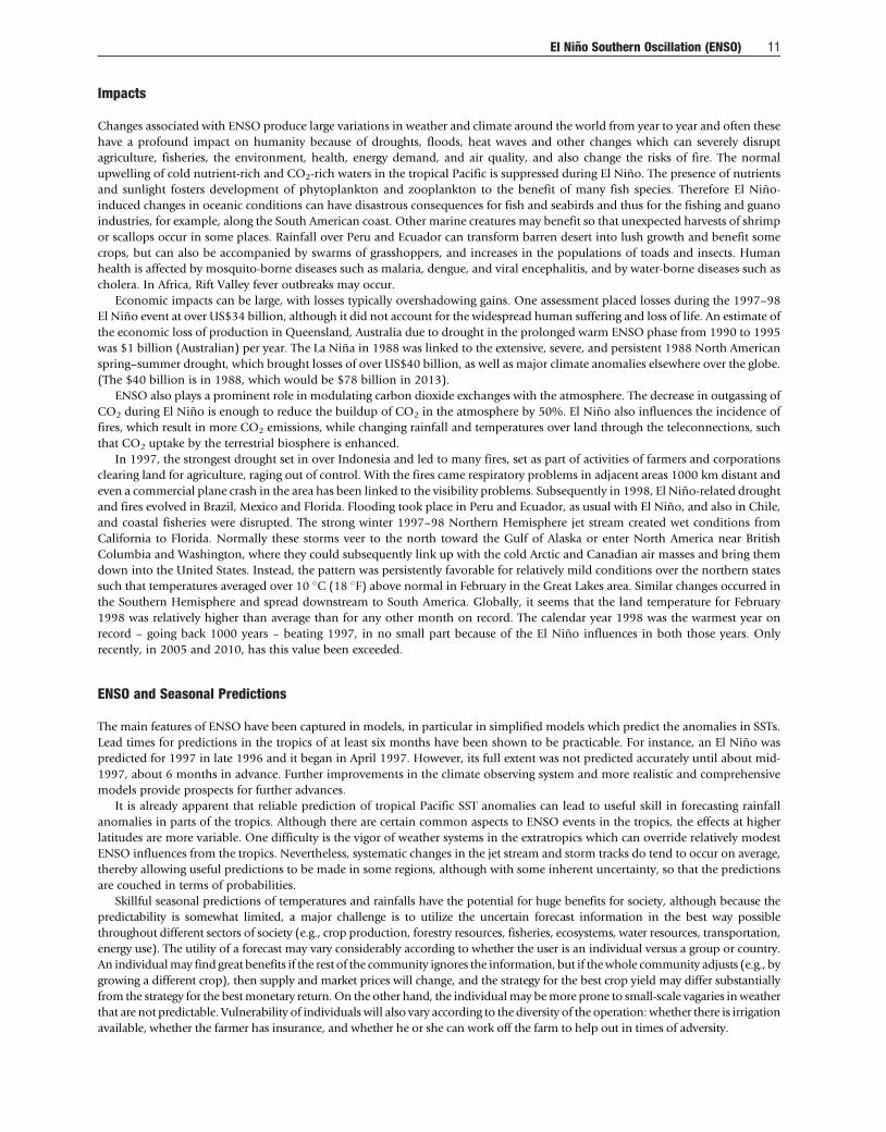
The prominence of the SO has varied throughout the last century (Figure 10). Very slow long-term (decadal) variations are

present; for instance SOI values are mostly below the long-term mean from 1976 to 1998. This accompanies the generally above

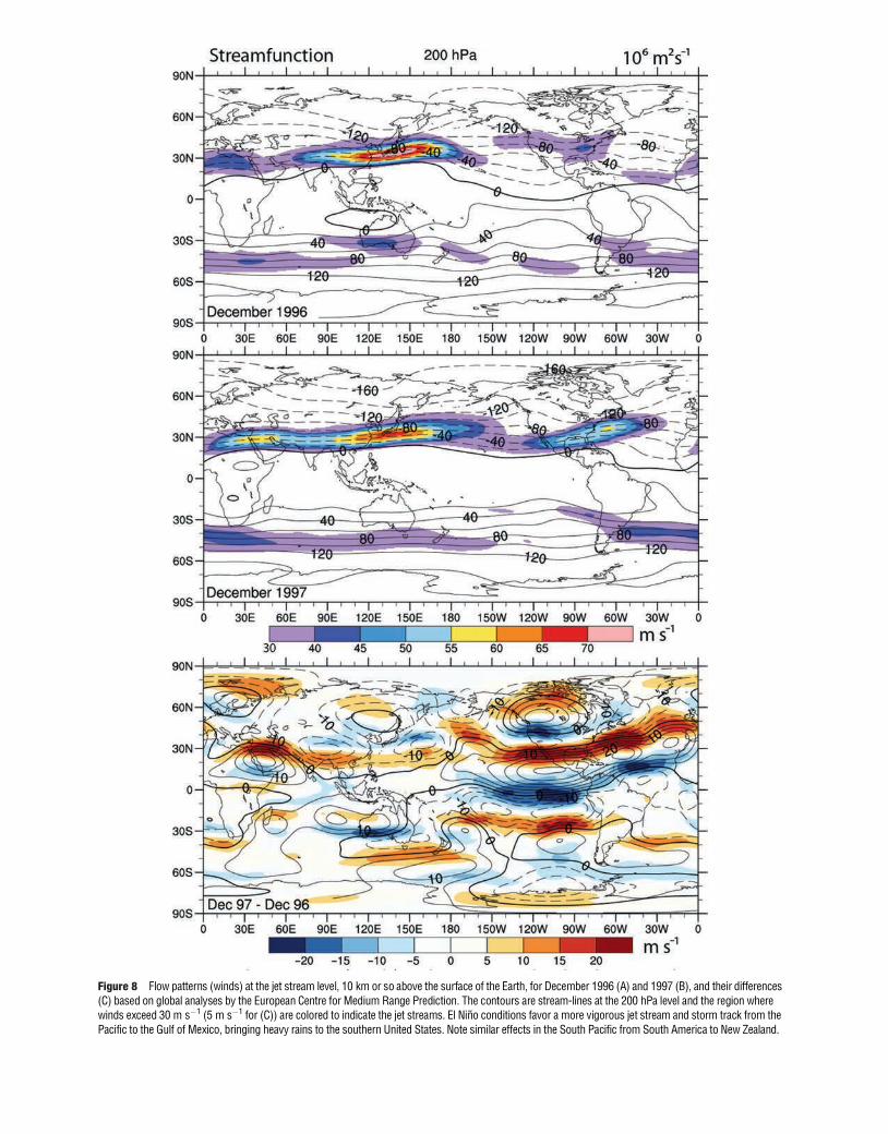
Figure 8 Flow patterns (winds) at the jet stream level, 10 km or so above the surface of the Earth, for December 1996 (A) and 1997 (B), and their differences(C) based on global analyses by the European Centre for Medium Range Prediction. The contours are stream-lines at the 200 hPa level and the region wherewinds exceed 30 m s�1 (5 m s�1 for (C)) are colored to indicate the jet streams. El Nino conditions favor a more vigorous jet stream and storm track from thePacific to the Gulf of Mexico, bringing heavy rains to the southern United States. Note similar effects in the South Pacific from South America to New Zealand.

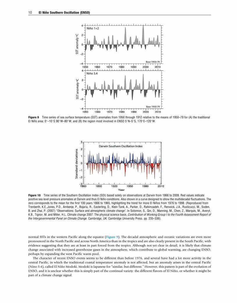
Figure 9 Time series of sea surface temperature (SST) anomalies from 1950 through 1912 relative to the means of 1950–79 for (A) the traditionalEl Nino area: 0�–10�S 90�W–80�W, and (B) the region most involved in ENSO 5�N–5�S, 170�E–120�W.

Figure 10 Time series of the Southern Oscillation Index (SOI) based solely on observations at Darwin from 1866 to 2009. Red values indicatepositive sea level pressure anomalies at Darwin and thus El Nino conditions. Also shown in a curve designed to show the multidecadal fluctuations. Thezero corresponds to the mean for the first 100 years 1866 to 1965, highlighting the trend for more El Ninos from 1976 to 1998. (Reproduced fromTrenberth, K.E.,Jones, P.D., Ambenje, P., Bojariu, R., Easterling, D., Klein Tank, A., Parker, D., Rahimzadeh, F., Renwick, J.A., Rusticucci, M., Soden,B. and Zhai, P. (2007) “Observations: Surface and atmospheric climate change". In Solomon, S., Qin, D., Manning, M., Chen, Z., Marquis, M., Averyt,K.B., Tignor, M. and Miller, H.L. Climate change 2007: The physical science basis. Contribution of Working Group I to the Fourth Assessment Report ofthe Intergovernmental Panel on Climate Change. Cambridge, UK: Cambridge University Press. pp. 235–336).

10 El Nino Southern Oscillation (ENSO)

normal SSTs in the western Pacific along the equator (Figure 9). The decadal atmospheric and oceanic variations are even more

pronounced in the North Pacific and across North America than in the tropics and are also clearly present in the South Pacific, with

evidence suggesting that they are at least in part forced from the tropics. Although not yet clear in detail, it is likely that climate

change associated with increased greenhouse gases in the atmosphere, which contribute to global warming, are changing ENSO,

perhaps by expanding the west Pacific warm pool.

The character of recent ENSO events seems to be different than before 1976, and several have had a lot more activity in the

central Pacific, in which the traditional coastal temperature anomaly is not affected, but an anomaly arises in the central Pacific

(Nino 3.4), called El Nino Modoki. Modoki is Japanese for “similar, but different.” However, this pattern is part of the evolution of

ENSO, and it is unclear whether this is simply part of the continual variety: the different flavors of El Nino, or whether it might be

part of a climate change signal.

El Nino Southern Oscillation (ENSO) 11

Impacts

Changes associated with ENSO produce large variations in weather and climate around the world from year to year and often these

have a profound impact on humanity because of droughts, floods, heat waves and other changes which can severely disrupt

agriculture, fisheries, the environment, health, energy demand, and air quality, and also change the risks of fire. The normal

upwelling of cold nutrient-rich and CO2-rich waters in the tropical Pacific is suppressed during El Nino. The presence of nutrients

and sunlight fosters development of phytoplankton and zooplankton to the benefit of many fish species. Therefore El Nino-

induced changes in oceanic conditions can have disastrous consequences for fish and seabirds and thus for the fishing and guano

industries, for example, along the South American coast. Other marine creatures may benefit so that unexpected harvests of shrimp

or scallops occur in some places. Rainfall over Peru and Ecuador can transform barren desert into lush growth and benefit some

crops, but can also be accompanied by swarms of grasshoppers, and increases in the populations of toads and insects. Human

health is affected by mosquito-borne diseases such as malaria, dengue, and viral encephalitis, and by water-borne diseases such as

cholera. In Africa, Rift Valley fever outbreaks may occur.

Economic impacts can be large, with losses typically overshadowing gains. One assessment placed losses during the 1997–98

El Nino event at over US$34 billion, although it did not account for the widespread human suffering and loss of life. An estimate of

the economic loss of production in Queensland, Australia due to drought in the prolonged warm ENSO phase from 1990 to 1995

was $1 billion (Australian) per year. The La Nina in 1988 was linked to the extensive, severe, and persistent 1988 North American

spring–summer drought, which brought losses of over US$40 billion, as well as major climate anomalies elsewhere over the globe.

(The $40 billion is in 1988, which would be $78 billion in 2013).

ENSO also plays a prominent role in modulating carbon dioxide exchanges with the atmosphere. The decrease in outgassing of

CO2 during El Nino is enough to reduce the buildup of CO2 in the atmosphere by 50%. El Nino also influences the incidence of

fires, which result in more CO2 emissions, while changing rainfall and temperatures over land through the teleconnections, such

that CO2 uptake by the terrestrial biosphere is enhanced.

In 1997, the strongest drought set in over Indonesia and led to many fires, set as part of activities of farmers and corporations

clearing land for agriculture, raging out of control. With the fires came respiratory problems in adjacent areas 1000 km distant and

even a commercial plane crash in the area has been linked to the visibility problems. Subsequently in 1998, El Nino-related drought

and fires evolved in Brazil, Mexico and Florida. Flooding took place in Peru and Ecuador, as usual with El Nino, and also in Chile,

and coastal fisheries were disrupted. The strong winter 1997–98 Northern Hemisphere jet stream created wet conditions from

California to Florida. Normally these storms veer to the north toward the Gulf of Alaska or enter North America near British

Columbia and Washington, where they could subsequently link up with the cold Arctic and Canadian air masses and bring them

down into the United States. Instead, the pattern was persistently favorable for relatively mild conditions over the northern states

such that temperatures averaged over 10 �C (18 �F) above normal in February in the Great Lakes area. Similar changes occurred in

the Southern Hemisphere and spread downstream to South America. Globally, it seems that the land temperature for February

1998 was relatively higher than average than for any other month on record. The calendar year 1998 was the warmest year on

record – going back 1000 years – beating 1997, in no small part because of the El Nino influences in both those years. Only

recently, in 2005 and 2010, has this value been exceeded.

ENSO and Seasonal Predictions

The main features of ENSO have been captured in models, in particular in simplified models which predict the anomalies in SSTs.

Lead times for predictions in the tropics of at least six months have been shown to be practicable. For instance, an El Nino was

predicted for 1997 in late 1996 and it began in April 1997. However, its full extent was not predicted accurately until about mid-

1997, about 6 months in advance. Further improvements in the climate observing system and more realistic and comprehensive

models provide prospects for further advances.

It is already apparent that reliable prediction of tropical Pacific SST anomalies can lead to useful skill in forecasting rainfall

anomalies in parts of the tropics. Although there are certain common aspects to ENSO events in the tropics, the effects at higher

latitudes are more variable. One difficulty is the vigor of weather systems in the extratropics which can override relatively modest

ENSO influences from the tropics. Nevertheless, systematic changes in the jet stream and storm tracks do tend to occur on average,

thereby allowing useful predictions to be made in some regions, although with some inherent uncertainty, so that the predictions

are couched in terms of probabilities.

Skillful seasonal predictions of temperatures and rainfalls have the potential for huge benefits for society, although because the

predictability is somewhat limited, a major challenge is to utilize the uncertain forecast information in the best way possible

throughout different sectors of society (e.g., crop production, forestry resources, fisheries, ecosystems, water resources, transportation,

energy use). The utility of a forecast may vary considerably according to whether the user is an individual versus a group or country.

An individualmay find great benefits if the rest of the community ignores the information, but if thewhole community adjusts (e.g., by

growing a different crop), then supply and market prices will change, and the strategy for the best crop yield may differ substantially

from the strategy for the bestmonetary return. On the other hand, the individualmay bemore prone to small-scale vagaries inweather

that are not predictable. Vulnerability of individuals will also vary according to the diversity of the operation: whether there is irrigation

available, whether the farmer has insurance, and whether he or she can work off the farm to help out in times of adversity.

12 El Nino Southern Oscillation (ENSO)

Further Reading

Collins M, S-Il An W, Cai A, et al. (2012) The impact of global warming on the tropical Pacific Ocean and El Nino. Nature Geoscience. http://dx.doi.org/10.1038/ngeo868.Glantz MH, Katz RW, and Nicholls N (eds.) (1991) Teleconnections linking world-wide climate anomalies. Cambridge: Cambridge University Press.Glantz MH (2001) Currents of change. Cambridge: Cambridge University Press. ISBN 0-521-78672-X.McPhaden MJ, Lee T, and McClurg D (2011) El Nino and its relationship to changing background conditions in the tropical Pacific Ocean. Geophysical Research Letters

38. http://dx.doi.org/10.1029/2011GL048275, L15709.National Research Council (1996) Learning to predict climate variations associated with El Nino and the southern oscillation: Accomplishments and legacies of the TOGA program.

Washington: National Academy Press.Trenberth KE (1997) The definition of El Nino. Bulletin of the American Meteorological Society 78: 2771–2777.Trenberth KE (1999) The extreme weather events of 1997 and 1998. Consequences 5(1): 2–15.Trenberth KE, et al. (2002) Evolution of El Nino – southern oscillation and global atmospheric surface temperatures. Journal of Geophysical Research 107(D8): 4065. http://dx.doi.org/

10.1029/2000JD000298.Trenberth KE, Jones PD, Ambenje P, et al. (2007) “Observations: Surface and atmospheric climate change” In: Solomon S, Qin D, Manning M, Chen Z, Marquis M, Averyt KB,

Tignor M, and Miller HL (eds.) Climate change 2007: The physical science basis. Contribution of Working Group I to the Fourth Assessment Report of the Intergovernmental Panelon Climate Change, pp. 235–336. Cambridge, UK: Cambridge University Press.

Trenberth KE and Stepaniak DP (2001) Indices of El Nino evolution. Journal of Climate 14(8): 1697–1701.Yeh S-W, Kug J-S, Dewitte B, Kwon M, Kirtman BP, and Jin F-F (2009) El Nino in a changing climate. Nature 461: 511–514.