Embed Size (px)
Citation preview

Sensors & Software Inc.1091 Brevik PlaceMississauga, ON L4W 3R7Canada
Phone: (905) 624-8909Fax: (905) 624-9365E-mail: [email protected] Site: www.sensoft.on.ca
Technical Manual 30 Copyright 2001 Sensors & Software Inc.
D#: 01-0117-00
EKKO-for-DVL
User’s GuideVersion 1.0
pulseEKKO 100


Table of Contents 1 Overview ...........................................................................................................11
2 System Assembly and Startup ...................................................................122.1 Antenna Assembly .......................................................................................22.2 Connecting up the Radar..............................................................................32.3 Adding Optional Items.................................................................................5
2.3.1 Electrical Remote Trigger and Beeper Unit ................................................52.3.2 Fiber Optic Remote Trigger and Beeper Unit .............................................52.3.3 Odometer ............................................................................................72.3.4 High Speed Data Acquisition ..................................................................8
2.4 Starting up the System .................................................................................92.4.1 Digital Video Logger.............................................................................92.4.2 Main Menu........................................................................................102.4.3 Using the Software Menus....................................................................10
3 Setting Data Collection Parameters ........................................................123.1 Overview....................................................................................................13
3.1.1 Survey Type ......................................................................................133.1.2 Operating Mode..................................................................................133.1.3 Step Size ...........................................................................................133.1.4 Antenna Separation .............................................................................143.1.5 Frequency .........................................................................................153.1.6 Time Window ....................................................................................153.1.7 Sampling Interval ...............................................................................163.1.8 Number of Stacks ...............................................................................16
3.2 Defaults ......................................................................................................173.3 Exit.............................................................................................................183.4 Field Line ...................................................................................................18
3.4.1 Return ..............................................................................................193.4.2 Mode................................................................................................193.4.3 Distance Units....................................................................................193.4.4 Antenna Separation .............................................................................193.4.5 Survey Type ......................................................................................193.4.6 Pause Trc ..........................................................................................203.4.7 Start Pos............................................................................................203.4.8 Step Size ...........................................................................................203.4.9 StrtDelay...........................................................................................203.4.10 Delay................................................................................................20
3.5 Gains ..........................................................................................................203.5.1 AGC Gain .........................................................................................213.5.2 SEC Gain ..........................................................................................233.5.3 Constant Gain ....................................................................................263.5.4 Autogain ...........................................................................................27
3.6 Job..............................................................................................................273.6.1 Set Directory......................................................................................273.6.2 Pulser Voltage....................................................................................283.6.3 Return ..............................................................................................28
3.7 Layout ........................................................................................................283.7.1 Baud ................................................................................................28
3.7.2 Graph ...............................................................................................283.7.3 Port ..................................................................................................283.7.4 Screen ..............................................................................................293.7.5 Trace ................................................................................................29
3.8 Options.......................................................................................................303.8.1 Depth Axis ........................................................................................303.8.2 Correction .........................................................................................303.8.3 Down the Trace Filter ..........................................................................323.8.4 Background Subtract Filter ...................................................................333.8.5 Optimize Color Plot ............................................................................34
3.9 System........................................................................................................343.9.1 Antenna Frequency .............................................................................343.9.2 Time Window ....................................................................................353.9.3 Sampling Interval ...............................................................................353.9.4 No. Stacks .........................................................................................363.9.5 Return ..............................................................................................36
3.10 Velocity......................................................................................................36
4 Data Collection ..............................................................................................1384.1 Graph .........................................................................................................38
4.1.1 Graph Screen .....................................................................................384.1.2 Error Messages...................................................................................394.1.3 Timezero Adjustment ..........................................................................394.1.4 Data Collection Modes.........................................................................404.1.5 Graph Data Menu ...............................................................................40
4.2 Collect ........................................................................................................414.2.1 Do Not Save Data ...............................................................................414.2.2 Input File Name..................................................................................414.2.3 Data Collection ..................................................................................414.2.4 Data Collection Sequence.....................................................................434.2.5 Odometer Data Acquisition...................................................................444.2.6 Collect Data Menu ..............................................................................44
4.3 Replay ........................................................................................................464.4 Error Messages ..........................................................................................47
4.4.1 Radar System Errors............................................................................474.4.2 File Related Errors ..............................................................................48
5 Troubleshooting ............................................................................................1495.1 System Console Error ................................................................................495.2 DVL Problems ...........................................................................................505.3 Receiver Error............................................................................................505.4 Transmitter Problem: No Signal on Screen ...............................................525.5 Timezero Drifting ......................................................................................525.6 Timezero Jitter ...........................................................................................535.7 Battery Voltage Check...............................................................................535.8 Cannot Continue in Step Mode..................................................................53
6 File Management ..........................................................................................1546.1 File Management Menus ...........................................................................546.2 Transferring Data Files to an External PC using the PXFER Program .....54
6.2.1 Connecting the Digital Video Logger to an External Computer ....................54

6.2.2 Installing and Running the PXFER.EXE Program .....................................556.2.3 Transferring Data Files ........................................................................566.2.4 Parallel Port not bi-directional Error .......................................................56
6.3 Viewing Data Files on the External PC .....................................................576.4 Deleting Data Files from the DVL ............................................................57
7 Care and Maintenance ...............................................................................1587.1 General.......................................................................................................587.2 Radar Unit..................................................................................................587.3 Antenna Electronics Connection Pins........................................................587.4 Battery Power Requirements .....................................................................587.5 Transmitter and Receiver Battery Maintenance ........................................587.6 Testing Batteries ........................................................................................597.7 Fiber Optics Cables....................................................................................607.8 Fiber Optics Cable Repair..........................................................................60
8 Helpful Hints .................................................................................................1628.1 Handling Fiber Optic Cables .....................................................................628.2 Connecting the Fiber Optics ......................................................................628.3 Console Location .......................................................................................628.4 Setting up for Reflection (Profiling) Mode................................................628.5 Aliasing the Data .......................................................................................638.6 Performing A CMP....................................................................................638.7 Setup for Transillumination Surveys .........................................................648.8 Batteries .....................................................................................................658.9 Measuring Position ....................................................................................658.10 Data Files ...................................................................................................658.11 Spares.........................................................................................................65
Appendix A: Excerpts from the HP Fiber Optics Handbook
Appendix B: Quick Guide to Data Collection
Appendix C:GPR Signal Processing Artifacts
Appendix D:Data File Formats
Appendix E:Health & Safety


EKKO-for-DVL 1-Overview
1 OverviewThis manual describes how to set up and run a pulseEKKO 100 Ground Penetrating Radar (GPR) system connected to a Digital Video Logger (DVL) for data display and storage.
System Assembly Section 2 on page 2 discusses in detail the step by step procedure for& Startup: assembling the pulseEKKO 100 system and connecting it to the DVL. It also
describes how to start up the DVL and maneuver around the menus.
Setting Data Collection Section 3 on page 12 covers the procedure for selecting appropriateParameters: data collection parameters. Although every effort has been made to make the soft-
ware as transparent and user friendly as possible, this section explains in greater detail each of the options and menu items in the data collection program.
To get up and running quickly see Appendix B:Quick Guide to Data Collection.
Data Collection: Section 4 on page 38 describes running the radar system and collecting data.
Troubleshooting: Section 5 on page 49 presents some simple steps the user should go through when things do not work as they should.
File Management: Section 6 on page 54 describes how to transfer data from the DVL to a PC and how to delete files and directories from the DVL.
Care and Maintenance: Section 7 on page 58 discusses procedures for the care and maintenance of your pul-seEKKO system.
Helpful Hints: Based on years of experience, Section 8 lists some helpful hints to help make data collection and field operations run as smooth as possible.
Users should read Sensors & Software’s statement on issues regarding health and safety in Appendix E:Health & Safety.
1

2-System Assembly and Startup EKKO-for-DVL
2 System Assembly and StartupThe modular design of the pulseEKKO 100 GPR makes the system very flexible and readily field-portable. There are four essential components to the radar system: the control or console unit, the transmitter assembly, the receiver assembly and the Digital Video Logger (DVL). The transmitter and receiver assemblies are connected to the console unit via appropriate fiber optics cables and the console is connected to the DVL via a RS232 cable (Figure 2-1). This section discusses the detailed steps to follow to assemble the whole pulseEKKO 100 system.
Figure: 2-1
2.1 Antenna Assembly
The procedures for assembling the transmitter and receiver antennas are identical. A detailed diagram of this assembly can be found in Figure 2-2. The assembly steps are as follows:
a) Check the two male brass antenna connector pins for damage; replace if necessary. Insert the pins into the two threaded holes in the center of the antennas. Tighten the pins finger-tight. DO NOT APPLY UNDUE FORCE !
b) Insert and tighten the two female brass antenna sockets into the bottom of the transmitter and receiver electronic boxes. Tighten the sockets finger-tight. DO NOT APPLY UNDUE FORCE !
c) Attach the antenna mounting block to the antenna by using the flathead screwdriver to tighten the 4 (four) quarter-turn fasteners, ensuring that the male brass antenna pins protrude up the center holes of the mounting blocks. Quarter-turn fasteners work by aligning the screw in the socket and the pressing
2

EKKO-for-DVL 2-System Assembly and Startup
downward and tightening a quarter of a turn. DO NOT APPLY UNDUE FORCE. It is usually best to have all the screws properly aligned in their socket before tightening each one.
d) Carefully place the electronic boxes down onto the mounting block such that both brass pins fully connect. Then use the 2 plastic draw latch connectors to hold the electronics boxes on the mounting block.
e) With the transmitter and receiver power switched OFF, unlatch the 2 battery covers on the sides of the electronics and open. Place one 12-volt battery on each side on the electronics boxes making sure the positive (+) terminal faces inward toward the electronics (the battery only fits properly in this orientation). Close and latch the battery covers. Note that the system will run with only one 12 volt battery but using two batteries is recommended.
f) Attach the adjustable handle to the antenna using the flat head screwdriver to tighten the 4 quarter-turn fasteners as with the mounting block. This handle can then be adjusted for height by loosening the 2 knurled knobs by hand, moving the handle to the desired height and retightening the knobs (Figure 2-2).
Figure: 2-2
2.2 Connecting up the Radar
Once the antennas are assembled, the next step is to connect the antennas to the console and the console to the DVL. Refer to Figure 2-1.
a) Check the fiber optic cables for damage by holding one end towards a light source and looking into the other end. If light is not transmitted through the cable or appears dim, then replace or repair the cable (see the Section 7.8 on page 60 and Appendix A:Excerpts from the HP Fiber Optics Handbook). Inspect the cable for any kinks or signs of damage and, again, repair if necessary.
b) Plug the black end of the single fiber optics cable (or dual fiber optics cable if you are using a remote
3

2-System Assembly and Startup EKKO-for-DVL
trigger or odometer; see below) into the INPUT (black) connector in the transmitter and the other end into the single red receptacle labelled “Transmitter” on the console.
c) Plug the dual fiber optics cable into the receiver, black to black and grey to grey, and the other ends likewise into the double yellow receptacles labelled “Receiver” on the radar console.
d) Using the RS232 cable, connect the console unit (white receptacle) to the serial port on the DVL (the cable will only fit in one of the receptacles on the back of the DVL). It is suggested that these connections be secured with proper screws to prevent accidental disconnection during operation.
e) Connect the DVL to Power Supply Cable to the 9-socket connector on the back of the DVL. Then connect the Power Cable Extension with Alligator Clips to the end of the DVL to Power Supply Cable. The alligator clips can then be connected to a 12 Volt battery. Make sure that the black clip is attached to the negative (-) and the red clip is attached to the positive (+) battery terminals. If the alligator clips are connected to the wrong terminals of the battery, the DVL will not be powered. When the DVL is receiving power the upper red light on the front of the DVL will be illuminated.
Figure: 2-3
f) Turn the transmitter and receiver ON by pressing the button on the top of each unit. The red Power light should come on to indicate that power is being received. If not, check that the batteries inside the Transmitter and Receiver are fully charged and have been inserted the right way.
g) Turn the DVL ON by pressing any button on the front. As the DVL boots up, the lower red light will come on and it will beep until it has fully booted up.
h) Connect the console power supply to the white POWER receptacle and turn power supply ON, if necessary. If a battery cable is being used make sure that the black clip is attached to the negative (-) and the red clip is attached to the positive (+) battery terminals.
i) Before actually storing data, allow the console to run to reach ambient operating temperature. This time varies depending on outside temperature; however, 5 to 10 minutes is generally sufficient.
j) When not collecting data, the transmitter, receiver and console should be turned OFF to increase the life of the batteries.
Note that it is possible for the pulseEKKO 100 console and the DVL to share a common 12 Volt power source like a battery. Simply connect the alligator clips on the Console Power Supply cable and the Power Cable Extension with Alligator Clips to the proper terminals of the battery.
4

EKKO-for-DVL 2-System Assembly and Startup
2.3 Adding Optional Items
2.3.1 Electrical Remote Trigger and Beeper Unit
To connect the electrical remote trigger and beeper unit, connect the cable attached to the unit to the red electrical REMOTE receptacle on the console (Figure 2-4).
Figure: 2-4
During data acquisition, the beeper will emit a beep as data are being collected.
As well, when the radar system is run in Step mode (see Section 3.4.2 on page 19), data acquisition can be controlled using the button on the remote trigger and beeper unit.
2.3.2 Fiber Optic Remote Trigger and Beeper Unit
To attach the Fiber Optic Remote unit to the pulseEKKO 100 deluxe handles, remove the screw near the top of one of the handles. Then attach the two pieces of the handle attachment assembly (Figure 2-5) and replace the screw as shown. Now press the Fiber Optic Remote onto the handle and twist it a quarter-turn into place.
Figure: 2-5
For PVC handles, attach the Fiber Optic Remote to the handle as shown in Figure 2-6.
5

2-System Assembly and Startup EKKO-for-DVL
Figure: 2-6
To connect up the fiber optic remote trigger and beeper unit you should have a dual fiber optic cable for the console to transmitter connection plus a short single fiber optic cable (Figure 2-7). One of the two cables on the dual fiber optic cable will, if the above directions were followed, already be connected from the red transmitter receptacle on the console to the black (INPUT) receptacle on the transmitter.
Figure: 2-7
6
EKKO-for-DVL 2-System Assembly and Startup
The steps necessary to complete the connection of the remote trigger and beeper unit are:
1) The black fiber optic cable of the dual cable connects from the red REMOTE receptacle on the console to the OUTPUT (grey) fiber optic connector on the remote trigger and beeper unit. This connection is necessary for the trigger part of the remote trigger and beeper unit to work.
2) The short single fiber optic cable connects from the INPUT (black) fiber optic connector on the remote trigger and beeper unit to the OUTPUT (grey) receptacle on the transmitter. This connection is necessary for the beeper part of the remote trigger and beeper unit to work.
Note that if you have a pulseEKKO 100 console with a pulseEKKO IV transmitter only connection 1 is necessary.
During data acquisition, the beeper will emit a beep as data are being collected.
As well, when the radar system is run in Step mode (see Section 3.4.2 on page 19), data acquisition can be controlled using the button on the remote trigger and beeper unit.
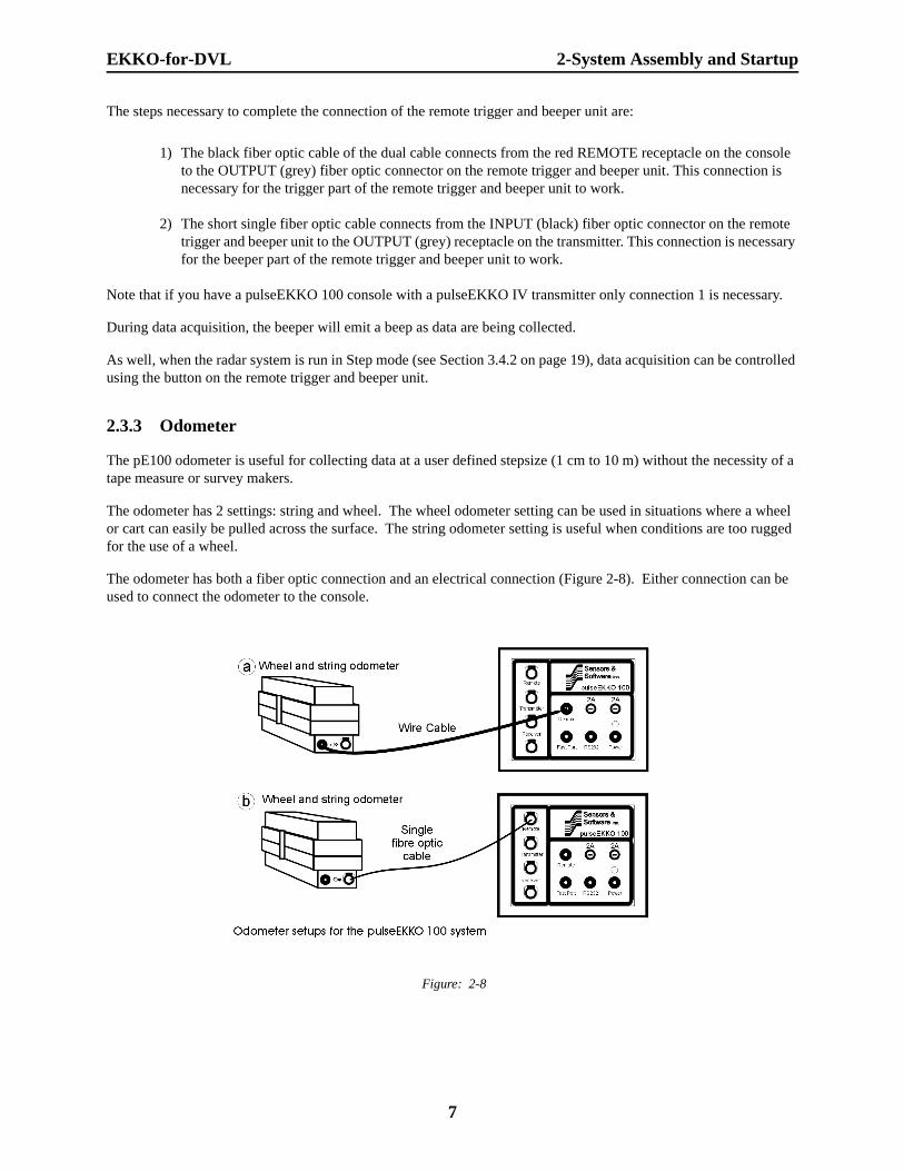
2.3.3 Odometer
The pE100 odometer is useful for collecting data at a user defined stepsize (1 cm to 10 m) without the necessity of a tape measure or survey makers.
The odometer has 2 settings: string and wheel. The wheel odometer setting can be used in situations where a wheel or cart can easily be pulled across the surface. The string odometer setting is useful when conditions are too rugged for the use of a wheel.
The odometer has both a fiber optic connection and an electrical connection (Figure 2-8). Either connection can be used to connect the odometer to the console.
Figure: 2-8
7

2-System Assembly and Startup EKKO-for-DVL
1) Electrical Connection: To connect up the odometer using the electrical connection you should have the proper cable for the console to odometer connection. Connect the cable from the red electrical REMOTE receptacle on the console to the electrical receptacle on the odometer. (Figure 2-8a)
2) Fiber Optic Connection: To connect up the odometer using the fiber optic connection you should have a dual fiber optic cable for the console to transmitter connection. One of the two cables on the dual fiber optic cable will, if the above directions were followed, already be connected from the red transmitter receptacle on the console to the INPUT (black) receptacle on the transmitter. (Figure 2-8b)
To complete the connection of the odometer the black fiber optic cable of the dual cable connects from the red REMOTE receptacle on the console to the grey fiber optic connector on the odometer.
With either of these connections made, when the radar system is run in Step mode (see Section 3.4.2 on page 19), data acquisition is controlled by the odometer.
2.3.4 High Speed Data Acquisition
With normal speed data acquisition, the serial port is used to transfer data from the console to the computer. The High Speed option allows data acquisition speed to be significantly increased by transferring data from the console using both the serial port and the parallel port of the computer.
Figure: 2-9
To assemble the high speed unit:
1) Plug the female end of the fast-port-to-parallel port cable into the male connector (D-9) on the fast port.
2) Plug the male end of the console-to-fast-port cable into the female connector (D-25) on the fast port.
Now the high speed unit is ready to be connected into the radar system:
1) Plug the male end of the fast-port-to-parallel port cable into the parallel port male connector (D-25) on the DVL.
8

EKKO-for-DVL 2-System Assembly and Startup
2) Plug the yellow end of the console-to-fast-port cable into the yellow receptacle on the console.
To ensure that a short circuit does not occur, make these attachments before turning on the power supply to the console and the DVL.
2.4 Starting up the System
2.4.1 Digital Video Logger
Once all the cable connections are made between the Noggin, the Digital Video Logger (DVL) and the battery, the upper red LED light on the DVL panel should be lit. If the battery voltage is low, the light will flash for about 30 seconds and go out. If the light flashes or does not appear, check the connections and make sure the battery is fully charged.
The low voltage indicator can be helpful for identifying when the battery needs to be recharged. If the battery voltage drops too low the DVL will cease to operate.
The front of the DVL is shown in Figure 2-10. To start the system, press any button on the front panel. The DVL will begin to beep indicating it is booting up. The lower red LED on the front panel should illuminate.
Figure: 2-10 Digital Video Logger (DVL) face
The water-resistant membrane keypad has a number of buttons that can be pressed to perform various tasks. Note that the buttons on the membrane keypad sometimes need to be pressed hard to register.
Menu Buttons: The yellow buttons labelled 1 to 8 correspond to menu choices that appear listed on the screen or along the bottom of the screen when the Digital Video Logger is turned on.
In addition, there are two general-purpose buttons labeled A and B. All buttons are DVL application dependent and roles change. The operation will be self-explanatory from the display screen.
Screen: The DVL screen is a grayscale LCD selected for its wide temperature range and visibility in sunlight. Visibility can be a major problem with viewing GPR data displays outdoors and considerable effort has been expended on getting a readily visible outdoor display.
Brightness: The yellow Brightness control arrows are used to increase and decrease the screen brightness. For example, increasing the Brightness setting may improve the visibility of the screen when outside on a sunny day. Note, however, that increasing the screen brightness also increases battery consumption so don't use a bright screen unless necessary.
9

2-System Assembly and Startup EKKO-for-DVL
Contrast: The yellow Contrast control arrows are used to increase and decrease the screen contrast. For example, increasing the Contrast setting may improve the visibility of weaker features on the screen. Adjusting the contrast has little effect on battery consumption.
Temperature sensors within the DVL automatically compensate the screen setting so that manual adjustments of Brightness and Contrast should seldom be needed after initial setup.
2.4.2 Main Menu
Once all components are properly connected, the radar is ready to operate under DVL control. Turn the DVL on by pressing any button on the front. After the DVL boots up the main menu is displayed.
pulseEKKO for DVL
1 - Run pulseEKKO GPR
2 - File Management
5 - Shut Down
26C
12.4V
To setup data collection parameters and begin acquiring data, press button number 1 for Run pulseEKKO GPR. Details about setting data collection parameters are given in Section 3 on page 12. Details about data collection are given in Section 4 on page 38.
Data files collected can be transferred to an external PC and deleted from the DVL using the File Management menu item. File Management can be selected by pressing button 2 from the main menu. Details about using File Management are given in Section 6 on page 54.
The DVL can be shut down by pressing button number 5.
The two numbers displayed in the lower left corner of the main menu are the interval temperature of the DVL in Celcius and the voltage of the power supply running the DVL. When the DVL voltage drops to 10.5 Volts or less, power-related errors will occur with the system and eventually, when the voltage gets too low, the DVL will shut down. If this occurs in the middle of a data file, that file will be lost.
2.4.3 Using the Software Menus
Menu interaction can be done in one of three ways:
If the menu item has a number listed beside it, that menu item can be selected by pressing the corresponding button number on the DVL. For example, in the above menu, pressing the number 1 will select the menu for running a pulseEKKO GPR system.
1) On a menu with items that are not numbered, one of the menu items will be highlighted (in reverse video) to indicate that it is the current choice. Other items can be highlighted by using the left (), right, up or down arrow key. The button immediately below the arrow should be pressed to move the highlighted menu item in that direction. Once the menu item is highlighted, it can be selected by pressing the button under the Enter option. In this way the user can get move down through different menu levels. Pressing the button under ESC (Escape) will take the user up to the previous menu level.
10

EKKO-for-DVL 2-System Assembly and Startup
2) If data entry is required (for example, when a number needs to be filled into a field), the available field length is shown highlighted. There may or may not already be a current value in the field. As well, a series of numbers like +0.1, +1, +10, and +100 or -0.1, -1, -10 and -100 appears on the bottom of the screen. The user can change the numeric value by selecting the button to increment or decrement the current value by the displayed amount. For example, if the current value is 100.0 and the user wants to change it to 456.3, pressing the button corresponding to +100 three times will increment the value to 400.0. Then pressing the button corresponding to +10 five times will increment the value to 450.0. Then pressing the button corresponding to +1 six times will increment the value to 456.0. Finally, pressing the button corresponding to +0.1 three times will increment the value to the 456.3.
3) To decrement the values using negative values press the button under +/- to toggle the values from positives to negatives.
4) The above explanation may sound complicated but having used it a few times, the whole procedure will become intuitive.
11
3-Setting Data Collection Parameters EKKO-for-DVL
3 Setting Data Collection ParametersThe RUN program is used to set up the data acquisition parameters and collect data. From the main menu select Run pulseEKKO GPR. The next menu gives you a choice of RUN programs including pE100.
The pE100 RUN program is for normal or high speed data collection. For normal data collection, data transfer occurs through the serial port only. For high speed data collection, data transfer occurs through both the serial port and the parallel port.
Note that the high speed parallel port interface is optional hardware that is not present all pulseEKKO systems. If this hardware is not available or not desired, it can be disabled under Layout - Port (see Section 3.7.3 on page 28).
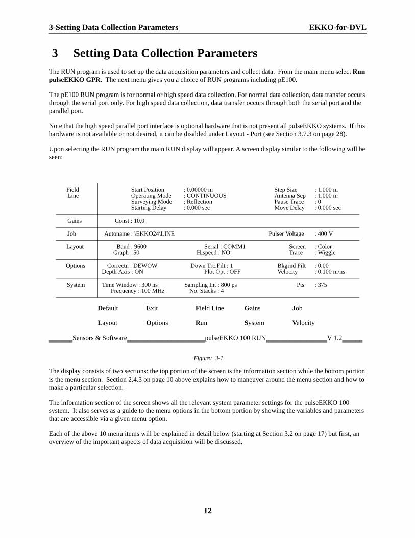
Upon selecting the RUN program the main RUN display will appear. A screen display similar to the following will be seen:
Default Exit Field Line Gains Job
Layout Options Run System Velocity
_______Sensors & Software_______________________pulseEKKO 100 RUN__________________V 1.2______
Figure: 3-1
The display consists of two sections: the top portion of the screen is the information section while the bottom portion is the menu section. Section 2.4.3 on page 10 above explains how to maneuver around the menu section and how to make a particular selection.
The information section of the screen shows all the relevant system parameter settings for the pulseEKKO 100 system. It also serves as a guide to the menu options in the bottom portion by showing the variables and parameters that are accessible via a given menu option.
Each of the above 10 menu items will be explained in detail below (starting at Section 3.2 on page 17) but first, an overview of the important aspects of data acquisition will be discussed.
FieldLine
Start Position Operating ModeSurveying ModeStarting Delay
: 0.00000 m: CONTINUOUS: Reflection: 0.000 sec
Step SizeAntenna SepPause TraceMove Delay
: 1.000 m: 1.000 m: 0: 0.000 sec
Gains Const : 10.0
Job Autoname : \EKKO24\LINE Pulser Voltage : 400 V
Layout Baud : 9600Graph : 50
Serial : COMM1Hispeed : NO
Screen Trace
: Color: Wiggle
Options Correctn : DEWOWDepth Axis : ON
Down Trc.Filt : 1Plot Opt : OFF
Bkgrnd FiltVelocity
: 0.00: 0.100 m/ns
System Time Window : 300 nsFrequency : 100 MHz
Sampling Int : 800 psNo. Stacks : 4
Pts : 375
12

EKKO-for-DVL 3-Setting Data Collection Parameters
3.1 Overview
To run the system, some key parameters have to be set. These are discussed in this section. More detail on individual menu items follow in subsequent sections.
The most important parameters to set for a successful GPR survey are:
3.1.1 Survey Type
Ground penetrating radar has been used in many different survey modes to gather information. Three of the more common modes are:
a) Reflection mode, which is by far the most common mode used to map underlying stratigraphy, (see Fig-ure 8-1 in Section 8.4 on page 62).
b) CMP (Common Mid Point) or WARR (Wide Angle Reflection and Refraction), useful in deducing information on wave propagation velocity versus depth (see Figure 8-3 in Section 8.6 on page 63), and
c) Transillumination where the transmitting and receiving antennas are situated at opposite sides of a partition to study the transmission properties of the dividing material (See Figure 8-4 in Section 8.7 on page 64).
d) These three choices are listed under Field Line - Survey Type (see Section 3.4.5 on page 19).
3.1.2 Operating Mode
When collecting data, the pulseEKKO 100 can be setup to run in one of three operating modes:
a) continuous mode, where the system automatically collects data at regular, user-determined time inter-vals. This mode is good for surveys in flat, unobstructed terrain where antennas can be moved easily. For the position of each measurement point, the system assumes the operator has moved the antennas one stepsize along the survey line.
b) step mode, where the user controls when the system collects data by pressing the B button on the DVL, an external trigger button or using an odometer. This mode is good for surveying in difficult terrain where antennas cannot be moved easily or at regular time intervals. For the position of each measurement point, the system assumes the operator has moved the antennas one stepsize along the survey line. This is also the mode to select when an odometer is being used to trigger the system at specific distance intervals.
c) free-running, is similar to continuous in that the system automatically collects data at regular, user-defined time intervals. However, a stepsize of 1.0 is assumed between measurement points so that position values correspond to trace numbers. True position is controlled by the user adding markers at known positions along the survey line.
The mode of operation to use is best determined by the user after examination of the site to assess the ease with which the radar can be moved from position to position.
This parameter is set under Fieldline - Operating Mode (Section 3.4.2 on page 19).
3.1.3 Step Size
To properly resolve subsurface targets spatially, it is important that a proper Step Size (or Station Spacing) be selected. Too coarse a Step Size may result in missed subsurface targets while too fine a Step Size will result in large data volumes and slow survey productivity.
13

3-Setting Data Collection Parameters EKKO-for-DVL
Step Size is related to the antenna frequency being used and the RUN program displays a chart under the Fieldline menu item listing appropriate Step Sizes for each of the various pulseEKKO antenna frequencies. This chart is reproduced here:
This parameter is set under Fieldline - Step Size (Section 3.4.8 on page 20).
For a more detailed discussion of selecting Step Size see “Ground Penetrating Radar Survey Design” by Annan and Cosway.
3.1.4 Antenna Separation
As the antennas are moved along a survey line it is important that a separation be maintained between them. When the antennas are mounted on a cart the antenna separation is fixed but when the antennas are free it is usually necessary to have a rope or measuring tape to maintain the proper separation (see Figure 8-1 in Section 8.4 on page 62). Each antenna frequency has a minimum separation which is listed in a chart under the Fieldline menu item.
This chart is reproduced below:
Frequency(MHz)
Maximum StepSize (m)(to avoid aliasing)
12.5 2.0
25 1.0
50 0.5
100 0.25
110 0.25
200 0.10
225 0.10
450 0.05
900 0.02
Frequency(MHz)
Min Antenna Separation(m)
12.5 8
25 4
50 2
100 1
110 1
200 0.5
225 0.5
450 0.25
900 0.17
1200 0.075
14

EKKO-for-DVL 3-Setting Data Collection Parameters
The rule of thumb is that the minimum antenna separation is equal to the antenna length. For example, 100 MHz antennas are 1 metre long and should be kept about 1 metre apart during a survey. If the antenna spacing is too small receiver saturation may occur and data lost due to clipping (see Appendix C:GPR Signal Processing Artifacts for a discussion of this problem).
This parameter is set under Fieldline - Antenna Sep (Section 3.4.4 on page 19).
For a more detailed discussion of selecting Antenna Separation see “Ground Penetrating Radar Survey Design” by Annan and Cosway.
3.1.5 Frequency
Deciding on the antenna frequency to use for a survey is dependent on the objectives of the survey. As frequency decreases the depth of investigation generally increases but spatial resolution decreases. Therefore, the ideal survey will be one that uses the highest frequency that adequately penetrates to the target depth. This is not always easy to determine and often field experimentation with several different frequencies is necessary.
The following table offers a guide to deciding on a frequency. It is based on the assumption that spatial resolution of the target is about 25% of the target depth. The values are based on practical experience and should be used as a quick guide only.
The selected frequency requires that you have the correct antennas connected to the system. The software has no way of checking this!!
This parameter is set under System - Frequency (Section 3.9.1 on page 34).
For a more detailed discussion of selecting frequency see “Ground Penetrating Radar Survey Design” by Annan and Cosway.
3.1.6 Time Window
The time window parameter is very important to set adequately. An entire survey could fail if the window is not sufficiently long enough to sample to the depth of the target. Conversely, too long a time window increases the data volume and decreases productivity. Since the radar system really measures time and survey targets are at a specific depth, an estimate of velocity can be used to relate depth to time and get a good time window value.
Depth(m)
Center Frequency(MHz)
0.5 1000
1.0 500
2.0 200
5.0 100
10 50
30 25
50 10
15
3-Setting Data Collection Parameters EKKO-for-DVL
W = 1.3 x (2 x depth)/velocity
The RUN program under System - Time Window does this calculation automatically based on an input velocity. A value of 0.1 m/ns is a good average value for geologic materials but, if required, a table listing velocities of common geologic materials is listed under the Velocity menu item.
This parameter is set under System - Time Window (Section 3.9.2 on page 35).
3.1.7 Sampling Interval
Another important parameter is the time interval between points on the trace. This parameter is dependent on the frequency of the antennas being used. Higher frequencies need to be sampled at a finer time sampling interval than lower frequencies.
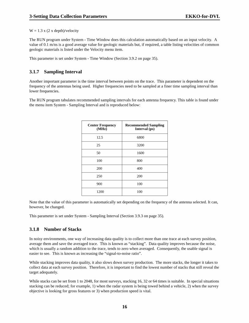
The RUN program tabulates recommended sampling intervals for each antenna frequency. This table is found under the menu item System - Sampling Interval and is reproduced below:
Note that the value of this parameter is automatically set depending on the frequency of the antenna selected. It can, however, be changed.
This parameter is set under System - Sampling Interval (Section 3.9.3 on page 35).
3.1.8 Number of Stacks
In noisy environments, one way of increasing data quality is to collect more than one trace at each survey position, average them and save the averaged trace. This is known as “stacking”. Data quality improves because the noise, which is usually a random addition to the trace, tends to zero when averaged. Consequently, the usable signal is easier to see. This is known as increasing the “signal-to-noise ratio”.
While stacking improves data quality, it also slows down survey production. The more stacks, the longer it takes to collect data at each survey position. Therefore, it is important to find the lowest number of stacks that still reveal the target adequately.
While stacks can be set from 1 to 2048, for most surveys, stacking 16, 32 or 64 times is suitable. In special situations stacking can be reduced; for example, 1) when the radar system is being towed behind a vehicle, 2) when the survey objective is looking for gross features or 3) when production speed is vital.
Center Frequency(MHz)
Recommended Sampling Interval (ps)
12.5 6800
25 3200
50 1600
100 800
200 400
250 200
900 100
1200 100
16

EKKO-for-DVL 3-Setting Data Collection Parameters
This parameter is set under System - No. Stacks (Section 3.9.4 on page 36).
Once these parameters have been set, data collection can begin. First, the system is checked by selecting the Run - Graph mode of operation and finally data are collected with the Run - Collect mode. Data collection is discussed in Section 4 on page 38.
It is important to note that the pulseEKKO 100 system has been designed to try and minimize possible errors by the operator. One important feature of pulseEKKO systems is that they store all the data in its raw format. That is, the gains (see Section 3.5 on page 20) which are applied to the data are only applied to the data displayed on the screen. The data stored in the file has no gain or filtering applied. More details about the actual data stored can be found in the section on formatting in Appendix D:Data File Formats.
The ten RUN menu options will now be discussed in detail.
3.2 Defaults
This option allows the user to load or save default parameter settings for the pulseEKKO 100 radar. These parameter settings includes everything shown in the information section of the screen.
When the data collection program is first run, it loads the parameter settings set the last time the program was run.
Very often, for a given radar job site, a particular set of parameters is used again and again for different profile lines. In such a case, it is very useful to be able to store these parameter settings so that they can be reloaded when needed. This is the function of the Defaults menu option.
Once Defaults is selected, a submenu with two choices is displayed:
____________Defaults__________________________________________________________________________
Load Save Return
_______Sensors & Software_____________________pulseEKKO 100 RUN__________________V 1.2________
Return moves the user back to the main RUN menu.
Load allows the user to load the parameter settings stored in a file that was created previously with the Save option.
Save allows the user to save the current parameter settings in a file named by the user. The file always starts with the prefix DEF and the user selects a number as a suffix, for example DEF78. The user can create up to 100 different default files.
No matter which option (Load or Save) the user chooses, the information that is needed from the user is the file name of the file to be loaded or saved, as the case may be. The following display will be seen (the example is for Load; if Save is chosen, the display is identical, except that instead of Load, the display will read Save):
_______Defaults→Load______________________________________________________________________
Filename:
A for directory
_______Sensors & Software_______________________pulseEKKO 100 RUN__________________V 1.2_______
Pressing A will display a list of all the current default files that reside on the DVL. Once the filename is entered, pressing the ENTER button will Load the parameter settings of the named file. The main menu will reappear, but notice that the parameter settings will be those of the loaded file.
17

3-Setting Data Collection Parameters EKKO-for-DVL
The Save option works in the same way. Please realize that in Save mode, naming an existing default file will overwrite the original.
3.3 Exit
Selecting Exit will exit this program and return the user to the pulseEKKO main menu screen (see Section 2.4.2 on page 10). Exit also serves an important function. Before exiting, the program saves all the current RUN parameters. This process enables the system to start up exactly as before when the RUN program is loaded. Therefore, the user should NOT shut off the DVL without first exiting the program correctly.
3.4 Field Line
Under Field Line are gathered the variables that relate to a given profile line in the field. It is very likely that these variables will change with each profile line, which is why we have grouped them together for convenience. The variables under Job (see Section 3.6 on page 27), on the other hand, are not likely to change from profile line to profile line. There will always be exceptions to this, of course.
Selecting Field Line from the main menu brings up the following screen:
_______Field Line___________________________________________________________________________
Return Mode : CONT Units : metres Separation: 1.0Type : Refl Pause Trc :0 StartPos :0.0 StepSize: 1.0StrtDelay : 0.0 Delay :0.0
_______Sensors & Software______________________pulseEKKO 100 RUN________________V 1.2_________
To change any of the fields, the user maneuvers the cursor using the cursor movement keys or mouse as discussed in Section 2.4.3 on page 10 above and makes the necessary changes.
The Field Line variables are defined as follows:
Frequency (MHz) Spearation (m) Step Size (m) Sampling Int. (ps)
12.5 8 2.000 6800
25 4 1.000 3200
50 2 0.050 1600
100 1 0.250 800
110 1 0.250 800
200 0.500 0.100 400
225 0.500 0.100 400
450 0.250 0.050 200
900 0.170 0.025 100
1200 0.075 0.020 100
18

EKKO-for-DVL 3-Setting Data Collection Parameters
3.4.1 Return
Selecting the Return menu item will record any edits made to the Field Line parameters and move back to the main RUN menu.
Pressing the ESC button moves back to the main RUN menu.
Once leaving this menu the main screen is refreshed to reflect the changes in the Field Line parameters.
3.4.2 Mode
As explained above (Section 3.1.2 on page 13), the user has a choice of three operating modes: Continuous, Step or Free-running.
In Continuous mode, the computer automatically collects data after a delay specified in the Delay field. It assumes the position has moved one Step Size between traces.
In Step mode, the user presses the B button on the DVL screen, an external trigger button or uses the odometer to collect the next trace. The user is prompted with “READY” or "HIT TRIGGER" on the screen to indicate the system is ready to collect the next trace.
Free-Running mode is very similar to Continuous mode in that the DVL automatically collects data after a delay specified in the Delay field. However, it does not save trace position information.
3.4.3 Distance Units
Two distance units are available: metres or feet. This information is stored in the header file and is used in plotting scales. All distance parameters in the other menus will be interpreted as to the setting of this menu item. One important factor to note is that all velocities and attenuations in other sub-menus remain in units of metres independent of this setting.
3.4.4 Antenna Separation
This records the distance between the transmitting and receiving antennas.
For a given profile line this distance should normally be kept fixed (see discussion in Section 3.1.4 on page 14). Appropriate values of antenna separation for each antenna frequency are given on the table on the top part of the screen.
This parameter has no meaning for any mode of operation where the antenna separation changes (as in a CMP/WARR profile).
3.4.5 Survey Type
The user has a choice of one of three types of Survey Modes: CMP/WARR, Reflection, or Transillumination as discussed above (Section 3.1.1 on page 13). This variable not only gets logged into the header, it also tells the program when to find timezero. If the survey mode is set to Reflection then timezero is found on the first trace and the last trace. The header uses the value which is earliest in time (smallest number). If in CMP mode or Transillumination then timezero is only found on the first trace (CMP should be performed moving out from a center point).
19

3-Setting Data Collection Parameters EKKO-for-DVL
3.4.6 Pause Trc
During data collection, data acquisition will pause after this many traces have been collected. This allows for a one man operation or a CMP to be performed with only 2 people. If pause is set to zero then no pausing occurs. If pause is set to 5 then the program pauses before collecting trace number 6, 11, 16, etc. In order to resume data collection the CONTINUE button must be hit.
3.4.7 Start Pos
This is the starting position for the first trace. It is assumed that the units for all position and distance quantities are the units specified under Units (see above). This parameter is only available when operating in Continuous or Step mode. For a CMP or WARR measurement, the start position is the initial antenna separation.
3.4.8 Step Size
This specifies the distance the antenna pair will be moved each time to collect a new trace during Reflection mode (see discussion in Section 3.1.1 on page 13). Appropriate values of Step Size for each antenna frequency are given on the table on the top part of the screen.
When using an odometer to collect data, make sure that the step size specified here is the same as that set on the odometer; otherwise positional information will be incorrect.
In CMP mode the step size is interpreted to be the total increment in separation between each trace. Therefore, if each antenna is moved 0.25 then the Step Size is 0.5. This parameter is only available when operating in Continuous or Step mode.
3.4.9 StrtDelay
If one person is operating the system or two operators in the case of a CMP this start delay gives the operator a chance to walk to the antennas. This delay is given at the start of each data collection and when continuing after the data collection has been paused. This parameter is only available in Continuous or Free-Running mode. Start delay is often used in conjunction with Pause Trc (above).
3.4.10 Delay
In Continuous or Free-Running mode, the user has the option to enter a move delay in number of seconds. The move delay allows time for the user to set up the antennas at the new position. The computer automatically sends the proper commands to collect data after the elapsed time.
3.5 Gains
Since the radar signal strength normally decreases with increasing time, it is usually necessary to apply some sort of gain function to boost the weaker signals at later times.
The raw, ungained data shows little signal except for the strong near-surface reflectors Figure 3-2. No gain may be useful in areas where the radar signal is very strong or in areas where the targets are very shallow.
Four gains are available: AGC, SEC, Constant, and Autogain. These are each described below.
20

EKKO-for-DVL 3-Setting Data Collection Parameters
No matter which gain function has been selected, the data are ALWAYS stored WITHOUT any gain applied. Gain is only applied for real-time display purposes. For data collection in the field AGC and constant gains are often most practical to show that the system is working properly and to show range of reflectors in the material. Other more sophisticated gains, like SEC functions can be applied later when plotting the data in the office.
When Gains is selected from the main menu, the following secondary menu is displayed:
______Gains______________________________________________________________________________
AGC SEC Constant None Auto
Return
_______Sensors & Software_____________________pulseEKKO 100 RUN__________________V 1.2________
Figure: 3-2 Display of a data section over buried tanks. No gain was applied before plotting.
Special Notes:
• None of the gain functions are permitted to boost a data point value to greater than 32767 or less than -32767. Values where this occurs are trapped and forced to 32767 or -32767.
3.5.1 AGC Gain
The AGC (Automatic Gain Control) gain attempts to equalize all signals by applying a gain which is inversely proportional to the signal strength (See Figure 3-3 on page 22). This type of gain is most useful for defining continuity of reflecting events. The user should realize that AGC does not preserve relative amplitude information. Hence once the data have been AGC'ed, one can no longer make reliable deductions concerning the strength of any particular reflector relative to other reflectors.
Since the AGC gain is inversely proportional to the signal strength, very small signals can produce very large gains. Therefore some type of gain limiting scheme must be applied. The AGC gain has two gain limiting schemes.
The first method is a manual one. In the manual method, the user enters the maximum gain which can be applied to the data. This maximum gain is then fixed for the whole data set.
21

3-Setting Data Collection Parameters EKKO-for-DVL
The second type of gain limiting scheme is a dynamic one and will change from trace to trace. Here the data points between the start of the data window and the first break (timezero) are used to compute an ambient noise level. The maximum gain for that particular trace is then the amount needed to increase this ambient noise to 'x' percent of the maximum window. This 'x' percent is entered as the Gain Max Auto variable. Therefore as the external RF (radio frequency) background noise increases the maximum gain level decreases.
Note that if a data point value multiplied by the gain value exceeds 32767 absolutely the new data point value becomes 32767 or -32767.
Figure: 3-3 Shows how the AGC function (middle) is inversely related to reflector strength of the raw trace (top). The AGC gained trace (bottom) is a result of multiplying each point in the raw trace with the equivalent point in the AGC function.
Figure: 3-4 Display of a data section over buried tanks. An AGC gain was applied before plotting.
22

EKKO-for-DVL 3-Setting Data Collection Parameters
The parameters used in either AGC gain type are described below:
AGC Variables
Note that depending on which gain limiting scheme you choose (Gain Max Manual or Gain Max Auto described above) there are different input formats. You can toggle between these formats by pressing the A button.
Gain Max Manual This is a number between 1 and 32767 which determines the maximum gain that can be applied to any data point. This maximum gain is fixed for the whole data set.
A typical value would be 50 - 2000 depending on the noise and average signal levels.
Window Width In computing the gain to be applied at each point, the program actually finds the aver-age signal level over a window of width given by Window Width and centered about the point. The Window Width is specified in units of pulsewidth based on the nomi-nal antenna frequency. In the case of data collected at 100 MHz with a sampling interval of 800 ps, and a window width of 1.0, 25 points would be used to compute the average signal strength.
The default of 1.0 for Window Width is perfectly adequate in most cases.
Gain Max Auto This is a number between 0 and 1 which determines the maximum gain that can be applied to any data point. The maximum gain is computed by first finding the aver-age signal level in the gain region before the transmit pulse (before the first break or timezero). This average signal level is also called the ambient noise level. The max-imum gain is then the value needed to increase the noise level such that it reaches that fraction of the data limit value of 32767 given by Gain Max Auto. So, if Gain Max Auto = 0.1, the maximum gain is that value needed to make the noise level in the gain region (as computed above) come up to 10% of 32767.
A typical value is 0.01 - 0.10
3.5.2 SEC Gain
The SEC (Spreading & Exponential Compensation) gain is a composite of a linear time gain and an exponential time gain. This gain has the objective of compensating for the spherical spreading losses and the exponential ohmic dissipation of energy in the data being collected. Since radar data is attenuated exponentially and the SEC is an exponential gain, it tends to be the gain closest to physical reality. Therefore, unlike the AGC gain, reflections can be compared for relative signal strength.
This gain is essentially an exponential function. This exponential function could, in fact, go to infinity. Therefore, as with the AGC gain some gain limiting factor must be applied. There are two types of gain limiting factors used with the SEC gain. These schemes are identical to those used in the AGC gain (see AGC above).
The SEC gain function takes on the form:
where:
g t( ) C 1 ττω------+
eβτ+= τ 0≥
g t( ) 1= τ 0<
23

3-Setting Data Collection Parameters EKKO-for-DVL
C = Constant start value
= pulsewidth
= timezero
= radar wave attenuation in dB/m
= radar wave velocity of 0.1 m/ns
Figure: 3-5 The SEC function has three parameters that must be specified. The Start Value is the initial value of the function at timezero. GMAX is a limiting value on the function. The Attenuation value determines the steepness of the ramp. When data are
collected in areas with high attenuation, a higher Attenuation value may be necessary to reveal weaker signals.
Figure: 3-6 Shows the exponential nature of the SEC function (middle). The SEC gained trace (bottom) is a result of multiplying each point in the raw trace (top) with the equivalent point in the SEC function.
τ t τ t0–( )–( )=τω
t0
β α v 8.69⁄⋅=αv
24

EKKO-for-DVL 3-Setting Data Collection Parameters
Figure: 3-7 Display of a data section over buried tanks. An SEC gain was applied before plotting.SEC Variables
Note that depending on which gain limiting scheme you choose (Gain Max Manual or Gain Max Auto described above) there are different input formats. You can toggle between these formats by pressing the A button.
The parameters needed for this gain function are:
Gain Max Manual This is a number between 1 and 32767 which determines the maximum gain that can be applied to any data point. This maximum gain is fixed for the whole data set. Therefore, the exponential gain function will ramp up to this Gain Max Manual num-ber then level off.
Typical value: 50 to 2000
Start Value This is a constant value (or DC) added to the exponential function. The SEC gain ramps up from this value; normally it will be 1 but for those data sets where more gain is required at early times, this value can be increased accordingly.
Typical value: 0 to 10
Attenuation This quantity represents the radar wave attenuation given in decibels/metre.
For a chart of the radar wave attenuation and velocity (needed below) for a number of common materials, see Table 1 on page 37.
Typical value: 0.5 to 5.
Gain Max Auto This parameter is identical to that of the AGC function. A number between 0 and 1 should be entered. The maximum gain is computed by first finding the average signal level in the gain region before the transmit pulse (before the first break or timezero). This average signal level is also called the ambient noise level. The maximum gain is
25

3-Setting Data Collection Parameters EKKO-for-DVL
then the value needed to increase the noise level such that it reaches that fraction of the data limit value of 32767 given by Gain Max Auto. So, if Gain Max Auto = 0.1, the maximum gain is that value needed to make the noise level in the gain region (as computed above) come up to 10% of 32767.
A typical value is 0.01 - 0.10
3.5.3 Constant Gain
This routine will apply a constant gain factor to the input data set. Only one parameter is needed, namely the constant factor to multiply all data points by. Thus if the user enters the number 10, all data points will be multiplied by a factor of 10. This will gain strong signals and weak signals equally and result in the clipping of strong signals.
The advantages of a constant gain are:
it is easy to understand how the amplification works and,
• there is only has one parameter to adjust.
The disadvantage of a constant gain is that it tends to over-gain the strong signals at the beginning of the trace Figure 3-8.
Constant Variables
The parameters needed for this gain function are:
CONSTANT_MULTIPLIER The constant gain factor that the data set will be multiplied by. Typical values for the Constant gain are in the range from 5 to 1000
Figure: 3-8 Display of a data section over buried tanks. A Constant gain was applied before plotting.
26

EKKO-for-DVL 3-Setting Data Collection Parameters
3.5.4 Autogain
Autogain will calculate and apply a gain function tailored to the input data set. No user parameters are required. This is done by calculating the decay of the average signal strength over time. The inverse is then used to gain the data set.
Figure: 3-9 Display of a data section over buried tanks. Autogain was applied before plotting.
Autogain Variables
There are no input parameters required for this application.
3.6 Job
When Job is selected from the main menu, the following secondary menu is displayed:
________Job__________________________________________________________________________________
Set Directory Pulser voltage Return
______Sensors & Software____________________pulseEKKO 100 RUN_____________________V 1.2_______
3.6.1 Set Directory
This option is used to determine the directory that the data files will be saved to. The idea is that related data files are saved in the same directory.
The directories always start with the prefix SITE and the user selects a number as a suffix, for example, SITE42. The user can create up to 100 different directories for data storage.
27

3-Setting Data Collection Parameters EKKO-for-DVL
3.6.2 Pulser Voltage
Currently, two different transmitter pulser voltages are available, 400 and 1000 volts. The 1000 volt pulser is recommended when using 12.5 to 100 MHz antennas, while the 400 volt pulser is recommended for 50 to 200 MHz antennas. Both pulsers can, however, be used for all antennas. The user indicates which pulser is being used by setting this field. This setting has no functional impact in data processing. It is only used for historical record keeping.
3.6.3 Return
Selecting the Return menu item will record any edits made to the Job parameters and move back to the main RUN menu.
Once leaving this menu the main screen is refreshed to reflect the changes in the Job parameters.
3.7 Layout
The Layout option is used to control aspects of the screen display. Choosing Layout in the main menu results in the following submenu:
_________Layout______________________________________________________________________________
Baud Graph Port Screen Trace
Return
______Sensors & Software_______________________pulseEKKO 100 RUN___________________V 1.2______
3.7.1 Baud
Baud rate is the speed at which data are transferred to the computer across the serial port. Consequently, a higher baud rate means faster data collection. When Baud is selected the user has the choice between four baud rates, 2.4, 4.8, 9.6 and 19.2. The 19.2 baud rate should work for the DVL. In rare instances it may be necessary to reduce the baud rate. Errors can manifest themselves as console communication errors, or less obviously, as data drop outs in radar sections. If these problems are observed, reduce baud rate and retry running the system.
3.7.2 Graph
The Layout - Graph screen is used to set up the radar system before collecting data. The user is prompted here to enter in the scale for the Graph screen from 1 to 50 millivolts. The default value of 50 is rarely, if ever, changed.
3.7.3 PortSelecting Port will present a menu similar to the following:
____________ Layout→Port_________________________________________________________________Serial Port : COMM1High Speed Collection : YESReturnNote: For High Speed Collection, Parallel Port Must be Connected.
______Sensors & Software________________________pulseEKKO 100 RUN__________________V 1.2______
28

EKKO-for-DVL 3-Setting Data Collection Parameters
Serial Port: The pulseEKKO 100 system operates using the first serial port COM1. COM1 is set up to communicate through port address 0x03F8. This setting is informational only and cannot be changed.
High Speed Collection: When using the pulseEKKO 100 - High Speed RUN program, there is a menu item to determine if the parallel port is being used for data collection. If YES is selected, high speed data collection will be enabled as long as the high speed hardware is prop-erly attached to the system (see Section 2.3.4 on page 8). Note that the high speed RUN program can be used without the high speed hardware, if desired. Simply set this parameter to NO and data transfer will occur across the serial port.
3.7.4 Screen
Selecting Screen will present the following:
____________ Layout→Screen_______________________________________________________________
Screen Type : MONO (COLOR)
______Sensors & Software_______________________pulseEKKO 100 RUN____________________V 1.2_____
The user selects the screen type compatible with the DVL graphics card/monitor.
3.7.5 Trace
The data traces can be plotted in two ways: WIGGLE or COLOR.
Wiggle means the traces will be plotted as a curved line with the amplitude determining the size of the curve (Figure 4-2). Traces can be plotted with no shading or shading on the left or right. Choosing Color, on the other hand, means each data point is plotted as a strip in color based on its amplitude (Figure 4-2). Different Color palettes are available for this trace type.
Depending on the type of trace chosen, different parameters are displayed. For example, if Trace Type is COLOR traces are chosen the menu appears as:
____________ Layout→Traces_______________________________________________________________
Trace Type : colorTrace Width : 2Palette : GREYReturn
______Sensors & Software_______________________pulseEKKO 100 RUN___________________V 1.2______
Trace Width is the width, in pixels, that the color trace appears on the screen. The choices are 1, 2, 4 or 8 pixels. For example, the VGA screen on the DVL with a resolution width of 640 pixels can display:
80 traces 8 pixels wide
160 traces 4 pixels wide
320 traces 2 pixels wide
640 traces 1 pixel wide
29

3-Setting Data Collection Parameters EKKO-for-DVL
Palette is the name of the color palette used for the display. There are a number of palettes to choose from including grey-scale and color with various color schemes.
If Trace Type is WIGGLE traces the menu appears as:
____________ Layout→Traces_______________________________________________________________
Trace Type : wiggle
Trace Shading : LEFT
Return
______Sensors & Software_________________________pulseEKKO 100 RUN_________________V 1.2______
The new quantities needed here are: trace shading, trace spacing and trace width:
Trace shading is the side of the wiggle trace to be filled in. It can be the LEFT (negative amplitude), RIGHT (positive amplitude) or NONE. The normal default is to shade on the right (positive amplitude) side.
3.8 Options
When Options is selected from the main RUN menu the following display will be seen:
____________ Options_____________________________________________________________________
Down the Trace Filter : 1 Depth Axis : ON
Background Subtrace Filter : 0.0 Correction : DEWOW
Return Optimize Color Plot : OFF
______Sensors & Software______________________pulseEKKO 100 RUN___________________V 1.2_______
3.8.1 Depth Axis
Setting this parameter to ON will cause a depth axis to be plotted on the right side of the screen. The user should be aware that if a depth axis is desired, the proper radar wave propagation velocity (see Section 3.10 on page 36) must be used to generate the correct depth. This feature is a user aid and has no effect on the data collected.
3.8.2 Correction
Depending on the proximity of the transmitter and receiver as well as the electrical properties of the ground, the transmit signal may induce a slowly decaying low frequency “wow” on the trace which is superimposed on the high frequency reflections.
With this wow usually being present, it is common practice that GPR data are high pass filtered. The pulseEKKO software offers two schemes to reduce the wow in the data: DEWOW and DC_SHIFT. It also offers the NONE option in which no correction is applied and the data are viewed in its raw form.
If you are unsure about which correction to apply use DEWOW.
30

EKKO-for-DVL 3-Setting Data Collection Parameters
To see this low frequency component of the data, set the Correction parameter to NONE for data collection or data replay. It is also possible to press the CORRECTION button one or more times during data collection or data replay to cycle through the three different corrections.
DEWOW is a high pass filter optimized to pass the transmitted signal spectral peak for the specific antenna center frequency with fidelity and suppress the low frequency wow in the data.
In earlier software releases, DEWOW was integral to all of the plotting and display programs. As a result the user was, in many situations, unaware of this wow or low frequency component in the data. The raw recorded data, however, always retained this information.
The wow is removed from the data by applying a running average filter on each trace. A window with a width the same as that of one pulsewidth at the nominal frequency is set on the trace. The average value of all the points in this window is calculated and subtracted from the central point. The window is then moved along the trace by one point and the process is repeated.
While any filter produces unwanted artifacts in the data to which it is applied, DEWOW has been optimized after many experiments over many years to reach a satisfactory compromise filter. For a description of DEWOW artifacts see Appendix C:GPR Signal Processing Artifacts.
Figure: 3-10 Display of a single data trace (left) and data section (right) with the low frequency WOW component present. Compare these plots to the figure below where the WOW has been removed with the DEWOW high pass filter.
Figure: 3-11 Display of a single data trace (left) and data section (right) where the Wow seen in the figure above has been removed with the Dewow high pass filter.
31
3-Setting Data Collection Parameters EKKO-for-DVL
The DC SHIFT correction is used to remove a DC level from all the traces in the input data set. This is done by taking all the points in each trace and calculating the average signal level for that trace. This value is then subtracted from each point in the trace. This process is repeated for each trace in the data set. Typically, traces will have approximately the same DC shift in a given data set.
DC SHIFT, in some cases, can be used instead of DEWOW. For example, a DC shift correction applied to high frequency radar data (collected with the pulseEKKO 1000) rather than a DEWOW correction may be more effective in reducing correction artifacts. For a description of DEWOW artifacts see Appendix C:GPR Signal Processing Artifacts.
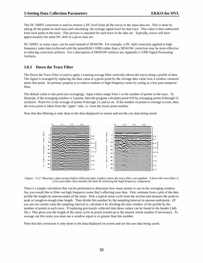
3.8.3 Down the Trace Filter
The Down the Trace Filter is used to apply a running average filter vertically (down the trace) along a profile of data. The signal is averaged by replacing the data value at a given point by the average data value over a window centered about that point. Its primary purpose is to reduce random or high frequency noise by acting as a low pass temporal filter.
The default value is one point (no averaging). Input values range from 1 to the number of points in the trace. To illustrate, if the averaging window is 5 points, then the program calculates point #10 by averaging points 8 through 12 inclusive. Point #11 is the average of points 9 through 13, and so on. If the number of points to average is even, then the extra point is taken from the ‘upper’ side, i.e. from the lower point number.
Note that this filtering is only done to the data displayed on screen and not the raw data being saved.
Figure: 3-12 Showing a data section before (left) and after (right) a down the trace filter was applied. A down the trace filter is a low pass filter that smooths the data by removing the high frequency component.
There’s a simple calculation that can be performed to determine how many points to use in the averaging window. Say you would like to filter out high frequency noise that’s affecting your data. First, estimate from a plot of the data profile the length (in nanoseconds) of the noise. Pick a typical noise cycle from the section and measure the peak-to-peak or trough-to-trough time length. Then divide this number by the sampling interval in nanoseconds/point. (If you are not certain what the sampling interval is, calculate it by dividing the time window of the profile by the number of points in each trace. If replaying previously collected data these values can be found in the header (.hd) file.) This gives you the length of the noise cycle in points (round up to the nearest whole number if necessary). To average out this noise you must use a window equal to or greater than this number.
Note that this correction is only done to the data displayed on screen and not the raw data being saved.
32

EKKO-for-DVL 3-Setting Data Collection Parameters
3.8.4 Background Subtract Filter
In some GPR applications, it is desirable to remove the transmit pulse and any other time invariant background signal. This can be achieved by using a running average filter which finds the average trace which is being observed and then subtracts it from the current data incoming from the system. This type of filter is useful if the targets are pipes and cables in a fairly flat-lying stratigraphy. Turning this filter on will subtract out the fairly flat-lying (or constant) events (like stratigraphy) and only leave the residual events (like diffractions from pipes and cables).
Such a filter may not be desirable for geological mapping. If one is looking at slowly varying stratigraphic horizons then this type of filter will remove these kinds of features from the data.
Note that this filtering is only done to the data displayed on screen and not the raw data being saved.
The basic equations describing what is going on are as follows. Each incoming radar trace is accumulated in the running average using an exponentially weighted past history. The mechanics are as expressed below.
Oi-incoming measured trace = 1, NptsAi=(b)Ai+(1-b)Oiis the running history average trace = 1, Npts
where N trace is the 1/e length of the running historyRi=Oi-Ai - residual trace after averaging background is removed
Generally, the selection of the number of traces to average over is dependent on the application and speed of data acquisition, etc. One should look at the data being acquired and look at the width of the localized features which one wants to see versus the rate of change of the "constant" background signals. One then picks the number of traces to be about the number which adequately spans the local features but still gives a reasonable average of the background.
Figure: 3-13 Showing a data section before (left) and after (right) background subtraction. This process is effective for emphasizing dipping reflectors like the responses from point targets like pipes.
For example, a pipe or cable anomaly may extend over to five or ten traces. One would then pick the number of traces to average over on the order of 20 to 40 traces. The length which one would actually use would depend on whether or not the average background, flat-lying events were slowly varying on this scale.
b e1
Ntrace------------------
=
33

3-Setting Data Collection Parameters EKKO-for-DVL
3.8.5 Optimize Color Plot
When data are plotted on screen in COLOR traces it sometimes appears “blocky”, especially when using a trace width of 4 or 8 pixels. This occurs because the colors applied to the amplitude values of a trace are repeated same 2, 4 or 8 times and this produces little squares of colors when viewed on the screen.
When this parameter is ON the colors between traces are interpolated or smoothed to eliminate the “blocky” effect. Thus, for example, rather than go from a black color on one trace to a white color on the adjacent trace, this option will fill in shades of grey in between so the data appears smoother and more continuous.
This process has no effect on the data being collected. It is only used to improve the screen display of the data.
Note that this process takes additional CPU time and if used during data collection, will slow down productivity. As such it will normally be OFF during data collection.
It can be used during data collection if the screen data display is important. However, it is probably most effectively used after data collection when the data are being replayed (see Section 4.3 on page 46).
3.9 System
Under SYSTEM are collected various user-programmable radar operating parameters.
3.9.1 Antenna Frequency
The first parameter to choose is the antenna frequency for the survey (see discussion in Section 3.1.5 on page 15). The following submenu will be displayed:
____________ System→Ant. Frequency________________________________________________________
Antenna Frequency (MHz): 12.5 25 50 (100) 200 Other
______Sensors & Software_______________________pulseEKKO 100 RUN____________________V 1.2_____
This menu is for entering the frequency of the antennas being used. The user has a choice of two methods of entering the antenna frequency. The easiest way is to choose one of the five frequencies shown: 12.5, 25, 50, 100 or 200 MHz. Alternatively, the user can select Other and manually enter the frequency. This method of entering the frequency is useful if the user is using a set of non-standard antennas.
It is important that the correct frequency be entered since this value is used in many computations including pulse width used in the DEWOW correction and for setting a default sampling interval (see below).
Note that the hardware cannot determine which antenna is attached. The user must correctly enter this parameter.
After the frequency has been selected the following screen is displayed:
____________ System_________________________________________________________________________
Frequency : 100 Time Window : 300 No. Stacks : 64Points : 375 Return Sampling Int : 800
______Sensors & Software________________________pulseEKKO 100 RUN___________________V 1.2_____
34

EKKO-for-DVL 3-Setting Data Collection Parameters
The Frequency and Points fields are informational and are not directly accessible. The Frequency label lists the frequency selected in the previous menu. Points are calculated based on the time window length and the sampling interval. For example, using the parameters listed above, the number of points is calculated as follows:
points = time window/sampling interval
= 300 ns / 800 ps
= 300 ns / 0.8 ns
= 375
The number of points is important because pulseEKKO systems have limits on the number of points that can be collected. On older systems this limit is 2560 while newer systems have a limit of 5000 points. If these limits are exceeded, an error message will be displayed suggesting that the time window be shortened and/or the sampling interval increased to reduce the number of points into the acceptable range.
3.9.2 Time Window
The Time Window setting determines how long (and therefore how deep) the radar system will probe the subsurface. It is important that it be set to a value appropriate for the depth of the survey target (see Section 3.1.6 on page 15).
When Time Window is selected from the menu a new menu appears:
____________ System_________________________________________________________________________
Time Window (ns) : 300
Window Range (m) : 15.0
Return
Warning: Depth assumes full time window and a velocity of: 0.1
______Sensors & Software_______________________pulseEKKO 100 RUN___________________V 1.2______
With older pulseEKKO systems the Time Window is selectable over the range from 50 to 2000 nanoseconds in any steps. Newer systems have time windows from 1 to 32767 nanoseconds.
It is also possible to input a depth in metres into the Window Range field and have the program automatically calculate an appropriate time window. The depth assumes the velocity set under the Velocity menu (See Section 3.10 on page 36).
3.9.3 Sampling Interval
Sampling Interval is an important parameter to be set correctly (see the discussion in Section 3.1.7 on page 16). On older systems, the sampling interval is user selectable over the range from 800 to 8000 picoseconds in steps of 800 ps. With newer systems the sampling interval is 10 to 20000 ps in steps of 2 ps.
35

3-Setting Data Collection Parameters EKKO-for-DVL
Based on the frequency selected, an appropriate sampling interval is automatically input into the field. As well, the upper part of the screen displays a table listing good sampling intervals for each frequency. This is similar to the one in Section 3.1.7 on page 16. The sampling interval automatically input is usually the sampling interval listed on the table.
It is important not to choose a sampling interval that is too large for the particular antenna frequency, otherwise the data may be aliased. Choosing a sampling interval too small will increase the data volume and slow down the data collection process.
3.9.4 No. Stacks
Stacking can improve data quality but can also slow data production (see the discussion in Section 3.1.8 on page 16 for selecting an appropriate number of stacks). This menu allows the user to select the number of stacks to use when collecting data.
When Number of Stacks is selected, the following display will be seen:
__________________System→No. Stacks________________________________________________________
A : 1 B : 2 C : 4 D : 8 E : 16
F : 32 G : 64 H : 128 I : 256 J : 512
K : 1024 L : 2048
______Sensors & Software_______________________pulseEKKO 100 RUN___________________V 1.2______
The user selects the number of stacks by entering one of the letters above, by highlighting the desired number and pressing <Enter>. For example, selecting E means 16 full data traces are acquired and averaged to create the data trace displayed and stored to disk. Generally, selecting 4 to 64 stacks is sufficient.
3.9.5 Return
The Return option returns the user to the main RUN menu.
3.10 Velocity
If a depth axis on the real-time display is desired, or the user wishes to get the time window by entering depth rather than time the user should supply the program with the average radar wave propagation velocity (in m/ns). When this option is selected, a table of velocities for a number of common geological media is displayed to serve as a guide. A velocity of 0.1 m/s is a good average to use when unsure about the material being produced. Simply enter the velocity and press <Enter>.
36
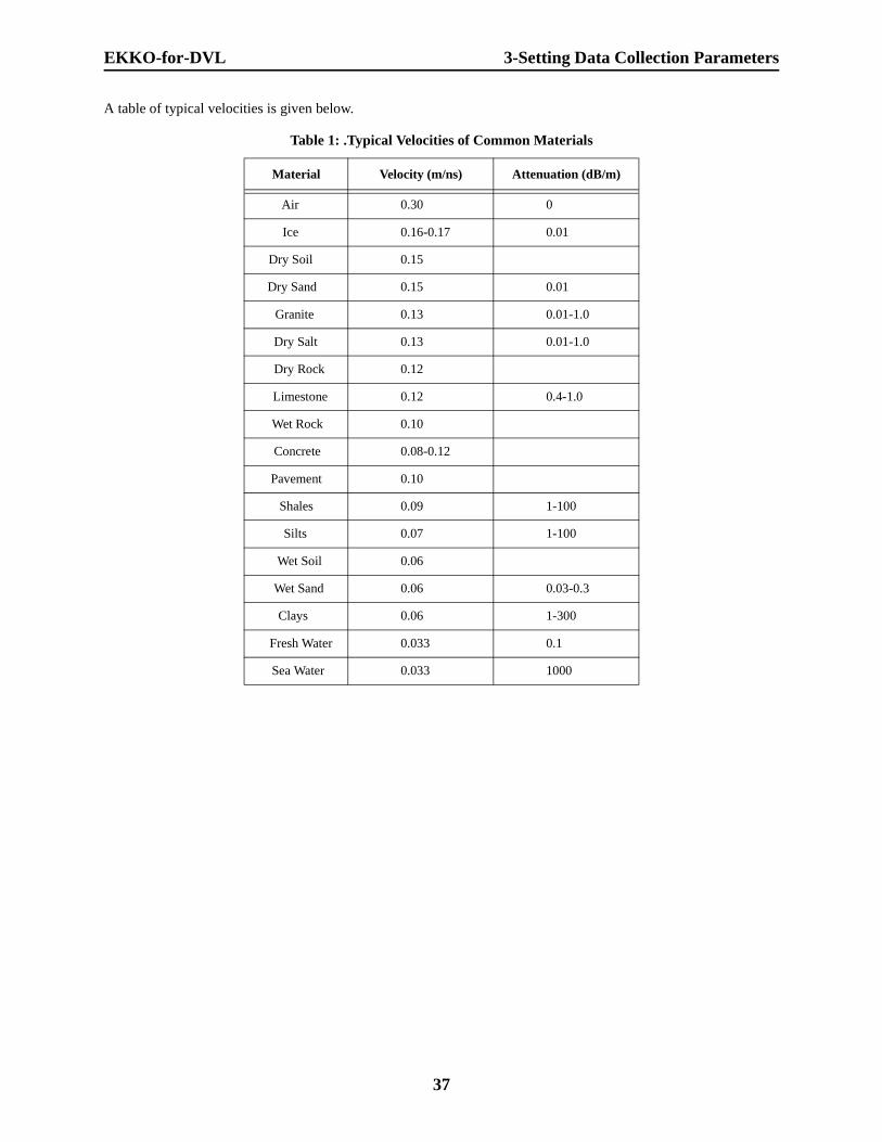
EKKO-for-DVL 3-Setting Data Collection Parameters
A table of typical velocities is given below.
Table 1: .Typical Velocities of Common Materials
Material Velocity (m/ns) Attenuation (dB/m)
Air 0.30 0
Ice 0.16-0.17 0.01
Dry Soil 0.15
Dry Sand 0.15 0.01
Granite 0.13 0.01-1.0
Dry Salt 0.13 0.01-1.0
Dry Rock 0.12
Limestone 0.12 0.4-1.0
Wet Rock 0.10
Concrete 0.08-0.12
Pavement 0.10
Shales 0.09 1-100
Silts 0.07 1-100
Wet Soil 0.06
Wet Sand 0.06 0.03-0.3
Clays 0.06 1-300
Fresh Water 0.033 0.1
Sea Water 0.033 1000
37

4-Data Collection EKKO-for-DVL
4 Data CollectionWhen all necessary parameters have been entered and all options chosen, selecting Run will initiate data collection.
There are three different RUN modes: Graph, Collect and Replay.
____________ Run________________________________________________________________________
Graph Collect Replay
_______Sensors & Software________________________pulseEKKO 100 RUN_________________V 1.2______
Graph mode is used to make sure that all wiring and connections are correct, all parameters are properly set and that valid data are being collected. GRAPH mode displays the radar trace in the traditional oscilloscope scan format (see Figure 4-1). The GRAPH mode should normally be run first, prior to data collection and storage. Data cannot be saved in GRAPH mode. Once the user is satisfied that everything is working, they can switch to COLLECT mode to begin data collection.
Collect mode is selected when the user is ready to collect data.
Replay mode is used to plot any previously collected data to the screen. This makes it possible to quickly review the data and perhaps try to enhance it using different gains or filters.
4.1 GraphThe Graph mode serves two main functions:
a) to ensure that valid data are being collected properly, and
b) to set the location of the transmit pulse (which is the reference timezero or the first break).
4.1.1 Graph Screen
A sample of a screen data plot while in Graph mode is shown in Figure 4-1. Note that in this plot the time axis is in the horizontal direction and the radar amplitude (in millivolts) is in the vertical direction. Below the plot, the trace number, time window, sampling interval, number of points and stacks are listed.
Data collection can be paused and a menu displayed by pressing the button under PAUSE.
Figure: 4-1 A sample of a screen data plot while using Graph mode. The parameters below the graph, the trace number, time window, sampling interval, points and stacks are listed and are fairly straightforward to understand. The other parameters listed
are explained below
38

EKKO-for-DVL 4-Data Collection
When running in GRAPH mode the user may remove the grid and the shaded region for cosmetic purposes by pressing the GRID button.
The user can toggle the correction (see Section 3.8.2 on page 30) from DEWOW to DC Shift to None by pressing the CORRECTION button.
The other parameters listed on the screen in Graph mode are explained below.
Timezero Adjust is the value used to adjust the first break to the ideal region. The value has no impor-tance to the radar data; it is only used for the adjustment of the initial radar pulse to the desired position within the time window.
Input indicates the port that the data are being collected through. If the High Speed option is ON then data are collected from the parallel port. If the High Speed option is OFF then data are collected through the serial port.
Voltage measures the battery voltage of the battery supplying power to the console. If this value drops below 10.5 or exceeds 15.0 volts the survey should be discontinued and the battery recharged or replaced.
The value immediately to the right of the voltage value is the trigger value. It will change as the external trigger or odometer is pressed.
Fid # means the fiducial number and only occurs if the system is in Continuous mode. If the trigger is pressed while in Continuous mode, a fiducial mark is written to the com-ment field of the trace being collected. This value increments as the trigger is pressed and lets the user know the number of the last fiducial mark written.
4.1.2 Error Messages
If the radar is not connected properly, an error message will be displayed indicating the possible cause of the problem. Section 4.4 on page 47 discusses the meaning of these messages and how to remedy the problem.
4.1.3 Timezero Adjustment
Assuming that data are coming in, the first thing that must be done is to ensure ‘timezero’ is in the correct location. Timezero, for our purposes, is defined as the first arrival of the radar wave; it is used as a convenient reference starting point for the trace, hence the name: timezero.
Timezero should be located within the shaded portion on the screen (see Figure 4-1). Locating timezero to the right (further in time) of the shaded portion has no ill effect on the program, it just means possible reflectors may be lost off the bottom of your recording window. Locating timezero to the left of the shaded region should be avoided. The AGC and SEC gain function can be set up in the data plotting programs to use the data before timezero to calculate average background noise.
The location of timezero is affected by a number of factors. These factors include, various system hardware components, length of fiber optic cables, separation of transmitter and receiver antennas, and the total time window (shaded area is roughly 10-15% of the total time window).
39

4-Data Collection EKKO-for-DVL
4.1.4 Data Collection Modes
If the Field Line parameter Operating Mode (see Section 3.4.2 on page 19) is set to ‘CONT’ (i.e. CONTinuous) or FREE (i.e. Free-running), the radar will continuously collect new data and plot it on the screen. If Operating Mode is set to ‘STEP’, the user must press the B button, the trigger or use the odometer to collect another trace.
The system is ready to collect the next trace when the “Hit Trigger” sign appears in the bottom right part of the screen.
4.1.5 Graph Data Menu
Pressing the PAUSE button while running in graph mode brings up menu items which will be displayed at the bottom of the screen. These are:
Continue
Go back to Graph mode data collection.
Find T0
Adjust ‘timezero’ location. To set 'timezero', the transmit and receive antennas should be placed close to one another. This assures a large first arrival with minimal propagation delay. The shaded band representing the ‘ideal’ location is displayed on the screen (see Figure 4-1). The purpose is to adjust the ‘timezero’ location so that it falls within that shaded band. There are 4 options for adjusting timezero: Arrow Adjust, Automatic, Manual and Full Search.
Arrow Adjust is used if the transmit pulse is visible on the screen but needs to be moved into the shaded region. After pressing Arrow Adjust, the left and right arrow keys can be used to move the pulse into the shaded region. When the pulse is in the proper position ENTER is pressed.
Pressing Automatic initiates an automatic search and timezero adjust to bring the timezero location within the shaded ‘ideal’ region. The automatic search and adjust, while not perfect, should work most of the time. It works on the assumption that the first break (first signal to arrive) is strong compared to the surrounding background noise. If antennas are at a large separation or there is a large amount of external noise then this automatic adjustment may not function correctly.
For Manual adjustment of timezero a value in nanoseconds is entered. A higher value will shift the trace to the right (later in time), while a lower value will shift it to the left (earlier in time). The absolute numbers have no meaning and are dependent on factory adjustments of the hardware and cabling characteristics. To see the effect of an adjustment, the user must press CONTINUE to collect and display a new data trace.
If timezero has not been found, conduct a Full Search. All possible positions of the transmit pulse are searched in succession. When the pulse appears on the screen near the shaded region, the user must press a button to stop it and then use the left and right arrow keys to move it into the shaded region.
If no transmit pulse is found there is a problem with the transmitter; see Transmitter Problems: No Signal on Screen in Section 5.4 on page 52.
Mode
This item allows the user to change the operating mode of the system to Continuous/Free-running or Step (See Section 3.1.2 on page 13 (Operating Mode) and Section 3.4.2 on page 19 (Fieldline - Mode)).
When Continuous/Free-running mode is selected it allows the user to change the Move Delay time between collecting two successive traces. Move delay determines the number of seconds that the program will wait in between data collection. This delay time allows the operator to move the antennas to the next profile position.
40

EKKO-for-DVL 4-Data Collection
The user is the best judge of what this delay time should be, depending on such factors as the radar site, operator experience, weather, etc. The amount of delay between traces is affected by the number of points in the trace and the speed of the computer being used. Therefore, trial and error must be used to find the appropriate setting.
Note that Move Delay only makes sense when the Operating Mode is ‘CONT’ (i.e. CONTinuous or FREE). In ‘STEP’ mode, the user decides when to collect the next trace by pressing the B button, trigger or using the odometer.
Scale
This will allow the user to modify the maximum amplitude displayed on the graph scale. This parameter may take on any value between 1 and 50 millivolts. The default value is 50.
Quit
This button is used to get out of the run mode and return to the main RUN menu.
Exiting Graph: The user will normally need to use FIND T0 button to adjust the timezero location so that it falls within the recommended region. Once the user is happy that everything is working properly and all parameters are correctly set, pressing the QUIT button exits GRAPH mode and returns the user to the main menu. At this point, the user can select RUN - COLLECT to begin data collection.
4.2 Collect
As the name implies, COLLECT mode is selected when the user is ready to collect data. The following screen will be seen:
_________Run_____________________________________________________________________________
Do Not Save Data Input File Name Replay
_______Sensors & Software______________________pulseEKKO 100 RUN__________________V 1.2_______
4.2.1 Do Not Save Data
The first selection means data are collected but not saved to disk. This option can be selected if the user just wants to see the data plotted in stacked profile fashion (see Figure 4-2) and does not want to save the data to a disk file.
4.2.2 Input File Name
The directory and file name are listed on this screen. The directory the data is saved to is that name specified under Job - Set Directory (see Section 3.6.1 on page 27).
The data file name will automatically be filled in. File names always have the prefix LINE followed by a 4 digit number. The user change the number portion of the file name using the number buttons. When a series of data files are collected the file name will automatically default to the next available number, i.e. LINE0000, LINE0001, LINE0002 etc.
For user reference, pressing the A button will list all the names of the GPR data files currently saved in the directory.
4.2.3 Data Collection
Once the file name or Do Not Save Data is selected, the program begins data collection.
41
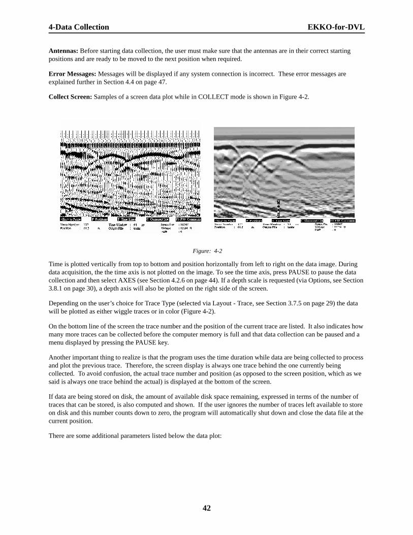
4-Data Collection EKKO-for-DVL
Antennas: Before starting data collection, the user must make sure that the antennas are in their correct starting positions and are ready to be moved to the next position when required.
Error Messages: Messages will be displayed if any system connection is incorrect. These error messages are explained further in Section 4.4 on page 47.
Collect Screen: Samples of a screen data plot while in COLLECT mode is shown in Figure 4-2.
Figure: 4-2
Time is plotted vertically from top to bottom and position horizontally from left to right on the data image. During data acquisition, the the time axis is not plotted on the image. To see the time axis, press PAUSE to pause the data collection and then select AXES (see Section 4.2.6 on page 44). If a depth scale is requested (via Options, see Section 3.8.1 on page 30), a depth axis will also be plotted on the right side of the screen.
Depending on the user’s choice for Trace Type (selected via Layout - Trace, see Section 3.7.5 on page 29) the data will be plotted as either wiggle traces or in color (Figure 4-2).
On the bottom line of the screen the trace number and the position of the current trace are listed. It also indicates how many more traces can be collected before the computer memory is full and that data collection can be paused and a menu displayed by pressing the PAUSE key.
Another important thing to realize is that the program uses the time duration while data are being collected to process and plot the previous trace. Therefore, the screen display is always one trace behind the one currently being collected. To avoid confusion, the actual trace number and position (as opposed to the screen position, which as we said is always one trace behind the actual) is displayed at the bottom of the screen.
If data are being stored on disk, the amount of available disk space remaining, expressed in terms of the number of traces that can be stored, is also computed and shown. If the user ignores the number of traces left available to store on disk and this number counts down to zero, the program will automatically shut down and close the data file at the current position.
There are some additional parameters listed below the data plot:
42

EKKO-for-DVL 4-Data Collection
‘Voltage’ measures the battery voltage of the battery supplying power to the console. If this voltage drops below 10.2 volts the computer will beep and a warning will appear on screen. Depending on the temperature and other conditions the system can continue to run to about 9.8 volts but it is best to finish the survey line and recharge or replace the battery as soon as possible. It is also a good idea to discontinue the survey if battery voltage exceeds 15.0 volts.
The value immediately to the right of the voltage value is the trigger value. It will change as the external trigger or odometer is pressed.
‘Fid #’ means the fiducial number and only occurs if the system is in Continuous mode. If the trigger is pressed while in Continuous mode, a fiducial mark is written to the comment field of the trace being collected. This value increments as the trigger is pressed and lets the user know the number of the last fiducial mark written.
Pressing the POSITION button will toggle positions values written vertically on the traces. This allows the user to see the position of features in the data without having to pause data collection.
Pressing the TIMELINE button will toggle timing lines being plotted horizontally across the traces.
The user can toggle the correction (see Section 3.8.2 on page 30) from DEWOW to DC Shift to None by pressing the CORRECTION button.
4.2.4 Data Collection Sequence
If the Operating Mode (see Section 3.4.2 on page 19) is set to ‘CONT’ (i.e. CONTinuous) or ‘FREE' (i.e. FREE-running), the radar will go through the following cycle:
a) wait the desired number of seconds specified by the Start Delay (see Section 3.4.9 on page 20),
b) start a beeping tone,
c) collect one trace,
d) stop the beep,
e) wait for the specified number of seconds in Move Delay (see Section 3.4.10 on page 20),
f) check to see if data collection should pause (see Pause Trace in Section 3.4.6 on page 20), and
g) then back to a) to repeat the cycle.
On the other hand, in ‘STEP’ mode, the following cycle is followed:
a) wait the desired number of seconds specified by the Start Delay (see Section 3.4.9 on page 20),
b) start a beeping tone,
c) collect one trace,
d) stop the beep,
e) display READY indicator,
f) wait for user to hit the B button, trigger or the odometer to move one StepSize (see Section 3.4.8 on
43

4-Data Collection EKKO-for-DVL
page 20), and
g) then back to b).
Normally the antennas should not move while data are being collected, as indicated by the time duration that the beeping tone is on. Keeping the antennas static assures the highest quality stacked data. When the beep stops, the antennas should be moved to their next position in preparation for the next trace. Obviously holding antennas stationary is impractical when a continuous moving platform is used for data acquisition.
4.2.5 Odometer Data Acquisition
Step mode data acquisition can also be controlled by an odometer triggering the radar system to collect data at specified position increments. In this operating mode, it is possible to move too fast and trigger too quickly for the system to keep up.
When using the odometer, the software can detect when the odometer is triggering the system too quickly and will cause the computer to beep and write a warning to the screen. When this occurs position accuracy is retained but some traces may be skipped and “gaps” will appear in the data when it is plotted. Use the FILLGAP function (in EKKO_EDIT or Win_EKKO) to interpolate traces into any “gaps” in the data set.
4.2.6 Collect Data Menu
Pressing the PAUSE button suspends the data collection cycle and displays a menu that is displayed at the bottom of the screen. The menu items are:
Continue
Go back to COLLECT mode and continue with data collection.
Axes
Pressing AXES will toggle the time and depth axes being written to the screen. Note that in order to see the depth axis, the Option - Depth Axis parameter must have been set to ON (see Section 3.8.1 on page 30).
Air Velocity Grid
A feature that can often be seen in the data during data acquisition is a reflection that looks like a hyperbola or inverted ‘U’. This is a common response from point targets like buried pipes. This phenomenon occurs because radar energy does not radiate as a pencil-thin beam but more like a 3D cone. Therefore, reflections can appear on the record even though they are not directly below the radar system. Thus, the radar system “sees” the pipe before and after going over top of it and forms a hyperbolic reflection.
However, hyperbolic reflections can also be caused by objects not in the subsurface such as fences, overhead wires and, in some conditions, even large trees.
An important part of data interpretation is learning to recognize these unwanted “air” events and differentiate them from the wanted subsurface events. Good field notes are indispensable for helping identify unwanted events on the data.
One way of doing this is to use the “tails” of the hyperbola to measure the radar velocity to the object that caused that hyperbola. Obviously, if the object is in air, the radar velocity (v = 0.3 m/ns) will be much faster than if it is in the ground (v ~ 0.1 m/ns).
44

EKKO-for-DVL 4-Data Collection
To assist in this determination, the RUN program will plot an air velocity grid to the screen the AIRGRD button is pressed (Figure 4-3). This allows the user to quickly see if a hyperbolic event is a surface feature by seeing if the tails of the hyperbola are parallel to the grid lines.
Figure: 4-3 Ground Velocity Grid
Similar to the air velocity grid described above, the RUN program will also plot a ground velocity grid to the screen if the GRNDGRD button is pressed. The velocity used is set in the Velocity parameter (see Section 3.10 on page 36). Thus, if a hyperbolic event is a subsurface reflection from a point target, the radar velocity to that target can be quickly estimated. Once the velocity is estimated it can be used to plot a depth axis with a fair degree accuracy.
Note these velocity grids are meaningless if positioning is not accurate or the system is running in 'FREE-RUN' mode.
Note that these velocity grids cannot be erased from the screen but will eventually scroll off.
Mode
This item allows the user to change the operating mode of the system to Continuous/Free-running or Step (See Section 3.1.2 on page 13 - Operating Mode and Section 3.4.2 on page 19 - Fieldline - Mode).
Also, when Continuous/Free-running mode is selected it allows the user to change the Move Delay time between collecting two successive traces. Move delay determines the number of seconds that the program will wait in between data collection. This delay time allows the operator to move the antennas to the next profile position.
The user is the best judge of what this delay time should be, depending on such factors as the radar site, operator experience, weather, etc. The amount of delay between traces is affected by the number of points in the trace and the speed of the computer being used. Therefore, trial and error must be used to find the appropriate setting.
Note that Move Delay only makes sense when the Operating Mode is ‘CONT’ (i.e. CONTinuous). In ‘STEP’ mode, the user decides when to collect the next trace by pressing B button, trigger or using the odometer.
45

4-Data Collection EKKO-for-DVL
Gains
This function key serves the same purpose as the Gains option in the main RUN menu, namely to select the type of gain function and their parameters. It is included here for convenience since it is often difficult to decide on the gain function and/or parameters beforehand without having a good look at the data. This function key allows the user to adjust the gain in real-time without having to exit back to the main RUN menu. The new gain is only applied to subsequent traces; traces already collected are not replotted. These gains are only applied to the data being displayed, all data stored is in the raw format.
Once inside this routine, the buttons are assigned as follows: AGC, SEC, CONST, NONE, AUTO. The parameters needed in AGC, SEC, USER and CONST are already explained in Section 3.5 on page 20.
Filters
Pressing the FILTERS button allows the user to apply real-time filtering to the data being collected. These filters can also be set up in the Main RUN menu, but having the option here allows these filters to be changed without leaving the data collection process. Keep in mind that this filtering is only applied the displayed data, not the data being saved; the saved data are always stored in raw format. The 2 filters that can be applied are a Down the Trace filter and a Background Subtraction filter. For details on these filters, see Section 3.8 on page 30.
Quit
This function key is used to get out of the run mode and return to the main RUN menu. In addition, if data are being stored to disk during COLLECT mode, this function key takes care of the details of updating and closing all files.
It is very important therefore that the user exits properly by using the QUIT key rather than by simply turning off the DVL.
4.3 Replay
After GPR data files have been collected, it is possible to view them using the Replay option under the Run menu item.
When Replay is selected, the user must then input the name of an existing file to plot. This is done exactly the same as selecting a file name for data collection (see Section 4.2.2 on page 41) except that in this case the file name must already exist. For user reference, pressing the A button will list all the names of the GPR data files currently saved in the directory.
Only files in the current directory can be selected. To see files in a different directory, change the directory under Set Directory (see Section 3.6.1 on page 27).
Replaying data can be very useful because it allows the user to quickly modify the plot with different gains (see Section 3.5 on page 20), filters (see Section 3.8.3 on page 32 and Section 3.8.4 on page 33) and color palettes (see 3.7.5 on page 29) to try and enhance the feature of interest. Data can also be plotted with the velocity grids 4.2.6 on page 44) to determine the velocity in the material being scanned or check for airwave reflectors.
Each time the CONTINUE button is pressed the data is replotted so if settings are changed, the modified image replaces the old one.
46

EKKO-for-DVL 4-Data Collection
4.4 Error Messages
In the course of running this program, various error messages may be encountered. Simple errors in data entry are followed by an error message, usually on the second to last line of the screen. These messages are self-explanatory; the remedy is usually to correct the entry in question. Errors that occur during data collection are more serious and will be discussed here.
The errors that occur during data collection can be categorized into three types:
a) Radar system errors,
b) File related errors, and
4.4.1 Radar System Errors
There are two radar system error messages one may encounter:
a) Console related
b) Receiver related
Console Related Errors
Console related errors are generated whenever the computer fails to communicate with the console for any reason.
These errors are indicated by one of the following messages:
CONSOLE ERROR #n
CONSOLE ERROR #n. CHECK CONNECTIONS (1) Retry or (2) Quit
RETRY ERROR #1. CHECK CONNECTIONS (1) Retry or (2) Quit
The first of these messages may be encountered as soon as the Run option of the main RUN menu is chosen. This message is accompanied by a list of things to do to try and solve the problem (shown below). The message appears until a key is hit after which the program returns to the main RUN menu.
The other error messages are generated if the program is already in the process of data collection. The user is given an opportunity to correct the problem and press the 1 button to continue.
The most common causes of these types of errors are the following:
a) Console-to-DVL connection is loose or faulty.
b) Console power source is low or dead. It should be at least 10.5 V and preferably 12V
c) The fuse connected to the console power source input has blown. If this occurs the red light above the POWER receptacle on the console will not be lit.
d) The fuse connected to the RS232 serial line has blown. Remove the fuse, situated above the RS232 receptacle on the console and replace.
e) Console to DVL connection was made after the console or DVL were turned on. Disconnect console power and reconnect.
47

4-Data Collection EKKO-for-DVL
f) The serial port connected to the radar system is different than that under Layout - Port (see Section 3.7.3 on page 28).
If all 6 things above are alright, then refer to Section 5 on page 49 - Troubleshooting for a more exhaustive check list.
Receiver Related Errors
Receiver related errors are indicated by the following message:
RECEIVER NOT TURNED ON. (1) Retry or (2) Quit
RECEIVER ERROR 5 (1) Retry or (2) Quit
RECEIVER ERROR 6b (1) Retry or (2) Quit
If this error is encountered, check that the receiver is turned on, that the batteries for the receiver are properly charged and that the receiver-to-console fiber optic cable is not damaged and properly connected. Again, Section 5 on page 49 contains more exhaustive tests if the problem is not obvious.
Transmitter problems are dealt with in Section 5 on page 49 - Troubleshooting. The most common symptom is a trace with no signal. Please refer to the Troubleshooting section if you think you have a transmitter problem.
4.4.2 File Related Errors
If the path\filename supplied by the user for storing the data already exists, then the following message appears:
FILE ALREADY EXISTS !
Over Write ? (1) Yes (2) No
Answering Yes by pressing the 1 button will cause the existing file to be overwritten and the original data will be permanently lost. Pressing the 2 button for No returns the user to the main RUN menu so that a new path\filename can be entered.
As the data are stored on disk, if the program finds that there is no more room on the disk, it prints the following message:
OUT OF DISK SPACE ! CLOSING THIS FILE...
The program will close the current file, update the header file and exit the COLLECT mode.
If the computer encounters a disk error while writing the data to disk the following message is displayed:
Data Write Error! Any Button To Exit...
Finally, one may encounter one of the following error messages:
ERROR WHILE OPENING HEADER FILE
ERROR WHILE UPDATING HEADER FILE
ERROR WHILE RE-OPENING DATA FILE
These messages should be very rare and may indicate a disk drive failure. They are non-recoverable errors; the program returns to the main RUN menu.
48
EKKO-for-DVL 5-Troubleshooting
5 Troubleshooting Earlier sections (see in particular Section 4.4 on page 47) have discussed a number of error conditions and their remedies. In this section, a more thorough discussion of the error conditions will be presented together with a systematic step-by-step procedure for tracking down the source of the problem.
5.1 System Console Error
In Section 4.4.1 on page 47 we encountered what we called Radar System Errors, one of which is indicated by the error message:
CONSOLE ERROR #1 CHECK CONNECTIONS (1) Retry or (2) Quit
This problem indicates that the communications between the console and the computer is faulty, the console battery is not charged or the console is damaged.
The following checks should be carried out.
a) With the system completely hooked up turn the console OFF then back ON again (usually by discon-necting the power cable momentarily). Retry system.
b) Check if the console power source is at least 10.5 volts (12 volts is better) and that the connections to the console are in good condition. Ensure the red light on the front panel of the console is ON.
c) Check the 2A fuse above the Power connection on the console and ascertain if the 12V source is connected with the correct polarity. The red light is located AFTER the fuse. If the red light is off and the fuse is OK, the problem lies in either the power cable or battery.
d) Check that the RS232 cable is securely plugged in. Also check that no damage has occurred to the RS232 cable. If unsure, the RS232 cable can be tested using an ohm-meter. This involves testing the internal cable connections along its length. If the cable is OK all the following tests will have a resistance of zero. A broken cable is indicated if any of the tests have an infinite resistance.
The serial port connection end of the cable is a socket D-9 connector. If you look closely these are numbered 1 to 9. (See Figure 5-1).
The other end of the cable is the console lemo connection end. Hold this end of the cable so that the 2 male pins are at the bottom as you look at it and the one female socket is at the top. With this orientation the pin layout is:
1) serial port D-9 connector female socket #2 to bottom right pin.
2) serial port D-9 connector female socket #3 to bottom left pin.
3) serial port D-9 connector female socket #5 to top female socket.
49

5-Troubleshooting EKKO-for-DVL
Figure: 5-1
e) Check the 2A fuse located above the RS232 (computer to console) cable connection on the console.
f) Make sure that the serial port setting in Layout - Port (see Section 3.7.3 on page 28) is set to the correct port (COM1).
g) Very rarely it is possible that your DVL cannot transfer data to the radar system at 19200 baud. Reduce the baud rate to 9600 or lower (see Section 3.7.1 on page 28), reset the console by interrupting the power supply briefly and retry running the system.
h) If you are still having problems running the radar system, the problem is either with the console itself or the DVL. The console or DVL may need factory service.
5.2 DVL Problems
If, when trying to run the radar system, you are getting a consistent console error and none of the suggestions under System Console Errors have worked, the problem may be DVL related. Also, it is probably a DVL problem if the pulseEKKO RUN software always returns to the Main Menu without running the system or “hangs” the DVL and forces the user to have to reboot.
5.3 Receiver Error
If any of the following errors occur on the screen:
Receiver Not turned On!! (1) Retry or (2) Quit
RECEIVER ERROR 5 (1) Retry or (2) Quit
RECEIVER ERROR 6b (1) Retry or (2) Quit
Always hit R to retry the system. The error message after a retry is very important for isolating where in the system the problem is occurring.
If the following error occurs after pressing Retry:
RETRY ERROR 1 (1) Retry or (2) Quit
the problem has to do with the console (see Section 5.1 on page 49).
50
EKKO-for-DVL 5-Troubleshooting
If, however, after pressing Retry you get a receiver error again then perform the following checks:
a) Check that the red POWER light on the top of the receiver is ON. If not, then press the ON/OFF switch once to see if the light comes ON. If it does, press the 1 (Retry) button to see if the radar system will run. If the red POWER light still does not light up or flashes, check to make sure the batteries are fully charged.
b) Check the condition of the fiber optic cables. Look for any sign of stress or damage. Replace, if possible.
c) While pressing the 1 (Retry) button see if the red RUN light on the top of the receiver flashes each time you press retry. This light may be difficult to see if you are collecting data at a low number of stacks or in bright sunlight. If you are not sure if the light is coming on, increase the number of stacks to 1024 and try this procedure again. If the RUN light is flashing go to step e).
d) If the RUN light is still not flashing when pressing 1 (Retry), try to determine if the failure is caused by the receiver, the console or the fiber optic cables, by the following procedure:
Set the system up with a time window of 1500 ns, stacks at 1024 and sampling interval at 800ps and try running the system in Graph mode. Unplug the grey receiver fiber optics at the console.
Continue to hit the 1 (Retry) button. A red light should be seen coming from the grey receiver hole in the console each time the retry is pushed. If this red light is not visible in the grey receiver socket the problem appears to be the console; see section “Checking the Console” below.
Plug the grey receiver fiber optic cable back into the console. Unplug the INPUT (black) fiber optic cable at the receiver. Look for the red light coming from the end of the cable (keep pressing the 1 (Retry) button). If this red light is not visible or very dim, the problem appears to be the fiber optic cable; replace it and try running the system again.
Plug the black (INPUT) fiber optic cable back into the receiver and unplug the grey receiver fiber optic cable at the console. Hold the end of the fiber optic cable to a light source. This can be a flashlight, sunlight or even the light coming from the red POWER light on the console or receiver. Check 2 things: 1) Watch to see if the red RUN light on the receiver comes on and 2) unplug the OUTPUT (grey) fiber optic cable on top of the receiver and see if there is a light visible down the grey socket. If no light appears in the grey socket then the problem appears to be with the receiver; see “Checking the Receiver” below.
e) Plug the grey receiver fiber optic cable back into the console and the OUPUT (grey) fiber optic cable back into the top of the receiver. Unplug the black receiver fiber optic cable from the console. While pressing the 1 (Retry) key look at the end of the cable to see if a red light is visible at the end of the cable. If this red light is not visible the problem appears to be the fiber optic cable; replace it try running the system again. If the system is still not running see “Checking the Console” below.
Checking the Console:Carefully remove the back of the console and check the short fiber optic cables inside. As a test, these short sections of cable may be bypassed by plugging the long fiber optic cable directly into the electronics. Replace or polish the short cables if needed.
Checking the Receiver:If the above process failed while checking the light in the receiver, open the battery cover on the side closest to the fiber optic cable connectors and remove the battery. Remove the screws holding the sheet metal plate and carefully pull the plate out far enough to reveal the short fiber optic cables inside the receiver. Check the short fiber optic cables inside. As a test, these short sections of cable may be bypassed by plugging the long fiber optic cable directly into the electronics. Replace or polish the short cables if needed.
If none of the above solutions solve the problem, contact Sensors & Software Inc.
51

5-Troubleshooting EKKO-for-DVL
5.4 Transmitter Problem: No Signal on Screen
a) In Graph mode try the Automatic timezero search. Keep the antennas about one antenna length apart.
b) If the error comes up “No Signal Found” then try using the Full Search option in Graph mode timezero search (see Section 4.1.5 on page 40) to look for the pulse.
If the pulse still cannot be found do the following checks:
Make sure the transmitter battery is properly charged and connected.
Check the condition of the single fiber optic cable to the transmitter, looking for any signs of stress or damage. Replace or repair if needed.
Check that the brass antenna sockets in the bottom of the transmitter and the brass antenna pins in the top of the antenna are properly tightened. Also check that there is a good contact between them.
Set the system up with a time window of 1500 ns, stacks at 1024 and sampling interval at 800ps. Unplug the grey transmitter fiber optics at the console.
With the system running, look for a red light coming from the grey hole in the console (single hole). Plug this cable back in and unplug the INPUT (black) cable at the transmitter. Check for a red light coming from the cable.
If the above process fails while checking the light in the cable then replace the cable.
If the above process fails while checking the light in the console, carefully remove the back from the console unit and check the short fiber optic cables inside the unit. As a test, these short sections of cable may be bypassed by plugging the long transmitter fiber optic cable directly into the electronics. Replace or polish the short cable if needed.
c) If the signal is still not found, set the system up with the maximum time window (2048 ns on older systems, 32000 ns on newer systems) and stacks at one. Run in Graph mode and use the Full Search option to look for signal. If the pulse is visible on the trace, adjust it to the shaded region. Now you should be able to change the time window back to the desired length and have timezero visible.
d) If the signal is still not found, contact Sensors & Software Inc.
5.5 Timezero Drifting
If the first break is drifting on the data set as shown below:
Figure: 5-2
52

EKKO-for-DVL 5-Troubleshooting
This is an indication that the system has not been given enough time to stabilize to its operating temperature. This effect is only severe when strong temperature contrast occur such as initially operating the unit outside in very hot or cold conditions after storage inside at “room” temperature. The drift is associated with the console electronics and keeping the console powered up at all times keeps the internal temperature stable. Allow 5 - 10 minutes to warm up before collecting data.
5.6 Timezero Jitter
If the first break is jumping up and down as shown below:
Figure: 5-3
This is an indication that the fiber optic cables are damaged. Check all cables and replace or repair. Check cables inside the units also (Transmitter, Receiver, and Console).
5.7 Battery Voltage Check
If battery power is a suspected cause of problems, always check the battery voltage with the battery under load. Checking a battery with no current drain will often give a false sense of the state of a battery. With the pulseEKKO system, the best way to check batteries is to connect the batteries to the unit that they supply, turn on the unit and measure the voltage.
5.8 Cannot Continue in Step Mode
In order to collect the next trace the B button, trigger or odometer must be pressed.
53

6-File Management EKKO-for-DVL
6 File ManagementGPR data files collected on a DVL can be transferred to an external computer or deleted from the DVL.
6.1 File Management Menus
From the main menu, pressing the 2 button selects File Management.
The first screen lists the names of the data directories on the DVL, i.e. STTE01, SITE02, SITE99 etc. Data directories are selected by highlighting the name using the arrow buttons and pressing the ENTER button.
When a directory is selected, the next screen shows the options available for working with that directory:
1 - Delete Directory2 - List Data Files3 - Select Another Directory4 - Export Files5 - Main Menu
Delete Directory will delete the directory and all the data files in the directory from the DVL. Before this is done the user has to verify that they want to deletion to be done.
List Data Files will list all the data files in the directory. It is in this menu that the user can decide to delete individual data files from the directory.
Selecting Another Directory takes the user back to the previous menu with the listing of all the data directories on the DVL.
Export Files is used to transfer data files to an external PC using the PXFER cable and the PXFER program. For more details see Section 6.2 on page 54.
6.2 Transferring Data Files to an External PC using the PXFER Program
Pressing the number 4 in the File Management menu transfers ALL the data files from the DVL to an external computer.
Note that it is not possible to use the PXFER cable to transfer data to computers running Windows NT or 2000.
To transfer all the data files in one directory from the DVL to an external computer, the computer must be connected to the DVL using the special parallel PXFER cable that is supplied with the system (see Section 6.2.1 on page 54). Note that this is a special cable and standard 25 pin to 25 pin or Laplink cables will not work. As well, the computer must have the utility program called PXFERxx.EXE running on it (Section 6.2.2 on page 55).
6.2.1 Connecting the Digital Video Logger to an External Computer
To transfer data from a DVL a cable called the parallel XFER (PXFER) cable is required. This cable is designed to connect the DVL to an external computer.
54

EKKO-for-DVL 6-File Management
Figure: 6-1 Parallel PXFER cable connections
The 2 connections that must be made before attempting to transfer data are:
1) Attach the 25 socket parallel connector to the 25 socket parallel port on back of the Digital Video Logger, and
2) Attach the 25 socket parallel connector the parallel port of the external computer.
WARNING: To avoid damaging any of the components, turn off the DVL and computer before making any of these connections.
6.2.2 Installing and Running the PXFER.EXE Program
The system should have come with a floppy disk containing the PXFERxx.EXE program, where xx is the version number, i.e. PXFER21.EXE is version 2.1.
To install the PXFERxx.EXE program, copy it from the floppy disk into a folder on the external computer. You may want to make a new folder for this program to reside in and also as a place to save data files. A suggested name for the folder is GPR_DATA.
Once the PXFERxx.EXE program has been installed on the computer and the user is ready to transfer data to the computer, the PXFERxx.EXE program needs to be run. This can be done using Windows Explorer or DOS.
To use Windows Explorer, find the PXFERxx.EXE program and double-click it.
To use DOS, open a DOS Window from Windows (Start - Program Files - DOS Prompt). Then change directories to the directory containing the PXFERxx.EXE program. For example, if this program was copied to the \GPR_DATA directory, type CD\GPR_DATA and press Enter. Then run the PXFERxx.EXE program by typing the name (without the extension) and pressing Enter, i.e. PXFER21.
When the PXFERxx.EXE program has been run, it will write the screen:
LISTEN MODE V2.1 USING PORT ADDRESS = 378
This means that it is ready to receive data transferred from the DVL to the LPT port number 1.
This command assumes that the data buffers are being transferred across Parallel Port 1 (LPT1). If using Parallel Port 2 (LPT2) or higher (LPT3, LPT4 etc.), specify the parallel port number after the PXFERxx program name. For example, for LPT2 use:
PXFERxx 2
55

6-File Management EKKO-for-DVL
6.2.3 Transferring Data Files
Once the parallel XFER cable is connected (Section 6.2.1 on page 54) and the PXFER software is installed and running (Section 6.2.2 on page 55), it is now possible to transfer all data buffer files to the external computer.
On the DVL, from the File Management menu, press number 4 - Export Files.
The data will be transferred from the DVL to the computer and saved in the current working directory. The progress of the data transfer will be displayed on the DVL screen and the external computer.
If errors occur during the data transfer it may be that Windows is interfering with the transfer of the data. If possible, it is best to transfer the data while in DOS mode on the external computer. To do this from WIN95 or 98, click the Start button and then select Shut Down and finally Restart the computer in MS-DOS mode. Then run the PXFERxx program and try the data transfer again.
Note that it is not possible to use the PXFER cable to transfer data buffers to computers running Windows NT or 2000.
When the data transfer is complete, press the ESC key on the external computer to exit from the PXFERxx.EXE program. Press any button on the DVL to return to the main menu.
Note that once the GPR data files have been transferred to the PC, they should be moved to another directory on the PC. This will allow more data files from another directory on the DVL to be transferred to the PC. Remember that since the data files are given set names like LINE0000, LINE0001 etc., existing data files in the directory on the PC will be overwritten by the new data files being transferred without warning.
6.2.4 Parallel Port not bi-directional Error
Sometimes, when attempting to transfer data to the PC, the error message "LPT1 is not bi-directional" may appear on the DVL screen. When transferring data from the DVL unit to a PC, the printer port is used. The PXFER.EXE program utilizes the functions of a bi-directional printer port for high-speed data transfer. A bi-directional port allows data to be sent in both directions over the data lines. Most modern ports are bi-directional; however, they may not be configured as such and may be configured as 'output only'.
There are a number of ways the port can be reconfigured depending on the type and manufacturer of your computer. Most computers configure the port using a BIOS setup program. Again, different manufactures have different ways to start this program. Some use the Delete key on boot up, some use the F1 or F2 key on boot up, some have a special key sequence and others use a program run through DOS or Windows. Often there is a line of text written to the screen during the boot-up sequence that indicates which key must be pressed to run Setup. This key MUST be pressed BEFORE Windows starts. If you miss pressing it, go into Windows, shut down, restart the computer and try again. Consult your owners' manual for details.
After the BIOS Setup program starts, the Parallel or Printer port configuration that needs to be changed is normally under the 'Peripheral' or "Advanced" setting heading. If you can't find it under these headings, look under the various headings for some setting like "Parallel Mode" or "Parallel Configuration". Take note of what the current setting is. The typical settings are Normal, ECP, EPP and bi-directional. It may require some experimentation to find the correct setting that works with the PXFER program. First, try changing the setting to bi-directional. Save the settings and exit the Setup program (usually there is a special key like F10 to do this). Then allow the computer to continue to boot up. Then, try transferring data again, as described above. If the "LPT1 is not bi-directional" error occurs again, reboot the PC, run the BIOS Setup program, change the Parallel port setting to EPP, save the settings and try again. The settings don't appear standard so no one particular setting will solve the error on all computers. Keep trying the different parallel port settings until one of them eliminates the error and allows data transfer.
Note that it is not possible to use the PXFER cable to transfer data buffers to computers running Windows NT or 2000.
56

EKKO-for-DVL 6-File Management
6.3 Viewing Data Files on the External PC
Once GPR data files have been transferred to a PC they can be edited, processed and plotted using other software from Sensors & Software like Win_EKKO, EKKO_PLOT, EKKO_Mapper and EKKO_3D. These programs are available from Sensors & Software Inc.
6.4 Deleting Data Files from the DVL
When a directory is selected from File Management, the whole directory can be deleted or individual data files from that directory can be deleted. To delete the whole directory and all the data in the directory, select the directory and then press the Delete Directory button. To delete individual files from the directory, select the directory and then press the List Data Files button. When the list of file names is displayed individual files can be highlighted and deleted by pressing the DELETE button.
57

7-Care and Maintenance EKKO-for-DVL
7 Care and Maintenance
7.1 General
To operate the pulseEKKO 100 equipment in a geophysical field environment, the user should exercise the normal care afforded other field instrumentation. Items that require specific maintenance procedures are listed below together with detailed descriptions of the procedures.
All the equipment is ‘shower proof’ but will not tolerate total immersion. If the equipment is immersed in water, open up the affected box, and dry it out before operating. If the equipment is operated in very humid conditions, open up the boxes occasionally and allow the components to dry out. Condensation inside the console may occur in cold, wet climates. If condensation is seen, open up the console and dry out before applying power.
The interior of the console can become very hot very quickly if exposed to strong, direct sunlight. High temperatures can affect system electronics and may lead to failures. Try to keep the console well insulated against extreme temperatures. If a suspected heat failure does occur, stop the system and allow it to cool down before retrying.
The equipment is housed in heavy duty boxes and can withstand a reasonable amount of physical abuse. Items that are particularly sensitive to damage are the following.
7.2 Radar Unit
If operated in dusty conditions the console receptacles and fiber optic sockets may become dusty inside. In such conditions open the unit up on a regular basis and blow out or vacuum all the dust. It is best to place the plastic connector plugs into the receptacles when not in use.
7.3 Antenna Electronics Connection Pins
Ensure that they are protected by leaving the antenna mounting block installed or by covering them with a block of Styrofoam or better still removing them when transporting them.
7.4 Battery Power Requirements
The pulseEKKO 100 console is designed to operate from a 12 volts DC, 3 to 4 amp source such as batteries or power supply. The input voltage tolerance is 10.2 volts to 15 volts. The console draws 1 amp.
The transmitter and receiver both employ one or two 12-volt batteries and draw less than 1 amp. They will, under normal conditions, run for 4 hours or more on a pair of 2.3 AH batteries. Sets of rechargeable lead-acid batteries are provided with the system for the transmitter and receiver.
7.5 Transmitter and Receiver Battery Maintenance
The pulseEKKO 100 receiver and transmitter both use one or two 12-volt sealed lead acid batteries. If they are maintained in a charged condition they will give long life and reliable service. Improper use and maintenance will greatly reduce their life.
Sealed lead acid batteries should NEVER be left in a discharged condition for any period of time. Charge the batteries as soon as possible after use.
58

EKKO-for-DVL 7-Care and Maintenance
Charge batteries at room temperature whenever possible.
The receiver and transmitter contain a voltage monitoring circuit that will turn off the unit when the input voltage drops below 10.2 volts. If the voltage of the discharged batteries is measured some time after they have been changed it will be higher than 10.2 volts (this is normal). Do not mix charged and discharged batteries and DO NOT attempt to use discharged batteries a second time.
If a battery has been deeply discharged or left in a discharged condition for some period of time it may not accept charge immediately when it is connected to the charger (The fast charge LED will not light). If the fast charge light does not come on within 6 hours the battery should be considered damaged and discarded.
Do not assume that a battery that is still charging after 8 hours is nearing the end of its charge cycle. Typical charging time for an empty battery is 12 hours from start of fast charge. When charging a depleted battery it is normal for the charge light to go out after 6-8 hours. The charger has gone into trickle mode only and the battery must remain in the charger for the minimum 12 hours required.
Ensure that the batteries are fully charged before storing. If practical, store the batteries in a cool place, 10oC (a refrigerator is ideal), but make sure the temperature is not likely to drop below -30oC or the electrolyte may freeze and possibly split the case.
7.6 Testing Batteries
If you are experiencing reduced operation time with either your pulseEKKO 100 Receiver or Transmitter the problem will be the result of a damaged 12 V Battery or a poor battery connection in one of the battery compartments. Both the pulseEKKO 100 Receiver and Transmitter are designed to operate while using a 12V battery in one battery compartment or both battery compartments. This feature can be used to load test the batteries, as outlined below:
a) Label all batteries so that they can be distinguished from one another.
b) Insert fully charged suspect battery into the battery compartment of either the Transmitter or Receiver unit.
c) Open the empty top battery compartment and measure the D.C. voltage at the two contact points on the battery holder plate. A suspect battery will show a substantial drop in voltage when the battery is loaded down (POWER ON) and will slowly drop to less than 10 V after 2 hours of monitoring voltage. A good battery will remain at 12 V or higher after 2 hours of monitoring voltage.
All battery compartments should be checked periodically for proper operation. Take a known good battery and install into the four battery compartments. Ensure the power light activates with no intermittent operation. If the power light will not activate look in the battery compartment and check the battery contact for signs of excessive stress. Also check the condition of the 2A fuse wiring. If the problem persists, remove the six screws holding the battery plate in place and lift upwards. On the bottom of the battery plate you will see a small circuit board that extends the battery input to the power switch. Check the connections to and from this board. Please contact Sensors & Software Inc. should all the above fail to resolve the problem.
59

7-Care and Maintenance EKKO-for-DVL
7.7 Fiber Optics Cables
These cables can stand a great deal of abrasive wear but the user should avoid sharp bends in the cable, pulling the cable at right angles close to the fiber optics connectors, or allowing the unprotected ends to get dirty or scratched. Erratic timezero jumps usually indicate a cracked cable. If problems are encountered with the fiber optics cables, repair is very straightforward and is outlined in detail below. The best policy is to carry spares. Short fiber optic cables are located inside each of the units. These short cables may need cleaning and polishing from time to time.
7.8 Fiber Optics Cable Repair
The following procedure describes how to repair the fiber optics cables that link the pulseEKKO 100 unit to the transmitter and receiver units. The procedure and materials used are described in the Hewlett-Packard Opto-Electronic Data Book excerpts of which are provided in Appendix A:Excerpts from the HP Fiber Optics Handbook.
Connecting the cable is accomplished using the Hewlett-Packard HFBR-4595 polishing kit consisting of polishing fixture, 600 grit abrasive paper and 3 micron pink lapping film (3M OC3-14). No adhesive material is needed to secure the cable and the connector can be used immediately after polishing.
Connectors may be easily installed on the cable end with readily available tools. Materials needed for the procedure are:
1) HFBR-35XX/36XX Fiber optic cable or ESKA EH4001/2.
2) HFBR-4595 Polishing Kit
3) HFBR-4501/4511 Grey/Blue connector and crimp ring
4) Grey and black strain relief jackets
5) Industrial razor blade or wire cutters
6) 16 gauge latching wire strippers
7) Crimp tool, AMP 90364-2
8) #8 nylon washers
Figure: 7-1 Step 1
If the duplex cable is being connected, split the two fibers 2 to 3 inches back from the ends.
Trim off any excess webbing and strip off about 0.3 inch (8 mm) of the outer jacket with the 16 gauge wire strippers.
Step 2
Slide the two strain relief jackets over the fibers remembering that the blue fiber optic connector will correspond with the black strain relief jacket and the grey fiber optic connector with the grey strain relief jacket.
60

EKKO-for-DVL 7-Care and Maintenance
Step 3
Place the crimp ring and the connector over the end of the cable; the fiber should protrude about 0.12 inch (3 mm) through the end of the connector. Carefully position the ring so that it is entirely on the connector and then crimp the ring in place with the crimping tool.
NOTE: Place the grey connector on the cable end to be connected to the fiber optic output (grey strain relief jacket) and the blue connector on the cable end to be connected to the fiber optic input (black strain relief jacket) to maintain the color coding (both connectors are the same mechanically).
Step 4
Slide one of the plastic washers provided in your pulseEKKO 100 spares kit over the fiber optic connector. This washer will now be inserted into the strain relief jacket.
NOTE: You may also use #8 stainless steel flat washers should you run out of the nylon ones. Being very careful not to damage or bend the cable, force the washer into the strain relief jacket. You may find it useful to use a 3/16 inch nut driver to push the washer into its strain relief jacket as the fiber optic connector will slide inside the driver and even force can be applied to the washer.
Step 5
Any excess fiber protruding from the connector may be cut off; however the trimmed fiber should protrude at least 0.04 inch (1 mm) from the connector end.
Insert the connector fully into the polishing fixture and the connector end protruding from the bottom of the fixture.
NOTE: The four dots on the bottom of the fixture are wear indicators. Replace the fixture when the dots are no longer visible.
Place the 600 grit abrasive paper on a flat smooth surface. Pressing down on the connector, polish the fiber and the connector until the connector is flush with the end of the polishing fixture. Wipe the connector and the fixture with a clean cloth or tissue.
Step 6
Place the flush connector and the polishing fixture on the dull side of the 3 micron pink lapping film and continue polishing the fiber and the connector for approximately 25 strokes. The fiber end should be flat, smooth and clean.
The cable is now ready for use.
61

8-Helpful Hints EKKO-for-DVL
8 Helpful Hints
8.1 Handling Fiber Optic Cables
The fiber optic cables are the most fragile component in the system. They can be easily damaged by misuse.
When handling the fiber optic cables always roll and unroll them as if they were on a spool. DO NOT roll them around your arm like a rope or extension cord. Also, these cables do not twist, therefore laying the roll on the ground and pulling the cable off will cause the cables to tangle.
8.2 Connecting the Fiber Optics
Always push in and remove the cable by holding the strain relief jacket or the plastic end connector. Pulling on the cable will loosen the crimp and damage the cable. After connecting the fiber optic cables to the antenna electronic boxes, loosely loop the cable and tape off some slack onto the handles (Figure 8-1 and Figure 8-2). Most breaks occur right at the cable ends when they are accidentally pulled.
8.3 Console Location
The computer and RS232 cable can be very strong sources of radio frequency noise. In most situations, try and keep the receiver/console separation at 5 metres or greater to minimize this noise source.
8.4 Setting up for Reflection (Profiling) Mode
When setting up to collect a profile, set the console and computer behind the receiver by about 5 metres. Place the receiver antenna in the front followed by the transmitter.
When transporting the equipment, many users place the console, battery, and computer in a wheel barrow (Figure 8-1) or on the optional backpack system (Figure 8-2).
Figure: 8-1
62

EKKO-for-DVL 8-Helpful Hints
Figure: 8-2
In the course of collecting data along a profile line or lines, it is important to keep the relative antenna orientation the same (note: it is the electronic unit orientation which controls the polarity, antenna direction alone does not affect polarity), especially after any interruption in data collection to change batteries, etc. One way to control polarity is to always have the pulseEKKO name pointed in the direction of antenna movement. If this precaution is not followed, the signals may have reverse polarity (this can be corrected in Win_EKKO or the EKKO_EDIT program if necessary).
8.5 Aliasing the Data
Increasing production by increasing the stepsize is not always a good idea. Undersampling can make interpretation difficult. As a rule of thumb its better to collect more data than not enough.
8.6 Performing A CMP
When setting up for a CMP set the antennas on the ground separated by the distance used for profile surveys. Place the computer and console off to the side. The following procedure normally requires two people unless a large delay time is set between trace acquisition.
Under Field Line set the start position to the antenna separation. Set the stepsize to double the amount that each antenna will move (CMP collection is fast, make small steps). Set mode to continuous, delay to zero, mode to CMP, start delay to 5 seconds and pause trace to the number of traces to be collected.
Begin data collection. See Figure 8-3 for more details.
63

8-Helpful Hints EKKO-for-DVL
Figure: 8-3
8.7 Setup for Transillumination Surveys
For a transillumination survey the transmitter and receiving antennas are placed at opposite sides of a structure to study the transmission properties of the dividing material. Depending on the structure shape, it is desirable to obtain as many different raypaths through the structure as possible. This is done by varying the transmitter and receiver geometry around the structure.
Figure: 8-4
Transillumination surveys should become more popular as processing and display software improves.
64
EKKO-for-DVL 8-Helpful Hints
8.8 Batteries
Replace batteries before they go dead. Nothing is more annoying than losing data in the middle of a traverse. Only operate continuously for about 3 hours before replacing unless you have new, well charged batteries. Carry plenty of spares.
8.9 Measuring Position
When performing a profile where the accuracy need only be accurate to the nearest metre, set the stepsize equal to some fraction of your antenna spacing. On the rope used to hold the antennas at a fixed spacing, mark the stepsize. Each time the antennas are moved mark the ground (take note of a mark or feature) where the next antenna placement will be based on the mark on the string. For accurate positioning a tape measure laid out on the survey line is most effective.
If a tape measure is being used make sure it is NOT metal or does NOT have a metal center. Some cloth tape measures do have metal centers. Odd effects can appear in data when such measuring tapes are used.
8.10 Data Files
Backup data often or at least at the end of each survey day.
8.11 Spares
When going out on a trip, make sure you have plenty of spares. It is much easier to carry a spare fiber optic cable than try and repair one in the field. Remember fuses and a Philips screw driver. A volt/ohm meter is also useful.
65

8-Helpful Hints EKKO-for-DVL
66

EKKO-for-DVL Excerpts from the HP Fiber Optics Handbook
Appendix A: Excerpts from the HP Fiber Optics Handbook
A-1

Excerpts from the HP Fiber Optics Handbook EKKO-for-DVL
A-2

EKKO-for-DVL Quick Guide to Data Collection
Appendix B: Quick Guide to Data CollectionThe following outlines a typical data collection scenario. References are made throughout this guide to those sections of the manual where more information may be found. The user should carefully read Section 2 on page 2 (System Assembly and Startup) before attempting to operate the pulseEKKO 100 radar.
In the following, we use the first letter of the menu options to indicate selection of that option. For example, <R> means select Run, <S> means select Selection, etc. We use the notation <R>→<C> to indicate selection of the <C> option from the submenu of <R>.
1) Assemble the pulseEKKO 100 radar as described in Section 2 on page 2 and run the pulseEKKO 100 program.
2) <R> to run the data collection program.
3) <F> to select Field Line (Section 3.4 on page 18). Enter all relevant information concerning the profile line. Decide whether to collect data in CONTinuous or in STEP mode.
4) Enter relevant job related information via <J> (Section 3.6 on page 27).
5) <S> for System and select No. of Stacks, Sampling Interval and Time Window (Section 3.9 on page 34).
6) Select <G> (Gains, Section 3.5 on page 20), <O> (Options, Section 3.8 on page 30) and <L> (Layout, Section 3.7 on page 28) if needed .
7) <R>→<G> to get into GRAPH mode and collect sample traces (Section 4.1 on page 38).
8) If needed, adjust timezero (Section 4.1.3 on page 39). Adjust gain, if desired, (Section 4.1.5 on page 40).
9) Exit GRAPH mode.
10)Position antennas at correct starting position and go into COLLECT mode (Section 4.2 on page 41).
11) To store data, enter path\filename.
12)Move the antennas to their next position when the RUN indicator (beep) stops.
13)At the end of the profile line, press QUIT to end data collection and close the files.
B-1

Quick Guide to Data Collection EKKO-for-DVL
B-2

EKKO-for-DVL GPR Signal Processing Artifacts
Appendix C:GPR Signal Processing Artifacts
Inductive WOW Removal Artifacts
All GPR data has a low frequency component to it. The magnitude of the low frequency component and how it manifests itself in the data depends on the ground conditions around the antennas and the distance between the antennas. In general, the low frequency component of the radar signal does not propagate but diffuses into the ground. In other words the lower end of the spectrum sees an inductive (eddy current) type response as opposed to a propagating (displacement current) type response.
The result is that the large transmit pulse emitted by the radar can be followed by a slowly decaying transient (Figure 1a). Various terms have been applied to this decaying transient. In some instances it is referred to as wow; sometimes it is referred to as system saturation recovery. These terms are historical in nature because the response was often caused by system response characteristics rather than being a ground induced response.
With this wow usually being present, it is common practice that GPR data is high pass (DEWOW) filtered. With pulseEKKO systems the high pass filter is optimized to pass the transmitted signal spectral peak for the specific antenna centre frequency with fidelity and suppress the low frequency wow in the data. In the initial software releases, this high pass filtering was integral to all of the plotting and display programs. As a result the user was, in many situations, unaware of this wow or low frequency component in the data. The raw recorded data, however, always retained this information.
Figure: C-1
The result of high pass filtering can induce two types of artifacts into the plotted data sections. The first is a pre-cursor to the onset of a pulse (Figure 1b). When the original data are high pass filtered the wavelet is stretched in time with additional oscillations occurring before and after the original pulse. This is what gives rise to a pre-cursor in the data before time-zero when looking at the plotted sections.
For dealing with the inductive wow response, high pass filtering is necessary. If an alternative high pass filter is available or the user wishes to try a different type of high pass filtering, the raw data contains all of the information and experimentation can be carried out using the raw data. The user is directed to making use of the EKKO_TOOLS software package. DC shift removal is another correction that may be used to reduce the wow. See the DC_SHIFT program in EKKO_TOOLS.
C-1

GPR Signal Processing Artifacts EKKO-for-DVL
Inductive WOW Clipping Artifacts
The second artifact is caused by electronic clipping. The basic concept is depicted in Figures 2a, b and c. The original signal which is acquired by the antenna and presented to the receiver electronics looks like that sketched in 2a. The radar electronics clip any signals above the 50 millivolt level. Figure 2b shows the type of result that will be measured if clipping occurs in the signal pre-conditioning circuitry. When these data are finally high pass filtered, a blank zone in the area where the original signal had a large wow above the clipping level of the electronics can appear. This results in a blank section on the record with no reflections visible.
Figure: C-2
In the second case where signal saturation clipping occurs, there is no software correction for this. The user must be aware that this can occur in some geologic settings and the antenna spacing should be increased to reduce the wow signal amplitude below the clipping level of the receiver electronics. As a general rule, we recommend using an antenna separation at least equal to the length of the antenna being employed. For example, 100 MHz antennas should have an antenna spacing of at least 1 metre, a 50 MHz antenna system should use an antenna spacing of 2 metres. Obviously this rule depends on the level of wow or inductive response present at the particular site. The level of wow present can be observed in the field by pressing the Alt-D command to toggle between the dewow correction, DC shift removal and no correction. Again note that the processing affects only displayed data, not recorded data.
C-2

EKKO-for-DVL Data File Formats
Appendix D: Data File FormatspulseEKKO Data File FormatHEADER (.HD) FILE:
The header file, identified by the file extension .HD, is an ASCII file. An example is shown below.
8000Fracture Mapping In Rock21/09/89 NUMBER OF TRACES = 136 NUMBER OF PTS/TRC = 409 TIMEZERO AT POINT = 96 TOTAL TIME WINDOW = 327 STARTING POSITION = 9.500000 FINAL POSITION = 77.000000 STEP SIZE USED = 0.500000 POSITION UNITS = metres NOMINAL FREQUENCY = 100.000000 ANTENNA SEPARATION = 1.000000 PULSER VOLTAGE (V) = 400 NUMBER OF STACKS = 128 SURVEY MODE = ReflectionSIGNAL SATURATION CORRECTION APPLIED SELECTED TRACE 20 TO 155 FROM LARGER SET SELECTED 409 PTS. FROM ORIGINAL 640 PTS.
It can be read and/or printed using any Word Processor.
DATA (.DT1) FILE:
The data file contains as many records as there are traces. Each record in turn consists of a header section and a data section. The header section consists of an array of 25 real*4 numbers and a string of 28 characters which is used for annotation. The 25 element real array contains the following information:
Item # Description
1 Trace number2 Position3 Number of points per trace4 Topographic data, if available5 (not used)6 # bytes/point (always 2 for Rev 3 irmware)7 Trace Number8 # of stacks9 Time window10 - 14 (not used)15 reserved for receiver x position16 reserved for receiver y position17 reserved for receiver z position18 reserved for transmitter x position19 reserved for transmitter y position20 reserved for transmitter z position21 timezero adjustment
where:point(x)= point(x+adjustment)22 Zero flag: 0 = data okay, 1=zero data23 (not used)24 Time of day data collected in seconds past midnight.25 Comment flag: 1 = comment attached.26 - 32 Comment
The data section consists of an array of two-byte integers, one value for every data point.
D-1

Data File Formats EKKO-for-DVL
B-2

EKKO-for-DVL Health & Safety
Appendix E: Health & SafetyInformation on pulseEKKO, Noggin and Conquest Products Regarding Elec-tromagnetic Emission, Immunity, Health and Safety Issues
Emissions
All governments have regulations on the level of electromagnetic emissions that an electronic apparatus can emit. The objective is to assure that one apparatus or device does not interfere with any other apparatus or device in such a way as to make the other apparatus non-functional.
Sensors & Software Inc. have extensively tested their pulseEKKO, Noggin and Conquest subsurface imaging prod-ucts using independent professional testing houses and comply with the regulations of the USA, Canada, European Community and other major jurisdictions on the matter of emissions.
Since not all electronic devices have been designed for proper immunity and may be placed in close proximity to a product turn the product off if interference is suspected. While there has never been a report of interference to date, if any unusual behavior or nearby devices occurs, test if the disturbance starts and stops as the product is run and then power down. If interference is confirmed, stop using the product.
Immunity
Immunity regulations place the onus on instrument/apparatus/device manufacturers to assure that extraneous interfer-ence will not unduly cause an instrument/apparatus/device to stop functioning or to function in a faulty manner.
Based on independent testing house measurements, Sensors & Software Inc. systems comply with such regulations in Canada, USA, European COmmunity and most other jurisdictions. One must remember that products sense electro-magnetic fields and external sources such as TV stations, radio stations and cell phones, which can cause detectable noise, may degrade the quality of the data that the products record and display.
Such interference is unavoidable but sensible survey practice and operation by an experienced practitioner can mini-mize such problems. In some geographic areas emissions from external sources may be so large as to preclude useful measurements. Such conditions are readily recognized and accepted by the professional geophysical community as a fundamental limitation of geophysical survey practice.
Health
The interaction of electromagnetic fields with humans is a very poorly developed area of research although one which creates sensational press headlines. Humans are immersed daily in a sea of electromagnetic fields which cover a wide range of frequencies. Systematic correlations between EM fields and human illness have only been reported at very high powers (millions of times greater than any product) for military radar systems operating in the 5000 to 20,000 MHz range where physical burning/heating (basically like a microwave oven) have been reported.
Sensors & SOftware Inc. systematically follows the research in this area. To date, the power levels of Sensors & Soft-ware Inc.’s products are so small as to be inconsequential compared to other common sources. If you are happy that a cell phone is not hazardous then Sensors & Software products (being much lower power, typically by a factor of 10 to 1000 times) need be of little concern.
Safety
Concerns are expressed from time to time on the hazards of products being used near lasting caps and unexploded ordnance (UXO). Experience with blasting caps indicates that the power of Sensors & Software’s products are not sufficient to trigger blasting caps. Based on conservative independent testing house analysis, we recommend keeping the subsurface imaging transmitter at least 5 feet (2 m) from the blasting cap leads as a precaution.
The UXO issue is more complex and standards on fuses do not exist for obvious reasons. To date, no problems have been reported with any geophysical instruments used for UXO. Since proximity and vibrations are also critical for UXO, the best advice is to be cautious and understand the risks.
E-1

Health & Safety EKKO-for-DVL
E-2