Embed Size (px)
Citation preview
Einführung in Mathematica (2)
Grafik und Manipulate
Michael O. Distler, Computer in der Wissenschaft, SS 2010 (Vorlage von L. Tiator)
Grafik - Initialisierung
SetOptions@8Plot, ListPlot, ParametricPlot, Plot3D, Graphics, DensityPlot,
ContourPlot, ParametricPlot3D<,BaseStyle ® 816, FontFamily ® "Times", Italic<,
ImageSize ® 350D;SetOptions@Plot, PlotStyle ® [email protected]<D;SetOptions@ListPlot, PlotStyle ® 8Red, [email protected]<D;
dünne Linien und Punkte :
SetOptions@8Plot, ListPlot, Graphics<,BaseStyle ® 8Medium, FontFamily ® "Times"<D;
SetOptions@Plot, PlotStyle ® [email protected]<D;SetOptions@ListPlot, PlotStyle ® 8Red, [email protected]<D;
andere mögliche Fonts :
BaseStyle ® 818, FontFamily ® "Helvetica"<BaseStyle ® 8Large, FontFamily ® "Helvetica", Italic, Bold<
Übersicht über die Grafik-Befehle im Mathematica Kernel
2D Grafik
Plot ListPlot ListLinePlot
ParametricPlot
ContourPlot ListContourPlot
DensityPlot ListDensityPlot

3D Grafik
Plot3D ListPlot3D
ParametricPlot3D
2D-Grafik
Plot
Plot@f, 8x, xmin, xmax<DHier ist ein einfacher 2-dim Plot, bei dem alle notwendigen Einstellungen, wie Achsenskalierungen automatisch vorgenommen
werden:
Plot@Sin@xD, 8x, 0, 2 Π<D
1 2 3 4 5 6
- 1.0
- 0.5
0.5
1.0
Wie auch bei Berechnungen wird durch das Semikolon (;) die Ausgabe unterdrückt.
Plot@Sin@xD, 8x, 0, 2 Π<D;Mit Plot kann man auch mehrere Funktionen gleichzeitig in ein Diagramm einzeichnen:
Dabei wird eine automatische Skalierung vorgenommen, die die verschiedenen Wertebereiche optimiert.
Mit Mathematica 6 werden die verschiedenen Kurven mit unterschiedlichen Farben dargestellt.
2 Mathematica_2.nb
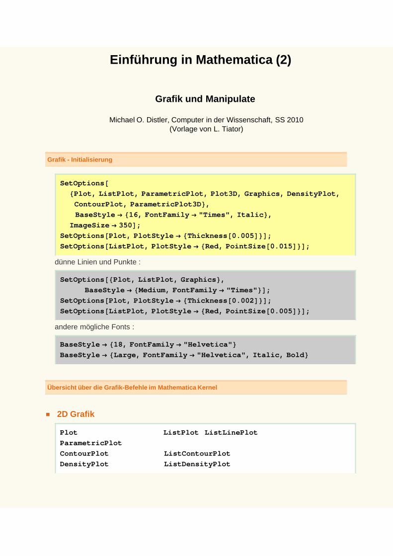
PlotA9x2, Sin@xD, Cos@xD, ãx=, 8x, 0, 2 Π<E
1 2 3 4 5 6
10
20
30
40
50
60
Das Aussehen der Plots kann auf vielfältige Weise durch "Optionen" verändert werden. Diese Optionen haben Voreinstellungen,
können aber auch einzeln manuell verändert werden.
Eine Übersicht gibt die Online-Help oder wie folgt:
Information@"Plot", LongForm ® TrueD
Plot@ f , 8x, xmin, xmax<D generates a plot of f as a function of x from xmin to xmax.
Plot@8 f1, f2, …<, 8x, xmin, xmax<D plots several functions fi.
Attributes@PlotD = 8HoldAll, Protected<Options@PlotD := 9AlignmentPoint ® Center, AspectRatio ®
1
GoldenRatio, Axes ® True, AxesLabel ® None,
AxesOrigin ® Automatic, AxesStyle ® 8<, Background ® None, BaselinePosition ® Automatic,
BaseStyle ® 816, FontFamily ® Times, Italic<, ClippingStyle ® None, ColorFunction ® Automatic,
ColorFunctionScaling ® True, ColorOutput ® Automatic, ContentSelectable ® Automatic,
CoordinatesToolOptions ® Automatic, DisplayFunction ¦ $DisplayFunction, Epilog ® 8<,Evaluated ® Automatic, EvaluationMonitor ® None, Exclusions ® Automatic, ExclusionsStyle ® None,
Filling ® None, FillingStyle ® Automatic, FormatType ¦ TraditionalForm, Frame ® False,
FrameLabel ® None, FrameStyle ® 8<, FrameTicks ® Automatic, FrameTicksStyle ® 8<,GridLines ® None, GridLinesStyle ® 8<, ImageMargins ® 0., ImagePadding ® All,
ImageSize ® 350, ImageSizeRaw ® Automatic, LabelStyle ® 8<, MaxRecursion ® Automatic,
Mesh ® None, MeshFunctions ® 8ð1 &<, MeshShading ® None, MeshStyle ® Automatic,
Method ® Automatic, PerformanceGoal ¦ $PerformanceGoal, PlotLabel ® None,
PlotPoints ® Automatic, PlotRange ® 8Full, Automatic<, PlotRangeClipping ® True,
PlotRangePadding ® Automatic, PlotRegion ® Automatic, PlotStyle ® [email protected]<,PreserveImageOptions ® Automatic, Prolog ® 8<, RegionFunction ® HTrue &L,RotateLabel ® True, Ticks ® Automatic, TicksStyle ® 8<, WorkingPrecision ® MachinePrecision=
Mathematica_2.nb 3
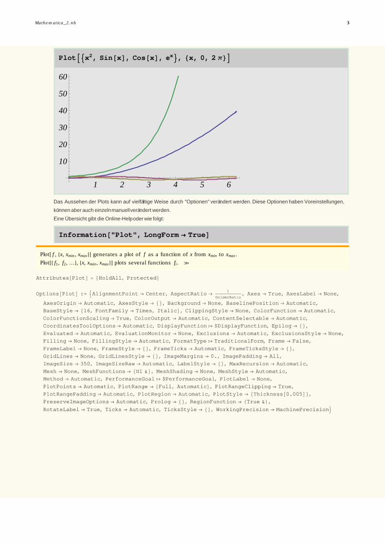
pl1 = Plot@Sin@xD, 8x, 0, 2 Π<, PlotStyle ® Thick,
PlotLabel ® "Die Sinus-Funktion", AxesLabel ® 8"x", "Sin@xD"<D
1 2 3 4 5 6x
- 1.0
- 0.5
0.5
1.0Sin@xD
Die Sinus-Funktion
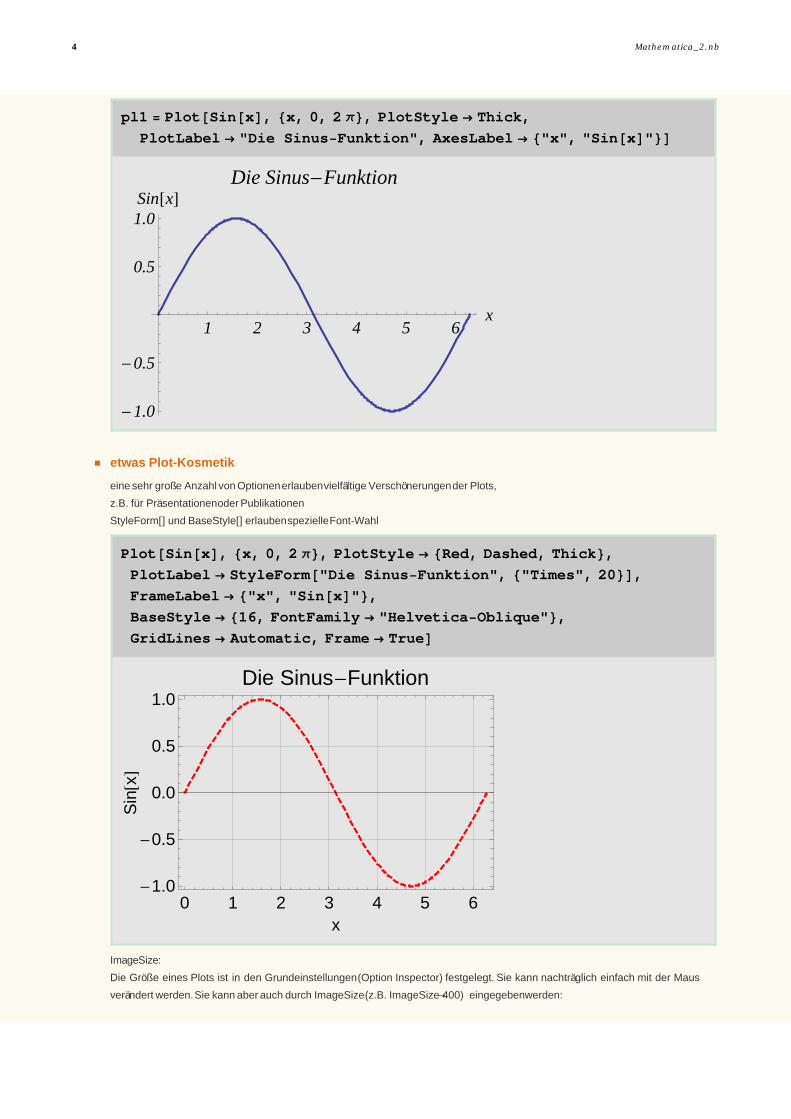
etwas Plot-Kosmetik
eine sehr große Anzahl von Optionen erlauben vielfältige Verschönerungen der Plots,
z.B. für Präsentationen oder Publikationen
StyleForm[ ] und BaseStyle[ ] erlauben spezielle Font-Wahl
Plot@Sin@xD, 8x, 0, 2 Π<, PlotStyle ® 8Red, Dashed, Thick<,PlotLabel ® StyleForm@"Die Sinus-Funktion", 8"Times", 20<D,FrameLabel ® 8"x", "Sin@xD"<,BaseStyle ® 816, FontFamily ® "Helvetica-Oblique"<,GridLines ® Automatic, Frame ® TrueD
0 1 2 3 4 5 6-1.0
-0.5
0.0
0.5
1.0
x
Sin
@xD
Die Sinus-Funktion
ImageSize:
Die Größe eines Plots ist in den Grundeinstellungen (Option Inspector) festgelegt. Sie kann nachträglich einfach mit der Maus
verändert werden. Sie kann aber auch durch ImageSize (z.B. ImageSize®400) eingegeben werden:
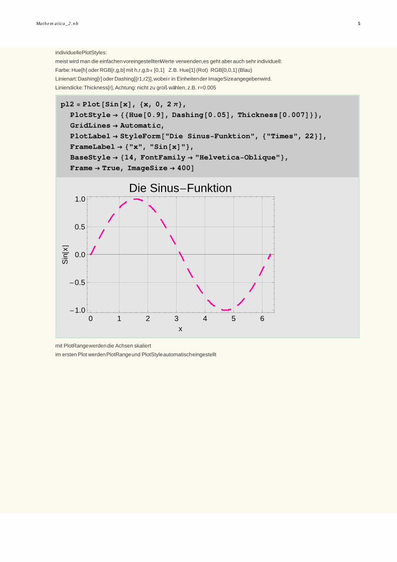
individuelle PlotStyles:
meist wird man die einfachen voreingestellten Werte verwenden, es geht aber auch sehr individuell:
Farbe: Hue[h] oder RGB[r,g,b] mit h,r,g,b Ε [0,1] Z.B. Hue[1] (Rot) RGB[0,0,1] (Blau)
Linienart: Dashing[r] oder Dashing[r1,r2], wobei r in Einheiten der ImageSize angegeben wird.
Liniendicke: Thickness[r], Achtung: nicht zu groß wählen, z.B. r=0.005
4 Mathematica_2.nb
individuelle PlotStyles:
meist wird man die einfachen voreingestellten Werte verwenden, es geht aber auch sehr individuell:
Farbe: Hue[h] oder RGB[r,g,b] mit h,r,g,b Ε [0,1] Z.B. Hue[1] (Rot) RGB[0,0,1] (Blau)
Linienart: Dashing[r] oder Dashing[r1,r2], wobei r in Einheiten der ImageSize angegeben wird.
Liniendicke: Thickness[r], Achtung: nicht zu groß wählen, z.B. r=0.005
pl2 = Plot@Sin@xD, 8x, 0, 2 Π<,PlotStyle ® [email protected], [email protected], [email protected]<<,GridLines ® Automatic,
PlotLabel ® StyleForm@"Die Sinus-Funktion", 8"Times", 22<D,FrameLabel ® 8"x", "Sin@xD"<,BaseStyle ® 814, FontFamily ® "Helvetica-Oblique"<,Frame ® True, ImageSize ® 400D
0 1 2 3 4 5 6-1.0
-0.5
0.0
0.5
1.0
x
Sin
@xD
Die Sinus-Funktion
mit PlotRange werden die Achsen skaliert
im ersten Plot werden PlotRange und PlotStyle automatisch eingestellt
Mathematica_2.nb 5

pl3 = Plot@8Sin@xD, Cos@xD, Tan@xD, Cot@xD<, 8x, 0, 2 Π<,PlotRange ® 8Automatic<, PlotStyle ® 8Automatic<,PlotLabel ® "Sin, Cos, Tan, Cot", FrameLabel ® 8"x", None<,BaseStyle ® 818, FontFamily ® "Helvetica"<, Frame ® TrueD
0 1 2 3 4 5 6
-3-2-1
01234
x
Sin, Cos, Tan, Cot
im nächsten Plot wird die y - Achse neu skaliert und die Linien individuell gewählt
Beachte auch die Funktion Tooltip[ ]
pl3 = Plot@Tooltip@8Sin@xD, Cos@xD, Tan@xD, Cot@xD<D, 8x, 0, 2 Π<,PlotRange ® 8-2, 2<, PlotStyle ®
88Black, Thick<, 8Red, Thick<, 8Blue, Thick<, 8Green, Thick<<,PlotLabel ® "Sin, Cos, Tan, Cot", FrameLabel ® 8"x", None<,BaseStyle ® 818, FontFamily ® "Helvetica"<, Frame ® TrueD
0 1 2 3 4 5 6-2
-1
0
1
2
x
Sin, Cos, Tan, Cot
Show und PlotRange
6 Mathematica_2.nb

Show und PlotRange
f@a_, x_D :=Sin@a xD2
Π Ha x2L
del1 = Plot@f@2, xD, 8x, -2, 2<D
- 2 - 1 1 2
0.1
0.2
0.3
0.4
0.5
0.6
del2 = Plot@f@10, xD, 8x, -2, 2<, PlotRange ® AllD
- 2 - 1 1 2
0.5
1.0
1.5
2.0
2.5
3.0
Mit der Funktion "Show" können bereits existierende Grafiken mit geänderten Optionen dargestellt werden oder auch verschiedene
Grafiken in ein Bild gezeichnet werden.
Mathematica_2.nb 7

Show@del2, PlotRange ® AutomaticD
- 2 - 1 1 2
0.05
0.10
0.15
0.20
del3 = Plot@f@20, xD, 8x, -2, 2<, PlotRange ® AllD
- 2 - 1 1 2
1
2
3
4
5
6
Show@8del1, del2, del3<, PlotRange ® AllD
- 2 - 1 1 2
1
2
3
4
5
6
ListPlot
8 Mathematica_2.nb

ListPlot
ListPlot@8y1, y2, y3, ...<Doder ListPlot@88x1, y1<, 8x2, y2<, ...<D
Kennt man von einer Funktion nur einzelne Punkte oder Wertepaare, kann man diese Funktion nicht mit "Plot" zeichnen. Dafür gibt
es die Funktion "ListPlot" mit ähnlichen Optionen wie Plot.
li1 = RandomReal@80, 1<, 100D;
ListPlot@li1D
20 40 60 80 100
0.2
0.4
0.6
0.8
1.0
[email protected], 8x, 0, 100<D
20 40 60 80 100
0.2
0.4
0.6
0.8
1.0
Mathematica_2.nb 9

Show@%, %%D
20 40 60 80 100
0.2
0.4
0.6
0.8
1.0
lp1 = ListPlot@li1, PlotStyle ® [email protected]
20 40 60 80 100
0.2
0.4
0.6
0.8
1.0
es können auch festdefinierte Werte mit PointSize verwendet werden :
PointSize[Large], PointSize[Small], PointSize[Tiny],
Als weitere Option gibt es im Vergleich zu Plot die Option: PlotJoined->True, wo die einzelnen Punkte durch Linien verbunden
werden:
10 Mathematica_2.nb

ListPlot@li1, Joined ® TrueD
20 40 60 80 100
0.2
0.4
0.6
0.8
1.0
ListLinePlot@li1, Filling ® AxisD
20 40 60 80 100
0.2
0.4
0.6
0.8
1.0
Mit "Show" können nun beide Darstellungen, Linien und Punkte überlagert werden:
Mathematica_2.nb 11

Show@8%, lp1<D
20 40 60 80 100
0.2
0.4
0.6
0.8
1.0
ListPlot@Table@RandomReal@80, 1<, 2D, 83000<DD
0.2 0.4 0.6 0.8 1.0
0.2
0.4
0.6
0.8
1.0
12 Mathematica_2.nb

ParametricPlot
ParametricPlot@8Sin@tD, Cos@tD<, 8t, 0, 2 Π<D
- 1.0 - 0.5 0.5 1.0
- 1.0
- 0.5
0.5
1.0
ParametricPlot@8Sin@7 tD Cos@tD, Sin@5 tD Sin@tD<, 8t, 0, 2 Π<D
- 1.0 - 0.5 0.5 1.0
- 0.5
0.5
1.0
Mathematica_2.nb 13
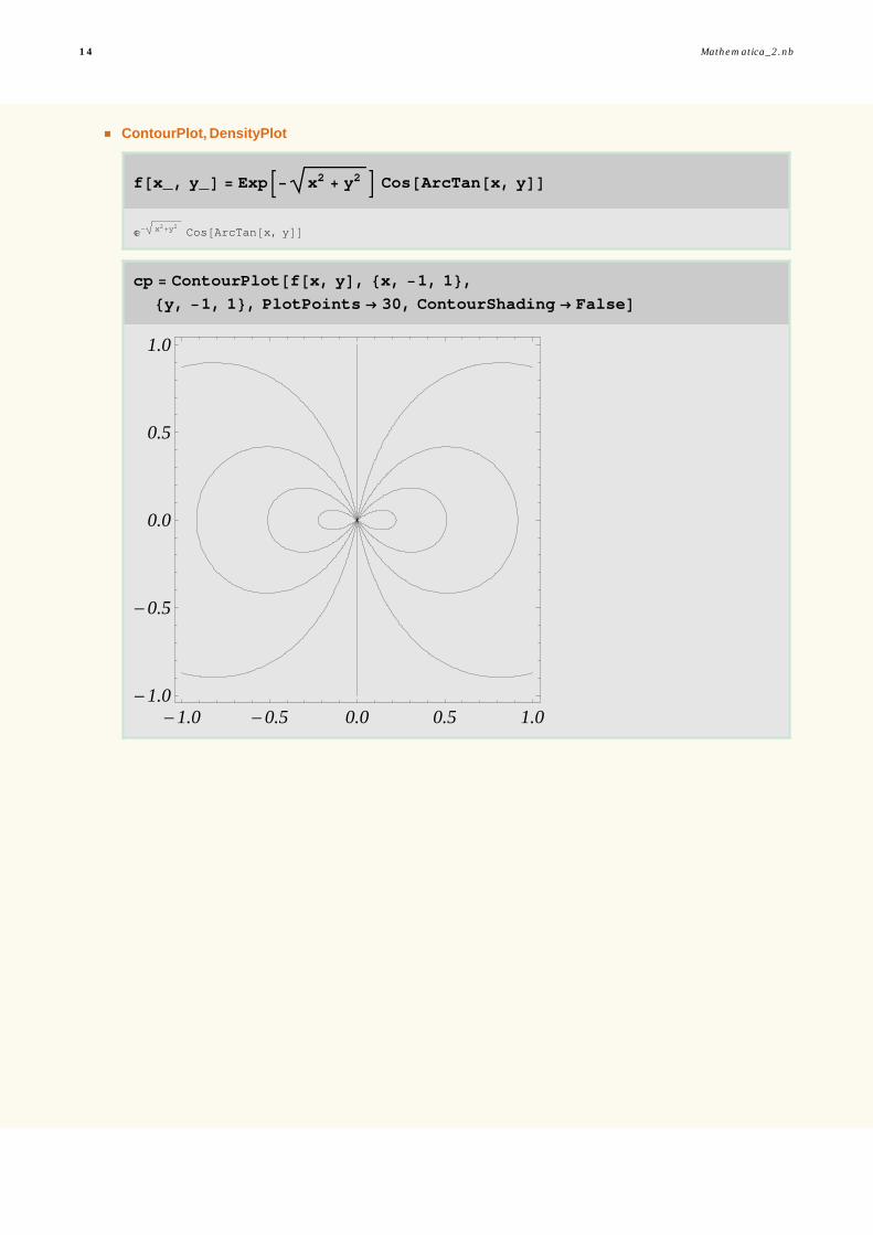
ContourPlot, DensityPlot
f@x_, y_D = ExpB- x2 + y2 F Cos@ArcTan@x, yDD
ã- x2+y2 Cos@ArcTan@x, yDD
cp = ContourPlot@f@x, yD, 8x, -1, 1<,8y, -1, 1<, PlotPoints ® 30, ContourShading ® FalseD
- 1.0 - 0.5 0.0 0.5 1.0- 1.0
- 0.5
0.0
0.5
1.0
14 Mathematica_2.nb

dp = DensityPlot@f@x, yD, 8x, -1, 1<, 8y, -1, 1<,PlotPoints ® 30, Mesh ® False, ColorFunction ® Hue,
Axes ® True, Ticks ® Automatic, Frame ® FalseD
- 1.0 - 0.5 0.5 1.0
- 1.0
- 0.5
0.5
1.0
für andere Farbschemata siehe : ColorSchemes
gemeinsame Darstellung mit GraphicsRow
GraphicsRow@8cp, dp<, PlotLabel ® Exp@-rD Cos@ΒD, ImageSize ® 400D
- 1.0 - 0.5 0.0 0.5 1.0- 1.0
- 0.5
0.0
0.5
1.0
- 1.0 - 0.5 0.5 1.0
- 1.0
- 0.5
0.5
1.0
ã -r cosH Β L
einfachste Anordnung als Liste
Mathematica_2.nb 15
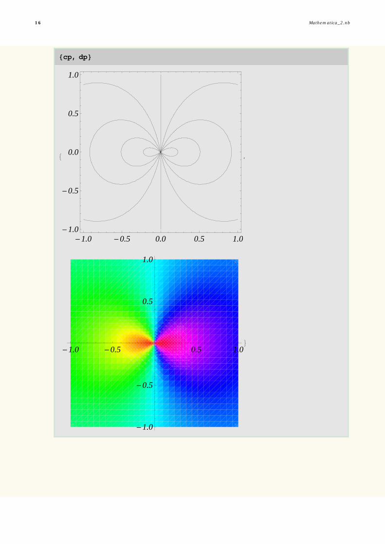
8cp, dp<
9
- 1.0 - 0.5 0.0 0.5 1.0- 1.0
- 0.5
0.0
0.5
1.0
,
- 1.0 - 0.5 0.5 1.0
- 1.0
- 0.5
0.5
1.0
=
16 Mathematica_2.nb

ã GraphicsRow, GraphicsColumn, GraphicsGrid
GraphicsRow@8cp, dp<D
- 1.0- 0.5 0.0 0.5 1.0- 1.0
- 0.5
0.0
0.5
1.0
- 1.0 - 0.5 0.5 1.0
- 1.0
- 0.5
0.5
1.0
GraphicsColumn@8cp, dp<D;
GraphicsGrid@88cp, dp<, 8dp, cp<<D
- 1.0- 0.5 0.0 0.5 1.0- 1.0
- 0.5
0.0
0.5
1.0
- 1.0 - 0.5 0.5 1.0
- 1.0
- 0.5
0.5
1.0
- 1.0 - 0.5 0.5 1.0
- 1.0
- 0.5
0.5
1.0
- 1.0- 0.5 0.0 0.5 1.0- 1.0
- 0.5
0.0
0.5
1.0
Mathematica_2.nb 17

Legenden
selbstdefinierte Legende mit Epilog (aus Mathematica Documentation Center)
legendPlot@xl_List, d_, args___D := Plot@xl, d,
Epilog ® Inset@Panel@Grid@MapIndexed@8Graphics@8ColorData@1, Firstð2D,
Thick, Line@880, 0<, 81, 0<<D<,AspectRatio ® .1, ImageSize ® 20D, ð1< &, xlDDD,
Offset@8-2, -2<, Scaled@81, 1<DD, 8Right, Top<D, argsD
legendPlot@8Sin@xD, Cos@xD, Sinc@xD<, 8x, 0, 10<D
2 4 6 8 10
- 1.0
- 0.5
0.5
1.0sinHx LcosHx LsincHx L
Paket : PlotLegend
Needs@"PlotLegends`"D
18 Mathematica_2.nb

Plot@8Sin@xD, Cos@xD<, 8x, 0, 2 Pi<,PlotLegend ® 8"sine", "cosine"<D
1 2 3 4 5 6
- 1.0
- 0.5
0.5
1.0
cosine
sine
ShowLegend@DensityPlot@Sin@x yD, 8x, 0, Π<, 8y, 0, Π<, Mesh ® False,
PlotPoints ® 30D, 8ColorData@"LakeColors"D@1 - ð1D &,
10, " 1", "-1", LegendPosition ® 81.1, -.4<<D
0.0 0.5 1.0 1.5 2.0 2.5 3.00.0
0.5
1.0
1.5
2.0
2.5
3.0
-1
1
Es gibt eine Vielzahl von Color Schemes, siehe Help
contour1 =
ContourPlot@f@x, yD, 8x, -1, 1<, 8y, -1, 1<, PlotPoints ® 30D;
Mathematica_2.nb 19

ShowLegend@contour1,8ColorData@"LakeColors"D@1 - ð1D &,
10, "1", "-1", LegendSize ® 80.55, 1.35<,LegendLabel ® "Legende",
LegendPosition ® 81.1, -.7<<D
- 1.0 - 0.5 0.0 0.5 1.0- 1.0
- 0.5
0.0
0.5
1.0
-1
1Legende
ShowLegend@ContourPlot@f@x, yD, 8x, -1, 1<,8y, -1, 1<, PlotPoints ® 30, ColorFunction -> "Rainbow",
Contours ® 11, ContourLabels ® AutomaticD,8ColorData@"Rainbow"D@1 - ð1D &, 9, "0.80",
"-0.80", LegendSize ® 80.55, 1.35<,LegendLabel ® "Legende",
LegendPosition ® 81.1, -.7<<D
- 1.0 - 0.5 0.0 0.5 1.0- 1.0
- 0.5
0.0
0.5
1.0
-0.80
0.80Legende
3D-Grafik
20 Mathematica_2.nb

3D-Grafik
Plot3D
Plot3D@f, 8x, xmin, xmax<, 8y, ymin, ymax<DMit "Plot3D" erzeugt man eine Oberflächen-Grafik einer 2-dim Funktion
pl3 = Plot3D@Sin@x + Sin@yDD, 8x, -Π, Π<, 8y, -Π, Π<D
- 2
0
2
- 2
0
2
- 1.0- 0.5
0.00.51.0
pl3 = Plot3D@Sin@x + Sin@yDD, 8x, -Π, Π<,8y, -Π, Π<, Mesh ® False, PlotPoints ® 100D
- 2
0
2
- 2
0
2
- 1.0- 0.5
0.00.51.0
Mit einer Vielzahl von Optionen lassen sich auch diese 3-dim Grafiken verändern,
siehe Options[Plot3D] oder mit Online-Help.
Mathematica_2.nb 21

pl4 = Plot3D@Sin@x + Sin@yDD, 8x, -Π, Π<, 8y, -Π, Π<,AxesLabel ® 8"x", "y", " "<, AxesStyle ® [email protected],AxesEdge ® 8Automatic, Automatic, 81, -1<<,BoxStyle ® [email protected], 0.02<D, PlotLabel ® "sinHx+sinHyLL",BaseStyle ® 816, FontFamily ® "Helvetica"<D
sinHx+sinHyLL
-2
0
2x -2
0
2
y
-1.0-0.50.00.51.0
ParametricPlot3D
z.B. Phasenraumdiagramm einer gedämpften Schwingung
22 Mathematica_2.nb

ParametricPlot3D@[email protected] tD Sin@2 tD, [email protected] tD Cos@2 tD, t10<, 8t, 0, 25<D
- 0.50.0
0.5
- 0.5
0.0
0.5
1.0
0
1
2
parametrisierte Oberfläche
Mathematica_2.nb 23
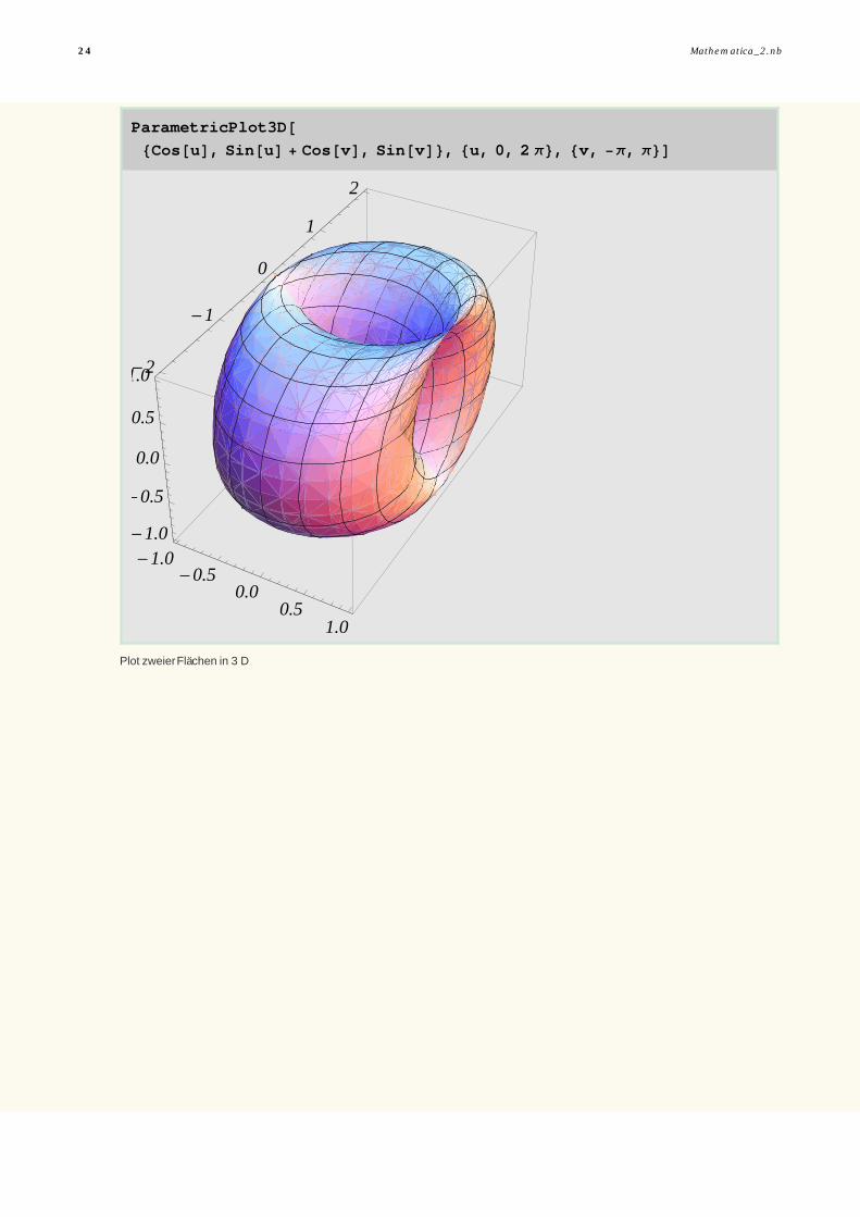
ParametricPlot3D@8Cos@uD, Sin@uD + Cos@vD, Sin@vD<, 8u, 0, 2 Π<, 8v, -Π, Π<D
- 1.0- 0.5
0.00.5
1.0
- 2
- 1
0
1
2
- 1.0
- 0.5
0.0
0.5
1.0
Plot zweier Flächen in 3 D
24 Mathematica_2.nb

ParametricPlot3D@884 + H3 + Cos@vDL Sin@uD, 4 + H3 + Cos@vDL Cos@uD, 4 + Sin@vD<,
88 + H3 + Cos@vDL Cos@uD,3 + Sin@vD, 4 + H3 + Cos@vDL Sin@uD<<,
8u, 0, 2 Pi<, 8v, 0, 2 Pi<,PlotStyle ® 8Red, Green<D
0
5
10
02
46
8
0
2
4
6
8
weitere Grafik-Befehle
LogPlot ListLogPlot
LogLinearPlot ListLogLinearPlot
LogLogPlot ListLogLogPlot
PolarPlot ListPolarPlot
Logarithmische Plots
g@x_D := If@x == 0, 1, xxD
Mathematica_2.nb 25
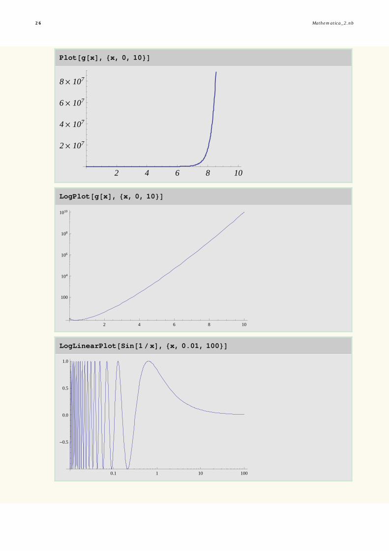
Plot@g@xD, 8x, 0, 10<D
2 4 6 8 10
2 ´ 107
4 ´ 107
6 ´ 107
8 ´ 107
LogPlot@g@xD, 8x, 0, 10<D
2 4 6 8 10
100
104
106
108
1010
LogLinearPlot@Sin@1xD, 8x, 0.01, 100<D
0.1 1 10 100
-0.5
0.0
0.5
1.0
26 Mathematica_2.nb

LogLogPlotAx3 + x13, 8x, 0.1, 100<E
0.5 1.0 5.0 10.0 50.0 100.0
100
107
1012
1017
1022
FilledPlot wird zur Option: Filling -> ...
Table@Plot@Sin@xD, 8x, 0, 2 Pi<, ImageSize ® 150, Filling ® fD,8f, 8Top, Bottom, Axis, 0.3<<D
91 2 3 4 5 6
- 1.0- 0.5
0.51.0
,
1 2 3 4 5 6
- 1.0- 0.5
0.51.0
,
1 2 3 4 5 6
- 1.0- 0.5
0.51.0
,
1 2 3 4 5 6
- 1.0- 0.5
0.51.0
=
Mathematica_2.nb 27

TableAPlotA9x2, Sin@xD, Tan@xD=,8x, -5, 5<, ImageSize ® 200, Filling ® fE,
8f, 8Axis, 83<, 81 -> 82<<, 82 -> 83<<<<E
9- 4 - 2 2 4
- 10- 5
51015
,
- 4 - 2 2 4
- 10- 5
51015
,
- 4 - 2 2 4
- 10- 5
51015
,
- 4 - 2 2 4
- 10- 5
51015
=
Überlagerung mehrerer Plots im gemeinsamen Koordinatensystem mit Show
Show@[email protected], 8x, 0, 1<D,ListPlot@Table@8RandomReal@D, 2 + RandomReal@D<, 8100<DD<,PlotRange ® 80, 4<D
0.2 0.4 0.6 0.8 1.0
1
2
3
4
bei automatischer Skalierung spielt die Reihenfolge eine entscheidende Rolle:
28 Mathematica_2.nb

Show@[email protected], 8x, 0, 1<D,ListPlot@Table@8RandomReal@D, 2 + RandomReal@D<, 8100<DD<D
0.2 0.4 0.6 0.8 1.0
1
2
3
4
5
Show@8ListPlot@Table@8RandomReal@D, 2 + RandomReal@D<, 8100<DD,[email protected], 8x, 0, 1<D<D
0.2 0.4 0.6 0.8 1.0
2.2
2.4
2.6
2.8
3.0
Mathematica_2.nb 29

PolarPlot
PolarPlot@t, 8t, 0, 4 ´ 2 Π<D
-20 -10 10 20
-20
-10
10
20
30 Mathematica_2.nb

SphericalPlot3D
SphericalPlot3D@Abs@SphericalHarmonicY@2, 0, theta, phiDD,8theta, 0, Π<, 8phi, 0, 2 Π<D
-0.2
0.0
0.2
-0.2
0.0
0.2
-0.5
0.0
0.5
Mathematica_2.nb 31

SphericalPlot3D@Abs@SphericalHarmonicY@2, 0, theta, phiDD,8theta, 0, Π<, 8phi, 0, 2 Π<,Boxed ® False, Axes ® None, Mesh ® NoneD
32 Mathematica_2.nb

SurfaceOfRevolution
PlotB12
- x2 +x4
2, 8x, -1.45, 1.45<F
- 1.5 - 1.0 - 0.5 0.5 1.0 1.5
0.1
0.2
0.3
0.4
0.5
0.6
RevolutionPlot3DB12
- x2 +x4
2, 8x, 0.05, 1.4<,
ViewPoint ® 80.521, -0.962, 1.954<, BoxRatios ® 81, 1, 1<F
-1
0
1
-1
0
1
0.0
0.2
0.4
Mathematica_2.nb 33

Paket: ErrorBarPlots`
Needs@"ErrorBarPlots`"D
?ErrorBarPlots`*
ErrorBarPlots`
ErrorBar ErrorBarFunction ErrorBarPlot ErrorListPlot
im ersten Beispiel sind die Abszissen wieder einfach die natürlichen Zahlen,
die Ordinaten zeigen die i , unabhängig von x !
Der Fehlerbalken wird zufällig ermittelt.
ErrorListPlot@Table@8Sqrt@iD, [email protected]<, 8i, 1, 20, 2<DD
2 4 6 8 10
1
2
3
4
in dem nächsten Beispiel (Normalfall) werden Fehlerbalken mit der Funktion ErrorBar erzeugt
34 Mathematica_2.nb
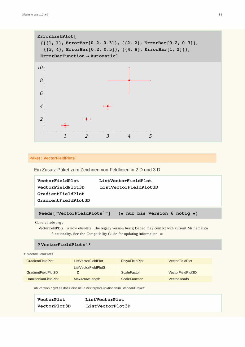
ErrorListPlot@8881, 1<, [email protected], 0.3D<, 882, 2<, [email protected], 0.3D<,
883, 4<, [email protected], 0.5D<, 884, 8<, ErrorBar@1, 2D<<,ErrorBarFunction ® AutomaticD
1 2 3 4 5
2
4
6
8
10
Paket : VectorFieldPlots`
Ein Zusatz-Paket zum Zeichnen von Feldlinien in 2 D und 3 D
VectorFieldPlot ListVectorFieldPlot
VectorFieldPlot3D ListVectorFieldPlot3D
GradientFieldPlot
GradientFieldPlot3D
Needs@"VectorFieldPlots`"D H* nur bis Version 6 nötig *LGeneral::obspkg :
VectorFieldPlots` is now obsolete. The legacy version being loaded may conflict with current Mathematica
functionality. See the Compatibility Guide for updating information.
? VectorFieldPlots`*
VectorFieldPlots`
GradientFieldPlot ListVectorFieldPlot PolyaFieldPlot VectorFieldPlot
GradientFieldPlot3DListVectorFieldPlot3
D ScaleFactor VectorFieldPlot3D
HamiltonianFieldPlot MaxArrowLength ScaleFunction VectorHeads
ab Version 7 gibt es dafür eine neue Vektorplot Funktionen im Standard Paket:
VectorPlot ListVectorPlot
VectorPlot3D ListVectorPlot3D
jedoch funktioniert auch noch das alte Paket
Mathematica_2.nb 35

jedoch funktioniert auch noch das alte Paket
VectorFieldPlot
Vektorfeld einer Zentralkraft FÓ
~rÓrvect = 8x, y, z<8x, y, z<
Fvect = rvect
8x, y, z<
VectorFieldPlot@Take@Fvect, 81, 2<D, 8x, -1, 1<, 8y, -1, 1<D
Vektorfeld einer Axialkraft : FÓ
~rÓ BÓ
Bvect = 80, 0, 1<;Fvect = rvect Bvect
8y, -x, 0<
36 Mathematica_2.nb

VectorFieldPlot@Take@Fvect, 81, 2<D, 8x, -1, 1<, 8y, -1, 1<D
Mathematica_2.nb 37

GradientFieldPlot
GradientFieldPlotB 1
x2 + y2, 8x, -3, 3<, 8y, -3, 3<F
Feldlinien mit konstanter Pfeillänge:
38 Mathematica_2.nb

GradientFieldPlotB 1
x2 + y2,
8x, -3, 3<, 8y, -3, 3.<, ScaleFunction ® H1 &LF
Mathematica_2.nb 39

GradientFieldPlotB 1
x2 + y2, 8x, -3, 3<,
8y, -3, 3<, ScaleFunction ® HLog@ð1D &LF
40 Mathematica_2.nb

GradientFieldPlot3D B 1
Hx - 1L2 + y2 + z2-
1
Hx + 4L2 + y2 + z2,
8x, -5, 5<, 8y, -5, 5<, 8z, -5, 5<, ScaleFunction ® H1 &L,PlotPoints ® 7, VectorHeads ® TrueF
Vektorplot Funktionen im Standard Paket
Ersetzen Paket : VectorFieldPlots` ab Mathematica 7
VectorPlot ListVectorPlot
VectorPlot3D ListVectorPlot3D
VectorFieldPlots`VectorFieldPlot ® VectorPlot
Vektorfeld einer Zentralkraft FÓ
~rÓAlt:
VectorFieldPlot@Take@Fvect,81,2<D, 8x,-1,1<, 8y, -1,1<D
Mathematica_2.nb 41

rvect = 8x, y, z<;Fvect = rvect;
VectorPlot@Take@Fvect, 81, 2<D, 8x, -1, 1<, 8y, -1, 1<D
-1.0 -0.5 0.0 0.5 1.0
-1.0
-0.5
0.0
0.5
1.0
Vektorfeld einer Axialkraft : FÓ
~rÓ BÓ
Alt:
VectorFieldPlot@Take@Fvect,81,2<D, 8x,-1,1<, 8y, -1,1<D
42 Mathematica_2.nb

Bvect = 80, 0, 1<;Fvect = rvect Bvect;
VectorPlot@Take@Fvect, 81, 2<D, 8x, -1, 1<, 8y, -1, 1<D
-1.0 -0.5 0.0 0.5 1.0
-1.0
-0.5
0.0
0.5
1.0
VectorFieldPlots`GradientFieldPlot ® VectorPlot + D(erivative)
Alt:
GradientFieldPlotB1
x2+y2,8x,-3,3<,8y,-3,3<F
Der Gradientvektor muss hier selbst berechnet werden.
Wichtig: Evaluate sorgt für die unmittelbare Berechnung des Gradientvektors
Mathematica_2.nb 43
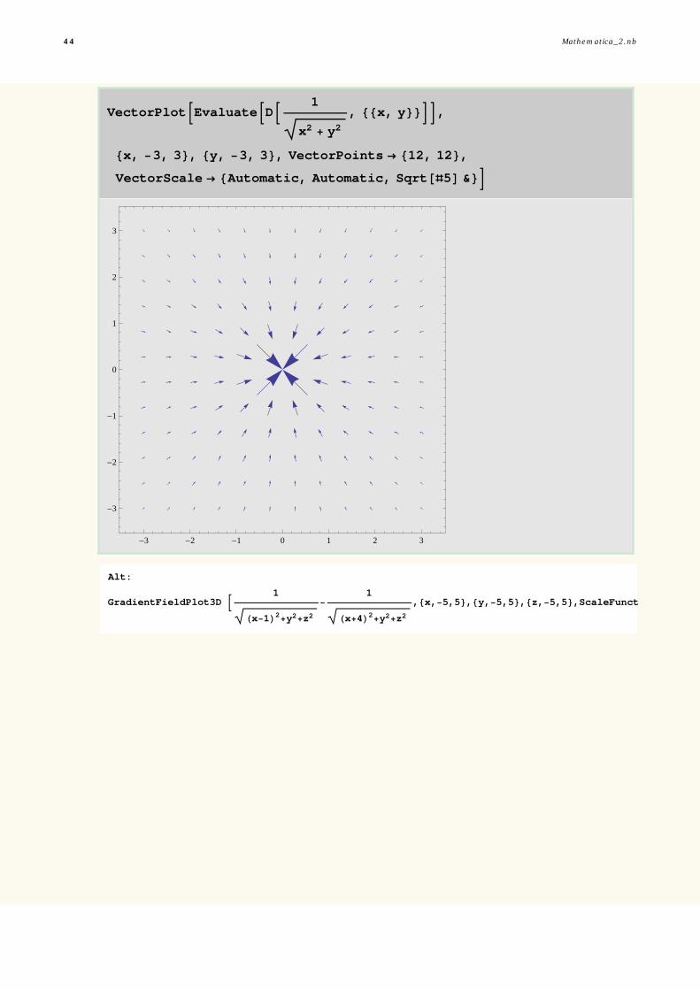
VectorPlotBEvaluateBDB 1
x2 + y2, 88x, y<<FF,
8x, -3, 3<, 8y, -3, 3<, VectorPoints ® 812, 12<,VectorScale ® 8Automatic, Automatic, Sqrt@ð5D &<F
-3 -2 -1 0 1 2 3
-3
-2
-1
0
1
2
3
Alt:
GradientFieldPlot3D B1
Hx-1L2+y2+z2-
1
Hx+4L2+y2+z2,8x,-5,5<,8y,-5,5<,8z,-5,5<,ScaleFunction F
44 Mathematica_2.nb

VectorPlot3DB
DB 1
Hx - 1L2 + y2 + z2-
1
Hx + 4L2 + y2 + z2, 88x, y, z<<F Evaluate,
8x, -5, 5<, 8y, -5, 5<, 8z, -5, 5<,VectorScale ® 8Tiny, Automatic, 1 &<, VectorPoints ® 7F
-5
0
5
-5
0
5
-5
0
5
Mathematica_2.nb 45

Animationen mit Animate
Animate Plot
Animate@Plot@Sin@n xD, 8x, 0, 2 Pi<, Axes ® FalseD,8n, 1, 16<, AnimationRunning ® FalseD
n
46 Mathematica_2.nb
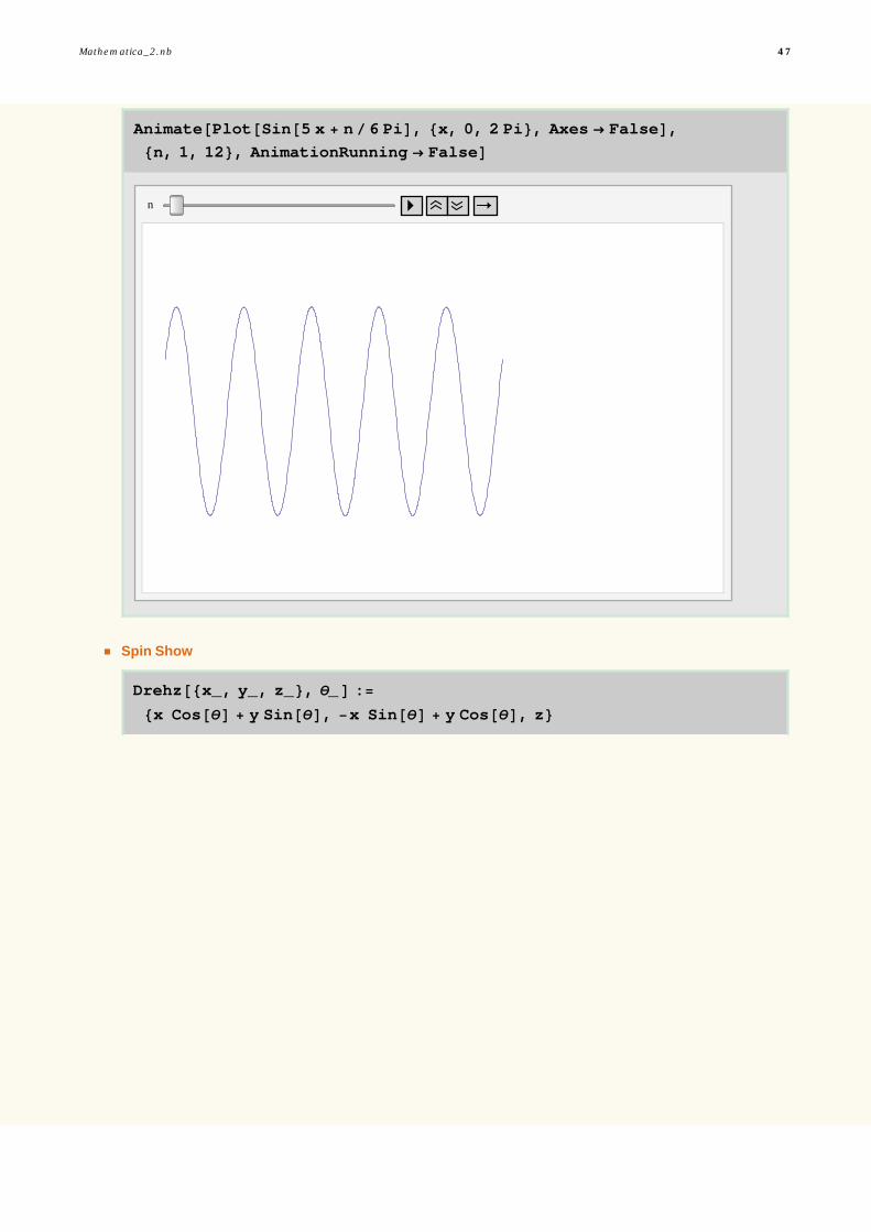
Animate@Plot@Sin@5 x + n6 PiD, 8x, 0, 2 Pi<, Axes ® FalseD,8n, 1, 12<, AnimationRunning ® FalseD
n
Spin Show
Drehz@8x_, y_, z_<, Θ_D :=
8x Cos@ΘD + y Sin@ΘD, -x Sin@ΘD + y Cos@ΘD, z<
Mathematica_2.nb 47

Animate@ParametricPlot3D@Drehz@8x, Cos@tD Sin@xD, Sin@tD Sin@xD<, ΘD,
8x, -Π, Π<, 8t, 0, 2 Π<, Axes ® False, Boxed ® False,
PlotPoints ® 25, PlotRange ® 88-3.2, 3.2<, 8-3.2, 3.2<, 8-1, 1<<D,8Θ, 0, 2 Π<, AnimationRunning ® FalseD
Θ
Manipulate
die beste Neuheit in Mathematica 6
Manipulate[ ] ist so einfach anzuwenden wie Table[ ]
Table@8x, Sin@xD<, 8x, 0, 10<D880, 0<, 81, Sin@1D<, 82, Sin@2D<, 83, Sin@3D<, 84, Sin@4D<,
85, Sin@5D<, 86, Sin@6D<, 87, Sin@7D<, 88, Sin@8D<, 89, Sin@9D<, 810, Sin@10D<<
48 Mathematica_2.nb
Manipulate@8x, Sin@xD<, 8x, 0, 10<D
x
80, 0<
im Allgemeinen werden die Parameter kontinuierlich verändert,
in manchen Fällen ist dies aber nicht so sinnvoll
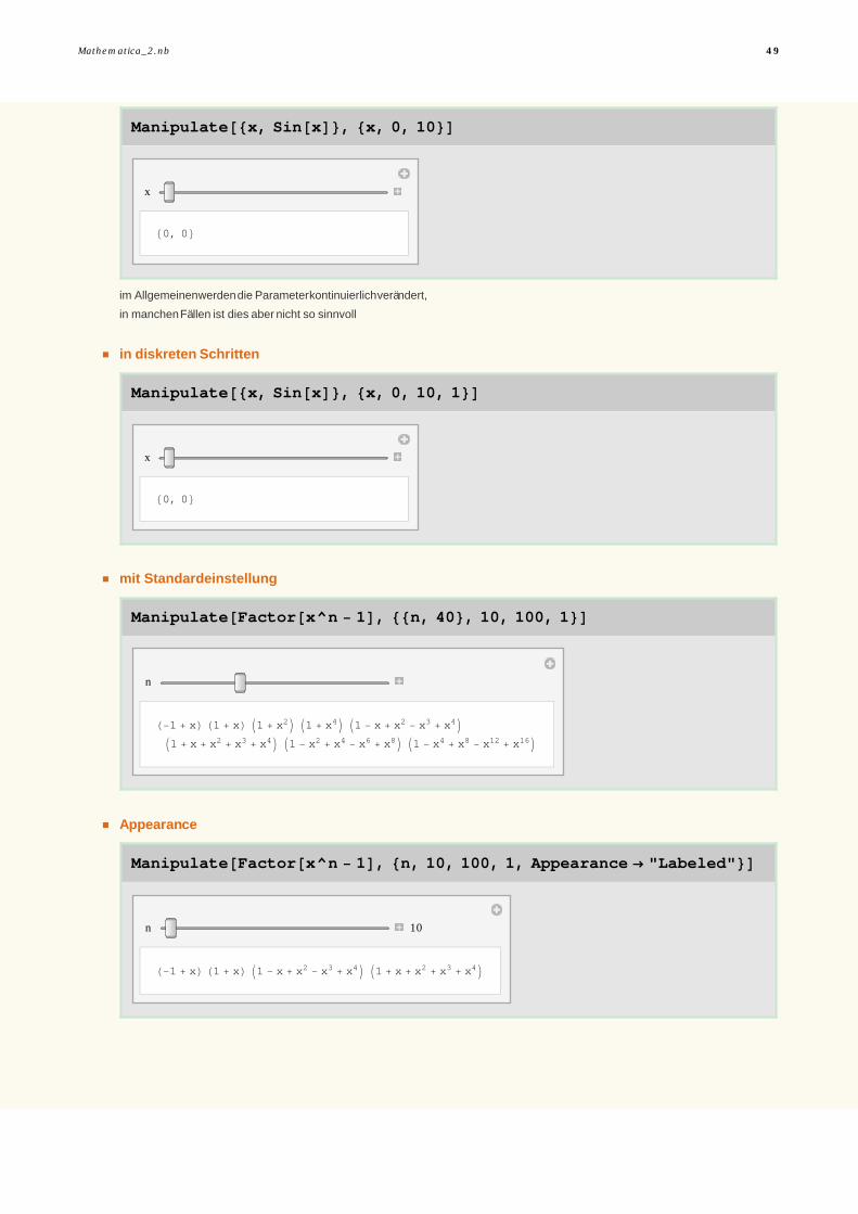
in diskreten Schritten
Manipulate@8x, Sin@xD<, 8x, 0, 10, 1<D
x
80, 0<
mit Standardeinstellung
Manipulate@Factor@x^n - 1D, 88n, 40<, 10, 100, 1<D
n
H-1 + xL H1 + xL I1 + x2M I1 + x4M I1 - x + x2 - x3 + x4MI1 + x + x2 + x3 + x4M I1 - x2 + x4 - x6 + x8M I1 - x4 + x8 - x12 + x16M
Appearance
Manipulate@Factor@x^n - 1D, 8n, 10, 100, 1, Appearance ® "Labeled"<D
n 10
H-1 + xL H1 + xL I1 - x + x2 - x3 + x4M I1 + x + x2 + x3 + x4M
Mathematica_2.nb 49

Manipulate@Factor@x^n - 1D, 8n, 10, 100, 1, Appearance ® "Open"<D
n
10
H-1 + xL H1 + xL I1 - x + x2 - x3 + x4M I1 + x + x2 + x3 + x4M
Table Grids
Manipulate@Grid@Table@8i, i^m<, 8i, 1, n<D, Alignment ® Left,
Frame ® AllD, 88n, 12<, 1, 20, 1<, 88m, 33<, 1, 100, 1<D
n
m
1 1
2 8589934592
3 5559060566555523
4 73786976294838206464
5 116415321826934814453125
6 47751966659678405306351616
7 7730993719707444524137094407
8 633825300114114700748351602 688
9 30903154382632612361920641803 529
10 1000000000000000000000000000 000 000
11 23225154419887808141001767796 309 131
12 410186270246002225336426103 593 500 672
Für die folgenden "manipulierten" Plots wird einheitlich eine etwas kleinere Bildgröße
voreingestellt.
SetOptions@8Plot, ParametricPlot, Graphics<, ImageSize ® 300D;
mehrere Parameter manipulieren
im nachfolgenen Beispiel werden zusätzlich Startparameter definiert :
50 Mathematica_2.nb

Manipulate@Plot@Sin@k x - Ω tD, 8x, 0, 10<D,88k, 2<, 1, 3<, 88Ω, 0.2<, 0, 5<, 8t, 0, 2 Π<D
k
Ω
t
2 4 6 8 10
-1.0
-0.5
0.5
1.0
bei Grafiken ist es oft sinnvoll mit festem PlotRange zu arbeiten:
Manipulate@Plot@Sin@n1 xD + Sin@n2 xD, 8x, 0, 2 Pi<, PlotRange ® 2D,88n1, 14<, 1, 20<, 88n2, 2<, 1, 20<D
n1
n2
1 2 3 4 5 6
-2
-1
1
2
Mathematica_2.nb 51

Radio Buttons und Pop-up Menüs
Manipulate@Plot@Sin@n1 xD + Sin@n2 xD, 8x, 0, 2 Pi<,Filling ® filling, PlotRange ® 2D, 88n1, 8<, 1, 20<,
88n2, 13<, 1, 20<, 8filling, 8None, Axis, Top, Bottom<<D
n1
n2
filling None Axis Top Bottom
1 2 3 4 5 6
-2
-1
1
2
wenn die Auswahl zu groß wird, erscheint automatisch ein Pop-Up Menü
52 Mathematica_2.nb

Manipulate@Plot@Sin@n1 xD + Sin@n2 xD,8x, 0, 2 Pi<, Filling ® filling, PlotRange ® 2D,
8n1, 1, 20<, 8n2, 1, 20<, 8filling,8None, Axis, Top, Bottom, Automatic, 1, 0.5, 0, -0.5, -1<<D
n1
n2
filling None
1 2 3 4 5 6
-2
-1
1
2
Mathematica_2.nb 53

Checkbox für True und False
Manipulate@Plot@Sin@n1 xD + Sin@n2 xD, 8x, 0, 2 Pi<, Frame ® frame,
PlotRange ® 2D, 8n1, 1, 20<, 8n2, 1, 20<, 8frame, 8True, False<<D
n1
n2
frame
0 1 2 3 4 5 6-2
-1
0
1
2
Anfangswerte und Labels
Ein schönes Beispiel mit Lissajous Kurven
app = Appearance ® "Labeled";
54 Mathematica_2.nb

Manipulate@ParametricPlot@8a1 Sin@n1 Hx + p1LD, a2 Cos@n2 Hx + p2LD<,8x, 0, 20 Pi<, PlotRange ® 1, PerformanceGoal ® "Quality"D,
88n1, 1, "Frequency 1"<, 1, 4, app<,88a1, 1, "Amplitude 1"<, 0, 1, app<,88p1, 0, "Phase 1"<, 0, 2 Pi, app<,88n2, 54, "Frequency 2"<, 1, 4, app<,88a2, 1, "Amplitude 2"<, 0, 1, app<,88p2, 0, "Phase 2"<, 0, 2 Pi, app<D
Frequency 1 1
Amplitude 1 1
Phase 1 0
Frequency 25
4
Amplitude 2 1
Phase 2 0
-1.0 -0.5 0.5 1.0
-1.0
-0.5
0.5
1.0
die Empfindlichkeit der Regler kann erheblich gesteigert werden :
mit der Alt Taste um Faktor 20, mit Alt+Ctrl um Faktor 400
mit mit Alt+Ctrl+Shift um Faktor 8000
Mathematica_2.nb 55
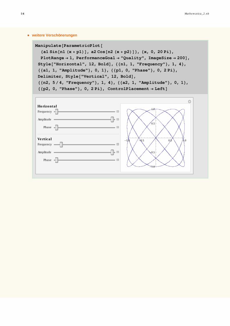
weitere Verschönerungen
Manipulate@ParametricPlot@8a1 Sin@n1 Hx + p1LD, a2 Cos@n2 Hx + p2LD<, 8x, 0, 20 Pi<,PlotRange ® 1, PerformanceGoal ® "Quality", ImageSize ® 200D,
Style@"Horizontal", 12, BoldD, 88n1, 1, "Frequency"<, 1, 4<,88a1, 1, "Amplitude"<, 0, 1<, 88p1, 0, "Phase"<, 0, 2 Pi<,Delimiter, Style@"Vertical", 12, BoldD,88n2, 54, "Frequency"<, 1, 4<, 88a2, 1, "Amplitude"<, 0, 1<,88p2, 0, "Phase"<, 0, 2 Pi<, ControlPlacement ® LeftD
Horizontal
Frequency
Amplitude
Phase
Vertical
Frequency
Amplitude
Phase
-1.0 -0.5 0.5 1.0
-1.0
-0.5
0.5
1.0
56 Mathematica_2.nb

2 D Sliders
Manipulate@Graphics@8Line@Table@88Cos@tD, Sin@tD<, pt<,8t, 2. Pin, 2. Pi, 2. Pin<DD<, PlotRange ® 1D,
88n, 50<, 1, 200, 1<, 88pt, 80, 0<<, 8-1, -1<, 81, 1<<D
n
pt
Mathematica_2.nb 57

Locators
Manipulate@Graphics@8Line@Table@88Cos@tD, Sin@tD<, pt<, 8t, 2. Pin, 2. Pi, 2. Pin<DD<,
PlotRange ® 1D, 88n, 30<, 1, 200, 1<, 88pt, 80, 0<<, Locator<D
n
ã Polynom durch n Punkte
mit Strg - Alt - Klick lassen sich Punkte sowohl hinzufügen als auch löschen
58 Mathematica_2.nb
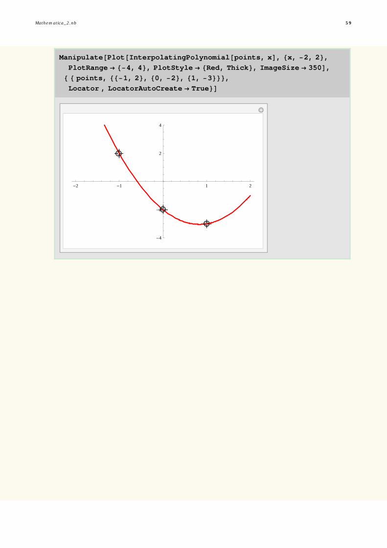
Manipulate@Plot@InterpolatingPolynomial@points, xD, 8x, -2, 2<,PlotRange ® 8-4, 4<, PlotStyle ® 8Red, Thick<, ImageSize ® 350D,
8 8 points, 88-1, 2<, 80, -2<, 81, -3<<<,Locator , LocatorAutoCreate ® True<D
-2 -1 1 2
-4
-2
2
4
Mathematica_2.nb 59