Eindhoven University of Technology

MASTER

A feasibility study of a free piston compressor with linear motor

Jacobs, J.A.H.M.

Award date:1990

Link to publication

DisclaimerThis document contains a student thesis (bachelor's or master's), as authored by a student at Eindhoven University of Technology. Studenttheses are made available in the TU/e repository upon obtaining the required degree. The grade received is not published on the documentas presented in the repository. The required complexity or quality of research of student theses may vary by program, and the requiredminimum study period may vary in duration.

General rightsCopyright and moral rights for the publications made accessible in the public portal are retained by the authors and/or other copyright ownersand it is a condition of accessing publications that users recognise and abide by the legal requirements associated with these rights.

• Users may download and print one copy of any publication from the public portal for the purpose of private study or research. • You may not further distribute the material or use it for any profit-making activity or commercial gain

A feasibility study of a free piston compressor with linear motor

WFW 90.062

J.A.H.M. Jacobs

J.A.H.M. Jacobs December 1990

Abstract

Domestic refrigeration equipment is usually supplied with a reciprocating compressor driven by a rotating electric motor. The cooling capacity is normally regulated by means of on/off control. This way of control yields a lower efficiency compared to continuous control. Contin- uous control can be achieved by the use of a so called free piston compressor with a variable stroke. This report deals with a feasibility study of such a free piston compressor with an integrated linear motor. This concept is very attractive compared to other concepts due to its simple construction. The aim of this thesis is to prove the concept by a theoretical and experimental analysis. A first approximation of the generated electromagnetic force has been made with an analytical model of the magnetic circuit. This model proved to be a useful tool to estimate the main dimensions of the motor. A more detailed analysis - including non-linear material behaviour and stray flux effects - has been carried out with the finite element package PE2D. For the dynamic behaviour the compressor can be treated as a mass-spring-damper system. Calculations on this system have been performed with a linear and a non-linear model. Taken into account the results obtained with the theoretical analysis we have realised a pro- totype of a free piston compressor with linear motor. The applied soft magnetic material (corovac) consists of electrically isolated particles resulting in low eddy current losses. A disadvantage of this material is the low magnetic permeability compared to iron. An experimental set-up has been designed to measure the force characteristics. The measured characteristics are in good agreement with the characteristics obtained with the finite ele- ment model. The electric losses have been measured with a fixed rotor. These measurements confirm the low eddy current losses for a motor made of corovac. Although the magnetic properties of corovac do not meet the specifications of the manufac- turer a motor efficiency of 87 % can be reached for an output power of 50 W. The results obtained from the theoretical and experimental analysis show that the free piston compressor as proposed in this report is a promising concept.

Preface

The work presented in this report has been carried out at Philips Research Laboratories at Eindhoven within the research group ’Transport Phenomena’. One section of this group works on domestic refrigeration equipment where I have been employed for one year. Within this group I had the opportunity to do an investigation on a new compressor concept for refrigeration equipment. This investigation is described in this thesis which forms the last part of my Master’s study at the faculty of Mechanical Engineering at the Eindhoven University of Technology.

I wish to thank all the members of the ’refrigeration research group’ who have given me theoretical and experimental support. In particular I appreciate the fruitful discussions and help of Ir. A.A.J. Benschop. In addition I like to thank Mr. C.A.N. van der Meuten for the realisation of the prototype and his many constructive suggestions. Especially for the electro-magnetic analysis I appreciate the support and comments given by Prof.dr.ir E.M.H. Kamerbeek and Ir. F.A. Boon.

F i n d y I wish to thank Philips Research Laboratories for enabling me to do this investigation.

.. 11

Contents

Abstract

Preface

List of Symbols

i Introduction

2 Principle of linear free piston compressor 2.1 Cooling cycle . . . . . . . . . . . . . . . . . . . . . . . . . . . . . . . . . . . . 2.2 Capacity control . . . . . . . . . . . . . . . . . . . . . . . . . . . . . . . . . . 2.3 Free piston compressor . . . . . . . . . . . . . . . . . . . . . . . . . . . . . . .

3 Calculations 3.1 Magnetic Circuit . . . . . . . . . . . . . . . . . . . . . . . . . . . . . . . . . .

3.1.1 Analytical model . . . . . . . . . . . . . . . . . . . . . . . . . . . . . . 3.1.2 Finite element model . . . . . . . . . . . . . . . . . . . . . . . . . . . . 3.1.3 Comparison analytical model and finite element model . . . . . . . . .

3.2 Dynamic behaviour . . . . . . . . . . . . . . . . . . . . . . . . . . . . . . . . . 3.2.1 Linear model . . . . . . . . . . . . . . . . . . . . . . . . . . . . . . . . 3.2.2 Non-linear model . . . . . . . . . . . . . . . . . . . . . . . . . . . . . .

3.3 Electric Circuit . . . . . . . . . . . . . . . . . . . . . . . . . . . . . . . . . . . 3.3.1 Inductance o€ motor . . . . . . . . . . . . . . . . . . . . . . . . . . . . 3.3.2 Coildesign . . . . . . . . . . . . . . . . . . . . . . . . . . . . . . . . . 3.3.3 Electric power losses . . . . . . . . . . . . . . . . . . . . . . . . . . . .

4 Realisation of prototype 4.1 Soft magnetic material . . . . . . . . . . . . . . . . . . . . . . . . . . . . . . . 4.2 Permanent magnets . . . . . . . . . . . . . . . . . . . . . . . . . . . . . . . . 4.3 Coil . . . . . . . . . . . . . . . . . . . . . . . . . . . . . . . . . . . . . . . . . 4.4 Compressor part . . . . . . . . . . . . . . . . . . . . . . . . . . . . . . . . . .

5 Experiments 5.1 Magnetic flux density . . . . . . . . . . . . . . . . . . . . . . . . . . . . . . . 5.2 Force characteristics . . . . . . . . . . . . . . . . . . . . . . . . . . . . . . . . 5.3 Electric losses . . . . . . . . . . . . . . . . . . . . . . . . . . . . . . . . . . . . 5.4 Efficiency . . . . . . . . . . . . . . . . . . . . . . . . . . . . . . . . . . . . . .

i .. 11

Y

1 3 3 4 6

8 8 8

13 16 19 19 23 27 27 28 30

33 34 34 35 36

38 38 38 39 42

6 Conclusions and remarks

... 111

43

Bibliography

Appendices

A Derivation of electromagnetic force

E! Maxwell equations

C Force characteristics obtäined with ~ d y t . i c d mede!

D PE2D input file

E Comparison characteristics OP analytical and finite element model

F Example of a FREEPI run

Samenvatting

Index

44

45

45

49

50

54

56

58

60

61

iv

List of Symbols A Ac B Br d D E f f w F h H i j J k I L m N N i P P R t T U 2

vector potential area of cross section flux density remanence of permanent magnet damping displacement current electric field strength frequency coil space factor force enthalpy magnetic field strength current complex constant ( j 2 = -i) current density stiffness length inductance moving mass number of windings number of ampere turns power pressure magnetic resistance; electric resist an ce time temperature magnetic potential; electric potential axial position

Greek Symbols

dimensionless damping permittivity of vacuum relative permittivity coefficient of adiabatic expansion dimensionless frequency permeability of vacuum relative permeability magnetic flux phase shift frequency (w = 27rf) undamped eigenfrequency damped eigenfrequency charge density resistivity

[ - I

[ - I [ - 1 [ - 1 E - 1 [ W l [ rad I [ rads-' ] [ rad.s-l ] [ rads-' ] [ ] [ Q m l

[ Fm-l ]

[ Hm"' 3

V

Subscripts

C

d e i . i

m

P

e

O

T

S

coil; condenser discharge evaporator inner left inuncta2ce magnet; maximum outer pis ton right; rotor suction amplitude

Conversion table of units

T Wb H V F C

kg

kg m2A-2s-2 kg m2A-1s-3 A2 s4kg- m-2 As

kg m2A-is-2

vi

Chapter 1

Introduction

Philips research activities on domestic refrigeration equipment are concentrated at the Re- search Laboratories in Eindhoven. Within the group 'Transport Phenomena' one section is responsible for the introduction of new concepts concerning domestic refrigeration equipment. The topics dealt within this section are numerical simulation of the cooling cycle, application of new refrigerants and investigations on continuously controlled compressors. The work de- scribed in this thesis deals with the latter area.

In domestic refrigeration equipment usually a reciprocating compressor is applied driven by a rotating electric motor. The rotating movement is converted into a reciprocating movement by a crank mechanism resulting in a fixed stroke of the piston. Normally on/off control is applied to get a variable cooling capacity. This way of control results in thermodynamic and start/stop losses which are approximately 10-20% of the total energy consumption. These losses can be eliminated by the use of continuous control which means that the cooling ca- pacity is adjusted continuously to its demand. One option for continuous control is the use of a compressor with variable frequency. A drawback for this option is that capacity variation is limited due to balancing and valve problems. Another option is the application of a com- pressor with a variable stroke or a so called free piston compressor. During the past years several attempts have been made to design a free piston compressor with an integrated linear motor. These attempts failed due to the high electromagnetic radial forces resulting in a high bearing load and friction. For the present free piston compressor the problems with radial forces are solved by the use of a separate oscillating motor. Evaluation of this an other free piston compressor concepts resulted in a new design with an integrated linear motor. The radial forces are kept to a minimum by the use of large air gaps between rotor and stator. These air gaps are Wed with permanent magnetic material resulting in a big increase of the generated electromagnetic force. The aim of this thesis is to investigate the feasibility of this new compressor concept. The goal for this investigation is to design a motor with an efficiency of 90 % at a nominal delivered mechanical power of 50 W and a running frequency of approximately 50 Hz.

In the next chapter the cooling cycle as applied in domestic refrigeration equipment is ex- plained in some detail. Also the options for cooling capacity control and the principle of the free piston compressor with linear motor are discussed within this chapter.

For the theoretical analysis a distinction is made between the magnetic, dynamic and elec- tric behaviour as shown in chapter 3. The magnetic behaviour has been investigated with an analytical model and a finite element model. A comparison is made between the results

1

obtained with these models. Two models are discussed to predict the dynamic behaviour, a linear analytical model and a non-linear numeric model based on time simulations. The number of windings and wire diameter of the coil can be determined with a simple ana- lytical model as outlined in the last paragraph of this chapter.

Chapter 4 deals with the realisation of the prototypes. The experiiiiznt~ carried ent m these. prototypes are discussed in chapter 5. 'Nithin this diiapiei dm a cûïxparism is made betwen the calculated and measured characteristics.

Findy some conclusions and remarks are given.

2

Principle of linear free piston compressor

For domestic refrigeration equipment the cooling capacity is normally regulated by means of on/off control. A better understanding of the losses caused by this way of control and the advantages of continuous control can be obtained by investigation of the cooling cycle in some detail. One option for continuous control is the use of a free piston compressor with a variable stroke. The free piston concept as described in this report is provided with an integrated linear motor which is attractive due to its simple construction.

The cooling cycle as applied in domestic refrigeration equipment consists of a vapour com- pression cycle or reversed Rankine cycle [SI . A schematic representation of the cycle is given in figure 2.1.

,Capillary

2

N ' compressor

I li-

Figure 2.1: Cooling cycle with pressure-enthalpy diagram

The complete cycle can be divided into four steps which will be discussed in some detail now.

3

o Compression At point 1 of figure 2.1 the refrigerant is in vapour phase with a low pressure. The pressure of the refrigerant is increased by means of a compressor to the pressure level at point 2. At this point the refrigerant is in a superheated vapour phase. Most refrigeration equipment used nowadays is applied with a fixed stroke reciprocating C G Z I ~ S S Q ~ dri,yez by z crank mechanism with electric motor. The compressor with electric motor is mounted in a sealed vessel which is partly filled with oil for iubrication of the bearings.

o Condensation The condensation process takes place between the points 2 and 3. Due to the high pressure the refrigerant has a high saturation temperature, so condensation occurs if the condensor is placed in an ambient with a lower temperature. During the transition &om superheated vapour at point 2 to subcooled liquid at point 3 heat is transported to the ambient. For most refrigeration equipment the condenser can be found at the rear of the cabinet.

o Expansion The expansion from high pressure at point 3 to a low pressure at point 4 is almost isenthalpic (kconstant). Normally a capillary tube is used for the expansion process which is a cheap and reliable solution.

o Evaporation At this stage the actual cooling takes place. Due to the low pressure the refrigerant has a low saturation temperature, so evaporation occurs when the evaporator is placed in an ambient with a higher temperature. The evaporator is mounted inside the cabinet and absorbs heat due to evaporation of the refrigerant from point 4 to point 1.

2.2 Capacity control

The cooling cycle has to be driven in such a way that within the cabinet a requested mean temperature is maintained. The necessary cooling capacity is defined by the heat loss of the cabinet which depends on the requested cabinet temperature and the temperature of the ambient. These boundary conditions of the cooling circuit vary during time so a variable cooling capacity is needed. The options to reach this demand are:

o On/off control This option is most widely used in domestic refrigeration equipment because of its low cost and reliability. A thermostat mounted within the cabinet switches the compressor on or off when a maximum or minimum temperature is reached. This results in a hysteresis around the set temperature. Disadvantages of this way of control are the start/stop losses and thermodynamic losses [SI. The start/stop losses are caused by pressure increase and decrease in the condenser and evaporator. Another effect is the evaporation in the condenser and condensation in the evaporator during the off-period. The thermodynamic losses can be explained by means of the temperature curves for evaporator and condenser given schematically in figure 2.2. For a cooling circuit the efficiency according to Carnot is defined as:

4

r

Figure 2.2: Temperature curves for evaporator and condenser

So to reach a maximum Carnot efficiency it is important to keep the temperature dif- ference between condenser and evaporator as small as possible. For on/off control the heat load of the evaporator and condensor during the on-period is higher compared to a continuously controlled system. This leads to a higher mean temperature difference between evaporator and condensor during the on-period resulting in the so called ther- modynamic losses. The thermodynamic losses and start/stop losses are approximately 10-20 % of the total energy consumption.

o Continuous control Application of continuous control means that the compressor is running continuously. A variable capacity can be achieved by:

- variable stmte The mass flow of the refrigerant caa be varied by variation of the stroke. This solu- tion will be difficult to use in a conventional reciprocating compressor because the movement of the piston is kinematically prescribed. A kinematic free movement of the piston can be obtained by a so called free piston compressor as discussed in next paragraph.

- variable dead volume It is also possible to vary the mass flow by variation of the dead volume. Decreasing the dead volume leads to an increasing mass flow. A difficulty for this way of capacity variation is the controlability.

- variable frequency Theoretical this way of control cm also be used for the conventional reciprocat- ing compressor. In practice several problems arise like balancing problems and valve losses. A possible candidate for frequency control is the rotary compressor although the performance is bad at lower frequency [8].

5

2.3 Free piston compressor

During the past years several attempts have been made to design a free piston compressor with linear motor. AU these attempts failed due to the high radial magnetic forces resulting in a high bearing load and friction. To overcome these problems a free piston compressor has been designed with a separate oscillating motor. The concept is shown in figure 2.3.

Electric Motor

Motor yoke

Ccnnpessor -

I

Permanent magnet

Coil Rotor Dart

Central bearing

Inner Stator Outer stator

Cylinder

Piston

Valve plates

Figure 2.3: Free piston compressor with oscillating motor

During operation the yoke rotates periodically over a small angle around the central bear- ing. This movement results in a reciprocating movement of the piston. The magnetic flux distribution caused by the permanent magnets is indicated with the solid arrows. When the coil is supplied with a DC current a magnetic flux will be imposed as indicated with the dashed arrows. The magnetic flux will be increased at the rotor parts indicated with A and decreased at the rotor parts indicated with B. This results in an anti-clock wise rotation of the yoke which is converted into a movement of the piston to the right. An alternating current through the coil causes the magnetic flux to be increased and decreased alternately at the rotor parts indicated with A and B. This results in a periodic rotation of the yoke and a reciprocating movement of the piston.

The experience and know-how gained with this motor and previous linear motor designs re- sulted in the idea to design a linear motor with relatively large air gaps at the rotor-ends and to fill these air gaps with permanent magnetic material. A cross section of this concept is shown in figure 2.4. Due to the large air gaps the flux distribution will be almost insensitive to small gap vari- ations caused by alignment errors or unroundness of the rotor. As a result of the almost uniform flux distribution the radial forces will be very small. Normally large air gaps result in a decrease of the generated electromagnetic force. However an increase of the electromag- netic force is even possible compared to a motor with small air gaps, by filling the large air gaps at the rotor-ends with permanent magnetic material. The advantage of the low radial forces still holds because permanent magnetic material like ferroxdure [ 11 behaves almost like air with respect to the magnetic resistance. The calculations in next chapter show that an

6

Stator Rotor 4

Coil Permanent magnet

Figure 2.4: Free piston compressor with linear motor

optimum exists for the thickness of the magnetic rings at the rotor-ends. The working principle of the linear motor is almost the same as for the oscillating motor. The coil and permanent magnetic rings are mounted in the stator. The permanent magnetic rings consist of one ring at the center (further called inner magnet) and a smaller ring at left and right side (further called outer magnet). The inner and outer magnets are magnetized in opposite direction resulting in a magnetic flux distribution as indicated with the solid arrows. A DC current through the coil results in a magnetic flux distribution as indicated by the dashed arrows. The imposed flux distribution results in an increase of the magnetic flux at the rotor-end indicated with A and a decrease of the magnetic flux at the rotor-end indicated with B. This results in an electromagnetic force on the rotor part to the right. An alternating current through the coil causes an alternately high and low magnetic flux at the rotor-ends A and B resulting in a reciprocating movement of the rotor. The concept as outlined here is covered by a patent application.

7

Calculations

3.1 Magnetic Circuit

For the design of the linear motor it is necessary to investigate the electro-magnetic behaviour. A first approximation has been made by means of an analytical model. This model can be used to make an estimation for the main dimensions of the motor and to investigate the influence of the design parameters. For the analytical analysis the following assumptions have been made:

o linear behaviour of magnetic material

o no saturation

o no stray f lux

Although these assumptions will result in a considerable error we have the experience that an analysis done in this way gives good insight into the magnetic behaviour qualitatively. A more accurate prediction can be done with a finite element model where non-linear be- haviour of the magnetic material, saturation and stray flux axe taken into account.

3.1.1 Analytica! model

The electric scheme of the magnetic circuit can be found by the definition of magnetic po- tential, resistance and flux as given in appendix A. Usage of these definitions results in the electric scheme as shown in figure 3.1. A cross section of the motor with the relevant param- eters can be found in figure 3.2. The magnetic potentials of the model are:

N i - coil Mi - inner-magnet Mo - outer-magnet

The magnetic resistances are:

Rc - coil 4 s - iron of stator-half 4 r - iron of rotor-half R,,,; - inner-magnet

8

Figure 3.1: Electric scheme of magnetic circuit

Rml - left-magnet Rmr - right-magnet

- air-gap left Rgr - air-gap right Rgi - air-gap inner

The magnetic fluxes are:

4; - inner part &i . - left part h - right part

The electric scheme can be simplified to the scheme given in figure 3.3 by definition of the following resistances:

Application of Kirchhoff’s laws leads to the following set of equations:

R; Ri O M; + Mo - N i l 2

9

axis of symmetry

Figure 3.2: Cross section of motor with design parameters

The package REDUCE 151 is used to solve this set of equations and to carry out the algebraic operations discussed further in this chapter. Solving the matrix equation leads to :

4i =

41 =

d r =

2R?(Mi + Mo) - (2Ri + %)Ni 2(&.Ri 4- &.& + RI&) (3.3)

The electromagnetic force on the rotor can be expressed by next equation as derived in ap- pendix A.

(3-4)

I with j being the source number with flux 4j and magnetic potential Um,. Substitution of the equations for the flux as given in 3.3 together with the defined potentials for the permanent magnets and coil leads to next expression for the generated force on the rotor:

Substitution of the third equation from 3.2 (& = 41 + 4r) leads to:

10

Figure 3.3: Reduced electric scheme of magnetic circuit

To save writing we introduce next parameters referring to the dimensions shown in figure 3.2.

For the calculation of the resulting force only the resistances Rml, Lr, Rgl and R,, are considered as functions of the rotor position x. According to expression A.4 the resistances can be expressed as:

With

The resistances RJ and Rr can now be expressed as:

where

C RI = Ry+- Io - x R, = R y + - 1, + 2

C

(3.9)

11

and

(3.10)

The final expression for the force on the rotor can be found by substitution of the expressions given in 3.3,3.9 and 3.10 into equation 3.6. The pâ,&ge REDGGE fin& the fei^wing sdnf.i^n

Where :

and :

Neglecting the magnetic resistance of the iron parts (R, = O) leads to next expression for the force on the rotor:

Fr = (3.12) c * (Mi + Mo) * Ni- x * & *

(c + 2Rilo)C The first part with term N i is called the hybrid force whereas the second part with term ( N i ) 2 is called the reluctance force. The term hybrid is used because this part of the force on the rotor is caused by the magnetic potentids o€ coil and permanent magnets. The term reluctance is chosen because this part is mainly effected by the change of the magnetic resis- tance of the air gaps. With these definiti- equation 3.12 can be written as :

with

(Mi + M o p ;

2 * R, * (Ni)2 (c + 2R;10)c

Fhyb = c + 2R;10

Freluc = -

(3.14)

(3.15)

Implementation in LOTUS

Expression 3.11 has been implemented in LOTUS in such a way that the influence of all the design variables can be investigated easily. This gives us the possibility to estimate

12

the global dimensions of the linear motor rapidly (under the defined constraints of linear material behaviour, no saturation and no stray flux) after which a more detailed non-linear investigation can be done by the F.E.M. package PE2D. The dependence of the electromagnetic force for the main dimensions is shown in appendix C. For aJl the characteristics shown in appendix C the following nominal dimensions and material properties apply (see fig 3.2 for the meaning of the variables):

- ' f - - l?.8 ml*, b; = 75 mm bo = 18 mm I, = 9 mm g = 0.4 mm

B, = 0.335 T

li =93 mm

1,; = 6 mm lmo = 4 mm I, = 12 mm 2 = o mm

N i = 1700

The dimensions are the same as the dimensions of the prototype discussed in chapter 4. All the characteristics are shown for p , = 200 and p , = 2000 which are the assumed values for the relative permeability of corovac and iron respectively. Already some important conclusions with respect to the force on the rotor can be made from the characteristics shown.

1. application of outer magnets results in a big improvement on the generated force as shown in figure C.1. We can also see that the curves for p, = 200 and p, = 2000 converge to each other due to the fact that the magnetic resistance of the iron parts becomes neglectable compared to the resistance of the magnets for bigger values of Imo.

2. gap height variations have no strong influence compared to most other reluctance mo- tors. This means that a higher tolerance on the air gap is allowed which is favourable for the construction. From figure C.2 can be concluded that enlarging the gap height g from 0.1 mm to 0.2 mm will result in a loss of only 5 % in generated force. For the reluctance motor as discussed in [13] this loss will be about 15 %.

3. an almost linear dependence holds for the rotor diameter d, and the height of the inner- magnet 2,; as shown in figures C.3 and C.4. This behaviour can be explained by the generated magnetic flux of the permanent magnets which is almost proportional to the diameter and the height when the resistance of the magnetic circuit remains almost the same. An exact linear dependence holds for the number of ampere turns Ni (figure C.5) which is trivial for z = O as can be seen from equation 3.11.

4. increasing the iron height I, has hardly any influence after a certain value as shown in figure C.6. This is due to the fact that the magnetic resistance of the circuit is almost completely determined by the air gap and permanent magnets for bigger values of I,. It is obvious that a higher value of I, should be chosen for corovac as for iron.

5. by the definitions of hybrid force and reluctance force as given in equations 3.14 and 3.15 we can conclude that the hybrid force will increase with increasing value of p , whereas the reluctance force (or slope of the curve) decreases by increasing p r . This effect is shown in figure C.7 .

3.1.2 Finite element model

As already mentioned the analytical model doesn't take into account stray flux and non- linearities of the magnetic material. These effects are included in the calculations carried

13

out with the Finite Element package PELD resulting in a more accurate prediction of the magnetic behaviour. A complete calculation consist of 3 phases:

o data preparation or preprocessing

6 aJi&jSiS

o results dispiay or postprocessing

Preprocessing

The model to be analyzed must be divided into regions which can be done with the help of the preprocessor. Within such a region material properties (such as conductivity and non linear B-H curve) are supposed to be uniform. Finite element mesh generation is done automatically for each region using as input data the coordinates of the vertices and subdivisions of the sides. There are two classes of regions shapes: quadrilaterals and general polygons. Usage of general polygons has the advantage that complex geometries can be modelled with a minimum of user input. A disadvantage is that no elements with a large aspect ratio can be generated which are necessary in small air-gaps. According to the reference manual it should be possible to connect areas with quadrilaterals and general polygons. Our experience is that this sometimes results in errors with version 8.0 of PE2D. The geometry of our motor can be easily subdivided into rectangles so we have chosen for quadrilateral region shapes which results in a predictable mesh and gives us the possibility of a large aspect ratio within the air-gap. The input for the region data can be read from a user written input file, a so called .COMI (COMmand Input) file. An example of such a file can be found in appendix D. The file is written in such a way that only the constants at the beginning of the input file need to be changed to generate another motor geometry. The names of the constants correspond with the variables of figure 3.2. An example of a generated mesh distribution is shown in figure 3.4. The PE2D figures are turned over 90 degrees compared with the figures shown up till now which means that the horizontal axis corresponds with the radial direction and the vertical axis with the axial direction. The boundary conditions are given in terms of the vector potential A which is defined in next paragraph. For our model the vector potential at the 3 outer faces is set to zero. At the line of symmetry R = O also the boundary condition A = O is applied. The magnetic properties of the different materials are read from a separate database. The curve of the magnetic material FXD330 is corrected with 10 % compared with the Philips data handbook due to the non-radial magnetization of the segments as outlined in paragraph 4.2.

Analysis

The analysis carried out with PE2D are based on the Maxwell equations which are summa- rized in appendix B. A derivation of these equations can be found in reference [lo]. For the static magnetic field analysis the Maxwell equations reduces to:

curlH = J

d i v B = O

The relation between B and H is given by:

(3.16)

(3.17)

B = p(H - H,) (3.18)

14

,

-60.0

-80.0

ELEkbUNE S Y M W I S O W T SCALE-1 .O FIEL-MAGN Mom 924UementS 49BRegions VFIPE~D.~

Figure 3.4: FAement distribution

where H, is the coercitive force of any permanent magnetic material. For the magnetic field analysis a vector potential is introduced to solve equations 3.16 and 3.17. The magnetic vector potential A is defined by:

B = curlA (3.19)

With this definition equation 3.17 is automatically fulfilled because the relation

div curlv = O

holds for every v. Substitution of definition 3.19 and equation 3.18 into equation 3.16 results in:

curl (kcurlA -H, = J ) (3.20)

For the non-linear analysis of our model this equation is solved by using a Newton iteration method. PE2D has also the possibility to solve eddy current problems with the steady state AC analysis program. The more complex governing equations can be found in reference (21.

15

Postprocessing

PE2D is provided with an extended postprocessor which makes it possible to display several quantities such as potential, flux density, current density and permeability. Any field quantity can be displayed as points along lines or as contour plots over regions. It is also possible to display user defined algebraic expressions of the field quantities. Further processing can take AL cut: - L-- i w r u o 4 -I 4 m t v ~ x a t L ~ ~ :- A-- .--e aU-6 -ir.-- 1;n-a "ver $ving vduen of elwipom+p&ic foi.ce mc! fûi sÄmP!e cf the cepper !̂ EPP_s.

a) inactivated coil b) activated coil (Ni = 1700)

Figure 3.5: Flux lines calculated with PE2D for corovac motor

Figure 3.5 shows the flux lines for an inactivated and activated coil. The flux distribution is symmetric for the inactivated coil. For the activated coil a flux distribution is superimposed resulting in an increase of the flux density at one rotor-end and a decrease at the other rotor- end. This effect can also be seen in figure 3.6 where the radial flux density is shown along a line through the air-gap. This curve is also important to check if irreversible demagnetization occurs. Irreversible demagnetization will occur for Ferroxdure 330 when the flux density in magnetization direction becomes less than 0.06 T. From figure 3.6 it can be concluded that the flux density is high enough to prevent irreversible demagnetization. However increase of the number of ampere turns Ni will inevitable lead to demagnetization.

3.1.3

One calculation takes about 0.5 hour on an Apollo DN4500 workstation (7 Mips), so it is rather time consuming to investigate the design parameters in the same way as done with the analytical model. Therfore we have chosen to investigate the most important design parameters not fixed by the boundary conditions (rotor mass, stroke etc.) such as the height

Comparison analytical model and finite element model

16

ai

m -

M

a) inactivated coil

-

I , 1 I I I I

u -

0.1

on

Q.1

b) activated mil (Ni = 170)

-

I I

-

Figure 3.6: Radial ff ux density distribution dong air-gap

4 5 -

of the outer-magnets Z,,, inner-magnets 2,; and the iron height 2,. We have already shown with the analytical model that the use of outer-magnets result in a great increase of the generated force. The calculations carried out with PE2D confirm this effect as shown in figure 3.7. Choosing the optimal height of the outer-magnets which depends on the permeability of the material results in an increase of generated force of more then 40 % . The calculated curves for the parameters 2, Imt9 I, and N i are shown in Appendix E together with the curves obtained with the analytical model. For all the curves shown we can make the conclusion that the analytical calculations correspond qualitative very well with the finite element method. The analytical model predicts for all cases a too high rotor force which is caused by neglecting stray flux and non-linearity of the magnetic material. In general a correction with a factor of 0.65 for the analytically obtained force results in a good quantitative agreement with the numerically obtained forces.

i

17

..................................................................... ..... - ...........

............

............ ....

O 1 2 3 4 5 Height Imo (mm)

6

outermagnet - + airgap

+ outermagnet

-E airgap

7

Figure 3.7: Influence outer magnets calculated with PE2D

18

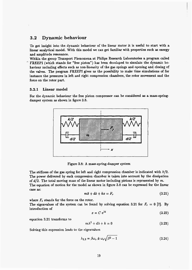
3.2 Dynamic behaviour

To get insight into the dynamic behaviour of the linear motor it is useful to start with a linear analytical model. With this model we can get familiar with properties such as energy and amplitude resonance. Within the group "ransport Phenomena at Philips Research Laboratories a program c d e d FREEPI (which stanids for "free piston") has Deen devebped io s i m d & ~ the &jiìâmic be= haviour including eitects such as non-linearity of the gas spriïìgs a d qeí i ing 2 ~ d chsiug d the valves. The program FREEPI gives us the possibility to make time simulations of for instance the pressures in left and right compression chambers, the rotor movement and the force on the rotor part.

i -

3.2.1 Linear model

For the dynamic behaviour the free piston compressor can be considered as a mass-spring- damper system as shown in figure 3.8.

I ! I !

f i i 7 - X

Figure 3.8: A mass-spring-damper system

The stiffness of the gas spring for left md right compression chamber is indicated with k/2. The power delivered by each compression chamber is taken into account by the dissipation of ú/2. The total moving mass of the linear motor including pistons is represented by m. The equation of motion for the model as shown in figure 3.8 can be expressed for the linear case as:

mx + dx + ka: = F, (3.21)

where F, stands for the force on the rotor. The eigenvalues of the system can be found by solving equation 3.21 for F, = O [7]. By introduction of

2 = c ext (3.22)

equation 3.21 transforms to mA2 + dX + k = O

Solving this expression leads to the eigenvalues

(3.23)

(3.24)

19

where wo equals the undamped eigenfrequency:

wo = \I" m

and p stands for the dimensionless damping coefficient: ..

For our system p < 1 which means that the eigenvalues can be written as

x1,2 = pwo f j w o d ( l - B2)

The imaginary part is known as the damped eigenfrequency:

(3.25)

(3*2!q

(3.27)

w; = wo\/( 1 - p 2 ) (3.28)

For the forced response solution we assume a harmonic excitation and response expressed as:

Fr = FrdWt (3.29)

2 = ie+* (3.30)

where Fr and i are complex amplitudes with a certain phase shift @ in between. Substitution of equations 3.29 and 3.30 into 3.21 yields for the amplitude ratio:

with

The phase shift equals:

W f l = - WO

Amplitude resonance

The maximum value for equation 3.31 will be reached for

(3.31)

(3.32)

w = wo\/cl- 2p2) (3.33)

This frequency which is cdled the amplitude resonance frequency will be less than the damped eigenfrequency (for p # O) as given in 3.28.

Energy resonance

We are interested in the frequency with a maximum power dissipation for a certain value of F. We call this situation energy resonance. The power dissipation is proportional to the amplitude of the velocity, so we have to find a maximum for:

20

It can be verified that this equation has a maximum for:

This means that we have energy resonance at the undamped eigenfrequency . At this fre- quency the phaseshift between force and position is 90 degrees so there is no phase shift lieixveri fûïce a d vd~cftj.. IE cther wm&, the mass ~CI-CP nzZ and aoaina z - c z force kz cancel: so the ïûtûî fsrce eqUds the damping f9rce:

F, = dx (3.35)

Within this report the term resonance Prequency is used for the energy resonance frequency. When the system is at resonance the dissipated power P equals:

(3.36)

In order to minimize friction, leackage and valve losses it is favourable to have a resonance frequency f M 50 Hz and an amplitude 5 z 9 mm 1131. According to 3.36 we find for these values and a power dissipation of P = 50 W that the force amplitude must be @, = 35.4 N. The ratio between k and m is specified by the resonance frequency according 3.25. For a resonance frequency of f = 50 Hz the following expression holds:

k m - = wo = (1007r)2 (3.37)

So with respect to the resonance frequency we can freely choose the absolute value of k or m. However the dimensionless damping B depends on the absolute value of k or m:

The sharpness of the resonance peak is strongly influenced by ,d 171. With respect to the controlability of the system we like to have a more or less flat resonance peak, or a high value of ,d which can be reached for a small value of rn and k. However the mass of the moving part m can not be choosen freely because the rotor dimensions are determined by the necessary electromagnetic force as outlined in previous paragraph. The prototype as discussed in chapter 4 has a moving mass rn = 0.837 kg. For an approximation of /3 according to expression 3.38 we have to determine d. The value of d can be obtained from 3.35:

= 0.0125Nsm-1 35.4 x 2, 1 0 0 * a * 9

According to 3.38 we find for the dimensionless damping:

= 2.28 * IO-' 0.0125 2 * 100 * K * 0.837

- d b o m

p = - -

This value results in a sharp resonance peak so an accurate frequency control is necessary. According to 3.37 the stiffness should be k = 82.6 * lo3 N/m for a moving mass m = 0.837 kg. The piston diameter must be choosen in such a way that this stiffness is reached. We have chosen for a piston diameter of 32 mm which results in the desired stiffness as shown in next paragraph.

21

Estimation stiffness k

In reality we have a non-linear stiffness due to the adiabatic compression and expansion of the gas inside the compression chambers. For an estimation of the linear stiffness IC we consider the situation that the pressure in the compression chambers just reaches the discharge pressure pd so that the outlet valves remain closed. For this case the pressure in left and right chamber $%&her with the retmlting fmce the moving pat are shmvn as a fun&m of the mtûr n-itinn in fig10 3-9- r -- ---y

o - x p

.............................. \ -2

-%?

%?

Figure 3.9: Pressure and Force on the rotor

A simple approximation for k can be made by saying:

(3.39)

Already this approximation shows that the stiffness k and so the resonance frequency depends on the discharge pressure pd and suction pressure ps which axe defined by the operating conditions of the cooling system as discussed in chapter 2. A more fundamental approximation for the stiffness k can be done by the assumption that the work on the rotor during the piston movement from x = O to x = 2 should be equal for the linear and non-linear stiffness. For the pressure in left (pi) and right (pr) chamber the following equations hold:

(3.40)

where 2 , stands for the maximum amplitude of the piston. The resulting force Fr equals :

Fr = (Pr - ~ r ) A p = psAp(2m + 2)" [ ( i m + z)-" - (2, - .)-%I (3.41)

22

For the work done during the piston movement from x = O to z = 2 the following expression can be derived for K # 1:

K-1 (3.42)

Wnonìinear = -

For the same &qIaceaezt the wc& &ne by a gue&r spriug ep2.s:

(3.43) 1 2

Wijnear = -LE2

For the assumption

we find for k : Wnoniinear = Wiinear

A

5 # O (3.44) 2ps A p 2m k =

Looking at the cooling circuit in chapter 2 we see that the discharge pressure pd and suction pressure p , are determined by the temperature of evaporator and condensor. So it is useful to express the amplitude ratio as a function of the pressure ratio. Working out expression 3.40 leads to : 1 1 -1

= [(E) ;i - 11 . [ (R) ;i + 11 2.m

(3.45)

B y substitution of the amplitude ratio found with equation 3.45 into equation 3.44 we are able to calculate the resonance frequency as a function of the discharge and suction pressure. For a moving mass of 837 gram and a piston diameter of 32 mm this leads to the characteristic shown in figure 3.10.

3.2.2 Non-linear model

The dynamic behavieiir including non-hear effects can be estimated with the computes pro- gram FREEPI. A detailed description of this program can be found in [9]. The user input for the motor part consists of the static force characteristics, the electric loss characteristics, the self-inductance and the resistance of the coil. Besides these values other parameters such as piston diameter and maximum amplitude have to be given. A complete list of input parame- ters can be found in appendix F where an example of a freepi run is given. It is also possible to take into account leakage between piston and cylinder and friction losses. A parameter investigation can be done easily by setting a lower and iipper value and number of iterations for the desired parameter. Calculations with FREEPI show that the mean position of the rotor drifts away from the mid- position if no precautions are taken. This drift phenomena can be explained by looking at the resulting force on the rotor part over one period. The pressures in left and right chamber (PI and pr) as a function of the rotor position are shown in figure 3.11 for a prescribed sinusoidal movement. The solid lines indicate the pressures for a movement around the midposition and the dashed lines for a movement around an eccentric position 2,. B y integration of the force on the rotor over one period for different eccentric positions zo a characteristic as shown in figure 3.12 can be obtained. From this characteristic can be concluded that for a small displacement of the mean rotor position a resulting force will occur in the same direction.

23

50

40

30

Suction Pressure Ibaral

-

-

I I I

pr-1.0

+ pr-1.2

+#- pa-1.4

f3- p a 4 6

++ pr-1.8

4 pr-2.0

_c

Figure 3.10: Resonance frequency as a function of suction and discharge pressure calculated with linear model

In other words: the midposition is an unstable equilibrium. Due to this drift phenomena one cylinder will act as a gasspring and the other as a pumping cylinder. A reduction of the drift can be reached by the use of trigger holes and/or buffers. These options are shown in figure 3.13. The trigger holes take care that for both chambers the compression starts with the same compression volume resulting in a more symmetric load of the rotor over one period. The ap- plication of buffers results in an extra gasspring for a certain amplitude of the rotor. Besides a reduction of the drift this option also prevents that the pistons hit the valve plates.

24

pd . . . . . . .

ps ......

._._____........ <......... - ....... /-l.; 1 i u- *.*** -

...... .-' f.

*.- .. ... e... e..

... '.. ..

Centric movement

Eccentric movement

Figure 3.11: Pressures in left and right chamber

Figure 3.12: Resulting force on rotor as a function of the eccentric position x,

25

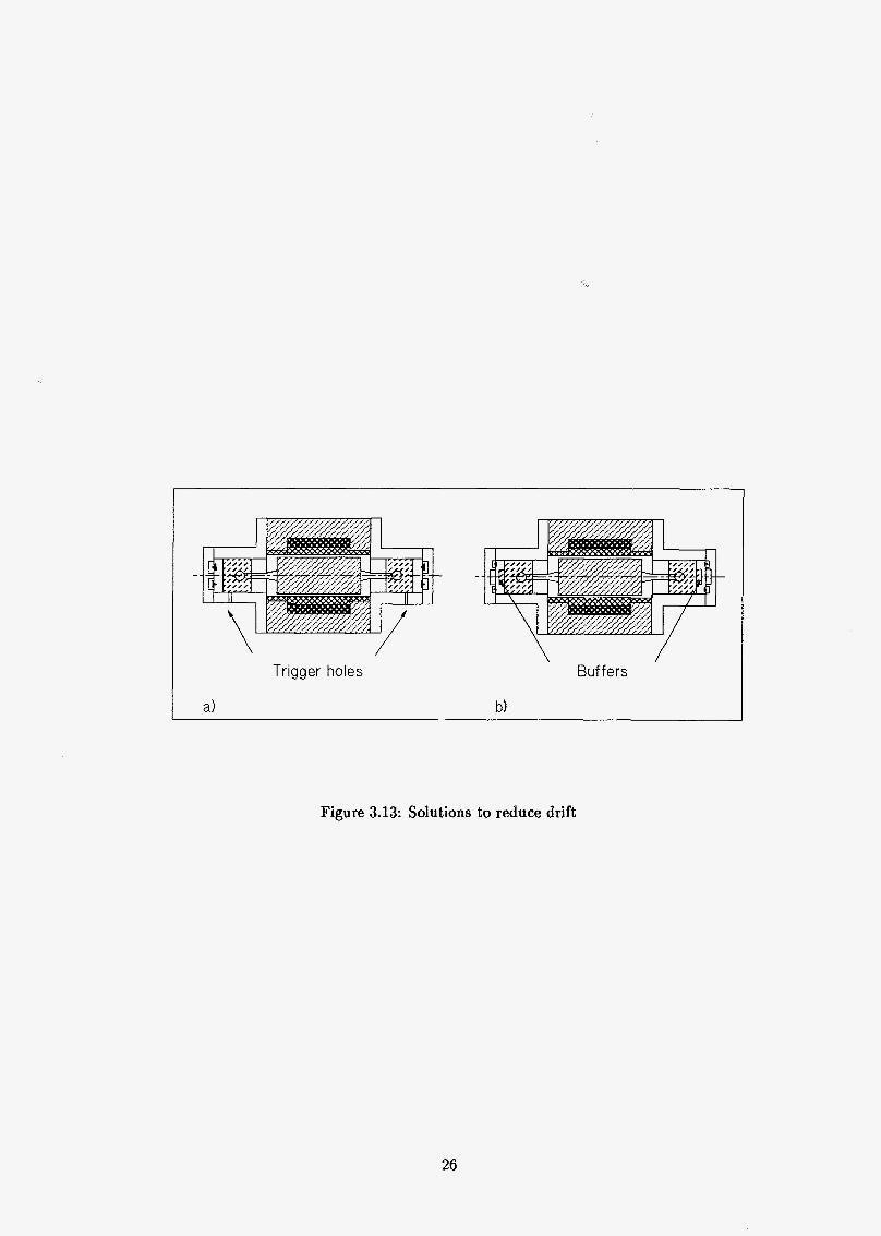
-1 a)

Trigger holes

b)

Buffers

Figure 3.13: Solutions to reduce drift

26

3.3 Electric Circuit

For the analytical as well as the finite element model all the calculations have been done with a prescribed number of ampere turns N i . In fact a current density is prescribed at the coil area. Up to now no distinction is made if this density is reached for a large number of windings and a small current or the other way around. The number of windings is restricted by the avaiiabie supply VQItage and the uecessary ûütpt pmw 05 the uicter. Fm a g o ~ d aesign oÎ the co2 with these boüudaiy cûiiditiû~s the se!EnU~c$mce ef the n ~ t ~ r neecl to he known. The inductance can be calculated with the analytical model of the magnetic circuit. A more accurate prediction can be made with the finite element model.

. .

3.3.1 Inductance of motor

For a coil the following expression holds according to Faraday’s law:

From this expression the following equation for the inductance L can be obtained:

dqì L = N- di

(3.46)

(3.47)

For the magnetic circuit analysis the magnetic flux 4 is calculated as a function of N i so it is more convenient to express the inductance as:

We call CL the coefficient of inductance which caa be expressed as:

& CL = - d N i

(3.48)

(3.49)

For the design of the coil we consider the inductance at the midposition (z = O). The nqpe t i c reluctace RI + R, has a minimum at this position (see equation 3.9) resulting in a maximum value for the inductance. The coefficient of inductance CL can be calculated by means of the analytical and finite element model of the magnetic circuit.

Analytical model

An approximation of CL can be done with the aid of the magnetic circuit shown in figure 3.3. When the rotor is in this position (z = O) the magnetic resistance of left and right circuit are equal so RI = R, = RI,. For this case the flux generated by the coil equals:

(3.50)

The coefficient of inductance can be found by substitution of this equation into equation 3.49 resulting in:

1

(3.51)

Working out this expression for the dimensions given in paragraph 3.1.1 leads to CL =1.5*10-7 [HI for the corovac motor and ch=2.8*lV7 [RI for the iron motor.

27

Finite element model

A better approximation of the inductance can be made by the PE2D finite element model. For the determination of CL we replace the permanent magnets by air gaps which has not much influence on the inductance because only the magnetic flux caused by the coil play a part for the inductance of the motor. The property CL can be approximated now by taking a s r n d value of Ni and calculate the corresponding flux d. This resulted in ~ ~ = 3 . 3 * 1 0 - ~ [Hl for the corovac motor and c ~ = 4 . 3 * 1 0 - ~ [HI for the iron motor. So for a coil with 1175 windings the predicted inductance L = 11752 * 3.3 * lo-' = 45ömH for the corovac motor. Comparing these values with the values of the analytical model we see a great difference which is caused by the stray flux which is not taken into account within the analytical model. The stray flux results in an increase of the total flux 4 compared to the analytical model.

3.3.2 Coil design

Number of windings

The number of windings can be determined if the following quantities of the motor are known:

1. maximum rms value of the supply voltage U

2. maximum total power dissipation Pt

3. coefficient of self inductance CL

4. running frequency w

5. number of ampere turns Ni needed to reach the maximum power dissipation Pt.

When the system is at resonance the electric scheme reduces to the one shown in figure 3.14

lm

Figure 3.14: Electric scheme for system at resonance

The totai power dissipation Pt consisting of mechanical power, copper losses, hysteresis losses

28

and friction losses is represented expressed as:

For the supply voltage amplitude

by the power dissipation of resistance Rt, so Rt can be

Pt Rt = - i 2

(3.52)

(3.53)

For a sinusoidal current and voltage the following expressions hold for the rms values U and a :

This means that equation 3.53 can also be written as:

U Z = ( ~ w L ) ~ + (iRt)' (3.55)

Substitution of equations 3.52 and 3.48 results in

U Z = N 2 [WCLNi]2+ - ( (3.56)

Rewriting equation 3.56 leads finally to an explicit expression for the number of windings.

U N =

J(iWCLNi12 + [%I2) (3.57)

The number of windings has to be chosen in such a way that for a given maximum supply voltage the maximum power dissipation can be reached. In figure 3.15 the number of wind- ings as a function of Ni is plotted for different values of the selhductance constant c ~ . The chosen values for the other variables are:

Pt = 85 [Wl w = íOO?r rad.^-^] u = 20c [VI

Take care, N i stands for the rms value and not the amplitude. The force characteristics obained in the first paragraph of this chapter show that the max- imum delivered power of the motor will be 70 W for N i = 1200 (Ni = 1700). The total electric losses are approximately 15 W resulting in a total power dissipation of Pt = 85 W. In previous paragraph we have shown that c~ = 3.3 t H for the corovac motor. From figure 3.15 can be read that the number of windings should be approximately 1300.

Diameter of wire

Before we are able to fix the diameter of the wire we have to know the coil space factor f w which is defined as the ratio between copper area and to td coil area. The maximum theoretical space factor for a coil wound as shown in figure 3.16 can be expressed by usage of the definition for the indicated triangle :

(3.58)

29

" O 600 1000 1600 2000 2600 3000 3600

N*i [A]

CI-lo-7 -I- CI-Ze-7 ?y- CI.3.-7

-8 CW.-7 * c c m - 7

Figure 3.15: Number of windings and cos4 as a function of N i

Figure 3.16: Maximum coil space factor

So for a wire with do = 0.75mm and d; = 0.7mm we find a maximum value fw = 0.79 . In practice a value of approximate f w x 0.74 can be reached. For the coil of our model as shown in figure 3.2 the space factor can be defined as:

N?r4 f w = - 41,b;

So the diameter of the wire can be expressed as:

(3.59)

(3.60)

3.3.3 Elec t r i c power losses

The electric power losses can be subdivided in static losses and dynamic losses. The static losses or copper losses are due to the electric resistance of the coil. The dynamic losses are the frequency dependent losses and can be subdivided into hysteresis losses and eddy current losses.

30

Stat ic losses

The resistance of the coil can be expressed as:

(3.61)

--l. --- wuclt : Dc sta;;& fûr the u~erzge r d &meter aad Aw for the cross sectional wea ûf the win&.ng. r, copper wire with a &meter of di we can rewrite this expression to:

The resistance losses or copper losses of the coil can be expressed as:

pcopper = i2Rc

For a prescribed current density J it is more convenient to use next expression:

(3.62)

(3.63)

in which V, represents the volume of the coil. For our model the current density is defined as:

(3.65)

Care must be taken to take the right resistivity for copper because this value is temperature dependent. At normal operation the temperature of the motor will be approximately 80 "C. The increase of the resistivity can be calculated by next expression:

dP - = adT P

(3.66)

where a is called the temperature coefficient. For copper a=0.0043 K-' and pe = 17.10-' R m at room temperature (20 "C). According to expression 3.66 the resistivity for copper at 80 "C can be found in the following way:

In(Pe800C) - In(pe20~) = 60 * a

In(pemoc) - ln(17.10-') = 60 * 0.0043 + pemC = 2 2 . 1 0 - ~ ~ m

For the dimensions of the coil for our motor as given in paragraph 3.1 we find for Ni = 1200 (Ni = 1700):

Dynamic losses

The dynamic losses consist of hysteresis losses and eddy current losses as discussed in [li].

Pdyn = p h y s t Peddy

The hysteresis are caused by an alternating magnetic flux through a ferromagnetic material. A typical hysteresis loop of an arbitrary ferromagnetic material is shown in figure 3.17. The

31

I

Figure 3.17: Hysteresis loop of a ferromagnetic material

enclosed area of the hysteresis loop is a measure for the hysteresis losses over one period in flux change. This means that the hysteresis losses are proportional to the frequency so we can write:

Phys = C i f

where the factor c1 depends on the alternating flux density, the hysteresis loop of the ferro- magnetic material and the volume of the material. For soft iron an alternating fiux density of 1 T at 50 Hz the hysteresis losses will be approximately 1 W/kg [li]. For corovac under the same circumstances this value is about 8 W/kg. The eddy current losses are a result of the induced voltage due to an alternating magnetic flux according to Faraday’s law. The induced voltage is proportional to the frequency of the magnetic flux change and the eddy current losses are proportional to the induced voltage to the square. Thus we can approxhate the eddy current losses by:

where c2 depends on the electric resistivity of the conductive material and the alternating magnetic flux. For corovac the eddy currents are neglectable due to very high electric re- sistivity P e x 1.5Qm (for unlaminated iron Pe w 10-7Rm ). This is also confirmed by the experiments discussed in chapter 5.

32

Chapter 4

ealisation of prototy

We have build two prototypes to investigate the behaviour of the linear motor. One prototype has been build from iron (UN-N925) and the other from corovac (EF6060). The iron motor was build to get an indication of the behaviour of a laminated iron motor which will probably be build in the near future. The dimensions of the prototypes are as given in chapter 3.1.1 except for the iron motor the height of the outer magnet I,, = 2mm. Figure 4.1 shows the components of the linear motor.

Figure 4.1: Components of linear motor

3 3

4.1 Soft magnetic material

An alternating magnetic flux will induce an electric field strength according to Faraday’s law. Unfortunately most materials with a good magnetic conductivity have also a good electric conductivity which means that an alternating magnetic flux results in an electric current. To reduce this electric or eddy currents some precautions can be taken. TL.. ut: --n

nûrmdly !&y i= the rmge ef 0.35 to !M.li mm. Lamination should be perpendicular to the eddy currents or parallel to the fluxlines. For most applications, such as lamination of a transformer, this leads to a simple manufacturing process. However in our model eddy currents tend to go in circumferential direction so lamination should be done somehow as shown in figure 4.2. At first instance we have chosen to prevent eddy currents by the use of a

widdy nsed m e f h ~ d is the ~ s e ef Zixniinnted iron. Thc thiekaess of t h s e Iamioates

electric isolation

iron

Figure 4.2: Lamination of cylindrical parts

material called corovac . This material consists of small particles from soft magnetic material who are electrically isolated from one another. A disadvantage of this material is the low permeability (pr z 200) compared to iron (pr z 2000). Although the permeability differs a factor i0 the generated electromagnetic force is only 27 % lower for corovac compared to iron for the same dimensions (see figure 3.7). Measurements of the B-H curve on some samples of coroviu: as used in our motor show that the magnetic properties do not meet the specifications of the manufacturer. The measured permeability differs between /Jq- = 100 and pT = 20. So the permeability is much too low and inhomogeneous resulting in a decrease of the generated force. It seems that the manufacturer of corovac has problems with the fabrication process which are not solved in the near future. For this reason it is worth-while investigating the application of laminated iron in the near future. Besides the higher permeability this material has the advantage that the magnetic properties are homogeneous. A disadvantage is the way of lamination that must be done somehow as shown in figure 4.2 which looks rather difficult for mass-production. Suggestions for a simple fabrication process are welcome !

4.2 Permanent magnets

For the permanent magnets we have chosen for FXD330 [i] which is cheap and commercially available. Permanent magnets made from this material have a magnetic orientation obtained during the manufacturing process. As far as we know, ferroxdure rings with a magnetic radial

34

orientation are not commercially available. This problem is solved by shown in figure 4.3.

using 4 segments as

Magnetic orientation

Figure 4.3: Magnetic ring made from 4 segments

The magnetic orientation is not pure radial resulting in a reduction of the effective radial coercivity. An estimation for the effective coercitivety can be made by integration of the radial component:

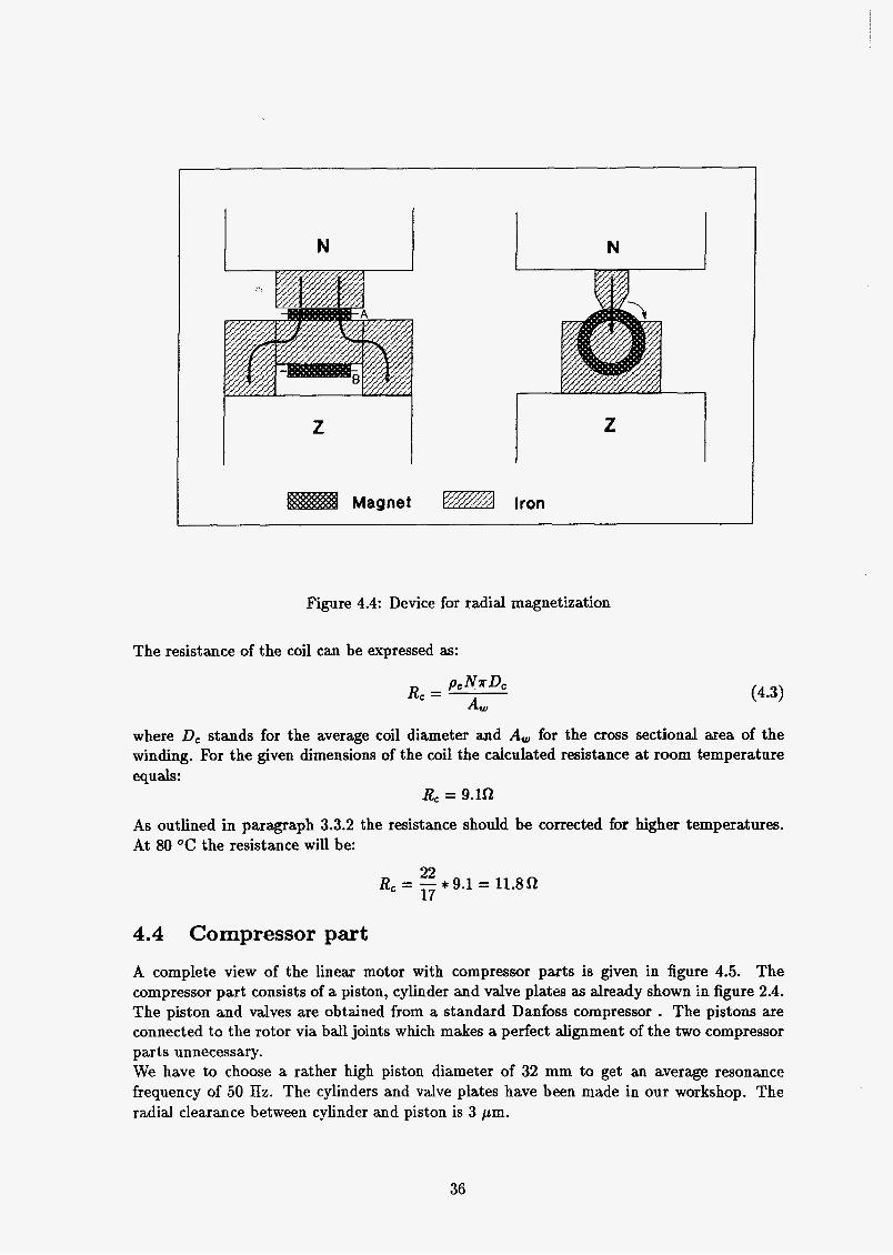
The analytical and ñnite element calculations discussed in previous chapter are obtained with this correction. Permanent magnets are normally magnetized in an axial magnetic field. Radial magnetization in an axial field cm be done by the use of a device as shown in figure 4.4. The field strength of the magnetizer must be chosen in such a way that the needed flux density for full magnetization (at least 1.2 T) will be reached at line A. On the other hand the field strength must not be chosen too high because the complete flux must be discharged, as indicated with the solid arrows, to prevent demagnetization at line B. Once the magnetizer Bas been tuned in such a way that these requirements are fulfilled the magnetic ring can be magnetized by turning it over 360 degrees in the direction as indicated with the dashed arrow. A patent application has been written for this way of radial magnetization which is in particular attractive for magnets made from rare-earth materials such as NdFeB and SmCo.

4.3 Coil

For the design of the coil we have to determine the number of windings and wire diameter as outlined in paragraph 3.3.2. As shown in figure 3.15 we have to choose the number of windings N sz 1300 for the corovac motor with a coefficient of inductance CL = 3.3 $

We did not make a separate coil for the iron motor because this motor will only be used for static measurements. Usage of expression 3.60 gives for the diameter of the wire d; = 0.70 mm. We have chosen for the available copper wire diameter with d; = 0.71 mm and do = 0.76 mm. The realised coil has an inner- and outer diameter of 49 and 66 mm respectively and a length of 75 mm. The reached number of windings N = 1175 resulting in a filling factor of:

Nnd2 41,b;

1175 $ n * 0.712 4 * 8.5 * 75 fw=--- - = 0.73

35

N N

Figure 4.4: Device for radial magnetization

The resistance of the coil can be expressed as:

where D, stands for the average coil diameter and A, for the cross sectional area of the winding. For the given dimensions of the coil the calculated resistance at room temperature equals:

R, = 9x-2

As outlined in paragraph 3.3.2 the resistance should be corrected for higher temperatures. At 80 "C the resistance will be:

4.4 Compressor part

A complete view of the linear motor with compressor parts is given in figure 4.5. The compressor part consists of a piston, cylinder and valve plates as already shown in figure 2.4. The piston and valves are obtained from a standard Danfoss compressor . The pistons are connected to the rotor via ball joints which makes a perfect alignment of the two compressor parts unnecessary. We have to choose a rather high piston diameter of 32 mm to get an average resonance frequency of 50 Hz. The cylinders and valve plates have been made in our workshop. The radial clearance between cylinder and piston is 3 pm.

36

Figure 4.5: Linear motor with compressor parts

37

Chapter 5

Experiments

5.1 Magnetic flux density The radial magnetic flux density has been measured inside the stator without rotor. The flux density is inhomogeneous in circumferential direction due to the fact that the magnetic rings are composed of 4 segments. The measurements have been carried out by mounting the stator in a turning lathe and a hall sensor on a slider. The hall sensor is slowly moved in axial direction during rotation of the stator. The signal coming from the h d sensor is filtered by a low-pass filter to get an average value of the magnetic flux density. The measured and calculated magnetic flux density are in good agreement as can be seen in figure 5.1. The measured peak at the mid position is caused by the fact that the inner magnet consists of two separate rings.

-

cakulatsd ---. measued - 0.15 I I I I 0.10

0.05

0.00

-0.05

-0.1 o

-0.1 5 -80 -40 O 40 80

Axial paition hnl

Figure 5.1: Magnetie flux density distribution

5.2 Force characteristics

For the measurement of the static force characteristics an experimental set-up has been build as shown in figure 5.2. The air-bearings are used to ensure a frictionless movement of the

38

Force Transducer

Air bearing

3-

/ Spindle

Figure 5.2: Experimental set-up for static force measurement

rotor and to prevent stick-slip problems. Each of the air-bearings can be aligned in two directions which makes it possible to position the rotor centric with respect to the stator. The rotor can be k e d at every position within the stroke by means of two spindles. The force characteristics are obtained by measuring the force for every mm displacement at 4 different DC current levels: O, 500, 1000 and 1700 ampere turns. The characteristics for 500,1000 and 1700 ampere turns are only measured around the midposition to prevent demagnetization as outlined in paragraph 3.1.2. The measured characteristics for the corovac and iron motor are shown in figure 5.3 together with the characteristics obtained with the finite element model.

.We have already mentioned in*previous chapter that the magnetic properties of corovac do not meet the specification given by the manufacturer. The measured permeability varies between pr = 100 and pr = 20. The calculated characteristics as shown in figore 5.3a are carried oat with the measured curve Q€ pp = 100 as input. The difference between measured and calculated force for the corovac motor is within 3% at the midposition. The slope of the measured curve is higher which indicates that the permeability is lower in reality as assumed (the slope of the force characteristics or the reluctance force depends on the permeability as already shown with the analytical model in figure C.7). For the iron motor the correlation between calculated and measured curves is not so good in absolute value although the slope of the curves (or reluctance force) corresponds very well. Due to the good agreement in reluctance force it seems that the magnetic properties of iron are in good agreement with the B-H curve used as input for the finite element calculation. Unfortunately we have no good explanation at this moment for the difference in absolute value.

5.3 Electric losses

The electric losses P, are measured by fixing the rotor in the midposition. The fixed rotor ensures that no energy is dissipated as mechanical energy like friction losses. The measure-

39

9-8-7-6-6-4-3-2-1 O i 2 3 4 O 6 7 8 0

Rotor position (mm)

a) Comvac motor

Mmo Fr (N)

1 2 0 1

-lo -6 O 6 lo

Rotor position x (mm)

b) Imn motar

Figure 5.3: Force characteristics

ments have been carried out by supplying the coil with a current of constant amplitude and varying the frequency step by step. This procedure has been carried out for several values of the current. For ewh current i and frequency f the supply voltage U and input power Pe (which equal the electric losses for a ñxed rotor) are measured. Figure 5.4 shows the measured electric losses E!, as a function of the frequency for the corovac motor. We have shown in paragraph 3.3.3 that the electric power losses can be subdivided in static -losses (or copper losses) and dynamic €osSeS. The dynamic losses are the frequency dependent losses which can be subdivided into hysteresis losses and eddy current losses. Extrapolation of the measured curves of figure 5.4a to zero frequency gives the copper losses. The values obtained in this way differ brom the expected values according to

for the measured resistance of the coil R, = 9.40. This differeke c m be explained by the temperature rise of the coil during the measurement which results in zan increase of the coil resistance as discussed in paragraph 3.3.3. The dynamic losses can be easily obtained by subtracting the extrapolated losses at zero frequency from the measured total losses:

Pdyn = pe - P q p w

We have shown in paragraph 3.3.3 that the dynamic losses consist of hysteresis losses and eddy current losses according to:

In genera3 it is difficult to make a distinction between hysteresis losses and eddy current losses from the measurements because c1 and c2 are dependent on each other. This is due to the

Total &.ctrio b u o . Po (W)

l8 1

o 2 4LL O 20 40 60 80 100

f [Hzl

1-0.26 A b0.6 A -#+ i-0.76 A -8 1-1.0 A

a) Total electric losses

i

0.02 1

I - - 4,

o ’ I 1 I

O 20 40 60 80 100

f IHzl

- 1-0.25 A -4- i-0.6 A -#+ 1.0.76 A -8 14.0 A

Figure 5 .4 Electric losses

fact that the eddy currents reduce the magnetic flux resulting in a reduction of the hysteresis losses. The best way to make a distinction is to plot the curve:

-- Pdyn - c1 + cz f f

The slope of the curve ives an indication of the eddy currents losses whereas the extrapolated value of the function at f x = O gives an indication of the hysteresis losses. With this definition we can conclude from figure 5.4b that the dynamic losses consist mainly of hysteresis losses. The mea;surement of B., U, t md 4 enables CS to cdcdate the inductance L and cos q5 of the motor. The electric scheme shown in figure 3.14 can be used to obtain the following relations.

$à n

w

pe cos4 = - U i

The values for L and cos 4 obtained in this way are shown in figure 5.5. The inductance of the motor is hardly influenced by the frequency and the current. The average value of 380 mM is smder then the predicted value of 456 mH by the finite element calculation in paragraph 3.3. This indicates that the average magnetic permeability of corovac is smaller as assumed for the finite element calculations which corresponds with the conclusion given at the evaluation of the force characteristics in previous paragraph. The insensitivity of the inductance for the current results as expected also in an insensitivity of cos 4 for the value of the current. During operation of the motor the value of cos 4 will be higher due the mechanical power consumption which results in a higher real part of the supply voltage as shown in figure 3.14.

4:

Inductance (mH)

0.2

0.1

600

400

300

200

1 O0

O

-

-

d

8 I I I I

Codphi)

O*=*

nl I I I I I I , - O 10 20 30 40 60 80 70 80 O 10 20 30 40 60 60 70 80

f IHzl f IHzl

A I.0.2I A k0.6 A i-0.75 A -8 1-10 A - 1-0.26 A -f- 1-0.6 A bO.76 A 8- b1.0 A

Figure 5.5: Inductance and cos 4

5.4 Efficiency

The efficiency of a motor is defined as the ratio between the power delivered by the rotor and the power consumption of the motor. For the delivered power by the rotor the following expression holds:

(5.1) 1 - - 1 - 2 2

Pr = FT2 = -FrX = -wF~Z

The total power consumption of the motor equals the delivered power by the rotor plus the electric losses. The eficiency bos merent number of ampere turns as shown in next table is obtained from the measurents shown in figure 5.3a and figure 5.4a. A resonance frequency of 50 Hz and an amplitude 2 = 9 mm is assumed.

Interpolation of the values of this table shows that q = 87 % for Pr = 50 W. When the material properties are as specified by the manufacturer the efficiency will increase to q R 90 % So we can make the conclusion that the goal of T,I = 90 % for P,. = 50 W is possible for a motor with corovac as specified by the manufacturer.

4%

Chapter 6

Conclusions and remarks

The feasibility of a free piston compressor with an integrated linear motor has been in- vestigated. The following remarks and conclusions can be drawn from the theoretical and experimental analysis:

o A free piston compressor with an integrated linear motor as proposed in this report is constructively very attractive, it contains less parts and the manufacturing process is simple.

o The radial forces are almost eliminated by the use of large air gaps between rotor-ends and stator. The generated electromagnetic force can be increased with 40% by filling these air gaps with permanent magnetic material. There exists an optimum for the thickness of these permanent magnetic rings.

o The analytical model of the magnetic circuit proved to be a useful tool to investigate the influence of the design parameters. The results obtained with this model corre- spond qualitatively well with the results of the finite element model. However, the predicted electro magnetic force with the analytical model is 30 % higher compared to the ñnite element model. This is caused by the stray flux and non-linear behaviour of the magnetic material which are not taken into account within the analytical model

o The magnetic properties of eorovac do not meet the specifications given by the manufac- turer. The measured B-H curves on some samples of corovac show that the magnetic permeability is much to low and inhomogeneous. The measured permeability varies between pr = 100 and pr = 20. This causes a reduction of the generated electromag- netic force with approximately 15 %. Due to these problems it may be worth-while to investigate the application of laminated iron.

o Although the magnetic properties of corovac do not meet the specifications a motor motor efficiency of 87 96 can be reached for an output power of 50 W. If the magnetic properties are according the specifications the efficiency will be approximately 90 %.

o At this moment the prototype is built in a calorimeter set-up. From the measurements taken up till now we can conclude that the radial forces are low. The measured mean resonance frequency corresponds with the predicted value of 50 Hz. The measurements are in a too early stage to make conclusions with respect to the overall efficiency and cooling capacity.

43

Bibliography -

[i] Data handbook pennanent magnet materials C1ö. Philips, components and materials,

[2] Version 8.2. THE PE2D REFERENCE MANUAL Vector Fields Limited, 24 Bankside,

[3] F.A. BOOR. A compressor motor with permanent magnet rotor. Master’s thesis, Eind-

[4] F.A. Boon and G.C. Goverde. Analysis of a f i e piston compmssor system. Technical

1986.

Kidlington, Oxford OX5 IJE, England, 1990.

hoven University of Technology) 1988.

Note 248/86, Nat.Lab, 1986.

[5] Anthony C. Hearn. REDUCE USER’S MANUAL. The Rand Corporation, Santa Mon- ica, CA 90406-2138, 1987.

[6] M.J.P. Janssen. Cycling losses in cooling circuits. Master’s thesis, Eindhoven University of Technology, 1989.

[7] Erwin Kramer. Maschinendynamik. Springer-Verlag, 1984.

[8] L.J.M. Kuijpers and R.C.D. Lissenburg. Some remarks on continuously contmlled wm- pressors. Technical Note 257/86, Nat.Lab, 1986.

[9] R.C.D. Lissenburg and P.J.M. Verboven. F’pi: a computer simulation pmgmm of the free piston compressor for freezer and refrigemtor cooling cycles. Technical note 135/86, Phillips Research Eindhoven, 1986.

[lo] Edward J. Finn Marcello Alonso. Fundamentele Natuurkunde, deel 2 Elektmmugnetisme. Delta Press BV, Overberg, The Netherlands, 1988.

[ll] R.H. Munnig Schmidt, J.H.M. Hensing, and J.J. van Herk. The application of moving coil linear motors in wipmuting compressors. Report 5916, Nat.Lab, 1984.

[12] J.A. Schot. Aandrijvingen, elektromechanische basisstof en inleiding tot de elektmmech- anische energie-omzetting. Dikta t 5656, University of Technology Eindhoven, 1985.

[13] P.J.M. Verboven and P.H.S. Westerhoven. Evcrluatioon dof the hybrid electmmotor for refigemtor compressors. Technical Note 327/87, Nat.Lab, 1985.

44

Appendix - A I?

Derivation of electromagnetic force

A first approximation of the magnetic behaviour can be performed in an easy way by the introduction of the concept of magnetic potential and magnetic resistance. With this concept magnetic circuit analysis can be treated in the same way as for an electric circuit. For a linear analytical analysis the following assumptions have to be made:

o linear behaviour of magnetic material

o no saturation

e no stray flux

Although these assumptions will result in a considerable error we have the experience that an analysis done in this way gives good insight into the magnetic behaviour qualitatively. In general we can say that for the magnetic behaviour an electric motor can be divided into the following parts:

o coil and/or permanent magnets which are the sources for the magnetic flux.

e air gaps and magnetic conductors like iron which form the resistance for the magnetic flux.

The mapetic p ~ t m t i d generated by a coil with N windings and a current i can be expressed by (see [12]):

U , = N * i ( A 4 For an ideal permanent magnet with a relative permeability /Ar = 1 and a homogeneous magnetization in direction 1, the magnetic potential is defìned as:

For a magnetic conductor with a relative permeability the magnetic resistance or reluctance R, is defined as:

For an air gap the relative permeability pr = 1 so A.3 reduces to:

45

I Ni I

I I I

b-x -. ._.__. L.4 ._.. 3.

Rot or \

Figure A.1: Model of a reluctance motor with electric scheme

For the derivation of the generated force of a linear motor we use a simple model as shown in figure A.1. The rotor can only translate in direction. The magnetic resistance of the iron parts is considered to be independent of the rotor position 2, only the resistance of the air gap is taken as a function of z. Utilisation of the rules given in equations A.l to A.4 leads to the following expressions for magnetic potential, resistances and flux :

Um = N i (A.5)

Where d stands for the length of the model in the third dimension and 2, for the mean iron length of rotor and stator.

By using Faraday's law we can express the supply voltage for the coil with resistance R, as:

@ U = i& + N- dt The electric energy supplied in a time period dt to the coil diminished by the energy dissipated in resistance Rc equals:

As described in reference [12] the supplied energy diminished by the dissipated energy in resistance Pe, is transformed to magnetic field energy wid mechanical work according to the

Uidt - Rci2dt = N i d 4 (A.9)

46

relation: Uidt = N i d 4 = dWm + Fed% (A.lO)

where dWm and Fedx stands for the magnetic field energy and mechanical work respectively. Fe represents the generated electromagnetic force.

From the three variables 44 and x only 2 can be chosen independent. The third one is a ~ U C ~ ~ Q O ef the other two. We choose i and x as independent variables so:

R.

Substitution of equations A.l l and A.12 in equation A.10 yields:

By introduction of the so called caenergy :

WA = N i 4 - W m

(A.12)

(A.13)

(A.14)

and the fact that equation A.13 must be valid for arbitrary values of di and úx results in the expressions:

and @WA N 4 = - ai

(A.15)

(A.16)

Suppose the rotor is fixed at a certain position x . An increase of the current from i = O to i = i e gives for the co-energy:

W& = J,” N4di (A.17)

Substitution of equations A.5 and A.7 leads to:

With equation A.14 it is easy to see that

wrn=w;=-- W?7b (A.19)

The expression for the electromagnetic force Fe can be found by substitution of equation A.18 2

into equation A.15.

I (A.20)

The magnetic flux 4 can also be expressed as a function of the inductance L of the motor:

Li 4 = - N

so the electromagnetic force can also be expressed as :

(A.21)

1.2dL Fe = -a - 2 dx (A.22)

47

It can be verified that for a circuit with n magnetic potentials Umj the superposition principle holds, so the total electromagnetic force satisfies:

with j being the sonzce zamber with SEX q+ a 4 magnetic pieniiai Notice $hat the

Equation A.23 together with the definitions for magnetic potential and magnetic flux as given in equations A.l to A.4 form the basic set of equations for the an- alytical analysis of the magnetic behaviour. Substitution of equations A.5,A.6 and A.7 into equation A.20 finally results in the following expression for the electromagnetic force on the rotor of the model shown in figure A.l:

sotu;eé cm be eûg a xd & pr7n,mpn, mw-et,

with

The optimd gap height Zgqt c m be found by means of expression

-- - O ûa

which results in:

(A.24)

(A.25)

(A.26)

So for the midposition we find:

This means that for s m d values of z/b the air gap 2, should not be chosen as smaU as possible for materials with a low relative permeability rc/r- By substitution of igw inia equation k.6 we this value corresponds with:

So with respect to the electromagnetic force the magnetic resistance of the air gaps should be chosen equal to the magnetic resistance of the iron parts.

4 = R g

Appendix B

Maxwell equations

Law Integral form Differential form

1. Gauss law for electric field j D - e N d S = q d i v D = p

2. Gauss law for magnetic field { B - e N d S = O d i v B = O

3. Faraday’s law

4. Maxwell’s law

Interactions between D and E and between H and B are described by the following expres- sions:

D = EE

B = p H

with

49

Appendix C

Force characteristics obtained with analytical model

The equation for the generated force on the rotor (3.11) obtained with the analytical model has been implemented in LOTUS in such a way that a parameter study can be done in an easy way. For dl the characteristics shown in this appendix the following nominal dimensions and material properties apply (see fig 3.2 for the meaning of the variables):

rr = 17.8 mm 1, = 9 3 mm mm b; =75 mm I,; = 6

bo = 18 mm I,, = 4 mm I, = 9 mm I, = 12 mm

mm g = 0.4 mm 2 = o

Br ~ 0 . 3 3 5 T N i = 1700

All the characteristics are shown for pr = 200 and pr = 2000 which are the assumed values for the permeability of corovac and iron respectively.

The Characteristics shorn ir; this appendk we:

Figure c . 1 c .2 c .3 c . 4 c . 5 C.6 (2.7 C.8 c .9 c.10

50

Figure C.l

20

Figure C2

-

I t I ,

Fome Fr (NI

140)

O 6

:~~ , , , ,

O 1 2 3 4

Height Imo (mm)

- with magnet

+ with magnet

+ without magnet

-8 without magnet

Figure C.3

Force Fr (NI 120

100 -

80 -

60 -

O 10 20 40

WQtQr diameter dr ámm)

z ur.200 + ur-2000

60

Forco Fr (N)

l S O 1

Gap height g (mm)

Figure C.4

Figure C.6

140)

Figure C.6

Force Fr íN)

200

I 160 -

100 -

60 -

I I , 4

OJ O 1 2 3

Number of ampereturns Ni (A) (Thousands)

up200 +ur=2000 -

Figure C.7

Force Fr (Nl I I

40[ 20

10 O -10 -6 O b

Rotor position x (mm)

Fomo Fr íN]

loo^ I 8ot1 F

I I I

O 6 10 16 20 Height iron ly (mm)

-up200 +w-2000

Figure C.8

:I 20

O 1 o 2 4 8 8 1 0 1 2 1 4

Height coil cc Cmm)

ur-200 + ur=2000 - - up200 + ur-2000

52

1 O0

50

O O

Figure C.9

~ I C O Fr (NI

10 20 30 40 60

Width outer-part bo (mm)

- ur-200 +ur=2000

Figure C.K)

FOICO Fr (H)

140

100 -

60 -

60 -

40 -

2ofi n ". O 20 40 60 80 100 120 140 160

Width inner-part bi (mm)

- ur-200 + ur-2000

53

PEZD input file

54

ui ui

inputfilm for linmar motor

/ / 1 Miin Dimmniions / / with linear motor" I for maning of vui.blmm / oonm +»r 35.6 ooni +Bi 75 oonm +Bo 10 ooni Cia, 4 aonm (slmi 6 ooni ,410 9 ooni +ly 12 aoni +g 0.4 oon. +x o ooni h i 1000 / l-ngth o f air around motor: OM. 11 20 / pmrmesbility of iron for finmar <wloulationmr ooni +p*m 200 I ooni +iip O aoni #mu0 4*3.14m-7

/ tlunmntdistribution

aona +nx6 5 loon. h u 7 4 I oonm )nyl 4 loonm b y 2 +Bol2 loonm +ny3 (Bo12 loon. b y 4 2älooni +ny5 +B0/21 aoni h y 6 +B0/2 loon. h Y 7 4 I I

mmm rmport "A fmmiibility itudy on a frmm pimtan oompraimor

I : oonm h x l 10 loon. +nx2 5 loonm #& 4looni inx4 Ilaoni +d Si

I 1 Diviiion into rmgioni I / regio 1 t/m 'i d r a w ibip-h mrta-0 p n r l x12-O x34-+Dr/Z yl4--+Bil2-+Bo-+ll y23-y14t+ll nl-+nyl 02-4-1 1 1- f4-v bZm.97 b b . 0 3 d r a w y14--tBi/Z-+Bo y23-y14t+Bo/Z-+x nl-+nyZ-#x f4-n0 d r a w uta-3 i 1 ~ 1 i i g l n pmnrbmrni yll--(#Bi+#Bo)/Z-#x y23*-#Bi/Z nl-+ny3t#x draw yl4--+Bi/2 y23--yl4 nl-+ny4 d r m w yl4-+ûi/2 y23-yll++Bol2-+x nl-tny5-+x draw uta-O s i p 0 p r a l yll-(+Bit+Bo)/Z-+x y23-+Bi/ZtOBo nl-llnySf+X drew yl4-+0il2t+Bo y23-y14t+ll nl-+ny7 f2-v 1 regio 0 t/r 14 I d r a w x12-+DrIZ x34-xlZt+q yl4--+Bil2-+Bo-+ll y23-y14t+ll nl-+nyl 1X?-#nz2 fl-no f2-o f4-v b2m.5 b b . 5 draw y14--+Bi/Z-+Bo yZ~yl4t+Bo12 nl-tny2 f4-no d r a w yll--(+Bit+Bo)/2 y23yl4ttBol2 nl=+ny3 d r a w yll--+BiI2 y23--y14 nl-+nyl d r a w yl4-+Bi/2 y23-y14t+BolZ nl-+ny5 d r a w yl4-(+Bit#Bo)/2 y23-yllt#Bo/Z nl-+ny6 draw vll=+Ei/2++80 v231vl4t#ll nl-#ay1 i2-v 1 k Q i 0 15 tlai 2i - drew xlZ-+DrlZt+g x34-x12++lmo y14--+Bi/2-+Bo-+ll y23-y14t+ll nl-+nyl nl-lnrr3 fZ-no f4-v 1 2-.I b b . 9 d r a w ute-6 phime-O pann-1 ylb-+Bi/Z-+Bo y29-yll++Bo/2 nl-+ny2 f4-no d r a w ~ 1 4 9 - (1BittBo) 12 y23-y14+#B0/2 nl-tny3 draw lite-5 pham-180 p r w 1 yl4--#Bi/2 y23--yl4 nl-+ny4 d r a w met.-6 phase-0 pmrm-1 yl4-1Bi12 y23-y14t4B0/2 nl-by5 d r a w yll-(+Bit+Bo) 12 y23-yllt+B0/2 nl-by6 d r a w ut.-O y14-+Bi/Zt+Bo y23-yllttlL nl-lny'i 1 2 4 / ragi0 22 t/m 20 d r a w xl2-+Drl2t+gt#lno x34-x12-+lmot+~ y14--+Bi/Z-+Bo-+ll y23yl4t+ll nl-+nyl n2-+-4 f : -no f4-v b21.5 b4m.5 d r a w ut-) m i s r t l r n i g m psw(p .bm y14-+Bi/2-+ùe yZJ714tt&/l nl-@IIyZ f4-po d r a w yl4--(+Bit+ào)/2 ylà-y14t+~I2 nl-#ny3

Nov 27 i 990 1 8:50:5í CQROVAC.PX~I -- Page 2 draw mate-5 ai-0 pm-1 pbaie-100 yl4--#Bi/2 y23--.y14 nl-tny4 draw mate-3 iigishigm pmriP#perm phaim-O yll-+BiI2 y23..rl4t+Bo/2 nl-+ny5 d r a w yll-(+Bit Bo)12 y23rl4t+Bol2 nl-+nyS kar mat*-O i i p - 0 pm-1 yl4-+Bil2t#Bo y23-yl4tlll nl-ilny'i f2-v I r q i o 29 t/m 35

rmgio 36 tln 42 L a w xl2-+Drl2t+gt+1~t+lo x34-x12t+ly yl4-+Bil2-+l)o-~lll. y23-y14t+li nl-+nyl n2-+-6 f2-a O f4-T

,411 nl -+n lyl na ! -#au?

/ Definition uialyiiitypm 1 amt m j w a - u i ioln-at alemlin , 1 I Nading umtmrial prq>mxtima from fila 1 ma0 o 00 -80 80 oaf M t

Appendix E

Comparison characteristics of analytical and finite element modell

For all the characteristics shown in this appendix the same nominal dimensions apply as used in appendix C (see fig 3.2 for the meaning of the variables):

T, = 17.8 mm bi = 75 mm bo = 18 mm I, = 12 mm 2 = o mm Ni =1700

However for the height of the outer magnet we used Imo = 4 mm for the corovac motor and Imo = 2 mm for the iron motor. For the analytical Calculations we used for corovac p, = 200 and for iron pr = 2000.

The finite element calculations for corovac are carried with a non-linear B-H curve for corovac as specified by the manufacturer. For iron we have used a B-H curve for low carbon steel as measured by Philips Metallurgical Laboratory. The non-linear B-H for the permanent magnetic material FXD3Sû is taken from pi~dbook [i] corrected with 10% as outlined in. chapter 4. The characteristics shown in this appendix are:

56

Figure E.l

Force Fr (NI

Analyîiimi

% V*'

I I I

-10 -6 O 6

Rotor position immi

Figure E.3

10

Force Fr íN)

1 2 0 1

40

O' I I I I

O 6 10 16 20 Height of iron ly [mm]

Corovac +iron +Corovac +iron d

Figure E.2

Force Ff (N)

40' I I I 1 I

4 6 6 7 8 9 10 Height of innermagnet Imi [mm]

Corovac +iron +Corov.c +iron A

Figure E.4

Force Fr (NI

120,

O 400 800 1200 1600 2000

Number of ampere turns Ni

+ Corovac +iron +Corw.o 4 I r o n

57

Appendix F

Example of a FREEPI run

58

Raga1

9.00 9.00 7.00 1.2 10.8 32.0 0.00 O. 837 40 0.5 20 500 17.5 5 345. O O O O O 1.0 0.1 0 . 1 0.9 1.0 O Y N Y Y S

10.1 10.1 9.0 1.4 13.2 35.0 0.00 0.60 60 1.0 20 2000 20 2.5 345 * O 20 200.0 4.0

2.0 0.1 0.0 1.0 1.0

1 1 1 1 1 1 1 1 21 1 1 1 1 1 1 1 1 1 1

1 1 1 1 1

* ampl i tude p i s t o n 1 * ampl i tude p i s t o n 2 * p o s i t i o n of holes i n c y l i n d e r * s u c t i o n p r e s s u r e * discharge p r e s s u r e * p i s t o n d iameter 1 and p i s t o n 2

* moving mass of a l l parts c o n c e n t r a t e d at p i s t o n * start f requency for f requency search * effective c u r r e n t * number of loops t o be c a l c u l a t e d * number of time steps per cycle * phase s h i f t between I-v a t resonance * a c c u r a c y of phase s h i f t o p t i m a l i s a t i o n * s u c t i o n gas tempera ture (-estimate-) * c u r r e n t shape O- s i n u a 11 r e c t a n g u l a r * s p r i n g s t i f f n e s s * b u f f e r area * buffer l e n g t h

* leakage factor * max p r e s s u r e drop over discharge valve * max p r e s s u r e drop over s u c t i o n valve * adiabatic p e r f o m n c e (1 - energy leakage) * f r i c t i o n force s c a l i n g parameter

X **********e*** n o t u s e d

* double a c t i n g (Y/N). * automat i c f requency search. * create output f i l e . * create output t o sc reen . * S ( e n s i t i v i t y a n a l y s e s ) or i? ( ie ìd analyses) . * S e n s i t i v i t y a n a l y s e s varies 1 O= more variables. * Field a n a l y s e s varies t w o variables.

Ps Pd Freq I X max X hole A-buf 1-buf V o l P i n AMP 1.20 10.80 40.00 0.50 9.00 -7.00 0.00 0.00 103.48 10.77 5.88 1.20 10.80 41 .00 0.50 9.00 7.00 0.00 0.00 106.20 11.34 6.01 1.20 10.80 42.00 0.50 9.00 7.00 0.00 0.00 108.93 11.95 6.17 1.20 10.80 43.00 0.50 9.00 7.00 0.00 0.00 112.04 13.28 6.30

opos 0.00 0.01 0.01 0.02

12/03/90 10:22 AM

Sub Xmin Phase COP 0.00 0.00 -79.43 0.00 0.03 0.00 -79.11 0.00 0.01 0.00 -78.90 0.00 0.03 0.ÛU -77.68 0.00

Samenvatting

Het onderzoek zoals beschreven in dit verslag is uitgevoerd op het Philips Natuurkundig Laboratorium te Eindhoven in de groep Transportverschijnselen. In deze groep wordt onder m&re onderzcek geedzag ma koelprocessen met ds doel middelen en concepten aan te dragen voor de innovatie van koelkasten en vriezers. De accenten van het werk liggen op numerieke simulaties van koelcircuits, toepassing van andere koelmiddeIen en het onderzoek naar een continu regelbare compressor. Het onderzoek zoals beschreven in dit rapport valt onder het laatstgenoemde deel.

Koelkasten en vriezers zijn meestal uitgerust met een compressor die wordt aangedreven volgens het kruk-drijfstang principe. De koelcapaciteit wordt geregeld door het toepassen van een =/uit regeling. Een nadeel van deze regeling vormen de start/stop en thermodynamische verliezen. Deze verliezen kunnen worden geëlimineerd door het toepassen van een continue regeling. Een optie voor continu regelen is het toepassen van een compressor met variabele frequentie. De mogelijke frequentie variatie is echter beperkt door problemen op het gebied van kleppen en trillingen (balancering). Een andere mogeïijkheid voor een continu regelbare koelcapaciteit is het toepassen van een zogenaamde ”vrije zuiger compressor” met een variabele slag. Dit rapport behandelt een vrije zuiger compressor met een lineaire motor. Dit concept is constructief erg aantrekkelijk vanwege de ruim toelaatbare toleranties en het beperkt aantal onderdelen.

Het doel van dit onderzoek is om dit concept te analyseren op zowel theoretisch als experimenteel gebied. Wat het theoretisch deel betreft is begonnen met het afschatten van de gegenereerde elektromagnetische kracht door middel van een analytisch model. Dit model is verder erg zinvol gebleken voor het afschatten van de hoofdafmetingen van de motor en het uitvoeren van gevoeligheidsanalyses m.b.t. de ontwerpvariabelen. Een meer gedetailleerde analyse is uitgevoerd met het eindige-elementen pakket PE2D waarbij ook niet-lineair materiaalgedrag en strooiff w zijn meegenomen. Voor de analyse van het dynamisch gedrag kan de compressor opgevat worden ds een massa- veer-demper systeem. Een eerste afschatting van het dynamisch gedrag is gemaakt met een analytisch model. De effecten ten gevolge van de niet-lineaire gasveren zijn onderzocht met het computer- programma FREEP I. Voor de realisatie van een prototype van de lineaire motor is het materiaal corovac gebruikt. Dit materiaal bestaat uit kleine elektrisch geïsoleerde ijzerdeeltjes met als gevolg dat de wervelstromen zeer gering zijn. Een nadeel is de lage magnetische permeabiliteit t.o.v. ijzer. Voor het meten van krachtkarakteristieken is een meetopstelling ontworpen. De hiermee verkregen meetresultaten komen goed overeen met de berekende waarden d.m.v. PE2D. De elektrische verliezen zijn gemeten met een gekeerde rotor. Deze metingen tonen aan dat de wervelstromen zeer gering zijn bij het gebruik van corovac. De tot nu toe uitgevoerde metingen laten zien dat een motorrendement van 87 % haalbaar is bij een afgegeven vermogen van 50 W ondanks het feit dat de materiaaleigenschappen van corovac niet voldoen aan de specificaties. Als slotconclusie kunnen we stellen dat de vrije zuiger compressor met lineaire motor, zoals beschreven in dit rapport, een goed alternatief is voor de huidige vrije zuiger compressor.

60

Index

A alignment errors ....................... 6 amplitude resonance .................. 20 analysis ............................... 14 Apollo workstation ................... 16

B buffers ................................ 26

C capacity control ........................ 4 carnot ................................ 4 coil ................................... 35 compression ........................... 4 condensation ........................... 4 continuous control ..................... 5 cooling cycle ........................... 3 copper losses ......................... 30

cos q5 ................................. 42 ............................... corovac 34

D Danfoss ............................... 36 demagnetization ...................... 16 diameter of wire ...................... 29

dynamic behaviour ................... 19 dynamic losses ........................ 31

drift .................................. 23

E eddy current losses .................... 31 efficiency ............................. 42 eigenfrequency ......................... 2 1 electric losses ......................... 39 electremagnetic force ............. .8, 10 energy resonance ...................... 20 evaporation ............................ 4 expansion .............................. 4 experimental set-up ................... 39

F ferroxdure ......................... .6, 34 filling factor ......................... -29

4 - finite dement mociei .................. ia flux lines ............................. 16 force characteristics ................... 38 FREEBI .............................. 19

G gap variations .......................... 6

H hybrid force .......................... 12 hysteresis losses ....................... 31

I inductance ....................... .27. 42

K Kirchhoff law .......................... 9

L laminated iron ........................ 34 linear motor ........................... 7 LOTUS .............................. 12

M magnetic circuit ....................... 8 magnetic flux density ................. 38

N number of windings ................... 28

O on/off control .......................... 4 oscillating motor ....................... 6

P PE2D ................................ 14 permanent magnets ................... 34 p o1 ygons .............................. 14 postprocessing ........................ 16 power losses .......................... 30 preprocessing ......................... 14 prototype ............................. 33

Q

61

quadrilaterals ......................... 14

R radial magnetization .................. 36 . Rankine cycle .......................... 3 REDUCE ............................ 10 relnctzzice foro .......................... 12

s saturation ............................. 8 start/stop losses ....................... 5 stray flax .............................. 8

T thermodynamic losses .................. 5 trigger holes .......................... 26

u unroundness .......................... - 6

V variable dead volume ................... 5 variable frequency ..................... 5 variable stroke ......................... 5

62