Embed Size (px)
Citation preview

IMA Journal of Applied Mathematics(2005) 1−52doi: 10.1093/imamat/dri017
Eigenvector Synchronization, Graph Rigidity and the Molecule Problem
M IHAI CUCURINGU
Program in Applied and Computational Mathematics, Princeton University,
Fine Hall, Washington Road, Princeton NJ 08544-1000 USA, [email protected]
AND
AMIT SINGER
Department of Mathematics and PACM, Princeton University,
Fine Hall, Washington Road, Princeton NJ 08544-1000 USA, [email protected]
AND
DAVID COWBURN
Department of Biochemistry, Albert Einstein College of Medicine of Yeshiva University,
1300 Morris Park Ave, Bronx, NY 10461, USA, [email protected]
[Received on 31 October 2011]
The graph realization problem has received a great deal of attention in recent years, due to its importancein applications such as wireless sensor networks and structural biology. In this paper, we extend on pre-vious work and propose the 3D-ASAP algorithm, for the graph realization problem inR3, given a sparseand noisy set of distance measurements. 3D-ASAP is a divide and conquer, non-incremental and non-iterative algorithm, which integrates local distance information into a global structure determination. Ourapproach starts with identifying, for every node, a subgraph of its 1-hop neighborhood graph, which canbe accurately embedded in its own coordinate system. In the noise-free case, the computed coordinatesof the sensors in each patch must agree with their global positioning up to some unknown rigid motion,that is, up to translation, rotation and possibly reflection. In other words, to every patch there correspondsan element of the Euclidean group Euc(3) of rigid transformations inR
3, and the goal is to estimatethe group elements that will properly align all the patches in a globally consistent way. Furthermore,3D-ASAP successfully incorporates information specific tothe molecule problem in structural biology,in particular information on known substructures and theirorientation. In addition, we also propose 3D-SP-ASAP, a faster version of 3D-ASAP, which uses a spectral partitioning algorithm as a preprocessingstep for dividing the initial graph into smaller subgraphs.Our extensive numerical simulations show that3D-ASAP and 3D-SP-ASAP are very robust to high levels of noise in the measured distances and tosparse connectivity in the measurement graph, and compare favorably to similar state-of-the art localiza-tion algorithms.
Keywords: Graph realization, distance geometry, eigenvectors, synchronization, spectral graph theory,rigidity theory, SDP, the molecule problem, divide-and-conquer.
1. Introduction
In thegraph realization problem, one is given a graphG = (V,E) consisting of a set of|V|= n nodes and|E|= medges, together with a non-negative distance measurementdi j
associated with each edge, and is asked to compute a realization of G in the EuclideanspaceRd for a given dimensiond. In other words, for any pair of adjacent nodesi and
c© Institute of Mathematics and its Applications 2005; all rights reserved.

2 of 52 M. CUCURINGU, A. SINGER, AND D. COWBURN
j, (i, j) ∈ E, the distancedi j = d ji is available, and the goal is to find ad-dimensionalembeddingp1, p2, . . . , pn ∈ R
d such that‖pi − p j‖= di j , for all (i, j) ∈ E.Due to its practical significance, the graph realization problem has attracted a lot of
attention in recent years, across many communities. The problem and its variants come upnaturally in a variety of settings such as wireless sensor networks (10; 54), structural biol-ogy (32), dimensionality reduction, Euclidean ball packing and multidimensional scaling(MDS) (20). In such real world applications, the given distancesdi j between adjacentnodes are not accurate,di j = ‖pi − p j‖+εi j whereεi j represents the added noise, and thegoal is to find an embedding that realizes all known distancesdi j as best as possible.
The classical MDS yields an easy solution to the graph realization problem providedthat alln(n−1)/2 pairwise distances are known. Unfortunately, whenever most of dis-tance contraints are missing, as it is typically the case in real applications, the problembecomes significantly more challenging because the rank-d constraint on the solutionis not convex. Note that for a fixed embedding, all pairwise distances are invariant torigid transformations, i.e. compositions of rotations, translations and possibly reflections.Whenever an embedding exists, we say that it is unique (up to rigid transformations) onlyif there are enough distance constraints, in which case the graph is said to be globally rigid(see, e.g., (31)). The graph realization problem is strongly NP-complete in one dimen-sion, and strongly NP-hard for higher dimensions (45; 60). Despite its difficulty, thereexist many approximation algorithms for the graph realization problem, many of whichcome from the sensor networks community (37; 5; 4; 2), and rely on methods such asglobal optimization (15), semidefinite programming (SDP) (14; 10; 11; 51; 52; 62) andlocal to global approaches (43; 46; 41; 48; 61).
In typical real applications, the available measurements follow a geometric graphmodel where distances between pairs of nodes are available if and only if they are withinsensing radiusρ of each other, i.e.,(i, j) ∈ E ⇐⇒ di j 6 ρ . In Figure 1 we illustrate withan example the measurement graph associated to a data set ofn= 500 nodes, with sens-ing radiusρ = 0.092 and average degreedeg= 18, i.e. each node knows, on average, thedistance to its 18 closest neighbors. It was shown in (4) thatthe graph realization problemremains NP-hard even under the geometric graph model.
−4−3
−2−1
01
23
−3
−2
−1
0
1
2
3
−0.5
0
0.5
Y
X
Z
FIG. 1. 2D view of the BRIDGE-DONUT data set, a cloud ofn= 500 points inR3 in the shape of a donut (left),and the associated measurement geometric graph of radiusρ = 0.92 and average degreedeg= 18 (right).
The graph realization problem inR3 is of particular importance because it arises natu-rally in the application of nuclear magnetic resonance (NMR) to structural biology. NMR
EIGENVECTORSYNCHRONIZATION, GRAPH RIGIDITY AND THE MOLECULE PROBLEM 3 of 52
spectroscopy is a well established modality for atomic structure determination, especiallyfor relatively small proteins (i.e., with atomic mass less than 40kDa) (59), and contributesto progress in structural genomics (1). General propertiesof proteins such as bond lengthsand angles can be translated into accurate distance constraints. In addition, peaks in theNOESY experiments are used to infer spatial proximity information between pairs ofnearby hydrogen atoms, typically in the range of 1.8 to 6 angstroms. The intensity ofsuch NOESY peaks is approximately proportional to the distance to the minus 6th power,and it is thus used to infer distance information between pairs of hydrogen atoms (NOEs).Unfortunately, NOEs provide only a rough estimate of the true distance, and hence theneed for robust algorithms that are able to provide accuratereconstructions even at highlevels of noise in the NOE data. In addition, the experimental data often contains po-tential constraints that are ambiguous, because of signal overlap resulting in incompleteassignment (44). The structure calculation based on the entire set of distance constraints,both accurate measurements and NOE measurements, can be thought of as an instance ofthe graph realization problem inR3 with noisy data.
In this paper, we focus on the molecular distance geometry problem (to which we willrefer from now on as the molecule problem) inR3, although the approach is applicableto other dimensions as well. In (21) we introduced 2D-ASAP, an eigenvector based syn-chronization algorithm that solves the sensor network localization problem inR2. Wesummarize below the approach used in 2D-ASAP, and further explain the differencesand improvements that its generalization to three-dimensions brings. Figure 2 shows aschematic overview of our algorithm, which we call 3D-As-Synchronized-As-Possible(3D-ASAP).
The 2D-ASAP algorithm proposed in (21) belongs to the group of algorithms that in-tegrate local distance information into a global structuredetermination. For every sensor,we first identify uniquely localizable subgraphs of its 1-hop neighborhood that we callpatches. For each patch, we compute an approximate localization in a coordinate systemof its own using either the stress minimization approach of (28), or by using semidefiniteprogramming (SDP). In the noise-free case, the computed coordinates of the sensors ineach patch must agree with their global positioning up to some unknown rigid motion,that is, up to translation, rotation and possibly reflection. To every patch there corre-sponds an element of the Euclidean group Euc(2) of rigid transformations in the plane,and the goal is to estimate the group elements that will properly align all the patches in aglobally consistent way. By finding the optimal alignment ofall pairs of patches whoseintersection is large enough, we obtain measurements for the ratios of the unknown groupelements. Finding group elements from noisy measurements of their ratios is also knownas the synchronization problem (38; 26). For example, the synchronization of clocks ina distributed network from noisy measurements of their timeoffsets is a particular ex-ample of synchronization overR. (49) introduced an eigenvector method for solving thesynchronization problem over the group SO(2) of planar rotations. This algorithm servesas the basic building block for our 2D-ASAP and 3D-ASAP algorithms. Namely, wereduce the graph realization problem to three consecutive synchronization problems thatoverall solve the synchronization problem over Euc(2). In the first two steps, we solvesynchronization problems over the compact groupsZ2, respectively SO(2), for the possi-ble reflections, respectively rotations, of the patches using the eigenvector method. In thethird step, we solve another synchronization problem over the noncompact groupR2 for

4 of 52 M. CUCURINGU, A. SINGER, AND D. COWBURN
the translations by solving an overdetermined linear system of equations using the methodof least squares. This solution yields the estimated coordinates of all the sensors up to aglobal rigid transformation.
In the present paper, we extend the approach used in 2D-ASAP to accommodate forthe additional challenges posed by rigidity theory inR
3 and other constraints that are spe-cific to the molecule problem. In addition, we also increase the robustness to noise andspeed of the algorithm. The following paragraphs are a briefsummary of the improve-ments 3D-ASAP brings, in the order in which they appear in thealgorithm.
First, we address the issue of using a divide and conquer approach from the perspec-tive of three dimensional global rigidity, i.e., of decomposing the initial measurementgraph into many small overlapping patches that can be uniquely localized. Sufficientand necessary conditions for two dimensional combinatorial global rigidity have been es-tablished only recently, and motivated our approach for building patches in 2D-ASAP(35; 31). Due to the recent coning result in rigidity theory (18), it is also possible toextract globally rigid patches in dimension three. However, such globally rigid patchescannot always be localized accurately by SDP algorithms, even in the case of noiselessdata. To that end, we rely on the notion ofunique localizability(52) to localize noiselessgraphs, and introduce the notion of a weakly uniquely localizable (WUL) graph, in thecase of noisy data.
Second, we use a median-based denoising algorithm in the preprocessing step, thatoverall produces more accurate patch localizations. Our approach is based on the obser-vation that a given edge may belong to several different patches, the localization of eachof which may result in a different estimation for the distance. The median of these differ-ent estimators from the different patches is a more accurateestimator of the underlyingdistance.
Third, we incorporated in 3D-ASAP the possibility to integrate prior available in-formation. As it is often the case in real applications (suchas NMR), one has readilyavailable structural information on various parts of the network that we are trying to lo-calize. For example, in the NMR application, there are oftensubsets of atoms (referred toas “molecular fragments”, by analogy with the fragment molecular orbital approach, e.g.,(25)) whose relative coordinates are known a priori, and thus it is desirable to be able toincorporate such information in the reconstruction process. Of course, one may always in-put into the problem all pairwise distances within the molecular fragments. However, thisrequires increased computational efforts while still not taking full advantage of the avail-able information, i.e., the orientation of the molecular fragment. Nodes that are aware oftheir location are often referred to as anchors, and anchor-based algorithms make use oftheir existence when computing the coordinates of the remaining sensors. Since in someapplications the presence of anchors is not a realistic assumption, it is important to haveefficient and noise-robust anchor-free algorithms, that can also incorporate the locationof anchors if provided. However, note that having molecularfragments is not the sameas having anchors; given a set of (possibly overlapping) molecular fragments, no two ofwhich can be joined in a globally rigid body, only one molecular fragment can be treatedas anchor information (the nodes of that molecular fragmentwill be the anchors), as wedo not know a priori how the individual molecular fragments relate to each other in thesame global coordinate system.
Fourth, we allow for the possibility of combining the first two steps (computing the

EIGENVECTORSYNCHRONIZATION, GRAPH RIGIDITY AND THE MOLECULE PROBLEM 5 of 52
reflections and rotations) into one single step, thus doing synchronization over the groupof orthogonal transformations O(3)= Z2× SO(3) rather than individually overZ2 fol-lowed by SO(3). However, depending on the problem being considered and the type ofavailable information, one may choose not to combine the above two steps. For example,when molecular fragments are present, we first do synchronization overZ2 with anchors,as detailed in Section 7., followed by synchronization overSO(3).
Fifth, we incorporate another median-based heuristic in the final step, where we com-pute the translations of each patch by solving, using least squares, three overdeterminedlinear systems, one for each of thex,y andz axis. For a given axis, the displacement be-tween a pair of nodes appears in multiple patches, each resulting in a different estimationof the displacement along that axis. The median of all these different estimators fromdifferent patches provides a more accurate estimator for the displacement. In addition,after the least squares step, we introduce a simple heuristic that corrects the scaling ofthe noisy distance measurements. Due to the geometric graphmodel assumption and theuniform noise model, the distance measurements taken as input by 3D-ASAP are signifi-cantly scaled down, and the least squares step further shrinks the distances between nodesin the initial reconstruction.
Finally, we introduce 3D-SP-ASAP, a variant of 3D-ASAP which uses a spectral par-titioning algorithm in the pre-processing step of buildingthe patches. This approach issomewhat similar to the recently proposed DISCO algorithm of (42). The philosophybehind DISCO is to recursively divide large problems into two smaller problems, thusbuilding a binary tree of subproblems, which can ultimatelybe solved by the traditionalSDP-based localization methods. 3D-ASAP has the disadvantage of generating a numberof smaller subproblems (patches) that is linear in the size of the network, and localiz-ing all resulting patches is a computationally expensive task, which is exactly the issueaddressed by 3D-SP-ASAP.
From a computational point of view, all steps of the algorithm can be implemented in adistributed fashion and scale linearly in the size of the network, except for the eigenvectorcomputation, which is nearly-linear1. We show the results of numerous numerical exper-iments that demonstrate the robustness of our algorithm to noise and various topologiesof the measurement graph. In all our experiments we used multiplicative and uniformnoise, as detailed in equation (8.43). Throughout the paper, ANE denotes the averagenormalized error we introduce in (8.44) to measure the accuracy of our reconstructions.
This paper is organized as follows: Section 2. is a brief survey of related approachesfor solving the graph realization problem inR3. Section 3. gives an overview of the3D-ASAP algorithm we propose. Section 4. introduces the notion of weakly uniquelylocalizable graphs used for breaking up the initial large network into patches, and explainsthe process of embedding and aligning the patches. Section 5. proposes a variant of the3D-ASAP algorithm by using a spectral clustering algorithmas a preprocessing step inbreaking up the measurement graph into patches. In Section 6. we introduce a novelmedian-based denoising technique that improves the localization of individual patches,as well as a heuristic that corrects the shrinkage of the distance measurements. Section
1Every iteration of the power method or the Lanczos algorithmthat are used to compute the top eigenvectorsis linear in the number of edges of the graph, but the number ofiterations is greater thanO(1) as it depends onthe spectral gap.

6 of 52 M. CUCURINGU, A. SINGER, AND D. COWBURN
FIG. 2. The 3D-ASAP recovery process for a patch in the 1d3z molecule graph. The localization of the right-most subgraph in its own local frame is obtained from the available accurate bond lengths and noisy NOEmeasurements by using one of the SDP algorithms. To every patch, like the one shown here, there correspondsan element of Euc(3) that we try to estimate. Using the pairwise alignments, in Step 1 we estimate both thereflection and rotation matrix from an eigenvector synchronization computation over O(3), while in Step 2 wefind the estimated coordinates by solving an overdeterminedsystem of linear equations. If there is availableinformation on the reflection or rotations of some patches, one may choose to further divide Step 1 into twoconsecutive steps. Step 1a is synchronization overZ2, while Step 1b is synchronization over SO(3), in whichthe missing reflections and rotations are estimated.
7. gives an analysis of different approaches to the synchronization problem overZ2 withanchor information, which is useful for incorporating molecular fragment informationwhen estimating the reflections of the remaining patches. InSection 8., we detail theresults of numerical simulations in which we tested the performance of our algorithms incomparison to existing state-of-the-art algorithms. Finally, Section 9. is a summary and adiscussion of possible extensions of the algorithm and its usefulness in other applications.
2. Related work
Due to the importance of the graph realization problem, manyheuristic strategies and nu-merical algorithms have been proposed in the last decade. A popular approach to solvingthe graph realization problem is based on SDP, and has attracted considerable attentionin recent years (14; 9; 10; 11; 62). We defer to Section 4.3. a description of existingSDP relaxations of the graph realization problem. Such SDP techniques are usually ableto localize accurately small to medium sized problems (up toa couple thousands atoms).However, many protein molecules have more than 10,000 atomsand the SDP approachby itself is no longer computationally feasible due to its increased running time. In ad-dition, the performance of the SDP methods is significantly affected by the number andlocation of the anchors, and the amount of noise in the data. To overcome the computa-tional challenges posed by the limitations of the SDP solvers, several divide and conquerapproaches have been proposed recently for the graph realization problem. One of theearlier methods appears in (13), and more recent methods include the Distributed AnchorFree Graph Localization (DAFGL) algorithm of (12), and the DISCO algorithm (DIS-tributed COnformation) of (42).

EIGENVECTORSYNCHRONIZATION, GRAPH RIGIDITY AND THE MOLECULE PROBLEM 7 of 52
One of the critical assumptions required by the distributedSDP algorithm in (13) isthat there exist anchor nodes distributed uniformly throughout the physical space. Thealgorithm relies on the anchor nodes to divide the sensors into clusters, and solves eachcluster separately via an SDP relaxation. Combining smaller subproblems together can bea challenging task, however this is not an issue if there exist anchors within each smallersubproblem (as it happens in the sensor network localization problem) because the solu-tion to the clusters induces a global positioning; in other words, the alignment processis trivially solved by the existence of anchors within the smaller subproblems. Unfortu-nately, for the molecule problem, anchor information is scarce, almost inexistent, henceit becomes crucial to develop algorithms that are amenable to a distributed implementa-tion (to allow for solving large scale problems) despite there being no anchor informationavailable. The DAFGL algorithm of (12) attempted to overcome this difficulty and wassuccessfully applied to molecular conformations, where anchors are inexistent. However,the performance of DAFGL was significantly affected by the sparsity of the measurementgraph, and the algorithm could tolerate only up to 5% multiplicative noise in the distancemeasurements.
The recent DISCO algorithm of (42) addressed some of the shortcomings of DAFGL,and used a similar divide-and-conquerapproach to successfully reconstruct conformationsof very large molecules. At each step, DISCO checks whether the current subproblem issmall enough to be solved by itself, and if so, solves it via SDP and further improvesthe reconstruction by gradient descent. Otherwise, the current subproblem (subgraph) isfurther divided into two subgraphs, each of which is then solved recursively. To com-bine two subgraphs into one larger subgraph, DISCO aligns the two overlapping smallersubgraphs, and refines the coordinates by applying gradientdescent. In general, a divide-and-conquer algorithm consists of two ingredients: dividing a bigger problem into smallersubproblems, and combining the solutions of the smaller subproblems into a solution fora larger subproblem. With respect to the former aspect, DISCO minimizes the numberof edges between the two subgroups (since such edges are not taken into account whenlocalizing the two smaller subgroups), while maximizing the number of edges within sub-groups, since denser graphs are easier to localize both in terms of speed and robustnessto noise. As for the latter aspect, DISCO divides a group of atoms in such a way that thetwo resulting subgroups have many overlapping atoms. Whenever the common subgroupof atoms is accurately localized, the two subgroups can be further joined together in arobust manner. DISCO employs several heuristics that determine when the overlappingatoms are accurately localized, and whether there are atomsthat cannot be localized in agiven instance (they do not attach to a given subgraph in a globally rigid way). Further-more, in terms of robustness to noise, DISCO compared favorably to the above-mentioneddivide-and-conquer algorithms.
Finally, another graph realization algorithm amenable to large scale problems is max-imum variance unfolding (MVU), a non-linear dimensionality reduction technique pro-posed by (58). MVU produces a low-dimensional representation of the data by maximiz-ing the variance of its embedding while preserving the original local distance constraints.MVU builds on the SDP approach and addresses the issue of the possibly high dimen-sional solution to the SDP problem. While rank constraints are non convex and cannotbe directly imposed, it has been observed that low dimensional solutions emerge natu-rally when maximizing the variance of the embedding (also known as the maximum trace

8 of 52 M. CUCURINGU, A. SINGER, AND D. COWBURN
heuristic). Their main observation is that the coordinate vectors of the sensors are oftenwell approximated by just the first few (e.g., 10) low-oscillatory eigenvectors of the graphLaplacian. This observation allows one to replace the original and possibly large scaleSDP by a much smaller SDP which leads to a significant reduction in running time.
While there exist many other localization algorithms, we provide here two other suchreferences. One of the more recent iterative algorithms that was observed to perform wellin practice compared to other traditional optimization methods is a variant of the gradientdescent approach called the stress majorization algorithm, also known as SMACOF (15),originally introduced by (22). The main drawback of this approach is that its objectivefunction (commonly referred to as the stress) is not convex and the search for the globalminimum is prone to getting stuck at local minima, which often makes the initial guess forgradient descent based algorithms important for obtainingsatisfactory results. DILAND,recently introduced in (40), is a distributed algorithm forlocalization with noisy distancemeasurements. Under appropriate conditions on the connectivity and triangulation of thenetwork, DILAND was shown to converge almost surely to the true solution.
3. The 3D-ASAP Algorithm
3D-ASAP is a divide and conquer algorithm that breaks up the large graph into manysmaller overlapping subgraphs, that we call patches, and “stitches” them together consis-tently in a global coordinate system with the purpose of localizing the entire measurementgraph. Unlike previous graph localization algorithms, we build patches that are weaklyuniquely localizable (a notion that is defined later in Section 4.1. and is stronger thanglobal rigidity2) which is required to avoid foldovers in the final solution3. We also as-sume that the given measurement graph is uniquely localizable to begin with; otherwisethe algorithm will discard the parts of the graph that do not attach uniquely to the rest ofthe graph. Alternatively, one may run the algorithm on the uniquely localizable subcom-ponents, and later piece them together using application specific information.
We build the patches in the following way. For every nodei we denote byV(i) = { j :(i, j) ∈ E} ∪ {i} the set of its neighbors together with the node itself, and byG(i) =(V(i),E(i)) its subgraph of 1-hop neighbors. IfG(i) is globally rigid, which can bechecked efficiently using the randomized algorithm of (27),then it has a unique embed-ding inR3. However, embedding a globally rigid graph is NP-hard as shown in (5; 4). Asa result, using one of the existing embedding algorithms, such as SDP for globally rigid(sub)graphs can produce inaccurate localizations, even for noiseless data. In order to en-sure that SDP would give the correct localization, a stronger notion of rigidity is needed,that of unique localizability (52). However, in practical applications the distance mea-surements are noisy, so we introduce the notion of weakly localizable subgraphs, and useit to build patches that can be accurately localized. The exact way we break up the 1-hopneighborhood subgraphs into smaller weakly uniquely localizable subgraphs is detailed
2There are several different notions of rigidity that appearin the literature, such as local and global rigidity,and the more recent notions of universal rigidity and uniquelocalizability (62; 52).
3We remark that in the geometric graph model, the non-edges also provide distance information since(i, j) /∈E impliesdi j > ρ . This information sometimes allows to uniquely localize networks that are not globally rigidto begin with. However, we do not use this information in the standard formulation of our algorithm, but thiscould be further incorporated to enhance the reconstruction of very sparse networks.

EIGENVECTORSYNCHRONIZATION, GRAPH RIGIDITY AND THE MOLECULE PROBLEM 9 of 52
in Section 4.1.. In Section 5. we describe an alternative method for decomposing the mea-surement graph into patches, using a spectral partitioningalgorithm. We denote byN thenumber of patches obtained in the above decomposition of themeasurement graph, andnote that it may be different fromn, the number of nodes inG, since the neighborhoodgraph of a node may contribute several patches or none. Also,note that the embeddingof every patch inR3 is given in its own local frame. To compute such an embedding,weuse the following SDP-based algorithms: FULL-SDP for noiseless data (14), and SNL-SDP for noisy data (53). Once each patch is embedded in its owncoordinate system, onemust find the reflections, rotations and translations that will stitch all patches together ina consistent manner, a process to which we refer assynchronization.
We denote the resulting patches byP1,P2, . . . ,PN. To every patchPi there correspondsan elementei ∈ Euc(3), where Euc(3) is the Euclidean group of rigid motionsin R
3. Therigid motionei moves patchPi to its correct position with respect to the global coordinatesystem. Our goal is to estimate the rigid motionse1, . . . ,eN (up to a global rigid motion)that will properly align all the patches in a globally consistent way. To achieve this goal,we first estimate the alignment between any pair of patchesPi andPj that have enoughnodes in common, a procedure we detail later in Section 4.5..The alignment of patchesPi and Pj provides a (perhaps noisy) measurement for the ratioeie
−1j in Euc(3). We
solve the resulting synchronization problem in a globally consistent manner, such thatinformation from local alignments propagates to pairs of non-overlapping patches. This isdone by replacing the synchronization problem over Euc(3) by two different consecutivesynchronization problems.
In the first synchronization problem, we simultaneously findthe reflections and rota-tions of all the patches using the eigenvector synchronization algorithm over the groupO(3) of orthogonal matrices. When prior information on the reflections of some patchesis available, one may choose to replace this first step by two consecutive synchronizationproblems, i.e., first estimate the missing rotations by doing synchronization overZ2 withmolecular fragment information, as described in Section 7., followed by another synchro-nization problem over SO(3) to estimate the rotations of allpatches. Once both reflectionsand rotations are estimated, we estimate the translations by solving an overdetermined lin-ear system. Taken as a whole, the algorithm integrates all the available local informationinto a global coordinate system over several steps by using the eigenvector synchroniza-tion algorithm and least squares over the isometries of the Euclidean space. The mainadvantage of the eigenvector method is that it can recover the reflections and rotationseven if many of the pairwise alignments are incorrect. The algorithm is summarized inTable 1.
3.1. Step 1: Synchronization over O(3) to estimate reflections and rotations
As mentioned earlier, for every patchPi that was already embedded in its local frame, weneed to estimate whether or not it needs to be reflected with respect to the global coor-dinate system, and what is the rotation that aligns it in the same coordinate system. In2D-ASAP, we first estimated the reflections, and based on that, we further estimated therotations. However, it makes sense to ask whether one can combine the two steps, andperhaps further increase the robustness to noise of the algorithm. By doing this, informa-tion contained in the pairwise rotation matrices helps in better estimating the reflections,

10 of 52 M. CUCURINGU, A. SINGER, AND D. COWBURN
INPUT G= (V,E), |V|= n, |E|= m, di j for (i, j) ∈ E
Pre-processingStep
1. Break the measurement graphG into N weakly uniquely localizable patchesP1, . . . ,PN.
Patch Localiza-tion
2. Embed each patchPi separately using either FULL-SDP (for noiseless data), or SNL-SDP(for noisy data), or cMDS (for complete patches).
Step 1 1. Align all pairs of patches(Pi ,Pj ) that have enough nodes in common.2. Estimate their relative rotation and possibly reflectionhi j ∈ O(3).3. Build a sparse 3N×3N symmetric matrixH = (hi j ) as defined in (3.1).
Estimating Re-flections
4. DefineH = D−1H, whereD is a diagonal matrix withD3i−2,3i−2 = D3i−1,3i−1 = D3i,3i = deg(i), for i = 1, . . . ,N.
and Rotations 5. Compute the top 3 eigenvectorsvHi of H satisfyingH vH
i = λHi vH
i , i = 1,2,3.6. Estimate the global reflection and rotation of patchPi by the orthogonal matrixhi that isclosest tohi in Frobenius norm, wherehi is the submatrix corresponding to the ith patch in the3N×3 matrix formed by the top three eigenvectors[vH
1 vH2 vH
3 ].7. Update the current embedding of patchPi by applying the orthogonal transformationhi
obtained above (rotation and possibly reflection)Step 2 1. Build them×n overdetermined system of linear equations given in (3.20),after applying the
median-based denoising heuristic.Estimating 2. Include the anchors information (if available) into the linear system.Translations 3. Compute the least squares solution for thex-axis,y-axis andz-axis coordinates.
OUTPUT Estimated coordinates ˆp1, . . . , pn
Table 1. Overview of the 3D-ASAP Algorithm
and vice-versa, information on the pairwise reflection between patches helps in improvingthe estimated rotations. Combining these two steps also reduces the computational effortby half, since we need to run the eigenvector synchronization algorithm only once.
We denote the orthogonal transformation of patchPi by hi ∈ O(3), which is definedup to a global orthogonal rotation and reflection. The alignment of every pair of patchesPi andPj whose intersection is sufficiently large, provides a measurementhi j (a 3×3 or-thogonal matrix) for the ratiohih
−1j . However, some ratio measurements can be corrupted
because of errors in the embedding of the patches due to noisein the measured distances.We denote byGP =(VP,EP) the patch graph whose verticesVP are the patchesP1, . . . ,PN,and two patchesPi andPj are adjacent,(Pi ,Pj) ∈ EP, iff they have enough vertices incommon to be aligned such that the ratiohih
−1j can be estimated. We letAP denote the
adjacency matrix of the patch graph, i.e.,APi j = 1 if (Pi,Pj) ∈ EP, andAP
i j = 0 otherwise.Obviously, two patches that are far apart and have no common nodes cannot be aligned,and there must be enough4 overlapping nodes to make the alignment possible. Figures 8and 10 show a typical example of the sizes of the patches we consider, as well as theirintersection sizes.
The first step of 3D-ASAP is to estimate the appropriate rotation and reflection ofeach patch. To that end, we use the eigenvector synchronization method as it was shownto perform well even in the presence of a large number of errors. The eigenvector methodstarts off by building the following 3N×3N sparse symmetric matrixH = (hi j ), where
4E.g., four common vertices, although the precise definitionof “enough” will be discussed later.

EIGENVECTORSYNCHRONIZATION, GRAPH RIGIDITY AND THE MOLECULE PROBLEM 11 of 52
hi j is the a 3×3 orthogonal matrix that aligns patchesPi andPj
Hi j =
{hi j (i, j) ∈ EP (Pi andPj have enough points in common)
03×3 (i, j) /∈ EP (Pi andPj cannot be aligned)(3.1)
We explain in more detail in Section 4.5. the procedure by which we align pairs of patches,if such an alignment is at all possible.
Prior to computing the top eigenvectors of the matrixH, as introduced originally in(49), we choose to use the following normalization (similarto 2D-ASAP in (21)). LetD be a 3N×3N diagonal matrix5, whose entries are given byD3i−2,3i−2 = D3i−1,3i−1 =D3i,3i = deg(i), for i = 1, . . . ,N. We define the matrix
H = D−1H, (3.2)
which is similar to the symmetric matrixD−1/2HD−1/2 through
H = D−1/2(D−1/2HD−1/2)D1/2.
Therefore,H has 3N real eigenvaluesλ H1 > λ H
2 > λ H3 > λ H
4 > · · ·> λ H3N with corre-
sponding 3N orthogonal eigenvectorsvH1 , . . . ,vH
3N, satisfyingH vHi = λ H
i vHi . As shown
in the next paragraphs, in the noise free case,λ H1 = λ H
2 = λ H3 , and furthermore, if the
patch graph is connected, thenλ H3 > λ H
4 . We define the estimated orthogonal trans-formationsh1, . . . , hN ∈ O(3) using the top three eigenvectorsvH
1 ,vH2 ,vH
3 , following theapproach used in (50).
Let us now show that, in the noise free case, the top three eigenvectors ofH perfectlyrecover the unknown group elements. We denote byhi the 3×3 matrix corresponding tothe ith submatrix in the 3N× 3 matrix [vH
1 ,vH2 ,vH
3 ]. In the noise free case,hi is anorthogonal matrix and represents the solution which alignspatchPi in the global coordi-nate system, up to a global orthogonal transformation. To see this, we first leth denotethe 3N×3 matrix formed by concatenating the true orthogonal transformation matricesh1, . . . ,hN. Note that when the patch graphGP is complete,H is a rank 3 matrix sinceH = hhT , and its top three eigenvectors are given by the columns ofh
Hh= hhTh= hNI3 = Nh. (3.3)
In the general case whenGP is a sparse connected graph, note that
Hh= Dh, henceD−1Hh= H h= h, (3.4)
and thus the three columns ofh are each eigenvectors of matrixH , associated to the sameeigenvalueλ = 1 of multiplicity 3. It remains to show this is the largest eigenvalue ofH .We recall that the adjacency matrix ofGP is AP, and denote byA P the 3N×3N matrixbuilt by replacing each entry of value 1 inAP by the identity matrixI3, i.e.,A P = AP⊗ I3where⊗ denotes the tensor product of two matrices. As a consequence, the eigenvaluesof A P are just the direct products of the eigenvalues ofI3 andAP, and the correspondingeigenvectors ofA P are the tensor products of the eigenvectors ofI andAP. Furthermore,
5The diagonal matrixD should not be confused with the partial distance matrix.

12 of 52 M. CUCURINGU, A. SINGER, AND D. COWBURN
if we let ∆ denote theN×N diagonal matrix with∆ii = deg(i), for i = 1, . . . ,N, it holdstrue that
D−1A
P = (∆−1AP)⊗ I3, (3.5)
and thus the eigenvalues ofD−1A P are the same as the eigenvalues of∆−1AP, each withmultiplicity 3. In addition, if ϒ denotes the 3N× 3N matrix with diagonal blockshi ,i = 1, . . . ,N, then the normalized alignment matrixH can be written as
H =ϒ D−1A
Pϒ−1, (3.6)
and thusH andD−1A P have the same eigenvalues, which are also the eigenvalues of∆−1AP, each with multiplicity 3. Whenever it is understood from the context, we willomit from now on the remark about the multiplicity 3. Since the normalized discretegraph LaplacianL is defined as
L = I −∆−1AP, (3.7)
it follows that in the noise-free case, the eigenvalues ofI −H are the same as the eigen-values ofL . These eigenvalues are all non-negative, sinceL is similar to the positivesemidefinite matrixI −∆−1/2AP∆−1/2, whose non-negativity follows from the identity
xT(I −∆−1/2AP∆−1/2)x= ∑(i, j)∈EP
(xi√
deg(i)−
x j√deg( j)
)2
> 0.
In other words,
1−λ H3i−2 = 1−λ H
3i−1 = 1−λ H3i = λ L
i > 0, i = 1,2, . . . ,N, (3.8)
where the eigenvalues ofL are ordered in increasing order, i.e.,λ L1 6 λ L
2 6 · · ·6 λ LN .
If the patch graphGP is connected, then the eigenvalueλ L1 = 0 is simple (thusλ L
2 > λ L1 )
and its corresponding eigenvectorvL1 is the all-ones vector 1= (1,1, . . . ,1)T . Therefore,
the largest eigenvalue ofH equals 1 and has multiplicity 3, i.e.,λ H1 = λ H
2 = λ H3 = 1,
and λ H4 > λ H
3 . This concludes our proof that, in the noise free case, the top threeeigenvectors ofH perfectly recover the true solutionh1, . . . ,hN ∈ O(3), up to a globalorthogonal transformation.
However, when the distance measurements are noisy and the pairwise alignmentsbetween patches are inaccurate, an estimated transformation hi may not coincide withhi , and in fact may not even be an orthogonal transformation. For that reason, we estimatehi by the closest orthogonal matrix tohi in the Frobenius matrix norm6
hi = argminX∈O(3)
‖hi −X‖F (3.9)
We do this by using the well known procedure (e.g.,(3)),hi =UiVTi , wherehi =UiΣiVT
i
is the singular value decomposition ofhi, see also (24) and (39). Note that the estimation
6We remind the reader that the Frobenius norm of anm×n matrix A can be defined in several ways‖A‖2F =
∑mi=1 ∑n
j=1 |ai j |2 = Tr(ATA) = ∑min(n,m)
i=1 σ2i , whereσi are the singular values ofA.

EIGENVECTORSYNCHRONIZATION, GRAPH RIGIDITY AND THE MOLECULE PROBLEM 13 of 52
of the orthogonal transformations of the patches are up to a global orthogonal transforma-tion (i.e., a global rotation and reflection with respect to the original embedding). Also,the only difference between this step and the angular synchronization algorithm in (49) isthe normalization of the matrix prior to the computation of the top eigenvector. The use-fulness of this normalization was first demonstrated in 2D-ASAP, in the synchronizationprocess overZ2 and SO(2). In very recent work, the authors of (7) prove performanceguarantees for the above synchronization algorithm in terms of the eigenvalues ofI −H
(the normalized graph connection Laplacian) and the secondeigenvalue ofL (the nor-malized (classical) graph Laplacian).
1 2 3 4 5 6 7 8 90
0.02
0.04
0.06
0.08
0.1
1 - λ
(a) η = 0%, τ = 0%, andMSE=6e−4
1 2 3 4 5 6 7 8 90
0.02
0.04
0.06
0.08
0.1
0.12
0.14
0.16
1 - λ
(b) η = 20%, τ = 0%, andMSE=0.05
1 2 3 4 5 6 7 8 90
0.05
0.1
0.15
0.2
0.25
1 - λ
(c) η = 40%, τ = 4%, andMSE=0.36
FIG. 3. Bar-plot of the top 9 eigenvalues ofH for the UNITCUBE and various noise levelsη . The resultingerror rateτ is the percentage of patches whose reflection was incorrectly estimated. To ease the visualization ofthe eigenvalues ofH , we choose to plot 1−λH because the top eigenvalues ofH tend to pile up near 1, so itis difficult to differentiate between them by looking at the bar plot ofλH .
We use the mean squared error (MSE) to measure the accuracy ofthis step of the al-gorithm in estimating the orthogonal transformations. To that end, we look for an optimalorthogonal transformationO∈ O(3) that minimizes the sum of squared distances betweenthe estimated orthogonal transformations and the true ones:
O= argminO∈O(3)
N
∑i=1
‖hi −Ohi‖2F (3.10)
In other words,O is the optimal solution to the registration problem betweentwo sets oforthogonal transformations in the least squares sense. Following the analysis of (50), wemake use of properties of the trace such asTr(AB) = Tr(BA), Tr(A) = Tr(AT) and noticethat
N
∑i=1
‖hi −Ohi‖2F =
N
∑i=1
Tr[(
hi −Ohi)(
hi −Ohi)T]
=N
∑i=1
Tr[2I −2Ohih
Ti
]= 6N−2Tr
[O
N
∑i=1
hihTi
](3.11)
If we let Q denote the 3×3 matrix
Q=1N
N
∑i=1
hihTi (3.12)

14 of 52 M. CUCURINGU, A. SINGER, AND D. COWBURN
it follows from (3.11) that the MSE is given by minimizing
1N
N
∑i=1
‖hi −Ohi‖2F = 6−2Tr(OQ). (3.13)
In (3) it is proven thatTr(OQ) 6 Tr(VUTQ), for all O∈ O(3), whereQ=UΣVT is thesingular value decomposition ofQ. Therefore, the MSE is minimized by the orthogonalmatrix O=VUT and is given by
1N
N
∑i=1
‖hi − Ohi‖2F = 6−2Tr(VUTUΣVT) = 6−2
3
∑k=1
σk (3.14)
whereσ1,σ2,σ3 are the singular values ofQ. Therefore, wheneverQ is an orthogonalmatrix for whichσ1 =σ2 =σ3 = 1, the MSE vanishes. Indeed, the numerical experimentsin Table 2 confirm that for noiseless data, the MSE is very close to zero. To illustrate thesuccess of the eigenvector method in estimating the reflections, we also computeτ, thepercentage of patches whose reflection was incorrectly estimated. Finally, the last twocolumns in Table 2 show the recovery errors when, instead of doing synchronization overO(3), we first synchronize overZ2 followed by SO(3).
O(3) Z2 and SO(3)η τ MSE τ MSE
0% 0% 6e-4 0% 7e-410% 0% 0.01 0% 0.0120% 0% 0.05 0% 0.0530% 5.8% 0.35 5.3% 0.3240% 4% 0.36 5% 0.4050% 7.4% 0.65 9% 0.68
Table 2. The errors in estimating the reflections and rotations when aligning theN= 200 patches resulting fromfor the UNITCUBE graph onn= 212 vertices, at various levels of noise. We usedτ to denote the percentageof patches whose reflection was incorrectly estimated.
3.2. Step 2: Synchronization overR3 to estimate translations
The final step of the 3D-ASAP algorithm is computing the global translations of allpatches and recovering the true coordinates. For each patchPk, we denote byGk =(Vk,Ek)
7 the graph associated to patchPk, whereVk is the set of nodes inPk, andEk
is the set of edges induced byVk in the measurement graphG = (V,E). We denote by
p(k)i = (x(k)i ,y(k)i ,z(k)i )T the known local frame coordinates of nodei ∈ Vk in the embed-ding of patchPk (see Figure 4).
At this stage of the algorithm, each patchPk has been properly reflected and rotatedso that the local frame coordinates are consistent with the global coordinates, up to atranslationt(k) ∈R
3. In the noise-free case we should therefore have
pi = p(k)i + t(k), i ∈Vk, k= 1, . . . ,N. (3.15)
7Not to be confused withG(i) = (V(i),E(i)) defined in the beginning of this section.

EIGENVECTORSYNCHRONIZATION, GRAPH RIGIDITY AND THE MOLECULE PROBLEM 15 of 52
FIG. 4. An embedding of a patchPk in its local coordinate system (frame) after it was appropriately reflected
and rotated. In the noise-free case, the coordinatesp(k)i = (x(k)i ,y(k)i ,z(k)i )T agree with the global positioningpi = (xi ,yi ,zi )
T up to some translationt(k) (unique to alli in Vk).
We can estimate the global coordinatesp1, . . . , pn as the least squares solution to theoverdetermined system of linear equations (3.15), while ignoring the by-product trans-lations t(1), . . . , t(N). In practice, we write a linear system for the displacement vectorspi − p j for which the translations have been eliminated. Indeed, from (3.15) it followsthat each edge(i, j) ∈ Ek contributes a linear equation of the form8
pi − p j = p(k)i − p(k)j , (i, j) ∈ Ek, k= 1, . . . ,N. (3.16)
In terms of thex, y andz global coordinates of nodesi and j, (3.16) is equivalent to
xi − x j = x(k)i − x(k)j , (i, j) ∈ Ek, k= 1, . . . ,N, (3.17)
and similarly for they andz equations. We solve these three linear systems separately,and recover the coordinatesx1, . . . ,xn, y1, . . . ,yn, andz1, . . . ,zn. Let T be the least squaresmatrix associated with the overdetermined linear system in(3.17),x be then×1 vectorrepresenting thex-coordinates of all nodes, andbx be the vector with entries given by theright-hand side of (3.17). Using this notation, the system of equations given by (3.17) canbe written as
Tx= bx, (3.18)
and similarly for they andz coordinates. Note that the matrixT is sparse with only twonon-zero entries per row and that the all-ones vector 1= (1,1, . . . ,1)T is in the null spaceof T, i.e.,T1= 0, so we can find the coordinates only up to a global translation.
To avoid building a very large least squares matrix, we combine the information pro-vided by the same edges across different patches in only one equation, as opposed tohaving one equation per patch. In 2D-ASAP (21), this was achieved by adding up allequations of the form (3.17) corresponding to the same edge(i, j) from different patches,into a single equation, i.e.,
∑k∈{1,...,N} s.t.(i, j)∈Ek
xi − x j = ∑k∈{1,...,N} s.t.(i, j)∈Ek
x(k)i − x(k)j , (i, j) ∈ E, (3.19)
and similarly for they and z-coordinates. For very noisy distance measurements, the
displacementsx(k)i −x(k)j will also be corrupted by noise and the motivation for (3.19)was
8In fact, we can write such equations for everyi, j ∈ Vk but choose to do so only for edges of the originalmeasurement graph.

16 of 52 M. CUCURINGU, A. SINGER, AND D. COWBURN
that adding up such noisy values will average out the noise. However, as the noise levelincreases, some of the embedded patches will be highly inaccurate and will thus generateoutliers in the list of displacements above. To make this step of the algorithm more robustto outliers, instead of averaging over all displacements, we select the median value of thedisplacements and use it to build the least squares matrix
xi − x j = mediank∈{1,...,N} s.t.(i, j)∈Ek
{x(k)i − x(k)j }, (i, j) ∈ E, (3.20)
We denote the resultingm× n matrix by T, and itsm× 1 right-hand-side vector bybx.Note thatT has only two nonzero entries per row9, Te,i = 1, Te, j =−1, wheree is the rowindex corresponding to the edge(i, j). The least squares solution ˆp= p1, . . . , pn to
T x= bx, T y= by, and T z= bz, (3.21)
is our estimate for the coordinatesp= p1, . . . , pn, up to a global rigid transformation.Whenever the ground truth solutionp is available, we can compare our estimate ˆp
with p. To that end, we remove the global reflection, rotation and translation from ˆp, bycomputing the best procrustes alignment betweenp andp, i.e. p= Op+ t, whereO is anorthogonal rotation and reflection matrix, andt a translation vector, such that we minimizethe distance between the original configurationp and p, as measured by the least squarescriterion∑n
i=1‖pi− pi‖2. Figure 5 shows the histogram of errors in the coordinates, where
the error associated with nodei is given by‖ pi − pi ‖.
0.02 0.04 0.06 0.08 0.10
100
200
300
400
500
600
700
800
(a) η = 0%,ERRc = 2e−3
0.5 1 1.5 2 2.5 3 3.50
10
20
30
40
50
60
70
(b) η = 30%,ERRc = 0.57
1 2 3 4 50
10
20
30
40
50
(c) η = 50%,ERRc = 1.23
FIG. 5. Histograms of coordinate errors‖pi − pi‖ for all atoms in the 1d3z molecule, for different levels ofnoise. In all figures, the x-axis is measured in Angstroms. Note the change of scale for Figure (a), and the factthat the largest error showed there is 0.12. We usedERRc to denote the average coordinate error of all atoms.
We remark that in 3D-ASAP anchor information can be incorporated similarly to the2D-ASAP algorithm (21); however we do not elaborate on this here since there are noanchors in the molecule problem.
9Note that some edges inE may not be contained in any patchPk, in which case the corresponding row inThas only zero entries.

EIGENVECTORSYNCHRONIZATION, GRAPH RIGIDITY AND THE MOLECULE PROBLEM 17 of 52
4. Extracting, embedding, and aligning patches
This section describes how to break up the measurement graphinto patches, and how toembed and pairwise align the resulting patches. In Section 4.1. we recall a recent resultof (52) on uniquely d-localizablegraphs, which can be accurately localized by SDP-based methods. We thus lay the ground for the notion ofweakly uniquely localizable(WUL) graphs, which we introduce with the purpose of being able to localize the resultingpatches even when the distance measurements are noisy. Section 4.2. discusses the issueof finding “pseudo-anchor” nodes, which are needed when extracting WUL subgraphs. InSection 4.3. we discuss several SDP-relaxations to the graph localization problem, whichwe use to embed the WUL patches. In Section 4.4. we remark on several additionalconstraints specific to the molecule problem, which are currently not incorporated in 3D-ASAP. Finally, Section 4.5. explains the procedure for aligning a pair of overlappingpatches.
4.1. Extracting Weakly Uniquely Localizable (WUL) subgraphs
We first recall some of the notation introduced earlier, thatis needed throughout thissection and Section 7. on synchronization overZ2 with anchors. We consider a cloud ofpoints inR3 with k anchors denoted byA , andn atoms denoted byS . An anchor isa node whose locationai ∈ R
3 is readily available,i = 1, . . . ,k, and an atom is a nodewhose locationp j is to be determined,j = 1, . . . ,n. We denote bydi j the Euclideandistance between a pair of nodes,(i, j) ∈ A ∪S . In most applications, not all pairwisedistance measurements are available, therefore we denote by E(S ,S ) andE(S ,A ) theset of edges denoting the measured atom-atom and atom-anchor distances. We representthe available distance measurements in an undirected graphG = (V,E) with vertex setV = A ∪S of size |V| = n+ k, and edge set of size|E| = m. An edge of the graphcorresponds to a distance constraint, that is(i, j) ∈ E iff the distance between nodesi andj is available and equalsdi j = d ji , wherei, j ∈ A ∪S . We denote the partial distancemeasurements matrix byD = {di j : (i, j) ∈ E(S ,S )∪E(S ,A )}. A solutionp togetherwith the anchor coordinatesa comprise alocalizationor realization q= (p,a) of G. Aframeworkin R
d is the ensemble(G,q), i.e., the graphG together with the realizationqwhich assigns a pointqi in R
d to each vertexi of the graph.Given a partial set of noiseless distances and the anchor seta, the graph realization
problem can be formulated as the following system
‖pi − p j‖22 = d2
i j for (i, j) ∈ E(S ,S )
‖ai − p j‖22 = d2
i j for (i, j) ∈ E(S ,A )
pi ∈ Rd for i = 1, . . . ,n (4.22)
Unless the above system has enough constraints (i.e., the graphG has sufficiently manyedges), thenG is not globally rigid and there could be multiple solutions.However, ifthe graphG is known to be (generically) globally rigid inR3, and there are at least fouranchors (i.e.,k > 4), andG admits a generic realization10, then (4.22) admits a unique
10A realization isgeneric if the coordinates do not satisfy any non-zero polynomial equation with integercoefficients.

18 of 52 M. CUCURINGU, A. SINGER, AND D. COWBURN
solution. Due to recent results on the characterization of generic global rigidity, there nowexists a randomized efficient algorithm that verifies if a given graph is generically globallyrigid in R
d (27). However, this efficient algorithm does not translate into an efficientmethod for actually computing a realization ofG. Knowing that a graph is genericallyglobally rigid in R
d still leaves the graph realization problem intractable, asshown in(5). Motivated by this gap between deciding if a graph is generically globally rigid andcomputing its realization (if it exists), So and Ye introduced the following notion of uniqued-localizability (52). An instance(G,q) of the graph localization problem is said to beuniquely d-localizableif
1. the system (4.22) has a unique solution ˜p= (p1; . . . ; pn) ∈ Rnd, and
2. for anyl > d, p= ((p1;0), . . . ,(pn;0)) ∈Rnl is the unique solution to the following
system:
‖pi − p j‖22 = d2
i j for (i, j) ∈ E(S ,S )
‖(ai ;0)− p j‖22 = d2
i j for (i, j) ∈ E(S ,A ) (4.23)
pi ∈ Rl for i = 1, . . . ,n
where(v;0) denotes the concatenation of a vectorv of sized with the all-zeros vector0 of sizel − d. The second condition states that the problem cannot have a non-triviallocalization in some higher dimensional spaceR
l (i.e, a localization different from theone obtained by settingp j = (p j ;0) for j = 1, . . . ,n), where anchor points are triviallyaugmented to(ai ;0), for i = 1, . . . ,k. A crucial observation should now be made: unlikeglobal rigidity, which is a generic property of the graphG, the notion ofunique localiz-ability depends not only on the underlying graphG but also on the particular realizationq, i.e., it depends on the framework(G,q).
We now introduce the notion of a weakly uniquely localizablegraph, essential forthe preprocessing step of the 3D-ASAP algorithm, where we break the original graphinto overlapping patches. A graph isweakly uniquely d-localizableif there exists at leastone realizationq∈ R
(n+k)d (we call this a certificate realization) such that the framework(G,q) is uniquely localizable. If a framework(G,q) is uniquely localizable, thenG isa weakly uniquely localizable graph; however the reverse isnot necessarily true sinceunique localizability is not a generic property. Furthermore, note that while a weaklyuniquely localizable graph may not be uniquely localizable, it is guaranteed to be globallyrigid, since global rigidity is a generic property.
Let us make clear the distinction between the related notions of rigidity, unique lo-calizability, and strong localizability introduced in (52). Loosely speaking, a graph isstrongly localizable if it is uniquely localizable and remains so even under small pertur-bations. Formally stated, the problem (4.22) is strongly localizable if the dual of its SDPrelaxation has an optimal dual slack matrix of rankn. As shown in (52) strong localiz-ability implies unique localizability, but the reverse if not true. By the above observation,strong localizability also implies weak unique localizability.
The advantage of working with uniquely localizable graphs becomes clear in light ofthe following result by (52), which states that the problem of deciding whether a givengraph realization problem is uniquely localizable, as wellas the problem of determining

EIGENVECTORSYNCHRONIZATION, GRAPH RIGIDITY AND THE MOLECULE PROBLEM 19 of 52
the node positions of such a uniquely localizable instance,can be solved efficiently byconsidering the following SDP
maximize 0
subject to (0;ei −ej)(0;ei −ej)T ·Z = d2
i j , for (i, j) ∈ E(S ,S )
(ai ;−ej)(ai ;−ej)T ·Z = d2
i j , for (i, j) ∈ E(S ,A )
Z1:d,1:d = Id
Z ∈ Kn+d (4.24)
whereei denotes the all-zeros vector with a 1 in theith entry, andK n+d = {Z(n+d)×(n+d)|Z=[Id XXT Y
]� 0}, whereZ � 0 means thatZ is a positive semidefinite matrix. The SDP
method relaxes the constraintY = XXT to Y � XXT , i.e.,Y−XXT � 0, which is equiv-alent to the last condition in (4.24). The following predictor for uniquely localizablegraphs introduced in (52), established for the first time that the graph realization problemis uniquely localizable if and only if the relaxation solution computed by an interior pointalgorithm (which generates feasible solutions of max-rank) has rankd andY = XXT .
THEOREM 4..1 (52, Theorem 2) Suppose G is a connected graph. Then the followingstatements are equivalent:
a) Problem (4.22) is uniquely localizable
b) The max-rank solution matrixZ of (4.24) has rankd
c) The solution matrixZ represented by (b) satisfiesY = XXT .
Algorithm 1 summarizes our approach for extracting a WUL subgraph of a givengraph. The algorithm has to cope with two main difficulties. The first difficulty is thatonly noisy distance measurements are available, yet the SDP(4.24) requires noiseless dis-tances. This difficulty is bypassed by choosing a random realization for which noiselessdistances are computed. This realization serves the purpose of the sought after certificatefor weakly uniquely localizable, and is not related to the actual locations of the atoms.The second difficulty is that the number of anchor points could be smaller than four. Anecessary (but not sufficient) condition for the statementsin Theorem 4..1 to hold true isthe existence of at least four anchor nodes. While this may seem a very restrictive con-dition (since in many real life applications anchor information is rarely available) there isan easy way to get around this, provided the graph contains a clique (complete subgraph)of size at least 4. As discussed later in Section 4.2., a patchof size at least 10 is verylikely to contain such a clique, as confirmed by our numericalsimulations. However,note that in our simulations for detecting pseudo-anchors,we placed the nodes at randomwithin a disc of radiusρ , while in many real applications the position of the nodes isnotnecessarily random, as is often the case of certain three-dimensional biological data setswhere the atoms lie along a one-dimensional curve. Once sucha clique has been found,one may use cMDS to embed it and use the coordinates as anchors. We call such nodespseudo-anchors.

20 of 52 M. CUCURINGU, A. SINGER, AND D. COWBURN
Algorithm 1 Finding a weakly uniquely localizable (WUL) subgraph of a graph withfour anchors or pseudo-anchors
Require: Simple graphG= (V,E) with n atoms,k anchors, andε a small positive con-stant (e.g. 10−4).
1: Randomize a realizationq1, . . . ,qn in R3 and compute the distancesdi j = ‖qi −q j‖
for (i, j) ∈ E.2: If k < 4, find a complete subgraph ofG on 4 vertices (i.e.,K4) and compute an em-
bedding of it (using classical MDS) with distancesdi j computed in step 1. Denotethe set of pseudo-anchors byA .
3: Solve the SDP relaxation problem formulated in (4.24) usingthe anchor setA andthe distancesdi j computed in step 1 above.
4: Denote by the vectorw the diagonal elements of the matrixY−XXT .5: Find the subset of nodesV0 ∈V\A such thatwi < ε.6: DenoteG0 = (V0,E0) the weakly uniquely localizable subgraph ofG.
Note that Step 1 of the algorithm should be used only in the case of noisy distances.For noiseless data, this step may be skipped as the diagonal elements of the matrixY−XXT can be readily used to extract the uniquely localizable subgraph.
Our approach is to extract a WUL subgraph from the 4-connected components ofeach patch, since 4-connectivity is a necessary condition for global rigidity (31; 17), andas mentioned earlier, WUL implies global rigidity. Then, weapply Algorithm 1 on thesecomponents to extract the WUL subgraphs. Ultimately, we would like to extract sub-graphs that are uniquely localizable (UL) since they can be embedded accurately usingSDP. However, UL is a property that depends on the specific realization, not just the un-derlying graph. Since the realization is unknown (after all, our goal is in fact to find it),we have to resort to WUL, which is a slightly weaker notion of UL but stronger thanglobal rigidity. We have observed in our simulations that this approach significantly im-proves the accuracy of the localization compared to embedding patches that are globallyrigid but not necessarily WUL. The explanation for this improved performance might bethe following: if the randomized realization in Algorithm 1(or what remains of it afterremoving some of the nodes) is “faithful”, meaning close enough to the true realization,then the WUL subgraph is perhaps generically uniquely localizable, and hence its local-ization using the SDP in (4.24) under the original distance constraints can be computedaccurately, as predicted by Theorem 4..1.
We also consider a slight variation of Algorithm 1, where we replace step 3 withthe SDP relaxation introduced in the FULL-SDP algorithm of (14). We refer to thisdifferent approach as Algorithm 2. Algorithm 2 is mainly motivated by computationalconsiderations, as the running time of the FULL-SDP algorithm is significantly smallercompared to ourCVX-based SDP implementation (30; 29) of problem (4.24).
Figure 6 and Table 3 show the reconstruction errors of the patches (in terms of ANE,an error measure introduced in Section 8.) in the following scenarios. In the first scenario,we directly embed each 4-connected component (using eitherFULL-SDP or SNL-SDP,as detailed below), without any prior preprocessing. In thesecond, respectively third,scenario we first extract a WUL subgraph from each 4-connected component using Algo-rithm 1, respectively Algorithm 2, and then embed the resulting subgraphs. Note that the

EIGENVECTORSYNCHRONIZATION, GRAPH RIGIDITY AND THE MOLECULE PROBLEM 21 of 52
subgraph embeddings are computed using FULL-SDP, respectively SNL-SDP, for noise-less, respectively noisy data. Figure 6 contains numericalresults from the UNITCUBEgraph with noiseless data, in the three scenarios presentedabove. As expected, the FULL-SDP embedding in scenario 1 gives the highest reconstruction error11, at least one orderof magnitude larger when compared to Algorithms 1 and 2. Surprisingly, Algorithm 2produced more accurate reconstructions than Algorithm 1, despite its lower running time.These numerical computations suggest12 that Theorem 4..1 remains valid when the for-mulation in problem (4.24) is replaced by the one consideredin the FULL-SDP algorithm(14).
−12 −10 −8 −6 −4 −2 00
5
10
15
20
25
(a) Scenario 1:ANE= 8.4e−4
−15 −10 −5 00
5
10
15
20
25
(b) Scenario 2:ANE= 2.3e−5
−15 −10 −5 00
5
10
15
20
25
(c) Scenario 3:ANE= 7.2e−6
FIG. 6. Histogram of reconstruction errors (measured inANE) for the noiseless UNITCUBE graph withn= 212vertices, sensing radiusρ = 0.3 and average degreedeg= 17. ANE denotes the average errors over allN = 197patches. Note that the x-axis shows the ANE in logarithmic scale. Scenario 1: directly embedding the 4-connected components. Scenario 2: embedding the WUL subgraphs extracted using Algorithm 1. Scenario 3:embedding the WUL subgraphs extracted using Algorithm 2. Note that for the subgraph embeddings we useFULL-SDP.
The results detailed in Figure 6, while showing improvements of the second and thirdscenarios over the first one, may not entirely convince the reader of the usefulness ofour proposed randomized algorithm, since in the first scenario a direct embedding ofthe patches using FULL-SDP already gives a very good reconstruction, i.e. 8.4e− 4on average. We regard 4-connectivity a significant constraint that very likely renders arandom geometric star graph to become globally rigid, thus diminishing the marginalimprovements of the WUL extraction algorithm. To that end, we run experiments similarto those reported in Figure 6, but this time on the 1-hop neighborhood of each node in theUNITCUBE graph, without further extracting the 4-connected components. In addition,we sparsify the graph by reducing the sensing radius fromρ = 0.3 to ρ = 0.26. Table3 shows the reconstruction errors, at various levels of noise. Note that in the noise freecase, scenarios 2 and 3 yield results which are an order of magnitude better than that ofscenario 1, which returns a rather poor average ANE of 5.3e−02. However, for the noisycase, these marginal improvements are considerably smaller.
Table 4 shows the total number of nodes removed from the patches by Algorithms
11Since the 4-connected components are not WUL, and they may not even be globally rigid, since 4-connectivity is a necessary condition but not sufficient.
12Personal communication by Yinyu Ye.

22 of 52 M. CUCURINGU, A. SINGER, AND D. COWBURN
η Scenario 1 Scenario 2 Scenario 3
0% 5.3e-02 4.9e-03 1.3e-0310% 8.8e-02 5.2e-02 5.3e-0220% 1.5e-01 1.1e-01 1.1e-0130% 2.3e-01 2.0e-01 2.0e-01
Table 3. Average reconstruction errors (measured inANE) for the UNITCUBE graph withn =212 vertices, sensing radiusρ = 0.26 and average degreedeg= 12. Note that we only considerpatches of size greater than or equal to 7, and there are 192 such patches. Scenario 1: directlyembedding the 4-connected components. Scenario 2: embedding the WUL subgraphs extractedusing Algorithm 1. Scenario 3: embedding the WUL subgraphs extracted using Algorithm 2. Notethat for the subgraph embeddings we use FULL-SDP for noiseless data, and SNL-SDP for noisydata.
1 and 2, the number of 1-hop neighborhoods which are readily WUL, and the runningtimes. Indeed, for the sparser UNITCUBE graph withρ = 0.26, the number of patcheswhich are already WUL is almost half, compared to the case of the denser graph withρ = 0.30.
ρ = 0.30,N = 197 ρ = 0.26,N = 192Algorithm 1 Algorithm 2 Algorithm 1 Algorithm 2
Total nr of nodes removed 31 26 258 285Nr of WUL patches 188 191 104 101Running time (sec) 887 48 632 26
Table 4. Comparison of the two algorithms for extracting WULsubgraphs, for the UNICUBE graphswith sensing radiusρ = 0.30 andρ = 0.26, and noise levelη = 0%. The WUL patches are thosepatches for which the subgraph extraction algorithms did not remove any nodes.
Finally, we remark on one of the consequences of our approachfor breaking up themeasurement graph. It is possible for a node not to be contained in any of the patches,even if it attaches in a globally rigid way to the rest of the measurement graph. An easyexample is a star graph with four neighbors, no two of which are connected by an edge,as illustrated by the graph in Figure 7. However, we expect such pathological examplesto be very unlikely in the case of random geometric graphs.
FIG. 7. An example of a graph with a node that attaches globally rigidly to the rest of the graph, but is notcontained in any patch, and thus it will be discarded by 3D-ASAP.

EIGENVECTORSYNCHRONIZATION, GRAPH RIGIDITY AND THE MOLECULE PROBLEM 23 of 52
4.2. Finding pseudo-anchors
To satisfy the conditions of Theorem 4..1, at leastd+1 anchors are necessary for em-bedding a patch, hence for the molecule problem we needk > 4 such anchors in eachpatch. Since anchors are not usually available, one may ask whether it is still possibleto find such a set of nodes that can be treated as anchors. If onewere able to locate aclique of size at leastd+ 1 inside a patch graph, then using cMDS it is possible to ob-tain accurate coordinates for thed+ 1 nodes and treat them as anchors. Whenever thisis possible, we call such a set of nodespseudo-anchors. Intuitively, the geometric graphassumption should lead one into thinking that if the patch graph is dense enough, it isvery likely to find a complete subgraph ond+1 nodes. While a probabilistic analysisof random geometric graphs with forbiddenKd+1 subgraphs is beyond of scope of thispaper, we provide an intuitive connection with the problem of packing spheres inside alarger sphere, as well as numerical simulations that support the idea that a patch of size atleast≈ 10 is very likely to contain four such pseudo-anchors.
To find pseudo-anchors for a given patch graphGi , one needs to locate a completesubgraph (clique) containing at leastd+1 vertices. Since any patchGi contains a centernode that is connected to every other node in the patch, it suffices to find a clique of sizeat least 3 in the 1-hop neighborhood of the center node, i.e.,to find a triangle inGi\i. Ofcourse, if a graph is very dense (i.e., has high average degree) then it will be forced tocontain such a triangle. To this end, we remind one of the firstresults in extremal graphtheory (Mantel 1907), which states that any given graph ons vertices and more than14s2
edges contains a triangle, the bipartite graph withV1 =V2 =s2 being the unique extremal
graph without a triangle and containing14s2 edges. However, this quadratic bound which
holds for general graphs is very unsatisfactory for the caseof random geometric graphs.Recall that we are using the geometric graph model, where twovertices are adjacent
if and only if they are less than distanceρ apart. At a local level, one can think of thegeometric graph model as placing an imaginary ball of radiusρ centered at nodei, andconnectingi to all nodes within this ball; and also connecting two neighbors j,k of i if andonly if j andk are less thanρ units apart. Ignoring the center nodei, the question to askbecomes how many nodes can one fit into a ball of radiusρ such that there exist at leastd nodes whose pairwise distances are all less thanρ . In other words, given a geometricgraphH inscribed in a sphere of radiusρ , what is the smallest number of nodes ofH thatforces the existence of aKd.
The astute reader might immediately be led into thinking that the problem above canbe formulated as a sphere packing problem. Denote byx1,x2, . . .xm the set ofm nodes(ignoring the center node) contained in a sphere of radiusρ . We would like to know whatis the smallestm such that at leastd = 3 nodes are pairwise adjacent, i.e. their pairwisedistances are all less thanρ .
To any nodexi associate a smaller sphereSi of radiusρ2 . Two nodesxi ,x j are adjacent,
meaning less than distanceρ apart, if and only if their corresponding spheresSi andSj
overlap. This line of thought leads one into thinking how many non-overlapping smallspheres can one pack into a larger sphere. One detail not to beoverlooked is that theradius of the larger sphere should be3
2ρ , and notρ , since a nodexi at distanceρ from thecenter of the sphere has its corresponding sphereSi contained in a sphere of radius3
2ρ .We have thus reduced the problem of asking what is the minimumsize of a patch that

24 of 52 M. CUCURINGU, A. SINGER, AND D. COWBURN
would guarantee the existence of four anchors, to the problem of determining the smallestnumber of spheres of radius1
2ρ that can be “packed” in a sphere of radius32ρ such that at
least three of the smaller spheres pairwise overlap. Rescaling the radii such that32ρ = 1(hence1
2ρ = 13), we ask the equivalent problem:How many spheres of radius13 can be
packed inside a sphere of radius1, such that at least three spheres pairwise overlap.A related and slightly simpler problem is that of finding the densest packing onm
equal spheres of radiusr in a sphere of radius 1, such that no two of the small spheresoverlap. This problem has been recently considered in more depth, and analytical solu-tions have been obtained for several values ofm. If r = 1
3 (as in our case) then the answeris m= 13 and this constitutes a lower bound for our problem.
However, the arrangements of spheres that prevent the existence of three pairwiseoverlapping spheres are far from random, and motivated us toconduct the following ex-periment. For a givenm, we generatem randomly located spheres of radius1
3 inside theunit sphere, and count the number of times at least three spheres pairwise overlap. Weran this experiment 15,000 times for different values ofm= 5,6,7, respectively 8, andobtained the following success rates 69%,87%,96%, respectively 99%, i.e., the percent-age of realizations for which three spheres of radius1
3 pairwise overlap. The simulationresults show that form= 9, the existence of three pairwise overlapping spheres is veryhighly likely. In other words, for a patch of size 10 including the center node, there arevery likely to exist at least 4 nodes that are pairwise adjacent, i.e., the four pseudo-anchorswe are looking for.
4.3. Embedding patches
After extracting patches, i.e., WUL subgraphs of the 1-hop neighborhoods, it still remainsto localize each patch in its own frame. Under the assumptions of the geometric graphmodel, it is likely that 1-hop neighbors of the central node will also be interconnected,rendering a relatively high density of edges for the patches. Indeed, as indicated by Fig-ure 8 (right panel), most patches have at least half of the edges present. For noiselessdistances, we embed the patches using the FULL-SDP algorithm (14), while for noisydistances we use the SNL-SDP algorithm of (53). To improve the overall localizationresult, the SDP solution is used as a starting point for a gradient-descent method.
The remaining part of this subsection is a brief survey of recent SDP relaxations forthe graph localization problem (14; 9; 10; 11; 62). A solution p1, . . . , pn ∈ R
3 can becomputed by minimizing the following error function
minp1,...,pn∈R3
∑(i, j)∈E
(‖pi − p j‖
2−d2i j
)2. (4.25)
While the above objective function is not convex over the constraint set, it can be relaxedinto an SDP (10). Although SDP can be generally solved (up to agiven accuracy) inpolynomial time, it was pointed out in (11) that the objective function (4.25) leads to arather expensive SDP, because it involves fourth order polynomials of the coordinates.Additionally, this approach is rather sensitive to noise, because large errors are amplifiedby the objective function in (4.25), compared to the objective function in (4.26) discussedbelow.

EIGENVECTORSYNCHRONIZATION, GRAPH RIGIDITY AND THE MOLECULE PROBLEM 25 of 52
10 20 30 40 500
20
40
60
80
100
120
Patch size0.3 0.4 0.5 0.6 0.7 0.8 0.9 1
0
20
40
60
80
100
120
Patch edge density
FIG. 8. Histogram of patch sizes (left) and edge density (right)in the BRIDGE-DONUT graph,n = 500 anddeg= 18. Note that a large number of the resulting patches are of size 4, thus complete graphs on four nodes(K4), which explains the same large number of patches with edge density 1.
Instead of using the objective function in (4.25), (11) considers the SDP relaxation ofthe following penalty function
minp1,...,pn∈R3
∑(i, j)∈E
∣∣‖ pi − p j ‖2 −d2
i j
∣∣ . (4.26)
In fact, (11) also allows for possible non-equal weighting of the summands in (4.26)and for possible anchor points. The SDP relaxation of (4.26)is faster to solve than therelaxation of (4.25) and it is usually more robust to noise. Constraining the solutionto be inR
3 is non-convex, and its relaxation by the SDP often leads to solutions thatbelong to a higher dimensional Euclidean space, and thus need to be further projected toR
3. This projection often results in large errors for the estimation of the coordinates. Aregularization term for the objective function of the SDP was suggested in (11) to assist itin finding solutions of lower dimensionality and preventingnodes from crowding togethertowards the center of the configuration.
4.4. Additional Information Specific to the Molecule Problem
In this section we discuss several additional constraints specific to the molecule problem,which are currently not being exploited by 3D-ASAP. While our algorithm can benefitfrom any existing molecular fragments and their known reflection, there is still informa-tion that it does not take advantage of, and which can furtherimprove its performance.Note that many of the remarks below can be incorporated in thepre-processing step ofembedding the patches, described in the previous section.
The most important piece of information missing from our 3D-ASAP formulationis the distinction between the “good” edges (bond lengths) and the “bad” edges (noisyNOEs). The current implementations of the FULL-SDP and SNL-SDP algorithms do notincorporate such hard distance constraints.
One other important information which we are ignoring is given by the residual dipo-lar couplings (RDC) measurements that give noisy angle information (cos2(θ )) with re-

26 of 52 M. CUCURINGU, A. SINGER, AND D. COWBURN
spect to a global orientation (8).Another approach is to consider an energy based formulationthat captures the interac-
tion between atoms in a readily computable fashion, such as the Lennard-Jones potential.One may then use this information to better localize the patches, and prefer patches thathave lower energy.
The minimum distance constraint, also referred to as the “hard sphere” constraint,comes from the fact that any two atoms cannot get closer than acertain distanceκ ≈ 1Angstrom. Note that such lower bounds on distances can be easily incorporated into theSDP formulation.
It is also possible to use the information carried by the non-edges of the measurementgraph. Specifically, the distances corresponding to the missing edges cannot be smallerthan the sensing radiusρ . Two remarks are in place however; under the current noisemodel it is possible for true distances smaller than the sensing radius not to be part of theset of available measurements, and vice-versa, it is possible for true distances larger thanthe sensing radius to become part of the distance set. However, since this constraint is notas certain as the hard sphere constraint, we recommend usingthe latter one.
Finally, one can envisage that significant other information can be reduced to dis-tance constraints and incorporated into the approach described here for the calculation ofstructures and complexes. Such development could significantly speed such calculationsif it incorporates larger molecular fragments based on modeling, similarly of chemicalshift data etc., as done with computationally intensive experimental energy methods, e.g.,HADDOCK (56).
4.5. Aligning patches
Given two patchesPk andPl that have at least four nodes in common, the registrationprocess finds the optimal 3D rigid motion ofPl that aligns the common points (as shownin Figure 9). A closed form solution to the registration problem in any dimension wasgiven in (34), where the best rigid transformation between two sets of points is obtainedby various matrix manipulations and eigenvalue/eigenvector decomposition.
FIG. 9. Optimal alignment of two patches that overlap in four nodes. The alignment provides a measurement forthe ratio of the two group elements in Euc(3). In this examplewe see that a reflection was required to properlyalign the patches.
Since alignment requires at least four overlapping nodes, the K4 patches that are fullycontained in larger patches are initially discarded. Otherpatches may also be discarded if
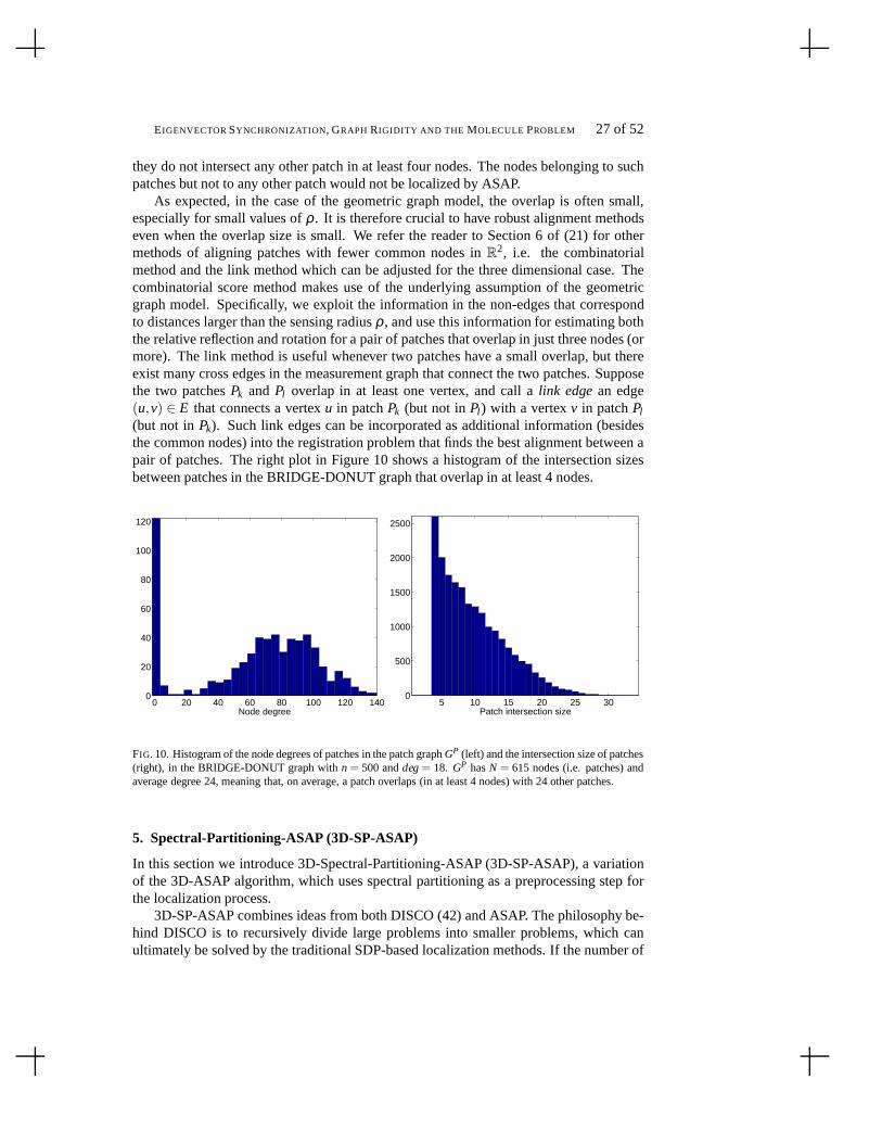
EIGENVECTORSYNCHRONIZATION, GRAPH RIGIDITY AND THE MOLECULE PROBLEM 27 of 52
they do not intersect any other patch in at least four nodes. The nodes belonging to suchpatches but not to any other patch would not be localized by ASAP.
As expected, in the case of the geometric graph model, the overlap is often small,especially for small values ofρ . It is therefore crucial to have robust alignment methodseven when the overlap size is small. We refer the reader to Section 6 of (21) for othermethods of aligning patches with fewer common nodes inR
2, i.e. the combinatorialmethod and the link method which can be adjusted for the threedimensional case. Thecombinatorial score method makes use of the underlying assumption of the geometricgraph model. Specifically, we exploit the information in thenon-edges that correspondto distances larger than the sensing radiusρ , and use this information for estimating boththe relative reflection and rotation for a pair of patches that overlap in just three nodes (ormore). The link method is useful whenever two patches have a small overlap, but thereexist many cross edges in the measurement graph that connectthe two patches. Supposethe two patchesPk and Pl overlap in at least one vertex, and call alink edgean edge(u,v) ∈ E that connects a vertexu in patchPk (but not inPl ) with a vertexv in patchPl
(but not inPk). Such link edges can be incorporated as additional information (besidesthe common nodes) into the registration problem that finds the best alignment between apair of patches. The right plot in Figure 10 shows a histogramof the intersection sizesbetween patches in the BRIDGE-DONUT graph that overlap in atleast 4 nodes.
0 20 40 60 80 100 120 1400
20
40
60
80
100
120
Node degree5 10 15 20 25 30
0
500
1000
1500
2000
2500
Patch intersection size
FIG. 10. Histogram of the node degrees of patches in the patch graphGP (left) and the intersection size of patches(right), in the BRIDGE-DONUT graph withn= 500 anddeg= 18. GP hasN = 615 nodes (i.e. patches) andaverage degree 24, meaning that, on average, a patch overlaps (in at least 4 nodes) with 24 other patches.
5. Spectral-Partitioning-ASAP (3D-SP-ASAP)
In this section we introduce 3D-Spectral-Partitioning-ASAP (3D-SP-ASAP), a variationof the 3D-ASAP algorithm, which uses spectral partitioningas a preprocessing step forthe localization process.
3D-SP-ASAP combines ideas from both DISCO (42) and ASAP. Thephilosophy be-hind DISCO is to recursively divide large problems into smaller problems, which canultimately be solved by the traditional SDP-based localization methods. If the number of

28 of 52 M. CUCURINGU, A. SINGER, AND D. COWBURN
atoms in the current group is not too large, DISCO solves the atom positions via SDP, andrefines the coordinates by using gradient descent; otherwise, it breaks the current groupof atoms into smaller subgroups, solves each subgroup recursively, aligns and combinesthem together, and finally it improves the coordinates by applying gradient descent. Themain question that arises is how to divide a given problem into smaller subproblems.DISCO chooses to divide a large group of nodes into exactly two subproblems, solveseach problem recursively and combines the two solutions. Inother words, it builds a bi-nary tree of problems, where the leaves are problems small enough to be embedded bySDP. However, not all available information is being used when considering only a singlespanning tree of the graph of patches. The 3D-ASAP approach fuses information fromdifferent spanning trees via the eigenvector computation.However, compared to the num-ber of patches used in DISCO, 3D-ASAP generates many more patches, since the numberof patches in 3D-ASAP is linear in the size of the network. This can be considered asa disadvantage, since localizing all the patches is often the most time consuming step ofthe algorithm. 3D-SP-ASAP tries to reduce the number of patches to be localized whileusing the patch graph connectivity in its full.
When dividing a graph into two smaller subgraphs, one wishesto minimize the num-ber of edges between the two subgraphs, since in the localization of the two subgraphs theedges across are being left out. Simultaneously, one wishesto maximize the number ofedges within the subgraphs, because this makes the subgraphs more likely to be globallyrigid and easier to localize. In general, the graph partitioning problem seeks to decomposea graph intoK disjoint subgraphs (clusters), while minimizing the number of cut edges,i.e., edges with endpoints in different clusters. We refer the reader to the literature on nor-malized cuts and spectral relaxations that can be computed efficiently (47; 57). We usethe spectral clustering method in (47) to partition the measurement graph in the moleculeproblem. The gist of the approach is to use the classical K-means clustering algorithm onthe Laplacian eigenmap embedding of the set of nodes. IfA is the adjacency matrix ofthe graphG, andD is a diagonal matrix withDi,i = deg(i), i = 1, . . . ,n, then the Laplacianeigenmap embedding of nodei in R
k is given by(φ1(i),φ2(i), . . . ,φK(i)), whereφ j is thejth eigenvector of the matrixD−1A. For an extensive literature survey on spectral clus-tering algorithms we refer the reader to (55). We remark thatother clustering algorithms(e.g., (33)) may also be used to partition the graph.
The approach we used for localization in conjunction with the above normalized spec-tral clustering algorithm is as follows (3D-SP-ASAP):
1. We first decompose the measurement graph intoK partitionsP1, . . . ,PK , usingthe normalized spectral clustering algorithm.
2. We extend each partitionPi , i = 1, . . . ,K to include its 1-hop neighborhood, anddenote the new patches byPi , i = 1, . . . ,K.
3. For every pair of patchesPi andPj which have nodes in common or are connected bylink edges13, we build a new (link) patch which contains all the common points andlink edges. The vertex set of the new patch consists of the nodes that are commonto bothPi andPj , together with the endpoints of the link edges that span across the
13edges with endpoints in different patches

EIGENVECTORSYNCHRONIZATION, GRAPH RIGIDITY AND THE MOLECULE PROBLEM 29 of 52
two patches. Note that the new list of patches contains the extended patches builtin Step (2)P1, . . . ,PK , as well as the newly built patchesPK+1, . . . ,PL.
4. We extract from each patchPi, i = 1, . . . ,L the WUL subgraph, and embed it usingthe FULL-SDP algorithm for noiseless data, and the SNL-SDP algorithm for noisydata.
5. Synchronize all available patches using the eigenvectorsynchronization algorithmused in ASAP.
Note that when the extended patches from Step (2) are highly overlapping, Step (3) ofthe algorithm should be omitted, for reasons detailed belowrelated to the robustness of theembedding. The reason for having Steps (2), and possibly (3), is to be able to align nearbypatches. Without Step (2) patches will have disjoint sets ofnodes, and the alignment willbe based only on the link edges, which is not robust for high levels of noise. Without Step(3) the existing patches may have little overlap, in which case we expect the alignmentinvolving link edges not to be robust at high levels of noise.By building the link patches,we provide 3D-SP-ASAP more accurate pairwise alignments. Note that embedding linkpatches is less robust to noise, due to their bipartite-likestructure, especially when thebipartitions are very loosely connected to each other (alsoconfirmed by our computationsinvolving link patches). In addition, having to localize a larger number of patches maysignificantly increase the running time of the algorithm. However, for our numericalexperiments with 3D-SP-ASAP conducted on the BRIDGE-DONUTgraph, the extendedpartitions built in Step (2) were highly overlapping, and allowed us to localize the entirenetwork without the need to build the link patches in Step (3).
The advantage of combining a spectral partitioning algorithm with 3D-ASAP is adecrease in running time as shown in Tables 13 and 14, due to a significantly smallernumber of patches that need to be localized. Note that the graph partitioning algorithm isextremely fast, and partitions the BRIDGE-DONUT measurement graph in less than halfa second. Table 11 shows the ANE reconstruction errors for the BRIDGE-DONUT graph,when we partition the measurement graph intoK = 8 andK = 25 clusters. ForK = 8,some of the extended partitions become very large, containing as many as 150 nodes,and SNL-SDP does a very poor job at embedding such large patches when the distancemeasurements are noisy. By increasing the number of partitions toK = 25, the extendedpartitions contain less nodes, and are small enough for SNL-SDP to localize accuratelyeven for high levels of noise. Note that the ANE errors for 3D-SP-ASAP withK = 25 arecomparable with those of ASAP, while the running time is dramatically reduced (by anorder of magnitude, for the BRIDGE-DONUT example withη = 35%). Figures 11 and12 show variousK-partitions of the PACM and the BRIDGE-DONUT graphs.
6. The Median Denoising Algorithm (MDA) and a Rescaling Heuristic
In this section we describe a method to improve the localization of the individual patchesprior to the patch alignment and global synchronization steps. The main observation hereis the following: suppose a pair of nodes appear in several different patches, then each

30 of 52 M. CUCURINGU, A. SINGER, AND D. COWBURN
(a) K=2 (b) K=3 (c) K=4 (d) K=5
(e) K=6 (f) K=7 (g) K=8 (h) K=9
FIG. 11. Partitions of the PACM graph (K is the number of partitions)
(a) K=2 (b) K=3 (c) K=4 (d) K=5
(e) K=6 (f) K=7 (g) K=8 (h) K=9
FIG. 12. Partitions of the BRIDGE-DONUT graph (K is the number of partitions)
patch provides a different estimation for their distance, and all these estimators can be av-eraged together to provide a perhaps more accurate estimator. The improved reestimateddistances are then used to localize the individual patches again, this time using the cMDSalgorithm since patches no longer contain any missing distances. The second part of thissection introduces a simple rescaling procedure, that increases the accuracy of the finalreconstruction.
Denote byCk (k= 1, . . . ,N) the set of all pairwise edges within patchPk (so if Pk hast nodes thenCk contains all
(t2
)edges). LetC denote the set of all edges that appear in
at least one patch, i.e.,C = ∪Nk=1Ck. Note thatC contains edges(i, j) that were initially
missing from the measurement set (i.e.(i, j) /∈ E) but for which we now have an estimatedue to the initial localization of the patches (using, say, SDP). After the initial embedding,we have at least one estimated distance for each edge(i, j) ∈ C , but because patchesoverlap, most of the edges appear in more than one patch. Denote byd1
i j ,d2i j , . . . the set

EIGENVECTORSYNCHRONIZATION, GRAPH RIGIDITY AND THE MOLECULE PROBLEM 31 of 52
of estimates for the (possibly missing) distance(i, j), wheredki j is the distance between
nodesi and j in the SDP embedding of patchPk. To obtain a more accurate estimate ofdi j we take the median of all the above estimates, and denote the updated value by
di j = median(d1i j ,d
2i j , . . .) (6.27)
If the noise level in the originally measured distances is small, then we expect theestimatesd1
i j ,d2i j , . . . to have small variance and take values close to the true distance.
However, for higher levels of noise, many of the estimates can be very inaccurate (eitherhighly overestimating or underestimating the true distances), and we choose the medianvalue to approximate the true distance. Tables 5 and 6 show that MDA is indeed effec-tive and reduces the noise level in the distances, usually byat least a few percentages.Note that the SDP improves by itself on the initial distance measurements (those that areavailable), and the MDA decreases their noise even further.
To take advantage of the more accurate updated distance values, we recompute theembeddings of allN patches using the cMDS algorithm, since there exists an estimate forall pairwise distances within a patch. Whenever a hard constrained distance (a “good”edge) is present, such as a bond length, we use its true distance in the cMDS embeddings,and ignore the noisy value returned by the SDP since hard constrained distances are notenforced in the SDP.
Tables 5 and 6 show the average ANE of the patches after the SDPembeddings(ANEold), and after the cMDS embeddings ran on the updated distances(ANEnew). Notethat the new patch embeddings are significantly more accurate, in some cases the ANEdecreasing by as much as 25%. We also experimented with an iterative version of thisdenoising algorithm, where at each round we run the cMDS and recompute the median ofthe updated distances. However, subsequent iterations of this procedure did not improvethe accuracy furthermore.
Existing distances Missing distancesη ANEold ANEnew η ηSDP ηMDA ηSDP ηMDA
10% 0.04 0.03 5.06 3.75 3.42 3.37 3.1320% 0.10 0.078 10.28 8.22 7.5 8.91 8.1230% 0.18 0.14 15.95 14.09 13.03 17.99 16.8340% 0.27 0.22 21.74 20.66 19.31 29.09 27.7250% 0.37 0.32 29.11 28.76 27.5 42.14 40.92
Table 5. Denoising distances at various levels of noise, forthe UNITCUBE data set.ANEold andANEnew
denote the average ANE of all patches after the SDP embeddingrespectively after the cMDS embedding withthe distances denoised by MDA.η is the empirical noise level (averaged over all noisy distances),ηSDP is thenoise level after the SDP embedding,ηMDA is the noise level after running MDA. We show the noise levelsindividually for both the existing and missing distances. Note thatη 6= η since the former denotes the averageabsolute value deviation from the true distance as a percentage of the true distance, while the latter is theparameter in the uniform distribution in (8.43) that is usedto define the noise model (in fact,E[η ] = η
2 ).
In the remaining part of this section, we discuss the issue ofscaling of the distances af-ter different steps of the algorithm, and propose a simple rescaling heuristic that improvesthe overall reconstruction.

32 of 52 M. CUCURINGU, A. SINGER, AND D. COWBURN
Existing distances Missing distancesη ANEold ANEnew η ηSDP ηSDP,GOOD ηMDA ηSDP ηMDA
0% 0.00048 0.00039 0 0.02 0.14 0 0.38 0.3210% 0.00316 0.00266 4.91 3.42 1.79 3.13 3.2 2.9920% 0.00590 0.00506 9.81 7.01 3.68 6.44 6.18 5.8130% 0.00957 0.00803 14.74 10.75 5.59 9.88 9.51 8.9540% 0.01292 0.01120 19.65 14.5 7.62 13.42 13.55 12.850% 0.01639 0.01462 24.57 18.1 9.82 16.93 18.24 17.35
Table 6. Denoising distances at various levels of noise for the ubiqutin (PDG 1d3z, (19)).ηSDP,GOOD denotesthe average noise of the hard constraint (“good”) distancesafter the SDP embeddings. Note that the currentimplementation of the SNL-SDP algorithm used for the patch embeddings does not allow for hard distanceconstraints.
We denote the true distance measurements byl i j = ‖pi − p j‖,(i, j) ∈ E, and the em-pirical measurements bydi j = l i j + εi j ,(i, j) ∈ E, whereεi j is random independent noise,as introduced in (8.43). We generically refer todi j as the distance between nodesi and j,after different steps of the algorithm, as indicated by the columns of Tables 7 and 8. Wedenote byδ the average scaling of the distances with respect to their ground truth values,and similarly byκ the average empirical noise of the distance measurements
δ = mean
(l i jdi j
,(i, j) ∈ E
), κ = mean
(∣∣∣∣di j − l i j
l i j
∣∣∣∣ ,(i, j) ∈ E
)
The first column of the tables contains the scaling and noise values of the initial dis-tance measurements, taken as input by ASAP. The fact thatκ is approximately half thevalue of the noise levelη stems from the fact that the measurements are uniformly dis-tributed in[(1−η)l i j ,(1+η)l i j ]. Note that the initial scaling is quite significant, and thisis a consequence of the same noise model and the geometric graph assumption. Distancesthat are scaled down by the noise will still be available to 3D-ASAP, while distances thatare scaled up and become larger than the sensing radius will be ignored. Therefore, onaverage, the empirical distances are scaled down andδ is greater than 1.
The second column gives the scaling and noise values after the MDA algorithm fol-lowed by cMDS to recompute the patches. Note that after this denoising heuristic, whilethe scalingδ remains very similar to the original values, the noiseκ decreases consider-ably especially for the lower levels of noise.
The third column computes the scaling, noise and ANE values after the least squaresstep for estimating the translations, where by ANE we mean the average normalized errorintroduced in (8.44). Note that both the scaling and the noise levels significantly increaseafter integrating all patches in a globally consistent framework. To correct the scalingissue, we scale up all the available distances (thus taking into account only the edges ofthe initial measurement graph) byδ ∗, computed as
δ ∗ = mean
(di j
dLSi j
,(i, j) ∈ E
)
wheredi j denotes the initial distances, anddLSi j the distances after the least-square step.

EIGENVECTORSYNCHRONIZATION, GRAPH RIGIDITY AND THE MOLECULE PROBLEM 33 of 52
Note that, as a consequence, the ANE error of the reconstruction decreases significantly.Finally, we refine the solution by running gradient descent,on the initial distancesdi j
scaled up byδ ∗, which further improves the scaling, noise and ANE values.
Original MDA-cMDS Least squares Rescaled Gradient Descentη% δ κ% δ κ% δ κ% ANE δ ∗ ANE δ κ% ANE
10 1.01 5.1 1.01 3.4 1.02 3.6 0.05 1.01 0.05 1.00 3.0 0.0420 1.05 10.3 1.04 7.5 1.08 8.8 0.12 1.04 0.10 1.02 6.1 0.0730 1.12 16.0 1.11 13.0 1.21 17.0 0.25 1.09 0.20 1.04 9.9 0.1640 1.22 21.8 1.21 19.3 1.43 27.8 0.36 1.21 0.26 1.04 13.9 0.1945 1.29 26.0 1.28 23.8 1.65 35.6 0.45 1.32 0.30 1.02 17.8 0.2650 1.38 29.2 1.36 27.5 1.92 43.8 0.53 1.47 0.35 0.99 22.4 0.32
Table 7. Average scaling and noise of the existing edges (andwhere appropriate the ANE of the reconstruction)for the UNITCUBE graph, at various steps of the algorithm: after the original measurements, after the SDP-MDA-cMDS denoising step, after the least squares in Step 3, after rescaling of the available distances by theempirical scaling factorδ ∗, and after running gradient descent on the rescaled (originally available) distances.
Original MDA-cMDS Least squares Rescaled Gradient Descentη% δ κ% δ κ% δ κ% ANE δ ∗ ANE δ κ% ANE
10 1.00 0.03 1.00 0.02 1.02 0.04 0.01 1.02 4e-3 0.99 0.01 3e-320 1.01 0.06 1.00 0.04 1.04 0.07 0.01 1.03 0.01 0.99 0.02 0.0130 1.02 0.08 1.01 0.06 1.06 0.10 0.02 1.05 0.01 0.99 0.03 0.0140 1.03 0.11 1.01 0.08 1.10 0.14 0.02 1.09 0.02 0.99 0.05 0.0150 1.06 0.14 1.02 0.10 1.18 0.19 0.04 1.16 0.03 0.98 0.08 0.01
Table 8. Average scaling and noise of all edges (good+NOE) ofthe ubiqutin (PDG 1d3z) (and where appropri-ate the ANE of the reconstruction) at various steps of the algorithm: after the original measurements, after theSDP-MDA-cMDS denoising step, after the least squares in Step 3, after rescaling of the available distances bythe empirical scaling factorδ ∗, and after running gradient descent on the rescaled NOE distances.
7. Synchronization with molecular fragments
In the molecule problem, as mentioned earlier, there are molecular fragments whose localconfiguration is known in advance up to an element of the special Euclidean group SE(3)rather than the Euclidean group E(3). In other words, these are small structures that needto be translated and rotated with respect to the global coordinate system, but no reflec-tion is required. As a result, for their corresponding patches we know the correspondinggroup element inZ2. This motivates us to consider the problem of synchronization overZ2 when “molecular fragment” information is available, and refer to it from now on asSYNC(Z2). We propose and compare four methods for solving SYNC(Z2): two relax-ations to a quadratically constrained quadratic program (QCQP), and two semidefiniteprogramming (SDP) formulations.
Mathematically, the synchronization problem over the groupZ2 = {±1} can be statedas follows: givenk group elements (anchors)A = {a1, . . . ,ak} and a set of (possibly) in-

34 of 52 M. CUCURINGU, A. SINGER, AND D. COWBURN
complete (noisy) pairwise group measurementszi j = aix−1j andzi j = xix−1
j , (i, j) ∈ E(G),find the unknown group elements (atoms)S = {x1, . . . ,xl}. We may sometimes abusenotation and denote all nodes byx= {x1, . . . ,xl ,xl+1, . . . ,xN}, whereN = l + k, with theunderstanding that the lastk elements denote the anchors. Whenever we say that indicesi ∈ S and j ∈ A , it should be understood that we refer to atomsxi ∈ S , respectivelyanchora j ∈ A . In the molecule problem,k denotes the number of patches whose reflec-tion is known a priori, and the goal is to estimate the reflection of the remainingl = N−kpatches.
7.1. Synchronization by relaxing a QCQP
When anchor information is available, meaning that we know apriori some of the groupelements which we refer to as anchors, we follow a similar approach to the objective func-tion that motivated the eigenvector synchronization method. Similarly, we are interestedin finding the set of unknown elements that maximize the number of satisfied pairwisemeasurements, but this time, under the additional constraints imposed by the anchors,i.e. xi = ai , i ∈ A . Unfortunately, maximizing the quadratic formxTZx under the anchorconstraints, is no longer an eigenvector problem. Our approach is to combine under thesame objective function both the contribution of the atom-atom pairwise measurements(as a quadratic term) and the contribution of the anchors-atom pairwise measurements (asa linear term). To that end, we start by formulating the synchronization problem as a leastsquares problem, by minimizing the following quadratic form
minx ∑
(i, j)∈E
(xi −Zi j x j)2 = min
x ∑(i, j)∈E
z2i +Z2
i j x2j −2Zi j xix j
= minx ∑
(i, j)∈E
x2i + x2
j −2Zi j xix j
= minx
n
∑i=1
dix2i − ∑
(i, j)∈E
2Zi j xix j
= minx
xTDx− xTZx
= minx
xT(D−Z)x (7.28)
To account for the existence of anchors, we first write the matricesZ andD in the follow-ing block format
Z =
[S U
UT V
], D =
[DS 00 DV
]
whereSl×l ,Ul×k andVk×k denote the atom-atom, atom-anchor respectively anchor-anchormeasurements, andD is a diagonal matrix withDii = ∑N
j=1 |Zi j |. Note thatV is a matrixwith all nonzero entries, since the measurement between anytwo anchors is readily avail-able. Similarly, we write (with a slight abuse of notation) the solution vector in the formx = [s a]T , wheres denotes the signs of the atom nodes, anda the signs of the anchornodes. The quadratic function minimized in (7.28) can now bewritten in the following

EIGENVECTORSYNCHRONIZATION, GRAPH RIGIDITY AND THE MOLECULE PROBLEM 35 of 52
form
[sT aT
][ DS−S −U−UT DV −V
][sa
]= sT(DS−S)s−2sTUa+aT(DV −V)a (7.29)
The vector(Ua)l×1 can be interpreted as the anchor contribution in the estimation of theatoms. Note that in the case when the atom-anchor measurements should be trusted morethan the atom-atom measurements, the anchor contribution can be weighted accordingly,and equation (7.29) becomeszT(DS−S)z−2γzTUa+aT(DV −V)a, for a given weightγ. SinceaT(DV −V)a is a (nonnegative) constant, we are interested in minimizing theinteger quadratic form
minimizez∈Zl
2
zT(DS−S)z−2zTUa.
Unfortunately, solving such a problem is NP-hard, and thus we introduce the followingrelaxation to a quadratically constrained quadratic program (QCQP)
minimizez=(z1,...,zl )
zT(DS−S)z−2zTUa
subject to zTz= l(7.30)
We proceed by considering the Lagrangian function
φ(z,λ ) = zT(DS−S)z−2zTUa+λ (zTz− l) (7.31)
whereλ is the Lagrange multiplier. Differentiating (7.31) with respect toz, we are led tothe following equation
2(DS−S)z−2Ua+2λz= 0
which can be written as(DS−S+λ I)z=Ua (7.32)
Using the fact thatzTz= l , (7.32) becomes
(Ua)T(DS−S+λ I)−2(Ua) = l (7.33)
which we solve forλ . We refer the reader to (6) for a more detailed analysis of eigenvaluesolutions to such quadratically constrained optimizationproblems. Finally, the solutionto the minimization problem formulated in (7.30) is given by
z∗ = (DS−S+λ I)−1(Ua) (7.34)
For simplicity, we choose to solve the nonlinear matrix equality (7.33) in MATLAB usingthe lsqnonlincommand, whose success in findingλ is contingent upon a good initializa-tion. To that end, we consider the eigendecomposition of thesymmetric positive definitematrix
DS−S=l
∑i=1
λiφiφTi ,
36 of 52 M. CUCURINGU, A. SINGER, AND D. COWBURN
where(D−S)φi = λiφi , for i = 1, . . . , l , and expand the vectorsUa andz in the formUa = ∑l
i=1 βiφi andz= ∑li=1 αiφi . Rewriting equation (7.32),(DS−S)z+λz= Ua, in
terms of the above expansion yields
l
∑i=1
λiαiφi +λl
∑i=1
αiφi =l
∑i=1
βiφi . (7.35)
Thus, for everyi = 1, . . . , l it must hold true that
λiαi +λ αi = βi , (7.36)
i.e. αi =βi
λ+λi. SincezTz= l and∑l
i=1 α2i = l , the Lagrange multiplierλ must satisfy
l
∑i=1
β 2i
(λ +λi)2 = l (7.37)
The condition thatλ +λi > 0 ensures that the solution search forλ lies outside the set ofsingularities of (7.37). Thusλ > −λ0, whereλ0 is the smallest eigenvalue of the matrixDS−S. Note that the row sums ofDS−Sare non-negative since the diagonal entries inDS are the degree of the atom nodes in the entire graph, taking into account the atom-anchor edges as well, not just the atom-atom edges. Furthermore,DS−S is a positivesemidefinite matrix (thusλ0 > 0), as it can be seen from the following identity
xT(DS−S)x =l
∑i=1
x2i di − ∑
(i, j)∈ESS
2xix jSi j > ∑(i, j)∈ESS,Si j=±1
(xi −Si j x j)2> 0
whereESSdenotes the set of atom-atom edges.We also consider the following formulation similar to (7.30), but we replace the con-
straintzTz= l with zTDSz= ∆ , where∆ = ∑li=1di is the sum of the degrees of all atom
nodes. Note that the following change of variable ¯z= D1/2S z brings the new optimization
problem to a form similar to (7.30)
minimizez
zTD−1/2S (DS−S)D−1/2
S z−2zTD−1/2S Ua
subject to ¯zT z= ∆(7.38)
with the corresponding Lagrangianλ satisfyingλ >−λ0, whereλ0 is the smallest eigen-
value of the matrixD−1/2S (DS−S)D−1/2
S .
7.2. Synchronization by SDP
An alternative approach to solving SYNC(Z2) is by using semidefinite programming.The connection between the Lagrangian relaxation of the QCCP shown in the previoussection, and the SDP relaxation we are about the introduce was investigated in (23) andthe references therein. The minimization of the least squares objective function in (7.28)is equivalent to the maximization of the following objective function
N
∑i, j=1
xiZi j x j = Trace(Zϒ ) (7.39)

EIGENVECTORSYNCHRONIZATION, GRAPH RIGIDITY AND THE MOLECULE PROBLEM 37 of 52
whereϒ is theN×N symmetric rank-one matrix with±1 entries
ϒi j =
xix−1j if i, j ∈ S
xia−1j if i ∈ S , j ∈ A
aia−1j if i, j ∈ A
(7.40)
Note thatϒ has ones on its diagonalϒii = 1,∀i = 1, . . . ,N, and the anchor informationgives another layer of hard constraints. The SDP relaxationin the presence of anchorsbecomes
maximizeϒ∈RN×N
Trace(Zϒ )
subject to ϒii = 1, i = 1, . . . ,N
ϒi j = aia−1j , if i, j ∈ A
ϒ � 0
(7.41)
where the maximization is taken over all semidefinite positive real-valued matricesϒ � 0.While ϒ as defined in (7.41) has rank one, the solution of the SDP is notnecessarily ofrank one. We therefore compute the top eigenvector of that matrix, and estimatex1, . . . ,xs
based on the sign of its firstsentries.Alternatively, to reduce the number of unknowns in (7.41) from N = l + k to l , one
may consider the following relaxation
maximizeϒ∈Rl×l ;x∈Rl
Trace(Sϒ)+2xTUa
subject to ϒii = 1,∀i = 1, . . . , l[
ϒ xxT 1
]� 0
(7.42)
Ideally, we would like to enforce the constraintϒ = xxT , which guarantees thatϒ is indeeda rank-one solution. However, since rank constrains do not lead to convex optimizationproblems, we relax this constraint via Schur’s lemma toϒ � zzT . This last matrix inequal-ity is equivalent (16) to the last constraint in the SDP formulation in (7.42). Finally, weobtain estimators ˆz1, . . . , zl for the atoms by setting ˆzi = sign(xi),∀i = 1, . . . , l .
7.3. Comparison of algorithms for SYNC(Z2)
Figure 13 compares the performance of the algorithms we proposed for synchronizationin the presence of molecular fragment information. The adjacency graph of availablepairwise measurements is an Erdos-Renyi graphG(N, p) with N = 75 andp= 0.2 (i.e.,a graph withN nodes, where each edge is present with probabilityp, independent ofthe other edges). We show numerical experiments for four scenarios, where we vary thenumber of anchorsk = {5,15,30,50} chosen uniformly at random from theN nodes.As the number of anchors increases, compared to the number ofatomss= N− k, theperformance of the four algorithms is essentially similar.Only when the number of an-chor nodes is small (k= 5), the SDP-Y formulation shows superior results, togetherwithSDP-XY and QCQP with constraintzTDz= ∆ , while the QCQP with constraintzTz= sperforms less well. In practice, one would choose the QCQP formulation with constraint

38 of 52 M. CUCURINGU, A. SINGER, AND D. COWBURN
zTDz= ∆ , since the SDP based methods are computationally expensiveas the size ofthe problem increases. This was also our method of choice forcomputing the reflectionof the patches in the localization of the ubiqutin (PDG 1d3z), when molecular fragmentinformation was available and the reflection of many of the patches was known a priori .
10 20 30 40
0.1
0.2
0.3
0.4
Noise level η
Err
or r
ate
τ
k = 5
SDP−YSDP−XYQCQP zTzQCQP zT D z
10 20 30 400
0.1
0.2
0.3
0.4
Noise level η
Err
or r
ate
τ
k = 15
SDP−YSDP−XYQCQP zTzQCQP zT D z
10 20 30 400
0.1
0.2
0.3
0.4
Noise level η
Err
or r
ate
τ
k = 30
SDP−YSDP−XYQCQP zTzQCQP zT D z
10 20 30 400
0.1
0.2
0.3
0.4
Noise level η
Err
or r
ate
τ
k = 50
SDP−YSDP−XYQCQP zTzQCQP zT D z
FIG. 13. Comparison, in terms of robustness to noise, of the fouralgorithms we proposed for SYNC(Z2): thetwo QCQP formulations using the two different constraints:zTz= s andzTDz= ∆ as they appear in equations(7.30) and (7.38), the two SDP-based formulations SDP-Y andSDP-XY as formulated in (7.41) and (7.42). Theadjacency graph of available pairwise measurements is an Erdos-Renyi graphG(N, p) with N = 75 andp= 0.2.Also, k denotes the number of anchors, chosen uniformly at random from theN nodes. Results are averagedover 50 runs.
8. Experimental results
We have implemented our 3D-ASAP algorithm and compared its performance with othermethods across a variety of measurement graphs, varying parameters such as the numberof nodes, average degree (sensing radius) and level of noise.
In our experiments, the noise is multiplicative and uniform, meaning that to each truedistance measurementl i j =‖ pi − p j ‖, we add random independent noiseεi j in the range

EIGENVECTORSYNCHRONIZATION, GRAPH RIGIDITY AND THE MOLECULE PROBLEM 39 of 52
[−η l i j ,η l i j ], i.e.,
di j = l i j + εi j
εi j ∼Uni f orm([−η l i j ,η l i j ]) (8.43)
The percentage noise added is 100η , (e.g.,η = 0.1 corresponds to 10% noise).The sizes of the graphs we experimented with range from 200 to1000 nodes taking
different shapes, with average degrees in the range 14−26, and noise levels up to 50%.Across all our simulations, we consider the geometric graphmodel, meaning that all pairsof nodes within rangeρ are connected. Note that all the graphs considered throughout thepaper are three-dimensional, even if they visually look two-dimensional in the attachedfigures.
We denote the true coordinates of all nodes by the 2×n matrix P= (p1 · · · pn), andthe estimated coordinates by the matrixP = (p1 · · · pn). To measure the localizationerror of our algorithm we first factor out the optimal rigid transformation between thetrue embeddingP and our reconstructionP, and then compute the following averagenormalized error (ANE)
ANE=
√∑n
i=1 ‖ pi − pi ‖2√
∑ni=1 ‖ pi − p0 ‖2
=‖ P− P ‖F
‖ P− p01T ‖F, (8.44)
wherep0 = 1n ∑n
i=1 pi is the center of mass of the true coordinates. The normalizationfactor in the denominator of (8.44) ensures that the ANE is not only rigid invariant, but itis also scale free, i.e., it is invariant to scaling the underlying configuration by a constantfactor.
The experimental results in the case of noiseless data (i.e.incomplete set of exactdistances) should already give the reader an appreciation of the difficulty of the problem.As mentioned before, the graph realization problem is NP-hard, and the most we can aimfor is an approximate solution. The main advantage of introducing the notion of a weaklyuniquely localizable graph and using it for breaking the original problem into smallersubproblems, can be seen in the experimental results for noiseless data. Note that acrossall experiments, except for the PACM graph reconstructions, we are able to computelocalizations which are at least one order of magnitude moreaccurate than what thosecomputed by DISCO or SNL-SDP. Note that all algorithms are followed by a refinementprocedure, in particular steepest descent with backtracking line search.
As expected, FAST-MVU performs at its best when the data is a set of random pointsuniformly distributed in the unit cube. In this case, the topthree eigenvectors of theLaplacian matrix used by FAST-MVU provide an excellent approximation of the originalcoordinates. Indeed, as the experimental results in Table 9show, the FAST-MVU algo-rithm gives the best precision across all algorithms, returning anANE= 2e−6. However,in the case of noisy data, the performance of FAST-MVU degrades significantly, makingFAST-MVU the least robust to noise algorithm tested on the UNITCUBE graph. Fur-thermore, FAST-MVU performs extremely poor on more complicated topologies, even inthe absence of noise, as it can be seen in the reconstructionsof the PACM and BRIDGE-DONUT graphs shown in Figure 14. For comparison, the original underlying graphs areshown in Figures 15 and 16.
40 of 52 M. CUCURINGU, A. SINGER, AND D. COWBURN
η 3D-ASAP DISCO SNL-SDP MVU
0% 5e-4 8e-3 2e-3 2e-610% 0.04 0.06 0.04 0.0720% 0.07 0.10 0.09 0.1230% 0.16 0.17 0.17 0.2640% 0.19 0.29 0.29 0.5045% 0.26 0.34 0.35 0.4850% 0.32 0.42 0.43 0.61
Table 9. Reconstruction errors (measured inANE) for theUNITCUBE graphs withn= 212 vertices, sensing radiusρ = 0.3 and average degreesdeg= 17−25.
η 3D-ASAP DISCO
0 % 0.0001 0.002410 % 0.0031 0.002920 % 0.0052 0.005830 % 0.0069 0.007835 % 0.0130 0.010440 % 0.0094 0.010745 % 0.0168 0.020750 % 0.0146 0.0151
Table 10. Reconstruction errors (measuredin ANE) for the 1d3z molecule graph withn = 1009 vertices, sensing radiusρ = 5angstrom and average degreedeg= 14.
−6 −4 −2 0 2 4 6 8
−2
0
2
(a) PACM graph with noiseη = 0%
−2 0 2 4
−3
−2
−1
0
1
2
3
4
(b) DONUT graph with noiseη = 0%
FIG. 14. Reconstructions of the PACM and BRIDGE-DONUT graphs using the FAST-MVU algorithm, in thecase of noiseless data (compare to the original measurementgraphs shown in Figures 15 and 16.)
The second data set used in our experiments is a synthetic example of the moleculeproblem, and represents the ubiqutin protein represented by PDB entry 1d3z (19), with1288 atoms, 686 of which are hydrogen atoms. However, after removing the nodes of de-gree less than 4,n= 1009 atoms remain. For this data set, the available distances can bedivided into groups: the first group contains distances inferred from known bond lengthand torsion angles (“good” edges) which are kept accurate across different levels of noise,and the second group contains distances (NOE edges) which are perturbed with noiseηat each stage of the experiment. On average, each node is incident with 6 good edgesand 8 NOE edges, thus the average degree of the entire measurement graph isdeg= 14.In addition, besides knowledge of good and NOE edges, we alsouse information frommolecular fragments in the form of subgroups of atoms (molecular fragments) whosecoordinates are readily available. We incorporate 280 suchmolecular fragments, whoseaverage size is close to 5 atoms. To exploit such information, we slightly modify the ap-proach to break up the measurement graph and synchronize thepatches. We build patchesfrom molecular fragments by selecting a WUL subgraph from each extended molecularfragment, where by an extended molecular fragment we mean the graph resulting froma molecular fragment and all its 1-hop neighbors. Once we extract patches from all ex-

EIGENVECTORSYNCHRONIZATION, GRAPH RIGIDITY AND THE MOLECULE PROBLEM 41 of 52
tended molecular fragments, we consider all remaining nodes (singletons) that are notcontained in any of the patches obtained so far. Depending onthe noise level, the numberof such singleton nodes is between 10 and 15. Finally, we extract WUL patches fromthe 1-hop neighborhoods of the singleton nodes, following the approach of Section 4..Since we know a priori the localization, and in particular the reflection of each molecularfragment, and the reflection of a molecular fragment inducesa reflection on the patch thatcontains it, we have readily available information on the reflection of all patches that con-tain molecular fragments. In other words, we are solving a synchronization problem overZ2 when molecular fragment information is available. Using the synchronization methodintroduced in Section 7.1., we compute the reflection of the remaining patches. In termsof the reconstruction error, 3D-ASAP and DISCO return comparable results, slightly infavor of our algorithm. For noiseless NOE distances, we compute a localization that isone order of magnitude more accurate than the solution returned by DISCO.
Another graph that we tested is the BRIDGE-DONUT graph shownin Figure 16. Ithasn = 500 nodes, sensing radiusρ = 0.92, and average degree in the range 18− 25,depending on the noise level. Table 11 contains the reconstruction errors for variouslevels of noise showing that 3D-ASAP consistently returns more accurate solutions thanDISCO. For the BRIDGE-DONUT graph, we included in our numerical simulations thespectral partitioning 3D-SP-ASAP algorithm, which performed just as well as the 3D-ASAP algorithm (while significantly reducing the running time as shown in Tables 14and 13), and consistently outperformed the DISCO algorihtmat all levels of noise. Notethat 3D-SP-ASAP returns very poor localizations when usingonly k = 8 partitions; inthis case the extended partitions have large size (up to 150 nodes) and SNL-SDP fails toembed them accurately, even at small levels of noise, as shown in Table 11. By increasingthe number of partitions fromk= 8 tok= 25 and thus decreasing the size of each partition(and also of the extended partitions), the running time of 3D-SP-ASAP increases slightlyfrom 140 to 186 seconds (at 35% noise), but we are now able to match the accuracy of3D-ASAP which requires almost ten times more running time (1770 seconds).
Finally, for the PACM graphs in Figure 15, the network takes the shape of the lettersP,A,C,M that form a connected graph onn= 800 vertices. The sensing radius isρ = 1.2and the average degree in the rangedeg≈ 21−26. This graph was particularly useful intesting the sensitivity of the algorithm to the topology of the network. In Table 12, weshow the reconstruction errors for various levels of noise DISCO returns better results forη = 0%,10%,40%, but less accurate forη = 20%,30%,35%. We believe that DISCOreturns results comparable to 3D-ASAP (unlike the previousthree graphs) because thetopology of the PACM graph favors the graph decomposition used by DISCO. Note thatatη = 0% noise, the 3D-ASAP reconstruction differs from the original embedding mainlyin the right handside of the letter M, which is loosely connected to the rest of the letter,and also parts of its underlying graph are very sparse, thus rendering the SDP localizationalgorithms less accurate. This can also be seen in the spectral partitioning of the PACMgraph shown in Figure 11, where fork (number of clusters) as low as 3 or 4, the right sideof letter M is picked up as an individual cluster. At higher levels of noise 3D-SP-ASAPproves to be more accurate than DISCO, and it returns resultscomparable with ASAP.
Table 14 shows the running time of the various steps of the 3D-ASAP algorithm corre-
42 of 52 M. CUCURINGU, A. SINGER, AND D. COWBURN
η 3D-ASAP 3D-SP-ASAPk=8 3D-SP-ASAPk=25 DISCO
0% 6e-4 4e-4 2e-4 4e-310% 0.04 0.59 0.03 0.0320% 0.05 0.48 0.04 0.0730% 0.11 0.52 0.14 0.3035% 0.12 0.33 0.15 0.2140% 0.24 0.42 0.19 0.2745% 0.28 0.71 0.32 0.3550% 0.23 0.35 0.35 0.40
Table 11. Reconstruction errors (measured inANE) for the BRIDGE-DONUT graph withn = 500vertices, sensing radiusρ = 0.92 and average degreesdeg= 18−25. We usedk to denote the numberof partitions of the vertex set. Forη = 0 we embed each of thek patches (extended partitions) usingFULL-SDP, while for η > 0 we used the SNL-SDP algorithm. Atη = 50%, 3D-SP-ASAPk=8localizes only 435 out of the 500 nodes.
η 3D-ASAP 3D-SP-ASAPk=40 DISCO
0% 0.05 0.05 0.0210% 0.08 0.12 0.0720% 0.07 0.16 0.1830% 0.27 0.15 0.4535% 0.18 0.32 0.2840% 0.48 0.20 0.26
Table 12. Reconstruction errors (measured inANE) for the PACM graph withn = 800 vertices,sensing radiusρ = 1.2 and average degreesdeg= 21− 26. For 3D-SP-ASAP we usedk = 40partitions. Note that even for the noiseless case the error is not negligible due to incorrect embeddingsof subgraphs that are contained in the right leg of the letterM.
sponding to our not particularly optimized MATLAB implementation. Our experimentalplatform was a PC machine equipped with an Intel(R) Core(TM)2 Duo CPU E8500 @3.16GHz 4 GB RAM. Notice that all steps are amenable to a distributed implementation,thus a parallelized implementation would significantly reduce the running times. Note therunning time of 3D-ASAP is significantly larger than that of 3D-SP-ASAP and DISCO,due to the large number of patches (linear in the size of the network) that need to be lo-calized. 3D-SP-ASAP addresses this issue, and reduces the running time from 474 to 108seconds (forη = 0%), and from 1770 to 186 seconds (forη = 35%). Note that all stepsof the algorithm scale linearly in the size of the network, except for the eigenvector com-putation, which is nearly-linear. We refer the reader to Section 7 of (21) for a complexityanalysis of each step of 2D-ASAP, and remark that it is very similar to the complexity of3D-ASAP.
9. Summary and discussion
In this paper, we introduced 3D-ASAP (As-Synchronized-As-Possible), a novel divideand conquer, non-incremental non-iterative anchor-free algorithm for solving (ab-initio)the molecule problem. In addition, we also proposed 3D-SP-ASAP, a faster version of3D-ASAP, which uses a spectral partitioning algorithm as a preprocessing step for divid-ing the initial graph into smaller subgraphs. Our extensivenumerical simulations show

EIGENVECTORSYNCHRONIZATION, GRAPH RIGIDITY AND THE MOLECULE PROBLEM 43 of 52
Number of partitionsk k= 8 k= 25Noise levelη 0% 35% 35%Spectral partitioning 0.3 0.3 0.7Finding WUL subgraphs 48 81 89Embedding FULL-SDP 53 (82) (89)Embedding SNL-SDP (26) 50 86Step 1 (Z2×S0(3) ) 1 1 1Step 2 (Least squares) 6 8 9Total 108 140 186
Table 13. Running times (in seconds) of the 3D-SP-ASAP algorithm for the BRIDGE-DONUT graph withn= 500 nodes,η = 0%,35%,deg= 18,21, andk= 8,25 partitions. Forη = 0% we embed the patches usingFULL-SDP, while forη = 35% we use SNL-SDP since the regularization term improves the localization.
η = 0% η = 35%BreakG into patches 59 90Finding WUL subgraphs 210 233Embedding FULL-SDP 154 (252)Embedding SNL-SDP (966) 1368Denoising patches 30 39Step 1 (Z2×S0(3) ) 15 19Step 2 (Least squares) 6 213D-ASAP 474 1770
DISCO 196 1973D-SP-ASAP 108 186
Table 14. Running times (in seconds) of the 3D-ASAP algorithm for the BRIDGE-DONUT graph withn = 500 nodes,η = 0%,35%, deg= 18,21, N = 533,541 patches, and average patch sizes 17.8,20.3. Forη = 0% we embed the patches using FULL-SDP, while forη = 35% we use SNL-SDP since the regularizationterm improves the localization. Forη = 35%, during the least squares step we also use the scaling heuristic,and run the gradient descent algorithm several times, hencethe increase in the running time from 6 to 21seconds.
that 3D-ASAP and 3D-SP-ASAP are very robust to high levels ofnoise in the measureddistances and to sparse connectivity of the measurement graph.
We build on the approach used in 2D-ASAP to accommodate for the additional chal-lenges posed by rigidity theory inR3 as opposed toR2. In particular, we extract patchesthat are not only globally rigid, but also weakly uniquely localizable, a notion that is basedon the recent unique localizability of So and Ye (52). In addition, we also increase therobustness to noise of the algorithm by using a median-baseddenoising algorithm in thepreprocessing step, by combining into one step the methods for computing the reflectionsand rotations, thus doing synchronization over O(3)=Z2× SO(3) rather than individuallyoverZ2 followed by SO(3), and finally by incorporating a scaling correction in the finalstep where we compute the translations of each patch by solving an overdetermined linearsystem by least squares. Another feature of 3D-ASAP is beingable to incorporate readilyavailable structural information on various parts of the network.
Furthermore, in terms of robustness to noise, 3D-ASAP compares favorably to someof the current state-of-the-art graph localization algorithms. The 3D-ASAP algorithm

44 of 52 M. CUCURINGU, A. SINGER, AND D. COWBURN
follows the same “divide and conquer” philosophy that is behind our previous 2D-ASAPalgorithm, and starts with local coordinate computations based only on the 1-hop neigh-borhood information (of a single node, or set of nodes whose coordinates are known a pri-ori ), but unlike previous incremental methods, it synchronizes all such local informationin a noise robust global optimization process using an efficient eigenvector computation.In the preprocessing step of doing the local computations, amedian-based denoising al-gorithm improves the accuracy of the patch reconstructions, previously computed by theSDP localization algorithm.
Across almost all graphs that we have tested, 3D-ASAP constantly gives better resultsin terms of the averaged normalized error of the reconstruction. Except for the PACMgraph, whose topology greatly favors the divide and conquerapproach used by DISCO,3D-ASAP returns reconstructions that are often significantly more accurate in the pres-ence of large noise. Furthermore, for the case of noiseless distance measurements, thenotion of weakly uniquely localizable graphs that we introduced, leads to reconstructionsthat are an order of magnitude more accurate than DISCO and SNL-SDP.
The geometric graph assumption, which comes up naturally inmany problems ofpractical interest, is essential to the performance of the 3D-ASAP algorithm as it favorsthe existence of globally rigid or WUL patches of relativelylarge size. When the geomet-ric graph assumption does not hold, the 1-hop neighborhood of a node may be extremelysparse, and thus breaking up such a sparse star graph leads tomany small patches (i.e.,most of them may contain only a few nodes), with only a few of them having a largeenough pairwise intersection. Since small patches lead to small patch intersections, itwould therefore be difficult for 3D-ASAP to align patches correctly and compute a ro-bust final solution. Note that in the case of random Erdos-R´enyi graphs we expect theSDP methods, or even the low-rank matrix completion approaches, to work well. In otherwords, while these methods rely on randomness, our 3D-ASAP algorithm benefits fromstructure the most.
For the molecule problem, while 3D-ASAP can benefit from any existing molecularfragments, there is still information that it does not take advantage of, and which can fur-ther improve the performance of the algorithm. The most important information missingfrom our 3D-ASAP formulation are the residual dipolar couplings (RDC) measurementsthat give angle information (cos2(θ )) with respect to a global orientation. Another pos-sible approach is to consider an energy based formulation that captures the interactionbetween pairs of atoms (e.g. Lennard-Jones potential), anduse this information to betterlocalize the patches.
Another information one may use to further increase the robustness to noise is thedistinction between the “good” and “noisy” edges. There aretwo parts of the algorithmthat can benefit from such information. First, in the preprocessing step for localizing thepatches one may enforce the “good” distances as hard constraints in the SDP formulation.Second, in the step that synchronizes the translations using least squares, one may chooseto give more weight to equations involving the “good” edges,keeping in mind howeverthat such equations are not noise free since the direction ofan edge may be noisy as aresult of steps 1 and 2, even if the distances are accurate. However, note that 3D-ASAPdoes use the “good” edges as hard constraints in the gradientdescent refinement at theend of step 3.
One other possible future direction is combining the reflection, rotation and translation

EIGENVECTORSYNCHRONIZATION, GRAPH RIGIDITY AND THE MOLECULE PROBLEM 45 of 52
steps into a single step, thus doing synchronization over the Euclidean group. Our currentapproach in 3D-ASAP takes one step in this direction, and combines the reflection androtations steps by doing synchronization over the Orthogonal group O(3). However, incor-porating the translations step imposes additional challenges due to the non-compactnessof the group Euc(3), rendering the eigenvector method no longer applicable directly.
In general, there exist very few theoretical guarantees forgraph localization algo-rithms, especially in the presence of noise. A natural extension of this paper is a theoret-ical analysis of ASAP, including performance guarantees interms of robustness to noisefor a variety of graph models and noise models. However, a complete analysis of the noisepropagation through the pipeline of Figure 2 is out of our reach at the moment, and firstcalls for theoretical guarantees for the SDP formulations used for localizing the patchesin the preprocessing step. Recent work in this direction is due to (36), whose main re-sult provides a theoretical characterization of the robustness properties of an SDP-basedalgorithm, for random geometric graphs and uniformly bounded adversarial noise.
While the experimental results returned by 3D-ASAP are encouraging when com-pared to other graph realization algorithms, we still believe that there is room for im-provement, and expect that further combining the approaches of 3D-ASAP and DISCOwould increase the robustness to noise even more. The disadvantage of 3D-ASAP is thatit sometimes uses patches of very small size, which in the noisy scenario, can be poorlyaligned with neighboring patches because of small, possibly inaccurate set of overlappingnodes. One of the advantages of DISCO is that it uses larger patches, which leads to largeroverlappings and more robust alignments. At the same time, the number of patches thatneed to be localized by an SDP algorithm is small in the case ofDISCO (2h whereh isthe height of the tree in the graph decomposition), thus reducing the computational costof the algorithm. However, DISCO does not take advantage, ata global level, of pairwisealignment information that may involve more than two patches, while the eigenvectorsynchronization algorithm of 3D-ASAP incorporates such local information in a globallyconsistent framework. Straddling the boundary between SDPcomputational feasibilityand robustness to noise, as well as finding the “right” methodof dividing the initial prob-lem are future research directions. For a given patch of sizek, is it better to run an SDPlocalization algorithm on the whole graph, or to first split the graph into two or more sub-graphs, localize each one and then merge the solutions to recover the initial whole patch?An analysis of this question, both from a computational point of view and with respectto robustness to noise, would reveal more insight into creating a hybrid algorithm thatcombines the best aspects of 3D-ASAP and DISCO. The 3D-SP-ASAP algorithm is onestep in this direction, and was able to address some of these challenges.
Funding
This work was supported by the National Institute of GeneralMedical Sciences [grantnumber R01GM090200 to M. C. and A. S.], the Air Force Office of Scientific Research[grant number FA9550-09-1-0551 to M. C. and A. S.], and by theAlfred P. Sloan Foun-dation [to A.S].

46 of 52 REFERENCES
Acknowledgments
The authors would like to thank Yinyu Ye for useful discussions on rigidity theory andfor sharing the FULL-SDP and SNL-SDP code, and the anonymousreviewers for theirvaluable comments and suggestions to improve this manuscript.
References
[1] E. AB, A. R. ATKINSON, L. BANCI , I. BERTINI, S. CIOFI-BAFFONI, K. BRUN-NER, T. DIERCKS, V. DOTSCH, F. ENGELKE, AND G. FOLKERS, NMR in thespine structural proteomics project, Acta Crystallogr D Biol Crystallogr, 62 (2006),pp. 1150–1161.
[2] B. D. O. ANDERSON, P. N. BELHUMEUR, T. EREN, D. K. GOLDENBERG, A. S.MORSE, AND W. WHITELEY, Graphical properties of easily localizable networks,Wireless Networks, 15 (2009), pp. 177–191.
[3] K. A RUN, T. HUANG, AND S. BOLSTEIN, Least-squares fitting of two 3-D pointsets, IEEE Transactions on Pattern Analysis and Machine Intelligence, 9 (1987),pp. 698–700.
[4] J. ASPNES, T. EREN, D. K. GOLDENBERG, A. S. MORSE, W. WHITELEY, Y. R.YANG, B. D. O. ANDERSON, AND P. N. BELHUMEUR, A theory of network local-ization, IEEE Transactions on Mobile Computing, 5 (2006), pp. 1663–1678.
[5] J. ASPNES, D. K. GOLDENBERG, AND Y. R. YANG, On the computational com-plexity of sensor network localization, in Proceedings of Algorithmic Aspects ofWireless Sensor Networks: First International Workshop (ALGOSENSORS), Lec-ture Notes in Computer Science, Springer-Verlag, 2004, pp.32–44.
[6] Z. BAI AND G. H. GOLUB, Some unusual matrix eigenvalue problems, in Pro-ceedings of VECPAR’98 - Third International Conference forVector and ParallelProcessing, 1999.
[7] A. S. BANDEIRA , A. SINGER, AND D. A. SPIELMAN, A cheeger inequality for thegraph connection laplacian, arXiv:1204.3873v1 [math.SP], (2012).
[8] A. BAX AND A. GRISHAEV, Weak alignment NMR: a hawk-eyed view of biomolec-ular structure, Curr Opin Struct Biol, 15 (2005), pp. 563–570.
[9] P. BISWAS, H. AGHAJAN, AND Y. Y E, Semidefinite programming algorithms forsensor network localization using angle of arrival information, in Proc. 39th Annu.Asilomar Conf. Signals, Systems, and Computers, Oct. 2005,pp. 220–224.
[10] P. BISWAS, T. C. LIAN , T. C. WANG, AND Y. Y E, Semidefinite programmingbased algorithms for sensor network localization, ACM Transactions on Sensor Net-works, 2 (2006), pp. 188–220.
[11] P. BISWAS, T. LIANG , K. TOH, Y. YE, AND T. WANG, Semidefinite programmingapproaches for sensor network localization with noisy distance measurements, IEEETransactions on Automation Science and Engineering, 3 (2006), pp. 360–371.

REFERENCES 47 of 52
[12] P. BISWAS, K. C. TOH, AND Y. Y E, A distributed SDP approach for large scalenoisy anchor-free graph realization with applications to molecular conformation,SIAM J. Scientific Computing, 30 (2008), pp. 1251–1277.
[13] P. BISWAS AND Y. Y E, A distributed method for solving semidefinite programsarising from ad hoc wireless sensor network localization, Technical report, Dept. ofManagement Sci. and Eng., Stanford University, (2003).
[14] , Semidefinite programming for ad hoc wireless sensor networklocalization,in Proceedings of the Third International Symposium on Information Processing inSensor Networks, New York, 2004, ACM, pp. 46–54.
[15] I. BORG AND P. J. F. GROENEN, Modern multidimensional scaling: Theory andapplications, Springer, New York, NY, 2005.
[16] S. BOYD, L. E. GHAOUI , E. FERON, AND V. BALAKRISHNAN , Linear Matrix In-equalities in System and Control Theory, SIAM: Society for Industrial and AppliedMathematics, 1994.
[17] R. CONNELLY, Generic global rigidity, Discrete and Computational Geometry, 33(2005), pp. 549–563.
[18] R. CONNELLY AND W. J. WHITELEY, Global rigidity: The effect of coning, Dis-crete and Computational Geometry, (2009). ISSN 0179-5376 (Print) 1432-0444(Online).
[19] G. CORNILESCU, J. L. MARQUARDT, M. OTTIGER, AND A. BAX , Validation ofprotein structure from anisotropic carbonyl chemical shifts in a dilute liquid crys-talline phase, Journal of The American Chemical Society, 120 (1998), pp. 6836–6837.
[20] T. F. COX AND M. A. A. COX, Multidimensional Scaling, Monographs on Statisticsand Applied Probability 88, Chapman & Hall/CRC, Boca Raton,FL, 2001.
[21] M. CUCURINGU, Y. L IPMAN , AND A. SINGER, Sensor network localization byeigenvector synchronization over the Euclidean group, ACM Transactions on SensorNetworks, (2011). accepted for publication.
[22] J. DE LEEUW, Applications of convex analysis to multidimensional scaling, in Re-cent Developments in Statistics, J. R. Barra, F. Brodeau, G.Romierand, and B. V.Cutsem, eds., Amsterdam, 1977, North Holland Publishing Company, pp. 133–146.
[23] Y. D ING, On efficient semidefinite relaxations for quadratically constrainedquadratic programming, 2007.
[24] K. FAN AND A. J. HOFFMAN, Some metric inequalities in the space of matrices,Proceedings of the American Mathematical Society, 6 (1955), pp. 111–116.
[25] D. G. FEDOROV AND K. K ITAURA , Extending the power of quantum chemistry tolarge systems with the fragment molecular orbital method, J. Phys. Chem. A, 111(2007), pp. 6904–6914. doi:10.1021/jp0716740. PMID 17511437.
48 of 52 REFERENCES
[26] A. GIRIDHAR AND P. R. KUMAR, Distributed clock synchronization over wire-less networks: Algorithms and analysis, in 45th IEEE Conference on Decision andControl, 2006, pp. 4915–4920.
[27] S. J. GORTLER, A. D. HEALY, AND D. P. THURSTON, Characterizing genericglobal rigidity, American Journal of Mathematics, 132 (2010), pp. 897–939.
[28] C. GOTSMAN AND Y. KOREN, Distributed graph layout for sensor networks, inProc. Intl. Symp. Graph Drawing, 2004, pp. 273–284.
[29] M. GRANT AND S. BOYD, Graph implementations for nonsmooth convex pro-grams, in Recent Advances in Learning and Control, V. Blondel, S. Boyd, andH. Kimura, eds., Lecture Notes in Control and Information Sciences, Springer-Verlag Limited, 2008, pp. 95–110.http://stanford.edu/ ˜ boyd/graph_dcp.html .
[30] , CVX: Matlab software for disciplined convex programming, version 1.21.http://cvxr.com/cvx , Apr. 2011.
[31] B. HENDRICKSON, Conditions for unique graph realizations, SIAM J Comput, 21(1992), pp. 65–84.
[32] , The molecule problem: Exploiting structure in global optimization, SIAM JOptimization, 5 (1995), pp. 835–857.
[33] J. P. HESPANHA, grPartition a MATLAB function for graph partitioning.Available athttp://www.ece.ucsb.edu/ ˜ hespanha , Oct. 2004.
[34] B. HORN, H. HILDEN , AND S. NEGAHDARIPOUR, Closed-form solution of ab-solute orientation using orthonormal matrices, Journal of the Optical Society ofAmerica A, 5 (1988), pp. 1127–1135.
[35] B. JACKSON AND T. JORDAN, Connected rigidity matroids and unique realizationsof graphs, Journal of Combinatorial Theory, Series B, 94 (2005), pp. 1–29.
[36] A. JAVANMARD AND A. M ONTANARI, Localization from incomplete noisy distancemeasurements, submitted, (2011).http://arxiv.org/abs/1103.1417 .
[37] X. JI AND H. ZHA, Sensor positioning in wireless ad-hoc sensor networks usingmultidimensional scaling, in INFOCOM, vol. 4, 2004, pp. 2652–2661.
[38] R. KARP, J. ELSON, D. ESTRIN, AND S. SHENKER, Optimal and global time syn-chronization in sensornets, tech. report, Center for Embedded Networked Sensing,University of California, Los Angeles, 2003.
[39] J. B. KELLER, Closest unitary, orthogonal and hermitian operators to a given op-erator, Mathematics Magazine, 48 (1975), pp. 192–197.
[40] U. A. KHAN , S. KAR, AND J. M. F. MOURA, DILAND: An algorithm for dis-tributed sensor localization with noisy distance measurements, IEEE Transactionson Signal Processing, 58 (2010), pp. 1940–1947.

REFERENCES 49 of 52
[41] Y. KOREN, C. GOTSMAN, AND M. BEN-CHEN, PATCHWORK: Efficient localiza-tion for sensor networks by distributed global optimization, tech. report, 2005.
[42] N. H. Z. LEUNG AND K. C. TOH, An SDP-based divide-and-conquer algorithmfor large scale noisy anchor-free graph realization, Technical report, Dept. of Man-agement Sci. and Eng., Stanford University, 31 (2009), pp. 4351–4372.
[43] D. MOORE, J. LEONARD, D. RUS, AND S. TELLER, Robust distributed networklocalization with noisy range measurements, in Proceedings of the Second ACMConference on Embedded Networked Sensor Systems, November3-5 2004, pp. 50–61.
[44] W. RIEPING, M. HABECK, B. BARDIAUX , A. BERNARD, T. MALLIAVIN , AND
M. N ILGES, ARIA2: automated NOE assignment and data integration in NMRstructure calculation, Bioinformatics, 23 (2007), pp. 381–382.
[45] J. B. SAXE, Embeddability of weighted graphs in k-space is strongly NP-hard, inProc. 17th Allerton Conf. Commun. Control Comput., 1979, pp. 480–489.
[46] Y. SHANG AND W. RUML , Improved MDS-based localization, in Proceedings ofIEEE Infocom, vol. 23, Hong Kong, China, 2004, pp. 2640–2651.
[47] J. SHI AND J. MALIK , Normalized cuts and image segmentation, IEEE Transactionson Pattern Analysis and Machine Intelligence, 22 (2000), pp. 888–905.
[48] A. SINGER, A remark on global positioning from local distances, Proceedings ofthe National Academy of Sciences, 105 (2008), pp. 9507–9511.
[49] , Angular synchronization by eigenvectors and semidefinite programming,Appl. Comput. Harmon. Anal., 30 (2011), pp. 20–36.
[50] A. SINGER AND Y. SHKOLNISKY , Three-dimensional structure determination fromcommon lines in Cryo-EM by eigenvectors and semidefinite programming, SIAMJournal on Imaging Sciences, 4 (2011), pp. 543–572.
[51] A. M. C. SO, A semidefinite programming approach to the graph realization prob-lem: Theory, applications and extensions, Ph.D. Thesis, (2007).
[52] A. M. C. SO AND Y. Y E, Theory of semidefinite programming for sensor networklocalization, in Proceedings of the 17th Annual ACM–SIAM Symposium on Dis-crete Algorithm (SODA), 2005, pp. 405–414.
[53] K. TOH, P. BISWAS, AND Y. Y E, SNLSDP version 0 - a MATLAB software for sen-sor network localization, October 2008.http://www.math.nus.edu.sg/
˜ mattohkc/SNLSDP.html .
[54] M. TUBAISHAT AND S. MADRIA , Sensor networks: An overview, in IEEE Poten-tials, vol. 22, 2003, pp. 20–23.
[55] U. VON LUXBURG, A tutorial on spectral clustering, Statistics and Computing, 17(2007), pp. 395–416.

50 of 52 REFERENCES
[56] S. J. D. VRIES, M. VAN DIJK, AND A. BONVIN, The HADDOCK web server fordata-driven biomolecular docking, Nature Protocols 5, (2010), pp. 883–897.
[57] D. WAGNER AND F. WAGNER, Between min cut and graph bisection, in Proceed-ings of the 18th International Symposium on Mathematical Foundations of Com-puter Science, MFCS ’93, London, UK, 1993, Springer-Verlag, pp. 744–750.
[58] K. Q. WEINBERGER, F. SHA , Q. ZHU, AND L. K. SAUL , Graph laplacian reg-ularization for large-scale semidefinite programming, in Advances in Neural Infor-mation Processing Systems (NIPS), B. Schoolkopf, J. Platt,and T. Hofmann, eds.,Cambridge, MA, 2007, MIT Press.
[59] K. WUTHRICH, NMR studies of structure and function of biological macro-molecules (Nobel lecture), J Biomol NMR, 27 (2003), pp. 13–39.
[60] Y. Y EMINI , Some theoretical aspects of location-location problems, in Proc. IEEESympos. Found. Comput. Sci., 1979, pp. 1–8.
[61] L. ZHANG, L. L IU , C. GOTSMAN, AND S. J. GORTLER, An As-Rigid-As-Possibleapproach to sensor network localization, ACM Transactions on Sensor Networks, 6(2011).
[62] Z. ZHU, A. M. C. SO, AND Y. Y E, Universal rigidity: Towards accurate andefficient localization of wireless networks, in Proc. IEEE INFOCOM, 2010.

REFERENCES 51 of 52
η 3D-ASAP DISCO
0%
−6 −4 −2 0 2 4 6 8
−2
0
2
−5 0 5
−2
0
2
10%
−5 0 5
−2
0
2
−5 0 5
−2
0
2
25%
−5 0 5
−2
0
2
−5 0 5
−2
0
2
30%
−6 −4 −2 0 2 4 6 8−4
−2
0
2
−5 0 5−4
−2
0
2
35%
−6 −4 −2 0 2 4 6 8
−2
0
2
−6 −4 −2 0 2 4 6 8
−2
0
2
40%
−6 −4 −2 0 2 4 6 8
−2
0
2
−6 −4 −2 0 2 4 6 8
−2
0
2
FIG. 15. Reconstructions of the PACM graph withn = 800 nodes, sensing radiusρ = 1.2 and η =0%,10%,25%,30%,35%,40%.

52 of 52 REFERENCES
η 3D-ASAP DISCO
0%
−4 −2 0 2 4
−3
−2
−1
0
1
2
3
4
−4 −2 0 2 4
−3
−2
−1
0
1
2
3
4
20%
−4 −2 0 2 4
−3
−2
−1
0
1
2
3
4
−4 −2 0 2 4
−3
−2
−1
0
1
2
3
4
40%
−2 0 2 4
−3
−2
−1
0
1
2
3
4
−2 0 2 4
−3
−2
−1
0
1
2
3
4
50%
−4 −2 0 2 4−4
−3
−2
−1
0
1
2
3
4
−4 −2 0 2 4−4
−3
−2
−1
0
1
2
3
4
FIG. 16. Reconstructions of the BRIDGE-DONUT graph withn = 500 nodes, sensing radiusρ = 0.92 andη = 0%,10%,20%,30%,40%,50%.