EIGENLOCI OF 5 POINT CONFIGURATIONS ON THE …webusers.imj-prg.fr/~leila.schneps/LNS.pdf · Math. J. Okayama Univ. YY(20XX), xxx{yyy EIGENLOCI OF 5 POINT CONFIGURATIONS ON THE RIEMANN

Math. J. Okayama Univ. YY(20XX), xxx–yyy

EIGENLOCI OF 5 POINT CONFIGURATIONS

ON THE RIEMANN SPHERE

AND THE GROTHENDIECK-TEICHMULLER GROUP

Pierre LOCHAK, Hiroaki NAKAMURA and Leila SCHNEPS

Contents

1. Introduction 12. A D5-covering of the projective line and eigenloci in M0,5 83. Definitions of necessary paths in M0,5 124. Local factors at the tangential base points 215. Path deformations and proof of Theorem A 236. Interpretation of results and some prospects 297. Appendix: Dictionary of conventions for paths and generators 33References 36

1. Introduction

Let GQ be the absolute Galois group of the rational number field Q. Inthis paper we closely study the action of GQ on an element of the Teichmullermodular group which can be viewed simply as the order 5 rotation of theRiemann sphere marked at the 5th-roots of unity. Especially, we explicitlycompute the conjugating factor of the action in terms of the Galois repre-

sentation in π1(P1−0, 1,∞,−→01). The overall meaning of this computation

can be explained most naturally from the point of view, or the framework,of Grothendieck-Teichmuller theory. In this introduction we will contentourselves with recalling the least necessary background, relying on refer-ences for technical detail. We postpone until §6 of the present paper a shortdiscussion of the why and what for.

Let M0,n (resp. M0,[n]) be the fine moduli space of sphere with n labeled(resp. unlabeled) marked points, viewed as a Q-scheme (resp. stack). Let

Γn0 (resp. Γ[n]0 ) be the topological (resp. orbifold) fundamental group of

M0,n (resp. M0,[n]) as a complex manifold (resp. orbifold), regarding Q as

embedded in C. Finally, let Γn0 and Γ[n]0 be the profinite completions of these

groups, which one can regard as the geometric fundamental groups of M0,n

and M0,[n] respectively. There is a canonical outer action of GQ on Γ[n]0 ,

which preserves the pure subgroup Γn0 .

1

2 P. LOCHAK, H. NAKAMURA AND L. SCHNEPS

In this situation, V.Drinfeld introduced the Grothendieck-Teichmuller

group GT , whose action on Γn0 extends that of GQ as proved by Ihara,Ihara-Matsumoto ([Dr], [I1], [IM]). In particular M0,4 is isomorphic to P1

Q \0, 1,∞, so that its topological fundamental group Γ4

0 is isomorphic to F2,the free group on two generators. More precisely we regard M0,4 as thepunctured projective t-line P1

t and let x (resp. y, z) denote a loop based at

the tangential base point−→01t and circling once counterclockwise around 0

(resp. 1, ∞). We then write F2 = 〈x, y, z | xyz = 1〉; This defines an action

of GQ and GT on the geometric fundamental group of M0,4 (' F2) based at−→01t, and we get inclusions: GQ ⊂ GT ⊂ Aut(F2).

An element σ of GT has defining parameters (λσ, fσ) ∈ Z∗× F2 such that

σ(x) = xλσ and fσ describes the action of σ on the path p between−→01t and−→

10t (essentially the open interval (0, 1)); in fact, by the definition of fσ, wehave σ(p) = f−1

σ p (cf. the Appendix). These parameters are subject to thefollowing equations:

(I) f(x, y)f(y, x) = 1 in F2,

(II) f(x, y)xmf(z, x)zmf(y, z)ym = 1 in F2, where m = (λ− 1)/2,

(III) f(x34, x45)f(x51, x12)f(x23, x34)f(x45, x51)f(x12, x23) = 1 in Γ50,

where xij denotes the standard generator of Γ50 which braids only the strands

i and j, and f(xij, xkl) denotes the image of f = f(x, y) under the homo-

morphism F2 → Γ50 mapping x 7→ xij, y 7→ xkl; we refer to [Dr], [LS1,2], [N]

for details and references.For σ ∈ GQ, we have λσ = χ(σ) (the cyclotomic character), and we write

λσ or χ(σ) indifferently; we also occasionally drop the mention of σ wheneverit is clear from the context, writing simply λ, f for λσ, fσ (and the samefor analogous parameters which we introduce below). See [I1], [LS1-2], [N-I,II], [F], and several other places for detail on the above standard situation.The Appendix below explains compatibility of conventions/symbols of mostreferences.

The automorphism groups Aut(M0,4) and Aut(M0,5) (all automorphismgroups of the moduli spaces are intended over Q), especially the latter oneplays an important role in this paper. As is well-known, Aut(M0,n) ' Snfor n ≥ 5, where the permutation group Sn describes the permutation ofthe marked points. For n = 4, Aut(M0,4) ' S3, where S3 can be viewed aspermuting the points 0, 1, ∞ after the identification M0,4 ' P1

t \ 0, 1,∞.The group Aut(M0,4) is generated by the 2- and 3-cycles θ and ω actingas θ : t 7→ 1 − t and ω : t 7→ (1 − t)−1, which have been used in [LS2]and [NT]. They induce automorphisms of the geometric fundamental group

F2 of M0,4, which we denote θ, ω. The main point of the present paper

EIGENLOCI OF 5 POINT CONFIGURATONS AND dGT 3

is to achieve, in the two-dimensional case of M0,5, some results alreadyproved for M0,4 (cf. [NT]); this will require substantially more complicatedcomputations. The important new automorphism in this situation is the5-cycle in S5 ' Aut(M0,5); indeed, S5 is generated by the 5-cycle togetherwith the stabilizer of any of the 5 points. It turns out to be convenient touse the cube of the standard 5-cycle; we set ρ = (14253) ∈ Aut(M0,5), and

denote by ρ = ρ∗ the corresponding automorphism of Γ50 and Γ5

0.We may now recall the following

Theorem 1 ([LS2], Theorem 2). Let σ ∈ GT with parameters (λ, f) =

(λσ, fσ). Then there exist elements g and h ∈ F2 and k ∈ Γ50 such that we

have the following equalities, of which the first two take place in F2 and thethird in Γ5

0:

f = θ(g)−1g(I′)

fxλ−1

2 =

ω(h)−1h if λ ≡ 1 mod 3,

ω(h)−1 y−1 h if λ ≡ −1 mod 3;(II′)

f(x12, x23) =

ρ(k)−1k if λ ≡ ±1 mod 5,

ρ(k)−1 x34x−151 x45x

−112 k if λ ≡ ±2 mod 5.

(III′)

Note that in fact, x34x−151 x45x

−112 = x25x45 in Γ5

0. The first expression wasemphasized in [LS2] because it uses the same generators xi,i+1 as relation(III) above.

The elements g, h and k are closely connected with the GT -action oncertain paths joining the standard tangential base point to points of themoduli spaces M0,4 and M0,5 with special automorphism. In the simplest

case, looking at M0,4, we see that the point 12 is a fixed point of θ and g

actually describes the action of GT on the path joining−→01t to that point.

We refer to [LS2] for more in this direction.The problem that then naturally arises is whether it is possible to express

the elements g, h and k in terms of f . Put in a more general way: Is the

GT -action on the groupoid based at the automorphism points (whose veryexistence is part of Theorem 1) computable in terms of the action based at

infinity (which lead to the definition of GT in the first place). For Galoiselements σ, this question was answered in the one-dimensional case of M0,4,i.e. the elements g and h associated to σ were expressed in terms of f , asfollows.

Theorem 2 ([NT]). Let B3 be the profinite braid group generated by thesymbols τ1, τ2 with the defining relation τ1τ2τ1 = τ2τ1τ2. For an integer

a > 1, let ρa : GQ → Z be the Kummer 1-cocycle defined by ( n√a)σ−1 = ζ

ρa(σ)n


(σ ∈ GQ, n ≥ 1, ζn = exp(2πi/n)). Then, the image of GQ → GT satisfiesthe following equations:

g(τ21 , τ

22 ) = η2ρ2−ρ3f(τ1, η)τ

−2ρ2+3ρ31 ,(GF0)

g(τ21 , τ

22 ) = f(τ2

1 , η)τ4ρ21 ,(GF1)

h(τ21 , τ

22 ) = (ξ±)ρ2+

λ∓1−6ρ3

4 f(τ1, ξ±)τ3ρ3−2ρ2−

λ∓1

2

1 ,(HF0)

h(τ21 , τ

22 ) = (ξ±)

λ∓1−6ρ3

4 f(τ21 , ξ±)τ

3ρ3−λ∓1

2

1 ,(HF1)

where, in the first two equations η denotes τ1τ2τ1, and in the last two equa-tions, ξ+, ξ− denote τ1τ2, τ2τ1 respectively, and the sign ∓ is taken accordingas λ ≡ ±1 mod 6 respectively.

In the statement above, the elements τ 21 and τ2

2 generate a free profinite

group (a copy of F2) which one can regard as the profinite fundamentalgroup of M0,4/Q. Note that putting the relations of Theorem 2 togetheryields several relations involving f alone; it is not known whether any of

these hold true in all of GT . For instance, one can insert g and h (as givenby (GF1) and (HF1)) into their respective defining properties in Theorem1. This produces the following relations:

Theorem 3 ([NT], Corollary C). With notation as in Theorem 2, the fol-

lowing equations hold for the image of GQ → GT :

(I′) (Harmonic equation) f(τ 21 , τ

22 ) = τ−4ρ2

2 f(τ22 , η)

−1f(τ21 , η)τ

4ρ21 .

(II′) (Equianharmonic equation)

f(τ21 , τ

22 ) = τ

−3ρ3−λ−1

2

2 f(τ22 , τ1τ2)

−1(τ1τ2)λ−1

2 f(τ21 , τ1τ2)τ

3ρ3−λ−1

2

1 .

The main goal of the present paper is to prove analogs of these two the-orems in the two-dimensional case, i.e. to express the element k ∈ Γ5

0 oftheorem 1 in terms of the parameter f , and to use this expression to obtaina new relation on the parameter f . As in dimension 1, we achieve this only

in the Galois case, where the element (λ, f) lies in GQ ⊂ GT , the case for

general elements of GT being still unknown. The two-dimensional case isnot only substantially more involved, it also requires a new approach. Inthis paper we will make use of a particular locus (actually a curve) of thesort more generally defined in [L], to which we refer for motivation and moreon the subject. We make use of the basic idea that one can use the natu-rality of the Galois action in order to get relations which may or may not

be satisfied by the whole of GT . Concretely speaking, and to take a simplebut typical case, if E is a (marked hyperbolic) curve defined over Q with amorphism φ : E →Mg,n defined over the maximal cyclotomic field Qab, theequivariance of the outer GQab-action leads to the commutativity condition:


σ φ∗ = φ∗ σ for any σ ∈ GQab , where φ∗ is the morphism induced by φ onthe geometric fundamental groups. If one is willing to make the base pointsprecise, as we indeed will, one gets a commutativity condition on automor-phisms of Γg,n. In this paper, we actually work out the computation overQ; then, the above equivariance has to be refined as σ φ∗ = (φσ)∗ σ. Thisleads us not only to deal with more elaborate considerations on braid groups,but also to deal with two-dimensional tangential base points at “symmetricpoints” on the relevant moduli space (in particular, these points are located“far from infinity”; cf. §3).

Let us now specialize to g = 0, n = 5 and choose a particular E . In ourcase φ will be generically injective, so let us somewhat informally identify Ewith its image in M0,5. Our choice of E will ensure the following properties:First E is (globally) stable under the action of ρ; second the projectionof E to M0,[5] is a projective line with three marked (or deleted) points.The first property implies that one of the marked points corresponds to amarked sphere with 5-cyclic symmetry; the second ensures that we ‘know’the Galois action on the fundamental groupoid of the projection. These twokey properties are what make it possible for us to prove two-dimensionalanalogs of theorems 2 and 3 above.

Let us say a few words about how we came up with a curve satisfyingthese properties, referring to [L] for a broader picture. Note that curves ofthis type, which map to a projective line minus several points in the orderedmoduli space M0,5 and descend to a projective line minus three points inM0,[5], have also been studied in some detail in [T]; however that paperconcentrates on the case where everything is defined over Q, which is notthe case of our locus E , defined over Q(ζ5).

The geometry here is best understood by going up to the Teichmullerspace T0,5. Choosing a preimage U of E , one can show that U ⊂ T0,5 isactually a geodesic disk, that is a copy of the unit disk (or the Poincare upperhalf-plane) on which the Teichmuller metric coincides with the Poincaremetric. The automorphism ρ acts on U , and it acts geodesically for theTeichmuller metric; since the latter coincides with the Poincare metric onU and since ρ has finite order, it is actually a rotation, the center O ∈ Ucorresponding to a marked sphere with 5-symmetry. Finally, ρ also actslinearly on the tangent space to T0,5 at O, and the tangent vector to U atthat point is an eigenvector for that linearized action. Thus, forgetting aboutTeichmuller space, one can think of E (whose precise definition is given in§2.3 below) as an eigenlocus, that is, a certain arithmetic (i.e. defined overa number field) geodesic curve in M0,5.

We now have to prepare some notation before stating our main result,giving the value of kσ in terms of fσ for any σ ∈ GQ. Throughout this


paper, we fix an embedding Q → C once and for all. We write ζn = e2πi/n

and µn = 1, ζn, . . . , ζn−1n .

Definition. We define a pair of Kummer characters χ13, χ45 : GQ → Z by

σ( n√u), σ( n

√v) = ζχ13(σ)

2nn√u, ζ

χ45(σ)2n

n√v,

where u = 12 (1 − ζ5)

5, v = 12(1 − ζ2

5 )5 and the n-th roots denote the valueswhich are closest to 1 (principal branches).

Note that the set u, v,−u,−v of purely imaginary numbers forms aGQ-orbit in Q, so that each of their n-th roots can be written uniquely inthe form ζa2n

n√u or ζb2n

n√v (a, b ∈ Z). Later, in §5.10 we will discuss natural

extensions of χ13, χ45 to functions from GT to Z by using Ihara’s theory[I2].

Let ϑ = τ1τ2τ3τ4 denote a standard order 5 element in Γ[5]0 . We note

that the automorphism ρ of Γ[5]0 is realized by conjugation by ϑ3, namely,

ρ(∗) = ϑ3(∗)ϑ−3.We also need to introduce several specific braids which play important

roles in later sections. First we define the two involutive braids ε and ε′

ε = τ1τ2τ1τ−14 , ε′ = τ−1

3 ετ3.

Then, define

Vλ :=

1 (λ ≡ ±1 mod 5);

V] := τ−14 τ−1

2 τ−13 ϑ2 (λ ≡ ±2 mod 5),

ελ :=

1 (λ ≡ 1 mod 5),

ε (λ ≡ −1 mod 5),

ε′ (λ ≡ −2 mod 5),

ε · ε′ (λ ≡ 2 mod 5),

Finally, ϑλ and Ωλ are defined by

ϑλ := ϑ3−2λ2

(τ2τ3)ϑ2λ2

−2(τ2τ3)−1,

Ωλ := ϑλ3+λ+3(τ2τ3)ϑ

λ−λ3

(τ2τ3)−1.


This being said, we can finally state

Theorem A. For σ ∈ GQ and k = k(xij) as in theorem 1, we have

k(xij) = Vλελϑ−6ρ2λ f(τ13τ45, ϑ

3λ)τ

χ13

13 τχ45

45 f(x12, x13)xλ−1

2

12 .

We write λ = λσ(= χ(σ)), ρ2 = ρ2(σ) etc. Since this formula may appearslightly off putting at first sight, it may be useful to graphically isolate itscore by stripping it from the cyclotomic and Kummer characters. In fact,for any σ belonging to the large closed subgroup of GQ defined by χ(σ) = 1,ρ2(σ) = χ13(σ) = χ45(σ) = 0, we simply get:

kσ(xij) = f(τ13τ45, ϑ3)f(x12, x13),

where we recall that ϑ = τ1τ2τ3τ4 is a standard order 5 rotation. Thisskeletal form shows the geometric significance of the formula more clearly;indeed, using the curve E , it is not difficult to establish geometrically, as weshow in §5 below. The reader might want to concentrate at first reading onthis simple case, in which all the local factors are trivial.

Just as Theorem 3 above is deduced from Theorem 2, one can derive fromTheorem A a relation involving f only, which is satisfied for any σ ∈ GQ

and which may or may not be satisfied for all σ ∈ GT .

Theorem B. The following “pentaharmonic” equation holds for every ele-ment σ ∈ GQ:

f(x12, x23) = x1−λ

2

45 f(x14, x45)τ−χ45

23 τ−χ13

14 f(ρ(ϑ3λ), τ23τ14)

· Ωλ · f(τ45τ13, ϑ3λ)τ

χ13

13 τχ45

45 f(x12, x13)xλ−1

2

12 .

In some sense, the above formula comes from a decomposition of the stan-dard pentagon into 5 pieces which are permuted under the action of ρ. Since

relation (III) in the original definition of GT comes directly from the simpleconnectedness of that pentagon, the equation above deserves to be denoted(15 III); indeed, taking its five versions (under the action of ρ) together does

yield the original relation (III).Theorem B is a direct corollary of Theorem A and Theorem 1 (III′) above

which gives f in terms of k. One also has to make use of the following braid-theoretic lemma which we include here for frequent reference throughout therest of the article. We skip the proof, which is an easy matter of checkingthe identities algebraically, or alternatively, by braiding actual strands.


Lemma (1.1).

ρ(V])ϑ−1V −1

] = x25x45 = x34x−151 x45x

−112 .(1)

ε2 = ε′2 = 1, (εε′)2 6= 1, ε′ = τ2τ3ϑ2 = τ2ϑ

2τ1,(2)

εϑε = ϑ−1, ετ13ε = x12τ13x−112 , ετ45ε = τ45, ε′τ13ε

′ = τ45.(3)

ϑ5λ = 1; in fact, ϑλ =

ϑ (λ ≡ ±1 mod 5);

ε′ϑε′ (λ ≡ ±2 mod 5).(4)

Ωλ = ρ(ελ)−1ϑ3λ2−3ελ; in particular, ϑ = ρ(ε)−1ε. (5)

2. A D5-covering of the projective line and eigenloci in M0,5

(2.1) In this section, we consider the covering map β : P1t → P1

u of theprojective lines defined by

u = β(t) =4t5

(t5 + 1)2.

Over C, this is a Galois cover with Galois group isomorphic to the dihedralgroup D5 of order 10. It is ramified only over u = 0, 1,∞ with preimages0,∞, µ5, −µ5 whose ramification indices are 5, 2, 2 respectively. Therestriction of β to Lt := P1 − µ5 allows us to regard Lu := P1

u − 1 as anorbifold quotient “P1

(5,∞,2)” of Lt which has fundamental group isomorphic

to the triangle group

∆(5,∞, 2) = 〈xu, yu, zu | xuyuzu = x5u = z2

u = 1〉.(2.2) Now consider β : P1

t → P1u as a Q-morphism between the projective

lines P1t and P1

u. Let p be the path from−→01u to

−→10u along the real axis on

Lu and q be the path from−→01t to

−→10t along the real axis on Lt. By taking

the Taylor expansions of β(t) at t = 0 and t = 1, we find that the tangentialbase points are mapped to:

β(−→01t) =

1

4

−→01u, β(

−→10t) =

4

25

−→10u.

Generally, for any positive rational number α, if δ denotes the infinitesimal

real segment connecting α−→01u to

−→01u, then for all σ ∈ GQ, it is easy to check

that σ(δ) = δxραu , where ρα = ρα(σ) is the Kummer character on positive

roots of α; similarly, if δ goes from α−→10u to

−→10u, we have σ(δ) = δp−1yρα

u p.

In our situation, write δ1 for the real segment from 14

−→01u to

−→01u and δ2 from

425

−→10u to

−→10u. Then, writing p′ = β(q) = δ1pδ

−12 and using σ(p) = f(yu, xu)p,


we find that

(2.2.1) σ(p′)p′−1

= δ1x−2ρ2u f(yu, xu)y

−2ρ2+2ρ5u δ−1

1

as an equality between loops in π1(Lu, 14

−→01u). We refer to [N-I,II],[NT] for

more details on this sort of computation.

(2.3) Let M0,5 (resp.M0,[5]) be the moduli stack of the projective lineswith 5 ordered (resp. unordered) marked points. We shall write a point(P1; a1, . . . , a5) of M0,5 (resp. a point (P1; a1, . . . , a5) of M0,[5]) simply as(a1, . . . , a5) (resp. a1, . . . , a5). The obvious symmetrization of the markedpoints gives an etale cover (in the sense of stacks) M0,5 →M0,[5].

We wish to fit the basic D5-cover Lt → Lu inside in this cover M0,5 →M0,[5], by starting with the locus

E1 = (ζ4 + ζ−4t, 1 + t, ζ + ζ−1t, ζ2 + ζ−2t, ζ3 + ζ−3t)

in M0,5, where ζ = ζ5 = exp(2πi/5). This locus is globally invariant underthe action of the dihedral group D5 ⊂ S5 = Aut(M0,5) generated by (12345)and (13)(45). Over C, it is isomorphic to a copy of P1

C − 1, ζ, ζ2, ζ3, ζ4parametrized by t; when t takes the five values 1, ζ, ζ 2, ζ3, ζ4, the locusmeets a point at infinity of maximal degeneration in M0,5 as illustrated asthe following table.

t | 1 ζ ζ2 ζ3 ζ4

| (13)(45) (14)(23) (24)(51) (25)(34) (35)(12)

Here, (ij)(kl) means the maximal degeneration point of the stable 5-pointedP1-tree such that the i-th and j-th marked points (resp. k-th and l-thmarked points) coincide. The locus E1 is self-crossing at t = 0,∞. It isa cover of degree 10 of its image in the unordered moduli space M0,[5] =M0,5/S5.

(2.4) Since the symmetric functions of the coordinates of points of E1

are in Q(t), the image of E1 in M0,[5] is invariant under the action of GQ.However, E1 itself is not invariant under the action of GQ. It is mapped tothe loci

E1 =(ζ4 + ζ−4t, 1 + t, ζ + ζ−1t, ζ2 + ζ−2t, ζ3 + ζ−3t, );

E−1 =(ζ−4 + ζ4t, 1 + t, ζ−1 + ζt, ζ−2 + ζ2t, ζ−3 + ζ3t);

E2 =(ζ3 + ζ−3t, 1 + t, ζ2 + ζ−2t, ζ4 + ζ−4t, ζ + ζ−1t);

E−2 =(ζ−3 + ζ3t, 1 + t, ζ−2 + ζ2t, ζ−4 + ζ4t, ζ−1 + ζt)

according to whether λσ ≡ 1,−1, 2,−2 mod 5 respectively. Let us denote byψi the morphism Lt → Ei ⊂ M0,5 for i = ±1,±2 so that σψ1 = ψλσ(mod 5)


(σ ∈ GQ). Their compositions with the projection π : M0,5 → M0,[5] allcoincide, and the four identical maps π ψi factor through β, so that theycan be written ψ β for a certain morphism ψ : Lu → M0,[5]. In summary,we obtain the commutative diagram

Ltψi−−−−→ Ei ⊂M0,5

β

yyπ

Luψ−−−−→ M0,[5]

for each i ∈ ±1,±2. All the morphisms here except for ψi are definedover Q.

For each i ∈ ±1,±2, let πi∗ denote the homomorphism

πi∗ : π1(M0,5, ψi(−→01t)) → π1(M0,5, ψ(

1

4

−→01u))

corresponding to the projection π. Because β(−→01t) = 1

4

−→01u, the above dia-

gram translates into the top square of the following diagram of fundamentalgroups:

π1(Lt,−→01t)

(ψi)∗−−−−→ π1(M0,5, ψi(−→01t))

β∗

yyπi

∗

π1(Lu, 14

−→01u)

ψ∗−−−−→ π1(M0,[5], ψ(14

−→01u))

inn(δ1)

yyinn(ψ(δ1))

π1(Lu,−→01u)

eψ−−−−→ π1(M0,[5], ψ(−→01u))

where

inn(δ1) : π1(Lu, 14

−→01u) → π1(Lu,

−→01u))

(resp. inn(ψ(δ1)) : π1(M0,[5], ψ(14

−→01u)) → π1(M0,[5], ψ(

−→01u)) )

is the obvious isomorphism obtained by composing each loop with the path

δ1 from 14

−→01u to

−→01u (resp. the path ψ(δ1) from ψ( 1

4

−→01u) to ψ(

−→01u)), and ψ

is defined to be inn(δ−11 ) ψ∗ inn(ψ(δ1)).

Writing β = β∗ inn(δ1), πi = πi∗ inn(ψ(δ1)) and (by a slight abuse) ψiinstead of (ψi)∗, we have a commutative diagram

π1(Lt,−→01t)

ψi−−−−→ π1(M0,5, ψi(−→01t))

eβ

yyeπi

π1(Lu,−→01u)

eψ−−−−→ π1(M0,[5], ψ(−→01u))


which we will use to place the equality (2.2.1) inside the fundamental group

π1(M0,[5], ψ(−→01u)).

Lemma (2.5). Fix σ ∈ GQ and take i ∈ ±1,±2 congruent to λσ mod 5.Then

πi(σ(ψ1(q)) · ψi(q)−1

)= ψ(xu)

−2ρ2f(ψ(xu), ψ(yu))−1ψ(yu)

2ρ5−2ρ2

holds as an equality of loops of π1(M0,[5], ψ(−→01u)).

Proof. We have p′ = β(q), so the loop σ(p′)p′−1 ∈ π1(Lu, 14

−→01u) on the

left-hand side of (2.2.1) can be written σ(β(q))β(q)−1 = β∗(σ(q)q−1

), since

σ commutes with β∗. Thus, (2.2.1) becomes the equality

β∗(σ(q)q−1

)= δ1x

−2ρ2u f(yu, xu)y

−2ρ2+2ρ5u δ−1

1

in π1(Lu, 14

−→01u). Applying inn(δ1) to both sides yields

β(σ(q)q−1

)= x−2ρ2

u f(yu, xu)y−2ρ2+2ρ5u

in π1(Lu,−→01u). Applying ψ to both sides to map the equality into

π1(M0,[5], ψ(−→01u)), and noting that σ commutes with ψ and that by the

commutative diagram, βψ = ψiπi, we obtain

πi(ψi(σ(q)q−1)

)= ψ(yu)

2ρ2−2ρ5f(ψ(xu), ψ(yu))ψ(xu)2ρ2 .

The right-hand side is as in the statement, and using ψi(σ(q)) = σ(ψ1(q)),the left-hand side is equal to πi

(σ(ψ1(q))ψi(q)

−1), which proves the lemma.

(2.6) For later applications, we need to know more about the startingand endpoints of the paths ψi(q) (i = ±1,±2) in M0,5(C). We saw thatthese paths are different lifts of the same image in M0,[5], whose endpoints

are ψ(−→01u) and ψ(

−→10u). As points of M0,5(C), we have ψ1(0) = ψ−1(0)

and ψ2(0) = ψ−2(0); the former standard 5-cyclic point we denote byQ1 := (1, ζ, ζ2, ζ3, ζ4) and the latter “antipode” 5-cyclic point by Q2 :=(1, ζ3, ζ, ζ4, ζ2).

The paths ψ1(q) and ψ−1(q) start at the same point Q1 but with different

directions ψ1(−→01t), ψ−1(

−→01t). This has to be precisely estimated especially

when the ramification in M0,5 → M0,[5] is involved in arguments (see (3.2)below). When t→ 1, both paths approach the same maximal degeneration

point (13)(45), but the endpoints ψ1(−→10t) and ψ−1(

−→10t) differ from each

other as tangential base points near (13)(45); we discuss this in detail in §4.Similarly, the paths ψ2(q) and ψ−2(q) start from the same point Q2 with

different directions ψ2(−→01t), ψ−2(

−→01t). They also approach the maximal


degeneration point (13)(45) when t→ 1, but again as shown in §4, they end

with different tangential base points ψ2(−→10t) and ψ−2(

−→10t).

The tangential directions ψi(−→01t), ψi(

−→10t) can be explicitly computed us-

ing the explicit expressions of the Ei, cf. (3.2). See the figure in (3.5) for avisualization of these base points.

3. Definitions of necessary paths in M0,5

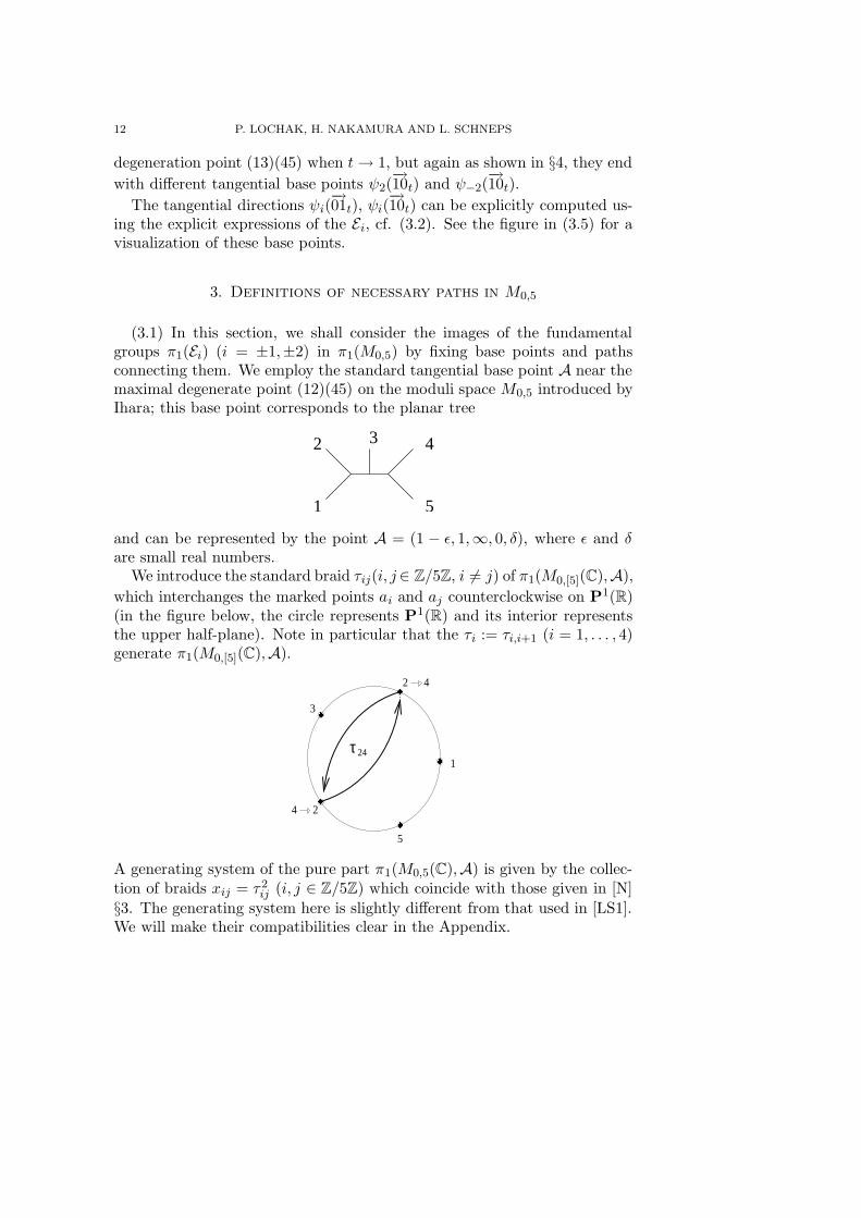
(3.1) In this section, we shall consider the images of the fundamentalgroups π1(Ei) (i = ±1,±2) in π1(M0,5) by fixing base points and pathsconnecting them. We employ the standard tangential base point A near themaximal degenerate point (12)(45) on the moduli space M0,5 introduced byIhara; this base point corresponds to the planar tree

1

3 42

5

and can be represented by the point A = (1 − ε, 1,∞, 0, δ), where ε and δare small real numbers.

We introduce the standard braid τij(i, j∈ Z/5Z, i 6= j) of π1(M0,[5](C),A),

which interchanges the marked points ai and aj counterclockwise on P1(R)(in the figure below, the circle represents P1(R) and its interior representsthe upper half-plane). Note in particular that the τi := τi,i+1 (i = 1, . . . , 4)generate π1(M0,[5](C),A).

τ 241

3

5

2

24

4

A generating system of the pure part π1(M0,5(C),A) is given by the collec-tion of braids xij = τ2

ij (i, j ∈ Z/5Z) which coincide with those given in [N]

§3. The generating system here is slightly different from that used in [LS1].We will make their compatibilities clear in the Appendix.


(3.2) The points of maximal degeneration listed in the table of §2 arecyclically transformed into each other by applications of the automorphism

ρ = (14253) ∈ Aut(M0,5).

The point of maximal degeneration (12)(45) and its images under ρ lie onthe rim of the real 2-dimensional “pentagonal” region of M0,5 consisting ofthe points corresponding to spheres (P1; a1, . . . , a5) with a1, . . . , a5 lying onR ∪ ∞ in that cyclic order. The 5-cyclic point Q1 = (1, ζ, ζ2, ζ3, ζ4) liesin the center of this pentagon.

Letting v1 be the unique (up to homotopy) path from A to Q1 lying inthis simply connected pentagon, conjugating by v1 gives an isomorphismof π1(M0,5, Q1) with π1(M0,5,A). As a movement of points on the sphere(actually sliding without crossing along the real axis), ‘the’ path v1 fromA to Q1 is illustrated in the left-hand figure below. In this figure and allthe following ones, the circle can be viewed either as the unit circle or asthe real axis P1(R) on P1(C), seen from the north pole. Either way, P1(C)equipped with the marked points shown on the circle corresponds to thesame tangential base point or 5-cycle) point on M0,5. Now, because Q1 is aspecial orbifold point of M0,[5], when we wish to consider the image of v1 asa path of the fundamental groupoid in the sense of stacks, we need to choosea tangential direction from which v1 approaches Q1. We take a “shortening”

v1 of the path v1, connecting A to the tangential base point ψ1(−→01t) at Q1,

as illustrated in the right-hand figure below.

12

3

4

5v v1 112

3

4

5

Since the other 5-cyclic point Q2 does not lie in the pentagon, we do not havea canonical choice of a path from A to Q2 = (ζ2, 1, ζ3, ζ, ζ4). We choose suchpath v2 given by motion of points on P1 as in the left-hand figure below,and also a “shortening” v−2 which starts at A and tangentially approaches

the point Q2 in the direction ψ−2(−→01t).


51

2

3

v

45

12

3

v2

4

−2

Further descriptions of v1 and v−2 will be given in the proof of Lemma (3.4).

(3.3) At this stage, we review the definition of kσ(xij) ∈ Γ50 for σ ∈ GQ

which was introduced in [LS2] by the Galois transforms of the path v1 in thefundamental groupoid of M0,5. In this paper we employ another system ofconvention for paths and generators (cf. Appendix), so the definition looksslightly different from the original one in [LS2]. Firstly, if σ fixes the pointQ1 (i.e. if λσ ≡ ±1 mod 5), then we define kσ by

σ(v1) = kσ(xij)−1 · v1.

Next, if σ maps Q1 to Q2 (i.e. if λσ ≡ ±2 mod 5), then σ(v1) is a pro-pathfrom A to Q2. So in this case, we define kσ by

σ(v1) = kσ(xij)−1 · v2.

Now, we shall check that these kσ satisfy property (III′) of Theorem 1.In the case λσ ≡ ±1 mod 5, it is a simple consequence of applying σ tothe homotopy equivalence p = v1ρ(v1)

−1, where we recall that ρ is theautomorphism (14253) ∈ S5 of M0,5, ρ = ρ∗, and p denotes the standardpath (edge of the pentagon) from A to ρ(A). Indeed, we have

fσ(x12, x23) = p σ(p)−1 = pρ(σ(v1))σ(v1)−1 = pρ(k−1

σ )p−1kσ = ρ(kσ)−1kσ .

Similarly, applying σ to p = v1ρ(v1)−1 when λσ ≡ ±2 mod 5 leads to

fσ(x12, x23) = ρ(kσ)−1(pρ(v2)v

−12 )kσ.

It remains only to identify the loop pρ(v2)v−12 as an element of Γ5

0 =π1(M0,5(C),A). Using the definition-drawing of v2 given in (3.2), but draw-ing it “kinematically” as a braid moving downward with time, we find thefollowing illustration of p, followed by ρ(v2) followed by v−1

2 (cf. [LS2] p.592):


p

35 4 2 1

ρ( )

2v

v2

−1

(A)ρ

Q2

A

A

This braid is easily seen to be x25x45 = x34x−115 x45x

−112 . Thus, for all σ ∈ GQ,

our kσ(xij) satisfies the same property (III′) of Theorem 1 as the originalkσ of [LS2].

We next compute the Galois action on the path v1.

Lemma (3.4). There exists a unique path s1 (resp. s2) from ψ1(−→01t) to

ψ−1(−→01t) (resp. ψ−2(

−→01t) to ψ2(

−→01t)) such that, for σ ∈ GQ, we have

σ(v1) =

k−1σ v1 (λσ ≡ 1 mod 5);

k−1σ v1s1 (λσ ≡ −1 mod 5);

k−1σ v−2 (λσ ≡ −2 mod 5);

k−1σ v−2s2 (λσ ≡ 2 mod 5).

Proof. Introduce affine coordinates u, v of the structure ring of M0,5

by (0, u, 1, v−1 ,∞) ∈ M0,5. Then, on the locus near ψi(−→01t) on Ei (i ∈

±1,±2 = (Z/5Z)×), these are expanded as u = ai + tfi(t), v = bi + tgi(t)in the ring Q(ζ)[[t]], where ai, bi ∈ Q(

√5), fi(t), gi(t) ∈ Q(

√5)[[t]]. For each

i, the homomorphism

Q(√

5)[[u− ai, v − bi]] −→ Q(ζ)[[t]] :

u− ai 7→ tfi(t),

v − bi 7→ tgi(t)

determines the location of ψi(−→01t) near the local ring of Q1 or Q2 according

to i = ±1 or ±2. We then have a path li from the Q(√

5)-rational point

Q1 or Q2 to the Q(ζ)-rational tangential base point ψi(−→01t) as the one cor-

responding to the specialization homomorphism Q(ζ)[[t]] → Q(ζ) (t 7→ 0)for each i ∈ (Z/5Z)×. From this definition, one sees that σ(li) = lλσi for


σ ∈ GQ. The paths v1 and v−2 described in (3.2) are then formally definedby v1 := v1 · l1, v−2 = v2 · l−2. Thus, for λσ ≡ ±1, we have

σ(v1) = σ(v1)σ(l1) = k−1σ v1lλσ

,

and for λσ ≡ ±2, we have

σ(v1) = σ(v1)σ(l1) = k−1σ v2lλσ

.

Thus, setting s1 := l−11 · l−1 and s2 := l −1

−2 · l2 give the desired properties.

With regard to the above lemma, we make the following

Definition (3.5). Set v−1 := v1s1, v2 := v−2s2, so that

σ(v1) = k−1σ vi where i ≡ λσ mod 5.

The paths v1, v−1, v2, v−2, s1, s2, l1, l−1, l2, l−2, as well as the four

paths ψi(q) with each of their tangential endpoints ψi(−→01t) and ψi(

−→10t), are

shown in the following figure, which gives a visualization of the identitiess1 = l−1

1 l−1, s2 = l−1−2l2, v−1 = v1s1, v2 = v−2s2 etc.

(12)(45)

A

(10 )t

(10 )t

(13)(45)(10 )t

(10 )t

(01 )t(01 )t (01 )t(01 )t

Q Q

v

v

v1

v−2

2

_

_

_

_

1 21l l2

s1s2

ψ−2

ψ−1

ψ21

ψ

ψ2(q)

ψ−1 ψ

2−2ψψ

1

−2ll−1−1

(q)1

ψ(q)

−2ψψ

−1 (q)

(3.6) The images of the paths v1, v−1, v2, v−2 on the unordered stack

M0,[5] are four different paths from A to the same endpoint ψ( 14

−→01u); by

composing with the infinitesimal path inn(ψ(δ1)) of (2.4), we consider them

as paths from A to ψ(−→01u) (without adding further notation). They induce


four different homomorphisms of (orbifold) fundamental groups

π1(Lu,−→01u) −→ π1(M0,[5],A) (i = ±1,±2)

via γ 7→ viψ(γ)v−1i , where ψ : π1(Lu,

−→01u) → π1(M0,[5], ψ(

−→01u)) is as defined

in (2.4). We are particularly interested in the braids associated to the images

ψ(xu) and ψ(yu) of the generators xu and yu of π1(Lu,−→01u); i.e. we want to

identify the braids associated to the elements

xu,i := vi ψ(xu) v−1i , yu,i := vi ψ(yu) v

−1i (i = ±1,±2)

of π1(M0,[5], ψ(−→01u)) ' Γ

[5]0 .

Proposition (3.7). The table below shows how to identify xu,i, yu,i as braids

in Γ[5]0 .

i | 1 −1 −2 2

xu,i | ϑ3 εϑ3ε V]ϑ3V]

−1 V]εϑ3εV]

−1

yu,i | τ13τ45 ετ13τ45ε V]τ13τ45V]−1 V]ετ13τ45εV]

−1

where ϑ = τ1τ2τ3τ4, V] = τ−14 τ−1

2 τ−13 ϑ2, ε = τ1τ2τ1τ

−14 as in Lemma (1.1).

Proof. In all of the cases to be proved, we work by lifting the loops xu andyu in Lu to paths xt and yt on Lt and then map these paths to M0,5 viaψi and conjugate the results by v1 and v2. This gives paths in M0,5 whichmap down to loops on M0,[5]; by “kinematic” parametrization, we are ableto determine these paths explicitly.

We approximate the small loop xu by the parametrization ε e2πis withs ∈ [0, 1] for very small real ε. This means that upstairs in the space Lt,the parameter t runs through one-fifth of the little circle, which we call xt;it can be parametrized on Lt by t = εζs, s ∈ [0, 1].

The path yu in Lu lifts to the path yt on Lt given in the following figure:

L

Lu

ty

yu

t

Let us begin with xu,1. The image of the little one-fifth circle xt in Ltmaps under ψ1 to

(ζ4 + ζ−4+sε, 1 + ζsε, ζ + ζ−1+sε, ζ2 + ζ−2+sε, ζ3 + ζ−3+sε

)

in E1 ⊂M0,5. For the purpose of visualization, we multiply each componentby ζ2s, which does not change the point in moduli space; for each s ∈ [0, 1],


the same point is now given by(ζ4+2s+ζ−4+3sε, ζ2s+ζ3sε, ζ1+2s+ζ−1+3sε, ζ2+2s+ζ−2+3sε, ζ3+2s+ζ−3+3sε

).

Drawing the motion of each of the five points on the sphere as s varies from0 to 1 yields the left-hand picture of ψ1(xt); we read off from the figure thatthis braid is simply ϑ3. To compute xu,1, this braid must be conjugatedby the path v1 pictured in (3.2). Viewed as a braid, this path consists insliding the points of the tangential base point A apart from each other to atangential base point at the 5-cycle point Q1, so composing by it does notchange the braid (right-hand figure); therefore we obtain xu,1 = ϑ3.

v1−1

v11

23

4 5 s=0

s=1

123

4 5

x(x )ψ u,1(x )ψ1 1t t

For i = −1, 2,−2, we proceed similarly. For xu,−1 (resp. xu,−2, xu,2) weagain parametrize the one-fifth circle xt by t = εζs, plug this into the ex-pression for E−1 (resp. E−2, E2) and multiply the result by ζ2s exactly as fori = 1; the resulting braids, conjugated by v1 and v2 respectively, are shownin the following figure.

v2 v2

v2−1

v2−1

s=0

s=1

x

s=0

s=1

u,−1

−1

x

s=0

s=1

x

(x ) (x )(x )−1

ψ

v1

v1

u,2 u,−2

2ψ

−2ψt t t

123

54

54

3

12

12

3

54

We read the desired braids directly off from this figure. First, clearly xu,−1 =ϑ2; note that this is equal to the expression εϑ3ε given in the statement ofthe proposition, since ε2 = 1 and εϑε = ϑ−1 by Lemma 1.1 (2) and (3).Next, as v2 is identified with the braid τ−1

4 τ−12 τ−1

3 (see the lower half of the

figure in (3.2)) and V] = τ−14 τ−1

2 τ−13 ϑ2, we obtain xu,−2 = V]ϑ

3V −1] and


xu,2 = V]ϑ2V −1

] = V]εϑ3εV −1

] . This completes the proof of the first line of

the table.We use a similar procedure for the yu,i, except that it is actually easier

as no reparametrization is needed. Let us begin with i = 1. The path yt inLt maps into M0,5 as in the following figure; the left-hand side shows it asmovements of points on the sphere, and the right-hand side as the middlesection of a braid, which is conjugated by v1. In the right-hand figure, wehave not drawn the points exactly where they should lie with respect to theequator, i.e. very near the equidistant points of Q1; we have shifted thema little towards the back, so as to be able to read off more easily that thebraid yu,1 is exactly τ13τ45 = τ4τ

−11 τ2τ1.

1

2

3

4

5

u,1y

s=0

s=1

1v

v1

ψ(y )

−1

54

32

1

1 t

It remains to compute yu,−1, yu,−2 and yu,2. For yu,−1, the movement ofpoints and the braid (conjugated by v1) representing ψ−1(yt) are as follows:

s=0

s=1

1v

2

1

3

5

4

45

3 21

yu,−1(y )ψ−1

v−11

t

We read directly off the right-hand figure that yu,−1 is given by τ4τ1τ2τ−11 .

But since ε = τ−14 τ1τ2τ1 and τ2τ

21 τ2τ

21 = τ2

4 , we see that

yu,−1 = εyu,1ε = ετ13τ45ε,

as in the table. For yu,−2 and yu,2, we proceed similarly, but taking careto conjugate by v2 rather than v1; the figures corresponding to ψ−2(yt) and


ψ2(yt) are as follows:

s=0

s=1

(y )

54

32

1

t2

1

53

4

y

v2

ψ−2

v−1

2

u,−2

from which, recalling that V] = τ−14 τ−1

2 τ−13 ϑ2 and noting that ϑ2τ13τ45ϑ

−2 =τ12τ35, we read off

yu,−2 = τ−14 τ−1

2 τ−13 τ12τ35τ3τ2τ4 = V]τ13τ45V

−1] ,

and

s=0

s=1

v

2

45

3 21

y(y )ψ

v−1

t

1

53

4

2

2

2

u,2

from which we read off

yu,2 = τ−14 τ−1

2 τ−13 τ−1

4 τ3τ4τ1τ3τ2τ4.

However, for the middle part of the braid, we have

ψ2(yt) = τ−14 τ3τ4τ1 = τ3τ4τ

−13 τ1 = ϑ2τ1τ2τ

−11 τ4ϑ

−2,

and thus,

yu,2 = V]τ1τ2τ−11 τ4V

−1] = V]ετ

−1τ2τ1τ4εV−1] = V]ετ13τ45εV

−1]

by a simple computation of braids using ε = τ1τ2τ1τ−14 and the identity

τ1τ22 τ1τ

22 = τ2

4 . This concludes the proof of the proposition.


4. Local factors at the tangential base points

(4.1) In this section, we shall look closely at the tangential base points

ψi(−→10t) (i = ±1,±2) near the maximal degenerate point (13)(45). We shall

take a standard tangential base point B near the point (13)(45) given by the

ring of Puiseux series Qq1, q2 :=⋃

′

N Q[[q1/N1 , q

1/N2 ]] (cf. [IN]), where the

coordinates q1, q2 are defined by

(a1, a2, a3, a4, a5) ∼ (q−12 , 1,∞, 0, q1).

Here ∼ means the equivalence of tuples by fractional transformations ofP1. We shall identify the tangent space at the maximal degenerate point(13)(45) on M0,5 with C2 by the coordinates (q1, q2). The tangential basepoint B is equivalent to that given by the tangent vector (1, 1) ∈ C2.

First, one can compute the case ψ1(−→10t) as follows.

(ζ4 + ζ−4t, 1 + t, ζ + ζ−1t, ζ2 + ζ−2t, ζ3 + ζ−3t

)

∼(

1

U(1 − t)(1 +O(1 − t)

) , 1,∞, 0, V (1 − t)(1 +O(1 − t)

)),

where

U =5

(1 − ζ)5= −

(1 +

√5

2

)5/2

5−1/4i,

V =5

(1 − ζ2)5=

(1 +

√5

2

)−5/2

5−1/4i,

and 1 +O(1− t) designates some power series in Q(ζ)((1− t)) with constantterm 1.

Since the other tangential base points ψi(−→10t) (i = −1,±2) are Galois

conjugates of ψ1(−→10t), the corresponding tangent vectors are easy to identify.

We list the coordinates of the corresponding tangent vectors in the followingtable:

| ψ1(−→10t) ψ−1(

−→10t) ψ2(

−→10t) ψ−2(

−→10t)

q1 | V −V −U U

q2 | U −U V −V

(4.2) We shall connect these tangent vectors (V,U), (−V,−U), (−U, V ),(U,−V ) with (1, 1) by the straight lines on C2. These lines give (etale


homotopy) paths

r1 : ψ1(−→10t) → B,

r−1 : ψ−1(−→10t) → B,

r2 : ψ2(−→10t) → B,

r−2 : ψ−2(−→10t) → B

on M0,5/Q. These paths determine specialization homomorphisms of

Qq1, q2 to Q1 − t via the principal branches of roots N√V , N

√U ,

N√−U , N

√−V nearest to 1. For example, r1 represents the homomorphism

sending q1/N1 , q

1/N2 to N

√V (1− t)1/N , N

√U(1− t)1/N respectively. The Galois

transformation of r1 is then given by the following

Lemma (4.3). For j = 1, 2, let Xj ∈ π1(M0,5,B) be the path corresponding

to the local monodromy q1/nj 7→ ζ−1

n q1/nj (n ≥ 1, ζn = exp(2πi/n)). For

σ ∈ GQ, define the values ρV (σ), ρU (σ) ∈ Z by the Kummer property alongthe principal (i.e., nearest to 1) branches of n-th roots of V and U :

σ( n√V )

n√σ(V )

= ζρV (σ)n ,

σ( n√U)

n√σ(U)

= ζρU (σ)n (n ≥ 1).

Then, we have

σ(r1) = ri ·X−ρV (σ)1 X

−ρU (σ)2 (σ ∈ GQ),

where i ∈ ±1,±2 is determined by the condition i ≡ λσ mod 5.

Proof. Put σ(r1) = σ · r1 · σ−1 = ri · Xc11 X

c22 and apply both sides to the

functions q1/n1 separately. The left-hand side gives then ζ

ρV (σ)n (σ(V ))1/n(1−

t)1/n, while the right-hand side gives ζ−c1n (σ(V )(1 − t))1/n. This concludes

c1 = −ρV (σ). The same argument for q1/n2 determines the value of c2.

(4.4) Set X1,i := (viψi(q)ri)(X1)(vψi(q)ri)

−1,

X2,i := (viψi(q)ri)(X2)(vψi(q)ri)−1

to be the loops based at A obtained by conjugating the loops X1 and X2,based at B, by the paths viψi(q)ri from A to B. Then, in a similar way to(3.6), we have the following expression of X1,i by braids in π1(M0,5,A):

i | 1 −1 −2 2

X1,i | x45 εx45ε V]x45V]−1 V]εx45εV]

−1

X2,i | x13 εx13ε V]x13V]−1 V]εx13εV]

−1


We note that ε commutes with τ4 and hence with x45. Comparing the tablein (3.6), we note that

y2u,i = X1,iX2,i (i = ±1,±2).

Before closing this section, we shall relate the above ρU , ρV with thefunctions χ13, χ45 introduced in §1.

Lemma (4.5). As Z-valued functions on GQ, we have

χ13 =

2(ρ5 − ρ2 − ρU ) +

0, (λ ≡ 1 mod 5)

−1 (λ ≡ −1 mod 5)

2(ρ5 − ρ2 − ρV ) +

0, (λ ≡ −2 mod 5)

−1 (λ ≡ 2 mod 5)

χ45 =

2(ρ5 − ρ2 − ρV ) +

0, (λ ≡ 1 mod 5)

1 (λ ≡ −1 mod 5)

2(ρ5 − ρ2 − ρU ) +

1 (λ ≡ −2 mod 5),

0 (λ ≡ 2 mod 5)

Proof. The proof is obtained from case-by-case examination of the branchesof n-th roots of quantities and of Galois actions on them. We treat the casewhere λσ ≡ −2 mod 5. In this case, one has

σ( n√U)

n√V

=σ( n

√U)

n√

−σ(U)= ζ

ρU (σ)− 1

2n .

This implies

σ( n√u)

n√v

= ζρ5−ρ2−ρU+ 1

2n

for all n ≥ 1, hence, χ45 = 2(ρ5 − ρ2 − ρU ) + 1. We leave it to the reader tocheck the other cases.

5. Path deformations and proof of Theorem A

(5.1) Recall that q is the path from−→01 to

−→10 on Lt, and ψ1 : Lt → E1 ⊂

M0,5. Thus, ψ1(q) is its image on M0,5. We shall homotopically deform thepath ψ1(q) so as to run near to the maximal degenerate point (12)(45) as

follows. The starting point of ψ1(q) is a the tangential base point ψ1(−→01t)

neighboring the point t = 0 in E1, which we can normalize as follows:

Q1 = (1

−ζ2 − ζ3, 1,∞, 0,

1

1 − ζ2 − ζ3) ∼ (0.6, 1,∞, 0, 0.4).


The endpoint of ψ1(q) is the tangential base point ψ1(−→10t) given by

(1/ε, 1,∞, 0, δ) (for small positive real numbers ε and δ) neighboring themaximally degenerate point (∞, 1,∞, 0, 0), i.e. (13)(45). Represented onthe sphere with marked points, the parametrized path ψ1(q) is as follows:

0.6 1 0 0.48We see in this figure that the path ends at a tangential base point whichis not one of the standard (real) ones. We deform it to a homotopic pathdrawn as

0.6 1 0 0.48

1 2 3 4 5

We can undo this path into three parts as follows:

0.6 0.4

1−ε δ

qq2 11 8 0

081

1 8 0

" V "

c a

r

12

v

"U "

1

-1

-1

-1

-1

1-1

The first part is exactly the path v−11 ; it starts at the starting point of ψ(q),

namely at the tangential base point ψ(−→01t) near the 5-cycle point Q1, and


ends at the tangential base point represented by A = (1 − ε, 1,∞, 0, δ) forsmall positive real numbers ε and δ, neighboring the maximally degeneratepoint (12)(45). The second part takes place in the neighborhood of infinityof the moduli space, and consists in the commutativity move c−1

12 (a right halftwist, see for example [NS]), taking the point to (1, 1 + ε,∞, 0, δ) numbered(2, 1, 3, 4, 5), followed by the associativity move a = a21,13 which brings thispoint to B ∼ (1/ε, 1,∞, 0, δ) simply by sliding the second point along thereal axis from ε to 1/ε; the point B is a tangential base point near (13)(45).The third part is a local path around (13)(45) going from B to the tangential

base point ψ1(−→10t), which by construction is exactly the path r−1

1 of (4.2).Thus we obtain the decomposition

(5.2) ψ1(q) = v−11 · c−1

12 · a · r−11 .

We now come to the proof of the main result of this article.

(5.3) Proof of Theorem A : By (5.2), we have an equivalence of paths

v1 · ψ1(q) · r1 = c−112 · a

from A to B. On the right-hand side, the Galois action on those paths alongthe 1-dimensional strata at infinity in M0,5 are well-known (cf. [NS]) andmay be calculated as:

(5.4) σ(c−112 a) = x

1−λσ2

12 f(x12, x13)−1 · c−1

12 a

for σ ∈ GQ. To consider Galois transformations of the left-hand side, fixσ ∈ GQ and take i ∈ ±1,±2 so that i ≡ λσ mod 5. Recall that by Lemma(2.5), we have

σ(πi(ψ1(q))

)= ψ(xu)

−2ρ2f(ψ(xu), ψ(yu)

)−1ψ(yu)

2ρ5−2ρ2 πi(ψi(q)

).

Using this (and dropping the πi from the notation, as it is merely an inclusionof groups), together with Definition (3.5) and Lemma (4.3), we find that theGalois transformation of the left-hand side can be given as:

σ(v1 · ψ1(q) · r1) = kσ(xij)−1vi · ψ(xu)−2ρ2f

(ψ(xu), ψ(yu)

)−1(5.5)

· ψ(yu)2ρ5−2ρ2 · ψi(q) · ri ·X−ρV (σ)

1 X−ρU (σ)2

= σ(c−112 a)

= x1−λσ

2

12 f(x13, x12)c−112 a

Summing up, we obtain

(5.6) kσ(xij) = FiX−ρV (σ)1,i X

−ρU (σ)2,i Sif(x12, x13)x

λσ−1

2

12 ,


with

Fi : = vi · ψ(xu)−2ρ2f

(ψ(yu), ψ(xu)

)ψ(yu)

2ρ5−2ρ2 · v−1i ,

X1,i : = (vi · ψi(q)ri)(X1)(viψi(q)ri)−1,

X2,i : = (vi · ψi(q)ri)(X2)(viψi(q)ri)−1,

Si : = vi · ψi(q) · ri · a−1c12.

Given that Fi is exactly equal to

Fi = x−2ρ2u,i f(yu,i, xu,i)y

2ρ5−2ρ2u,i ,

we find, using the table of Proposition (3.6) and the identities f(ετ13τ45ε, ϑ2)

= εf(τ13τ45, ϑ3)ε and ε2 = 1, that

Fi =

ϑ−6ρ2f(τ13τ45, ϑ3)(τ13τ45)

2ρ5−2ρ2 (i = 1),

ϑ6ρ2εf(τ13τ45, ϑ3)(τ13τ45)

2ρ5−2ρ2ε (i = −1),

V]ϑ−6ρ2f(τ13τ45, ϑ

3)(τ13τ45)2ρ5−2ρ2V]

−1 (i = −2),

V]ϑ6ρ2εf(τ13τ45, ϑ

3)(τ13τ45)2ρ5−2ρ2εV]

−1 (i = 2).

In other words, for λ = λσ and heavily using Lemma (1.1) (2), (3) and (4)(especially for λ ≡ ±2), we have

(5.7) Fi = Vλελϑ−6ρ2λ f(τ13τ45, ϑ

3λ) ·

(τ13τ45)2ρ5−2ρ2 (i = 1),

(τ13τ45)2ρ5−2ρ2ε (i = −1),

ε′(τ13τ45)2ρ5−2ρ2V]

−1 (i = −2),

ε′(τ13τ45)2ρ5−2ρ2εV]

−1 (i = 2).

Now, using the table in (4.4), we have

(5.8) X−ρV

1,i X−ρU

2,i =

τ−2ρU

13 τ−2ρV

45 (i = 1),

ετ−2ρU

13 τ−2ρV

45 ε (i = −1),

V]τ−2ρU

13 τ−2ρV

45 V]−1 (i = −2),

V]ετ−2ρU

13 τ−2ρV

45 εV]−1 (i = 2).

It remains to compute the Si. Since ψ1(q) = v−11 c−1

12 a r−11 , we see that

S1 = 1. In fact, we can treat all of the Si, i = ±1,±2 simultaneously bydrawing the paths ψi(q)ri with certain components normalized to 0, 1, ∞


and proceeding as for i = 1:

3

1

2

4

5

3

1

5

4

3

2

15

4

3

2

1

5

Ψ2 2(q)r−2

(q)r−2Ψ

−1(q)r

−1(q)r

1 ΨΨ1

4

2

From this drawing of ψ−1(q), we see that it is homotopic to v−11 c12a r

−1−1;

thus, S−1 = c12 · c12 = x12. For i = ±2, we compute Si by composing thepictured paths as braids, starting with v2 (drawn in (3.2)), as follows:

1234

5

1

352

4

1234

5

1

352

4

S2

v

−1

2 2

−1

v−2

−2(q)r

−2

a c12

(q)r

2

Ψ Ψ

S−2

a c 12

We read the braids immediately from this picture:

S−2 = τ−14 τ−1

2 τ−13 τ4τ3ϑ

−1τ1, S2 = τ−14 τ−1

2 τ−13 τ−1

4 τ−13 ϑ−1τ1.

Using simple braid relations, one can rewrite these expressions using theimportant involutive braid ε′ = τ2ϑ

2τ1 (see Lemma (1.1)) which exchanges


τ13 and τ45 by conjugation. We obtain:

(5.9) Si =

1, (i = 1),

x12, (i = −1),

V]τ13ε′, (i = −2),

V]ετ−145 ε

′, (i = 2).

This, together with (3.2) and (5.4), after being collected into (5.5), reducesthe proof of Theorem A to checking

τχ13

13 τχ45

45 =

xρ5−ρ2−ρU

13 xρ5−ρ2−ρV

45 ·

1 (λ ≡ 1 mod 5),

τ−113 τ45 (λ ≡ −1 mod 5),

xρ5−ρ2−ρU

45 xρ5−ρ2−ρV

13 ·τ45 (λ ≡ −2 mod 5),

τ−113 (λ ≡ 2 mod 5).

But this follows from Lemma (4.5). The proof of theorem A is thus com-pleted.

(5.10) In this subsection, we discuss how to extend the functions χ13, χ45

of §1 fromGQ to GT by using Ihara’s theory [I2]. We assume basic propertiesof the profinite free differential calculus. Consider the partial derivative∂fσ(x,y)

∂y in the complete group algebra Z[[F2]] for σ ∈ GT , and write its

image in Z[x]/(x5 − 1) (with y = 1) as:

(5.10.1)∂fσ(x, y)

∂y≡ −

4∑

a=0

κa5(σ)x−a mod (x5 − 1).

This formula defines the extension to GT of the coefficients κa5 which appearas the Soule characters in the case where σ ∈ GQ. Indeed, by [I2], we know

that κ05 = −ρ5 on GQ ⊂ GT and

(5.10.2) ζκa5(σ)

n =

σ

(n

√1 − ζλ

−1σ a

n

)

n√

1 − ζan(n ≥ 1, σ ∈ GQ)

for a = ±1,±2. Therefore, to extend χ13, χ45 to GT , it suffices to express

them in terms of κa5’s (together with ρ2 whose extension to GT was discussedin [LNS], [NS]). This can be done by looking closely at branches of roots.

In fact, we obtain the following equations of Z-valued functions on GQ for


which we omit to describe the detailed case-by-case examinations :

χ13 + 2ρ2 =

10κ15 + 2λ− 2 (λ ≡ 1 mod 5),

10κ15 − λ− 2 (λ ≡ −1 mod 5),

10κ15 − 2 (λ ≡ −2 mod 5),

10κ15 − λ− 2 (λ ≡ 2 mod 5),

(5.10.3)

χ45 + 2ρ2 =

10κ25 (λ ≡ 1 mod 5),

10κ25 − λ (λ ≡ −1 mod 5),

10κ25 − λ (λ ≡ −2 mod 5),

10κ25 + 2λ (λ ≡ 2 mod 5).

(5.10.4)

The meaning of this extension is that the equality in theorem A, which holdswhenever (λσ, fσ) is associated to an element of GQ, can now be posited as

a relation on elements of GT , which may or may not be satisfied by all

elements of GT .

6. Interpretation of results and some prospects

We have thus completed the proofs of theorems A,B. In this section,we will add a few remarks about their overall meaning, especially in theframework of Grothendieck-Teichmuller theory. Eigenloci can be defined ingeneral in the moduli stacks Mg,n (resp. Mg,[n]) of curves of genus g with nlabeled (resp. unlabeled) marked points; their main defining property is tobe stable (though not necessarily pointwise fixed, of course) under the actionof a finite subgroup of the modular group Γng (resp. Γng ) corresponding tothe automorphism group of some algebraic curve (see [L] for more detail).

Here we have used a very special case, namely a rational eigencurve E(dimension 1 eigenlocus) in M0,5. Apart from the two key properties of Ementioned in the Introduction, namely that E is stable under the actionof ρ and that its image in M0,[5] is a copy of P1 with a missing pointand two orbifold points, we have actually used a third geometric property,namely that E intersects the divisor at infinity ofM0,[5] at a point of maximal

degeneration. The equation of E = E (5) can immediately be generalized toany n. Just write the same formula as in (2.3) above with ζ a primitive n-throot of unity and n entries of the form zi(t) = ζ i+ ζ−it, i = 0, 1, . . . , n. The

corresponding eigencurve E (n) ⊂ M0,n still enjoys the two key properties,but the third fails for n ≥ 5, a point to which we will briefly return below.

Let us briefly show that the method we used in this paper could have beenused in the lower dimensions n = 3, 4 in order to compute the elements gσand hσ in terms of fσ as was done in Theorem 2 of the Introduction); it turnsout that the method and the result is essentially similar to what was done in


[NT]. First, we mention an easy fact, true for general n, which is implicitlyused below in the case n = 3. One can mark not just the n points zi(t) onthe sphere, but also one or both of the points 0 and/or ∞; these are the tworamification points of the rotational symmetry of order n given by t 7→ ζnt.Adding in one or both of these distinguished points defines eigencurves inM0,n+1 and M0,n+2 whose automorphism groups decrease accordingly; forinstance, adding in the point ∞ decreases the automorphism group from adihedral group to a cyclic group, as the additional symmetry t 7→ 1/t nolonger preserves the set of marked points.

Let us proceed to gσ and hσ. Write z = (z1, z2, z3, z4) for a point on M0,4

and use the following definition of the cross-ratio:

[z1, z2, z3, z4] =z2 − z1z3 − z1

× z3 − z4z2 − z4

,

so that z ∼ (0, z, 1,∞) where ∼ is equivalence under the PGL2 action andz = [z1, z2, z3, z4]. Recall that θ (resp. ω) denotes the order 2 (resp. 3)automorphism of P1 \ 0, 1,∞ given by z 7→ 1 − z (resp. z 7→ 1/(1 − z)).Take n = 4, and let us study the order 2 symmetry θ.

The eigencurve E (4) parametrized by t reads:

(6.1) z(t) = (1 + t, i− it,−1 − t,−i+ it).

Putting this into the standard cross-ratio form (0, z(t), 1,∞) as above, wefind that

(6.2) z(t) =1

2− it

1 − t2.

There are four values of t for which the corresponding point of E (4) isdegenerate, namely t = ±1,±i. The corresponding points on M0,4 arez(1) = z(−1) = ∞, z(i) = 1 and z(−i) = 0, so the image of the locus

E (4) (minus the degenerate points) in M0,4 simply coincides with M0,4. Thepermutation group S4 acts on M0,4 via S3 = S4/V , where V is the group ofproducts of disjoint transpositions, which does not act effectively; the groupS3 is seen as permuting the points 0, 1 and ∞. Applying the 4-cycle (1234)

to E (4), we find that it acts via the involution t 7→ −t (its square belongs toV ), so that it acts on z(t) via z(−t) = 1 − z(t) = θ(z(t)). Moreover, thetransformation t 7→ 1/t induces the transposition (24), and acts on z(t) viaz(1/t) = z(−t) = θ(z(t)). This means that the whole order 8 dihedral sub-group D4 ⊂ S4 generated by the 4-cycle (1234) and the transposition (24)(compare with the case n = 5 in §2.1) projects to a group of order 2 in S3

corresponding to the subgroup of the automorphisms of the line generatedby θ.

Because E (4) coincides with M0,4, its stabilizer coincides with the wholeof S3. Yet, by analogy with the case n = 5 (actually any n ≥ 5), and


following the above, it is natural to single out the group generated by θ asthe ‘meaningful’ stabilizer. Mimicking the construction in §2.1, one thenintroduces the u-line with u = β(t) = 4t(1 − t), which is a Belyi functiondescribing the invariants under θ. We are now precisely in the situation of[NT] (§4) which produces equation (GF1) of Theorem 2 in the Introduction.In turn, equation (GF0) of that same theorem is obtained using the wholeof S3 as the stabilizer (which it is!) and the attending invariants.

The case of hσ , with n = 3, can be treated much in the same way. Let ξdenote a primitive third root of unity, and parametrize the eigenlocus E (3)

as follows:

(6.3) z(t) = (1 + t, ξ + ξ2t, ξ2 + ξt,∞),

where the point ∞ is added as explained above, so as to work in the non-trivial moduli space M0,4 rather than the trivial space M0,3. In normalizedform one gets:

(6.4) z(t) = −ξ 1 − ξ2t

1 − ξt.

The points t = 0,∞ give the two points of order three, and t 7→ ξ2t corre-sponds to the action of ω: we have z(ξ2t) = ω(z(t)). One also computesthat z(1/t) = 1/z(t), corresponding to the transposition (23) of the points 0

and ∞. This time the dihedral group D3 ⊂ S4 associated with E (3) projectsto the whole of S3, and following the same procedure, one is led to look at anorder 6 cover describing the S3 invariants, as in [NT] (§3), that is to equation(HF0) of Theorem 2. Equation (HF1) is derived by taking an intermediatecover of order 3, corresponding to the invariants under the 3-cycle ([NT],§5). Logically speaking, in order to retrieve this last equation, one could add

the point 0 in the definition of E (3), getting a curve in M0,5 with a stabilizercyclic of order 3, because the involution t 7→ 1/t does not apply anymore.However one then has to compute in the fundamental group of M0,[5], whichis fairly artificial here.

We thus find that the consideration of the eigencurves E (3) and E (4) leadsto a computation of the parameters gσ and hσ in the Galois case, in termsof fσ, which essentially coincide with the computations of [NT] given in

Theorem 2. The present paper has been devoted to E (5) and the computationof kσ . To summarize, one can say that it completes the computation of theGalois action on the automorphisms at the first two levels in terms of theaction on the groupoid at infinity. Indeed, g, h and k describe the action ofthe Galois group on the automorphism groups of the curves on the modulispaces of dimensions 1 and 2. (This could and should be made a little moreprecise, as we have considered only the genus 0 spaces (M0,[4] and M0,[5])here, but in fact the genus 1 spaces (M1,1 and M1,[2]) are similar to the genus


0 spaces, and in particular are uniformized by the same complex Teichmullerspaces.) As for f , it describes the action on the groupoid at infinity of M0,4,which is enough to describe the action at infinity on all the spaces Mg,n andMg,[n], based at the ‘standard tangential points’.

The elements gσ, hσ and kσ carry explicit information about the action of

GT on certain torsion elements of the mapping class groups. At present, not

much is known about the GT (resp. GQ) action on such elements; in general,what can be said is as follows (cf. [S], [L]). Because we are considering the

GT action (and not the outer action), the choice of base point is important:here, we take the standard tangential base point at infinity.

Armed with some material on stacks and their fundamental groups, it isnot difficult to prove the following general result (see [LV]): Let γ be a finiteorder diffeomorphism of a topological surface of type (g, [n]), corresponding

to a torsion element γ ∈ Γ[n]g (with the same name). One associates with the

conjugacy class of the cyclic group 〈γ〉 a nonempty closed integral substackMγ of the Q-stack Mg,[n], called the special locus of γ, whose closed pointscorrespond to algebraic curves having an automorphism which acts topolog-ically like γ. This locus Mγ is defined over a finite extension k = k(γ) of Q

(where one needs to be a little careful about the notion of field of definition;a formal way to put it is that the (coarse) moduli space associated to theresidual gerbe of the generic point of Mγ is isomorphic to Spec(k)). Theresult then says that for σ ∈ Gk, σ preserves the conjugacy class of γ. Thisis a completely general fact, coming from the behavior of stack inertia underthe Galois action.

In this context, one can view the work in [NT] and the present paper ascomputing the conjugating factors of the finite order elements η = τ1τ2τ1,

ξ = τ1τ2 in Γ[4]0 and ϑ = τ1τ2τ3τ4 in Γ

[5]0 under the GQ-action. Namely, for

all σ ∈ GQ, we have

η 7−→ τ−4ρ21 f(η, τ2

1 ) · ηλ · f(τ21 , η)τ

4ρ21 ;(6.5.1)

ξ 7−→ τ1−λ

2−3ρ3

1 f(ξ, τ21 ) · ξλ · f(τ2

1 , ξ)τ3ρ3+λ−1

2

1 ;(6.5.2)

ϑ 7−→ x1−λ

2

12 f(x13, x12)τ−χ45

45 τ−χ13

13 f(ϑ3λ, τ13τ45)(6.5.3)

· ϑλλ · f(τ13τ45, ϑ3λ)τ

χ45

45 τχ13

13 f(x12, x13)xλ−1

2

12 ,

where η = τ1τ2τ1, ξ = τ1τ2 ∈ B3 and ϑ = τ1τ2τ3τ4 ∈ Γ[5]0 . See §1, Lemma

(1.1)(3) for recalling ϑλ.Proof. Since (6.5.1-2) are easier, we only prove (6.5.3) here. First note thata lift of ϑ3 on M0,5 gives the standard path from A to ρ(A). Therefore, one


can comupute σ(ϑ3) after Theorem 1 (III′) and Lemma (1.1)(1) as follows:

σ(ϑ3) = f(x12, x23)−1ϑ3

=

k−1ϑ3k, (λ ≡ ±1 mod 5),

k−1V]ϑ4V −1

] k (λ ≡ ±2 mod 5),

=

k−1ϑ3λk (λ ≡ 1 mod 5),

k−1εϑ3λεk (λ ≡ −1 mod 5),

k−1V]ϑ3λV −1

] k (λ ≡ −2 mod 5),

k−1V]εϑ3λεV −1

] k (λ ≡ 2 mod 5).

This together with Lemma (1.1)(4) and Theorem A computes the conjugat-ing factor of ϑ3λ

λ in σ(ϑ3). As ϑ = (ϑ3)2, the conjugating factor of ϑ λλ inσ(ϑ) is the same.

These hold for the Galois action, but what about the GT -action? Wehave less information in this case; we only know that the following precise

version of the above conjugacy result holds in genus 0 for all σ ∈ GT : σ(γ)

is a conjugate of γχ(σ) for all finite-order γ ∈ Γn0 (in genus 0, the field ofdefinition k is cyclotomic). It turns out (see [S]) that in a sense we will notexplain here, the information contained in the automorphisms in genus 0is enough to recover the information at infinity in all genera. Note againthat it is not known whether the relations in [NT] and the present paperconnecting g, h and k with f (as well as those involving f only, such as in

Theorems 3 and B) are satisfied in the original version of GT (defined in[Dr], see also [F]).

7. Appendix: Dictionary of conventions for paths and

generators

In this Appendix, we introduce the “σ-convention” and the “τ -conven-tion”, each of which consists of a coherent set of rules on path composition,

braid generator systems and associated definitions of GT -parameters. Bothconventions have been used in recent papers on Grothendieck-Teichmullertheory, and the present paper is based on the τ -convention. We give a recipefor translating formulas into each other so that the reader will be equippedto easily read papers written in either convention.

[σ-convention]: Paths are composed from right to left. If γ1 is a pathfrom A to B and γ2 is a path from B to C, then γ2γ1 denotes the composedpath from A to C. Paths act on functions on the left. If γ is a path fromA to B, and if f is a germ of functions defined near A, then γ(f) meansthe germ of functions near B analytically continued along γ. We call this


the monodromy action of γ. If c is a small counterclockwise loop around0 of the affine t-line A1(C), then c(t1/n) = ζnt

1/n. Given an etale coverφ : Y → X and a path γ on X from x0 to x1, then γ induces a bijection γ :φ−1(x0) → φ−1(x1). In the monodromy action, we have (γγ ′)(∗) = γ(γ ′(∗)).The standard generators x,y, z of π1(P

1 − 0, 1,∞,−→01) with xyz = 1 aretaken as follows: x is a small counterclockwise loop around 0; y is a looprunning along the real segment [0,1], turning counterclockwise around 1 andrunning back along the real segment; z is a loop running mainly on the lowerhemisphere and turning counterclockwise around ∞. Defining p as the path

from−→01 to

−→10, we introduce the non-commutative proword fσ(∗, ∗) by the

equation in π1(P1 − 0, 1,∞,−→01): σ(p) = pfσ(x,y) for σ ∈ GQ. Pick n

points ai = ζin (i ∈ Z/nZ) on P1(C) ∼= S2. The standard generator systemσij |1 ≤ i 6= j ≤ n of the sphere braid group on a1, . . . , an is taken so thatσij interchanges ai and aj counterclockwise on the lower hemisphere. It iswritten by the minimal standard generators as

σij = σ−1i · · · σ−1

j−1σjσj−1 · · · σi (1 ≤ i < j ≤ n).

Here, braids, like paths, are composed from right to left, and drawn onstrands numbered from left to right, with σi denoting the braid in whichthe i-th strand crosses to the right over the (i+ 1)-st strand. We define thepure braid xij := σ2

ij; the elements σ24 and σ4 are shown as a movement ofpoints and a braid in the following figure.

1

2 4

4

5

2

σ24

3

3 42 51

σ24

1 2 3 4 5

σ4

[τ -convention]: Paths are composed from left to right. If γ1 is a path fromA to B and γ2 is a path from B to C, then γ1γ2 denotes the composed pathfrom A to C. Paths act on functions on the left. If γ is a path from A to B,and if f is a germ of functions defined near B, then γ(f) means the germ offunctions nearA analytically continued along γ. We call this the monodromyaction of γ. If c is a small counterclockwise loop around 0 of the affine t-lineA1(C), then c(t1/n) = ζ−1

n t1/n. Given an etale cover φ : Y → X and a path γonX from x0 to x1, then γ induces a bijection γ : φ−1(x1) → φ−1(x0). In themonodromy action, we have (γγ ′)(∗) = γ(γ ′(∗)). The standard generators

x, y, z of π1(P1−0, 1,∞,−→01) with xyz = 1 are taken as follows: x is a small

counterclockwise loop around 0; y is a loop running along the real segment


[0,1] and turning counterclockwise around 1; z is a loop running mainly onthe upper hemisphere and turning counterclockwise around ∞. Defining p as

the path from−→01 to

−→10, we introduce the non-commutative proword fσ(∗, ∗)

by the equation in π1(P1 − 0, 1,∞,−→01): σ(p) = fσ(x, y)

−1p for σ ∈ GQ.The standard generator system τij |1 ≤ i 6= j ≤ n of the sphere braidgroup on the above a1, . . . , an ⊂ P1(C) is taken so that τij interchangesai and aj counterclockwise on the upper hemisphere. It is written by theminimal standard generators as:

τij = τ−1i · · · τ−1

j−1τjτj−1 · · · τi (1 ≤ i < j ≤ n).

Note here that the braids are composed from left to right, and drawn onstrands numbered from right to left, with the generator τi crossing the i-thstrand to the left under the (i + 1)-st strand. We define the pure braidxij := τ2

ij, and draw τ24 and τ4 below.

τ 241

3

5

2

24

4 12345

τ24

3

4τ

15 24

Dictionary. We produce a dictionary between the above two conventions.Our principle is to identify paths as monodromy operators on germs of func-tions (i.e. we consider pictures of braids or loops only as “superficial expres-sions” within each convention, and do not base our convention translationson them). This helps us from extra-cares on reversing multiplication ordersin translations, by virtue of the above definitions of monodromy in bothconventions. So, p = p−1, x = x−1, y = y−1 while z = yz−1y−1. Then, forσ ∈ GQ, σ(p) = pfσ(x,y) is equal to σ(p−1) = p−1fσ(x, y) = pfσ(x

−1,y−1).

Therefore, as prowords of two non-commutative generators X,Y of F2, wehave

fσ(X,Y ) = fσ(X−1, Y −1).

It is obvious that the GT -relation (I) for fσ is equivalent to that for fσ. On

the other hand, the equivalence of the GT -relation (II) for fσ and that for fσis a(n easy but) non-trivial exercise. We leave it for interested readers. The

equivalence of the GT -relation (III) for both conventions can be assuredfrom the translation of braids as monodromy operators: σi = τ−1

i . This


gives, in general,

σij = xi,i+1 · · · xi,j−1τ−1ij x

−1i,j−1 · · · x−1

i,i+1,

τij = x−1i,i+1 · · · x−1

i,j−1σ−1ij xi,j−1 · · ·xi,i+1

for 1 ≤ i < j ≤ n. Under the above translation rule, we have, for example,

fσ(x12,x23) = fσ(x−112 ,x

−123 ) = fσ(x12, x23).

Thus, GT -equations in the sphere braid groups look same in both conven-tions, as long as they involve only f -parameters and braid generators ontwo consecutive strings. The relation (III) is a case in point. But recently,

more complicated equations have been studied in the theory of GT , whichinvolve more general types of generators or local factors with Kummer typecharacters as exponents. To illustrate the situation, let us consider Theo-rem A of this paper, for the case λ ≡ 1 mod 5 for simplicity. Then, in theτ -convention, it reads:

kσ(xij) = ϑ−6ρ2f(τ13τ45, ϑ3)τχ13

13 τχ45

45 f(x12, x13)xλ−1

2

12 .

where kσ(xij) is defined by σ(v) = kσ(xij)−1v for a certain path v fromA to Q. The corresponding kσ should be defined by σ(v) = vkσ(xij) usingv = v−1. Then, kσ(x12,x23,x34,x45,x51) = kσ(x12, x23, x34, x45, x51). Thetranslation then gives us

kσ(xij) = ϑ−6ρ2fσ(x−112 σ13σ45x12,ϑ

2)x−112 σ

−χ13

13 σ−χ45

45 fσ(x12,x13)x3−λ

2

12

where ϑ = σ1σ2σ3σ4 = τ−11 τ−1

2 τ−13 τ−1

4 = τ1τ2τ3τ4 = ϑ.

References

[Dr] V.G. Drinfeld, On quasitriangular quasi-Hopf algebras and a group closely con-

nected with Gal(Q/Q), Leningrad Math. J. 2(4) (1991), 829–860.[F] H. Furusho, Geometric and arithmetic subgroups of the Grothendieck-Teich-

muller group, Math. Res. Lett. 10 (2003), 97–108.[G] A. Grothendieck, Esquisse d’un Programme, 1984, in “Geometric Galois Ac-

tions I”, P.Lochak, L.Schneps (eds.), London Math. Soc. Lect. Note Ser. 242(1997), 5–48.

[I1] Y. Ihara, On the embedding of Gal(Q/Q) into GT∧, in “The Grothendieck theoryof Dessin’s d’Enfants”, L.Schneps (ed.), London Math. Soc. Lect. Note Ser. 200,(1994), 289–306.

[I2] Y. Ihara, On beta and gamma functions associated with the Grothendieck-Teich-

muller group modular group, in “Aspects of Galois Theory”, H. Voelklein et.al(eds.), London Math. Soc. Lect. Note Ser. 256 (1999), 144–179; Part II, J. ReineAngew. Math. 527 (2000), 1-11.

[IM] Y. Ihara, M. Matsumoto, On Galois actions on profinite completions of braid

groups, in “Recent Developments in the Inverse Galois Problem”, M. Fried et.al.(eds.), (1995), 173–200.


[L] P. Lochak, On arithmetic curves in the moduli spaces of curves, preprint 2002.[LNS] P. Lochak, H. Nakamura, L. Schneps, On a new version of the Grothendieck-

Teichmuller group, Note aux C.R.A.S., Serie I 325 (1997), 11–16.[LS1] P. Lochak, L. Schneps, Grothendieck-Teichmuller group and automorphisms

of braid groups, in “The Grothendieck theory of Dessin’s d’Enfants”, L.Schneps(ed.), London Math. Soc. Lect. Note Ser. 200 (1994), 323–358.

[LS2] P. Lochak and L. Schneps, A cohomological interpretation of the Grothendieck-

Teichmuller group, Invent. Math. 127 (1997), 571–600.[LV] P. Lochak and M. Vaquie, in preparation.[N] H. Nakamura, Galois rigidity of pure sphere braid groups and profinite calculus,

J. Math. Sci. Univ. Tokyo 1 (1994), 71–136.[N-I,II] H. Nakamura, Limits of Galois representations in fundamental groups along

maximal degeneration of marked curves, I, Amer. J. Math. 121 (1999), 315–358;Part II, Proc. Symp. Pure Math. 70 (2002), 43–78.

[NS] H. Nakamura, L. Schneps, On a subgroup of the Grothendieck-Teichmuller

group acting on the tower of profinite Teichmuller modular groups, Invent. Math.141 (2000), 503–560.

[NT] H. Nakamura, H. Tsunogai, Harmonic and equianharmonic equations in the

Grothendieck-Teichmuller group, Forum Math. 15 (2003), 877–892.[S] L. Schneps, Automorphisms of curves and their role in Grothendieck-Teichmuller

theory, preprint 2003.[T] H. Tsunogai, Some new-type equations in the Grothendieck-Teichmuller group

arising from geometry on M0,5, preprint 2003.

Pierre Lochak

Institut de Mathematique de Jussieu,

175 rue de Chevaleret, F-75013 Paris, France

e-mail address: [email protected]

Hiroaki Nakamura

Department of Mathematics, Okayama University,

Okayama 700-8530, Japan


Leila Schneps

Institut de Mathematique de Jussieu,

175 rue de Chevaleret, F-75013 Paris, France


(Received January 28, 2004 )

Documents

EIGENLOCI OF 5 POINT CONFIGURATIONS ON THE …webusers.imj-prg.fr/~leila.schneps/LNS.pdf · Math. J. Okayama Univ. YY(20XX), xxx{yyy EIGENLOCI OF 5 POINT CONFIGURATIONS ON THE RIEMANN