Efficient Auction Mechanisms for Supply ChainProcurement

Rachel R. Chen*, Robin Roundy**Rachel Q. Zhang*, and Ganesh Janakiraman**

* Johnson Graduate School of Management, Cornell University,Ithaca, NY 14853

** Department of Operations Research and Industrial Engineering,Cornell University, Ithaca, NY 14853

Abstract

We consider multi-unit Vickrey auctions for procurement in supply chain settings.This is the first paper that incorporates transportation costs into auctions in a complexsupply network. We introduce three incentive compatible auction mechanisms. Two ofthem make simultaneous production and transportation decisions so that the supplychain is cost-efficient for the quantities awarded to the buyer, and the third determinesthe production quantities before the shipments. We show that considerable supplychain cost savings can be achieved if production and transportation costs are consideredsimultaneously. However, under the typical regular-overtime production cost structure,the buyer’s payments in efficient auctions can be high so that the buyer may preferinefficient auction protocols. We develop an efficient auction that can control the sizeof the buyer’s payments at the expense of introducing uncertainty in the quantityacquired in the auction.

1 Introduction

Research and practice in operations management has emphasized integrated supply chains,where long-term relationships between suppliers and buyers of manufactured componentsfacilitate optimization of total supply chain costs. There is a recent emphasis on usingauctions in the supply chain as an effective and efficient means of achieving lower acquisitioncosts, lower barriers for new suppliers to enter a market, and consequently better marketefficiency. Exploiting recent advances in information technology, such auctions can be carriedout through the Internet, referred to as online auctions. Online auctions allow geographicallydiverse buyers and sellers to exchange goods, services, and information, and to dynamically

1

determine prices that reflect the demand and supply at a certain point of time so that efficientmatches of supply and demand can be realized. As pointed out by Lucking-Reiley (2000),online auctions often lead to lower information, transaction and participation costs, as wellas increased convenience for both sellers and buyers, the ability for asynchronous bidding,and easier access to larger markets.Most auctions are price-driven. However, there are other costs associated with inte-

grating a supply chain, e.g., costs associated with transportation, capacity management,inventories, etc. Recently there have been escalating disputes in the electronics industryon fair pricing in supply chains. According to industry executives, OEMs and suppliers areignoring the numerous additional costs that affect parts prices, such as shipping, logistics,and value-added services when they quote prices. They are passing such costs onto theirmanufacturing partners and distributors, squeezing profitability out of the channel (Elec-tronic Business News, 11/19/2001). According to Mike Dennison, senior director of GlobalProcurement and Strategic Supply Chain Management at Flextronics International, “Sup-pliers must understand all the complexities of getting material from their dock to the OEM’sand need to factor in the cost when they are quoting a price”. This issue relates to morethan a general understanding of terms and conditions, according to Andy Fischer, vice pres-ident and channel director for Avnet Electronics Marketing at Avnet Inc., “Continuity (ofa supply chain) . . . is not only channel related, it’s also global. Service packages, demandcurves, global locations all lead to different costs and requirements.” As Chopra and VanMieghem (2000) point out, accounting for these additional costs may be a key issue in B2Bauctions. Yet, there is a lack of decision analysis that combines sophisticated OR/MS toolswith economic insights to help supply chain practitioners in auctions and e-marketplaces(Keskinocak and Tayur 2001).The goals of this paper are to design multi-unit auctions that achieve overall supply chain

efficiency while taking into account production costs and transportation costs that have beenignored in most of the auction literature, and to illustrate some of the risks and tradeoffsassociated with these auctions. For example, in manufacturing systems per-unit costs tendto be relatively flat if the regular-time capacity of the manufacturing system is not exceeded,and to grow rapidly when overtime or other measures are required to increase capacity inthe short term. In an efficient auction, this property of manufacturing cost functions canlead to substantial payments to suppliers. We will see that the buyer may prefer an auctionthat is clearly inefficient for the supply chain, simply because it reduces the size of thesepayments. The buyer can control the size of these payments via a reservation price, at theexpense of new risks associated with the quantity purchased in the auction.The paper is organized as follows. We discuss some of the relevant literature in Section

2, and introduce our models in Section 3. In Sections 4 and 5 we discuss the analyticalproperties of our auction mechanisms. In Sections 5.3 and 6 we discuss payment reductionat the cost of uncertainty in the quantity purchased in the auction, and payment-induceddistortions of buyer behavior, respectively. The paper concludes in Section 7.

2

2 Literature Review

Incorporating transportation costs into production and shipment decisions has been a richresearch area in operations research. As an example, Sharp et al. (1970) consider a manu-facturer who owns multiple production plants with non-linear production costs and providesproducts to multiple demand locations. The demands at different locations are known andthe objective is to minimize the total production and transportation costs. When there ismore than one production facility and production costs are non-linear, the common approach,which combines production and transportation costs on each arc of the supply network andmakes production and transportation decisions based on a single cost function, does notapply. Recently, Holmberg and Tuy (1999) extend the classic transportation problem byallowing fixed costs of production at the supply nodes, and stochastic demand and convexnon-linear penalty costs for being short at the demand centers. They reduce the problemto a simpler optimization problem and solve it using a branch and bound method. Bothpapers provide lists of references dealing with similar optimization problems. However, noneof them considers pricing decisions using auctions.Bidding behavior in auctions has been studied since 1950’s using game theory and decision

theory (Rothkopf 1969). We refer the reader to Vickrey (1961), Milgrom and Weber (1982),Klemperer (1999), McAfee and McMillan (1987), and Rothkopf and Harstad (1994) forclassical auction theory. In a typical auction, there is a single buyer who wants to purchasea single unit or a number of units of a product. There are several potential suppliers (orsellers) in the market; each has her own cost structure. (Since the analysis for the case witha single seller and multiple buyers is the same, we will focus on the case with a single buyerand multiple sellers). To participate in the auction, each supplier is required to submit abid to an auctioneer (also called a market intermediary or an agent). Based on these bids,the quantity to purchase from, and the payment to each supplier, are determined by theauctioneer through pre-specified rules known as a mechanism. A mechanism is incentivecompatible (or induces truth-telling) if each supplier’s dominant strategy is to submit hertrue production cost as her bid. Incentive compatibility is important because it is usually arequirement for an auction to be efficient. An efficient mechanism is one that guarantees anallocation of production quantities that minimizes the total system costs.There are three dominant types of mechanisms for multi-unit auctions, known as Pay-

as-You-Bid, uniform-price, and VCG auctions (e.g. second-price auctions in the single-unitsetting, also known as Vickrey auctions) (Klemperer 1999). The Pay-as-you-Bid auction isself-explanatory. In a uniform auction a uniform price is paid for each unit purchased. Theprice can be either the first rejected or the last accepted bid. In economics literature it iswell known that neither Pay-as-You-Bid nor uniform-price auctions is incentive compatibleor efficient, whereas the family of mechanisms known as VCG auctions, attributed to Vickrey(1961), Clarke (1971), and Groves (1973), are both incentive compatible and efficient. In aVCG auction, the buyer’s payment to a supplier is based not only on the bids submitted,but also on the contribution that the supplier makes to the system by participating in theauction. This payment structure motivates suppliers to improve their operational efficiency

3

and lower their production costs, increasing the contribution they make to the system. Thereader is referred to Nisan and Ronen (2001) for a general definition of the VCG family ofauction mechanisms. In spite of the attractive properties of VCG auctions, they are notwidely used in practice, largely due to the fact that human auctioneers may take advantageof the truth telling bidders and do not always act truthfully (Rothkopf et al. 1990).Recently, we have seen research on auctions from OM’s perspective. Beil and Wein (2001)

consider a manufacturer who uses a reverse auction to award a contract to suppliers basedon both prices and a set of non-price attributes (e.g., quality, lead time). Pinker et al. (2001)design sequential, multi-unit online B2C auctions to allocate a fixed amount of inventory overcertain number of periods. Eso (2001) develops an iterative sealed bid auction (where bidderscan not see others’ bids) for selling excess capacity for an airline company. Vulcano et al.(2001) consider variants of the second-price auction (i.e., the single-unit Vickrey auction) ina multi-period revenue management problem where each individual bidder can be awarded atmost one unit. Jin and Wu (2001) show that auctions can serve as a coordination mechanismfor supply chains.It is noted that most research on auctions limits its effort to either single-unit auctions

or multiple-unit auctions under which each bidder wants at most one unit (Keskinocak andTayur 2001). In this paper, we allow each supplier to be awarded multiple units. Themain contribution of this paper to the OR/MS literature is the integration of productionand transportation costs in multi-unit auctions that involves multiple supplier locations andbuyer locations. Since the auction mechanisms that we propose fall into the VCG family,they are incentive compatible and produce efficient solutions for the supply chain whenproduction and transportation decisions are made simultaneously.As we mentioned above, VCG auctions are rarely used because of possible cheating by

the auctioneer. In an online auction, however, the auctioneer can be a web site (virtualcomputer agent) which receives bids, and decides awards and payments based on some pre-specified algorithm so that this problem can be minimized or eliminated. Furthermore, theinternet may make auctions more secure as bidders may come from all over the world and thealgorithm can be designed not to reveal buyers’ and suppliers’ private information. Rapidadvances in computational capability make it possible to conduct sophisticated allocationrules quickly and at low cost. With the recent advances in information technology, VCGauctions have the potential to become an important mechanism for online auctions. Thisis the first paper that uses the VCG auction mechanism in a complex supply chain settingthat achieves global optimization of both production and transportation costs. This alsoopens the door to the solution of a host of supply chain optimization problems using theseauctions.

3 Model Introduction

Consider a single buyer who has requirements, called consumption quantities, for a certaincomponent at a set of geographically diverse locations. As in the standard auction literature,we assume the buyer has private valuation of the consumption quantities at the demand

4

locations, which form the consumption vector, and she will act strategically to maximize herutility (i.e., her valuation minus her payments). The buyer’s private valuation is given bya consumption utility function representing the dollar value of every possible consumptionvector to the buyer. This could be, for example, the buyer’s expected profit (excludingthe acquisition costs which will be determined by the auction) that a consumption vectorwould bring in. Multiple suppliers, each of whom owns a set of production facilities, areavailable to satisfy these requirements. Every supplier has a production cost, which can bedescribed as a convex function of the quantities that she produces at her production locations.Note that in economics, such a cost can already include a reasonable profit margin of theindustry. We also assume that each supplier is a rational, self-interest player who is tryingto maximize her own profit (i.e. the payment received minus her production cost). Theconvexity of a production cost function implies increasing marginal cost in the quantitiesproduced, which includes the case where the overtime marginal production cost is higherthan the marginal cost during regular production time. With general convex productioncosts, one can not simply combine the production and transportation costs and treat themas a single cost function. In addition, the buyer pays the transportation costs associatedwith every shipment from a supplier location to a buyer location. We assume that thebuyer knows the per-unit transportation cost along each arc of the network, and there is nocoalition among the suppliers, which is reasonable because it is relatively harder for suppliersto form a coalition in online auctions.We consider three auction mechanisms, T , R, and S. All three of them require each

supplier to submit a bid, a function of the quantity supplied by her, representing her desiredprices. Although the three mechanisms have the same payment structure as that of the VCGfamily, they can sometime lead to very different payments.

Auction T : In this auction, the buyer submits a fixed consumption vector, q, to theauctioneer, who will decide the quantities each supply location will provide to eachdemand center by minimizing the system production and transportation cost. Un-der the VCG payment structure, Auction T is incentive compatible and efficient. Weinvestigate how the buyer determines her consumption vector, and show that the con-sumption vector picked by the buyer usually will not optimize the total supply chain(i.e., maximize the total net utility of the buyer and the suppliers). Although AuctionT is incentive compatible and efficient, it may result in unreasonably high paymentsfor the buyer.

Auction R: In this auction, the buyer submits a utility function (a proxy for hertrue consumption utility function) to the auctioneer, rather than a fixed consumptionvector. The auctioneer treats this as if it were the profit (excluding acquisition costs)that the buyer makes by consuming q, a consumption vector, and considers it whenmaking production and transportation decisions. The quantities that the buyer willbe awarded and her payments are the outputs of the auction.

Under the VCG payment structure, Auction R is incentive compatible for the suppliers,but NOT for the buyer. The auction mechanism meets the consumption vector q at

5

minimum production and transportation cost and hence, is efficient for providing q. Italso typically results in a consumption vector q that fails to optimize the total supplychain.

Under Auction R, we show that the buyer’s payments are always less than or equalto those in Auction T for providing the same level of consumption. We derive thebuyer’s optimal strategy assuming the buyer knows the suppliers’ production costs(i.e., under complete information) and show that, in general, the buyer will not submither true consumption utility function. We also consider Auction R under uncertaintyin suppliers’ production costs and investigate how the buyer’s decision on her biddingfunction affects her awarded quantities and payments.

Auction S: To demonstrate the benefits of incorporating transportation costs into auc-tions, we examine Auction S. In Auction S, the buyer submits a fixed consumptionvector to the auctioneer who will decide the production quantities at all supplier lo-cations and the buyer’s payments to the suppliers by minimizing the total productioncost in the system. Transportation decisions are subsequently made to match the de-mand and supply at the lowest total transportation cost. It is obvious that Auction Tachieves a lower total supply chain cost than Auction S. However, the buyer may pre-fer Auction S under certain circumstances. We found that the typical regular-overtimeproduction cost structure can lead to higher payments in efficient auctions to distortbuyer behavior.

Before introducing the detailed auction mechanisms, we define the notation and introduceour first assumption.

N = total number of supplier production facilities

K = number of suppliers

M = total number of buyer locations

Nk = set of production facilities owned by supplier k

kn = index for the supplier that owns production facility n

qm = consumption at demand center m, qm > 0

xn = production quantity at production facility n

ynm = quantity shipped from production facility n to demand center m

zkm =Xn∈Nk

ynm, total quantity shipped to demand center m by supplier k

Ck(xk) = production cost function for supplier k (R|Nk| → R)Fk(xk) = bidding function from supplier k (R|Nk| → R)

τnm = cost for shipping one unit from production facility n to demand center m

We use boldfaced letters to represent vectors or matrices, whose dimension will be clear fromthe context. In particular, xk = (xn : n ∈ Nk) and zk = (zkm : 1 ≤ m ≤M). For simplicity,we use ∂f(x) to denote the set of all subgradients of f(·) at x.

6

Assumption 1 The production cost function Ck(·) and bidding function Fk(·) are non-decreasing convex and closed with Ck(0) = Fk(0) = 0. Furthermore, Ck(·) (Fk(·)) is subdif-ferentiable at points where Ck(·) <∞ (Fk(·) <∞).

4 Auction T

In this section, we study Auction T where the buyer submits a fixed consumption vector qto the auctioneer. Supplier k submits to the auctioneer a bid function Fk(xk) for supplyingxk units, for which she incurs a production cost Ck(xk), xk ∈ R|Nk|. The suppliers may ormay not see the consumption vector.As in any auction, the auctioneer will decide the quantities awarded to each of the

suppliers, the amount transported from each supplier location to each of the buyer locations,and the payments made by the buyer to the sellers. Under Auction T , the auctioneer willminimize the sum of the accepted bids and the transportation costs, for a given consumptionvector q, as

Min.KXk=1

Fk(xk) +NXn=1

MXm=1

τnmynm (4.1)

s.t.NXn=1

ynm = qm, m = 1, . . . ,M ; (4.2)

MXm=1

ynm = xn, n = 1, . . . , N ; (4.3)

ynm ≥ 0, m = 1, . . . ,M, n = 1, . . . , N. (4.4)

Let π(q) be the optimal value of the objective function for a given q. Define Q = {q :q > 0,π(q) <∞} and we restrict q ∈ Q to ensure sufficient supply capacity. Since Fk(·) isclosed, for any q ∈ Q, an optimal solution exists.Let (xT ,yT ) be an optimal solution, and π−k(q) be the optimal value of the objective

function with the additional constraint xk = 0 (i.e., supplier k does not participate in theauction). The buyer will pay supplier k

ψTk (q) = π−k(q)− π(q) + Fk(xTk ) (4.5)

where π−k(q)−π(q) is the bonus payment made to supplier k, representing the value she addsto the system by participating in the auction. The buyer pays supplier k her bid Fk(x

Tk ) plus

her contribution to the system. This payment scheme belongs to the general truth-inducingVCG family described in Nisan and Ronen (2001). Consequently, rational suppliers will bidtheir costs, Fk(xk) = Ck(xk), irrespective of other suppliers’ bids. Therefore, Auction T isincentive compatible for all suppliers (see Vickrey (1961), Clarke (1971) and Groves (1973))and π(q) =

PKk=1Ck(x

Tk ) +

PNn=1

PMm=1 τnmy

Tnm, the minimum total supply chain cost for

meeting the demand q. That is, truth-telling implies that Auction T is efficient.

7

The total cost incurred by the buyer, κ(q), is her total payments to the suppliers plusthe transportation costs, i.e.,

κ(q) =KXk=1

ψTk (q) +NXn=1

MXm=1

τnmyTnm =

KXk=1

π−k(q)− (K − 1) · π(q). (4.6)

4.1 Basic properties of Auction T

Here we list several properties of Auction T that will be used repeatedly in the subsequentsections.

Property 1 π(q) and π−k(q) are increasing convex functions of q.

Property 1 follows directly from the convexity of the production cost functions and lin-earity of the transportation costs in the convex program (4.1) — (4.4).

Property 2 For any optimal solution (xT ,yT ) for a given q ∈ Q, there exist nonnegativeLagrange multipliers, v ∈ RM and u ∈ RN associated with constraints (4.2) and (4.3), suchthat the following results hold.

1. uk ∈ ∂Ck(xTk ) for all k.2. vm = un+τnm if ynm > 0 and vm ≤ un+τnm if ynm = 0. That is, vm = min

1≤n≤N{un+τnm}

for all m.

3. v ∈ ∂π(q) and v ∈ ∂π−k(q− zTk ) where zTkm =P

n∈Nk

yTnm, 1 ≤ m ≤M .

The proof of Property 2 can be found in the Appendix. To understand Property 2, considerthe case where π(·), π−k(·) and Ck(·) are differentiable. Then the first two results in Property2 become

un =∂Ckn(x

Tkn)

∂xn,

∂Ckn(xTkn)

∂xn+ τnm =

∂π(q)

∂qm, for yTnm > 0,

∂Ckn(xTkn)

∂xn+ τnm ≥ ∂π(q)

∂qm, for yTnm = 0.

That is, suppliers who supply demand center m do so with the same marginal production-plus-transportation cost, and suppliers who do not supply demand center m have largermarginal costs at demand location m. The third result, v = ∇π(q) = ∇π−k(q − zTk ),implies that the marginal supply chain cost remains the same if we take supplier k andher allocation, zTk , out of the system. These results establish the relationships between themarginal production and transportation costs at any supply location and demand center,

8

and the relationships between the marginal costs at any demand center with and without asupplier (and her bids).Since v may not be unique in general, we define V (q) as the set of all v that satisfy

Property 2. That is, V (q) = {v : ∃ some u such that (u,v) satisfies Property 2 for some(xT ,yT ) given q ∈ Q}. Note that V (q) is nonempty and only depends on q.

Property 3 For any optimal solution (xT ,yT ) for a given q ∈ Q, there exists (xT−k,yT−k)representing an optimal solution without supplier k such that yT−knm (q − zTk ) = yTnm for 1 ≤m ≤M and n∈Nk, and xT−kk0 (q−zTk ) = xTk0 for k0 6= k. That is, if we take supplier k and herawarded quantities zTk out of the system, then the production and transportation quantitiesat other suppliers in the auction with fixed demand q − zTk remain the same. Furthermore,π−k(q− zTk ) is the minimum cost for providing q− zTk without supplier k, and

π(q) = π−k(q− zTk ) + Ck(xTk ) +Xn∈Nk

MXm=1

τnmyTnm. (4.7)

The proof for Property 2 is straightforward and hence, omitted here.

4.2 The Buyer’s Choice of q

We now discuss how the buyer determines her consumption vector q in auction T and howher decision deviates from the one that optimizes the total supply chain. Assume thatthere exists a Consumption Utility Function, U(q), that specifies the profit (excluding theacquisition costs that will be determined by the auction) the buyer will make by consuming q.The buyer will choose the consumption vector qB that maximizes her net utility U(q)−κ(q).This differs from qA, the consumption vector that optimizes supply chain by maximizing thetotal net utility of the buyer and the suppliers, U(q) − π(q). As κ(q) ≥ π(q), one mightexpect qB ≤ qA. This is true when M = 1, but may not always be true for M > 1 as thefollowing example illustrates.Consider a system with 2 suppliers (K = 2). Each owns a single production facility

(N = 2) with production costs C1(x) = C2(x) = x2. The buyer has 2 demand centers(M = 2) with consumption utility function U(q1, q2) = 30, 000 − 3[100 − (q1 + q2)]2 ifq1 + q2 ≤ 100 and U(q1, q2) = 30, 000 otherwise. That is, there is zero utility associatedwith each additional unit above 100. Unit transportation costs are τ11 = τ21 = τ12 = 1,and τ22 = ∞. This implies that yT22 = 0 for all q. Furthermore qB2 = 0 because, if qB2 > 0,then when supplier 1 is removed from the auction, the buyer’s transportation cost would beinfinite. Thus the buyer would have to make an infinite payment to supplier 1. Consequently,to maximize the buyer’s net utility U(q1, q2) − κ(q1, q2), the buyer will choose q

B2 = 0 and

yB12 = 0. This leads to

π(q1, 0) = q21/2 + q1,

π−1(q1, 0) = π−2(q1, 0) = q21 + q1.

9

Consequently the buyer’s net utility is

U(qB1 , 0)− κ(qB1 , 0) = maxn30, 000− 3(100− q1)2 − (3q21/2 + q1)

o.

The solution is (qB1 , qB2 ) = (66.6, 0).

By contrast, total supply chain costs are minimized by solving

U(qA)− π(qA) = max 30, 000− 3[100− (q1 + q2)]2−[(y11 + y12)2 + y221 + y11 + y12 + y21]

s.t. y11 + y21 = q1,

y12 = q2.

The result is (qA1 , qA2 ) = (64.17, 21.3), and q

B1 > q

A1 .

Although a VCG type auction is incentive compatible and efficient for any given q, aspointed out by Ausubel and Cramton (1998), such an auction can be very expensive forthe buyer. Consider 10 identical suppliers who meet a total demand of 90 units at a singledemand center. Assume that transportation costs are negligible. At each supplier location,C(x) = F (x) = x for x ≤ 9 and 9 + 100(x − 9) for x > 9. Then it is optimal for allsuppliers to produce 9 units at $1.00 each and π(90) = $90. If we remove one supplierfrom the system, the rest of the suppliers will have to produce 9 more units at $100 each,which leads to π−k(90) = $981 for all k. The payments from the buyer are then given byψk = π−k(90) − π(90) + C(9) = $900 for all 10 suppliers. So the buyer pays a total of$9, 000 versus the real production cost of $90. The reason for such a high payment is that,when capacity is tight and production costs are sharply convex for some suppliers, the totalproduction costs may be significantly different when one of these suppliers is taken out ofthe system. The bonus payment can be very large, even for something produced at very lowcosts.Another potential problem with Auction T is that when bidders are asymmetric, i.e.,

some suppliers have relatively high capacity, removing a supplier with large capacity mayresult in insufficient capacity and an infinite π−k(q) value.

5 Auction R

In this section, we propose a new auction mechanism, Auction R, that will result in muchlower payments for the buyer and yet still induces the suppliers to bid their true costs.In this auction, the buyer submits a function W (q) as a proxy for her true consumptionutility, U(q), rather than a fixed consumption vector as in Auction T . W (q) is treated bythe auctioneer as if it were the profit (excluding acquisition costs) that the buyer makesby consuming q. We refer to W (·) as the buyer’s bidding strategy and make the followingassumption about U(·) and W (·).Assumption 2 U(q) and W (q) are increasing concave and closed with U(0) = 0 andW (0) = 0. Furthermore, U(·) (W (·)) is subdifferentiable at points where U(·) <∞ (W (·) <∞).

10

As we will see, by submitting W (q) the buyer is actually reporting a reservation pricefunction for each unit she might acquire. It is well-known that one’s true reservation price forany unit is the first derivative of her true consumption utility function and is usually NOTidentical for all units. Instead, it may well be a decreasing function of the number of units onealready has on hand. While in most auctions, the payment made to a supplier is determinedby bids from all sellers, in Auction R, part or all of the payments will be determined by thebuyer’s reservation price. This prevents the buyer from making unreasonable payments.The auctioneer solves the optimization problem min{π(q) − W (q)} to determine an

optimal consumption vector qR and associated production quantities xR and shipments yR.If there are multiple minimizers, we assume that the auctioneer will always choose an optimalconsumption vector qR with the maximum total purchase quantity.

Let qR−kbe the solution to min{π−k(q)−W (q)}, Π(W ) = π(qR)−W (qR) and Π−k(W ) =

π−k(qR−k)−W (qR−k). Following the VCG payment structure, the payment made to supplierk is

ψRk (W ) = Π−k(W )− Π(W ) + Fk(xRk ). (5.8)

5.1 Properties of Auction R

In this section, we show that under (5.8), the suppliers will still bid their costs Ck(·), andthe buyer pays less for purchasing qR in Auction R than in auction T . We first introducethe following assumption.

Assumption 3 There exists a finite consumption vector qmax such that W (q) =W (q1, .., q

maxm , .., qM) if qm > q

maxm − 1 for all q, for W (·) satisfying Assumption 2. That is,

the buyer associates no utility to any consumption in excess of qmaxm − 1 at demand centerm, 1 ≤ m ≤M .

Assumption 3 guarantees that qR < qmax.

Theorem 1 Under assumption 3, truth-telling is the dominant strategy for all suppliers inauction R.

We show that Theorem 1 holds by establishing that Auction R is equivalent to a T typeauction. Consider a T type auction with fixed consumption vector qmax and the buyer as anadditional supplier. The buyer has a production facility with ample capacity co-located witheach demand center. These production facilities can only supply their own demand centersand the transportation costs are naturally zero. The buyer is required to bid as a supplierand will bid the following convex function that satisfies Assumption 1,

FB(x) =

0, if xm < 0 for some m,W (qmax)−W (qmax − x), if 0 ≤ x ≤ qmax,+∞, otherwise,

11

where x represents the vector of the buyer’s production quantities. The auctioneer will thensolve min

0≤x≤qmax{π(qmax−x)+W (qmax)−W (qmax−x)} or min

0≤q≤qmax{π(q)+W (qmax)−W (q)},

which is equivalent to min0≤q≤qmax{π(q)−W (q)}. That is, this T type auction with fixed demand

vector qmax and an additional dummy supplier is equivalent to the original Auction R.In this equivalent T auction, the real suppliers will provide the actual consumption vector

qR and the dummy supplier, which has enough capacity at each demand center, will supplythe remaining xRB = qmax − qR. The amounts the real suppliers will produce and ship tothe demand locations, and the actual payments to the real suppliers are exactly the same asthose resulting from Auction R. The existence of a dummy supplier does not affect suppliers’behavior in the equivalent T auction and, as a result, all suppliers will bid at their productioncosts.As we can see, Auction R has the following nice properties. (i) It is still incentive

compatible for the suppliers. (ii) By Theorem 1, π(qR) =PKk=1Ck(x

Rk )+

PNn=1

PMm=1 τnmy

Rnm

is the minimum total system cost given qR. Hence, (xR,yR) minimizes the total supplychain cost for producing and shipping qR.If the buyer also submits her true consumption function U(q), Auction R will maximize

U(q)− π(q) and optimize the total supply chain. Interestingly, it is usually not optimal forthe buyer to do so, as we will show in the next section when we discuss the buyer’s optimalbidding strategy. The buyer will usually manipulateW (·) to gain some control over the totalacquisition cost

κR(W ) =KXk=1

ψRk (W ) +NXn=1

MXm=1

τnm · yRnm =KXk=1

Π−k(W )−K ·Π(W ) + π(qR).

Since qR−kminimizes {π−k(q)−W (q)},

W (qR)− π−k(qR) ≤ W (qR−k)− π−k(qR

−k)

for all k. Consequently

κT (qR)− κR(W ) =

KXk=1

nW (qR

−k)− π−k(qR

−k)−

hW (qR)− π−k(qR)

io≥ 0,

and we have the following theorem.

Theorem 2 Let qR be a consumption vector that results from W (q) that the buyer submitsin Auction R. The buyer will pay more to purchase the same quantity, qR, in Auction T .That is, κR(W ) ≤ κT (q

R).

From Theorem 2, it appears that the buyer should prefer Auction R to Auction T .However as we will see subsequently, Auction T has an important advantage. If the buyerdoes not have complete information about the suppliers’ production costs, she cannot predictqR in advance. The degree of uncertainty in the quantity acquired favors Auction T .

12

5.2 The Buyer’s Optimal Bidding Strategy

We now explore the optimal W (q) that the buyer would submit with complete informationunder Auction R. We first derive lower bounds for the buyer’s total payment κR(W ) for agiven concave functionW (q). We then show that there exists a concave functionW ∗(q) suchthat κR(W

∗) is at the best lower bound and the buyer’s profit U(q)− κR(W ) is maximized.To establish the lower bounds for the buyer’s total payment, we first introduce the followinglemma.

Lemma 3 For any optimal solution (xR,yR,qR) in auction R for a given W (·) satisfyingAssumption 3, there exist nonnegative Lagrange multipliers v ∈ RM , u ∈ RN and uB ∈ RM

that satisfy the following.

1. uk ∈ ∂Ck(xRk ) for all k and uB ∈ ∂FB(xRB).2. By Assumption 3, xRB > 0. Since the dummy production facilities only supply theirown demand centers, xRB = yRB and v = uB. If we let rm = min

1≤n≤N{un + τnm}, then

rm = vm = uBm if qRm > 0 and rm ≥ vm = uBm if qRm = 0.

3. r ∈ ∂W (qR), r ∈ ∂π(qR), and r ∈ ∂π−k(qR − zRk ).The proof of Lemma 3 is in the Appendix. Lemma 3 indicates that, ifW (·), π(·), and π−k(·)are differentiable, then the marginal utility equals to the marginal supply chain cost withand without supplier k at an optimal solution qR and qR − zRk . Since r may not be uniquefor any qR, let γ(W,qR) be the set of all r defined in Lemma 3. That is, γ(W,qR) = {r :r is defined in Lemma 3 for some (xR,yR,qR)}. We are now ready to establish the lowerbounds of the buyer’s total payment for given W (·).

Lemma 4 For any function W (·) satisfying Assumption 3 and the resulting qR in AuctionR, κR(W ) ≥ r · qR, for any r ∈ γ(W,qR).

The proof of Lemma 4 is in the Appendix. We now show that if Ck(·) is strictly increasingfor all k, there exists W (q) such that the buyer’s payment κR(W ) is at one of the lowerbounds. Bidding at this function, the buyer will pay a uniform price for all the unitspurchased at the same demand location.Let Γ(q) = {r : r ∈ γ(W,qR) for some W (·) satisfying Assumption 3 and resulting in

qR = q}. Then for any r ∈ Γ(q), r ∈ ∂π(q), r ∈ ∂π−k(q − zRk ), and r ∈ ∂W (q) for someW (·) by Lemma 3.

Lemma 5 Assume that Ck(·) is strictly increasing for all k. Pick any q ∈ RM , and any rfrom Γ(q). If the buyer submits W (q) =

PMm=1min{qm, qm} · rm in Auction R, the resulting

consumption vector is qR = q and the buyer’s total payment is κR(W ) = r · q. That is, thebuyer pays a uniform price rm for all qm units shipped to demand center m.

13

The proof of Lemma 5 is in the Appendix. We now derive the buyer’s strategy W ∗(·) thatmaximizes her net utility U(qR) − κR(W ). As you will see, the structure of W

∗(·) has thesame form as that in Lemma 5 and the buyer needs to find the (q, r) pair, r ∈ Γ(q), thatmaximizes {U(q)− r ·q}. For a given q, let r∗(q) ∈ Γ(q) maximize {U(q)− r ·q}. Also, letq∗ maximize {U(q)− r∗(q) · q} and r∗ = r∗(q∗).Theorem 6 The optimal function the buyer should submit is W ∗(q) =

PMm=1min{qm, q∗m} ·

r∗m.

The proof of Theorem 6 is in the Appendix. By Theorem 6, the buyer’s optimal strategy isdetermined by two parameters, (r∗,q∗). To find r∗, we need to identify the set Γ(q). As youwill see in the following lemma, Γ(q) is actually equal to the set V (q) defined in Section 3.1and hence, is nonempty and only dependent on q.

Lemma 7 Γ(q) = V (q), for any q ∈ Q.The proof of Lemma 7 is in the Appendix. If π(q) is differentiable for q ∈ Q, then Γ(q) =∇π(q) and we can solve for the optimal q∗ by maximizing {U(q) −∇π(q) · q}. Otherwisewe can use a differentiable function to approximate π(q) and solve for q∗ approximately.With the buyer’s optimal strategy specified, we can consider the example in Section 3

with 10 identical suppliers under Auction R. In that example, the total buyer’s paymentfor providing 90 units under Auction T is $9, 000 while the total production cost is only$90. Recall that there is only one demand center so we can ignore the subscript m. Tomake a meaningful comparison, we assume that q∗ = 90. Then the optimal r∗ = $1.00,which is the marginal supply chain cost at q∗ = 90, and W ∗(q) = min(q, q∗)r∗. Furthermore,q∗R = q∗ = 90, z∗Rk = 9, q∗R − z∗Rk = 81, π(q∗R) = $90, and π−k(q∗R−k) = $81 for all k. Sothe buyer’s total payment is given by

κR(W∗) =

10Xk=1

[π−k(q∗R−k)−W ∗(q∗R−k)]−10Xk=1

[π(q∗R)−W ∗(q∗R)] + π(q∗R)

=10Xk=1

[W ∗(90)−W ∗(81)] +10Xk=1

[π−k(81)− π(90)] + π(90) = 90

which happens to be the minimum supply chain cost.Interestingly, when the buyer submits her optimal bidding function, W ∗(q), she actually

pays a uniform price r∗m for all the units shipped to demand center m. This uniform priceis her submitted reservation price, as W ∗(q) is her submitted consumption utility. If π(·)is differentiable, r∗m =

∂π(q∗R)∂qm

, the marginal supply chain cost at demand center m. Undersuch uniform payment structure, suppliers will try to bid low to get bids accepted, knowingthe price is usually greater than their offered bids. Recall that uniform price auctions (e.g.,using the first rejected or last accepted bid as the price for each purchased unit) are not ingeneral incentive compatible (Ethier et al. 1999). Following the optimal strategy, AuctionR yields a simple uniform price for each unit shipped to the same demand center and yet,the suppliers still have an incentive to tell the truth.

14

In summary, Auction R has the following nice properties. (1) It prevents unreasonablyhigh payments in auctions, which may well be a reason for the buyer not to participate.Moreover, it results in lower payments for the buyer than Auction T . (2) The suppliersstill have the incentive to submit their true cost functions. (3) When the buyer follows theoptimal bidding strategy, her payments have a very simple uniform price structure. (4) Forthe consumption vector it provides, q∗R, the total production and transportation cost isminimized and hence, Auction R is efficient. (5) Auction T will work only if any K − 1suppliers have sufficient capacity to provide all the demand and π−k(q) can be determined.In Auction R, the buyer plays a role as a dummy supplier with ample capacity and Π−k(W )always exists.

5.3 Auction R under Uncertainty

So far, we have assumed that the supplier’s production cost functions Ck(xk) are deter-ministic and known to the buyer. The buyer’s optimal bidding function W ∗(q) uses thisinformation. However, in reality it is more likely that the buyer has a probabilistic beliefabout her suppliers’ production cost functions, rather than exact knowledge. In addition tofacing uncertainty in her payments, she will face uncertainty in her consumption quantities,as we will see from numerical examples later on. In this section, we investigate how W (·)affects the mean and variance of the buyer’s awarded quantities and her payments.In general, finding an optimal concave function W (·) under incomplete information is

very challenging. Therefore, we will concentrate on functions with the maximum-quantity,reservation-price structure we saw in the previous section. That is, W (q) =

PMm=1 Wm(qm)

where Wm(qm) = min(qm, qm) · rm with parameters qm and rm, and we use a computationalapproach. Utility functions with such structure are easy for practitioners to understandand use. Although the outcome of the auction is uncertain, when the buyer submits W (·),she actually sets rm as her reservation price for the first qm units at demand center m andher reservation price at zero for any unit beyond qm. So she at least knows that q is anupper bound on the quantities she will be awarded, and that her maximum total paymentis bounded from above by

PMm=1 qmrm. For the first q units, sometimes their marginal costs

can be too high, even though they are already the lowest from the supply chain, as eachsupplier is submitting her true cost, so the buyer is actually better off not buying all theq units. If rm is set high enough and there is enough capacity to supply q, the buyer willpurchase exactly q units. In Auction R, rm, instead of bids from suppliers, is sometimesused to determine the payments, so the buyer in general will pay less. If rm is sufficientlylarge, Auction R and a T -type auction with fixed demand q will result in the same awardsand payments. In fact, Auction T can be viewed as a special case of Auction R.Consider a system with nine suppliers (K = 9) and three demand centers (M = 3). Each

supplier owns one production facility (N = K = 9) and has a piece-wise linear production

15

cost function. For n = 1, · · · , 9,

Cn(xn) =

αn · xn, if 0 ≤ xn ≤ an,αn · an + βn · (xn − an), if an < xn ≤ bn,∞, otherwise.

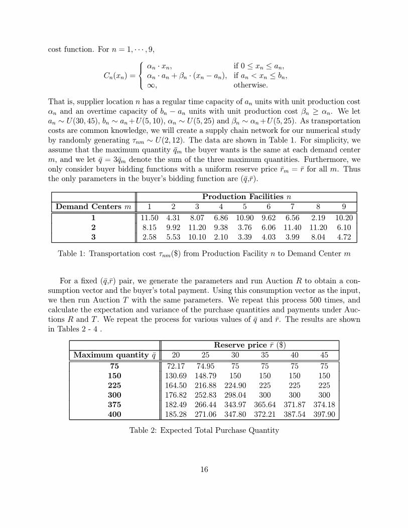
That is, supplier location n has a regular time capacity of an units with unit production costαn and an overtime capacity of bn − an units with unit production cost βn ≥ αn. We letan ∼ U(30, 45), bn ∼ an+U(5, 10), αn ∼ U(5, 25) and βn ∼ αn+U(5, 25). As transportationcosts are common knowledge, we will create a supply chain network for our numerical studyby randomly generating τnm ∼ U(2, 12). The data are shown in Table 1. For simplicity, weassume that the maximum quantity qm the buyer wants is the same at each demand centerm, and we let q = 3qm denote the sum of the three maximum quantities. Furthermore, weonly consider buyer bidding functions with a uniform reserve price rm = r for all m. Thusthe only parameters in the buyer’s bidding function are (q,r).

Production Facilities nDemand Centers m 1 2 3 4 5 6 7 8 9

1 11.50 4.31 8.07 6.86 10.90 9.62 6.56 2.19 10.202 8.15 9.92 11.20 9.38 3.76 6.06 11.40 11.20 6.103 2.58 5.53 10.10 2.10 3.39 4.03 3.99 8.04 4.72

Table 1: Transportation cost τnm($) from Production Facility n to Demand Center m

For a fixed (q,r) pair, we generate the parameters and run Auction R to obtain a con-sumption vector and the buyer’s total payment. Using this consumption vector as the input,we then run Auction T with the same parameters. We repeat this process 500 times, andcalculate the expectation and variance of the purchase quantities and payments under Auc-tions R and T . We repeat the process for various values of q and r. The results are shownin Tables 2 - 4 .

Reserve price r ($)Maximum quantity q 20 25 30 35 40 45

75 72.17 74.95 75 75 75 75150 130.69 148.79 150 150 150 150225 164.50 216.88 224.90 225 225 225300 176.82 252.83 298.04 300 300 300375 182.49 266.44 343.97 365.64 371.87 374.18400 185.28 271.06 347.80 372.21 387.54 397.90

Table 2: Expected Total Purchase Quantity

16

Reserve price r ($)Maximum quantity q 20 25 30 35 40 45

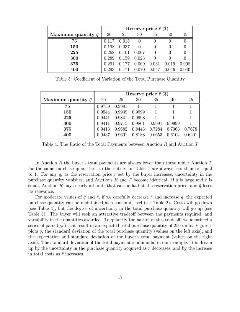
75 0.117 0.015 0 0 0 0150 0.198 0.037 0 0 0 0225 0.268 0.101 0.007 0 0 0300 0.289 0.159 0.023 0 0 0375 0.291 0.177 0.069 0.031 0.019 0.008400 0.293 0.171 0.070 0.047 0.046 0.040

Table 3: Coefficient of Variation of the Total Purchase Quantity

Reserve price r ($)Maximum quantity q 20 25 30 35 40 45

75 0.9759 0.9991 1 1 1 1150 0.9544 0.9939 0.9999 1 1 1225 0.9441 0.9841 0.9998 1 1 1300 0.9411 0.9715 0.9861 0.9991 0.9999 1375 0.9413 0.9682 0.8443 0.7284 0.7363 0.7678400 0.9437 0.9691 0.8188 0.6653 0.6104 0.6201

Table 4: The Ratio of the Total Payments between Auction R and Auction T

In Auction R the buyer’s total payments are always lower than those under Auction Tfor the same purchase quantities, so the entries in Table 4 are always less than or equalto 1. For any q, as the reservation price r set by the buyer increases, uncertainty in thepurchase quantity vanishes, and Auctions R and T become identical. If q is large and r issmall, Auction R buys nearly all units that can be had at the reservation price, and q losesits relevance.For moderate values of q and r, if we carefully decrease r and increase q, the expected

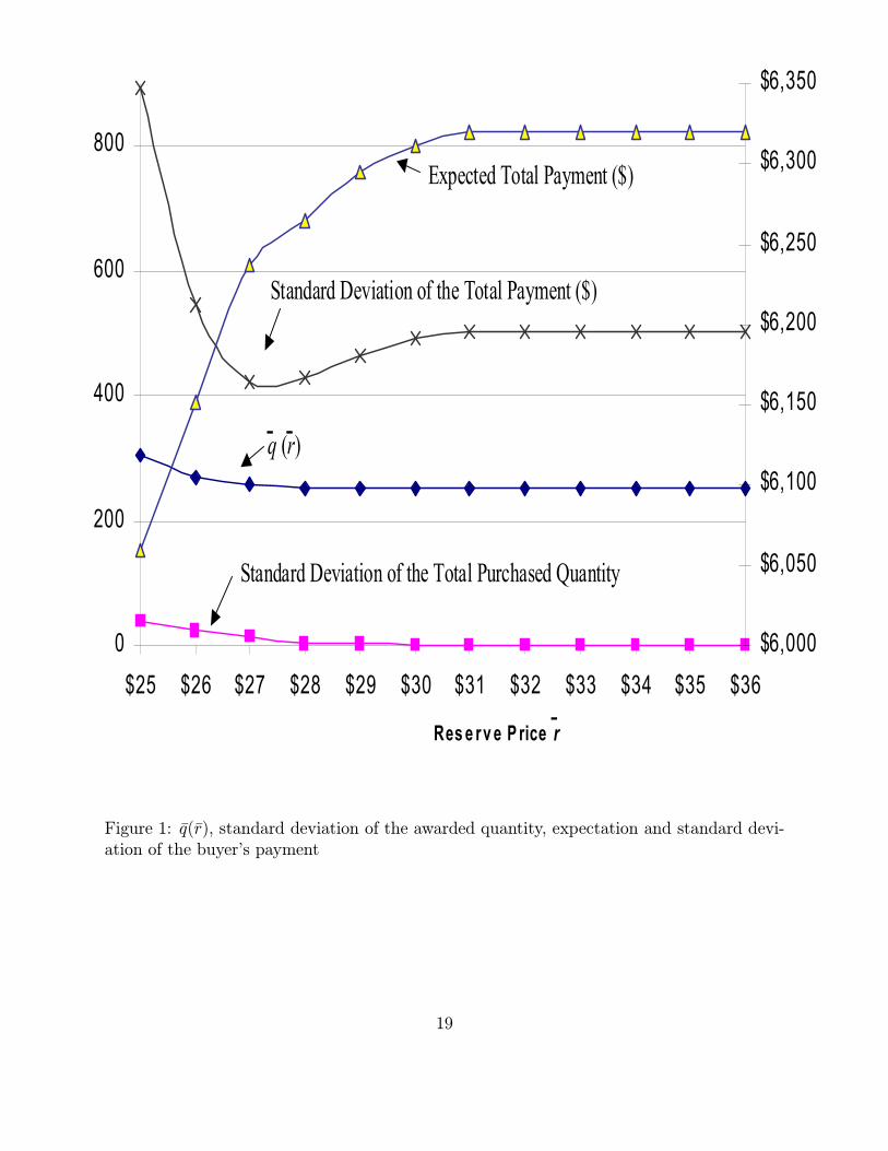
purchase quantity can be maintained at a constant level (see Table 2). Costs will go down(see Table 4), but the degree of uncertainty in the total purchase quantity will go up (seeTable 3). The buyer will seek an attractive tradeoff between the payments required, andvariability in the quantities awarded. To quantify the nature of this tradeoff, we identified aseries of pairs (q,r) that result in an expected total purchase quantity of 250 units. Figure 1plots q, the standard deviation of the total purchase quantity (values on the left axis), andthe expectation and standard deviation of the buyer’s total payment (values on the rightaxis). The standard deviation of the total payment is unimodal in our example. It is drivenup by the uncertainty in the purchase quantity acquired as r decreases, and by the increasein total costs as r increases.

17

The primary tradeoff is between the total payment, and variability in the purchase quan-tity. The buyer can control the size of his payments via a reservation price, but only byaccepting additional risks associated with the amount of material he acquires in the auction.

6 Auction S

Most literature in multi-unit auctions focuses on the cost of the product, ignoring other coststhat will be determined by the outcome of an auction. To examine the benefits of incorpo-rating transportation costs into auctions, we introduce Auction S, in which the auctioneerselects production quantities at supplier locations solely based on the suppliers’ bids andon demand, and the transportation decisions are made subsequently. For any consumptionvector q the buyer submits, the production quantities at different production facilities aredetermined by minimizing

PKk=1 Fk(xk) subject to constraints (4.2)-(4.4). Let πS(q) and x

S

be the optimal objective value and production vector, and π−kS (q) be the counter part ofπ−k(q). The buyer’s payment to supplier k in this auction, ψSk (q), is then given by

ψSk (q) = π−kS (q)− πS(q) + Fk(xSk ).

Under this payment structure, the suppliers will still submit their true cost functions andFk(xk) = Ck(xk) for all k. The transportation quantities y

Snm for all n and m are determined

by solving the following optimization problem

Min.NXn=1

MXm=1

τnmynm

s.t.NXn=1

ynm = qm, m = 1, . . . ,M,

MXm=1

ynm = xSn, n = 1, . . . ,N,

and the buyer’s total payment, κS(q), will be given by

κS(q) =KXk=1

ψSk (q) +NXn=1

MXm=1

τnmySnm.

It is obvious that Auction S leads to lower total production costs but higher supply chaincosts than Auction T . Our primary interests are the magnitude of the savings by runningAuction T and how the buyer’s payments differ in two auctions. We show that, underthe typical regular-overtime production cost structure, Auction T can lead to paymentsthat are large enough to distort buyer behavior. Intuitively, Auction T is most beneficialwhen the supplier locations and demand centers are geographically dispersed with distinct

18

0

200

400

600

800

$25 $26 $27 $28 $29 $30 $31 $32 $33 $34 $35 $36

Res e rv e P rice r

$6,000

$6,050

$6,100

$6,150

$6,200

$6,250

$6,300

$6,350

Standard Deviation of the Total Purchased Quantity

q (r)

Standard Deviation of the Total Payment ($)

Expected Total Payment ($)

-

- -

Figure 1: q(r), standard deviation of the awarded quantity, expectation and standard devi-ation of the buyer’s payment

19

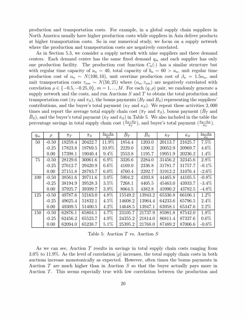
production and transportation costs. For example, in a global supply chain suppliers inNorth America usually have higher production costs while suppliers in Asia deliver productsat higher transportation costs. So in our numerical study, we focus on a supply networkwhere the production and transportation costs are negatively correlated.As in Section 5.3, we consider a supply network with nine suppliers and three demand

centers. Each demand center has the same fixed demand qm and each supplier has onlyone production facility. The production cost function Cn(·) has a similar structure butwith regular time capacity of an = 40, total capacity of bn = 60 > an, unit regular timeproduction cost of αn ∼ N(100, 10), unit overtime production cost of βn = 1.5αn, andunit transportation costs τnm ∼ N(50, 25) where (αn, τnm) are negatively correlated withcorrelation ρ ∈ {−0.5,−0.25, 0}, m = 1, ...,M . For each (q, ρ) pair, we randomly generate asupply network and the costs, and run Auctions S and T to obtain the total production andtransportation cost (πT and πS), the bonus payments (BT and BS) representing the suppliers’contributions, and the buyer’s total payment (κT and κS). We repeat these activities 2, 000times and report the average total supply chain cost (πT and πS), bonus payment (BT andBS), and the buyer’s total payment (κT and κS) in Table 5. We also included in the table thepercentage savings in total supply chain cost ( πS−πT

πT), and buyer’s total payment ( κS−κT

κT).

qm ρ πT πSπS−πTπT

BT BS κT κSκS−κTκT

50 -0.50 18259.4 20422.7 11.9% 1854.4 1203.0 20113.7 21625.7 7.5%-0.25 17823.8 19769.5 10.9% 2229.0 1200.2 20052.9 20969.7 4.6%0.00 17398.1 19040.4 9.4% 2553.8 1195.7 19951.9 20236.2 1.4%

75 -0.50 28129.6 30061.6 6.9% 3326.6 2284.0 31456.2 32345.6 2.8%-0.25 27612.7 29420.9 6.6% 4169.0 2336.8 31781.7 31757.7 -0.1%0.00 27151.8 28783.7 6.0% 4760.4 2292.7 31912.2 31076.4 -2.6%

100 -0.50 38561.6 39711.6 3.0% 5904.2 4393.8 44465.8 44105.5 -0.8%-0.25 38194.9 39528.3 3.5% 7268.1 4405.5 45463.0 43933.7 -3.4%0.00 37925.7 39399.7 3.9% 8064.5 4382.8 45990.2 43782.5 -4.8%

125 -0.50 49787.6 52163.0 4.8% 15549.2 13943.2 65336.8 66106.1 1.2%-0.25 49625.4 51832.1 4.5% 14608.2 13964.4 64233.6 65796.5 2.4%0.00 49309.5 51400.5 4.2% 14648.5 13947.1 63958.1 65347.6 2.2%

150 -0.50 62876.1 65804.1 4.7% 23105.7 21737.9 85981.8 87542.0 1.8%-0.25 62456.2 65523.7 4.9% 24355.2 21814.0 86811.4 87337.6 0.6%0.00 62094.0 65238.7 5.1% 25395.2 21768.0 87489.2 87006.6 -0.6%

Table 5: Auction T vs. Auction S

As we can see, Auction T results in savings in total supply chain costs ranging from3.0% to 11.9%. As the level of correlation |ρ| increases, the total supply chain costs in bothauctions increase monotonically as expected. However, often times the bonus payments inAuction T are much higher than in Auction S so that the buyer actually pays more inAuction T . This seems especially true with low correlation between the production and

20

transportation costs. As a result, the bonus portion of the total payments is usually higherin Auction T as shown in Table 6.Note that a bonus payment to a supplier in a Vickrey type auction measures the supplier’s

contribution to the system by comparing the total supply chain costs with and without thesupplier. The bonus payments can be higher in Auction T than Auction S for the followingtwo reasons.

• While the contribution of a supplier in Auction S is solely based on the productioncosts, the contribution of a supplier in Auction T takes both the production andtransportation costs into consideration. So a supplier has a higher impact on thetotal supply chain costs in Auction T than in Auction S and hence, receives a higherbonus payment. However, as correlation |ρ| increases, the difference of the total unitproduction and transportation costs among all suppliers becomes smaller and hencethe bonus payments in Auction T , in general, decrease. Often times, the differencebetween the supply chain costs outweighs the difference between the bonus payments,and Auction T leads to both lower total supply chain cost and total buyer’s payment.

• Auction S allocates production to the lowest cost suppliers while Auction T allocatesproduction to suppliers with the lowest production and transportation costs. Conse-quently, more overtime production is likely to be used in determining bonus paymentsin Auction T and the bonus payments can be significant, especially when the differencebetween regular time production costs and overtime production costs is big.

The behaviour of the buyer’s total payments, which are the sum of the total supply chaincost and the bonus payments, is more complex. When demand is low (qm = 50 in Table5), there is ample capacity in the system and the difference between the total supply chaincosts dominates the difference between the bonus payments. Hence, the buyer pays less inAuction T . As demand increases (qm = 75, 100), more overtime capacity is involved indetermining the bonus payments in Auction T and the buyer pays more in Auction T . Asdemand continues to increase (qm = 125), a small amount of overtime production is neededto meet the demand in both auctions. The impact of the overtime costs is similar in bothauctions and, in general, the buyer pays less in Auction T . However, at higher demand level(qm = 150), the transportation costs cause the bonus payments to be much higher in AuctionT than Auction S, especially when |ρ| is small, and the buyer pays more in Auction T .In most manufacturing systems, per-unit costs are relatively flat when the regular-time

capacity of the manufacturing system is not exceeded, while the marginal per-unit productioncosts grow rapidly when overtime or other measures are required to increase capacity in theshort term. As we can see, such cost structure can lead to higher total payments in AuctionT , making Auction S more preferable to the buyer, although it is less efficient for the overallsupply chain. One might conclude that this counter-intuitive situation is caused by ourselection of the VCG payment mechanism. However under mild assumptions, the RevenueEquivalence Theorem (Engelbrecht-Wiggans 1988) indicates that any auction mechanismthat results in an efficient solution will reward the suppliers with the same expected revenue.

21

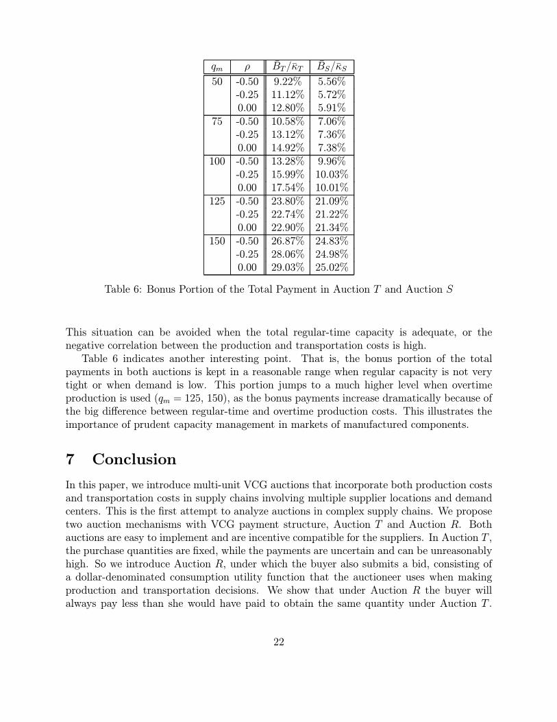
qm ρ BT/κT BS/κS

50 -0.50 9.22% 5.56%-0.25 11.12% 5.72%0.00 12.80% 5.91%

75 -0.50 10.58% 7.06%-0.25 13.12% 7.36%0.00 14.92% 7.38%

100 -0.50 13.28% 9.96%-0.25 15.99% 10.03%0.00 17.54% 10.01%

125 -0.50 23.80% 21.09%-0.25 22.74% 21.22%0.00 22.90% 21.34%

150 -0.50 26.87% 24.83%-0.25 28.06% 24.98%0.00 29.03% 25.02%

Table 6: Bonus Portion of the Total Payment in Auction T and Auction S

This situation can be avoided when the total regular-time capacity is adequate, or thenegative correlation between the production and transportation costs is high.Table 6 indicates another interesting point. That is, the bonus portion of the total

payments in both auctions is kept in a reasonable range when regular capacity is not verytight or when demand is low. This portion jumps to a much higher level when overtimeproduction is used (qm = 125, 150), as the bonus payments increase dramatically because ofthe big difference between regular-time and overtime production costs. This illustrates theimportance of prudent capacity management in markets of manufactured components.

7 Conclusion

In this paper, we introduce multi-unit VCG auctions that incorporate both production costsand transportation costs in supply chains involving multiple supplier locations and demandcenters. This is the first attempt to analyze auctions in complex supply chains. We proposetwo auction mechanisms with VCG payment structure, Auction T and Auction R. Bothauctions are easy to implement and are incentive compatible for the suppliers. In Auction T ,the purchase quantities are fixed, while the payments are uncertain and can be unreasonablyhigh. So we introduce Auction R, under which the buyer also submits a bid, consisting ofa dollar-denominated consumption utility function that the auctioneer uses when makingproduction and transportation decisions. We show that under Auction R the buyer willalways pay less than she would have paid to obtain the same quantity under Auction T .

22

Consequently, if the buyer can anticipate the bids of the suppliers (complete information),she will always prefer Auction R. We derive the buyer’s optimal bidding function thatmaximizes her net utility under complete information. However, if the buyer lacks completeinformation, both the awarded quantities and the buyer’s payments are random variables inAuction R. This adds a new element of risk that needs to be traded off against the costsavings that the buyer realizes with Auction R. In practice a computational approach canbe used to make this tradeoff.To illustrate the importance of incorporating transportation costs into auctions, we con-

sider Auction S, under which the auctioneer awards quantities solely based on the suppliers’bids and the demand, and the transportation decisions are made subsequently. AlthoughAuction S is incentive compatible, numerical examples show that considerable supply chaincost savings can be achieved by running Auction T . However, the buyer may favor AuctionS due to lower total payments under certain circumstances. This is because, in Auction T ,a supplier’s contribution is measured not only by its production costs, but also the trans-portation costs. When the system-wide regular capacity is tight, overtime production andtransportation costs together drive the payments up dramatically. The possible higher pay-ments in Auction T can induce the buyer to favor the inefficient solution, Auction S. Thisillustrates the vital importance of prudent capacity management in markets of manufacturedcomponents.This work can be easily extended to VCG auctions with one supplier and multiple buyers.

Other costs that might arise when parts are purchased in supply chain settings can also beincluded, including fixed costs and other economies of scale. However with some of theseextensions the required computational effort will increase. Future work also includes auctionsin supply chains with multiple suppliers and buyers.

8 Appendix

Proof of Property 2: The first two results follow directly from Theorem 28.3 of Rockafellar(1970). We now prove that v ∈ ∂π(q). The proof for v ∈ ∂π−k(q − zTk ) is similar and isomitted here.Let (xT (q0),yT (q0)) represent an optimal solution for q0 ∈ Q. Then,

π(q0)− π(q) =KXk=1

[Ck(xTk (q

0))− Ck(xTk )] +NXn=1

MXm=1

τnm[yTnm(q

0)− yTnm]

≥KXk=1

uk · [xTk (q0)− xTk ] +NXn=1

MXm=1

τnm[yTnm(q

0)− yTnm]

=NXn=1

unMXm=1

[yTnm(q0)− yTnm] +

NXn=1

MXm=1

τnm[yTnm(q

0)− yTnm]

=NXn=1

MXm=1

(un + τnm)[yTnm(q

0)− yTnm]

23

=X

n,m:yTnm(q)>0

vm[yTnm(q

0)− yTnm] +X

n,m:yTnm=0

(un + τnm)yTnm(q

0)

≥ Xn,m:yTnm>0

vm[yTnm(q

0)− yTnm(q)] +X

n,m:yTnm=0

vmyTnm(q

0)

=MXm=1

vmNXn=1

[yTnm(q0)− yTnm] =

MXm=1

vm(q0m − qm) = v · (q0 − q).

The inequalities follow from the first two results and the nonnegativity of yTnm(q0).

2

Proof of Lemma 3: Consider the equivalent T auction with fixed demand qmax =qR + xRB resulting from a concave function W (·). Recall that the equivalent T auction hasthe minimum cost Π(W ) = π(qR) + FB(x

RB). By Property 2, we have the first two results.

To show that r ∈ ∂W (qR), it suffices to prove that r ∈ ∂FB(xRB) by the definition of

FB(·). Consider any vector x0B ∈ RM and, without loss of generality, 0 ≤ x0B ≤ qmax.FB(x

0B)− FB(xRB) ≥ uB · (x0B − xRB) =

Xm:qRm>0

uBm(x0Bm − xRBm) +

Xm:qRm=0

uBm(x0Bm − xRBm).

Note that qRm = 0 implies that xRBm = qmaxm and x0Bm − xRBm ≤ 0. Since 0 ≤ uBm ≤ rm ifqRm = 0, and uBm = rm if q

Rm > 0, we have

FB(x0B)− FB(xRB) ≥

Xm:qRm>0

rm(x0Bm − xRBm) +

Xm:qRm=0

rm(x0Bm − xRBm) = r · (x0B − xRB).

The proof of Property 2 establishes the rest of the lemma.

2

Proof of Lemma 4: For any r ∈ γ(W,qR), let (xR,yR) be an solution associated withit. Rewrite κR(W ) as

κR(W ) =KXk=1

[π−k(qR−k)−W (qR−k)]−K[π(qR)−W (qR)] + π(qR).

Recall that the production and transportation quantities resulting from the T auction forgiven qR are the same as those from the R auction with qR as the output. Also, zRkm =Pn∈Nk yRnm, the total quantity shipped to demand center m by supplier k. Hence, Property

3 leads to

π(qR) = π−k(qR − zRk ) + Fk(xRk ) +Xn∈Nk

MXm=1

τnmyRnm,

(1−K)π(qR) = π(qR)−KXk=1

π(qR) = −KXk=1

π−k(qR − zRk ),

24

and

κR(W ) =KXk=1

[π−k(qR−k)− π−k(qR − zRk ) +W (qR)−W (qR−k)].

For any r ∈ γ(W,qR), r ∈ ∂π−k(qR − zRk ) and r ∈ ∂W (qR) by Lemma 3. As π−k(·) isconvex and W (·) is concave,

π−k(qR−k)− π−k(qR − zRk ) ≥ r · [qR−k − (qR − zRk )]W (qR)−W (qR−k) ≥ r · (qR − qR−k).

Hence,

κR(W ) ≥KXk=1

r · [qR−k − (qR − zRk ) + (qR − qR−k)] =KXk=1

r · zRk = r · qR.

2

Proof of Lemma 5: If the buyer submits W (q), the auctioneer will minimize {π(q)−W (q)} to obtain the consumption vector.We know that, for r ∈ Γ(q), r ∈ ∂π(q). By the way W (·) is constructed, r ∈ ∂W (q).

So 0 ∈ ∂π(q) − ∂W (q). By Theorem 23.8 of Rockafellar (1970), 0 ∈ ∂[π(q) − W (q)]. Asπ(q) − W (q) is a convex program, q minimizes {π(q) − W (q)}. Let (x, y) be an solutionassociated with r and zk =

Pn∈Nk

ynm. Following the same arguments, q − zk minimizes{π−k(q)− W (q)} and, for any qR−k that minimizes {π−k(q)− W (q)},

π−k(qR−k)− W (qR−k) = π−k(q− zk)− W (q− zk). (8.9)

Since Ck(·) is strictly increasing for all k, π(q) is strictly increasing for any q ∈ Q. Ifthere exist multiple solutions to min{π(q) − W (q)}, the auctioneer will always choose anoptimal consumption vector with the largest total purchase quantity as we assumed earlier.We claim that qR = q. Suppose there exists an optimal solution with qm > qm for some m.Then W (q ∧ q) = W (q), but π(q ∧ q) < π(q). Thus q cannot be optimal.The buyer’s total payment is given by

κR(W ) =KXk=1

[π−k(qR−k)− W (qR−k)]−KXk=1

[π(q)− W (q)] + π(q)

=KXk=1

[W (q)− W (qR−k)] +KXk=1

[π−k(qR−k)− π(q)] + π(q)

=KXk=1

[W (q)− W (q− zk)] +KXk=1

[π−k(q− zk)− π(q)] + π(q).

25

The last equality follows from Equation (8.9). By Property 3,

π(q) = π−k(q− zk) + Ck(xk) +Xn∈Nk

MXm=1

τnmynm.

Summing over k, we have

π(q) = −KXk=1

[π−k(q− zk)− π(q)],

and

κR(W ) =KXk=1

[W (q)− W (q− zk)] =MXm=1

Xn∈Nk

rm · ynm = r · q.

That is, the buyer pays a uniform price rm, for all the units shipped to demand center m.

2

Proof of Theorem 6: If the buyer submits W ∗(q), by Lemma 5, the resulting con-sumption vector is q∗R = q∗, the buyer’s total payment is κR(W ∗) = r∗ · q∗, and the buyerpays a uniform price r∗m for all units shipped to demand center m. For any W (q) resultingin qR as the output of Auction R, by Lemma 4,

U(qR)− κR(W ) ≤ U(qR)− r · qR

for all r ∈ γ(W,qR) ⊆ Γ(qR). For any r ∈ Γ(qR),U(qR)− r · qR ≤ U(qR)− r∗(qR) · qR ≤ U(q∗)− r∗ · q∗.

So

U(qR)− κR(W ) ≤ U(q∗)− r∗ · q∗.That is, in Auction R, the buyer’s utility is maximized by submitting W ∗(q).

2

Proof of Lemma 7: For any given r ∈ Γ(q), r ∈ γ(W,qR) for some W satisfyingAssumption 3 with qR = q. The associated (xR,yR,u,uB) satisfies Lemma 3 and hence,(xR,yR,u, r) satisfies Property 2. Therefore, r ∈ V (q).For any given v ∈ V (q), there exists (xT ,yT ,u) satisfying Property 2. Hence, v ∈ ∂π(q)

and v ∈ ∂π−k(q − zTk ). We can construct W (q) as defined in Lemma 5 with parameter vinstead of a r from set Γ(q). By similar arguments in the proof of Lemma 5, W (·) results inqR = q and hence, v ∈ γ(W ,q). Therefore, v ∈ Γ(q) and Γ(q) = V (q) for any q ∈ Q.

2

26

9 References

Ausubel, L. and P. Cramton, 1998, “Demand Reduction and Inefficiency in Multi-UnitAuctions”, Department of Economics, University of Maryland, Working Paper No.96-07.

Beil, D. R. and L. Wein, 2001, “An Inverse-Optimization-Based Auction Mechanism toSupport a Multi-Attribute RFQ Process, Working paper, Sloan School of Management,MIT.

Chopra, S. and J. Van Mieghem, 2000, “Which e-business is right for your supply chain?”,Supply Chain Management Review, 4(3), 32-40.

Clarke, E. H., 1971, “Multipart Pricing of Public Goods”, Public Choice, 11, 17-33.

Engelbrecht-Wiggans, R., 1988, “Revenue Equivalence in Multi-object Auctions”, Eco-nomic Letters, 26, 15-19.

Eso, M., 2001, “An iterative onling auction for airline seats.”, Technical report, IBM T. J.Watson Research Center.

Ethier, R., R. Zimmerman, T. Mount, W. Schulze and R. Thomas, 1999, “A UniformPrice Auction with Locational Price Adjustments for Competitive Electricity Markets”,Electrical Power and Energy Systems, 21, 103-110.

Groves, T., 1973, “Incentive in Teams”, Econometrica, 41, 617-631.

Holmberg, K. and H. Tuy, 1999, “A production-transportation problem with stochasticdemand and concave production costs”, Mathematical Programming, 85, 157-179.

Jin, M. and S. D. Wu, 2001, “Supplier Coalitions in eCommerce Auctions: Validity Re-quirements and Profit Distribution”, Working paper, Department of Industrial andSystems Engineering, Lehigh University.

Klemperer, P., 1999, “Auction theory: A guide to the literature.”, Journal of EconomicSurveys, 13(3), 227-186.

Keskinocak, P. and S. Tayur, 2001, “Quantitative Analysis for Internet-Enabled SupplyChains”, Interfaces, 31(2), 70-89.

Lucking-Riley, D., 2000, “Auctions on the Internet: What’s Being Auctioned, and How?”,Journal of Industrial Economics, 48(3), 227-252.

McAfee, R. P. and J. McMillan, 1987, “Auction and bidding”, Journal of Economic Liter-ature, 25(2), 699-738.

27

Milgrom, P. and R. Weber, 1982, “A theory of auctions and competitive bidding. ”, Econo-metrica, 50(5), 1089-1122.

Nisan, N. and A. Ronen, 2001, “Algorithmic Mechanism Design”, Games and EconomicBehavior, 35(1/2), 166-196.

Pinker, E., A. Seidmann and Y. Vakrat, 2001, “Using Transaction Data for the Designof Sequential, Multi-unit, Online Auctions”, Working Paper, W. E. Simon GraduateSchool of Business Administration, University of Rochester.

Rockafellar, R. T., 1970, Convex Analysis, Princeton University Press, Princeton, NewJersey.

Rothkopf, M. H., 1969, “A Model of Rational Competitive Bidding”, Management Science,15(7), 362-373.

Rothkopf, M. H. and R. M. Harstad, 1994, “Modeling Competitive Bidding: A CriticalEssay”, Management Science, 40(3), 364-384.

Rothkopf, M. H., A. Pekec, and R. H. Harstad, 1998, “Computationally manageable com-binatorial auctions”, Management Science, 44(8), 1131-1147.

Rothkopf, M. H., T. J. Teisberg, and E. P. Kahn, 1990, “Why are Vickrey auctions rare?”Journal of Political Economy, 98(1),94-109.

Sharp, J. F., J. C. Snyder and J. H. Greene, 1970, “A Decomposition Algorithm for Solv-ing the Multifacility Production-Transportation Problem with Non-linear ProductionCosts”, Econometrica, 38(3), 490-506.

Sullivan, L. and R. Lamb, “Rift Grows Over Pricing in Supply Chain”, Electronics BusinessNetwork, November 19, 2001, http://www.ebnews.com.

Vickrey, W., 1961, “Counterspeculation, Auctions, and Competitive Sealed Tenders”, Jour-nal of Finance, 16, 8-37.

Vulcano, G., G. van Ryzin and C. Maglaras, 2001, “Optimal Dynamic Auctions for RevenueManagement”, Working Paper, Graduate School of Business, Columbia University.

28