Embed Size (px)
Citation preview

SS 2018/19
Efficient Algorithmsand Data Structures II
Harald Räcke
Fakultät für InformatikTU München
http://www14.in.tum.de/lehre/2018SS/ea/
Summer Term 2018/19
6. Jul. 2018
Harald Räcke 1/554

Part I
Organizational Matters
6. Jul. 2018
Harald Räcke 2/554

Part I
Organizational Matters
ñ Modul: IN2004
ñ Name: “Efficient Algorithms and Data Structures II”
“Effiziente Algorithmen und Datenstrukturen II”
ñ ECTS: 8 Credit points
ñ Lectures:ñ 4 SWS
Wed 12:15–13:45 (Room 00.13.009A)Fri 10:15–11:45 (MS HS3)
ñ Webpage: http://www14.in.tum.de/lehre/2018SS/ea/
6. Jul. 2018
Harald Räcke 3/554

The Lecturer
ñ Harald Räcke
ñ Email: [email protected]
ñ Room: 03.09.044
ñ Office hours: (per appointment)
6. Jul. 2018
Harald Räcke 4/554

Tutorials
ñ Tutor:ñ Richard Stotzñ [email protected]ñ Room: 03.09.057ñ per appointment
ñ Room: 03.11.018
ñ Time: Mon 14:00–15:30
6. Jul. 2018
Harald Räcke 5/554

Assessment
ñ In order to pass the module you need to pass an exam.
ñ Exam:ñ 2.5 hoursñ Date will be announced shortly.ñ There are no resources allowed, apart from a hand-written
piece of paper (A4).ñ Answers should be given in English, but German is also
accepted.
6. Jul. 2018
Harald Räcke 6/554

Assessment
ñ Assignment Sheets:ñ An assignment sheet is usually made available on Monday
on the module webpage.ñ Solutions have to be handed in in the following week before
the tutorial on Monday.ñ You can hand in your solutions by putting them in the right
folder in front of room 03.09.020 or in person in thetutorial.
ñ Solutions have to be given in English.ñ Solutions will be discussed in the subsequent tutorial.ñ The first one will be out on Monday, 16 April.
6. Jul. 2018
Harald Räcke 7/554

1 Contents
Part 1: Linear Programming
Part 2: Approximation Algorithms
1 Contents 6. Jul. 2018
Harald Räcke 8/554

2 Literatur
V. Chvatal:
Linear Programming,
Freeman, 1983
R. Seidel:
Skript Optimierung, 1996
D. Bertsimas and J.N. Tsitsiklis:
Introduction to Linear Optimization,
Athena Scientific, 1997
Vijay V. Vazirani:
Approximation Algorithms,
Springer 2001
2 Literatur 6. Jul. 2018
Harald Räcke 9/554

David P. Williamson and David B. Shmoys:
The Design of Approximation Algorithms,
Cambridge University Press 2011
G. Ausiello, P. Crescenzi, G. Gambosi, V. Kann, A.
Marchetti-Spaccamela, and M. Protasi:
Complexity and Approximation,
Springer, 1999
2 Literatur 6. Jul. 2018
Harald Räcke 10/554

Part II
Linear Programming
6. Jul. 2018
Harald Räcke 11/554

Brewery Problem
Brewery brews ale and beer.
ñ Production limited by supply of corn, hops and barley malt
ñ Recipes for ale and beer require different amounts of
resources
Corn
(kg)
Hops
(kg)
Malt
(kg)Profit
(€)
ale (barrel) 5 4 35 13beer (barrel) 15 4 20 23
supply 480 160 1190
3 Introduction to Linear Programming 6. Jul. 2018
Harald Räcke 12/554

Brewery Problem
Corn
(kg)
Hops
(kg)
Malt
(kg)Profit
(€)
ale (barrel) 5 4 35 13beer (barrel) 15 4 20 23
supply 480 160 1190
How can brewer maximize profits?
ñ only brew ale: 34 barrels of ale =⇒ 442 €
ñ only brew beer: 32 barrels of beer =⇒ 736 €
ñ 7.5 barrels ale, 29.5 barrels beer =⇒ 776 €
ñ 12 barrels ale, 28 barrels beer =⇒ 800 €
3 Introduction to Linear Programming 6. Jul. 2018
Harald Räcke 13/554

Brewery Problem
Linear Program
ñ Introduce variables a and b that define how much ale and
beer to produce.
ñ Choose the variables in such a way that the objective
function (profit) is maximized.
ñ Make sure that no constraints (due to limited supply) are
violated.
max 13a + 23b
s.t. 5a + 15b ≤ 480
4a + 4b ≤ 160
35a + 20b ≤ 1190
a,b ≥ 0
3 Introduction to Linear Programming 6. Jul. 2018
Harald Räcke 14/554

Standard Form LPs
LP in standard form:
ñ input: numbers aij, cj, biñ output: numbers xjñ n = #decision variables, m = #constraints
ñ maximize linear objective function subject to linear
(in)equalities
maxn∑
j=1
cjxj
s.t.n∑
j=1
aijxj = bi 1 ≤ i ≤m
xj ≥ 0 1 ≤ j ≤ n
max cTxs.t. Ax = b
x ≥ 0
3 Introduction to Linear Programming 6. Jul. 2018
Harald Räcke 15/554

Standard Form LPs
Original LPmax 13a + 23b
s.t. 5a + 15b ≤ 480
4a + 4b ≤ 160
35a + 20b ≤ 1190
a,b ≥ 0
Standard Form
Add a slack variable to every constraint.
max 13a + 23b
s.t. 5a + 15b + sc = 480
4a + 4b + sh = 160
35a + 20b + sm = 1190
a , b , sc , sh , sm ≥ 0
3 Introduction to Linear Programming 6. Jul. 2018
Harald Räcke 16/554

Standard Form LPs
There are different standard forms:
standard form
max cTxs.t. Ax = b
x ≥ 0
min cTxs.t. Ax = b
x ≥ 0
standardmaximization form
max cTxs.t. Ax ≤ b
x ≥ 0
standardminimization form
min cTxs.t. Ax ≥ b
x ≥ 0
3 Introduction to Linear Programming 6. Jul. 2018
Harald Räcke 17/554

Standard Form LPs
It is easy to transform variants of LPs into (any) standard form:
ñ less or equal to equality:
a− 3b + 5c ≤ 12 =⇒ a− 3b + 5c + s = 12
s ≥ 0
ñ greater or equal to equality:
a− 3b + 5c ≥ 12 =⇒ a− 3b + 5c − s = 12
s ≥ 0
ñ min to max:
mina− 3b + 5c =⇒ max−a+ 3b − 5c
3 Introduction to Linear Programming 6. Jul. 2018
Harald Räcke 18/554

Standard Form LPsIt is easy to transform variants of LPs into (any) standard form:
ñ equality to less or equal:
a− 3b + 5c = 12 =⇒ a− 3b + 5c ≤ 12
−a+ 3b − 5c ≤ −12
ñ equality to greater or equal:
a− 3b + 5c = 12 =⇒ a− 3b + 5c ≥ 12
−a+ 3b − 5c ≥ −12
ñ unrestricted to nonnegative:
x unrestricted =⇒ x = x+ − x−, x+ ≥ 0, x− ≥ 0
3 Introduction to Linear Programming 6. Jul. 2018
Harald Räcke 19/554

Standard Form LPs
Observations:
ñ a linear program does not contain x2, cos(x), etc.
ñ transformations between standard forms can be done
efficiently and only change the size of the LP by a small
constant factor
ñ for the standard minimization or maximization LPs we could
include the nonnegativity constraints into the set of
ordinary constraints; this is of course not possible for the
standard form
3 Introduction to Linear Programming 6. Jul. 2018
Harald Räcke 20/554

Fundamental Questions
Definition 1 (Linear Programming Problem (LP))
Let A ∈ Qm×n, b ∈ Qm, c ∈ Qn, α ∈ Q. Does there exist
x ∈ Qn s.t. Ax = b, x ≥ 0, cTx ≥ α?
Questions:
ñ Is LP in NP?
ñ Is LP in co-NP?
ñ Is LP in P?
Input size:
ñ n number of variables, m constraints, L number of bits to
encode the input
3 Introduction to Linear Programming 6. Jul. 2018
Harald Räcke 21/554
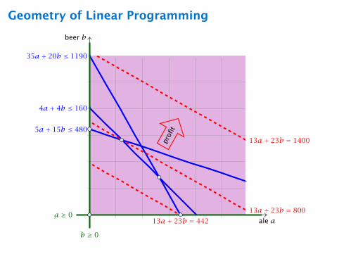
Geometry of Linear Programming
ale a
beer b
4a+ 4b ≤ 160
5a+ 15b ≤ 480
35a+ 20b ≤ 1190
13a+ 23b = 442
13a+ 23b = 800
13a+ 23b = 1400
a ≥ 0
b ≥ 0
profi
t

Geometry of Linear Programming
ale a
beer b
profi
t
Regardless of the objective function an
optimum solution occurs at a vertex
(Ecke).

Definitions
Let for a Linear Program in standard form
P = x | Ax = b,x ≥ 0.ñ P is called the feasible region (Lösungsraum) of the LP.
ñ A point x ∈ P is called a feasible point (gültige Lösung).
ñ If P ≠ then the LP is called feasible (erfüllbar). Otherwise,
it is called infeasible (unerfüllbar).
ñ An LP is bounded (beschränkt) if it is feasible andñ cTx <∞ for all x ∈ P (for maximization problems)ñ cTx > −∞ for all x ∈ P (for minimization problems)
3 Introduction to Linear Programming 6. Jul. 2018
Harald Räcke 24/554

Definition 2
Given vectors/points x1, . . . , xk ∈ Rn,∑λixi is called
ñ linear combination if λi ∈ R.
ñ affine combination if λi ∈ R and∑i λi = 1.
ñ convex combination if λi ∈ R and∑i λi = 1 and λi ≥ 0.
ñ conic combination if λi ∈ R and λi ≥ 0.
Note that a combination involves only finitely many vectors.
3 Introduction to Linear Programming 6. Jul. 2018
Harald Räcke 25/554

Definition 3
A set X ⊆ Rn is called
ñ a linear subspace if it is closed under linear combinations.
ñ an affine subspace if it is closed under affine combinations.
ñ convex if it is closed under convex combinations.
ñ a convex cone if it is closed under conic combinations.
Note that an affine subspace is not a vector space
3 Introduction to Linear Programming 6. Jul. 2018
Harald Räcke 26/554

Definition 4
Given a set X ⊆ Rn.
ñ span(X) is the set of all linear combinations of X(linear hull, span)
ñ aff(X) is the set of all affine combinations of X(affine hull)
ñ conv(X) is the set of all convex combinations of X(convex hull)
ñ cone(X) is the set of all conic combinations of X(conic hull)
3 Introduction to Linear Programming 6. Jul. 2018
Harald Räcke 27/554

Definition 5
A function f : Rn → R is convex if for x,y ∈ Rn and λ ∈ [0,1]we have
f(λx + (1− λ)y) ≤ λf(x)+ (1− λ)f(y)
Lemma 6
If P ⊆ Rn, and f : Rn → R convex then also
Q = x ∈ P | f(x) ≤ t
3 Introduction to Linear Programming 6. Jul. 2018
Harald Räcke 28/554

Dimensions
Definition 7
The dimension dim(A) of an affine subspace A ⊆ Rn is the
dimension of the vector space x − a | x ∈ A, where a ∈ A.
Definition 8
The dimension dim(X) of a convex set X ⊆ Rn is the dimension
of its affine hull aff(X).
3 Introduction to Linear Programming 6. Jul. 2018
Harald Räcke 29/554

Definition 9
A set H ⊆ Rn is a hyperplane if H = x | aTx = b, for a ≠ 0.
Definition 10
A set H′ ⊆ Rn is a (closed) halfspace if H = x | aTx ≤ b, for
a ≠ 0.
3 Introduction to Linear Programming 6. Jul. 2018
Harald Räcke 30/554

Definitions
Definition 11
A polytop is a set P ⊆ Rn that is the convex hull of a finite set of
points, i.e., P = conv(X) where |X| = c.
3 Introduction to Linear Programming 6. Jul. 2018
Harald Räcke 31/554
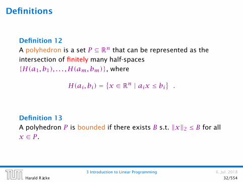
Definitions
Definition 12
A polyhedron is a set P ⊆ Rn that can be represented as the
intersection of finitely many half-spaces
H(a1, b1), . . . ,H(am, bm), where
H(ai, bi) =x ∈ Rn | aix ≤ bi
.
Definition 13
A polyhedron P is bounded if there exists B s.t. ‖x‖2 ≤ B for all
x ∈ P .
3 Introduction to Linear Programming 6. Jul. 2018
Harald Räcke 32/554

Definitions
Theorem 14
P is a bounded polyhedron iff P is a polytop.
3 Introduction to Linear Programming 6. Jul. 2018
Harald Räcke 33/554

Definition 15
Let P ⊆ Rn, a ∈ Rn and b ∈ R. The hyperplane
H(a,b) = x ∈ Rn | aTx = b
is a supporting hyperplane of P if maxaTx | x ∈ P = b.
Definition 16
Let P ⊆ Rn. F is a face of P if F = P or F = P ∩H for some
supporting hyperplane H.
Definition 17
Let P ⊆ Rn.
ñ a face v is a vertex of P if v is a face of P .
ñ a face e is an edge of P if e is a face and dim(e) = 1.
ñ a face F is a facet of P if F is a face and
dim(F) = dim(P)− 1.
3 Introduction to Linear Programming 6. Jul. 2018
Harald Räcke 34/554

Equivalent definition for vertex:
Definition 18
Given polyhedron P . A point x ∈ P is a vertex if ∃c ∈ Rn such
that cTy < cTx, for all y ∈ P , y ≠ x.
Definition 19
Given polyhedron P . A point x ∈ P is an extreme point if
a,b ≠ x, a,b ∈ P , with λa+ (1− λ)b = x for λ ∈ [0,1].
Lemma 20
A vertex is also an extreme point.
3 Introduction to Linear Programming 6. Jul. 2018
Harald Räcke 35/554

Observation
The feasible region of an LP is a Polyhedron.
3 Introduction to Linear Programming 6. Jul. 2018
Harald Räcke 36/554

Convex Sets
Theorem 21
If there exists an optimal solution to an LP (in standard form)
then there exists an optimum solution that is an extreme point.
Proof
ñ suppose x is optimal solution that is not extreme point
ñ there exists direction d ≠ 0 such that x ± d ∈ Pñ Ad = 0 because A(x ± d) = bñ Wlog. assume cTd ≥ 0 (by taking either d or −d)
ñ Consider x + λd, λ > 0
3 Introduction to Linear Programming 6. Jul. 2018
Harald Räcke 37/554

Convex Sets
Case 1. [∃j s.t. dj < 0]
ñ increase λ to λ′ until first component of x + λd hits 0
ñ x + λ′d is feasible. Since A(x + λ′d) = b and x + λ′d ≥ 0
ñ x + λ′d has one more zero-component (dk = 0 for xk = 0 as
x ± d ∈ P )
ñ cTx′ = cT (x + λ′d) = cTx + λ′cTd ≥ cTx
Case 2. [dj ≥ 0 for all j and cTd > 0]
ñ x + λd is feasible for all λ ≥ 0 since A(x + λd) = b and
x + λd ≥ x ≥ 0
ñ as λ→∞, cT (x + λd)→∞ as cTd > 0
3 Introduction to Linear Programming 6. Jul. 2018
Harald Räcke 38/554

Algebraic View
ale a
beer b
An extreme point in Rd is uniquely de-
fined by d linearly independent equa-
tions.
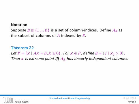
Notation
Suppose B ⊆ 1 . . . n is a set of column-indices. Define AB as
the subset of columns of A indexed by B.
Theorem 22
Let P = x | Ax = b,x ≥ 0. For x ∈ P , define B = j | xj > 0.Then x is extreme point iff AB has linearly independent columns.
3 Introduction to Linear Programming 6. Jul. 2018
Harald Räcke 40/554

Theorem 22
Let P = x | Ax = b,x ≥ 0. For x ∈ P , define B = j | xj > 0.Then x is extreme point iff AB has linearly independent columns.
Proof (⇐)
ñ assume x is not extreme point
ñ there exists direction d s.t. x ± d ∈ Pñ Ad = 0 because A(x ± d) = bñ define B′ = j | dj ≠ 0ñ AB′ has linearly dependent columns as Ad = 0
ñ dj = 0 for all j with xj = 0 as x ± d ≥ 0
ñ Hence, B′ ⊆ B, AB′ is sub-matrix of AB
3 Introduction to Linear Programming 6. Jul. 2018
Harald Räcke 41/554

Theorem 22
Let P = x | Ax = b,x ≥ 0. For x ∈ P , define B = j | xj > 0.Then x is extreme point iff AB has linearly independent columns.
Proof (⇒)
ñ assume AB has linearly dependent columns
ñ there exists d ≠ 0 such that ABd = 0
ñ extend d to Rn by adding 0-components
ñ now, Ad = 0 and dj = 0 whenever xj = 0
ñ for sufficiently small λ we have x ± λd ∈ Pñ hence, x is not extreme point
3 Introduction to Linear Programming 6. Jul. 2018
Harald Räcke 42/554

Theorem 23
Let P = x | Ax = b,x ≥ 0. For x ∈ P , define B = j | xj > 0.If AB has linearly independent columns then x is a vertex of P .
ñ define cj =
0 j ∈ B−1 j ∉ B
ñ then cTx = 0 and cTy ≤ 0 for y ∈ Pñ assume cTy = 0; then yj = 0 for all j ∉ Bñ b = Ay = AByB = Ax = ABxB gives that AB(xB −yB) = 0;
ñ this means that xB = yB since AB has linearly independent
columns
ñ we get y = xñ hence, x is a vertex of P
3 Introduction to Linear Programming 6. Jul. 2018
Harald Räcke 43/554

Observation
For an LP we can assume wlog. that the matrix A has full
row-rank. This means rank(A) =m.
ñ assume that rank(A) < mñ assume wlog. that the first row A1 lies in the span of the
other rows A2, . . . , Am; this means
A1 =∑m
i=2λi ·Ai, for suitable λi
C1 if now b1 =∑mi=2 λi · bi then for all x with Aix = bi we also
have A1x = b1; hence the first constraint is superfluous
C2 if b1 ≠∑mi=2 λi · bi then the LP is infeasible, since for all x
that fulfill constraints A2, . . . , Am we have
A1x =∑m
i=2λi ·Aix =
∑m
i=2λi · bi ≠ b1

From now on we will always assume that the
constraint matrix of a standard form LP has full
row rank.
3 Introduction to Linear Programming 6. Jul. 2018
Harald Räcke 45/554

Theorem 24
Given P = x | Ax = b,x ≥ 0. x is extreme point iff there exists
B ⊆ 1, . . . , n with |B| =m and
ñ AB is non-singular
ñ xB = A−1B b ≥ 0
ñ xN = 0
where N = 1, . . . , n \ B.
Proof
Take B = j | xj > 0 and augment with linearly independent
columns until |B| =m; always possible since rank(A) =m.
3 Introduction to Linear Programming 6. Jul. 2018
Harald Räcke 46/554

Basic Feasible Solutions
x ∈ Rn is called basic solution (Basislösung) if Ax = b and
rank(AJ) = |J| where J = j | xj ≠ 0;
x is a basic feasible solution (gültige Basislösung) if in addition
x ≥ 0.
A basis (Basis) is an index set B ⊆ 1, . . . , n with rank(AB) =mand |B| =m.
x ∈ Rn with ABxB = b and xj = 0 for all j ∉ B is the basic
solution associated to basis B (die zu B assoziierte Basislösung)
3 Introduction to Linear Programming 6. Jul. 2018
Harald Räcke 47/554

Basic Feasible Solutions
A BFS fulfills the m equality constraints.
In addition, at least n−m of the xi’s are zero. The
corresponding non-negativity constraint is fulfilled with equality.
Fact:
In a BFS at least n constraints are fulfilled with equality.
3 Introduction to Linear Programming 6. Jul. 2018
Harald Räcke 48/554

Basic Feasible Solutions
Definition 25
For a general LP (maxcTx | Ax ≤ b) with n variables a point xis a basic feasible solution if x is feasible and there exist n(linearly independent) constraints that are tight.
3 Introduction to Linear Programming 6. Jul. 2018
Harald Räcke 49/554

Algebraic View
hops
malt
corn
ale
bee
r
a, sc , sh(34|0|30|24|0)
b, sh, sm(0|32|0|32|550)
a, b, sm(12|28|0|0|210)
sc , sh, sm(0|0|480|160|1190)
a, b, sh(19.41|25.53|0|-19.76|0)
a, b, sc(26|14|140|0|0)
b, sc , sm(0|40|-120|0|390)
a, sc , sm(40|0|280|0|-210)
max 13a + 23b
s.t. 5a + 15b + sc = 480
4a + 4b + sh = 160
35a + 20b + sm = 1190
a , b , sc , sh , sm ≥ 0

Fundamental Questions
Linear Programming Problem (LP)
Let A ∈ Qm×n, b ∈ Qm, c ∈ Qn, α ∈ Q. Does there exist
x ∈ Qn s.t. Ax = b, x ≥ 0, cTx ≥ α?
Questions:
ñ Is LP in NP? yes!
ñ Is LP in co-NP?
ñ Is LP in P?
Proof:
ñ Given a basis B we can compute the associated basis
solution by calculating A−1B b in polynomial time; then we
can also compute the profit.
3 Introduction to Linear Programming 6. Jul. 2018
Harald Räcke 51/554
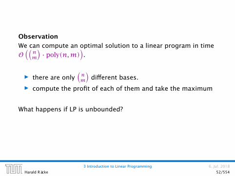
Observation
We can compute an optimal solution to a linear program in time
O((nm
)· poly(n,m)
).
ñ there are only(nm
)different bases.
ñ compute the profit of each of them and take the maximum
What happens if LP is unbounded?
3 Introduction to Linear Programming 6. Jul. 2018
Harald Räcke 52/554

4 Simplex Algorithm
Enumerating all basic feasible solutions (BFS), in order to find
the optimum is slow.
Simplex Algorithm [George Dantzig 1947]
Move from BFS to adjacent BFS, without decreasing objective
function.
Two BFSs are called adjacent if the bases just differ in one
variable.
4 Simplex Algorithm 6. Jul. 2018
Harald Räcke 53/554

4 Simplex Algorithm
max 13a + 23b
s.t. 5a + 15b + sc = 480
4a + 4b + sh = 160
35a + 20b + sm = 1190
a , b , sc , sh , sm ≥ 0
max Z13a + 23b − Z = 0
5a + 15b + sc = 480
4a + 4b + sh = 160
35a + 20b + sm = 1190
a , b , sc , sh , sm ≥ 0
basis = sc , sh, sma = b = 0Z = 0
sc = 480sh = 160sm= 1190
4 Simplex Algorithm 6. Jul. 2018
Harald Räcke 54/554

Pivoting Step
max Z13a + 23b − Z = 0
5a + 15b + sc = 480
4a + 4b + sh = 160
35a + 20b + sm = 1190
a , b , sc , sh , sm ≥ 0
basis = sc , sh, sma = b = 0Z = 0
sc = 480sh = 160sm= 1190
ñ choose variable to bring into the basis
ñ chosen variable should have positive coefficient in objective
function
ñ apply min-ratio test to find out by how much the variable
can be increased
ñ pivot on row found by min-ratio test
ñ the existing basis variable in this row leaves the basis
max Z13a + 23b − Z = 0
5a + 15b + sc = 480
4a + 4b + sh = 160
35a + 20b + sm = 1190
a , b , sc , sh , sm ≥ 0
basis = sc , sh, sma = b = 0Z = 0
sc = 480sh = 160sm= 1190
b
bbbb
scb
ñ Choose variable with coefficient > 0 as entering variable.
ñ If we keep a = 0 and increase b from 0 to θ > 0 s.t. all
constraints (Ax = b,x ≥ 0) are still fulfilled the objective
value Z will strictly increase.
ñ For maintaining Ax = b we need e.g. to set sc = 480− 15θ.
ñ Choosing θ =min480/15, 160/4, 1190/20 ensures that in the
new solution one current basic variable becomes 0, and no
variable goes negative.
ñ The basic variable in the row that gives
min480/15, 160/4, 1190/20 becomes the leaving variable.

max Z13a + 23b − Z = 0
5a + 15b + sc = 480
4a + 4b + sh = 160
35a + 20b + sm = 1190
a , b , sc , sh , sm ≥ 0
basis = sc , sh, sma = b = 0Z = 0
sc = 480sh = 160sm= 1190
b
bbbb
Substitute b = 115(480− 5a− sc).
max Z163 a − 23
15sc − Z = −73613a + b + 1
15sc = 3283a − 4
15sc + sh = 32853 a − 4
3sc + sm = 550
a , b , sc , sh , sm ≥ 0
basis = b, sh, sma = sc = 0Z = 736
b = 32sh = 32sm= 550
max Z163 a − 23
15sc − Z = −73613a + b + 1
15sc = 3283a − 4
15sc + sh = 32853 a − 4
3sc + sm = 550
a , b , sc , sh , sm ≥ 0
basis = b, sh, sma = sc = 0Z = 736
b = 32sh = 32sm= 550
a
a
a
a
a
a
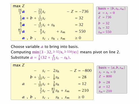
Choose variable a to bring into basis.
Computing min3 · 32, 3·32/8, 3·550/85 means pivot on line 2.
Substitute a = 38(32+ 4
15sc − sh).max Z
− sc − 2sh − Z = −800
b + 110sc − 1
8sh = 28
a − 110sc + 3
8sh = 1232sc − 85
8 sh + sm = 210
a , b , sc , sh , sm ≥ 0
basis = a,b, smsc = sh = 0Z = 800
b = 28a = 12sm= 210

4 Simplex Algorithm
Pivoting stops when all coefficients in the objective function are
non-positive.
Solution is optimal:
ñ any feasible solution satisfies all equations in the tableaux
ñ in particular: Z = 800− sc − 2sh, sc ≥ 0, sh ≥ 0
ñ hence optimum solution value is at most 800
ñ the current solution has value 800
4 Simplex Algorithm 6. Jul. 2018
Harald Räcke 59/554

Matrix ViewLet our linear program be
cTBxB + cTNxN = ZABxB + ANxN = bxB , xN ≥ 0
The simplex tableaux for basis B is
(cTN − cTBA−1B AN)xN = Z − cTBA−1
B bIxB + A−1
B ANxN = A−1B b
xB , xN ≥ 0
The BFS is given by xN = 0, xB = A−1B b.
If (cTN − cTBA−1B AN) ≤ 0 we know that we have an optimum
solution.
4 Simplex Algorithm 6. Jul. 2018
Harald Räcke 60/554

Geometric View of Pivoting
hops
malt
corn
ale
bee
r
a, sc , sh
b, sh, sm
a, b, sm
sc , sh, sm
a, b, sc
max 13a + 23b
s.t. 5a + 15b + sc = 480
4a + 4b + sh = 160
35a + 20b + sm = 1190
a , b , sc , sh , sm ≥ 0

Algebraic Definition of Pivoting
ñ Given basis B with BFS x∗.
ñ Choose index j ∉ B in order to increase x∗j from 0 to θ > 0.ñ Other non-basis variables should stay at 0.ñ Basis variables change to maintain feasibility.
ñ Go from x∗ to x∗ + θ · d.
Requirements for d:
ñ dj = 1 (normalization)
ñ d` = 0, ` ∉ B, ` ≠ jñ A(x∗ + θd) = b must hold. Hence Ad = 0.
ñ Altogether: ABdB +A∗j = Ad = 0, which gives
dB = −A−1B A∗j.
4 Simplex Algorithm 6. Jul. 2018
Harald Räcke 62/554

Algebraic Definition of Pivoting
Definition 26 (j-th basis direction)
Let B be a basis, and let j ∉ B. The vector d with dj = 1 and
d` = 0, ` ∉ B, ` ≠ j and dB = −A−1B A∗j is called the j-th basis
direction for B.
Going from x∗ to x∗ + θ · d the objective function changes by
θ · cTd = θ(cj − cTBA−1B A∗j)
4 Simplex Algorithm 6. Jul. 2018
Harald Räcke 63/554

Algebraic Definition of Pivoting
Definition 27 (Reduced Cost)
For a basis B the value
cj = cj − cTBA−1B A∗j
is called the reduced cost for variable xj.
Note that this is defined for every j. If j ∈ B then the above term
is 0.
4 Simplex Algorithm 6. Jul. 2018
Harald Räcke 64/554

Algebraic Definition of PivotingLet our linear program be
cTBxB + cTNxN = ZABxB + ANxN = bxB , xN ≥ 0
The simplex tableaux for basis B is
(cTN − cTBA−1B AN)xN = Z − cTBA−1
B bIxB + A−1
B ANxN = A−1B b
xB , xN ≥ 0
The BFS is given by xN = 0, xB = A−1B b.
If (cTN − cTBA−1B AN) ≤ 0 we know that we have an optimum
solution.
4 Simplex Algorithm 6. Jul. 2018
Harald Räcke 65/554

4 Simplex Algorithm
Questions:
ñ What happens if the min ratio test fails to give us a value θby which we can safely increase the entering variable?
ñ How do we find the initial basic feasible solution?
ñ Is there always a basis B such that
(cTN − cTBA−1B AN) ≤ 0 ?
Then we can terminate because we know that the solution is
optimal.
ñ If yes how do we make sure that we reach such a basis?
4 Simplex Algorithm 6. Jul. 2018
Harald Räcke 66/554

Min Ratio Test
The min ratio test computes a value θ ≥ 0 such that after setting
the entering variable to θ the leaving variable becomes 0 and all
other variables stay non-negative.
For this, one computes bi/Aie for all constraints i and calculates
the minimum positive value.
What does it mean that the ratio bi/Aie (and hence Aie) is
negative for a constraint?
This means that the corresponding basic variable will increase if
we increase b. Hence, there is no danger of this basic variable
becoming negative
What happens if all bi/Aie are negative? Then we do not have a
leaving variable. Then the LP is unbounded!

Termination
The objective function does not decrease during one iteration of
the simplex-algorithm.
Does it always increase?
4 Simplex Algorithm 6. Jul. 2018
Harald Räcke 68/554

Termination
The objective function may not increase!
Because a variable x` with ` ∈ B is already 0.
The set of inequalities is degenerate (also the basis is
degenerate).
Definition 28 (Degeneracy)
A BFS x∗ is called degenerate if the set J = j | x∗j > 0 fulfills
|J| <m.
It is possible that the algorithm cycles, i.e., it cycles through a
sequence of different bases without ever terminating. Happens,
very rarely in practise.
4 Simplex Algorithm 6. Jul. 2018
Harald Räcke 69/554

Non Degenerate Example
hops
malt
corn
ale
bee
r
max 13a + 23b
s.t. 5a + 15b + sc = 480
4a + 4b + sh = 160
35a + 20b + sm = 1190
a , b , sc , sh , sm ≥ 0

Degenerate Example
hops
malt
corn
ale
bee
rpro
fit
a-direc.
b-d
irec.
pro
fit
sm-direc.
b-d
irec. pro
fit
sh -d
irec.
sm-direc.
pro
fit
sc -direc.
sh -direc.
a, sc , sh
a, b, sm
sc , sh, sma, b, sc
max 13a + 23b
s.t. 5a + 15b + sc = 480
80/17 · a + 4b + sh = 160
35a + 20b + sm = 1190
a , b , sc , sh , sm ≥ 0

Summary: How to choose pivot-elements
ñ We can choose a column e as an entering variable if ce > 0
(ce is reduced cost for xe).ñ The standard choice is the column that maximizes ce.ñ If Aie ≤ 0 for all i ∈ 1, . . . ,m then the maximum is not
bounded.
ñ Otw. choose a leaving variable ` such that b`/A`e is
minimal among all variables i with Aie > 0.
ñ If several variables have minimum b`/A`e you reach a
degenerate basis.
ñ Depending on the choice of ` it may happen that the
algorithm runs into a cycle where it does not escape from a
degenerate vertex.
4 Simplex Algorithm 6. Jul. 2018
Harald Räcke 72/554

Termination
What do we have so far?
Suppose we are given an initial feasible solution to an LP. If the
LP is non-degenerate then Simplex will terminate.
Note that we either terminate because the min-ratio test fails
and we can conclude that the LP is unbounded, or we terminate
because the vector of reduced cost is non-positive. In the latter
case we have an optimum solution.
4 Simplex Algorithm 6. Jul. 2018
Harald Räcke 73/554

How do we come up with an initial solution?
ñ Ax ≤ b,x ≥ 0, and b ≥ 0.
ñ The standard slack form for this problem is
Ax + Is = b,x ≥ 0, s ≥ 0, where s denotes the vector of
slack variables.
ñ Then s = b, x = 0 is a basic feasible solution (how?).
ñ We directly can start the simplex algorithm.
How do we find an initial basic feasible solution for an arbitrary
problem?
4 Simplex Algorithm 6. Jul. 2018
Harald Räcke 74/554

Two phase algorithm
Suppose we want to maximize cTx s.t. Ax = b,x ≥ 0.
1. Multiply all rows with bi < 0 by −1.
2. maximize −∑i vi s.t. Ax + Iv = b, x ≥ 0, v ≥ 0 using
Simplex. x = 0, v = b is initial feasible.
3. If∑i vi > 0 then the original problem is infeasible.
4. Otw. you have x ≥ 0 with Ax = b.
5. From this you can get basic feasible solution.
6. Now you can start the Simplex for the original problem.
4 Simplex Algorithm 6. Jul. 2018
Harald Räcke 75/554

Optimality
Lemma 29
Let B be a basis and x∗ a BFS corresponding to basis B. c ≤ 0
implies that x∗ is an optimum solution to the LP.
4 Simplex Algorithm 6. Jul. 2018
Harald Räcke 76/554

Duality
How do we get an upper bound to a maximization LP?
max 13a + 23b
s.t. 5a + 15b ≤ 480
4a + 4b ≤ 160
35a + 20b ≤ 1190
a,b ≥ 0
Note that a lower bound is easy to derive. Every choice of
a,b ≥ 0 gives us a lower bound (e.g. a = 12, b = 28 gives us a
lower bound of 800).
If you take a conic combination of the rows (multiply the i-th row
with yi ≥ 0) such that∑iyiaij ≥ cj then
∑iyibi will be an
upper bound.
5.1 Weak Duality 6. Jul. 2018
Harald Räcke 77/554

Duality
Definition 30
Let z =maxcTx | Ax ≤ b,x ≥ 0 be a linear program P (called
the primal linear program).
The linear program D defined by
w =minbTy | ATy ≥ c,y ≥ 0
is called the dual problem.
5.1 Weak Duality 6. Jul. 2018
Harald Räcke 78/554

Duality
Lemma 31
The dual of the dual problem is the primal problem.
Proof:
ñ w =minbTy | ATy ≥ c,y ≥ 0ñ w = −max−bTy | −ATy ≤ −c,y ≥ 0
The dual problem is
ñ z = −min−cTx | −Ax ≥ −b,x ≥ 0ñ z =maxcTx | Ax ≤ b,x ≥ 0
5.1 Weak Duality 6. Jul. 2018
Harald Räcke 79/554

Weak Duality
Let z =maxcTx | Ax ≤ b,x ≥ 0 and
w =minbTy | ATy ≥ c,y ≥ 0 be a primal dual pair.
x is primal feasible iff x ∈ x | Ax ≤ b,x ≥ 0
y is dual feasible, iff y ∈ y | ATy ≥ c,y ≥ 0.
Theorem 32 (Weak Duality)
Let x be primal feasible and let y be dual feasible. Then
cT x ≤ z ≤ w ≤ bT y .
5.1 Weak Duality 6. Jul. 2018
Harald Räcke 80/554
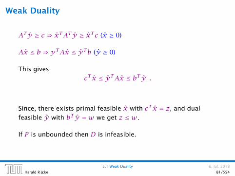
Weak Duality
AT y ≥ c ⇒ xTAT y ≥ xTc (x ≥ 0)
Ax ≤ b ⇒ yTAx ≤ yTb (y ≥ 0)
This gives
cT x ≤ yTAx ≤ bT y .
Since, there exists primal feasible x with cT x = z, and dual
feasible y with bT y = w we get z ≤ w.
If P is unbounded then D is infeasible.
5.1 Weak Duality 6. Jul. 2018
Harald Räcke 81/554

5.2 Simplex and Duality
The following linear programs form a primal dual pair:
z =maxcTx | Ax = b,x ≥ 0w =minbTy | ATy ≥ c
This means for computing the dual of a standard form LP, we do
not have non-negativity constraints for the dual variables.
5.2 Simplex and Duality 6. Jul. 2018
Harald Räcke 82/554

Proof
Primal:
maxcTx | Ax = b,x ≥ 0=maxcTx | Ax ≤ b,−Ax ≤ −b,x ≥ 0
=maxcTx |[A−A
]x ≤
[b−b
], x ≥ 0
Dual:
min[bT −bT ]y | [AT −AT ]y ≥ c,y ≥ 0
=min
[bT −bT ] ·
[y+
y−
]∣∣∣∣∣[AT −AT ] ·
[y+
y−
]≥ c,y− ≥ 0, y+ ≥ 0
=minbT · (y+ −y−)
∣∣∣AT · (y+ −y−) ≥ c,y− ≥ 0, y+ ≥ 0
=minbTy ′
∣∣∣ATy ′ ≥ c
5.2 Simplex and Duality 6. Jul. 2018
Harald Räcke 83/554

Proof of Optimality Criterion for Simplex
Suppose that we have a basic feasible solution with reduced cost
c = cT − cTBA−1B A ≤ 0
This is equivalent to AT (A−1B )TcB ≥ c
y∗ = (A−1B )TcB is solution to the dual minbTy|ATy ≥ c.
bTy∗ = (Ax∗)Ty∗ = (ABx∗B )Ty∗= (ABx∗B )T (A−1
B )TcB = (x∗B )TATB (A−1
B )TcB
= cTx∗
Hence, the solution is optimal.
5.2 Simplex and Duality 6. Jul. 2018
Harald Räcke 84/554

5.3 Strong Duality
P =maxcTx | Ax ≤ b,x ≥ 0nA: number of variables, mA: number of constraints
We can put the non-negativity constraints into A (which gives us
unrestricted variables): P =maxcTx | Ax ≤ bnA = nA, mA =mA +nA
Dual D =minbTy | ATy = c,y ≥ 0.
5.3 Strong Duality 6. Jul. 2018
Harald Räcke 85/554

5.3 Strong Duality
hops
malt
corn
ale
bee
r
pro
fitc
a, b, sm
The profit vector c lies in the cone generated by the normals for
the hops and the corn constraint (the tight constraints).
If we have a conic combination y of c thenbTy is an upper bound of the profit we canobtain (weak duality):
cTx = (ATy)Tx = yT Ax ≤ yT bIf x and y are optimal then the duality gapis 0 (strong duality). This means
0 = cTx −yT b= (ATy)Tx −yT b= yT (Ax − b)
The last term can only be 0 if yi is 0 when-ever the i-th constraint is not tight. Thismeans we have a conic combination of cby normals (columns of AT ) of tight con-straints.
Conversely, if we have x such that the nor-mals of tight constraint (at x) give rise to aconic combination of c, we know that x isoptimal.

Strong Duality
Theorem 33 (Strong Duality)
Let P and D be a primal dual pair of linear programs, and let z∗
and w∗ denote the optimal solution to P and D, respectively.
Then
z∗ = w∗
5.3 Strong Duality 6. Jul. 2018
Harald Räcke 87/554

Lemma 34 (Weierstrass)
Let X be a compact set and let f(x) be a continuous function on
X. Then minf(x) : x ∈ X exists.
(without proof)
5.3 Strong Duality 6. Jul. 2018
Harald Räcke 88/554

Lemma 35 (Projection Lemma)
Let X ⊆ Rm be a non-empty convex set, and let y ∉ X. Then
there exist x∗ ∈ X with minimum distance from y. Moreover for
all x ∈ X we have (y − x∗)T (x − x∗) ≤ 0.
y
x∗
x′
5.3 Strong Duality 6. Jul. 2018
Harald Räcke 89/554

Proof of the Projection Lemmañ Define f(x) = ‖y − x‖.ñ We want to apply Weierstrass but X may not be bounded.ñ X ≠ . Hence, there exists x′ ∈ X.ñ Define X′ = x ∈ X | ‖y − x‖ ≤ ‖y − x′‖. This set is
closed and bounded.ñ Applying Weierstrass gives the existence.
y
x∗
x′
5.3 Strong Duality 6. Jul. 2018
Harald Räcke 90/554
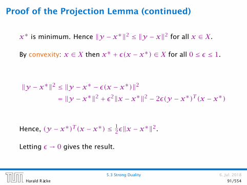
Proof of the Projection Lemma (continued)
x∗ is minimum. Hence ‖y − x∗‖2 ≤ ‖y − x‖2 for all x ∈ X.
By convexity: x ∈ X then x∗ + ε(x − x∗) ∈ X for all 0 ≤ ε ≤ 1.
‖y − x∗‖2 ≤ ‖y − x∗ − ε(x − x∗)‖2
= ‖y − x∗‖2 + ε2‖x − x∗‖2 − 2ε(y − x∗)T (x − x∗)
Hence, (y − x∗)T (x − x∗) ≤ 12ε‖x − x∗‖2.
Letting ε → 0 gives the result.
5.3 Strong Duality 6. Jul. 2018
Harald Räcke 91/554
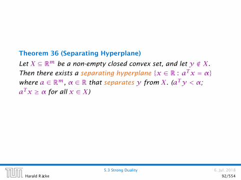
Theorem 36 (Separating Hyperplane)
Let X ⊆ Rm be a non-empty closed convex set, and let y ∉ X.
Then there exists a separating hyperplane x ∈ R : aTx = αwhere a ∈ Rm, α ∈ R that separates y from X. (aTy < α;
aTx ≥ α for all x ∈ X)
5.3 Strong Duality 6. Jul. 2018
Harald Räcke 92/554

Proof of the Hyperplane Lemma
ñ Let x∗ ∈ X be closest point to y in X.
ñ By previous lemma (y − x∗)T (x − x∗) ≤ 0 for all x ∈ X.
ñ Choose a = (x∗ −y) and α = aTx∗.
ñ For x ∈ X : aT (x − x∗) ≥ 0, and, hence, aTx ≥ α.
ñ Also, aTy = aT (x∗ − a) = α− ‖a‖2 < α
H = x | aTx = α
y
x∗
x
5.3 Strong Duality 6. Jul. 2018
Harald Räcke 93/554

Lemma 37 (Farkas Lemma)
Let A be an m×n matrix, b ∈ Rm. Then exactly one of the
following statements holds.
1. ∃x ∈ Rn with Ax = b, x ≥ 0
2. ∃y ∈ Rm with ATy ≥ 0, bTy < 0
Assume x satisfies 1. and y satisfies 2. Then
0 > yTb = yTAx ≥ 0
Hence, at most one of the statements can hold.
5.3 Strong Duality 6. Jul. 2018
Harald Räcke 94/554

Farkas Lemma
b
y
a1
a2
a3
a4
If b is not in the cone generated by the columns of A, there
exists a hyperplane y that separates b from the cone.

Proof of Farkas Lemma
Now, assume that 1. does not hold.
Consider S = Ax : x ≥ 0 so that S closed, convex, b ∉ S.
We want to show that there is y with ATy ≥ 0, bTy < 0.
Let y be a hyperplane that separates b from S. Hence, yTb < αand yT s ≥ α for all s ∈ S.
0 ∈ S ⇒ α ≤ 0⇒ yTb < 0
yTAx ≥ α for all x ≥ 0. Hence, yTA ≥ 0 as we can choose xarbitrarily large.
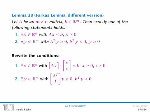
Lemma 38 (Farkas Lemma; different version)
Let A be an m×n matrix, b ∈ Rm. Then exactly one of the
following statements holds.
1. ∃x ∈ Rn with Ax ≤ b, x ≥ 0
2. ∃y ∈ Rm with ATy ≥ 0, bTy < 0, y ≥ 0
Rewrite the conditions:
1. ∃x ∈ Rn with[A I
]·[xs
]= b, x ≥ 0, s ≥ 0
2. ∃y ∈ Rm with
[AT
I
]y ≥ 0, bTy < 0
5.3 Strong Duality 6. Jul. 2018
Harald Räcke 97/554

Proof of Strong Duality
P : z =maxcTx | Ax ≤ b,x ≥ 0
D: w =minbTy | ATy ≥ c,y ≥ 0
Theorem 39 (Strong Duality)
Let P and D be a primal dual pair of linear programs, and let zand w denote the optimal solution to P and D, respectively (i.e.,
P and D are non-empty). Then
z = w .
5.3 Strong Duality 6. Jul. 2018
Harald Räcke 98/554

Proof of Strong Duality
z ≤ w: follows from weak duality
z ≥ w:
We show z < α implies w < α.
∃x ∈ Rn
s.t. Ax ≤ b−cTx ≤ −α
x ≥ 0
∃y ∈ Rm;v ∈ Rs.t. ATy − cv ≥ 0
bTy −αv < 0
y,v ≥ 0
∃y ∈ Rm;v ∈ Rs.t. ATy − cv ≥ 0
bTy −αv < 0
y,v ≥ 0
From the definition of α we know that the first system is
infeasible; hence the second must be feasible.
5.3 Strong Duality 6. Jul. 2018
Harald Räcke 99/554

Proof of Strong Duality
∃y ∈ Rm;v ∈ Rs.t. ATy − cv ≥ 0
bTy −αv < 0
y,v ≥ 0
If the solution y,v has v = 0 we have that
∃y ∈ Rm
s.t. ATy ≥ 0
bTy < 0
y ≥ 0
is feasible. By Farkas lemma this gives that LP P is infeasible.
Contradiction to the assumption of the lemma.
5.3 Strong Duality 6. Jul. 2018
Harald Räcke 100/554

Proof of Strong Duality
Hence, there exists a solution y,v with v > 0.
We can rescale this solution (scaling both y and v) s.t. v = 1.
Then y is feasible for the dual but bTy < α. This means that
w < α.
5.3 Strong Duality 6. Jul. 2018
Harald Räcke 101/554
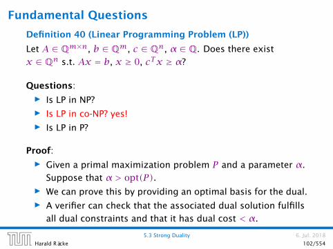
Fundamental Questions
Definition 40 (Linear Programming Problem (LP))
Let A ∈ Qm×n, b ∈ Qm, c ∈ Qn, α ∈ Q. Does there exist
x ∈ Qn s.t. Ax = b, x ≥ 0, cTx ≥ α?
Questions:
ñ Is LP in NP?
ñ Is LP in co-NP? yes!
ñ Is LP in P?
Proof:
ñ Given a primal maximization problem P and a parameter α.
Suppose that α > opt(P).ñ We can prove this by providing an optimal basis for the dual.
ñ A verifier can check that the associated dual solution fulfills
all dual constraints and that it has dual cost < α.
5.3 Strong Duality 6. Jul. 2018
Harald Räcke 102/554
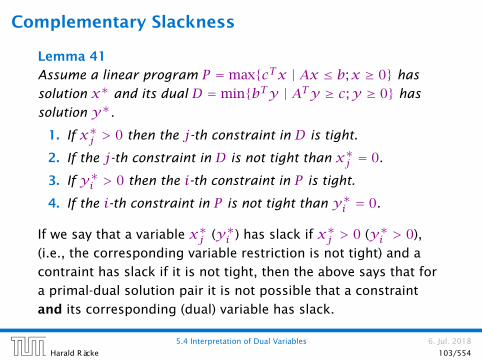
Complementary Slackness
Lemma 41
Assume a linear program P =maxcTx | Ax ≤ b;x ≥ 0 has
solution x∗ and its dual D =minbTy | ATy ≥ c;y ≥ 0 has
solution y∗.
1. If x∗j > 0 then the j-th constraint in D is tight.
2. If the j-th constraint in D is not tight than x∗j = 0.
3. If y∗i > 0 then the i-th constraint in P is tight.
4. If the i-th constraint in P is not tight than y∗i = 0.
If we say that a variable x∗j (y∗i ) has slack if x∗j > 0 (y∗i > 0),
(i.e., the corresponding variable restriction is not tight) and a
contraint has slack if it is not tight, then the above says that for
a primal-dual solution pair it is not possible that a constraint
and its corresponding (dual) variable has slack.
5.4 Interpretation of Dual Variables 6. Jul. 2018
Harald Räcke 103/554

Proof: Complementary SlacknessAnalogous to the proof of weak duality we obtain
cTx∗ ≤ y∗TAx∗ ≤ bTy∗
Because of strong duality we then get
cTx∗ = y∗TAx∗ = bTy∗
This gives e.g. ∑
j(yTA− cT )jx∗j = 0
From the constraint of the dual it follows that yTA ≥ cT . Hence
the left hand side is a sum over the product of non-negative
numbers. Hence, if e.g. (yTA− cT )j > 0 (the j-th constraint in
the dual is not tight) then xj = 0 (2.). The result for (1./3./4.)
follows similarly.
5.4 Interpretation of Dual Variables 6. Jul. 2018
Harald Räcke 104/554

Interpretation of Dual Variables
ñ Brewer: find mix of ale and beer that maximizes profits
max 13a + 23bs.t. 5a + 15b ≤ 480
4a + 4b ≤ 16035a + 20b ≤ 1190
a,b ≥ 0
ñ Entrepeneur: buy resources from brewer at minimum costC, H, M: unit price for corn, hops and malt.
min 480C + 160H + 1190Ms.t. 5C + 4H + 35M ≥ 13
15C + 4H + 20M ≥ 23C,H,M ≥ 0
Note that brewer won’t sell (at least not all) if e.g.5C +4H+35M < 13 as then brewing ale would be advantageous.

Interpretation of Dual Variables
Marginal Price:
ñ How much money is the brewer willing to pay for additional
amount of Corn, Hops, or Malt?
ñ We are interested in the marginal price, i.e., what happens if
we increase the amount of Corn, Hops, and Malt by εC , εH ,
and εM , respectively.
The profit increases to maxcTx | Ax ≤ b+ ε;x ≥ 0. Because of
strong duality this is equal to
min (bT + εT )ys.t. ATy ≥ c
y ≥ 0
5.4 Interpretation of Dual Variables 6. Jul. 2018
Harald Räcke 106/554

Interpretation of Dual Variables
If ε is “small” enough then the optimum dual solution y∗ might
not change. Therefore the profit increases by∑i εiy∗i .
Therefore we can interpret the dual variables as marginal prices.
Note that with this interpretation, complementary slackness
becomes obvious.
ñ If the brewer has slack of some resource (e.g. corn) then he
is not willing to pay anything for it (corresponding dual
variable is zero).
ñ If the dual variable for some resource is non-zero, then an
increase of this resource increases the profit of the brewer.
Hence, it makes no sense to have left-overs of this resource.
Therefore its slack must be zero.
5.4 Interpretation of Dual Variables 6. Jul. 2018
Harald Räcke 107/554

Example
hops
malt
corn
ale
bee
r
pro
fit
sc -direc.
sh -direc.a, b, sm
The change in profit when increasing hops by one unit is
= cTBA−1B eh.cTBA−1B︸ ︷︷ ︸
y∗
max 13a + 23b
s.t. 5a + 15b + sc = 480
4a + 4b + sh = 160
35a + 20b + sm = 1190
a , b , sc , sh , sm ≥ 0

Of course, the previous argument about the increase in the
primal objective only holds for the non-degenerate case.
If the optimum basis is degenerate then increasing the supply of
one resource may not allow the objective value to increase.
5.4 Interpretation of Dual Variables 6. Jul. 2018
Harald Räcke 109/554

Flows
Definition 42
An (s, t)-flow in a (complete) directed graph G = (V , V × V, c) is
a function f : V × V , R+0 that satisfies
1. For each edge (x,y)
0 ≤ fxy ≤ cxy .
(capacity constraints)
2. For each v ∈ V \ s, t∑xfvx =
∑xfxv .
(flow conservation constraints)
5.5 Computing Duals 6. Jul. 2018
Harald Räcke 110/554

Flows
Definition 43
The value of an (s, t)-flow f is defined as
val(f ) =∑xfsx −
∑xfxs .
Maximum Flow Problem:
Find an (s, t)-flow with maximum value.
5.5 Computing Duals 6. Jul. 2018
Harald Räcke 111/554

LP-Formulation of Maxflow
max∑z fsz −
∑z fzs
s.t. ∀(z,w) ∈ V × V fzw ≤ czw `zw∀w ≠ s, t
∑z fzw −
∑z fwz = 0 pwfzw ≥ 0
min∑(xy) cxy`xy
s.t. fxy (x,y ≠ s, t) : 1`xy−1px+1py ≥ 0
fsy (y ≠ s, t) : 1`sy +1py ≥ 1
fxs (x ≠ s, t) : 1`xs−1px ≥ −1
fty (y ≠ s, t) : 1`ty +1py ≥ 0
fxt (x ≠ s, t) : 1`xt−1px ≥ 0
fst : 1`st ≥ 1
fts : 1`ts ≥ −1
`xy ≥ 0
5.5 Computing Duals 6. Jul. 2018
Harald Räcke 112/554

LP-Formulation of Maxflow
min∑(xy) cxy`xy
s.t. fxy (x,y ≠ s, t) : 1`xy−1px+1py ≥ 0
fsy (y ≠ s, t) : 1`sy− 1+1py ≥ 0
fxs (x ≠ s, t) : 1`xs−1px+ 1 ≥ 0
fty (y ≠ s, t) : 1`ty− 0+1py ≥ 0
fxt (x ≠ s, t) : 1`xt−1px+ 0 ≥ 0
fst : 1`st− 1+ 0 ≥ 0
fts : 1`ts− 0+ 1 ≥ 0
`xy ≥ 0
5.5 Computing Duals 6. Jul. 2018
Harald Räcke 113/554

LP-Formulation of Maxflow
min∑(xy) cxy`xy
s.t. fxy (x,y ≠ s, t) : 1`xy−1px+1py ≥ 0
fsy (y ≠ s, t) : 1`sy− ps+1py ≥ 0
fxs (x ≠ s, t) : 1`xs−1px+ ps ≥ 0
fty (y ≠ s, t) : 1`ty− pt+1py ≥ 0
fxt (x ≠ s, t) : 1`xt−1px+ pt ≥ 0
fst : 1`st− ps+ pt ≥ 0
fts : 1`ts− pt+ ps ≥ 0
`xy ≥ 0
with pt = 0 and ps = 1.
5.5 Computing Duals 6. Jul. 2018
Harald Räcke 114/554
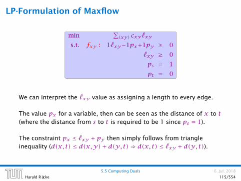
LP-Formulation of Maxflow
min∑(xy) cxy`xy
s.t. fxy : 1`xy−1px+1py ≥ 0
`xy ≥ 0
ps = 1
pt = 0
We can interpret the `xy value as assigning a length to every edge.
The value px for a variable, then can be seen as the distance of x to t(where the distance from s to t is required to be 1 since ps = 1).
The constraint px ≤ `xy + py then simply follows from triangleinequality (d(x, t) ≤ d(x,y)+ d(y, t)⇒ d(x, t) ≤ `xy + d(y, t)).
5.5 Computing Duals 6. Jul. 2018
Harald Räcke 115/554

One can show that there is an optimum LP-solution for the dual
problem that gives an integral assignment of variables.
This means px = 1 or px = 0 for our case. This gives rise to a
cut in the graph with vertices having value 1 on one side and the
other vertices on the other side. The objective function then
evaluates the capacity of this cut.
This shows that the Maxflow/Mincut theorem follows from linear
programming duality.
5.5 Computing Duals 6. Jul. 2018
Harald Räcke 116/554

Degeneracy Revisited
If a basis variable is 0 in the basic feasible solution then we may
not make progress during an iteration of simplex.
Idea:
Change LP :=maxcTx,Ax = b;x ≥ 0 into
LP′ :=maxcTx,Ax = b′, x ≥ 0 such that
I. LP is feasible
II. If a set B of basis variables corresponds to an infeasible
basis (i.e. A−1B b 6≥ 0) then B corresponds to an infeasible
basis in LP′ (note that columns in AB are linearly
independent).
III. LP has no degenerate basic solutions
6 Degeneracy Revisited 6. Jul. 2018
Harald Räcke 117/554

Degenerate Example
hops
malt
corn
ale
bee
rpro
fit
a-direc.
b-d
irec.
pro
fit
sm-direc.
b-d
irec. pro
fit
sh -d
irec.
sm-direc.
pro
fit
sc -direc.
sh -direc.
a, sc , sh
a, b, sm
sc , sh, sma, b, sc
max 13a + 23b
s.t. 5a + 15b + sc = 480
80/17 · a + 4b + sh = 160
35a + 20b + sm = 1190
a , b , sc , sh , sm ≥ 0

Degeneracy Revisited
If a basis variable is 0 in the basic feasible solution then we may
not make progress during an iteration of simplex.
Idea:
Given feasible LP :=maxcTx,Ax = b;x ≥ 0. Change it into
LP′ :=maxcTx,Ax = b′, x ≥ 0 such that
I. LP′ is feasible
II. If a set B of basis variables corresponds to an infeasible
basis (i.e. A−1B b 6≥ 0) then B corresponds to an infeasible
basis in LP′ (note that columns in AB are linearly
independent).
III. LP′ has no degenerate basic solutions
6 Degeneracy Revisited 6. Jul. 2018
Harald Räcke 119/554

Perturbation
Let B be index set of some basis with basic solution
x∗B = A−1B b ≥ 0, x∗N = 0 (i.e. B is feasible)
Fix
b′ := b +AB
ε...
εm
for ε > 0 .
This is the perturbation that we are using.
6 Degeneracy Revisited 6. Jul. 2018
Harald Räcke 120/554

Property I
The new LP is feasible because the set B of basis variables
provides a feasible basis:
A−1B
b +AB
ε...
εm
= x∗B +
ε...
εm
≥ 0 .
6 Degeneracy Revisited 6. Jul. 2018
Harald Räcke 121/554

Property II
Let B be a non-feasible basis. This means (A−1B b)i < 0 for some
row i.
Then for small enough ε > 0
A−1
B
b +AB
ε...
εm
i
= (A−1B b)i +
A−1
B AB
ε...
εm
i
< 0
Hence, B is not feasible.
6 Degeneracy Revisited 6. Jul. 2018
Harald Räcke 122/554

Property IIILet B be a basis. It has an associated solution
x∗B = A−1B b +A−1
B AB
ε...
εm
in the perturbed instance.
We can view each component of the vector as a polynom with
variable ε of degree at most m.
A−1B AB has rank m. Therefore no polynom is 0.
A polynom of degree at most m has at most m roots
(Nullstellen).
Hence, ε > 0 small enough gives that no component of the
above vector is 0. Hence, no degeneracies.
6 Degeneracy Revisited 6. Jul. 2018
Harald Räcke 123/554

Since, there are no degeneracies Simplex will terminate when
run on LP′.ñ If it terminates because the reduced cost vector fulfills
c = (cT − cTBA−1B A) ≤ 0
then we have found an optimal basis. Note that this basis is
also optimal for LP, as the above constraint does not
depend on b.
ñ If it terminates because it finds a variable xj with cj > 0 for
which the j-th basis direction d, fulfills d ≥ 0 we know that
LP′ is unbounded. The basis direction does not depend on
b. Hence, we also know that LP is unbounded.
6 Degeneracy Revisited 6. Jul. 2018
Harald Räcke 124/554
Lexicographic Pivoting
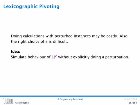
Doing calculations with perturbed instances may be costly. Also
the right choice of ε is difficult.
Idea:
Simulate behaviour of LP′ without explicitly doing a perturbation.
6 Degeneracy Revisited 6. Jul. 2018
Harald Räcke 125/554

Lexicographic Pivoting
We choose the entering variable arbitrarily as before (ce > 0, of
course).
If we do not have a choice for the leaving variable then LP′ and
LP do the same (i.e., choose the same variable).
Otherwise we have to be careful.
6 Degeneracy Revisited 6. Jul. 2018
Harald Räcke 126/554
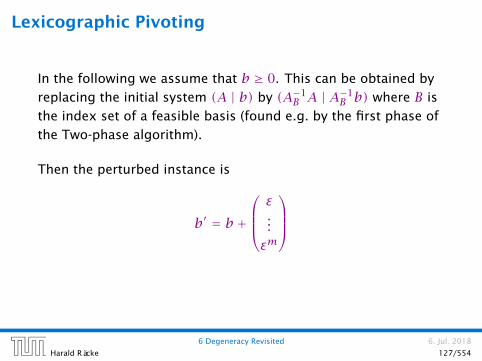
Lexicographic Pivoting
In the following we assume that b ≥ 0. This can be obtained by
replacing the initial system (A | b) by (A−1B A | A−1
B b) where B is
the index set of a feasible basis (found e.g. by the first phase of
the Two-phase algorithm).
Then the perturbed instance is
b′ = b +
ε...
εm
6 Degeneracy Revisited 6. Jul. 2018
Harald Räcke 127/554

Matrix ViewLet our linear program be
cTBxB + cTNxN = ZABxB + ANxN = bxB , xN ≥ 0
The simplex tableaux for basis B is
(cTN − cTBA−1B AN)xN = Z − cTBA−1
B bIxB + A−1
B ANxN = A−1B b
xB , xN ≥ 0
The BFS is given by xN = 0, xB = A−1B b.
If (cTN − cTBA−1B AN) ≤ 0 we know that we have an optimum
solution.
6 Degeneracy Revisited 6. Jul. 2018
Harald Räcke 128/554

Lexicographic Pivoting
LP chooses an arbitrary leaving variable that has A`e > 0 and
minimizes
θ` =b`A`e
= (A−1B b)`
(A−1B A∗e)`
.
` is the index of a leaving variable within B. This means if e.g.
B = 1,3,7,14 and leaving variable is 3 then ` = 2.
6 Degeneracy Revisited 6. Jul. 2018
Harald Räcke 129/554

Lexicographic Pivoting
Definition 44
u ≤lex v if and only if the first component in which u and vdiffer fulfills ui ≤ vi.
6 Degeneracy Revisited 6. Jul. 2018
Harald Räcke 130/554

Lexicographic Pivoting
LP′ chooses an index that minimizes
θ` =
A−1
B
b +
ε...
εm
`
(A−1B A∗e)`
=
A−1B (b | I)
1
ε...
εm
`
(A−1B A∗e)`
= `-th row of A−1B (b | I)
(A−1B A∗e)`
1
ε...
εm
6 Degeneracy Revisited 6. Jul. 2018
Harald Räcke 131/554
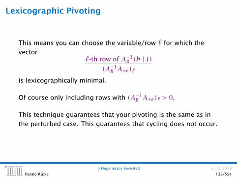
Lexicographic Pivoting
This means you can choose the variable/row ` for which the
vector`-th row of A−1
B (b | I)(A−1B A∗e)`
is lexicographically minimal.
Of course only including rows with (A−1B A∗e)` > 0.
This technique guarantees that your pivoting is the same as in
the perturbed case. This guarantees that cycling does not occur.
6 Degeneracy Revisited 6. Jul. 2018
Harald Räcke 132/554

Number of Simplex Iterations
Each iteration of Simplex can be implemented in polynomial
time.
If we use lexicographic pivoting we know that Simplex requires
at most(nm
)iterations, because it will not visit a basis twice.
The input size is L ·n ·m, where n is the number of variables,
m is the number of constraints, and L is the length of the binary
representation of the largest coefficient in the matrix A.
If we really require(nm
)iterations then Simplex is not a
polynomial time algorithm.
Can we obtain a better analysis?
7 Klee Minty Cube 6. Jul. 2018
Harald Räcke 133/554

Number of Simplex Iterations
Observation
Simplex visits every feasible basis at most once.
However, also the number of feasible bases can be very large.
7 Klee Minty Cube 6. Jul. 2018
Harald Räcke 134/554

Example
max cTxs.t. 0 ≤ x1 ≤ 1
0 ≤ x2 ≤ 1...
0 ≤ xn ≤ 1
x1x2
x3
2n constraint on n variables define an n-dimensional hypercube
as feasible region.
The feasible region has 2n vertices.
7 Klee Minty Cube 6. Jul. 2018
Harald Räcke 135/554

Example
max cTxs.t. 0 ≤ x1 ≤ 1
0 ≤ x2 ≤ 1...
0 ≤ xn ≤ 1
x1x2
x3
However, Simplex may still run quickly as it usually does not
visit all feasible bases.
In the following we give an example of a feasible region for
which there is a bad Pivoting Rule.
7 Klee Minty Cube 6. Jul. 2018
Harald Räcke 136/554

Pivoting Rule
A Pivoting Rule defines how to choose the entering and leaving
variable for an iteration of Simplex.
In the non-degenerate case after choosing the entering variable
the leaving variable is unique.
7 Klee Minty Cube 6. Jul. 2018
Harald Räcke 137/554

Klee Minty Cube
max xns.t. 0 ≤ x1 ≤ 1
εx1 ≤ x2 ≤ 1− εx1
εx2 ≤ x3 ≤ 1− εx2...
εxn−1 ≤ xn ≤ 1− εxn−1
xi ≥ 0
x1x2
x3
(1, ε, ε2)(1, 1 − ε, ε − ε2)
(0, 1, ε)
(0, 1, 1 − ε)
(1, 1 − ε, 1 − ε + ε2)
(1, ε, 1 − ε2)
(0, 0, 1)

Observations
ñ We have 2n constraints, and 3n variables (after adding
slack variables to every constraint).
ñ Every basis is defined by 2n variables, and n non-basic
variables.
ñ There exist degenerate vertices.
ñ The degeneracies come from the non-negativity constraints,
which are superfluous.
ñ In the following all variables xi stay in the basis at all times.
ñ Then, we can uniquely specify a basis by choosing for each
variable whether it should be equal to its lower bound, or
equal to its upper bound (the slack variable corresponding
to the non-tight constraint is part of the basis).
ñ We can also simply identify each basis/vertex with the
corresponding hypercube vertex obtained by letting ε → 0.

Analysis
ñ In the following we specify a sequence of bases (identified
by the corresponding hypercube node) along which the
objective function strictly increases.
ñ The basis (0, . . . ,0,1) is the unique optimal basis.
ñ Our sequence Sn starts at (0, . . . ,0) ends with (0, . . . ,0,1)and visits every node of the hypercube.
ñ An unfortunate Pivoting Rule may choose this sequence,
and, hence, require an exponential number of iterations.
7 Klee Minty Cube 6. Jul. 2018
Harald Räcke 140/554

Klee Minty Cube
max xns.t. 0 ≤ x1 ≤ 1
εx1 ≤ x2 ≤ 1− εx1
εx2 ≤ x3 ≤ 1− εx2
x1x2
x3
(1, ε, ε2)(1, 1 − ε, ε − ε2)
(0, 1, ε)
(0, 1, 1 − ε)
(1, 1 − ε, 1 − ε + ε2)
(1, ε, 1 − ε2)
(0, 0, 1)
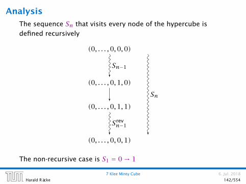
Analysis
The sequence Sn that visits every node of the hypercube is
defined recursively
(0, . . . ,0,0,0)
(0, . . . ,0,1,0)
(0, . . . ,0,1,1)
(0, . . . ,0,0,1)
Sn−1
Srevn−1
Sn
The non-recursive case is S1 = 0→ 1
7 Klee Minty Cube 6. Jul. 2018
Harald Räcke 142/554

Analysis
Lemma 45
The objective value xn is increasing along path Sn.
Proof by induction:
n = 1: obvious, since S1 = 0→ 1, and 1 > 0.
n − 1 → nñ For the first part the value of xn = εxn−1.
ñ By induction hypothesis xn−1 is increasing along Sn−1,
hence, also xn.
ñ Going from (0, . . . ,0,1,0) to (0, . . . ,0,1,1) increases xn for
small enough ε.ñ For the remaining path Srev
n−1 we have xn = 1− εxn−1.
ñ By induction hypothesis xn−1 is increasing along Sn−1,
hence −εxn−1 is increasing along Srevn−1.

Remarks about Simplex
Observation
The simplex algorithm takes at most(nm
)iterations. Each
iteration can be implemented in time O(mn).
In practise it usually takes a linear number of iterations.
7 Klee Minty Cube 6. Jul. 2018
Harald Räcke 144/554
Remarks about Simplex
Theorem
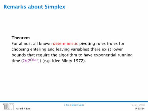
For almost all known deterministic pivoting rules (rules for
choosing entering and leaving variables) there exist lower
bounds that require the algorithm to have exponential running
time (Ω(2Ω(n))) (e.g. Klee Minty 1972).
7 Klee Minty Cube 6. Jul. 2018
Harald Räcke 145/554

Remarks about Simplex
Theorem
For some standard randomized pivoting rules there exist
subexponential lower bounds (Ω(2Ω(nα)) for α > 0) (Friedmann,
Hansen, Zwick 2011).
7 Klee Minty Cube 6. Jul. 2018
Harald Räcke 146/554

Remarks about Simplex
Conjecture (Hirsch 1957)
The edge-vertex graph of an m-facet polytope in d-dimensional
Euclidean space has diameter no more than m− d.
The conjecture has been proven wrong in 2010.
But the question whether the diameter is perhaps of the form
O(poly(m,d)) is open.
7 Klee Minty Cube 6. Jul. 2018
Harald Räcke 147/554

8 Seidels LP-algorithm
ñ Suppose we want to solve mincTx | Ax ≥ b;x ≥ 0, where
x ∈ Rd and we have m constraints.
ñ In the worst-case Simplex runs in time roughly
O(m(m+d)(m+dm
)) ≈ (m+d)m. (slightly better bounds on
the running time exist, but will not be discussed here).
ñ If d is much smaller than m one can do a lot better.
ñ In the following we develop an algorithm with running time
O(d! ·m), i.e., linear in m.
8 Seidels LP-algorithm 6. Jul. 2018
Harald Räcke 148/554

8 Seidels LP-algorithm
Setting:
ñ We assume an LP of the form
min cTxs.t. Ax ≥ b
x ≥ 0
ñ We assume that the LP is bounded.
8 Seidels LP-algorithm 6. Jul. 2018
Harald Räcke 149/554

Ensuring Conditions
Given a standard minimization LP
min cTxs.t. Ax ≥ b
x ≥ 0
how can we obtain an LP of the required form?
ñ Compute a lower bound on cTx for any basic feasible
solution.
8 Seidels LP-algorithm 6. Jul. 2018
Harald Räcke 150/554

Computing a Lower Bound
Let s denote the smallest common multiple of all denominators
of entries in A,b.
Multiply entries in A,b by s to obtain integral entries. This does
not change the feasible region.
Add slack variables to A; denote the resulting matrix with A.
If B is an optimal basis then xB with ABxB = b, gives an optimal
assignment to the basis variables (non-basic variables are 0).
8 Seidels LP-algorithm 6. Jul. 2018
Harald Räcke 151/554

Theorem 46 (Cramers Rule)
Let M be a matrix with det(M) ≠ 0. Then the solution to the
system Mx = b is given by
xi =det(Mj)det(M)
,
where Mi is the matrix obtained from M by replacing the i-thcolumn by the vector b.
8 Seidels LP-algorithm 6. Jul. 2018
Harald Räcke 152/554
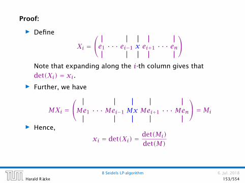
Proof:
ñ Define
Xi =e1 · · · ei−1 x ei+1 · · · en
Note that expanding along the i-th column gives that
det(Xi) = xi.ñ Further, we have
MXi =Me1 · · · Mei−1 Mx Mei+1 · · · Men
= Mi
ñ Hence,
xi = det(Xi) = det(Mi)det(M)
8 Seidels LP-algorithm 6. Jul. 2018
Harald Räcke 153/554

Bounding the Determinant
Let Z be the maximum absolute entry occuring in A, b or c. Let
C denote the matrix obtained from AB by replacing the j-thcolumn with vector b (for some j).
Observe that
|det(C)| =∣∣∣∣∣∣∑
π∈Smsgn(π)
∏
1≤i≤mCiπ(i)
∣∣∣∣∣∣
≤∑
π∈Sm
∏
1≤i≤m|Ciπ(i)|
≤m! · Zm . Here sgn(π) denotes the sign of the permu-tation, which is 1 if the permutation can begenerated by an even number of transposi-tions (exchanging two elements), and −1 ifthe number of transpositions is odd.The first identity is known as Leibniz formula.
8 Seidels LP-algorithm 6. Jul. 2018
Harald Räcke 154/554

Bounding the Determinant
Alternatively, Hadamards inequality gives
|det(C)| ≤m∏
i=1
‖C∗i‖ ≤m∏
i=1
(√mZ)
≤mm/2Zm .
8 Seidels LP-algorithm 6. Jul. 2018
Harald Räcke 155/554

Hadamards Inequality
e1
e2
e3
a1
a2
a3
|det(a1 a2 a3
)|
Hadamards inequality says that the volume of the red
parallelepiped (Spat) is smaller than the volume in the black
cube (if ‖e1‖ = ‖a1‖, ‖e2‖ = ‖a2‖, ‖e3‖ = ‖a3‖).
8 Seidels LP-algorithm 6. Jul. 2018
Harald Räcke 156/554

Ensuring Conditions
Given a standard minimization LP
min cTxs.t. Ax ≥ b
x ≥ 0
how can we obtain an LP of the required form?
ñ Compute a lower bound on cTx for any basic feasible
solution. Add the constraint cTx ≥ −dZ(m! ·Zm)− 1. Note
that this constraint is superfluous unless the LP is
unbounded.

Ensuring Conditions
Compute an optimum basis for the new LP.
ñ If the cost is cTx = −(dZ)(m! · Zm)− 1 we know that the
original LP is unbounded.
ñ Otw. we have an optimum basis.
8 Seidels LP-algorithm 6. Jul. 2018
Harald Räcke 158/554

In the following we use H to denote the set of all constraints
apart from the constraint cTx ≥ −dZ(m! · Zm)− 1.
We give a routine SeidelLP(H , d) that is given a set H of
explicit, non-degenerate constraints over d variables, and
minimizes cTx over all feasible points.
In addition it obeys the implicit constraint
cTx ≥ −(dZ)(m! · Zm)− 1.
8 Seidels LP-algorithm 6. Jul. 2018
Harald Räcke 159/554

Algorithm 1 SeidelLP(H , d)1: if d = 1 then solve 1-dimensional problem and return;
2: if H = then return x on implicit constraint hyperplane
3: choose random constraint h ∈H4: H ←H \ h5: x∗ ← SeidelLP(H , d)6: if x∗ = infeasible then return infeasible
7: if x∗ fulfills h then return x∗
8: // optimal solution fulfills h with equality, i.e., aThx = bh9: solve aThx = bh for some variable x`;
10: eliminate x` in constraints from H and in implicit constr.;
11: x∗ ← SeidelLP(H , d− 1)12: if x∗ = infeasible then
13: return infeasible
14: else
15: add the value of x` to x∗ and return the solution

8 Seidels LP-algorithm
ñ If d = 1 we can solve the 1-dimensional problem in time
O(maxm,1).ñ If d > 1 and m = 0 we take time O(d) to return
d-dimensional vector x.
ñ The first recursive call takes time T(m− 1, d) for the call
plus O(d) for checking whether the solution fulfills h.
ñ If we are unlucky and x∗ does not fulfill h we need time
O(d(m+ 1)) = O(dm) to eliminate x`. Then we make a
recursive call that takes time T(m− 1, d− 1).ñ The probability of being unlucky is at most d/m as there
are at most d constraints whose removal will decrease the
objective function
Note that for the case d = 1, the asymp-totic bound O(maxm,1) is valid alsofor the case m = 0.
8 Seidels LP-algorithm 6. Jul. 2018
Harald Räcke 161/554

8 Seidels LP-algorithm
This gives the recurrence
T(m,d) =
O(max1,m) if d = 1O(d) if d > 1 and m = 0O(d)+ T(m− 1, d)+dm (O(dm)+ T(m− 1, d− 1)) otw.
Note that T(m,d) denotes the expected running time.
8 Seidels LP-algorithm 6. Jul. 2018
Harald Räcke 162/554

8 Seidels LP-algorithm
Let C be the largest constant in the O-notations.
T(m,d) =
Cmax1,m if d = 1Cd if d > 1 and m = 0Cd+ T(m− 1, d)+dm (Cdm+ T(m− 1, d− 1)) otw.
Note that T(m,d) denotes the expected running time.
8 Seidels LP-algorithm 6. Jul. 2018
Harald Räcke 163/554

8 Seidels LP-algorithm
Let C be the largest constant in the O-notations.
We show T(m,d) ≤ Cf(d)max1,m.
d = 1:
T(m,1) ≤ Cmax1,m≤Cf(1)max1,m for f(1) ≥ 1
d > 1;m = 0 :
T(0, d) ≤ O(d) ≤ Cd≤Cf(d)max1,m for f(d) ≥ d
d > 1;m = 1 :
T(1, d) = O(d)+ T(0, d)+ d(O(d)+ T(0, d− 1)
)
≤ Cd+ Cd+ Cd2 + dCf(d− 1)
≤ Cf(d)max1,m for f(d) ≥ 3d2 + df(d− 1)

8 Seidels LP-algorithm
d > 1;m > 1 :
(by induction hypothesis statm. true for d′ < d,m′ ≥ 0;
and for d′ = d, m′ <m)
T(m,d) = O(d)+ T(m− 1, d)+ dm
(O(dm)+ T(m− 1, d− 1)
)
≤ Cd+ Cf(d)(m− 1)+ Cd2 + dmCf(d− 1)(m− 1)
≤ 2Cd2 + Cf(d)(m− 1)+ dCf(d− 1)
≤ Cf(d)m
if f(d) ≥ df(d− 1)+ 2d2.
8 Seidels LP-algorithm 6. Jul. 2018
Harald Räcke 165/554

8 Seidels LP-algorithm
ñ Define f(1) = 3 · 12 and f(d) = df(d− 1)+ 3d2 for d > 1.
Then
f(d) = 3d2 + df(d− 1)
= 3d2 + d[3(d− 1)2 + (d− 1)f (d− 2)
]
= 3d2 + d[3(d− 1)2 + (d− 1)
[3(d− 2)2 + (d− 2)f (d− 3)
]]
= 3d2 + 3d(d− 1)2 + 3d(d− 1)(d− 2)2 + . . .+ 3d(d− 1)(d− 2) · . . . · 4 · 3 · 2 · 12
= 3d!
(d2
d!+ (d− 1)2
(d− 1)!+ (d− 2)2
(d− 2)!+ . . .
)
= O(d!)
since∑i≥1
i2i! is a constant. ∑
i≥1
i2
i!=∑
i≥0
i+ 1i!
= e+∑
i≥1
ii!= 2e
8 Seidels LP-algorithm 6. Jul. 2018
Harald Räcke 166/554

Complexity
LP Feasibility Problem (LP feasibility A)
Given A ∈ Zm×n, b ∈ Zm. Does there exist x ∈ Rn with Ax ≤ b,
x ≥ 0?
LP Feasiblity Problem (LP feasibility B)
Given A ∈ Zm×n, b ∈ Zm. Find x ∈ Rn with Ax ≤ b, x ≥ 0!
LP Optimization A
Given A ∈ Zm×n, b ∈ Zm, c ∈ Zn. What is the maximum value of
cTx for a feasible point x ∈ Rn?
LP Optimization B
Given A ∈ Zm×n, b ∈ Zm, c ∈ Zn. Return feasible point x ∈ Rn
with maximum value of cTx?
Note that allowing A,b to contain rational numbers does not make a difference, as we canmultiply every number by a suitable large constant so that everything becomes integral but thefeasible region does not change.

The Bit Model
Input size
ñ The number of bits to represent a number a ∈ Z is
dlog2(|a|)e + 1
ñ Let for an m×n matrix M, L(M) denote the number of bits
required to encode all the numbers in M.
〈M〉 :=∑
i,jdlog2(|mij|)+ 1e
ñ In the following we assume that input matrices are encoded
in a standard way, where each number is encoded in binary
and then suitable separators are added in order to separate
distinct number from each other.
ñ Then the input length is L = Θ(〈A〉 + 〈b〉).

ñ In the following we sometimes refer to L := 〈A〉 + 〈b〉 as the
input size (even though the real input size is something in
Θ(〈A〉 + 〈b〉)).ñ Sometimes we may also refer to L := 〈A〉 + 〈b〉 +n log2n as
the input size. Note that n log2n = Θ(〈A〉 + 〈b〉).ñ In order to show that LP-decision is in NP we show that if
there is a solution x then there exists a small solution for
which feasibility can be verified in polynomial time
(polynomial in L).
Note that m log2m may be much largerthan 〈A〉 + 〈b〉.
9 The Ellipsoid Algorithm 6. Jul. 2018
Harald Räcke 169/554

Suppose that Ax = b; x ≥ 0 is feasible.
Then there exists a basic feasible solution. This means a set B of
basic variables such that
xB = A−1B b
and all other entries in x are 0.
In the following we show that this x has small encoding lengthand we give an explicit bound on this length. So far we haveonly been handwaving and have said that we can compute x viaGaussian elimination and it will be short...
9 The Ellipsoid Algorithm 6. Jul. 2018
Harald Räcke 170/554

Size of a Basic Feasible Solution
ñ A: original input matrix
ñ A: transformation of A into standard form
ñ AB: submatrix of A corresponding to basis B
Lemma 47
Let AB ∈ Zm×m and b ∈ Zm. Define L = 〈A〉 + 〈b〉 +n log2n.
Then a solution to ABxB = b has rational components xj of the
formDjD , where |Dj| ≤ 2L and |D| ≤ 2L.
Proof:
Cramers rules says that we can compute xj as
xj =det(AjB)det(AB)
where AjB is the matrix obtained from AB by replacing the j-thcolumn by the vector b.
Note that n in the theorem denotesthe number of columns in A whichmay be much smaller than m.

Bounding the Determinant
Let X = AB. Then
|det(X)| = |det(X)|
=∣∣∣∣∣∣∑
π∈Snsgn(π)
∏
1≤i≤nXiπ(i)
∣∣∣∣∣∣
≤∑
π∈Sn
∏
1≤i≤n|Xiπ(i)|
≤ n! · 2〈A〉+〈b〉 ≤ 2L .
Here X is an n× n submatrix of Awith n ≤ n.
Analogously for det(AjB).
When computing the determinant of X = ABwe first do expansions along columns thatwere introduced when transforming A intostandard form, i.e., into A.
Such a column contains a single 1 andthe remaining entries of the column are 0.Therefore, these expansions do not increasethe absolute value of the determinant. Afterwe did expansions for all these columns weare left with a square sub-matrix of A of sizeat most n×n.
9 The Ellipsoid Algorithm 6. Jul. 2018
Harald Räcke 172/554

Reducing LP-solving to LP decision.
Given an LP maxcTx | Ax ≤ b;x ≥ 0 do a binary search for the
optimum solution
(Add constraint cTx ≥ M). Then checking for feasibility shows
whether optimum solution is larger or smaller than M).
If the LP is feasible then the binary search finishes in at most
log2
(2n22L′
1/2L′)= O(L′) ,
as the range of the search is at most −n22L′ , . . . , n22L′ and the
distance between two adjacent values is at least 1det(A) ≥ 1
2L′ .
Here we use L′ = 〈A〉 + 〈b〉 + 〈c〉 +n log2n (it also includes the
encoding size of c).

How do we detect whether the LP is unbounded?
Let Mmax = n22L′ be an upper bound on the objective value of a
basic feasible solution.
We can add a constraint cTx ≥ Mmax+1 and check for feasibility.
9 The Ellipsoid Algorithm 6. Jul. 2018
Harald Räcke 174/554

Ellipsoid Methodñ Let K be a convex set.
ñ Maintain ellipsoid E that is guaranteed tocontain K provided that K is non-empty.
ñ If center z ∈ K STOP.
ñ Otw. find a hyperplane separatingK from z (e.g. a violatedconstraint in the LP).
ñ Shift hyperplane to containnode z. H denotes half-space that contains K.
ñ Compute (smallest)ellipsoid E′ thatcontains E ∩H.
ñ REPEAT
K
z
E
z′
9 The Ellipsoid Algorithm 6. Jul. 2018
Harald Räcke 175/554

Issues/Questions:
ñ How do you choose the first Ellipsoid? What is its volume?
ñ How do you measure progress? By how much does the
volume decrease in each iteration?
ñ When can you stop? What is the minimum volume of a
non-empty polytop?
9 The Ellipsoid Algorithm 6. Jul. 2018
Harald Räcke 176/554

Definition 48
A mapping f : Rn → Rn with f(x) = Lx + t, where L is an
invertible matrix is called an affine transformation.
9 The Ellipsoid Algorithm 6. Jul. 2018
Harald Räcke 177/554

Definition 49
A ball in Rn with center c and radius r is given by
B(c, r) = x | (x − c)T (x − c) ≤ r2= x |
∑
i(x − c)2i /r2 ≤ 1
B(0,1) is called the unit ball.
9 The Ellipsoid Algorithm 6. Jul. 2018
Harald Räcke 178/554

Definition 50
An affine transformation of the unit ball is called an ellipsoid.
From f(x) = Lx + t follows x = L−1(f (x)− t).
f(B(0,1)) = f(x) | x ∈ B(0,1)= y ∈ Rn | L−1(y − t) ∈ B(0,1)= y ∈ Rn | (y − t)TL−1TL−1(y − t) ≤ 1= y ∈ Rn | (y − t)TQ−1(y − t) ≤ 1
where Q = LLT is an invertible matrix.
9 The Ellipsoid Algorithm 6. Jul. 2018
Harald Räcke 179/554

How to Compute the New Ellipsoid
ñ Use f−1 (recall that f = Lx + t is the affine transformationof the unit ball) to rotate/distort the ellipsoid (back) into theunit ball.
ñ Use a rotation R−1 to rotate the unit ball such that thenormal vector of the halfspace is parallel to e1.
ñ Compute the new center c′ andthe new matrix Q′ for thissimplified setting.
ñ Use the transformationsR and f to get thenew center c′ andthe new matrix Q′
for the originalellipsoid E.
ccc
E EE
a
c ′c′c′
E′ E′E′aa
9 The Ellipsoid Algorithm 6. Jul. 2018
Harald Räcke 180/554

The Easy Case
E′
e1
e2
c′
ñ The new center lies on axis x1. Hence, c′ = te1 for t > 0.
ñ The vectors e1, e2, . . . have to fulfill the ellipsoid constraint
with equality. Hence (ei − c′)T Q′−1(ei − c′) = 1.
9 The Ellipsoid Algorithm 6. Jul. 2018
Harald Räcke 181/554

The Easy Case
ñ To obtain the matrix Q′−1
for our ellipsoid E′ note that E′ is
axis-parallel.
ñ Let a denote the radius along the x1-axis and let b denote
the (common) radius for the other axes.
ñ The matrix
L′ =
a 0 . . . 0
0 b. . .
......
. . .. . . 0
0 . . . 0 b
maps the unit ball (via function f ′(x) = L′x) to an
axis-parallel ellipsoid with radius a in direction x1 and b in
all other directions.
9 The Ellipsoid Algorithm 6. Jul. 2018
Harald Räcke 182/554

The Easy Case
ñ As Q′ = L′L′t the matrix Q′−1
is of the form
Q′−1 =
1a2 0 . . . 0
0 1b2
. . ....
.... . .
. . . 0
0 . . . 0 1b2
9 The Ellipsoid Algorithm 6. Jul. 2018
Harald Räcke 183/554

The Easy Case
ñ (e1 − c′)T Q′−1(e1 − c′) = 1 gives
1− t0...
0
T
·
1a2 0 . . . 0
0 1b2
. . ....
.... . .
. . . 0
0 . . . 0 1b2
·
1− t0...
0
= 1
ñ This gives (1− t)2 = a2.
9 The Ellipsoid Algorithm 6. Jul. 2018
Harald Räcke 184/554

The Easy Case
ñ For i ≠ 1 the equation (ei − c′)T Q′−1(ei − c′) = 1 looks like
(here i = 2)
−t1
0...
0
T
·
1a2 0 . . . 0
0 1b2
. . ....
.... . .
. . . 0
0 . . . 0 1b2
·
−t1
0...
0
= 1
ñ This gives t2a2 + 1
b2 = 1, and hence
1b2 = 1− t
2
a2 = 1− t2
(1− t)2 =1− 2t(1− t)2
9 The Ellipsoid Algorithm 6. Jul. 2018
Harald Räcke 185/554

Summary
So far we have
a = 1− t and b = 1− t√1− 2t
9 The Ellipsoid Algorithm 6. Jul. 2018
Harald Räcke 186/554

The Easy Case
We still have many choices for t:
E
e1
e2
c′E′
Choose t such that the volume of E′ is minimal!!!
9 The Ellipsoid Algorithm 6. Jul. 2018
Harald Räcke 187/554

The Easy Case
We want to choose t such that the volume of E′ is minimal.
Lemma 51
Let L be an affine transformation and K ⊆ Rn. Then
vol(L(K)) = |det(L)| · vol(K) .
9 The Ellipsoid Algorithm 6. Jul. 2018
Harald Räcke 188/554

n-dimensional volume
e1
e2
e3
a1
a2
a3
|det(a1 a2 a3
)|
9 The Ellipsoid Algorithm 6. Jul. 2018
Harald Räcke 189/554

The Easy Case
ñ We want to choose t such that the volume of E′ is minimal.
vol(E′) = vol(B(0,1)) · |det(L′)| ,
ñ Recall that
L′ =
a 0 . . . 0
0 b. . .
......
. . .. . . 0
0 . . . 0 b
ñ Note that a and b in the above equations depend on t, by
the previous equations.
9 The Ellipsoid Algorithm 6. Jul. 2018
Harald Räcke 190/554

The Easy Case
vol(E′) = vol(B(0,1)) · |det(L′)|= vol(B(0,1)) · abn−1
= vol(B(0,1)) · (1− t) ·(
1− t√1− 2t
)n−1
= vol(B(0,1)) · (1− t)n(√
1− 2t)n−1
We use the shortcut Φ := vol(B(0,1)).
9 The Ellipsoid Algorithm 6. Jul. 2018
Harald Räcke 191/554

The Easy Case
d vol(E′)d t
= dd t
(Φ(1− t)n(√1−2t)n−1
)
= ΦN2 ·
((−1) ·n(1− t)n−1 · (
√1− 2t)n−1
−(n− 1)(√
1− 2t)n−2 · 1
2√
1− 2t· (−2) · (1− t)n
)
= ΦN2 · (
√1− 2t)n−3 · (1− t)n−1
·((n− 1)(1− t)−n(1− 2t)
)
= ΦN2 · (
√1− 2t)n−3 · (1− t)n−1 ·
((n+ 1)t − 1
)
NN = denominator
(−1) ·n(1− t)n−1
derivative of numerator
(1− t)n
(√
1− 2t)n−1
denominator
(√1−2t)n−1
(n− 1)(√
1− 2t)n−2
outer derivative
(√1−2t)n−1√1−2t
√1− 2t
1
2√
1− 2t· (−2)
inner derivative
√1−2t
(1− t)nnumerator
(1− t)n
1− 2t
1− t
9 The Ellipsoid Algorithm 6. Jul. 2018
Harald Räcke 192/554

The Easy Case
ñ We obtain the minimum for t = 1n+1 .
ñ For this value we obtain
a = 1− t = nn+ 1
and b = 1− t√1− 2t
= n√n2 − 1
To see the equation for b, observe that
b2 = (1− t)2
1− 2t= (1−
1n+1)
2
1− 2n+1
= (nn+1)
2
n−1n+1
= n2
n2 − 1
9 The Ellipsoid Algorithm 6. Jul. 2018
Harald Räcke 193/554
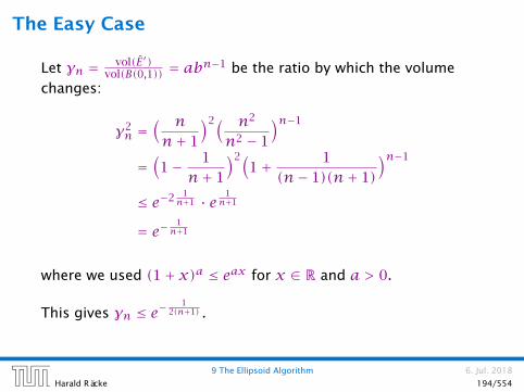
The Easy Case
Let γn = vol(E′)vol(B(0,1)) = abn−1 be the ratio by which the volume
changes:
γ2n =
( nn+ 1
)2( n2
n2 − 1
)n−1
=(1− 1
n+ 1
)2(1+ 1
(n− 1)(n+ 1)
)n−1
≤ e−2 1n+1 · e 1
n+1
= e− 1n+1
where we used (1+ x)a ≤ eax for x ∈ R and a > 0.
This gives γn ≤ e−1
2(n+1) .
9 The Ellipsoid Algorithm 6. Jul. 2018
Harald Räcke 194/554

How to Compute the New Ellipsoid
ñ Use f−1 (recall that f = Lx + t is the affine transformationof the unit ball) to translate/distort the ellipsoid (back) intothe unit ball.
ñ Use a rotation R−1 to rotate the unit ball such that thenormal vector of the halfspace is parallel to e1.
ñ Compute the new center c′ andthe new matrix Q′ for thissimplified setting.
ñ Use the transformationsR and f to get thenew center c′ andthe new matrix Q′
for the originalellipsoid E.
ccc
E EE
a
c ′c′c′
E′ E′E′aa
9 The Ellipsoid Algorithm 6. Jul. 2018
Harald Räcke 195/554

Our progress is the same:
e−1
2(n+1) ≥ vol(E′)vol(B(0,1))
= vol(E′)vol(E)
= vol(R(E′))vol(R(E))
= vol(E′)vol(E)
= vol(f (E′))vol(f (E))
= vol(E′)vol(E)
Here it is important that mapping a set with affine function
f(x) = Lx + t changes the volume by factor det(L).
9 The Ellipsoid Algorithm 6. Jul. 2018
Harald Räcke 196/554

The Ellipsoid Algorithm
How to compute the new parameters?
The transformation function of the (old) ellipsoid: f(x) = Lx+ c;
The halfspace to be intersected: H = x | aT (x − c) ≤ 0;
f−1(H) = f−1(x) | aT (x − c) ≤ 0= f−1(f (y)) | aT (f (y)− c) ≤ 0= y | aT (f (y)− c) ≤ 0= y | aT (Ly + c − c) ≤ 0= y | (aTL)y ≤ 0
This means a = LTa.The center c is of course at the origin.
9 The Ellipsoid Algorithm 6. Jul. 2018
Harald Räcke 197/554

The Ellipsoid Algorithm
After rotating back (applying R−1) the normal vector of the
halfspace points in negative x1-direction. Hence,
R−1( LTa‖LTa‖
)= −e1 ⇒ − LTa
‖LTa‖ = R · e1
Hence,
c′ = R · c′ = R · 1n+ 1
e1 = − 1n+ 1
LTa‖LTa‖
c′ = f(c′) = L · c′ + c
= − 1n+ 1
LLTa‖LTa‖ + c
= c − 1n+ 1
Qa√aTQa

For computing the matrix Q′ of the new ellipsoid we assume in
the following that E′, E′ and E′ refer to the ellispoids centered in
the origin.
9 The Ellipsoid Algorithm 6. Jul. 2018
Harald Räcke 199/554

Recall that
Q′ =
a2 0 . . . 0
0 b2 . . ....
.... . .
. . . 0
0 . . . 0 b2
This gives
Q′ = n2
n2 − 1
(I − 2
n+ 1e1eT1
)
because for a2 = n2/(n+1)2 and b2 = n2/n2−1
b2 − b2 2n+ 1
= n2
n2 − 1− 2n2
(n− 1)(n+ 1)2
= n2(n+ 1)− 2n2
(n− 1)(n+ 1)2= n2(n− 1)(n− 1)(n+ 1)2
= a2
Note that e1eT1 is a matrixM that has M11 = 1 and allother entries equal to 0.

9 The Ellipsoid Algorithm
E′ = R(E′)= R(x) | xT Q′−1
x ≤ 1= y | (R−1y)T Q′
−1R−1y ≤ 1
= y | yT (RT )−1Q′−1R−1y ≤ 1
= y | yT (RQ′RT︸ ︷︷ ︸Q′
)−1y ≤ 1
9 The Ellipsoid Algorithm 6. Jul. 2018
Harald Räcke 201/554

9 The Ellipsoid Algorithm
Hence,
Q′ = RQ′RT
= R · n2
n2 − 1
(I − 2
n+ 1e1eT1
)· RT
= n2
n2 − 1
(R · RT − 2
n+ 1(Re1)(Re1)T
)
= n2
n2 − 1
(I − 2
n+ 1LTaaTL‖LTa‖2
)
Here we used the equation for Re1 proved before, and the fact that RRT = I, which holds forany rotation matrix. To see this observe that the length of a rotated vector x should not change,i.e.,
xT Ix = (Rx)T (Rx) = xT (RTR)xwhich means xT (I−RTR)x = 0 for every vector x. It is easy to see that this can only be fulfilledif I − RTR = 0.
9 The Ellipsoid Algorithm 6. Jul. 2018
Harald Räcke 202/554

9 The Ellipsoid Algorithm
E′ = L(E′)= L(x) | xT Q′−1x ≤ 1= y | (L−1y)T Q′−1L−1y ≤ 1= y | yT (LT )−1Q′−1L−1y ≤ 1= y | yT (LQ′LT︸ ︷︷ ︸
Q′
)−1y ≤ 1
9 The Ellipsoid Algorithm 6. Jul. 2018
Harald Räcke 203/554

9 The Ellipsoid Algorithm
Hence,
Q′ = LQ′LT
= L · n2
n2 − 1
(I − 2
n+ 1LTaaTLaTQa
)· LT
= n2
n2 − 1
(Q− 2
n+ 1QaaTQaTQa
)
9 The Ellipsoid Algorithm 6. Jul. 2018
Harald Räcke 204/554

Incomplete Algorithm
Algorithm 1 ellipsoid-algorithm
1: input: point c ∈ Rn, convex set K ⊆ Rn
2: output: point x ∈ K or “K is empty”
3: Q ← ???
4: repeat
5: if c ∈ K then return c6: else
7: choose a violated hyperplane a
8: c ← c − 1n+ 1
Qa√aTQa
9: Q ← n2
n2 − 1
(Q− 2
n+ 1QaaTQaTQa
)
10: endif
11: until ???
12: return “K is empty”
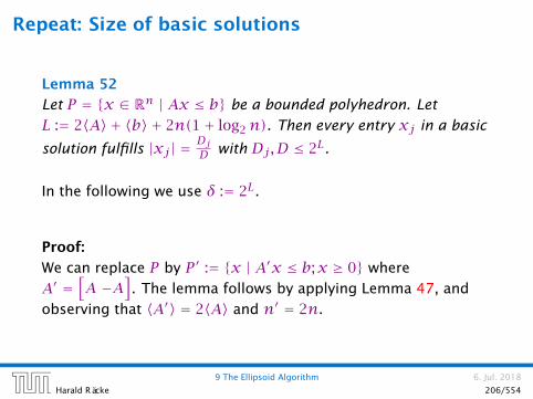
Repeat: Size of basic solutions
Lemma 52
Let P = x ∈ Rn | Ax ≤ b be a bounded polyhedron. Let
L := 2〈A〉 + 〈b〉 + 2n(1+ log2n). Then every entry xj in a basic
solution fulfills |xj| = DjD with Dj ,D ≤ 2L.
In the following we use δ := 2L.
Proof:
We can replace P by P ′ := x | A′x ≤ b;x ≥ 0 where
A′ =[A −A
]. The lemma follows by applying Lemma 47, and
observing that 〈A′〉 = 2〈A〉 and n′ = 2n.
9 The Ellipsoid Algorithm 6. Jul. 2018
Harald Räcke 206/554

How do we find the first ellipsoid?
For feasibility checking we can assume that the polytop P is
bounded; it is sufficient to consider basic solutions.
Every entry xi in a basic solution fulfills |xi| ≤ δ.
Hence, P is contained in the cube −δ ≤ xi ≤ δ.
A vector in this cube has at most distance R := √nδ from the
origin.
Starting with the ball E0 := B(0, R) ensures that P is completely
contained in the initial ellipsoid. This ellipsoid has volume at
most Rn vol(B(0,1)) ≤ (nδ)n vol(B(0,1)).
9 The Ellipsoid Algorithm 6. Jul. 2018
Harald Räcke 207/554

When can we terminate?
Let P := x | Ax ≤ b with A ∈ Z and b ∈ Z be a bounded
polytop.
Consider the following polyhedron
Pλ :=x | Ax ≤ b + 1
λ
1...
1
,
where λ = δ2 + 1.
Note that the volume of Pλ cannot be 0
9 The Ellipsoid Algorithm 6. Jul. 2018
Harald Räcke 208/554

Making P full-dimensional
Lemma 53
Pλ is feasible if and only if P is feasible.
⇐= : obvious!
9 The Ellipsoid Algorithm 6. Jul. 2018
Harald Räcke 209/554

Making P full-dimensional
=⇒:
Consider the polyhedrons
P =x |
[A −A Im
]x = b;x ≥ 0
and
Pλ =x |
[A −A Im
]x = b + 1
λ
1...
1
;x ≥ 0
.
P is feasible if and only if P is feasible, and Pλ feasible if and
only if Pλ feasible.
Pλ is bounded since Pλ and P are bounded.

Making P full-dimensional
Let A =[A −A Im
].
Pλ feasible implies that there is a basic feasible solution
represented by
xB = A−1B b +
1λA−1B
1...
1
(The other x-values are zero)
The only reason that this basic feasible solution is not feasible
for P is that one of the basic variables becomes negative.
Hence, there exists i with
(A−1B b)i < 0 ≤ (A−1
B b)i +1λ(A−1B ~1)i

Making P full-dimensional
By Cramers rule we get
(A−1B b)i < 0 =⇒ (A−1
B b)i ≤ −1
det(AB)≤ −1/δ
and
(A−1B ~1)i ≤ det(AjB) ≤ δ ,
where AjB is obtained by replacing the j-th column of AB by ~1.
But then
(A−1B b)i +
1λ(A−1B ~1)i ≤ −1/δ+ δ/λ < 0 ,
as we chose λ = δ2 + 1. Contradiction.
9 The Ellipsoid Algorithm 6. Jul. 2018
Harald Räcke 212/554

Lemma 54
If Pλ is feasible then it contains a ball of radius r := 1/δ3. This
has a volume of at least rnvol(B(0,1)) = 1δ3n vol(B(0,1)).
Proof:
If Pλ feasible then also P . Let x be feasible for P .
This means Ax ≤ b.
Let ~with ‖ ~‖ ≤ r . Then
(A(x + ~))i = (Ax)i + (A~)i ≤ bi + ~aTi ~
≤ bi + ‖~ai‖ · ‖ ~‖ ≤ bi +√n · 2〈amax〉 · r
≤ bi +√n · 2〈amax〉
δ3 ≤ bi + 1δ2 + 1
≤ bi + 1λ
Hence, x + ~ is feasible for Pλ which proves the lemma.
9 The Ellipsoid Algorithm 6. Jul. 2018
Harald Räcke 213/554

How many iterations do we need until the volume becomes too
small?
e−i
2(n+1) · vol(B(0, R)) < vol(B(0, r ))
Hence,
i > 2(n+ 1) ln(vol(B(0, R))
vol(B(0, r ))
)
= 2(n+ 1) ln(nnδn · δ3n
)
= 8n(n+ 1) ln(δ)+ 2(n+ 1)n ln(n)
= O(poly(n) · L)
9 The Ellipsoid Algorithm 6. Jul. 2018
Harald Räcke 214/554

Algorithm 1 ellipsoid-algorithm
1: input: point c ∈ Rn, convex set K ⊆ Rn, radii R and r2: with K ⊆ B(c,R), and B(x, r) ⊆ K for some x3: output: point x ∈ K or “K is empty”
4: Q ← diag(R2, . . . , R2) // i.e., L = diag(R, . . . , R)5: repeat
6: if c ∈ K then return c7: else
8: choose a violated hyperplane a
9: c ← c − 1n+ 1
Qa√aTQa
10: Q ← n2
n2 − 1
(Q− 2
n+ 1QaaTQaTQa
)
11: endif
12: until det(Q) ≤ r2n // i.e., det(L) ≤ rn13: return “K is empty”

Separation Oracle
Let K ⊆ Rn be a convex set. A separation oracle for K is an
algorithm A that gets as input a point x ∈ Rn and either
ñ certifies that x ∈ K,
ñ or finds a hyperplane separating x from K.
We will usually assume that A is a polynomial-time algorithm.
In order to find a point in K we need
ñ a guarantee that a ball of radius r is contained in K,
ñ an initial ball B(c,R) with radius R that contains K,
ñ a separation oracle for K.
The Ellipsoid algorithm requires O(poly(n) · log(R/r))iterations. Each iteration is polytime for a polynomial-time
Separation oracle.

Example
9 The Ellipsoid Algorithm 6. Jul. 2018
Harald Räcke 217/554

10 Karmarkars Algorithm
ñ inequalities Ax ≤ b; m×n matrix A with rows aTiñ P = x | Ax ≤ b; P := x | Ax < bñ interior point algorithm: x ∈ P throughout the algorithm
ñ for x ∈ P define
si(x) := bi − aTi xas the slack of the i-th constraint
logarithmic barrier function:
φ(x) = −m∑
i=1
ln(si(x))
Penalty for point x; points close to the boundary have a very
large penalty.Throughout this section ai denotes thei-th row as a column vector.

Penalty Function
−2 −1 0 1 2 3 4 5
−2
−1
0
1
2
−2
0
2
4
6
8
10
10 Karmarkars Algorithm 6. Jul. 2018
Harald Räcke 219/554

Penalty Function
−2 0 2 4 −2
02
0
5
10
−2
0
2
4
6
8
10
10 Karmarkars Algorithm 6. Jul. 2018
Harald Räcke 220/554

Gradient and Hessian
Taylor approximation:
φ(x + ε) ≈ φ(x)+∇φ(x)Tε+ 12εT∇2φ(x)ε
Gradient:
∇φ(x) =m∑
i=1
1si(x)
· ai = ATdx
where dTx = (1/s1(x), . . . ,1/sm(x)). (dx vector of inverse slacks)
Hessian:
Hx := ∇2φ(x) =m∑
i=1
1si(x)2
aiaTi = ATD2xA
with Dx = diag(dx).

Proof for Gradient
∂φ(x)∂xi
= ∂∂xi
(−∑r
ln(sr (x)))
= −∑r
∂∂xi
(ln(sr (x))
)= −
∑r
1sr (x)
∂∂xi
(sr (x)
)
= −∑r
1sr (x)
∂∂xi
(br − aTr x
)=∑r
1sr (x)
∂∂xi
(aTr x
)
=∑r
1sr (x)
Ari
The i-th entry of the gradient vector is∑r 1/sr (x) ·Ari. This
gives that the gradient is
∇φ(x) =∑r
1/sr (x)ar = ATdx

Proof for Hessian
∂∂xj
(∑r
1sr (x)
Ari)=∑rAri
(− 1sr (x)2
)· ∂∂xj
(sr (x)
)
=∑rAri
1sr (x)2
Arj
Note that∑r AriArj = (ATA)ij. Adding the additional factors
1/sr (x)2 can be done with a diagonal matrix.
Hence the Hessian is
Hx = ATD2A

Properties of the Hessian
Hx is positive semi-definite for x ∈ P
uTHxu = uTATD2xAu = ‖DxAu‖2
2 ≥ 0
This gives that φ(x) is convex.
If rank(A) = n, Hx is positive definite for x ∈ P
uTHxu = ‖DxAu‖22 > 0 for u ≠ 0
This gives that φ(x) is strictly convex.
‖u‖Hx := √uTHxu is a (semi-)norm; the unit ball w.r.t. this norm
is an ellipsoid.
10 Karmarkars Algorithm 6. Jul. 2018
Harald Räcke 224/554

Dikin Ellipsoid
Ex = y | (y − x)THx(y − x) ≤ 1 = y | ‖y − x‖Hx ≤ 1
Points in Ex are feasible!!!
(y − x)THx(y − x) = (y − x)TATD2xA(y − x)
=m∑
i=1
(aTi (y − x))2si(x)2
=m∑
i=1
(change of distance to i-th constraint going from x to y)2
(distance of x to i-th constraint)2
≤ 1
In order to become infeasible when going from x to y one of the
terms in the sum would need to be larger than 1.

Dikin Ellipsoids
10 Karmarkars Algorithm 6. Jul. 2018
Harald Räcke 226/554
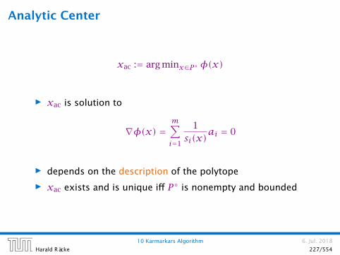
Analytic Center
xac := arg minx∈P φ(x)
ñ xac is solution to
∇φ(x) =m∑
i=1
1si(x)
ai = 0
ñ depends on the description of the polytope
ñ xac exists and is unique iff P is nonempty and bounded
10 Karmarkars Algorithm 6. Jul. 2018
Harald Räcke 227/554

Central Path
In the following we assume that the LP and its dual are strictly
feasible and that rank(A) = n.
Central Path:
Set of points x∗(t) | t > 0 with
x∗(t) = argminxtcTx +φ(x)
ñ t = 0: analytic center
ñ t = ∞: optimum solution
x∗(t) exists and is unique for all t ≥ 0.
10 Karmarkars Algorithm 6. Jul. 2018
Harald Räcke 228/554

Different Central Paths
x
y
10 Karmarkars Algorithm 6. Jul. 2018
Harald Räcke 229/554
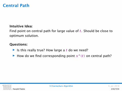
Central Path
Intuitive Idea:
Find point on central path for large value of t. Should be close to
optimum solution.
Questions:
ñ Is this really true? How large a t do we need?
ñ How do we find corresponding point x∗(t) on central path?
10 Karmarkars Algorithm 6. Jul. 2018
Harald Räcke 230/554

The Dual
primal-dual pair:
min cTx
s.t. Ax ≤ b
max −bTzs.t. ATz + c = 0
z ≥ 0
Assumptions
ñ primal and dual problems are strictly feasible;
ñ rank(A) = n.
Note that the right LP in standard formis equal to max−bTy | −ATy = c,x ≥0. The dual of this is mincTx | −Ax ≥−b (variables x are unrestricted).

Force Field Interpretation
Point x∗(t) on central path is solution to tc +∇φ(x) = 0
ñ We can view each constraint as generating a repelling force.
The combination of these forces is represented by ∇φ(x).ñ In addition there is a force tc pulling us towards the
optimum solution.
10 Karmarkars Algorithm 6. Jul. 2018
Harald Räcke 232/554
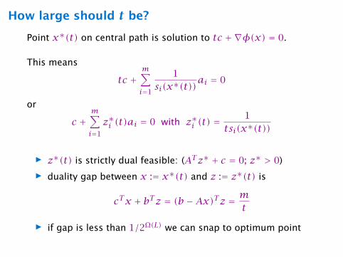
How large should t be?
Point x∗(t) on central path is solution to tc +∇φ(x) = 0.
This means
tc +m∑
i=1
1si(x∗(t))
ai = 0
or
c +m∑
i=1
z∗i (t)ai = 0 with z∗i (t) =1
tsi(x∗(t))
ñ z∗(t) is strictly dual feasible: (ATz∗ + c = 0; z∗ > 0)
ñ duality gap between x := x∗(t) and z := z∗(t) is
cTx + bTz = (b −Ax)Tz = mt
ñ if gap is less than 1/2Ω(L) we can snap to optimum point

How to find x∗(t)
First idea:
ñ start somewhere in the polytope
ñ use iterative method (Newtons method) to minimize
ft(x) := tcTx +φ(x)
10 Karmarkars Algorithm 6. Jul. 2018
Harald Räcke 234/554

Newton Method
Quadratic approximation of ft
ft(x + ε) ≈ ft(x)+∇ft(x)Tε+ 12εTHft(x) ε
Suppose this were exact:
ft(x + ε) = ft(x)+∇ft(x)Tε+ 12εTHft(x) ε
Then gradient is given by:
∇ft(x + ε) = ∇ft(x)+Hft(x) · εNote that for the one-dimensional caseg(ε) = f(x)+f ′(x)ε+ 1
2f′′(x)ε2, then
g′(ε) = f ′(x)+ f ′′(x)ε.
10 Karmarkars Algorithm 6. Jul. 2018
Harald Räcke 235/554

Newton Method
We want to move to a point where this gradient is 0:
Newton Step at x ∈ P
∆xnt = −H−1ft (x)∇ft(x)
= −H−1ft (x)(tc +∇φ(x))
= −(ATD2xA)−1(tc +ATdx)
Newton Iteration:
x := x +∆xnt
Observe that Hft (x) = H(x), where H(x) is the Hessianfor the function φ(x) (adding a linear term like tcTxdoes not affect the Hessian).
Also ∇ft(x) = tc +∇φ(x).

Measuring Progress of Newton Step
Newton decrement:
λt(x) = ‖DxA∆xnt‖= ‖∆xnt‖Hx
Square of Newton decrement is linear estimate of reduction if we
do a Newton step:
−λt(x)2 = ∇ft(x)T∆xnt
ñ λt(x) = 0 iff x = x∗(t)ñ λt(x) is measure of proximity of x to x∗(t)
Recall that ∆xnt fulfills −H(x)∆xnt = ∇ft().

Convergence of Newtons Method
Theorem 55
If λt(x) < 1 then
ñ x+ := x +∆xnt ∈ P (new point feasible)
ñ λt(x+) ≤ λt(x)2
This means we have quadratic convergence. Very fast.

Convergence of Newtons Method
feasibility:
ñ λt(x) = ‖∆xnt‖Hx < 1; hence x+ lies in the Dikin ellipsoid
around x.
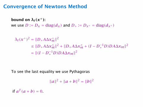
Convergence of Newtons Method
bound on λt(x+):we use D := Dx = diag(dx) and D+ := Dx+ = diag(dx+)
λt(x+)2 = ‖D+A∆x+nt‖2
≤ ‖D+A∆x+nt‖2 + ‖D+A∆x+nt + (I −D−1+ D)DA∆xnt‖2
= ‖(I −D−1+ D)DA∆xnt‖2
To see the last equality we use Pythagoras
‖a‖2 + ‖a+ b‖2 = ‖b‖2
if aT (a+ b) = 0.
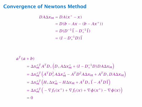
Convergence of Newtons Method
DA∆xnt = DA(x+ − x)= D(b −Ax − (b −Ax+))= D(D−1~1−D−1+ ~1)
= (I −D−1+ D)~1
aT (a+ b)= ∆x+Tnt ATD+
(D+A∆x+nt + (I −D−1+ D)DA∆xnt
)
= ∆x+Tnt
(ATD2+A∆x+nt −ATD2A∆xnt +ATD+DA∆xnt
)
= ∆x+Tnt
(H+∆x+nt −H∆xnt +ATD+~1−ATD~1
)
= ∆x+Tnt
(−∇ft(x+)+∇ft(x)+∇φ(x+)−∇φ(x)
)
= 0

Convergence of Newtons Method
bound on λt(x+):we use D := Dx = diag(dx) and D+ := Dx+ = diag(dx+)
λt(x+)2 = ‖D+A∆x+nt‖2
≤ ‖D+A∆x+nt‖2 + ‖D+A∆x+nt + (I −D−1+ D)DA∆xnt‖2
= ‖(I −D−1+ D)DA∆xnt‖2
= ‖(I −D−1+ D)2~1‖2
≤ ‖(I −D−1+ D)~1‖4
= ‖DA∆xnt‖4
= λt(x)4
The second inequality follows from∑iy4i ≤
(∑iy2i)2

If λt(x) is large we do not have a guarantee.
Try to avoid this case!!!
10 Karmarkars Algorithm 6. Jul. 2018
Harald Räcke 243/554

Path-following Methods
Try to slowly travel along the central path.
Algorithm 1 PathFollowing1: start at analytic center
2: while solution not good enough do
3: make step to improve objective function
4: recenter to return to central path

Short Step Barrier Method
simplifying assumptions:
ñ a first central point x∗(t0) is given
ñ x∗(t) is computed exactly in each iteration
ε is approximation we are aiming for
start at t = t0, repeat until m/t ≤ εñ compute x∗(µt) using Newton starting from x∗(t)ñ t := µt
where µ = 1+ 1/(2√m)

Short Step Barrier Method
gradient of ft+ at (x = x∗(t))
∇ft+(x) = ∇ft(x)+ (µ − 1)tc
= −(µ − 1)ATDx~1
This holds because 0 = ∇ft(x) = tc +ATDx~1.
The Newton decrement is
λt+(x)2 = ∇ft+(x)TH−1∇ft+(x)= (µ − 1)2~1TB(BTB)−1BT~1 B = DTxA≤ (µ − 1)2m
= 1/4
This means we are in the range of quadratic convergence!!!

Number of Iterations
the number of Newton iterations per outer
iteration is very small; in practise only 1 or 2
Number of outer iterations:
We need tk = µkt0 ≥m/ε. This holds when
k ≥ log(m/(εt0))log(µ)
We get a bound of
O(√m log
mεt0
)
We show how to get a starting point with t0 = 1/2L. Together
with ε ≈ 2−L we get O(L√m) iterations.
Explanation for previous slideP = B(BTB)−1BT is a symmet-ric real-valued matrix; it has nlinearly independent Eigenvec-tors. Since it is a projection ma-trix (P2 = P ) it can only haveEigenvalues 0 and 1 (becausethe Eigenvalues of P2 are λ2
i ,where λi is Eigenvalue of P ).The expression
maxvvTPvvTv
gives the largest Eigenvalue forP . Hence, ~1TP~1 ≤ ~1T~1 =m
10 Karmarkars Algorithm 6. Jul. 2018
Harald Räcke 247/554

Damped Newton Method
For x ∈ P and direction v ≠ 0 define
σx(v) :=maxi
aTi vsi(x)
Observation:
x +αv ∈ P for α ∈ 0,1/σx(v)
We assume that the polytope (not justthe LP) is bounded. Then Av ≤ 0 is notpossible.
aTi v is the change on the lefthand side of the i-th constraintwhen moving in direction of v.
If σx(v) > 1 then for one coor-dinate this change is larger thanthe slack in the constraint at po-sition x.
By downscaling v we can en-sure to stay in the polytope.
10 Karmarkars Algorithm 6. Jul. 2018
Harald Räcke 248/554

Damped Newton Method
Suppose that we move from x to x +αv. The linear estimate
says that ft(x) should change by ∇ft(x)Tαv.
The following argument shows that ft is well behaved. For small
α the reduction of ft(x) is close to linear estimate.
ft(x +αv)− ft(x) = tcTαv +φ(x +αv)−φ(x)
φ(x +αv)−φ(x) = −∑i log(si(x +αv))+
∑i log(si(x))
= −∑i log(si(x +αv)/si(x))
= −∑i log(1− aTi αv/si(x))
si(x +αv) = bi −aTi x −aTi αv = si(x)−aTi αv
10 Karmarkars Algorithm 6. Jul. 2018
Harald Räcke 249/554

Damped Newton Method
Define wi = aTi v/si(x) and σ =maxiwi. Then
ft(x +αv)− ft(x)−∇ft(x)Tαv= −
∑i(αwi + log(1−αwi))
≤ −∑
wi>0
(αwi + log(1−αwi))+∑
wi≤0
α2w2i
2
≤ −∑
wi>0
w2iσ2
(ασ + log(1−ασ)
)+ (ασ)
2
2
∑
wi≤0
w2iσ2
∇ft(x)Tαv=(tcT +∑i aTi /si(x)
)αv
= tcTαv +∑i αwi
For |x| < 1, x ≤ 0 :
x + log(1− x) = −x2
2 − x3
3 − x4
4 − · · · ≥ −x2
2 = −y2
2x2
y2
Note that ‖w‖ = ‖v‖Hx .
For |x| < 1, 0 < x ≤ y :
x + log(1− x) = −x2
2 − x3
3 − x4
4 − · · · = x2
y2
(− y2
2 −y2x
3 − y2x2
4 − . . .)
≥ x2
y2
(− y2
2 −y3
3 −y4
4 − . . .)= x2
y2 (y + log(1−y))

Damped Newton MethodFor x ≥ 0x2
2 ≤ x2
2 + x3
3 + x4
4 + · · · = −(x + log(1− x)
)
≤ −∑i
w2iσ2
(ασ + log(1−ασ)
)
= − 1σ2 ‖v‖2
Hx
(ασ + log(1−ασ)
)
Damped Newton Iteration:
In a damped Newton step we choose
x+ = x + 11+ σx(∆xnt)
∆xnt
This means that in the above expressions we choose α = 11+σ and v = ∆xnt. Note that
it wouldn’t make sense to choose α larger than 1 as this would mean that our real target(x +∆xnt) is inside the polytope but we overshoot and go further than this target.
10 Karmarkars Algorithm 6. Jul. 2018
Harald Räcke 251/554
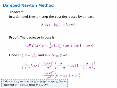
Damped Newton Method
Theorem:
In a damped Newton step the cost decreases by at least
λt(x)− log(1+ λt(x))
Proof: The decrease in cost is
−α∇ft(x)Tv + 1σ2 ‖v‖2
Hx(ασ + log(1−ασ))
Choosing α = 11+σ and v = ∆xnt gives
11+ σ λt(x)
2+λt(x)2
σ2
(σ
1+ σ + log(1− σ
1+ σ))
=λt(x)2
σ2
(σ − log(1+ σ)
)
With v = ∆xnt we have ‖w‖2 = ‖v‖Hx = λt(x); furtherrecall that σ = ‖w‖∞; hence σ ≤ λt(x).
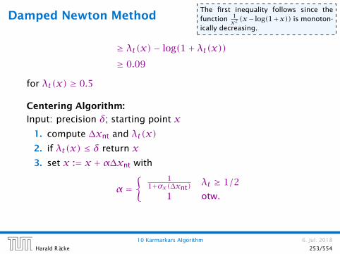
Damped Newton Method
≥ λt(x)− log(1+ λt(x))≥ 0.09
for λt(x) ≥ 0.5
Centering Algorithm:
Input: precision δ; starting point x1. compute ∆xnt and λt(x)2. if λt(x) ≤ δ return x3. set x := x +α∆xnt with
α = 1
1+σx(∆xnt)λt ≥ 1/2
1 otw.
The first inequality follows since thefunction 1
x2 (x− log(1+x)) is monoton-ically decreasing.
10 Karmarkars Algorithm 6. Jul. 2018
Harald Räcke 253/554

Centering
Lemma 56
The centering algorithm starting at x0 reaches a point with
λt(x) ≤ δ after
ft(x0)−miny ft(y)0.09
+O(log log(1/δ))
iterations.
This can be very, very slow...
10 Karmarkars Algorithm 6. Jul. 2018
Harald Räcke 254/554

How to get close to analytic center?
Let P = Ax ≤ b be our (feasible) polyhedron, and x0 a feasible
point.
We change b → b + 1λ · ~1, where L = 〈A〉 + 〈b〉 + 〈c〉 (encoding
length) and λ = 22L. Recall that a basis is feasible in the old LP
iff it is feasible in the new LP.
10 Karmarkars Algorithm 6. Jul. 2018
Harald Räcke 255/554

Lemma [without proof]
The inverse of a matrix M can be represented with rational
numbers that have denominators zij = det(M).
For two basis solutions xB, xB, the cost-difference cTxB − cTxBcan be represented by a rational number that has denominator
z = det(AB) · det(AB).
This means that in the perturbed LP it is sufficient to decrease
the duality gap to 1/24L (i.e., t ≈ 24L). This means the previous
analysis essentially also works for the perturbed LP.
For a point x from the polytope (not necessarily BFS) the
objective value cTx is at most n2M2L, where M ≤ L is the
encoding length of the largest entry in c.
10 Karmarkars Algorithm 6. Jul. 2018
Harald Räcke 256/554
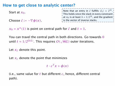
How to get close to analytic center?Note that an entry in c fulfills |ci| ≤ 22L.This holds since the slack in every constraintat x0 is at least λ = 1/22L, and the gradientis the vector of inverse slacks.
Start at x0.
Choose c := −∇φ(x).
x0 = x∗(1) is point on central path for c and t = 1.
You can travel the central path in both directions. Go towards 0
until t ≈ 1/2Ω(L). This requires O(√mL) outer iterations.
Let xc denote this point.
Let xc denote the point that minimizes
t · cTx +φ(x)
(i.e., same value for t but different c, hence, different central
path).

How to get close to analytic center?
Clearly,
t · cTxc +φ(xc) ≤ t · cTxc +φ(xc)
The difference between ft(xc) and ft(xc) is
tcTxc +φ(xc)− tcTxc −φ(xc)≤ t(cTxc + cTxc − cTxc − cTxc)≤ 4tn23L
For t = 1/2Ω(L) the last term becomes constant. Hence, using
damped Newton we can move from xc to xc quickly.
In total for this analysis we require O(√mL) outer iterations for
the whole algorithm.
One iteration can be implemented in O(m3) time.

Part III
Approximation Algorithms
6. Jul. 2018
Harald Räcke 259/554

There are many practically important optimization problems that
are NP-hard.
What can we do?
ñ Heuristics.
ñ Exploit special structure of instances occurring in practise.
ñ Consider algorithms that do not compute the optimal
solution but provide solutions that are close to optimum.
11 Introduction to Approximation 6. Jul. 2018
Harald Räcke 260/554

Definition 57
An α-approximation for an optimization problem is a
polynomial-time algorithm that for all instances of the problem
produces a solution whose value is within a factor of α of the
value of an optimal solution.
11 Introduction to Approximation 6. Jul. 2018
Harald Räcke 261/554

Why approximation algorithms?
ñ We need algorithms for hard problems.
ñ It gives a rigorous mathematical base for studying
heuristics.
ñ It provides a metric to compare the difficulty of various
optimization problems.
ñ Proving theorems may give a deeper theoretical
understanding which in turn leads to new algorithmic
approaches.
Why not?
ñ Sometimes the results are very pessimistic due to the fact
that an algorithm has to provide a close-to-optimum
solution on every instance.
11 Introduction to Approximation 6. Jul. 2018
Harald Räcke 262/554

Definition 58
An optimization problem P = (I, sol,m,goal) is in NPO if
ñ x ∈ I can be decided in polynomial time
ñ y ∈ sol(I) can be verified in polynomial time
ñ m can be computed in polynomial time
ñ goal ∈ min,max
In other words: the decision problem is there a solution y with
m(x,y) at most/at least z is in NP.
11 Introduction to Approximation 6. Jul. 2018
Harald Räcke 263/554
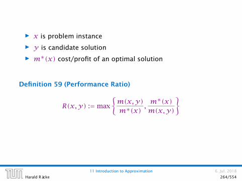
ñ x is problem instance
ñ y is candidate solution
ñ m∗(x) cost/profit of an optimal solution
Definition 59 (Performance Ratio)
R(x,y) :=max
m(x,y)m∗(x)
,m∗(x)m(x,y)
11 Introduction to Approximation 6. Jul. 2018
Harald Räcke 264/554

Definition 60 (r -approximation)
An algorithm A is an r -approximation algorithm iff
∀x ∈ I : R(x,A(x)) ≤ r ,
and A runs in polynomial time.
11 Introduction to Approximation 6. Jul. 2018
Harald Räcke 265/554

Definition 61 (PTAS)
A PTAS for a problem P from NPO is an algorithm that takes as
input x ∈ I and ε > 0 and produces a solution y for x with
R(x,y) ≤ 1+ ε .
The running time is polynomial in |x|.
approximation with arbitrary good factor... fast?
11 Introduction to Approximation 6. Jul. 2018
Harald Räcke 266/554

Problems that have a PTAS
Scheduling. Given m jobs with known processing times; schedule
the jobs on n machines such that the MAKESPAN is minimized.
11 Introduction to Approximation 6. Jul. 2018
Harald Räcke 267/554

Definition 62 (FPTAS)
An FPTAS for a problem P from NPO is an algorithm that takes
as input x ∈ I and ε > 0 and produces a solution y for x with
R(x,y) ≤ 1+ ε .
The running time is polynomial in |x| and 1/ε.
approximation with arbitrary good factor... fast!
11 Introduction to Approximation 6. Jul. 2018
Harald Räcke 268/554

Problems that have an FPTAS
KNAPSACK. Given a set of items with profits and weights choose a
subset of total weight at most W s.t. the profit is maximized.
11 Introduction to Approximation 6. Jul. 2018
Harald Räcke 269/554

Definition 63 (APX – approximable)
A problem P from NPO is in APX if there exist a constant r ≥ 1
and an r -approximation algorithm for P .
constant factor approximation...
11 Introduction to Approximation 6. Jul. 2018
Harald Räcke 270/554

Problems that are in APX
MAXCUT. Given a graph G = (V , E); partition V into two disjointpieces A and B s. t. the number of edges between both pieces ismaximized.
MAX-3SAT. Given a 3CNF-formula. Find an assignment to the
variables that satisfies the maximum number of clauses.
11 Introduction to Approximation 6. Jul. 2018
Harald Räcke 271/554

Problems with polylogarithmic approximation guarantees
ñ Set Cover
ñ Minimum Multicut
ñ Sparsest Cut
ñ Minimum Bisection
There is an r -approximation with r ≤ O(logc(|x|)) for some
constant c.
Note that only for some of the above problem a matching lower
bound is known.
11 Introduction to Approximation 6. Jul. 2018
Harald Räcke 272/554

There are really difficult problems!
Theorem 64
For any constant ε > 0 there does not exist an
Ω(n1−ε)-approximation algorithm for the maximum clique
problem on a given graph G with n nodes unless P = NP.
Note that an n-approximation is trivial.
11 Introduction to Approximation 6. Jul. 2018
Harald Räcke 273/554

There are weird problems!
Asymmetric k-Center admits an O(log∗n)-approximation.
There is no o(log∗n)-approximation to Asymmetric k-Center
unless NP ⊆ DTIME(nlog log logn).
11 Introduction to Approximation 6. Jul. 2018
Harald Räcke 274/554

Class APX not important in practise.
Instead of saying problem P is in APX one says problem Padmits a 4-approximation.
One only says that a problem is APX-hard.
11 Introduction to Approximation 6. Jul. 2018
Harald Räcke 275/554

A crucial ingredient for the design and analysis of approximation
algorithms is a technique to obtain an upper bound (for
maximization problems) or a lower bound (for minimization
problems).
Therefore Linear Programs or Integer Linear Programs play a
vital role in the design of many approximation algorithms.
12 Integer Programs 6. Jul. 2018
Harald Räcke 276/554

Definition 65
An Integer Linear Program or Integer Program is a Linear
Program in which all variables are required to be integral.
Definition 66
A Mixed Integer Program is a Linear Program in which a subset
of the variables are required to be integral.
12 Integer Programs 6. Jul. 2018
Harald Räcke 277/554
Many important combinatorial optimization problems can be
formulated in the form of an Integer Program.
Note that solving Integer Programs in general is
NP-complete!
12 Integer Programs 6. Jul. 2018
Harald Räcke 278/554

Set Cover
Given a ground set U , a collection of subsets S1, . . . , Sk ⊆ U ,
where the i-th subset Si has weight/cost wi. Find a collection
I ⊆ 1, . . . , k such that
∀u ∈ U∃i ∈ I : u ∈ Si (every element is covered)
and ∑
i∈Iwi is minimized.
12 Integer Programs 6. Jul. 2018
Harald Räcke 279/554

Set Cover
12 Integer Programs 6. Jul. 2018
Harald Räcke 280/554
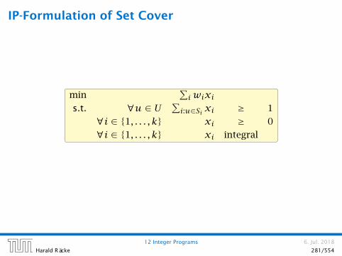
IP-Formulation of Set Cover
min∑iwixi
s.t. ∀u ∈ U ∑i:u∈Si xi ≥ 1
∀i ∈ 1, . . . , k xi ≥ 0
∀i ∈ 1, . . . , k xi integral
12 Integer Programs 6. Jul. 2018
Harald Räcke 281/554

Vertex Cover
Given a graph G = (V , E) and a weight wv for every node. Find a
vertex subset S ⊆ V of minimum weight such that every edge is
incident to at least one vertex in S.
12 Integer Programs 6. Jul. 2018
Harald Räcke 282/554
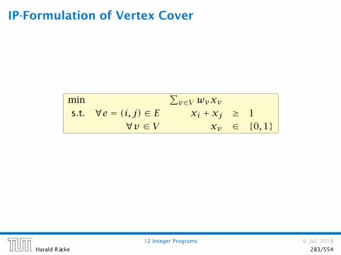
IP-Formulation of Vertex Cover
min∑v∈V wvxv
s.t. ∀e = (i, j) ∈ E xi + xj ≥ 1
∀v ∈ V xv ∈ 0,1
12 Integer Programs 6. Jul. 2018
Harald Räcke 283/554

Maximum Weighted Matching
Given a graph G = (V , E), and a weight we for every edge e ∈ E.
Find a subset of edges of maximum weight such that no vertex
is incident to more than one edge.
max∑e∈Ewexe
s.t. ∀v ∈ V ∑e:v∈e xe ≤ 1
∀e ∈ E xe ∈ 0,1
12 Integer Programs 6. Jul. 2018
Harald Räcke 284/554

Maximum Independent Set
Given a graph G = (V , E), and a weight wv for every node v ∈ V .
Find a subset S ⊆ V of nodes of maximum weight such that no
two vertices in S are adjacent.
max∑v∈V wvxv
s.t. ∀e = (i, j) ∈ E xi + xj ≤ 1
∀v ∈ V xv ∈ 0,1
12 Integer Programs 6. Jul. 2018
Harald Räcke 285/554

Knapsack
Given a set of items 1, . . . , n, where the i-th item has weight
wi and profit pi, and given a threshold K. Find a subset
I ⊆ 1, . . . , n of items of total weight at most K such that the
profit is maximized.
max∑ni=1 pixi
s.t.∑ni=1wixi ≤ K
∀i ∈ 1, . . . , n xi ∈ 0,1
12 Integer Programs 6. Jul. 2018
Harald Räcke 286/554

Relaxations
Definition 67
A linear program LP is a relaxation of an integer program IP if
any feasible solution for IP is also feasible for LP and if the
objective values of these solutions are identical in both
programs.
We obtain a relaxation for all examples by writing xi ∈ [0,1]instead of xi ∈ 0,1.
12 Integer Programs 6. Jul. 2018
Harald Räcke 287/554

By solving a relaxation we obtain an upper bound for a
maximization problem and a lower bound for a minimization
problem.
12 Integer Programs 6. Jul. 2018
Harald Räcke 288/554

Relations
Maximization Problems:
OPT(IP) OPT(LP)
OPT(DUAL)ALG(IP) FEASIBLE(DUAL)
0
Minimization Problems:
OPT(IP)OPT(LP)
OPT(DUAL) ALG(IP)FEASIBLE(DUAL)
0
12 Integer Programs 6. Jul. 2018
Harald Räcke 289/554

Technique 1: Round the LP solution.
We first solve the LP-relaxation and then we round the fractional
values so that we obtain an integral solution.
Set Cover relaxation:
min∑ki=1wixi
s.t. ∀u ∈ U ∑i:u∈Si xi ≥ 1
∀i ∈ 1, . . . , k xi ∈ [0,1]
Let fu be the number of sets that the element u is contained in
(the frequency of u). Let f =maxufu be the maximum
frequency.
13.1 Deterministic Rounding 6. Jul. 2018
Harald Räcke 290/554

Technique 1: Round the LP solution.
Rounding Algorithm:
Set all xi-values with xi ≥ 1f to 1. Set all other xi-values to 0.
13.1 Deterministic Rounding 6. Jul. 2018
Harald Räcke 291/554

Technique 1: Round the LP solution.
Lemma 68
The rounding algorithm gives an f -approximation.
Proof: Every u ∈ U is covered.
ñ We know that∑i:u∈Si xi ≥ 1.
ñ The sum contains at most fu ≤ f elements.
ñ Therefore one of the sets that contain u must have xi ≥ 1/f .ñ This set will be selected. Hence, u is covered.
13.1 Deterministic Rounding 6. Jul. 2018
Harald Räcke 292/554

Technique 1: Round the LP solution.
The cost of the rounded solution is at most f ·OPT.
∑
i∈Iwi ≤
k∑
i=1
wi(f · xi)
= f · cost(x)
≤ f ·OPT .
13.1 Deterministic Rounding 6. Jul. 2018
Harald Räcke 293/554

Technique 2: Rounding the Dual Solution.
Relaxation for Set Cover
Primal:
min∑i∈Iwixi
s.t. ∀u ∑i:u∈Si xi ≥ 1
xi ≥ 0
Dual:
max∑u∈U yu
s.t. ∀i ∑u:u∈Si yu ≤ wiyu ≥ 0
13.2 Rounding the Dual 6. Jul. 2018
Harald Räcke 294/554
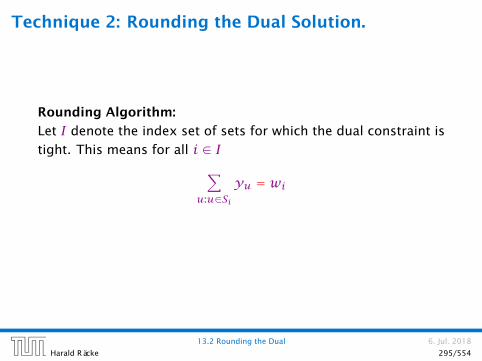
Technique 2: Rounding the Dual Solution.
Rounding Algorithm:
Let I denote the index set of sets for which the dual constraint is
tight. This means for all i ∈ I∑
u:u∈Siyu = wi
13.2 Rounding the Dual 6. Jul. 2018
Harald Räcke 295/554

Technique 2: Rounding the Dual Solution.
Lemma 69
The resulting index set is an f -approximation.
Proof:
Every u ∈ U is covered.
ñ Suppose there is a u that is not covered.
ñ This means∑u:u∈Si yu < wi for all sets Si that contain u.
ñ But then yu could be increased in the dual solution without
violating any constraint. This is a contradiction to the fact
that the dual solution is optimal.
13.2 Rounding the Dual 6. Jul. 2018
Harald Räcke 296/554

Technique 2: Rounding the Dual Solution.
Proof:
∑
i∈Iwi =
∑
i∈I
∑
u:u∈Siyu
=∑u|i ∈ I : u ∈ Si| ·yu
≤∑ufuyu
≤ f∑uyu
≤ fcost(x∗)
≤ f ·OPT
13.2 Rounding the Dual 6. Jul. 2018
Harald Räcke 297/554

Let I denote the solution obtained by the first rounding
algorithm and I′ be the solution returned by the second
algorithm. Then
I ⊆ I′ .This means I′ is never better than I.
ñ Suppose that we take Si in the first algorithm. I.e., i ∈ I.ñ This means xi ≥ 1
f .
ñ Because of Complementary Slackness Conditions the
corresponding constraint in the dual must be tight.
ñ Hence, the second algorithm will also choose Si.
13.2 Rounding the Dual 6. Jul. 2018
Harald Räcke 298/554

Technique 3: The Primal Dual Method
The previous two rounding algorithms have the disadvantage
that it is necessary to solve the LP. The following method also
gives an f -approximation without solving the LP.
For estimating the cost of the solution we only required two
properties.
1. The solution is dual feasible and, hence,
∑uyu ≤ cost(x∗) ≤ OPT
where x∗ is an optimum solution to the primal LP.
2. The set I contains only sets for which the dual inequality is
tight.
Of course, we also need that I is a cover.
13.3 Primal Dual Technique 6. Jul. 2018
Harald Räcke 299/554

Technique 3: The Primal Dual Method
Algorithm 1 PrimalDual1: y ← 0
2: I ← 3: while exists u ∉
⋃i∈I Si do
4: increase dual variable yu until constraint for some
new set S` becomes tight
5: I ← I ∪ `
13.3 Primal Dual Technique 6. Jul. 2018
Harald Räcke 300/554

Technique 4: The Greedy Algorithm
Algorithm 1 Greedy
1: I ← 2: Sj ← Sj for all j3: while I not a set cover do
4: ` ← arg minj:Sj≠0wj|Sj|
5: I ← I ∪ `6: Sj ← Sj − S` for all j
In every round the Greedy algorithm takes the set that covers
remaining elements in the most cost-effective way.
We choose a set such that the ratio between cost and still
uncovered elements in the set is minimized.
13.4 Greedy 6. Jul. 2018
Harald Räcke 301/554

Technique 4: The Greedy Algorithm
Lemma 70
Given positive numbers a1, . . . , ak and b1, . . . , bk, and
S ⊆ 1, . . . , k then
mini
aibi≤∑i∈S ai∑i∈S bi
≤maxi
aibi
13.4 Greedy 6. Jul. 2018
Harald Räcke 302/554

Technique 4: The Greedy Algorithm
Let n` denote the number of elements that remain at the
beginning of iteration `. n1 = n = |U| and ns+1 = 0 if we need siterations.
In the `-th iteration
minj
wj|Sj|
≤∑j∈OPTwj∑j∈OPT |Sj|
= OPT∑j∈OPT |Sj|
≤ OPTn`
since an optimal algorithm can cover the remaining n` elements
with cost OPT.
Let Sj be a subset that minimizes this ratio. Hence,
wj/|Sj| ≤ OPTn`
.
13.4 Greedy 6. Jul. 2018
Harald Räcke 303/554

Technique 4: The Greedy Algorithm
Adding this set to our solution means n`+1 = n` − |Sj|.
wj ≤|Sj|OPT
n`= n` −n`+1
n`·OPT
13.4 Greedy 6. Jul. 2018
Harald Räcke 304/554

Technique 4: The Greedy Algorithm
∑
j∈Iwj ≤
s∑
`=1
n` −n`+1
n`·OPT
≤ OPTs∑
`=1
(1n`+ 1n` − 1
+ · · · + 1n`+1 + 1
)
= OPTn∑
i=1
1i
= Hn ·OPT ≤ OPT(lnn+ 1) .
13.4 Greedy 6. Jul. 2018
Harald Räcke 305/554

Technique 4: The Greedy Algorithm
A tight example:
1 12
13
14
1 + ε
1n−1
1n−2
1n−3
1n
13.4 Greedy 6. Jul. 2018
Harald Räcke 306/554

Technique 5: Randomized Rounding
One round of randomized rounding:
Pick set Sj uniformly at random with probability 1−xj (for all j).
Version A: Repeat rounds until you nearly have a cover. Cover
remaining elements by some simple heuristic.
Version B: Repeat for s rounds. If you have a cover STOP.
Otherwise, repeat the whole algorithm.
13.5 Randomized Rounding 6. Jul. 2018
Harald Räcke 307/554

Probability that u ∈ U is not covered (in one round):
Pr[u not covered in one round]
=∏
j:u∈Sj(1− xj) ≤
∏
j:u∈Sje−xj
= e−∑j:u∈Sj xj ≤ e−1 .
Probability that u ∈ U is not covered (after ` rounds):
Pr[u not covered after ` round] ≤ 1
e`.
13.5 Randomized Rounding 6. Jul. 2018
Harald Räcke 308/554

Pr[∃u ∈ U not covered after ` round]
= Pr[u1 not covered∨ u2 not covered∨ . . .∨ un not covered]
≤∑
iPr[ui not covered after ` rounds] ≤ ne−` .
Lemma 71
With high probability O(logn) rounds suffice.
With high probability:
For any constant α the number of rounds is at most O(logn)with probability at least 1−n−α.
13.5 Randomized Rounding 6. Jul. 2018
Harald Räcke 309/554

Proof: We have
Pr[#rounds ≥ (α+ 1) lnn] ≤ ne−(α+1) lnn = n−α .
13.5 Randomized Rounding 6. Jul. 2018
Harald Räcke 310/554

Expected Cost
ñ Version A.
Repeat for s = (α+ 1) lnn rounds. If you don’t have a cover
simply take for each element u the cheapest set that
contains u.
E[cost] ≤ (α+1) lnn·cost(LP)+(n·OPT)n−α = O(lnn)·OPT
13.5 Randomized Rounding 6. Jul. 2018
Harald Räcke 311/554
Expected Cost
ñ Version B.Repeat for s = (α+ 1) lnn rounds. If you don’t have a coversimply repeat the whole process.
E[cost] = Pr[success] · E[cost | success]
+ Pr[no success] · E[cost | no success]
This means
E[cost | success]
= 1Pr[succ.]
(E[cost]− Pr[no success] · E[cost | no success]
)
≤ 1Pr[succ.]
E[cost] ≤ 11−n−α (α+ 1) lnn · cost(LP)
≤ 2(α+ 1) lnn ·OPT
for n ≥ 2 and α ≥ 1.
13.5 Randomized Rounding 6. Jul. 2018
Harald Räcke 312/554

Randomized rounding gives an O(logn) approximation. The
running time is polynomial with high probability.
Theorem 72 (without proof)
There is no approximation algorithm for set cover with
approximation guarantee better than 12 logn unless NP has
quasi-polynomial time algorithms (algorithms with running time
2poly(logn)).
13.5 Randomized Rounding 6. Jul. 2018
Harald Räcke 313/554

Integrality Gap
The integrality gap of the SetCover LP is Ω(logn).
ñ n = 2k − 1
ñ Elements are all vectors ~x over GF[2] of length k (excluding
zero vector).
ñ Every vector ~y defines a set as follows
S~y := ~x | ~xT ~y = 1
ñ each set contains 2k−1 vectors; each vector is contained in
2k−1 sets
ñ xi = 12k−1 = 2
n+1 is fractional solution.
13.5 Randomized Rounding 6. Jul. 2018
Harald Räcke 314/554

Integrality Gap
Every collection of p < k sets does not cover all elements.
Hence, we get a gap of Ω(logn).
13.5 Randomized Rounding 6. Jul. 2018
Harald Räcke 315/554

Techniques:
ñ Deterministic Rounding
ñ Rounding of the Dual
ñ Primal Dual
ñ Greedy
ñ Randomized Rounding
ñ Local Search
ñ Rounding Data + Dynamic Programming
13.5 Randomized Rounding 6. Jul. 2018
Harald Räcke 316/554

Scheduling Jobs on Identical Parallel Machines
Given n jobs, where job j ∈ 1, . . . , n has processing time pj.Schedule the jobs on m identical parallel machines such that the
Makespan (finishing time of the last job) is minimized.
min Ls.t. ∀machines i
∑j pj · xj,i ≤ L
∀jobs j∑i xj,i ≥ 1
∀i, j xj,i ∈ 0,1
Here the variable xj,i is the decision variable that describes
whether job j is assigned to machine i.
14.1 Local Search 6. Jul. 2018
Harald Räcke 317/554

Lower Bounds on the Solution
Let for a given schedule Cj denote the finishing time of machine
j, and let Cmax be the makespan.
Let C∗max denote the makespan of an optimal solution.
Clearly
C∗max ≥maxjpj
as the longest job needs to be scheduled somewhere.
14.1 Local Search 6. Jul. 2018
Harald Räcke 318/554

Lower Bounds on the Solution
The average work performed by a machine is 1m∑j pj.
Therefore,
C∗max ≥1m
∑
jpj
14.1 Local Search 6. Jul. 2018
Harald Räcke 319/554

Local Search
A local search algorithm successively makes certain small
(cost/profit improving) changes to a solution until it does not
find such changes anymore.
It is conceptionally very different from a Greedy algorithm as a
feasible solution is always maintained.
Sometimes the running time is difficult to prove.
14.1 Local Search 6. Jul. 2018
Harald Räcke 320/554

Local Search for Scheduling
Local Search Strategy: Take the job that finishes last and try to
move it to another machine. If there is such a move that reduces
the makespan, perform the switch.
REPEAT
14.1 Local Search 6. Jul. 2018
Harald Räcke 321/554

Local Search Analysis
Let ` be the job that finishes last in the produced schedule.
Let S` be its start time, and let C` be its completion time.
Note that every machine is busy before time S`, because
otherwise we could move the job ` and hence our schedule
would not be locally optimal.
14.1 Local Search 6. Jul. 2018
Harald Räcke 322/554

We can split the total processing time into two intervals one
from 0 to S` the other from S` to C`.
The interval [S`, C`] is of length p` ≤ C∗max.
During the first interval [0, S`] all processors are busy, and,
hence, the total work performed in this interval is
m · S` ≤∑
j≠`
pj .
Hence, the length of the schedule is at most
p` +1m
∑
j≠`
pj = (1− 1m)p` +
1m
∑
jpj ≤ (2− 1
m)C∗max
14.1 Local Search 6. Jul. 2018
Harald Räcke 323/554

A Tight Example
p` ≈ S` +S`
m− 1
ALGOPT
= S` + p`p`
≈ 2+ 1m−1
1+ 1m−1
= 2− 1m
p`
p`
S`

A Greedy Strategy
List Scheduling:
Order all processes in a list. When a machine runs empty assign
the next yet unprocessed job to it.
Alternatively:
Consider processes in some order. Assign the i-th process to the
least loaded machine.
It is easy to see that the result of these greedy strategies fulfill
the local optimally condition of our local search algorithm.
Hence, these also give 2-approximations.
14.2 Greedy 6. Jul. 2018
Harald Räcke 325/554

A Greedy Strategy
Lemma 73
If we order the list according to non-increasing processing times
the approximation guarantee of the list scheduling strategy
improves to 4/3.
14.2 Greedy 6. Jul. 2018
Harald Räcke 326/554
Proof:
ñ Let p1 ≥ · · · ≥ pn denote the processing times of a set of
jobs that form a counter-example.
ñ Wlog. the last job to finish is n (otw. deleting this job gives
another counter-example with fewer jobs).
ñ If pn ≤ C∗max/3 the previous analysis gives us a schedule
length of at most
C∗max + pn ≤43C∗max .
Hence, pn > C∗max/3.
ñ This means that all jobs must have a processing time
> C∗max/3.
ñ But then any machine in the optimum schedule can handle
at most two jobs.
ñ For such instances Longest-Processing-Time-First is optimal.
14.2 Greedy 6. Jul. 2018
Harald Räcke 327/554

When in an optimal solution a machine can have at most 2 jobs
the optimal solution looks as follows.
p1 p2 p3 p4 p5 p6 p7
p8p9p10p11p12p13p14
14.2 Greedy 6. Jul. 2018
Harald Räcke 328/554

ñ We can assume that one machine schedules p1 and pn (the
largest and smallest job).
ñ If not assume wlog. that p1 is scheduled on machine A and
pn on machine B.
ñ Let pA and pB be the other job scheduled on A and B,
respectively.
ñ p1 +pn ≤ p1 +pA and pA +pB ≤ p1 +pA, hence scheduling
p1 and pn on one machine and pA and pB on the other,
cannot increase the Makespan.
ñ Repeat the above argument for the remaining machines.
14.2 Greedy 6. Jul. 2018
Harald Räcke 329/554

Tight Example
ñ 2m+ 1 jobs
ñ 2 jobs with length 2m,2m− 1,2m− 2, . . . ,m+ 1 (2m− 2
jobs in total)
ñ 3 jobs of length m
14.2 Greedy 6. Jul. 2018
Harald Räcke 330/554

15 Rounding Data + Dynamic Programming
Knapsack:
Given a set of items 1, . . . , n, where the i-th item has weight
wi ∈ N and profit pi ∈ N, and given a threshold W . Find a
subset I ⊆ 1, . . . , n of items of total weight at most W such
that the profit is maximized (we can assume each wi ≤ W ).
max∑ni=1 pixi
s.t.∑ni=1wixi ≤ W
∀i ∈ 1, . . . , n xi ∈ 0,1
15.1 Knapsack 6. Jul. 2018
Harald Räcke 331/554

15 Rounding Data + Dynamic Programming
Algorithm 1 Knapsack
1: A(1)← [(0,0), (p1,w1)]2: for j ← 2 to n do
3: A(j)← A(j − 1)4: for each (p,w) ∈ A(j − 1) do
5: if w +wj ≤ W then
6: add (p + pj ,w +wj) to A(j)7: remove dominated pairs from A(j)8: return max(p,w)∈A(n) p
The running time is O(n ·minW,P), where P =∑i pi is the
total profit of all items. This is only pseudo-polynomial.
15.1 Knapsack 6. Jul. 2018
Harald Räcke 332/554

15 Rounding Data + Dynamic Programming
Definition 74
An algorithm is said to have pseudo-polynomial running time if
the running time is polynomial when the numerical part of the
input is encoded in unary.
15.1 Knapsack 6. Jul. 2018
Harald Räcke 333/554

15 Rounding Data + Dynamic Programming
ñ Let M be the maximum profit of an element.
ñ Set µ := εM/n.
ñ Set p′i := bpi/µc for all i.ñ Run the dynamic programming algorithm on this revised
instance.
Running time is at most
O(nP ′) = O(n∑i p′i
)= O
(n∑i
⌊ piεM/n
⌋)≤ O
(n3
ε
).
15.1 Knapsack 6. Jul. 2018
Harald Räcke 334/554
15 Rounding Data + Dynamic Programming
Let S be the set of items returned by the algorithm, and let O be
an optimum set of items.∑
i∈Spi ≥ µ
∑
i∈Sp′i
≥ µ∑
i∈Op′i
≥∑
i∈Opi − |O|µ
≥∑
i∈Opi −nµ
=∑
i∈Opi − εM
≥ (1− ε)OPT .
15.1 Knapsack 6. Jul. 2018
Harald Räcke 335/554
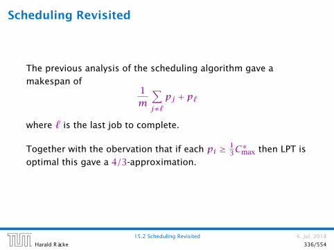
Scheduling Revisited
The previous analysis of the scheduling algorithm gave a
makespan of1m
∑
j≠`
pj + p`
where ` is the last job to complete.
Together with the obervation that if each pi ≥ 13C∗max then LPT is
optimal this gave a 4/3-approximation.
15.2 Scheduling Revisited 6. Jul. 2018
Harald Räcke 336/554

15.2 Scheduling Revisited
Partition the input into long jobs and short jobs.
A job j is called short if
pj ≤ 1km
∑i pi
Idea:
1. Find the optimum Makespan for the long jobs by brute
force.
2. Then use the list scheduling algorithm for the short jobs,
always assigning the next job to the least loaded machine.
15.2 Scheduling Revisited 6. Jul. 2018
Harald Räcke 337/554

We still have a cost of
1m
∑
j≠`
pj + p`
where ` is the last job (this only requires that all machines are
busy before time S`).
If ` is a long job, then the schedule must be optimal, as it
consists of an optimal schedule of long jobs plus a schedule for
short jobs.
If ` is a short job its length is at most
p` ≤∑j pj/(mk)
which is at most C∗max/k.
15.2 Scheduling Revisited 6. Jul. 2018
Harald Räcke 338/554

Hence we get a schedule of length at most
(1+ 1
k
)C∗max
There are at most km long jobs. Hence, the number of
possibilities of scheduling these jobs on m machines is at most
mkm, which is constant if m is constant. Hence, it is easy to
implement the algorithm in polynomial time.
Theorem 75
The above algorithm gives a polynomial time approximation
scheme (PTAS) for the problem of scheduling n jobs on midentical machines if m is constant.
We choose k = d1ε e.
15.2 Scheduling Revisited 6. Jul. 2018
Harald Räcke 339/554

How to get rid of the requirement that m is constant?
We first design an algorithm that works as follows:
On input of T it either finds a schedule of length (1+ 1k)T or
certifies that no schedule of length at most T exists (assume
T ≥ 1m∑j pj).
We partition the jobs into long jobs and short jobs:
ñ A job is long if its size is larger than T/k.
ñ Otw. it is a short job.
15.2 Scheduling Revisited 6. Jul. 2018
Harald Räcke 340/554

ñ We round all long jobs down to multiples of T/k2.
ñ For these rounded sizes we first find an optimal schedule.
ñ If this schedule does not have length at most T we conclude
that also the original sizes don’t allow such a schedule.
ñ If we have a good schedule we extend it by adding the short
jobs according to the LPT rule.
15.2 Scheduling Revisited 6. Jul. 2018
Harald Räcke 341/554

After the first phase the rounded sizes of the long jobs assigned
to a machine add up to at most T .
There can be at most k (long) jobs assigned to a machine as otw.
their rounded sizes would add up to more than T (note that the
rounded size of a long job is at least T/k).
Since, jobs had been rounded to multiples of T/k2 going from
rounded sizes to original sizes gives that the Makespan is at
most (1+ 1
k
)T .
15.2 Scheduling Revisited 6. Jul. 2018
Harald Räcke 342/554

During the second phase there always must exist a machine with
load at most T , since T is larger than the average load.
Assigning the current (short) job to such a machine gives that
the new load is at most
T + Tk≤(1+ 1
k
)T .
15.2 Scheduling Revisited 6. Jul. 2018
Harald Räcke 343/554

Running Time for scheduling large jobs: There should not be
a job with rounded size more than T as otw. the problem
becomes trivial.
Hence, any large job has rounded size of ik2T for i ∈ k, . . . , k2.
Therefore the number of different inputs is at most nk2
(described by a vector of length k2 where, the i-th entry
describes the number of jobs of size ik2T ). This is polynomial.
The schedule/configuration of a particular machine x can be
described by a vector of length k2 where the i-th entry describes
the number of jobs of rounded size ik2T assigned to x. There
are only (k+ 1)k2different vectors.
This means there are a constant number of different machine
configurations.
15.2 Scheduling Revisited 6. Jul. 2018
Harald Räcke 344/554

Let OPT(n1, . . . , nk2) be the number of machines that are
required to schedule input vector (n1, . . . , nk2) with Makespan at
most T .
If OPT(n1, . . . , nk2) ≤ m we can schedule the input.
We have
OPT(n1, . . . , nk2)
=
0 (n1, . . . , nk2) = 01+ min
(s1,...,sk2 )∈COPT(n1 − s1, . . . , nk2 − sk2) (n1, . . . , nk2) Û 0
∞ otw.
where C is the set of all configurations.
Hence, the running time is roughly (k+ 1)k2nk2 ≈ (nk)k2.
15.2 Scheduling Revisited 6. Jul. 2018
Harald Räcke 345/554

We can turn this into a PTAS by choosing k = d1/εe and using
binary search. This gives a running time that is exponential in
1/ε.
Can we do better?
Scheduling on identical machines with the goal of minimizing
Makespan is a strongly NP-complete problem.
Theorem 76
There is no FPTAS for problems that are strongly NP-hard.
15.2 Scheduling Revisited 6. Jul. 2018
Harald Räcke 346/554

ñ Suppose we have an instance with polynomially bounded
processing times pi ≤ q(n)ñ We set k := d2nq(n)e ≥ 2 OPT
ñ Then
ALG ≤(1+ 1
k
)OPT ≤ OPT+1
2
ñ But this means that the algorithm computes the optimal
solution as the optimum is integral.
ñ This means we can solve problem instances if processing
times are polynomially bounded
ñ Running time is O(poly(n, k)) = O(poly(n))ñ For strongly NP-complete problems this is not possible
unless P=NP
15.2 Scheduling Revisited 6. Jul. 2018
Harald Räcke 347/554

More GeneralLet OPT(n1, . . . , nA) be the number of machines that are required toschedule input vector (n1, . . . , nA) with Makespan at most T(A: number of different sizes).
If OPT(n1, . . . , nA) ≤m we can schedule the input.
OPT(n1, . . . , nA)
=
0 (n1, . . . , nA) = 01+ min
(s1,...,sA)∈COPT(n1 − s1, . . . , nA − sA) (n1, . . . , nA) Û 0
∞ otw.
where C is the set of all configurations.
|C| ≤ (B + 1)A, where B is the number of jobs that possibly can fit onthe same machine.
The running time is then O((B + 1)AnA) because the dynamic
programming table has just nA entries.
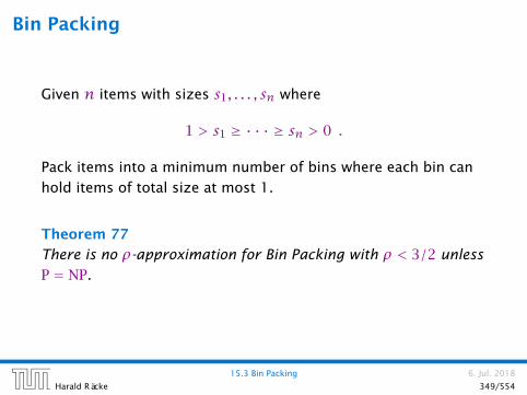
Bin Packing
Given n items with sizes s1, . . . , sn where
1 > s1 ≥ · · · ≥ sn > 0 .
Pack items into a minimum number of bins where each bin can
hold items of total size at most 1.
Theorem 77
There is no ρ-approximation for Bin Packing with ρ < 3/2 unless
P = NP.
15.3 Bin Packing 6. Jul. 2018
Harald Räcke 349/554

Bin Packing
Proof
ñ In the partition problem we are given positive integers
b1, . . . , bn with B =∑i bi even. Can we partition the integers
into two sets S and T s.t.
∑
i∈Sbi =
∑
i∈Tbi ?
ñ We can solve this problem by setting si := 2bi/B and asking
whether we can pack the resulting items into 2 bins or not.
ñ A ρ-approximation algorithm with ρ < 3/2 cannot output 3
or more bins when 2 are optimal.
ñ Hence, such an algorithm can solve Partition.
15.3 Bin Packing 6. Jul. 2018
Harald Räcke 350/554

Bin Packing
Definition 78
An asymptotic polynomial-time approximation scheme (APTAS)
is a family of algorithms Aε along with a constant c such that
Aε returns a solution of value at most (1+ ε)OPT+ c for
minimization problems.
ñ Note that for Set Cover or for Knapsack it makes no sense
to differentiate between the notion of a PTAS or an APTAS
because of scaling.
ñ However, we will develop an APTAS for Bin Packing.
15.3 Bin Packing 6. Jul. 2018
Harald Räcke 351/554

Bin Packing
Again we can differentiate between small and large items.
Lemma 79
Any packing of items into ` bins can be extended with items of
size at most γ s.t. we use only max`, 11−γ SIZE(I)+ 1 bins,
where SIZE(I) =∑i si is the sum of all item sizes.
ñ If after Greedy we use more than ` bins, all bins (apart from
the last) must be full to at least 1− γ.
ñ Hence, r(1− γ) ≤ SIZE(I) where r is the number of
nearly-full bins.
ñ This gives the lemma.
15.3 Bin Packing 6. Jul. 2018
Harald Räcke 352/554

Choose γ = ε/2. Then we either use ` bins or at most
11− ε/2 ·OPT+ 1 ≤ (1+ ε) ·OPT+ 1
bins.
It remains to find an algorithm for the large items.
15.3 Bin Packing 6. Jul. 2018
Harald Räcke 353/554

Bin Packing
Linear Grouping:
Generate an instance I′ (for large items) as follows.
ñ Order large items according to size.
ñ Let the first k items belong to group 1; the following kitems belong to group 2; etc.
ñ Delete items in the first group;
ñ Round items in the remaining groups to the size of the
largest item in the group.
15.3 Bin Packing 6. Jul. 2018
Harald Räcke 354/554

Linear Grouping
15.3 Bin Packing 6. Jul. 2018
Harald Räcke 355/554
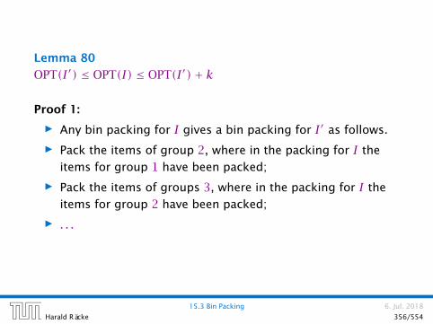
Lemma 80
OPT(I′) ≤ OPT(I) ≤ OPT(I′)+ k
Proof 1:
ñ Any bin packing for I gives a bin packing for I′ as follows.
ñ Pack the items of group 2, where in the packing for I the
items for group 1 have been packed;
ñ Pack the items of groups 3, where in the packing for I the
items for group 2 have been packed;
ñ . . .
15.3 Bin Packing 6. Jul. 2018
Harald Räcke 356/554

Lemma 81
OPT(I′) ≤ OPT(I) ≤ OPT(I′)+ k
Proof 2:
ñ Any bin packing for I′ gives a bin packing for I as follows.
ñ Pack the items of group 1 into k new bins;
ñ Pack the items of groups 2, where in the packing for I′ the
items for group 2 have been packed;
ñ . . .
15.3 Bin Packing 6. Jul. 2018
Harald Räcke 357/554

Assume that our instance does not contain pieces smaller than
ε/2. Then SIZE(I) ≥ εn/2.
We set k = bεSIZE(I)c.
Then n/k ≤ n/bε2n/2c ≤ 4/ε2 (note that bαc ≥ α/2 for α ≥ 1).
Hence, after grouping we have a constant number of piece sizes
(4/ε2) and at most a constant number (2/ε) can fit into any bin.
We can find an optimal packing for such instances by the
previous Dynamic Programming approach.
ñ cost (for large items) at most
OPT(I′)+ k ≤ OPT(I)+ εSIZE(I) ≤ (1+ ε)OPT(I)
ñ running time O((2εn)
4/ε2).

Can we do better?
In the following we show how to obtain a solution where the
number of bins is only
OPT(I)+O(log2(SIZE(I))) .
Note that this is usually better than a guarantee of
(1+ ε)OPT(I)+ 1 .
15.4 Advanced Rounding for Bin Packing 6. Jul. 2018
Harald Räcke 359/554

Configuration LP
Change of Notation:
ñ Group pieces of identical size.
ñ Let s1 denote the largest size, and let b1 denote the number
of pieces of size s1.
ñ s2 is second largest size and b2 number of pieces of size s2;
ñ . . .ñ sm smallest size and bm number of pieces of size sm.
15.4 Advanced Rounding for Bin Packing 6. Jul. 2018
Harald Räcke 360/554

Configuration LP
A possible packing of a bin can be described by an m-tuple
(t1, . . . , tm), where ti describes the number of pieces of size si.Clearly, ∑
iti · si ≤ 1 .
We call a vector that fulfills the above constraint a configuration.
15.4 Advanced Rounding for Bin Packing 6. Jul. 2018
Harald Räcke 361/554

Configuration LP
Let N be the number of configurations (exponential).
Let T1, . . . , TN be the sequence of all possible configurations (a
configuration Tj has Tji pieces of size si).
min∑Nj=1 xj
s.t. ∀i ∈ 1 . . .m ∑Nj=1 Tjixj ≥ bi
∀j ∈ 1, . . . ,N xj ≥ 0
∀j ∈ 1, . . . ,N xj integral
15.4 Advanced Rounding for Bin Packing 6. Jul. 2018
Harald Räcke 362/554

How to solve this LP?
later...
15.4 Advanced Rounding for Bin Packing 6. Jul. 2018
Harald Räcke 363/554
We can assume that each item has size at least 1/SIZE(I).
15.4 Advanced Rounding for Bin Packing 6. Jul. 2018
Harald Räcke 364/554

Harmonic Grouping
ñ Sort items according to size (monotonically decreasing).
ñ Process items in this order; close the current group if size
of items in the group is at least 2 (or larger). Then open new
group.
ñ I.e., G1 is the smallest cardinality set of largest items s.t.
total size sums up to at least 2. Similarly, for G2, . . . , Gr−1.
ñ Only the size of items in the last group Gr may sum up to
less than 2.
15.4 Advanced Rounding for Bin Packing 6. Jul. 2018
Harald Räcke 365/554

Harmonic Grouping
From the grouping we obtain instance I′ as follows:
ñ Round all items in a group to the size of the largest group
member.
ñ Delete all items from group G1 and Gr .ñ For groups G2, . . . , Gr−1 delete ni −ni−1 items.
ñ Observe that ni ≥ ni−1.
15.4 Advanced Rounding for Bin Packing 6. Jul. 2018
Harald Räcke 366/554

Lemma 82
The number of different sizes in I′ is at most SIZE(I)/2.
ñ Each group that survives (recall that G1 and Gr are deleted)
has total size at least 2.
ñ Hence, the number of surviving groups is at most SIZE(I)/2.
ñ All items in a group have the same size in I′.
15.4 Advanced Rounding for Bin Packing 6. Jul. 2018
Harald Räcke 367/554

Lemma 83
The total size of deleted items is at most O(log(SIZE(I))).
ñ The total size of items in G1 and Gr is at most 6 as a group
has total size at most 3.
ñ Consider a group Gi that has strictly more items than Gi−1.
ñ It discards ni −ni−1 pieces of total size at most
3ni −ni−1
ni≤
ni∑
j=ni−1+1
3j
since the average piece size is only 3/ni.ñ Summing over all i that have ni > ni−1 gives a bound of at
most nr−1∑
j=1
3j≤ O(log(SIZE(I))) .
(note that nr ≤ SIZE(I) since we assume that the size of
each item is at least 1/SIZE(I)).

Algorithm 1 BinPack
1: if SIZE(I) < 10 then
2: pack remaining items greedily
3: Apply harmonic grouping to create instance I′; pack
discarded items in at most O(log(SIZE(I))) bins.
4: Let x be optimal solution to configuration LP
5: Pack bxjc bins in configuration Tj for all j; call the
packed instance I1.
6: Let I2 be remaining pieces from I′
7: Pack I2 via BinPack(I2)
15.4 Advanced Rounding for Bin Packing 6. Jul. 2018
Harald Räcke 369/554
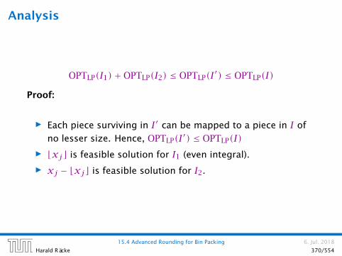
Analysis
OPTLP(I1)+OPTLP(I2) ≤ OPTLP(I′) ≤ OPTLP(I)
Proof:
ñ Each piece surviving in I′ can be mapped to a piece in I of
no lesser size. Hence, OPTLP(I′) ≤ OPTLP(I)ñ bxjc is feasible solution for I1 (even integral).
ñ xj − bxjc is feasible solution for I2.
15.4 Advanced Rounding for Bin Packing 6. Jul. 2018
Harald Räcke 370/554
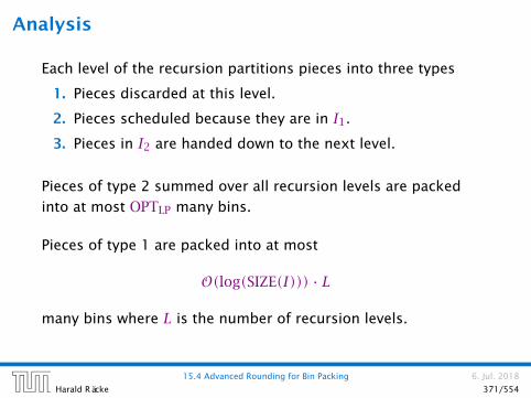
Analysis
Each level of the recursion partitions pieces into three types
1. Pieces discarded at this level.
2. Pieces scheduled because they are in I1.
3. Pieces in I2 are handed down to the next level.
Pieces of type 2 summed over all recursion levels are packed
into at most OPTLP many bins.
Pieces of type 1 are packed into at most
O(log(SIZE(I))) · L
many bins where L is the number of recursion levels.
15.4 Advanced Rounding for Bin Packing 6. Jul. 2018
Harald Räcke 371/554

Analysis
We can show that SIZE(I2) ≤ SIZE(I)/2. Hence, the number of
recursion levels is only O(log(SIZE(Ioriginal))) in total.
ñ The number of non-zero entries in the solution to the
configuration LP for I′ is at most the number of constraints,
which is the number of different sizes (≤ SIZE(I)/2).
ñ The total size of items in I2 can be at most∑Nj=1 xj − bxjc
which is at most the number of non-zero entries in the
solution to the configuration LP.
15.4 Advanced Rounding for Bin Packing 6. Jul. 2018
Harald Räcke 372/554

How to solve the LP?
Let T1, . . . , TN be the sequence of all possible configurations (a
configuration Tj has Tji pieces of size si).In total we have bi pieces of size si.
Primal
min∑Nj=1 xj
s.t. ∀i ∈ 1 . . .m ∑Nj=1 Tjixj ≥ bi
∀j ∈ 1, . . . ,N xj ≥ 0
Dualmax
∑mi=1yibi
s.t. ∀j ∈ 1, . . . ,N ∑mi=1 Tjiyi ≤ 1
∀i ∈ 1, . . . ,m yi ≥ 0
15.4 Advanced Rounding for Bin Packing 6. Jul. 2018
Harald Räcke 373/554

Separation OracleSuppose that I am given variable assignment y for the dual.
How do I find a violated constraint?
I have to find a configuration Tj = (Tj1, . . . , Tjm) that
ñ is feasible, i.e.,m∑
i=1
Tji · si ≤ 1 ,
ñ and has a large profit
m∑
i=1
Tjiyi > 1
But this is the Knapsack problem.
15.4 Advanced Rounding for Bin Packing 6. Jul. 2018
Harald Räcke 374/554

Separation Oracle
We have FPTAS for Knapsack. This means if a constraint is
violated with 1+ ε′ = 1+ ε1−ε we find it, since we can obtain at
least (1− ε) of the optimal profit.
The solution we get is feasible for:
Dual′
max∑mi=1yibi
s.t. ∀j ∈ 1, . . . ,N ∑mi=1 Tjiyi ≤ 1+ ε′
∀i ∈ 1, . . . ,m yi ≥ 0
Primal′
min (1+ ε′)∑Nj=1 xjs.t. ∀i ∈ 1 . . .m ∑N
j=1 Tjixj ≥ bi∀j ∈ 1, . . . ,N xj ≥ 0

Separation OracleIf the value of the computed dual solution (which may be
infeasible) is z then
OPT ≤ z ≤ (1+ ε′)OPT
How do we get good primal solution (not just the value)?
ñ The constraints used when computing z certify that the
solution is feasible for DUAL′.ñ Suppose that we drop all unused constraints in DUAL. We
will compute the same solution feasible for DUAL′.ñ Let DUAL′′ be DUAL without unused constraints.
ñ The dual to DUAL′′ is PRIMAL where we ignore variables for
which the corresponding dual constraint has not been used.
ñ The optimum value for PRIMAL′′ is at most (1+ ε′)OPT.
ñ We can compute the corresponding solution in polytime.

This gives that overall we need at most
(1+ ε′)OPTLP(I)+O(log2(SIZE(I)))
bins.
We can choose ε′ = 1OPT as OPT ≤ #items and since we have a
fully polynomial time approximation scheme (FPTAS) for
knapsack.
15.4 Advanced Rounding for Bin Packing 6. Jul. 2018
Harald Räcke 377/554

Lemma 84 (Chernoff Bounds)
Let X1, . . . , Xn be n independent 0-1 random variables, not
necessarily identically distributed. Then for X =∑ni=1Xi and
µ = E[X], L ≤ µ ≤ U , and δ > 0
Pr[X ≥ (1+ δ)U] <(
eδ
(1+ δ)1+δ)U
,
and
Pr[X ≤ (1− δ)L] <(
e−δ
(1− δ)1−δ)L
,
16.1 Chernoff Bounds 6. Jul. 2018
Harald Räcke 378/554

Lemma 85
For 0 ≤ δ ≤ 1 we have that
(eδ
(1+ δ)1+δ)U≤ e−Uδ2/3
and (e−δ
(1− δ)1−δ)L≤ e−Lδ2/2
16.1 Chernoff Bounds 6. Jul. 2018
Harald Räcke 379/554

Proof of Chernoff Bounds
Markovs Inequality:
Let X be random variable taking non-negative values.
Then
Pr[X ≥ a] ≤ E[X]/a
Trivial!
16.1 Chernoff Bounds 6. Jul. 2018
Harald Räcke 380/554

Proof of Chernoff Bounds
Hence:
Pr[X ≥ (1+ δ)U] ≤ E[X](1+ δ)U ≈
11+ δ
That’s awfully weak :(
16.1 Chernoff Bounds 6. Jul. 2018
Harald Räcke 381/554

Proof of Chernoff Bounds
Set pi = Pr[Xi = 1]. Assume pi > 0 for all i.
Cool Trick:
Pr[X ≥ (1+ δ)U] = Pr[etX ≥ et(1+δ)U]
Now, we apply Markov:
Pr[etX ≥ et(1+δ)U] ≤ E[etX]et(1+δ)U
.
This may be a lot better (!?)
16.1 Chernoff Bounds 6. Jul. 2018
Harald Räcke 382/554

Proof of Chernoff Bounds
E[etX
]= E
[et∑i Xi]= E
[∏i etXi]=∏i E[etXi
]
E[etXi
]= (1− pi)+ piet = 1+ pi(et − 1) ≤ epi(et−1)
∏i E[etXi
]≤∏i epi(et−1) = e
∑pi(et−1) = e(et−1)U
16.1 Chernoff Bounds 6. Jul. 2018
Harald Räcke 383/554

Now, we apply Markov:
Pr[X ≥ (1+ δ)U] = Pr[etX ≥ et(1+δ)U]
≤ E[etX]et(1+δ)U
≤ e(et−1)U
et(1+δ)U≤(
eδ
(1+ δ)1+δ)U
We choose t = ln(1+ δ).
16.1 Chernoff Bounds 6. Jul. 2018
Harald Räcke 384/554

Lemma 86
For 0 ≤ δ ≤ 1 we have that
(eδ
(1+ δ)1+δ)U≤ e−Uδ2/3
and (e−δ
(1− δ)1−δ)L≤ e−Lδ2/2
16.1 Chernoff Bounds 6. Jul. 2018
Harald Räcke 385/554

Show: (eδ
(1+ δ)1+δ)U≤ e−Uδ2/3
Take logarithms:
U(δ− (1+ δ) ln(1+ δ)) ≤ −Uδ2/3
True for δ = 0. Divide by U and take derivatives:
− ln(1+ δ) ≤ −2δ/3
Reason:
As long as derivative of left side is smaller than derivative of
right side the inequality holds.
16.1 Chernoff Bounds 6. Jul. 2018
Harald Räcke 386/554
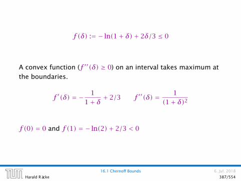
f(δ) := − ln(1+ δ)+ 2δ/3 ≤ 0
A convex function (f ′′(δ) ≥ 0) on an interval takes maximum at
the boundaries.
f ′(δ) = − 11+ δ + 2/3 f ′′(δ) = 1
(1+ δ)2
f(0) = 0 and f(1) = − ln(2)+ 2/3 < 0
16.1 Chernoff Bounds 6. Jul. 2018
Harald Räcke 387/554

For δ ≥ 1 we show(
eδ
(1+ δ)1+δ)U≤ e−Uδ/3
Take logarithms:
U(δ− (1+ δ) ln(1+ δ)) ≤ −Uδ/3
True for δ = 0. Divide by U and take derivatives:
− ln(1+ δ) ≤ −1/3 ⇐⇒ ln(1+ δ) ≥ 1/3 (true)
Reason:
As long as derivative of left side is smaller than derivative of
right side the inequality holds.
16.1 Chernoff Bounds 6. Jul. 2018
Harald Räcke 388/554

Show: (e−δ
(1− δ)1−δ)L≤ e−Lδ2/2
Take logarithms:
L(−δ− (1− δ) ln(1− δ)) ≤ −Lδ2/2
True for δ = 0. Divide by L and take derivatives:
ln(1− δ) ≤ −δ
Reason:
As long as derivative of left side is smaller than derivative of
right side the inequality holds.
16.1 Chernoff Bounds 6. Jul. 2018
Harald Räcke 389/554

ln(1− δ) ≤ −δ
True for δ = 0. Take derivatives:
− 11− δ ≤ −1
This holds for 0 ≤ δ < 1.
16.1 Chernoff Bounds 6. Jul. 2018
Harald Räcke 390/554

Integer Multicommodity Flows
ñ Given si-ti pairs in a graph.
ñ Connect each pair by a path such that not too many path
use any given edge.
min Ws.t. ∀i ∑
p∈Pi xp = 1∑p:e∈p xp ≤ W
xp ∈ 0,1
16.2 Integer Multicommodity Flows 6. Jul. 2018
Harald Räcke 391/554

Integer Multicommodity Flows
Randomized Rounding:
For each i choose one path from the set Pi at random according
to the probability distribution given by the Linear Programming
solution.
16.2 Integer Multicommodity Flows 6. Jul. 2018
Harald Räcke 392/554
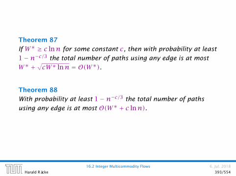
Theorem 87
If W∗ ≥ c lnn for some constant c, then with probability at least
1−n−c/3 the total number of paths using any edge is at most
W∗ +√cW∗ lnn = O(W∗).
Theorem 88
With probability at least 1−n−c/3 the total number of paths
using any edge is at most O(W∗ + c lnn).
16.2 Integer Multicommodity Flows 6. Jul. 2018
Harald Räcke 393/554
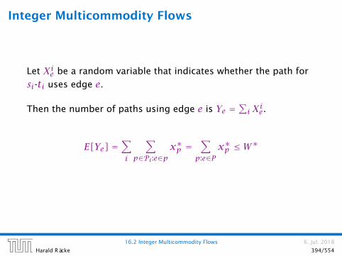
Integer Multicommodity Flows
Let Xie be a random variable that indicates whether the path for
si-ti uses edge e.
Then the number of paths using edge e is Ye =∑iXie.
E[Ye] =∑
i
∑
p∈Pi:e∈px∗p =
∑
p:e∈Px∗p ≤ W∗
16.2 Integer Multicommodity Flows 6. Jul. 2018
Harald Räcke 394/554

Integer Multicommodity Flows
Choose δ = √(c lnn)/W∗.
Then
Pr[Ye ≥ (1+ δ)W∗] < e−W∗δ2/3 = 1nc/3
16.2 Integer Multicommodity Flows 6. Jul. 2018
Harald Räcke 395/554

16.3 MAXSAT
Problem definition:
ñ n Boolean variables
ñ m clauses C1, . . . , Cm. For example
C7 = x3 ∨ x5 ∨ x9
ñ Non-negative weight wj for each clause Cj.ñ Find an assignment of true/false to the variables sucht that
the total weight of clauses that are satisfied is maximum.
16.3 MAXSAT 6. Jul. 2018
Harald Räcke 396/554

16.3 MAXSAT
Terminology:
ñ A variable xi and its negation xi are called literals.
ñ Hence, each clause consists of a set of literals (i.e., no
duplications: xi ∨ xi ∨ xj is not a clause).
ñ We assume a clause does not contain xi and xi for any i.ñ xi is called a positive literal while the negation xi is called a
negative literal.
ñ For a given clause Cj the number of its literals is called its
length or size and denoted with `j.ñ Clauses of length one are called unit clauses.
16.3 MAXSAT 6. Jul. 2018
Harald Räcke 397/554

MAXSAT: Flipping Coins
Set each xi independently to true with probability 12 (and, hence,
to false with probability 12 , as well).
16.3 MAXSAT 6. Jul. 2018
Harald Räcke 398/554

Define random variable Xj with
Xj =
1 if Cj satisfied
0 otw.
Then the total weight W of satisfied clauses is given by
W =∑
jwjXj
16.3 MAXSAT 6. Jul. 2018
Harald Räcke 399/554

E[W] =∑
jwjE[Xj]
=∑
jwjPr[Cj is satisified]
=∑
jwj(1−
(12
)`j)
≥ 12
∑
jwj
≥ 12
OPT
16.3 MAXSAT 6. Jul. 2018
Harald Räcke 400/554

MAXSAT: LP formulation
ñ Let for a clause Cj, Pj be the set of positive literals and Njthe set of negative literals.
Cj =∨
i∈Pjxi ∨
∨
i∈Njxi
max∑jwjzj
s.t. ∀j ∑i∈Pj yi +
∑i∈Nj(1−yi) ≥ zj
∀i yi ∈ 0,1∀j zj ≤ 1
16.3 MAXSAT 6. Jul. 2018
Harald Räcke 401/554
MAXSAT: Randomized Rounding
Set each xi independently to true with probability yi (and,
hence, to false with probability (1−yi)).
16.3 MAXSAT 6. Jul. 2018
Harald Räcke 402/554

Lemma 89 (Geometric Mean ≤ Arithmetic Mean)
For any nonnegative a1, . . . , akk∏
i=1
ai
1/k
≤ 1k
k∑
i=1
ai
16.3 MAXSAT 6. Jul. 2018
Harald Räcke 403/554

Definition 90
A function f on an interval I is concave if for any two points sand r from I and any λ ∈ [0,1] we have
f(λs + (1− λ)r) ≥ λf(s)+ (1− λ)f(r)
Lemma 91
Let f be a concave function on the interval [0,1], with f(0) = aand f(1) = a+ b. Then
f(λ) = f((1− λ)0+ λ1)
≥ (1− λ)f(0)+ λf(1)= a+ λb
for λ ∈ [0,1].
16.3 MAXSAT 6. Jul. 2018
Harald Räcke 404/554

Pr[Cj not satisfied] =∏
i∈Pj(1−yi)
∏
i∈Njyi
≤ 1`j
∑
i∈Pj(1−yi)+
∑
i∈Njyi
`j
=1− 1
`j
∑
i∈Pjyi +
∑
i∈Nj(1−yi)
`j
≤(
1− zj`j
)`j.
16.3 MAXSAT 6. Jul. 2018
Harald Räcke 405/554

The function f(z) = 1− (1− z` )` is concave. Hence,
Pr[Cj satisfied] ≥ 1−(
1− zj`j
)`j
≥1−
(1− 1
`j
)`j · zj .
f ′′(z) = −`−1`
[1− z
`
]`−2 ≤ 0 for z ∈ [0,1]. Therefore, f is
concave.
16.3 MAXSAT 6. Jul. 2018
Harald Räcke 406/554

E[W] =∑
jwjPr[Cj is satisfied]
≥∑
jwjzj
1−
(1− 1
`j
)`j
≥(
1− 1e
)OPT .
16.3 MAXSAT 6. Jul. 2018
Harald Räcke 407/554

MAXSAT: The better of two
Theorem 92
Choosing the better of the two solutions given by randomized
rounding and coin flipping yields a 34 -approximation.
16.3 MAXSAT 6. Jul. 2018
Harald Räcke 408/554

Let W1 be the value of randomized rounding and W2 the value
obtained by coin flipping.
E[maxW1,W2]≥ E[1
2W1 + 12W2]
≥ 12
∑
jwjzj
1−
(1− 1
`j
)`j+ 1
2
∑
jwj
(1−
(12
)`j)
≥∑
jwjzj
1
2
1−
(1− 1
`j
)`j+ 1
2
(1−
(12
)`j)
︸ ︷︷ ︸≥ 3
4 for all integers
≥ 34
OPT
16.3 MAXSAT 6. Jul. 2018
Harald Räcke 409/554

1 2 3 4 5 6
0.5
0.6
0.7
0.8
0.9
1
`
f(`)
randomized rounding
flipping coinsaverage
16.3 MAXSAT 6. Jul. 2018
Harald Räcke 410/554

MAXSAT: Nonlinear Randomized Rounding
So far we used linear randomized rounding, i.e., the probability
that a variable is set to 1/true was exactly the value of the
corresponding variable in the linear program.
We could define a function f : [0,1]→ [0,1] and set xi to true
with probability f(yi).
16.3 MAXSAT 6. Jul. 2018
Harald Räcke 411/554

MAXSAT: Nonlinear Randomized Rounding
Let f : [0,1]→ [0,1] be a function with
1− 4−x ≤ f(x) ≤ 4x−1
Theorem 93
Rounding the LP-solution with a function f of the above form
gives a 34 -approximation.
16.3 MAXSAT 6. Jul. 2018
Harald Räcke 412/554

0 0.5 1
0.5
1
4x−1
1− 4−x
16.3 MAXSAT 6. Jul. 2018
Harald Räcke 413/554

Pr[Cj not satisfied] =∏
i∈Pj(1− f(yi))
∏
i∈Njf(yi)
≤∏
i∈Pj4−yi
∏
i∈Nj4yi−1
= 4−(∑i∈Pj yi+
∑i∈Nj (1−yi))
≤ 4−zj
16.3 MAXSAT 6. Jul. 2018
Harald Räcke 414/554

The function g(z) = 1− 4−z is concave on [0,1]. Hence,
Pr[Cj satisfied] ≥ 1− 4−zj ≥ 34zj .
Therefore,
E[W] =∑
jwjPr[Cj satisfied] ≥ 3
4
∑
jwjzj ≥ 3
4OPT
16.3 MAXSAT 6. Jul. 2018
Harald Räcke 415/554

Can we do better?
Not if we compare ourselves to the value of an optimum
LP-solution.
Definition 94 (Integrality Gap)
The integrality gap for an ILP is the worst-case ratio over all
instances of the problem of the value of an optimal IP-solution to
the value of an optimal solution to its linear programming
relaxation.
Note that the integrality is less than one for maximization
problems and larger than one for minimization problems (of
course, equality is possible).
Note that an integrality gap only holds for one specific ILP
formulation.

Lemma 95
Our ILP-formulation for the MAXSAT problem has integrality gap
at most 34 .
max∑jwjzj
s.t. ∀j ∑i∈Pj yi +
∑i∈Nj(1−yi) ≥ zj
∀i yi ∈ 0,1∀j zj ≤ 1
Consider: (x1 ∨ x2)∧ (x1 ∨ x2)∧ (x1 ∨ x2)∧ (x1 ∨ x2)
ñ any solution can satisfy at most 3 clauses
ñ we can set y1 = y2 = 1/2 in the LP; this allows to set
z1 = z2 = z3 = z4 = 1
ñ hence, the LP has value 4.
16.3 MAXSAT 6. Jul. 2018
Harald Räcke 417/554

MaxCut
MaxCut
Given a weighted graph G = (V , E,w), w(v) ≥ 0, partition the
vertices into two parts. Maximize the weight of edges between
the parts.
Trivial 2-approximation
16.4 MAXCUT 6. Jul. 2018
Harald Räcke 418/554

Semidefinite Programming
max /min∑i,j cijxij
s.t. ∀k ∑i,j,k aijkxij = bk
∀i, j xij = xjiX = (xij) is psd.
ñ linear objective, linear contraints
ñ we can constrain a square matrix of variables to be
symmetric positive definite
Note that wlog. we can assume that all variables appear in this matrix. Supposewe have a non-negative scalar z and want to express something like∑
ij aijkxij + z = bkwhere xij are variables of the positive semidefinite matrix. We can add z as adiagonal entry x``, and additionally introduce constraints x`r = 0 and xr` = 0.
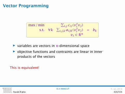
Vector Programming
max /min∑i,j cij(vtivj)
s.t. ∀k ∑i,j,k aijk(vtivj) = bk
vi ∈ Rn
ñ variables are vectors in n-dimensional space
ñ objective functions and contraints are linear in inner
products of the vectors
This is equivalent!
16.4 MAXCUT 6. Jul. 2018
Harald Räcke 420/554
Fact [without proof]
We (essentially) can solve Semidefinite Programs in polynomial
time...
16.4 MAXCUT 6. Jul. 2018
Harald Räcke 421/554

Quadratic Programs
Quadratic Program for MaxCut:
max 12
∑i,jwij(1−yiyj)
∀i yi ∈ −1,1
This is exactly MaxCut!
16.4 MAXCUT 6. Jul. 2018
Harald Räcke 422/554

Semidefinite Relaxation
max 12
∑i,jwij(1− vtivj)
∀i vtivi = 1
∀i vi ∈ Rn
ñ this is clearly a relaxation
ñ the solution will be vectors on the unit sphere
16.4 MAXCUT 6. Jul. 2018
Harald Räcke 423/554

Rounding the SDP-Solution
ñ Choose a random vector r such that r/‖r‖ is uniformly
distributed on the unit sphere.
ñ If r tvi > 0 set yi = 1 else set yi = −1
16.4 MAXCUT 6. Jul. 2018
Harald Räcke 424/554

Rounding the SDP-Solution
Choose the i-th coordinate ri as a Gaussian with mean 0 and
variance 1, i.e., ri ∼N (0,1).
Density function:
ϕ(x) = 1√2πex
2/2
Then
Pr[r = (x1, . . . , xn)]
= 1(√2π
)n ex21/2 · ex2
2/2 · . . . · ex2n/2 dx1 · . . . · dxn
= 1(√2π
)n e12 (x
21+...+x2
n) dx1 · . . . · dxn
Hence the probability for a point only depends on its distance to
the origin.

Rounding the SDP-Solution
Fact
The projection of r onto two unit vectors e1 and e2 are
independent and are normally distributed with mean 0 and
variance 1 iff e1 and e2 are orthogonal.
Note that this is clear if e1 and e2 are standard basis vectors.
16.4 MAXCUT 6. Jul. 2018
Harald Räcke 426/554

Rounding the SDP-Solution
Corollary
If we project r onto a hyperplane its normalized projection
(r ′/‖r ′‖) is uniformly distributed on the unit circle within the
hyperplane.
16.4 MAXCUT 6. Jul. 2018
Harald Räcke 427/554
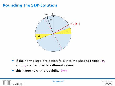
Rounding the SDP-Solution
vivj
r ′/‖r ′‖θ
θ
θ
ñ if the normalized projection falls into the shaded region, viand vj are rounded to different values
ñ this happens with probability θ/π
16.4 MAXCUT 6. Jul. 2018
Harald Räcke 428/554

Rounding the SDP-Solution
ñ contribution of edge (i, j) to the SDP-relaxation:
12wij
(1− vtivj
)
ñ (expected) contribution of edge (i, j) to the rounded
instance wij arccos(vtivj)/πñ ratio is at most
minx∈[−1,1]
2 arccos(x)π(1− x) ≥ 0.878
16.4 MAXCUT 6. Jul. 2018
Harald Räcke 429/554

Rounding the SDP-Solution
−1 −0.5 0 0.5 10
0.25
0.5
0.75
11π arccos(x)12 (1− x)
16.4 MAXCUT 6. Jul. 2018
Harald Räcke 430/554

Rounding the SDP-Solution
−1 −0.5 0 0.5 100
0.5
1
1.5
2
ratio(x)0.878
16.4 MAXCUT 6. Jul. 2018
Harald Räcke 431/554
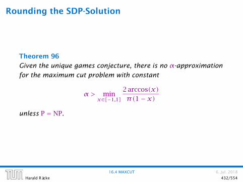
Rounding the SDP-Solution
Theorem 96
Given the unique games conjecture, there is no α-approximation
for the maximum cut problem with constant
α > minx∈[−1,1]
2 arccos(x)π(1− x)
unless P = NP.
16.4 MAXCUT 6. Jul. 2018
Harald Räcke 432/554
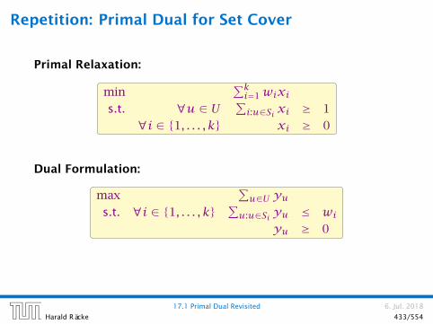
Repetition: Primal Dual for Set Cover
Primal Relaxation:
min∑ki=1wixi
s.t. ∀u ∈ U ∑i:u∈Si xi ≥ 1
∀i ∈ 1, . . . , k xi ≥ 0
Dual Formulation:
max∑u∈U yu
s.t. ∀i ∈ 1, . . . , k ∑u:u∈Si yu ≤ wi
yu ≥ 0
17.1 Primal Dual Revisited 6. Jul. 2018
Harald Räcke 433/554

Repetition: Primal Dual for Set Cover
Algorithm:
ñ Start with y = 0 (feasible dual solution).
Start with x = 0 (integral primal solution that may be
infeasible).
ñ While x not feasibleñ Identify an element e that is not covered in current primal
integral solution.ñ Increase dual variable ye until a dual constraint becomes
tight (maybe increase by 0!).ñ If this is the constraint for set Sj set xj = 1 (add this set to
your solution).
17.1 Primal Dual Revisited 6. Jul. 2018
Harald Räcke 434/554

Repetition: Primal Dual for Set Cover
Analysis:
ñ For every set Sj with xj = 1 we have
∑
e∈Sjye = wj
ñ Hence our cost is∑
jwjxj =
∑
j
∑
e∈Sjye =
∑e|j : e ∈ Sj| ·ye
≤ f ·∑eye ≤ f ·OPT
17.1 Primal Dual Revisited 6. Jul. 2018
Harald Räcke 435/554

Note that the constructed pair of primal and dual solution fulfills
primal slackness conditions.
This means
xj > 0⇒∑
e∈Sjye = wj
If we would also fulfill dual slackness conditions
ye > 0⇒∑
j:e∈Sjxj = 1
then the solution would be optimal!!!
17.1 Primal Dual Revisited 6. Jul. 2018
Harald Räcke 436/554

We don’t fulfill these constraint but we fulfill an approximate
version:
ye > 0⇒ 1 ≤∑
j:e∈Sjxj ≤ f
This is sufficient to show that the solution is an
f -approximation.
17.1 Primal Dual Revisited 6. Jul. 2018
Harald Räcke 437/554

Suppose we have a primal/dual pair
min∑j cjxj
s.t. ∀i ∑j: aijxj ≥ bi
∀j xj ≥ 0
max∑i biyi
s.t. ∀j ∑i aijyi ≤ cj
∀i yi ≥ 0
and solutions that fulfill approximate slackness conditions:
xj > 0⇒∑
iaijyi ≥ 1
αcj
yi > 0⇒∑
jaijxj ≤ βbi
17.1 Primal Dual Revisited 6. Jul. 2018
Harald Räcke 438/554

Then
∑
jcjxj ≤ α
∑
j
∑
iaijyi
xj
= α∑
i
∑
jaijxj
yi
≤ αβ ·∑
ibiyi
∑
jcjxjcj
primal cost
right hand side of j-thdual constraint
∑
ibiyi
dual objective
17.1 Primal Dual Revisited 6. Jul. 2018
Harald Räcke 439/554

Feedback Vertex Set for Undirected Graphs
ñ Given a graph G = (V , E) and non-negative weights wv ≥ 0
for vertex v ∈ V .
ñ Choose a minimum cost subset of vertices s.t. every cycle
contains at least one vertex.
17.2 Feedback Vertex Set for Undirected Graphs 6. Jul. 2018
Harald Räcke 440/554

We can encode this as an instance of Set Cover
ñ Each vertex can be viewed as a set that contains some
cycles.
ñ However, this encoding gives a Set Cover instance of
non-polynomial size.
ñ The O(logn)-approximation for Set Cover does not help us
to get a good solution.
17.2 Feedback Vertex Set for Undirected Graphs 6. Jul. 2018
Harald Räcke 441/554

Let C denote the set of all cycles (where a cycle is identified by
its set of vertices)
Primal Relaxation:
min∑v wvxv
s.t. ∀C ∈ C∑v∈C xv ≥ 1
∀v xv ≥ 0
Dual Formulation:
max∑C∈CyC
s.t. ∀v ∈ V ∑C :v∈C yC ≤ wv
∀C yC ≥ 0
17.2 Feedback Vertex Set for Undirected Graphs 6. Jul. 2018
Harald Räcke 442/554

If we perform the previous dual technique for Set Cover we get
the following:
ñ Start with x = 0 and y = 0
ñ While there is a cycle C that is not covered (does not containa chosen vertex).ñ Increase yC until dual constraint for some vertex v
becomes tight.ñ set xv = 1.
17.2 Feedback Vertex Set for Undirected Graphs 6. Jul. 2018
Harald Räcke 443/554

Then∑vwvxv =
∑v
∑
C :v∈CyCxv
=∑
v∈S
∑
C :v∈CyC
=∑
C|S ∩ C| ·yC
where S is the set of vertices we choose.
If every cycle is short we get a good approximation ratio, but
this is unrealistic.
17.2 Feedback Vertex Set for Undirected Graphs 6. Jul. 2018
Harald Räcke 444/554

Algorithm 1 FeedbackVertexSet1: y ← 0
2: x ← 0
3: while exists cycle C in G do
4: increase yC until there is v ∈ C s.t.∑C :v∈C yC = wv
5: xv = 1
6: remove v from G7: repeatedly remove vertices of degree 1 from G
17.2 Feedback Vertex Set for Undirected Graphs 6. Jul. 2018
Harald Räcke 445/554

Idea:
Always choose a short cycle that is not covered. If we always find
a cycle of length at most α we get an α-approximation.
Observation:
For any path P of vertices of degree 2 in G the algorithm
chooses at most one vertex from P .
17.2 Feedback Vertex Set for Undirected Graphs 6. Jul. 2018
Harald Räcke 446/554

Observation:
If we always choose a cycle for which the number of vertices of
degree at least 3 is at most α we get a 2α-approximation.
Theorem 97
In any graph with no vertices of degree 1, there always exists a
cycle that has at most O(logn) vertices of degree 3 or more. We
can find such a cycle in linear time.
This means we have
yC > 0⇒ |S ∩ C| ≤ O(logn) .
17.2 Feedback Vertex Set for Undirected Graphs 6. Jul. 2018
Harald Räcke 447/554
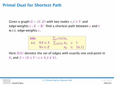
Primal Dual for Shortest Path
Given a graph G = (V , E) with two nodes s, t ∈ V and
edge-weights c : E → R+ find a shortest path between s and tw.r.t. edge-weights c.
min∑e c(e)xe
s.t. ∀S ∈ S ∑e:δ(S) xe ≥ 1
∀e ∈ E xe ∈ 0,1Here δ(S) denotes the set of edges with exactly one end-point in
S, and S = S ⊆ V : s ∈ S, t ∉ S.
17.3 Primal Dual for Shortest Path 6. Jul. 2018
Harald Räcke 448/554

Primal Dual for Shortest Path
The Dual:
max∑S yS
s.t. ∀e ∈ E ∑S:e∈δ(S)yS ≤ c(e)
∀S ∈ S yS ≥ 0
Here δ(S) denotes the set of edges with exactly one end-point in
S, and S = S ⊆ V : s ∈ S, t ∉ S.
17.3 Primal Dual for Shortest Path 6. Jul. 2018
Harald Räcke 449/554
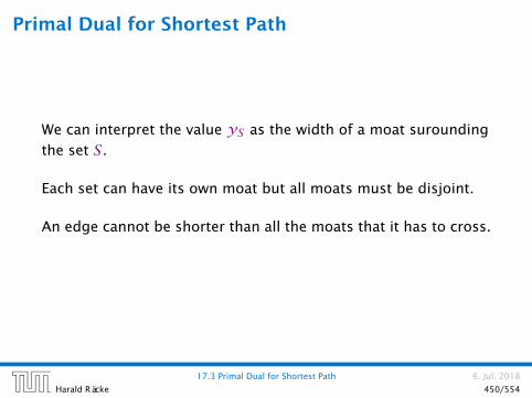
Primal Dual for Shortest Path
We can interpret the value yS as the width of a moat surounding
the set S.
Each set can have its own moat but all moats must be disjoint.
An edge cannot be shorter than all the moats that it has to cross.
17.3 Primal Dual for Shortest Path 6. Jul. 2018
Harald Räcke 450/554

Algorithm 1 PrimalDualShortestPath1: y ← 0
2: F ← 3: while there is no s-t path in (V , F) do
4: Let C be the connected component of (V , F) con-
taining s5: Increase yC until there is an edge e′ ∈ δ(C) such
that∑S:e′∈δ(S)yS = c(e′).
6: F ← F ∪ e′7: Let P be an s-t path in (V , F)8: return P
17.3 Primal Dual for Shortest Path 6. Jul. 2018
Harald Räcke 451/554

Lemma 98
At each point in time the set F forms a tree.
Proof:
ñ In each iteration we take the current connected component
from (V , F) that contains s (call this component C) and add
some edge from δ(C) to F .
ñ Since, at most one end-point of the new edge is in C the
edge cannot close a cycle.
17.3 Primal Dual for Shortest Path 6. Jul. 2018
Harald Räcke 452/554
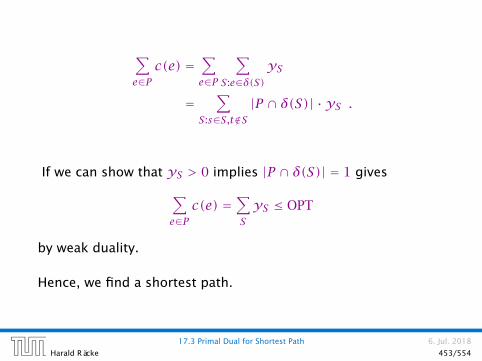
∑
e∈Pc(e) =
∑
e∈P
∑
S:e∈δ(S)yS
=∑
S:s∈S,t∉S|P ∩ δ(S)| ·yS .
If we can show that yS > 0 implies |P ∩ δ(S)| = 1 gives
∑
e∈Pc(e) =
∑
SyS ≤ OPT
by weak duality.
Hence, we find a shortest path.
17.3 Primal Dual for Shortest Path 6. Jul. 2018
Harald Räcke 453/554

If S contains two edges from P then there must exist a subpath
P ′ of P that starts and ends with a vertex from S (and all interior
vertices are not in S).
When we increased yS , S was a connected component of the set
of edges F ′ that we had chosen till this point.
F ′ ∪ P ′ contains a cycle. Hence, also the final set of edges
contains a cycle.
This is a contradiction.
17.3 Primal Dual for Shortest Path 6. Jul. 2018
Harald Räcke 454/554

Steiner Forest Problem:
Given a graph G = (V , E), together with source-target pairs si, ti,i = 1, . . . , k, and a cost function c : E → R+ on the edges. Find a
subset F ⊆ E of the edges such that for every i ∈ 1, . . . , k there
is a path between si and ti only using edges in F .
min∑e c(e)xe
s.t. ∀S ⊆ V : S ∈ Si for some i∑e∈δ(S) xe ≥ 1
∀e ∈ E xe ∈ 0,1
Here Si contains all sets S such that si ∈ S and ti ∉ S.
17.4 Steiner Forest 6. Jul. 2018
Harald Räcke 455/554

max∑S : ∃i s.t. S ∈ Si yS
s.t. ∀e ∈ E ∑S:e∈δ(S)yS ≤ c(e)
yS ≥ 0
The difference to the dual of the shortest path problem is that
we have many more variables (sets for which we can generate a
moat of non-zero width).
17.4 Steiner Forest 6. Jul. 2018
Harald Räcke 456/554

Algorithm 1 FirstTry1: y ← 0
2: F ← 3: while not all si-ti pairs connected in F do
4: Let C be some connected component of (V , F)such that |C ∩ si, ti| = 1 for some i.
5: Increase yC until there is an edge e′ ∈ δ(C) s.t.∑S∈Si:e′∈δ(S)yS = ce′
6: F ← F ∪ e′7: return
⋃i Pi
17.4 Steiner Forest 6. Jul. 2018
Harald Räcke 457/554

∑
e∈Fc(e) =
∑
e∈F
∑
S:e∈δ(S)yS =
∑
S|δ(S)∩ F| ·yS .
If we show that yS > 0 implies that |δ(S)∩ F| ≤ α we are in
good shape.
However, this is not true:
ñ Take a complete graph on k+ 1 vertices v0, v1, . . . , vk.ñ The i-th pair is v0-vi.ñ The first component C could be v0.ñ We only set yv0 = 1. All other dual variables stay 0.
ñ The final set F contains all edges v0, vi, i = 1, . . . , k.
ñ yv0 > 0 but |δ(v0)∩ F| = k.
17.4 Steiner Forest 6. Jul. 2018
Harald Räcke 458/554

Algorithm 1 SecondTry
1: y ← 0; F ← ; ` ← 0
2: while not all si-ti pairs connected in F do
3: ` ← ` + 1
4: Let C be set of all connected components C of (V , F)such that |C ∩ si, ti| = 1 for some i.
5: Increase yC for all C ∈ C uniformly until for some edge
e` ∈ δ(C′), C′ ∈ C s.t.∑S:e`∈δ(S)yS = ce`
6: F ← F ∪ e`7: F ′ ← F8: for k← ` downto 1 do // reverse deletion
9: if F ′ − ek is feasible solution then
10: remove ek from F ′
11: return F ′
17.4 Steiner Forest 6. Jul. 2018
Harald Räcke 459/554

The reverse deletion step is not strictly necessary this way. It
would also be sufficient to simply delete all unnecessary edges
in any order.
17.4 Steiner Forest 6. Jul. 2018
Harald Räcke 460/554

Example
s1 s2
s3
t1
t2
t3
17.4 Steiner Forest 6. Jul. 2018
Harald Räcke 461/554

Lemma 99
For any C in any iteration of the algorithm
∑
C∈C
|δ(C)∩ F ′| ≤ 2|C|
This means that the number of times a moat from C is crossed in
the final solution is at most twice the number of moats.
Proof: later...
17.4 Steiner Forest 6. Jul. 2018
Harald Räcke 462/554

∑
e∈F ′ce =
∑
e∈F ′
∑
S:e∈δ(S)yS =
∑
S|F ′ ∩ δ(S)| ·yS .
We want to show that
∑
S|F ′ ∩ δ(S)| ·yS ≤ 2
∑
SyS
ñ In the i-th iteration the increase of the left-hand side is
ε∑
C∈C
|F ′ ∩ δ(C)|
and the increase of the right hand side is 2ε|C|.ñ Hence, by the previous lemma the inequality holds after the
iteration if it holds in the beginning of the iteration.
17.4 Steiner Forest 6. Jul. 2018
Harald Räcke 463/554

Lemma 100
For any set of connected components C in any iteration of the
algorithm ∑
C∈C
|δ(C)∩ F ′| ≤ 2|C|
Proof:
ñ At any point during the algorithm the set of edges forms a
forest (why?).
ñ Fix iteration i. Let Fi be the set of edges in F at the
beginning of the iteration.
ñ Let H = F ′ − Fi.ñ All edges in H are necessary for the solution.
17.4 Steiner Forest 6. Jul. 2018
Harald Räcke 464/554

ñ Contract all edges in Fi into single vertices V ′.
ñ We can consider the forest H on the set of vertices V ′.
ñ Let deg(v) be the degree of a vertex v ∈ V ′ within this forest.
ñ Color a vertex v ∈ V ′ red if it corresponds to a component fromC (an active component). Otw. color it blue. (Let B the set of bluevertices (with non-zero degree) and R the set of red vertices)
ñ We have
∑
v∈Rdeg(v) ≥
∑
C∈C
|δ(C)∩ F ′| ?≤ 2|C| = 2|R|
17.4 Steiner Forest 6. Jul. 2018
Harald Räcke 465/554

ñ Suppose that no node in B has degree one.
ñ Then∑
v∈Rdeg(v) =
∑
v∈R∪Bdeg(v)−
∑
v∈Bdeg(v)
≤ 2(|R| + |B|)− 2|B| = 2|R|
ñ Every blue vertex with non-zero degree must have degree atleast two.ñ Suppose not. The single edge connecting b ∈ B comes fromH, and, hence, is necessary.
ñ But this means that the cluster corresponding to b mustseparate a source-target pair.
ñ But then it must be a red node.
17.4 Steiner Forest 6. Jul. 2018
Harald Räcke 466/554
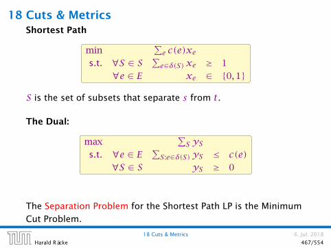
18 Cuts & MetricsShortest Path
min∑e c(e)xe
s.t. ∀S ∈ S ∑e∈δ(S) xe ≥ 1
∀e ∈ E xe ∈ 0,1
S is the set of subsets that separate s from t.
The Dual:
max∑S yS
s.t. ∀e ∈ E ∑S:e∈δ(S)yS ≤ c(e)
∀S ∈ S yS ≥ 0
The Separation Problem for the Shortest Path LP is the Minimum
Cut Problem.
18 Cuts & Metrics 6. Jul. 2018
Harald Räcke 467/554

18 Cuts & MetricsMinimum Cut
min∑e c(e)xe
s.t. ∀P ∈ P ∑e∈P xe ≥ 1
∀e ∈ E xe ∈ 0,1
P is the set of path that connect s and t.
The Dual:
max∑P yP
s.t. ∀e ∈ E ∑P :e∈P yP ≤ c(e)
∀P ∈ P yP ≥ 0
The Separation Problem for the Minimum Cut LP is the Shortest
Path Problem.
18 Cuts & Metrics 6. Jul. 2018
Harald Räcke 468/554

18 Cuts & Metrics
Observations:
Suppose that `e-values are solution to Minimum Cut LP.
ñ We can view `e as defining the length of an edge.
ñ Define d(u,v) =minpath P btw. u and v∑e∈P `e as the
Shortest Path Metric induced by `e.ñ We have d(u,v) = `e for every edge e = (u,v), as otw. we
could reduce `e without affecting the distance between sand t.
Remark for bean-counters:
d is not a metric on V but a semimetric as two nodes u and vcould have distance zero.
18 Cuts & Metrics 6. Jul. 2018
Harald Räcke 469/554

How do we round the LP?
ñ Let B(s, r) be the ball of radius r around s (w.r.t. metric d).
Formally:
B = v ∈ V | d(s, v) ≤ r
ñ For 0 ≤ r < 1, B(s, r) is an s-t-cut.
Which value of r should we choose? choose randomly!!!
Formally:
choose r u.a.r. (uniformly at random) from interval [0,1)
18 Cuts & Metrics 6. Jul. 2018
Harald Räcke 470/554

What is the probability that an edge (u, v) is in the cut?
s u
v
t
ñ asssume wlog. d(s,u) ≤ d(s, v)
Pr[e is cut] = Pr[r ∈ [d(s,u),d(s, v))] ≤ d(s, v)− d(s,u)1− 0
≤ `e
18 Cuts & Metrics 6. Jul. 2018
Harald Räcke 471/554

What is the expected size of a cut?
E[size of cut] = E[∑
e c(e)Pr[e is cut]]
≤∑e c(e)`e
On the other hand:
∑e c(e)`e ≤ size of mincut
as the `e are the solution to the Mincut LP relaxation.
Hence, our rounding gives an optimal solution.
18 Cuts & Metrics 6. Jul. 2018
Harald Räcke 472/554

Minimum Multicut:
Given a graph G = (V , E), together with source-target pairs si, ti,i = 1, . . . , k, and a capacity function c : E → R+ on the edges.
Find a subset F ⊆ E of the edges such that all si-ti pairs lie in
different components in G = (V , E \ F).
min∑e c(e)`e
s.t. ∀P ∈ Pi for some i∑e∈P `e ≥ 1
∀e ∈ E `e ∈ 0,1
Here Pi contains all path P between si and ti.
18 Cuts & Metrics 6. Jul. 2018
Harald Räcke 473/554

Re-using the analysis for the single-commodity case is
difficult.
Pr[e is cut] ≤ ?
ñ If for some R the balls B(si, R) are disjoint between different
sources, we get a 1/R approximation.
ñ However, this cannot be guaranteed.
18 Cuts & Metrics 6. Jul. 2018
Harald Räcke 474/554

ñ Assume for simplicity that all edge-length `e are multiples
of δ 1.
ñ Replace the graph G by a graph G′, where an edge of length
`e is replaced by `e/δ edges of length δ.
ñ Let B(si, z) be the ball in G′ that contains nodes v with
distance d(si, v) ≤ zδ.
Algorithm 1 RegionGrowing(si, p)1: z ← 0
2: repeat
3: flip a coin (Pr[heads] = p)
4: z ← z + 1
5: until heads
6: return B(si, z)
18 Cuts & Metrics 6. Jul. 2018
Harald Räcke 475/554

Algorithm 1 Multicut(G′)1: while ∃si-ti pair in G′ do
2: C ← RegionGrowing(si, p)3: G′ = G′ \ C // cuts edges leaving C4: return B(si, z)
ñ probability of cutting an edge is only pñ a source either does not reach an edge during Region
Growing; then it is not cut
ñ if it reaches the edge then it either cuts the edge or protects
the edge from being cut by other sources
ñ if we choose p = δ the probability of cutting an edge is only
its LP-value; our expected cost are at most OPT.
18 Cuts & Metrics 6. Jul. 2018
Harald Räcke 476/554

Problem:
We may not cut all source-target pairs.
A component that we remove may contain an si-ti pair.
If we ensure that we cut before reaching radius 1/2 we are in
good shape.
18 Cuts & Metrics 6. Jul. 2018
Harald Räcke 477/554

ñ choose p = 6 lnk · δñ we make 1
2δ trials before reaching radius 1/2.
ñ we say a Region Growing is not successful if it does not
terminate before reaching radius 1/2.
Pr[not successful] ≤ (1−p) 12δ =
((1−p)1/p
) p2δ ≤ e− p
2δ ≤ 1k3
ñ Hence,
Pr[∃i that is not successful] ≤ 1k2
18 Cuts & Metrics 6. Jul. 2018
Harald Räcke 478/554

What is expected cost?
E[cutsize] = Pr[success] · E[cutsize | success]
+ Pr[no success] · E[cutsize | no success]
E[cutsize | succ.] = E[cutsize]− Pr[no succ.] · E[cutsize | no succ.]Pr[success]
≤ E[cutsize]Pr[success]
≤ 1
1− 1k2
6 lnk ·OPT ≤ 8 lnk ·OPT
Note: success means all source-target pairs separated
We assume k ≥ 2.
18 Cuts & Metrics 6. Jul. 2018
Harald Räcke 479/554

If we are not successful we simply perform a trivial
k-approximation.
This only increases the expected cost by at most1k2 · kOPT ≤ OPT/k.
Hence, our final cost is O(lnk) ·OPT in expectation.
18 Cuts & Metrics 6. Jul. 2018
Harald Räcke 480/554

Gap Introducing Reduction
yes
no
value ≤ n
value > 2n
gap
HAM TSP
Reduction from Hamiltonian cycle to TSP
ñ instance that has Hamiltonian cycle is mapped to TSP
instance with small cost
ñ otherwise it is mapped to instance with large cost
ñ =⇒ there is no 2n/n-approximation for TSP

PCP theorem: Approximation View
Theorem 101 (PCP Theorem A)
There exists ε > 0 for which there is gap introducing reduction
between 3SAT and MAX3SAT.
yes
no
1
≤ 1− ε
gap
3SAT MAX3SAT
Here the goal of the MAX3SAT-problem is tomaximize the fraction of satisfied clauses. Theabove theorem implies that we cannot approxi-mate MAX3SAT with a ratio better than 1− ε.
The standard formula-tion of the PCP theo-rem looks very differ-ent but the above theo-rem is equivalent. Orig-inally, the PCP theoremis a result about interac-tive proof systems andits importance to hard-ness of approximationis somewhat a side ef-fect.

PCP theorem: Proof System View
Definition 102 (NP)
A language L ∈ NP if there exists a polynomial time,
deterministic verifier V (a Turing machine), s.t.
[x ∈ L] completeness
There exists a proof string y, |y| = poly(|x|),s.t. V(x,y) = “accept”.
[x ∉ L] soundness
For any proof string y, V(x,y) = “reject”.
Note that requiring |y| = poly(|x|) for x ∉ L does not make a
difference (why?).
19 Hardness of Approximation 6. Jul. 2018
Harald Räcke 483/554

Probabilistic Checkable Proofs
An Oracle Turing Machine M is a Turing machine that has access
to an oracle.
Such an oracle allows M to solve some problem in a single step.
For example having access to a TSP-oracle πTSP would allow Mto write a TSP-instance x on a special oracle tape and obtain the
answer (yes or no) in a single step.
For such TMs one looks in addition to running time also at query
complexity, i.e., how often the machine queries the oracle.
For a proof string y, πy is an oracle that upon given an index ireturns the i-th character yi of y.
19 Hardness of Approximation 6. Jul. 2018
Harald Räcke 484/554

Probabilistic Checkable Proofs
Definition 103 (PCP)
A language L ∈ PCPc(n),s(n)(r(n), q(n)) if there exists a
polynomial time, non-adaptive, randomized verifier V , s.t.
[x ∈ L] There exists a proof string y, s.t. Vπy (x) = “ac-
cept” with probability ≥ c(n).
[x ∉ L] For any proof string y, Vπy (x) = “accept” with
probability ≤ s(n).
The verifier uses at most O(r(n)) random bits and makes at
most O(q(n)) oracle queries.
Note that the proof itself does not count towards the input of the verifier. The verifier has to writethe number of a bit-position it wants to read onto a special tape, and then the correspondingbit from the proof is returned to the verifier. The proof may only be exponentially long, as apolynomial time verifier cannot address longer proofs.
Non-adaptive means that e.g. the sec-ond proof-bit read by the verifier maynot depend on the value of the first bit.

Probabilistic Checkable Proofs
c(n) is called the completeness. If not specified otw. c(n) = 1.
Probability of accepting a correct proof.
s(n) < c(n) is called the soundness. If not specified otw.
s(n) = 1/2. Probability of accepting a wrong proof.
r(n) is called the randomness complexity, i.e., how many
random bits the (randomized) verifier uses.
q(n) is the query complexity of the verifier.
19 Hardness of Approximation 6. Jul. 2018
Harald Räcke 486/554

Probabilistic Checkable Proofs
ñ P = PCP(0,0)verifier without randomness and proof access is
deterministic algorithm
ñ PCP(logn,0) ⊆ P
we can simulate O(logn) random bits in deterministic,
polynomial time
ñ PCP(0, logn) ⊆ P
we can simulate short proofs in polynomial time
ñ PCP(poly(n),0) = coRP?!= P
by definition; coRP is randomized polytime with one sided
error (positive probability of accepting NO-instance)
Note that the first three statements also hold with equality
RP = coRP = P is a commonly believedconjecture. RP stands for randomizedpolynomial time (with a non-zero prob-ability of rejecting a YES-instance).
19 Hardness of Approximation 6. Jul. 2018
Harald Räcke 487/554

Probabilistic Checkable Proofs
ñ PCP(0,poly(n)) = NP
by definition; NP-verifier does not use randomness and asks
polynomially many queries
ñ PCP(logn,poly(n)) ⊆ NP
NP-verifier can simulate O(logn) random bits
ñ PCP(poly(n),0) = coRP?!⊆ NP
ñ NP ⊆ PCP(logn,1)hard part of the PCP-theorem
19 Hardness of Approximation 6. Jul. 2018
Harald Räcke 488/554

PCP theorem: Proof System View
Theorem 104 (PCP Theorem B)
NP = PCP(logn,1)
19 Hardness of Approximation 6. Jul. 2018
Harald Räcke 489/554

Probabilistic Proof for Graph NonIsomorphism
GNI is the language of pairs of non-isomorphic graphs
Verifier gets input (G0, G1) (two graphs with n-nodes)
It expects a proof of the following form:
ñ For any labeled n-node graph H the H’s bit P[H] of the
proof fulfills
G0 ≡ H =⇒ P[H] = 0
G1 ≡ H =⇒ P[H] = 1
G0, G1 H =⇒ P[H] = arbitrary
19 Hardness of Approximation 6. Jul. 2018
Harald Räcke 490/554

Probabilistic Proof for Graph NonIsomorphism
Verifier:
ñ choose b ∈ 0,1 at random
ñ take graph Gb and apply a random permutation to obtain a
labeled graph Hñ check whether P[H] = b
If G0 G1 then by using the obvious proof the verifier will
always accept.
If G0 ≡ G1 a proof only accepts with probability 1/2.
ñ suppose π(G0) = G1
ñ if we accept for b = 1 and permutation πrand we reject for
b = 0 and permutation πrand π
19 Hardness of Approximation 6. Jul. 2018
Harald Räcke 491/554

Version B =⇒ Version A
ñ For 3SAT there exists a verifier that uses c logn random
bits, reads q = O(1) bits from the proof, has completeness
1 and soundness 1/2.
ñ fix x and r :
input
x, rproof bits
πj1 , . . . , πjq
computation
fx,r (πj1 , . . . , πjq)
reject accept
0 1
19 Hardness of Approximation 6. Jul. 2018
Harald Räcke 492/554

Version B =⇒ Version A
ñ transform Boolean formula fx,r into 3SAT formula Cx,r(constant size, variables are proof bits)
ñ consider 3SAT formula Cx Í∧r Cx,r
[x ∈ L] There exists proof string y, s.t. all formulas Cx,revaluate to 1. Hence, all clauses in Cx satisfied.
[x ∉ L] For any proof string y, at most 50% of formulas
Cx,r evaluate to 1. Since each contains only a
constant number of clauses, a constant fraction
of clauses in Cx are not satisfied.
ñ this means we have gap introducing reduction
19 Hardness of Approximation 6. Jul. 2018
Harald Räcke 493/554

Version A =⇒ Version B
We show: Version A =⇒ NP ⊆ PCP1,1−ε(logn,1).
given L ∈ NP we build a PCP-verifier for L
Verifier:
ñ 3SAT is NP-complete; map instance x for L into 3SAT
instance Ix, s.t. Ix satisfiable iff x ∈ Lñ map Ix to MAX3SAT instance Cx (PCP Thm. Version A)
ñ interpret proof as assignment to variables in Cxñ choose random clause X from Cxñ query variable assignment σ for X;
ñ accept if X(σ) = true otw. reject

Version A =⇒ Version B
[x ∈ L] There exists proof string y, s.t. all clauses in Cxevaluate to 1. In this case the verifier returns 1.
[x ∉ L] For any proof string y, at most a (1−ε)-fraction
of clauses in Cx evaluate to 1. The verifier will
reject with probability at least ε.
To show Theorem B we only need to run this verifier a constant
number of times to push rejection probability above 1/2.
19 Hardness of Approximation 6. Jul. 2018
Harald Räcke 495/554

NP ⊆ PCP(poly(n), 1)
PCP(poly(n),1) means we have a potentially exponentially long
proof but we only read a constant number of bits from it.
The idea is to encode an NP-witness (e.g. a satisfying assignment
(say n bits)) by a code whose code-words have 2n bits.
A wrong proof is either
ñ a code-word whose pre-image does not correspond to a
satisfying assignment
ñ or, a sequence of bits that does not correspond to a
code-word
We can detect both cases by querying a few positions.
Note that this approach has strong con-nections to error correction codes.
19 Hardness of Approximation 6. Jul. 2018
Harald Räcke 496/554

The Code
u ∈ 0,1n (satisfying assignment)
Walsh-Hadamard Code:
WHu : 0,1n → 0,1, x , xTu (over GF(2))
The code-word for u is WHu. We identify this function by a
bit-vector of length 2n.
19 Hardness of Approximation 6. Jul. 2018
Harald Räcke 497/554

The Code
Lemma 105
If u ≠ u′ then WHu and WHu′ differ in at least 2n−1 bits.
Proof:
Suppose that u−u′ ≠ 0. Then
WHu(x) ≠ WHu′(x)⇐⇒ (u−u′)Tx ≠ 0
This holds for 2n−1 different vectors x.
19 Hardness of Approximation 6. Jul. 2018
Harald Räcke 498/554

The Code
Suppose we are given access to a function f : 0,1n → 0,1and want to check whether it is a codeword.
Since the set of codewords is the set of all linear functions
0,1n to 0,1 we can check
f(x +y) = f(x)+ f(y)
for all 22n pairs x,y. But that’s not very efficient.
19 Hardness of Approximation 6. Jul. 2018
Harald Räcke 499/554
NP ⊆ PCP(poly(n), 1)
Can we just check a constant number of positions?
19 Hardness of Approximation 6. Jul. 2018
Harald Räcke 500/554

NP ⊆ PCP(poly(n), 1)
Definition 106
Let ρ ∈ [0,1]. We say that f , g : 0,1n → 0,1 are ρ-close if
Prx∈0,1n
[f (x) = g(x)] ≥ ρ .
Theorem 107 (proof deferred)
Let f : 0,1n → 0,1 with
Prx,y∈0,1n
[f(x)+ f(y) = f(x +y)
]≥ ρ > 1
2.
Then there is a linear function f such that f and f are ρ-close.
Observe that for two codewordsPrx∈0,1n[f (x) = g(x)] = 1/2.
19 Hardness of Approximation 6. Jul. 2018
Harald Räcke 501/554

NP ⊆ PCP(poly(n), 1)
We need O(1/δ) trials to be sure that f is (1− δ)-close to a
linear function with (arbitrary) constant probability.
19 Hardness of Approximation 6. Jul. 2018
Harald Räcke 502/554

NP ⊆ PCP(poly(n), 1)
Suppose for δ < 1/4 f is (1− δ)-close to some linear function f .
f is uniquely defined by f , since linear functions differ on at
least half their inputs.
Suppose we are given x ∈ 0,1n and access to f . Can we
compute f (x) using only constant number of queries?
19 Hardness of Approximation 6. Jul. 2018
Harald Räcke 503/554

NP ⊆ PCP(poly(n), 1)
Suppose we are given x ∈ 0,1n and access to f . Can we
compute f (x) using only constant number of queries?
1. Choose x′ ∈ 0,1n u.a.r.
2. Set x′′ := x + x′.3. Let y′ = f(x′) and y′′ = f(x′′).4. Output y′ +y′′.
x′ and x′′ are uniformly distributed (albeit dependent). With
probability at least 1− 2δ we have f(x′) = f (x′) and
f(x′′) = f (x′′).
Then the above routine returns f (x).
This technique is known as local decoding of the
Walsh-Hadamard code.

NP ⊆ PCP(poly(n), 1)
We show that QUADEQ ∈ PCP(poly(n),1). The theorem follows
since any PCP-class is closed under polynomial time reductions.
QUADEQ
Given a system of quadratic equations over GF(2). Is there a
solution?
19 Hardness of Approximation 6. Jul. 2018
Harald Räcke 505/554

QUADEQ is NP-complete
ñ given 3SAT instance C represent it as Boolean circuit
e.g. C = (x1 ∨ x2 ∨ x3)∧ (x3 ∨ x4 ∨ x5)∧ (x6 ∨ x7 ∨ x8)ñ add variable for every wire
ñ add constraint for every gate
OR: i1 + i2 + i1 · i2 = oAND: i1 · i2 = oNEG: i = 1− o
ñ add constraint out = 1
ñ system is feasible iff
C is satisfiable
x1 x2 x3 x4 x5 x6 x7 x8
a hb
out
c
de
f
go
i2i1
d · e = g
19 Hardness of Approximation 6. Jul. 2018
Harald Räcke 506/554

NP ⊆ PCP(poly(n), 1)
We encode an instance of QUADEQ by a matrix A that has n2
columns; one for every pair i, j; and a right hand side vector b.
For an n-dimensional vector x we use x ⊗ x to denote the
n2-dimensional vector whose i, j-th entry is xixj.
Then we are asked whether
A(x ⊗ x) = b
has a solution.
Note that over GF(2) x = x2. Therefore,we can assume that there are no termsof degree 1.

NP ⊆ PCP(poly(n), 1)
Let A, b be an instance of QUADEQ. Let u be a satisfying
assignment.
The correct PCP-proof will be the Walsh-Hadamard encodings of
u and u⊗u. The verifier will accept such a proof with
probability 1.
We have to make sure that we reject proofs that do not
correspond to codewords for vectors of the form u, and u⊗u.
We also have to reject proofs that correspond to codewords for
vectors of the form z, and z ⊗ z, where z is not a satisfying
assignment.
19 Hardness of Approximation 6. Jul. 2018
Harald Räcke 508/554

NP ⊆ PCP(poly(n), 1)
Step 1. Linearity Test.
The proof contains 2n + 2n2
bits. This is interpreted as a pair of
functions f : 0,1n → 0,1 and g : 0,1n2 → 0,1.
We do a 0.999-linearity test for both functions (requires a
constant number of queries).
We also assume that for the remaining constant number of
accesses WH-decoding succeeds and we recover f (x).
Hence, our proof will only ever see f . To simplify notation we
use f for f , in the following (similar for g, g).
Recall that for a correct proof there is nodifference between f and f .

NP ⊆ PCP(poly(n), 1)
We need to show that the probability of accepting a wrong proof is small.This first step means that in order to fool us with reasonable probability a wrong proof
needs to be very close to a linear function. The probability that we accept a proof when thefunctions are not close to linear is just a small constant.
Similarly, if the functions are close to linear then the probability that the Walsh Hadamarddecoding fails (for any of the remaining accesses) is just a small constant. If we ignore thissmall constant error then a malicious prover could also provide a linear function (as a nearlinear function f is “rounded” by us to the corresponding linear function f ). If this rounding issuccessful it doesn’t make sense for the prover to provide a function that is not linear.
19 Hardness of Approximation 6. Jul. 2018
Harald Räcke 510/554

NP ⊆ PCP(poly(n), 1)
Step 2. Verify that g encodes u ⊗ u where u is string
encoded by f .
f(r) = uTr and g(z) = wTz since f , g are linear.
ñ choose r , r ′ independently, u.a.r. from 0,1nñ if f(r)f (r ′) ≠ g(r ⊗ r ′) reject
ñ repeat 3 times
19 Hardness of Approximation 6. Jul. 2018
Harald Räcke 511/554

NP ⊆ PCP(poly(n), 1)
A correct proof survives the test
f(r) · f(r ′) = uTr ·uTr ′
=(∑
iuiri
)·(∑
jujr ′j
)
=∑
ijuiujrir ′j
= (u⊗u)T (r ⊗ r ′)= g(r ⊗ r ′)
19 Hardness of Approximation 6. Jul. 2018
Harald Räcke 512/554

NP ⊆ PCP(poly(n), 1)
Suppose that the proof is not correct and w ≠ u⊗u.
Let W be n×n-matrix with entries from w. Let U be matrix with
Uij = ui ·uj (entries from u⊗u).
g(r ⊗ r ′) = wT (r ⊗ r ′) =∑
ijwijrir ′j = rTWr ′
f(r)f (r ′) = uTr ·uTr ′ = rTUr ′
If U ≠ W then Wr ′ ≠ Ur ′ with probability at least 1/2. Then
rTWr ′ ≠ rTUr ′ with probability at least 1/4.
For a non-zero vector x and a random vector r (both with elements fromGF(2)), we have Pr[xT r ≠ 0] = 1
2 . This holds because the product is zero iffthe number of ones in r that “hit” ones in x in the product is even.

NP ⊆ PCP(poly(n), 1)
Step 3. Verify that f encodes satisfying assignment.
We need to check
Ak(u⊗u) = bkwhere Ak is the k-th row of the constraint matrix. But the left
hand side is just g(ATk ).
We can handle this by a single query but checking all constraints
would take O(m) steps.
We compute rTA, where r ∈R 0,1m. If u is not a satisfying
assignment then with probability 1/2 the vector r will hit an odd
number of violated constraints.
In this case rTA(u⊗u) ≠ rTbk. The left hand side is equal to
g(ATr).

NP ⊆ PCP(poly(n), 1)
We used the following theorem for the linearity test:
Theorem 107
Let f : 0,1n → 0,1 with
Prx,y∈0,1n
[f(x)+ f(y) = f(x +y)
]≥ ρ > 1
2.
Then there is a linear function f such that f and f are ρ-close.
19 Hardness of Approximation 6. Jul. 2018
Harald Räcke 515/554

NP ⊆ PCP(poly(n), 1)
Fourier Transform over GF(2)
In the following we use −1,1 instead of 0,1. We map
b ∈ 0,1 to (−1)b.
This turns summation into multiplication.
The set of function f : −1,1n → R form a 2n-dimensional
Hilbert space.
19 Hardness of Approximation 6. Jul. 2018
Harald Räcke 516/554

NP ⊆ PCP(poly(n), 1)
Hilbert space
ñ addition (f + g)(x) = f(x)+ g(x)ñ scalar multiplication (αf)(x) = αf(x)ñ inner product 〈f , g〉 = Ex∈−1,1n[f (x)g(x)]
(bilinear, 〈f , f 〉 ≥ 0, and 〈f , f 〉 = 0⇒ f = 0)
ñ completeness: any sequence xk of vectors for which
∞∑
k=1
‖xk‖ <∞ fulfills
∥∥∥∥∥∥L−N∑
k=1
xk
∥∥∥∥∥∥→ 0
for some vector L.
19 Hardness of Approximation 6. Jul. 2018
Harald Räcke 517/554

NP ⊆ PCP(poly(n), 1)
standard basis
ex(y) =
1 x = y0 otw.
Then, f(x) =∑iαiei(x) where αx = f(x), this means the
functions ei form a basis. This basis is orthonormal.
19 Hardness of Approximation 6. Jul. 2018
Harald Räcke 518/554

NP ⊆ PCP(poly(n), 1)
fourier basis
For α ⊆ [n] define
χα(x) =∏
i∈αxi
Note that
〈χα, χβ〉 = Ex[χα(x)χβ(x)
]= Ex
[χα4β(x)
]=
1 α = β0 otw.
This means the χα’s also define an orthonormal basis. (since we
have 2n orthonormal vectors...)
19 Hardness of Approximation 6. Jul. 2018
Harald Räcke 519/554

NP ⊆ PCP(poly(n), 1)
A function χα multiplies a set of xi’s. Back in the GF(2)-world
this means summing a set of zi’s where xi = (−1)zi .
This means the function χα correspond to linear functions in the
GF(2) world.
19 Hardness of Approximation 6. Jul. 2018
Harald Räcke 520/554

NP ⊆ PCP(poly(n), 1)
We can write any function f : −1,1n → R as
f =∑αfαχα
We call fα the αth Fourier coefficient.
Lemma 108
1. 〈f , g〉 =∑α fαgα2. 〈f , f 〉 =∑α f 2
α
Note that for Boolean functions f : −1,1n → −1,1,〈f , f 〉 = 1.
〈f , f 〉 = Ex[f (x)2] = 1
19 Hardness of Approximation 6. Jul. 2018
Harald Räcke 521/554

Linearity Test
in GF(2):We want to show that if Prx,y[f (x)+ f(y) = f(x +y)] is large
than f has a large agreement with a linear function.
in Hilbert space: (we will prove)
Suppose f : ±1n → −1,1 fulfills
Prx,y[f (x)f(y) = f(x y)] ≥ 1
2+ ε .
Then there is some α ⊆ [n], s.t. fα ≥ 2ε.
Here x y denotes the n-dimensional vector with entryxiyi in position i (Hadamard product).Observe that we have χα(x y) = χα(x)χα(y).
19 Hardness of Approximation 6. Jul. 2018
Harald Räcke 522/554

Linearity Test
For Boolean functions 〈f , g〉 is the fraction of inputs on which
f , g agree minus the fraction of inputs on which they disagree.
2ε ≤ fα = 〈f , χα〉 = agree− disagree = 2agree− 1
This gives that the agreement between f and χα is at least 12 +ε.
19 Hardness of Approximation 6. Jul. 2018
Harald Räcke 523/554

Linearity Test
Prx,y[f (x y) = f(x)f(y)] ≥ 1
2+ ε
means that the fraction of inputs x,y on which f(x y) and
f(x)f(y) agree is at least 1/2+ ε.
This gives
Ex,y[f (x y)f(x)f(y)] = agreement− disagreement
= 2agreement− 1
≥ 2ε
19 Hardness of Approximation 6. Jul. 2018
Harald Räcke 524/554
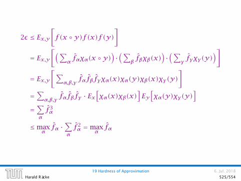
2ε ≤ Ex,y[f(x y)f(x)f(y)
]
= Ex,y[(∑
α fαχα(x y))·(∑
β fβχβ(x))·(∑
γ fγχγ(y))]
= Ex,y[∑
α,β,γ fαfβfγχα(x)χα(y)χβ(x)χγ(y)]
=∑α,β,γ fαfβfγ · Ex
[χα(x)χβ(x)
]Ey[χα(y)χγ(y)
]
=∑αf 3α
≤maxαfα ·
∑αf 2α =max
αfα
19 Hardness of Approximation 6. Jul. 2018
Harald Räcke 525/554

Approximation Preserving Reductions
AP-reduction
ñ x ∈ I1 ⇒ f(x, r) ∈ I2ñ SOL1(x) ≠ ⇒ SOL2(f (x, r)) ≠ ñ y ∈ SOL2(f (x, r)) ⇒ g(x,y, r) ∈ SOL2(x)ñ f ,g are polynomial time computable
ñ R2(f (x, r),y) ≤ r ⇒ R1(x, g(x,y, r)) ≤ 1+α(r − 1)
19 Hardness of Approximation 6. Jul. 2018
Harald Räcke 526/554
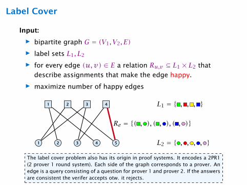
Label Cover
Input:
ñ bipartite graph G = (V1, V2, E)ñ label sets L1, L2
ñ for every edge (u,v) ∈ E a relation Ru,v ⊆ L1 × L2 that
describe assignments that make the edge happy.
ñ maximize number of happy edges
1 2 3 4
1 2 3 4 5
L1 = , , ,
L2 = , , , ,
Re = ( , ), ( , ), ( , )
The label cover problem also has its origin in proof systems. It encodes a 2PR1(2 prover 1 round system). Each side of the graph corresponds to a prover. Anedge is a query consisting of a question for prover 1 and prover 2. If the answersare consistent the verifer accepts otw. it rejects.
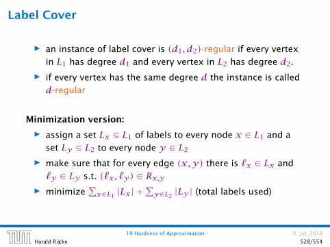
Label Cover
ñ an instance of label cover is (d1, d2)-regular if every vertex
in L1 has degree d1 and every vertex in L2 has degree d2.
ñ if every vertex has the same degree d the instance is called
d-regular
Minimization version:
ñ assign a set Lx ⊆ L1 of labels to every node x ∈ L1 and a
set Ly ⊆ L2 to every node y ∈ L2
ñ make sure that for every edge (x,y) there is `x ∈ Lx and
`y ∈ Ly s.t. (`x, `y) ∈ Rx,yñ minimize
∑x∈L1 |Lx| +
∑y∈L2 |Ly | (total labels used)
19 Hardness of Approximation 6. Jul. 2018
Harald Räcke 528/554

MAX E3SAT via Label Cover
instance:
Φ(x) = (x1 ∨ x2 ∨ x3)∧ (x4 ∨ x2 ∨ x3)∧ (x1 ∨ x2 ∨ x4)
corresponding graph:
x1 x2 x3 x4
x1 ∨ x2 ∨ x3 x4 ∨ x2 ∨ x3 x1 ∨ x2 ∨ x4
label sets: L1 = T , F3, L2 = T , F (T=true, F=false)
relation: RC,xi = ((ui, uj , uk),ui), where the clause C is over
variables xi, xj , xk and assignment (ui, uj , uk) satisfies C
R = ((F, F, F), F), ((F, T , F), F), ((F, F, T), T), ((F, T , T), T),((T , T , T), T), ((T , T , F), F), ((T , F, F), F)
The verifier accepts if the la-belling (assignment to vari-ables in clauses at the top+ assignment to variables atthe bottom) causes the clauseto evaluate to true and is con-sistent, i.e., the assignmentof e.g. x4 at the bottom isthe same as the assignmentgiven to x4 in the labelling ofthe clause.

MAX E3SAT via Label Cover
Lemma 109
If we can satisfy k out of m clauses in φ we can make at least
3k+ 2(m− k) edges happy.
Proof:
ñ for V2 use the setting of the assignment that satisfies kclauses
ñ for satisfied clauses in V1 use the corresponding
assignment to the clause-variables (gives 3k happy edges)
ñ for unsatisfied clauses flip assignment of one of the
variables; this makes one incident edge unhappy (gives
2(m− k) happy edges)
19 Hardness of Approximation 6. Jul. 2018
Harald Räcke 530/554

MAX E3SAT via Label Cover
Lemma 110
If we can satisfy at most k clauses in Φ we can make at most
3k+ 2(m− k) = 2m+ k edges happy.
Proof:
ñ the labeling of nodes in V2 gives an assignment
ñ every unsatisfied clause in this assignment cannot be
assigned a label that satisfies all 3 incident edges
ñ hence at most 3m− (m− k) = 2m+ k edges are happy
19 Hardness of Approximation 6. Jul. 2018
Harald Räcke 531/554

Hardness for Label Cover
We cannot distinguish between the following two cases
ñ all 3m edges can be made happy
ñ at most 2m+ (1− ε)m = (3− ε)m out of the 3m edges can
be made happy
Hence, we cannot obtain an approximation constant α > 3−ε3 .
Here ε > 0 is the constant from PCP The-orem A.
19 Hardness of Approximation 6. Jul. 2018
Harald Räcke 532/554

(3, 5)-regular instances
Theorem 111
There is a constant ρ s.t. MAXE3SAT is hard to approximate with
a factor of ρ even if restricted to instances where a variable
appears in exactly 5 clauses.
Then our reduction has the following properties:
ñ the resulting Label Cover instance is (3,5)-regular
ñ it is hard to approximate for a constant α < 1
ñ given a label `1 for x there is at most one label `2 for ythat makes edge (x,y) happy (uniqueness property)
19 Hardness of Approximation 6. Jul. 2018
Harald Räcke 533/554

(3, 5)-regular instances
The previous theorem can be obtained with a series of
gap-preserving reductions:
ñ MAX3SAT ≤ MAX3SAT(≤ 29)ñ MAX3SAT(≤ 29) ≤ MAX3SAT(≤ 5)ñ MAX3SAT(≤ 5) ≤ MAX3SAT(= 5)ñ MAX3SAT(= 5) ≤ MAXE3SAT(= 5)
Here MAX3SAT(≤ 29) is the variant of MAX3SAT in which a
variable appears in at most 29 clauses. Similar for the other
problems.
19 Hardness of Approximation 6. Jul. 2018
Harald Räcke 534/554

Regular instances
Theorem 112
There is a constant α < 1 such if there is an α-approximation
algorithm for Label Cover on 15-regular instances than P=NP.
Given a label `1 for x ∈ V1 there is at most one label `2 for ythat makes (x,y) happy. (uniqueness property)
We take the (3,5)-regular instance. We make 3 copies ofevery clause vertex and 5 copies of every variable vertex.Then we add edges between clause vertex and variablevertex iff the clause contains the variable. This increasesthe size by a constant factor. The gap instance can stilleither only satisfy a constant fraction of the edges or alledges. The uniqueness property still holds for the newinstance.
19 Hardness of Approximation 6. Jul. 2018
Harald Räcke 535/554

Parallel Repetition
We would like to increase the inapproximability for Label Cover.
In the verifier view, in order to decrease the acceptance
probability of a wrong proof (or as here: a pair of wrong proofs)
one could repeat the verification several times.
Unfortunately, we have a 2P1R-system, i.e., we are stuck with a
single round and cannot simply repeat.
The idea is to use parallel repetition, i.e., we simply play several
rounds in parallel and hope that the acceptance probability of
wrong proofs goes down.
19 Hardness of Approximation 6. Jul. 2018
Harald Räcke 536/554

Parallel Repetition
Given Label Cover instance I with G = (V1, V2, E), label sets L1
and L2 we construct a new instance I′:
ñ V ′1 = Vk1 = V1 × · · · × V1
ñ V ′2 = Vk2 = V2 × · · · × V2
ñ L′1 = Lk1 = L1 × · · · × L1
ñ L′2 = Lk2 = L2 × · · · × L2
ñ E′ = Ek = E × · · · × EAn edge ((x1, . . . , xk), (y1, . . . , yk)) whose end-points are
labelled by (`x1 , . . . , `xk ) and (`y1 , . . . , `
yk ) is happy if
(`xi , `yi ) ∈ Rxi,yi for all i.
19 Hardness of Approximation 6. Jul. 2018
Harald Räcke 537/554

Parallel Repetition
If I is regular than also I′.
If I has the uniqueness property than also I′.
Did the gap increase?
ñ Suppose we have labelling `1, `2 that satisfies just an
α-fraction of edges in I.ñ We transfer this labelling to instance I′:
vertex (x1, . . . , xk) gets label (`1(x1), . . . , `1(xk)),vertex (y1, . . . , yk) gets label (`2(y1), . . . , `2(yk)).
ñ How many edges are happy?
only (α|E|)k out of |E|k!!! (just an αk fraction)
Does this always work?
19 Hardness of Approximation 6. Jul. 2018
Harald Räcke 538/554

Counter Example
Non interactive agreement:
ñ Two provers A and Bñ The verifier generates two random bits bA, and bB, and
sends one to A and one to B.
ñ Each prover has to answer one of A0, A1, B0, B1 with the
meaning A0 := prover A has been given a bit with value 0.
ñ The provers win if they give the same answer and if the
answer is correct.
19 Hardness of Approximation 6. Jul. 2018
Harald Räcke 539/554

Counter Example
The provers can win with probability at most 1/2.
0
1
0
1
0
1
0
1
A B
A0 A1
A1
Regardless what we do 50% of edges are unhappy!
19 Hardness of Approximation 6. Jul. 2018
Harald Räcke 540/554

Counter Example
In the repeated game the provers can
also win with probability 1/2:
0,0
0,1
1,0
1,1
0,0
1,0
0,1
1,1
0,0
0,1
1,0
1,1
0,0
1,0
0,1
1,1
A B
A0, B0
A0, B0
A0, B0
A0, B0
A1, B1
A1, B1
A1, B1
A1, B1
For the first game/coordinate theprovers give an answer of the form“A has received...” (A0 or A1) andfor the second an answer of theform “B has received...” (B0 or B1).
If the answer a prover has togive is about himself a prover cananswer correctly. If the answer tobe given is about the other proverthe same bit is returned. Thismeans e.g. Prover B answers A1
for the first game iff in the secondgame he receives a 1-bit.
By this method the provers al-ways win if Prover A gets the samebit in the first game as Prover B inthe second game. This happenswith probability 1/2.
This strategy is not possible forthe provers if the game is repeatedsequentially. How should prover Bknow (for her answer in the firstgame) which bit she is going to re-ceive in the second game?
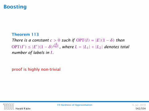
Boosting
Theorem 113
There is a constant c > 0 such if OPT(I) = |E|(1− δ) then
OPT(I′) ≤ |E′|(1− δ)ck
logL , where L = |L1| + |L2| denotes total
number of labels in I.
proof is highly non-trivial
19 Hardness of Approximation 6. Jul. 2018
Harald Räcke 542/554
Hardness of Label Cover
Theorem 114
There are constants c > 0, δ < 1 s.t. for any k we cannot
distinguish regular instances for Label Cover in which either
ñ OPT(I) = |E|, or
ñ OPT(I) = |E|(1− δ)ckunless each problem in NP has an algorithm running in time
O(nO(k)).
Corollary 115
There is no α-approximation for Label Cover for any constant α.
19 Hardness of Approximation 6. Jul. 2018
Harald Räcke 543/554

Hardness of Set Cover
Theorem 116
There exist regular Label Cover instances s.t. we cannot
distinguish whether
ñ all edges are satisfiable, or
ñ at most a 1/ log2(|L1||E|)-fraction is satisfiable
unless NP-problems have algorithms with running time
O(nO(log logn)).
choose k ≥ 2c log1/(1−δ)(log(|L1||E|)) = O(log logn).
19 Hardness of Approximation 6. Jul. 2018
Harald Räcke 544/554

Hardness of Set Cover
Partition System (s, t, h)ñ universe U of size sñ t pairs of sets (A1, A1), . . . , (At , At);Ai ⊆ U, Ai = U \Ai
ñ choosing from any h pairs only one of Ai, Ai we do not
cover the whole set U
we will show later:
for any h, t with h ≤ t there exist systems with s = |U| ≤ 4t22h
19 Hardness of Approximation 6. Jul. 2018
Harald Räcke 545/554

Hardness of Set Cover
Given a Label Cover instance we construct a Set Cover instance;
The universe is E ×U , where U is the universe of some partition
system; (t = |L1|, h = log(|E||L1|))
for all u ∈ V1, `1 ∈ L1
Su,`1= ((u,v),a) | (u,v) ∈ E,a ∈ A`1
for all v ∈ V2, `2 ∈ L2
Sv,`2= ((u,v),a) | (u,v) ∈ E,a ∈ A`1
, where (`1, `2) ∈ R(u,v)
note that Sv,`2is well defined because of uniqueness property
19 Hardness of Approximation 6. Jul. 2018
Harald Räcke 546/554

Hardness of Set Cover
Suppose that we can make all edges happy.
Choose sets Su,`1’s and Sv,`2
’s, where `1 is the label we
assigned to u, and `2 the label for v. (|V1|+|V2| sets)
For an edge (u,v), Sv,`2contains (u,v) ×A`2
. For a happy
edge Su,`1contains (u,v) × A`2
.
Since all edges are happy we have covered the whole universe.
If the Label Cover instance is completely satisfiable we can cover
with |V1| + |V2| sets.
19 Hardness of Approximation 6. Jul. 2018
Harald Räcke 547/554

Hardness of Set Cover
Lemma 117
Given a solution to the set cover instance using at mosth8 (|V1| + |V2|) sets we can find a solution to the Label Cover
instance satisfying at least 2h2 |E| edges.
If the Label Cover instance cannot satisfy a 2/h2-fraction we
cannot cover with h8 (|V1| + |V2|) sets.
Since differentiating between both cases for the Label Cover
instance is hard, we have an O(h)-hardness for Set Cover.
19 Hardness of Approximation 6. Jul. 2018
Harald Räcke 548/554

Hardness of Set Cover
ñ nu: number of Su,i’s in cover
ñ nv : number of Sv,j’s in cover
ñ at most 1/4 of the vertices can have nu, nv ≥ h/2; mark
these vertices
ñ at least half of the edges have both end-points unmarked,
as the graph is regular
ñ for such an edge (u,v) we must have chosen Su,i and a
corresponding Sv,j, s.t. (i, j) ∈ Ru,v (making (u,v) happy)
ñ we choose a random label for u from the (at most h/2)
chosen Su,i-sets and a random label for v from the (at most
h/2) Sv,j-sets
ñ (u,v) gets happy with probability at least 4/h2
ñ hence we make a 2/h2-fraction of edges happy
19 Hardness of Approximation 6. Jul. 2018
Harald Räcke 549/554

Set Cover
Theorem 118
There is no 132 logn-approximation for the unweighted Set Cover
problem unless problems in NP can be solved in time
O(nO(log logn)).
19 Hardness of Approximation 6. Jul. 2018
Harald Räcke 550/554

Given label cover instance (V1, V2, E), label sets L1 and L2;
Set h = log(|E||L1|) and t = |L1|; Size of partition system is
s = |U| = 4t22h = 4|L1|2(|E||L1|)2 = 4|E|2|L1|4
The size of the ground set is then
n = |E||U| = 4|E|3|L2|4 ≤ (|E||L2|)4
for sufficiently large |E|. Then h ≥ 14 logn.
If we get an instance where all edges are satisfiable there exists
a cover of size only |V1| + |V2|.
If we find a cover of size at most h8 (|V1| + |V2|) we can use this
to satisfy at least a fraction of 2/h2 ≥ 1/ log2(|E||L1|) of the
edges. this is not possible...

Partition Systems
Lemma 119
Given h and t with h ≤ t, there is a partition system of size
s = ln(4t)h2h ≤ 4t22h.
We pick t sets at random from the possible 2|U| subsets of U .
Fix a choice of h of these sets, and a choice of h bits (whether
we choose Ai or Ai). There are 2h ·(th
)such choices.
19 Hardness of Approximation 6. Jul. 2018
Harald Räcke 552/554

What is the probability that a given choice covers U?
The probability that an element u ∈ Ai is 1/2 (same for Ai).
The probability that u is covered is 1− 12h
.
The probability that all u are covered is (1− 12h)s
The probability that there exists a choice such that all u are
covered is at most(th
)2h(
1− 12h
)s≤ (2t)he−s/2h = (2t)h · e−h ln(4t) <
12.
The random process outputs a partition system with constant
probability!
19 Hardness of Approximation 6. Jul. 2018
Harald Räcke 553/554

Advanced PCP TheoremHere the verifier reads exactly three bitsfrom the proof. Not O(3) bits.
Theorem 120
For any positive constant ε > 0, it is the case that
NP ⊆ PCP1−ε,1/2+ε(logn,3). Moreover, the verifier just reads
three bits from the proof, and bases its decision only on the
parity of these bits.
It is NP-hard to approximate a MAXE3LIN problem by a factor
better than 1/2+ δ, for any constant δ.
It is NP-hard to approximate MAX3SAT better than 7/8+ δ, for
any constant δ.
19 Hardness of Approximation 6. Jul. 2018
Harald Räcke 554/554