EhmhmhhhmD - apps.dtic.mil

AD-AlOO 439 PENNSYLVANIA STATE UNIV UNIVERSITY PARK DEPT OF METE-ETC F/6 4/2ESTIMATION OF VERTICAL WIND SHEAR FROM INFRARED AND MICROWAVE R-.ETC(U)APR 81 H A PANOPSKY. .J Ji CANIR, A CAVALIER N00OOIASO-C-0115UNCASSUTrn N

~ EhmhmhhhmD

1 LEVE f, PENN STATEI [Estimation of Vertical Wind Shear from

infrared and Microwave Radiances

C/i Hans A. PanofskyAf Jchn J. LCair

Anthony CavalierI Frederick Gadomski

I DEPARTMENT OF METEOROLOGY THE PENNSYLVANIA STATE UNIVERSITY

Final ReportNaval Environmental Prediction Research Facility

Monterey, CA

Contract #' N00014-80-C-0115

[l1981 i '-rl--

81 1- - --4 T

4ECU,',ITY CLASSIFICATION OF THIS PAGE ("ouen Date Entered)

REPORT DOCUMENTATION PAGE BRE TNSTCTORMI. REPORT NUMBER 2. GOVT ACCESSION NO. 3. RECIPIENT'S CATALOG NUMBER

4. TITLE (and Subtitle) S. TYP9 OF RlpORT 6-04RJUO C.OyERED\ .. -- - / Final Rept for period,.&STIMATION OF V RTICAL WIND SHEAR FROM 1 Deco.-I979--30 Avr1.JIN8l

INFRARED AND MICROWAVE RADIANCES Qtt !.N. ORG. REPORT NUMBER

'7.,AUTHR(&)S. CONTRACT OR GRANT NUMBER(#)Hans A./Panofsky?7ohn J. /Cahir,-Anthony/Cavalier Frederick/Gadomski 0014-80-C-0115",

9. PERFORMING ORGANIZATION NAME AND ADDRESS 10. PROGRAM ELEMENT, PROJECT, TASKAREA A WORK UNIT NUMBERS

The Pennsylvania State University 123302Department of Meteorology

I I. CONTROLLING OFFICE NAME AND ADDRESS 12. REPORT DATESAp rl 981 - ... 7Naval Environmental Prediction Research -3. NUMBER OF PAGES

Facility, Monterey, California 65

14. MONITORING AGENCY NAME A ADDRESS(f different from Controfllng Office) IS. SECURITY CLASS. (of this report)

Naval Environmental Prediction Research Unclassified

Facility, Monterey, California .SCHEDULEAIICATION/OOWNGRAOING

IS. DISTRIBUTION STATEMENT (of this Report)

Scientific Officer 1 NRL Code 2627 1ONR Branch Office 1 DDC 2ACO 1 Fiscal Officer NEPRF 3 (shipped separately)

17. DISTRIBUTION STATEMENT (of the abstract entered in Block 20, If different from Report)

NA

IS. SUPPLEMENTARY NOTES

19. KEY WORDS (Continue on reverie side If neceelry and Identify by block number)

Wind shear; radiance gradients; microwave channels; geostrophic wind; clearradiances; satellite radiances; linear radiance combinations

20. AB PRACT (Continue on reverie side If necessary and Identify by block number)

Linear regression estimates of radiosonde observed vertical wind shearsbetween mandatory levels were made, using radiance gradients obtained viathe TIROS-N satellite as predictors in a pilot experiment based on about200-500 observations. The best results were obtained for shears between850 mb and a level in the upper troposphere, such as 300 mb. Results weresimilar for 850-400 or 850-200 mb shears, but notably inferior for850-500 mb shears. The linear correlation coefficients between estimated

DD JAN73 1473 EDITION OF I NOV65 IS OBSOLETES/N 0102.L.014-6601

SECURITY CLASSIFICATION OF THIS PAGE (When Date niered).

....i. ......

SECuRITY CLASSIFICATION OF THIS PAGE ("on Data Entered;

Ijand smoothed observed components of shear was about 0.70, correspondingto about 50 percent explained variance in independent test samples. Some-what higher explained variances (about 0.60) were achieved in a limitedtrial where the data-set was stratified according to subjectively-judgedtrajectory curvature.

Estimates of the wind itself in the upper troposphere were nearlyas skillful as the best shear results. Overall, with the possible excep-tion of curvature-stratified estimates in clear regions, both wind andwind shear estimates are not likely to be superior to methods that generateRMS wind errors of order 5

Most of the information was contributed by the linear combination ofmicrowave channel 2 minus microwave channel 3. Some additional informationmay be obtainable from the infrared (HIRS-2) channels 3, 4 and 5(especially 5).

SECURITY CLASSIFICATION OF-THIS PAGEMloth Date Entered)

!i4

JI

Estimation of Vertical Wind Shear from

Infrared and Microwave Radiances

Final Report to

Director, Atmospheric and Ionospheric Sciences ProgramArctic and Earth Sciences Division

Office of Naval Research

Under Contract # N00014-80-C-0115

Naval Environmental Prediction Research Facility

Monterey, CA

byjHans A. PanofskyJohn J. CahirAnthony Cavalier

Frederick Gadomski

1 The Pennsylvania State UniversityDepartment of Meteorology

Accession '"or

NTIS G?4:.:DTIC TAB

U11al-, lounvedJusti C tir"

April 1981 ~~U_Distribution/

Dist p c al

)A

I I

I4 -ii-

Summary

This project was a pilot study aimed toward testing the hypothesis that

vertical wind shear through the middle troposphere can be usefully estimated

by linear combinations of satellite-sensed infrared and microwave radiance

gradients. Linear regression estimates were made, with observed shears

between mandatory levels as predictands and radiance gradients obtained via

the TIROS-N satellite as predictors. Data observed during March 1979 over

the western United States were used. Radiances were interpolated according

to a neighboring-points slope-fitting analysis scheme to the radiosonde sites;

the mesh-equivalence of the radiance data was about 250 km, so that synoptic

scale radiance gradients were the predictors.

Data problems limited the sample sizes severely. Level lB data,

initially tested, were useless. Level 2A data for March 1979 contained no

1500 LST data, necessary for 0000 GMT comparisons over the western United

States, at all. Further, the retrievals on individual days exhibit many missing

i Idata. Finally, cloudiness seriously limits the available data points for the

infrared. As a result, the pilot experiments are based on about 200-500 obser-

I vations apiece, which limits the confidence one can place in the conclusion.

They must be considered very tentative.

The best results were obtained for shears between 850 mb and a level in

the upper troposphere, such as 300 mb. Results were similar for 850-400 or

1 850-200 mb shears, but notably inferior for 850-500 mb shears.

I The linear correlation coefficients between estimated and smoothed obser-

ved components of shear was about 0.70, corresponding to about 50 percent

explained variance in independent test samples. Somewhat higher explained

45,

~-iii-

variances (about 0.60) were achieved in a limited trial where the data-set

was stratified according to subjectively-judged trajectory curvature.

In developmental trials, regression estimates of the wind itself in

the upper tcoposphere were very similar in skill to the best shear results.

However, these deteriorated somewhat in the independent trial on smoothed

data, presumably oecause the shears contained more random error. Overall,

with the possible exception of curvature-stratified estimates in clear

regions, both wind and wind shear estimates are not likely to be superior to

methods that generate RMS wind errors of order 5 ms-1 .

With respect to predictors, one result was quite consistent: Most of

the information was contributed by the linear combination of microwave chan-

nel 2 minus microwave channel 3. Some additional information may be obtain-

able from the infrared (HIRS-2) channels 3, 4 and 5 (especially 5); indeed,

the highest explained variances, and the best result in the curvature-

stratified experiment involved linear combinations of the five microwave

and infrared channels. Nevertheless, the HIRS channel results were disappoint-

ing. Even with a carefully checked set of clear points relatively free of

interpolation errors, the infrared-only experiments did not match the microwave

only experiments in skill. Part of the reason for this is stratospheric

remperatare gradient reversal, where the tropopause is low. This weakens the

radiance gradients, especially in HIRS channels 3 and 4.

Further experiments are needed, on a much larger sample. Microwave

channels 2 and 3, or microwave plus infrared channel 5 (or 3, 4 and 5) are the

indicated predictors. Equations should be derived on unsmoothed wind shear

observations but tested on smoothed ones. An objective method of stratification

of trajectory curvature should be developed and tested. Finally, a rigorous

I-iv-

test of standard errors of these estimates against those of alternative wind

shear calculations should be made.

4

1

1

I

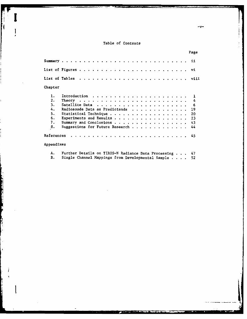
Table of Contents

Page

Summary. .. ..................... .. .. .. ... i

List of Figures .. ........... .............. vi

List of Tables. ........... ............... viii

Chapter

1. Introduction .. .......................2. Theory .. ..................... .... 43. Satellite Data .. ..................... 64. Radiosonde Data as Predictands .. ............. 195. Statistical Technique .. .......... ....... 206. Experiments and Results .. ........... ..... 237. Summary and Conclusions .. .......... ...... 43.8. Suggestions for Future Research. .. ............ 44

References. ........... ................. 45

Appendixes

A. Further Details on TIROS-N Radiance Data Processing . 47

B. Single Channel Mappings from Developmental Sample . . . . 52

-vi-

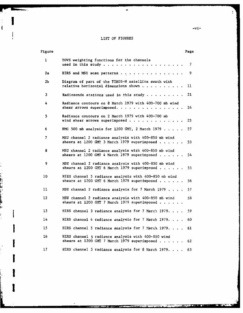
LIST OF FIGURES

Figure Page

1 TOVS weighting functions for the channelsused in this study ......... ................... 7

2a HIRS and MSU scan patterns ....... ............... 9

2b Diagram of part of the TIROS-N satellite swath withrelative horizontal dimensions shown ... .......... . .11

3 Radiosonde stations used in this study ........... ... 21

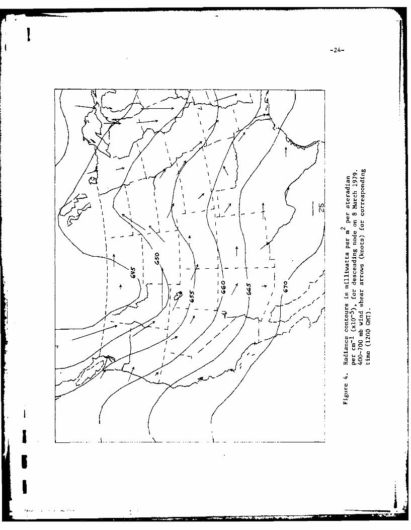
4 Radiance contours on 8 March 1979 with 400-700 mb windshear arrows superimposed ..... ................ ... 24

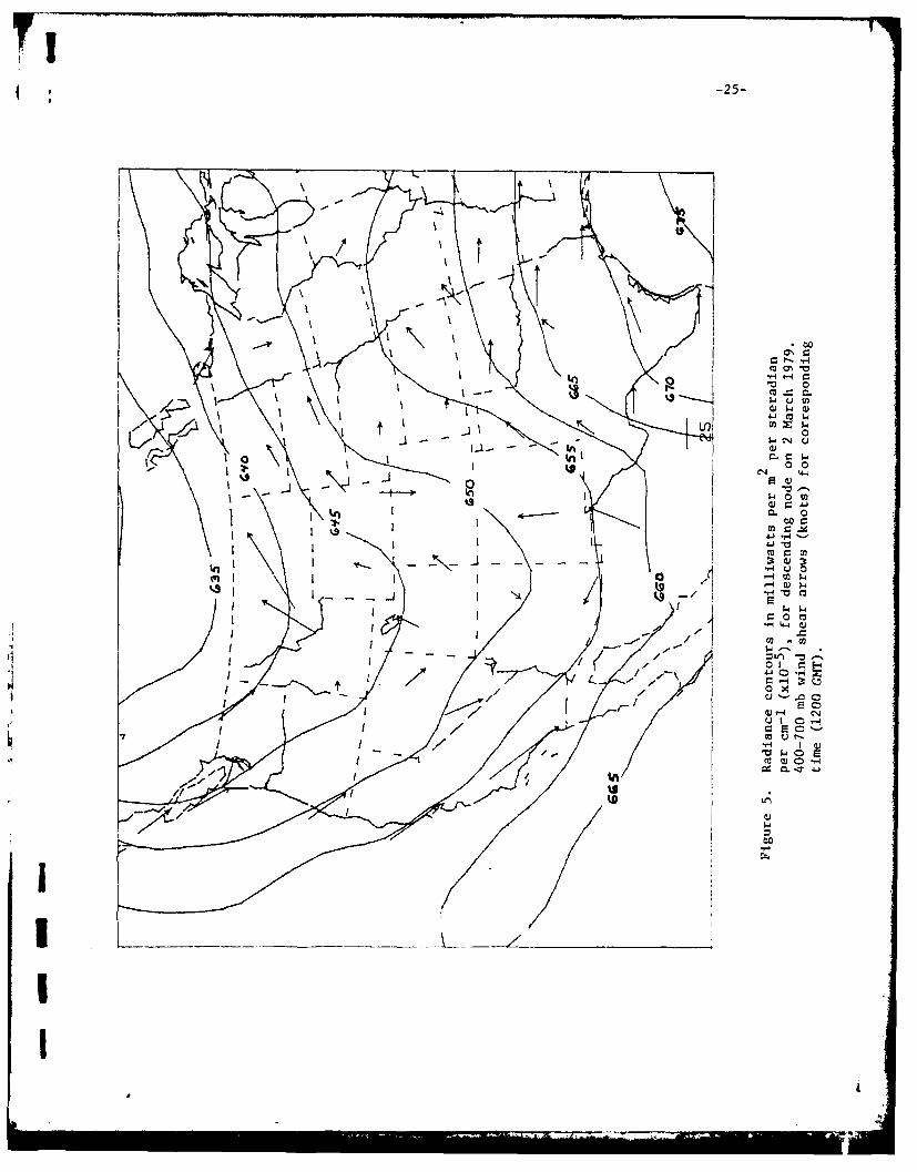
5 Radiance contours on 2 March 1979 with 400-700 mbwind shear arrows superimposed .... ............. ... 25

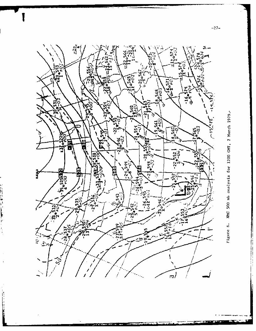
6 NMC 500 mb analysis for 1200 GMT, 2 March 1979 ....... 27

7 MSU channel 2 radiance analysis with 400-850 mb windshears at 1200 GMT 3 March 1979 superimposed ........ .. 53



10 HIRS channel 5 radiance analysis with 400-850 mb windshears at 1200 GMT 6 March 1979 superimposed ........ .. 56

11 MSU channel 2 radiance analysis for 7 March 1979. ... 57

12 MSU channel 2 radiance analysis with 400-850 mb wind 58

shears at 1200 GMT 7 March 1979 superimposed .........

13 HIRS channel 3 radiance analysis for 7 March 1979 .... 59

14 HIRS channel 4 radiance analysis for 7 March 1979 .... 60

j 15 HIRS channel 5 radiance analysis for 7 March 1979 . 61

16 HIRS channel 5 radiance analysis with 400-850 windshears at 1200 GMT 7 March 1979 superimposed ........ .. 62

17 HIRS channel 3 radiance analysis for 8 March 1979. . . . 63

I

I

-vii-

LIST OF FIGURES (continued)

Figure Page

18 HIRS channel 4 radiance analysis for 8 March 1979. . .. 64

19 HIRS channel 5 radiance analysis for 8 March 1979. . . . 65

4

I

-viii-

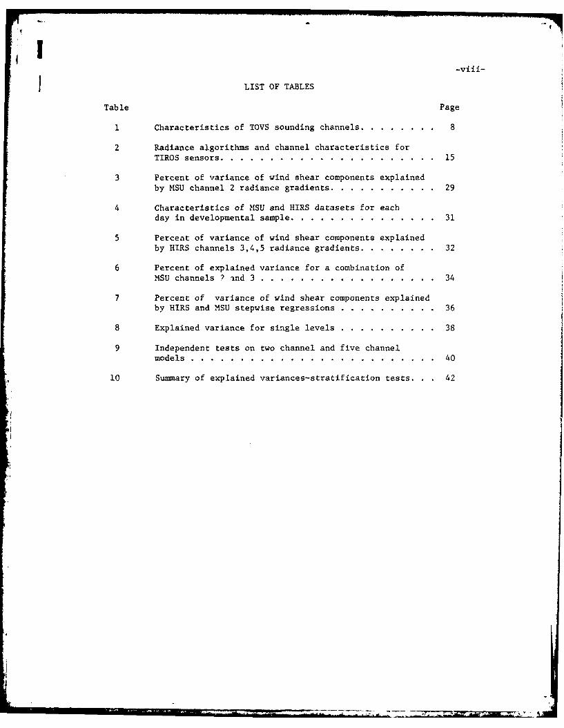
LIST OF TABLES

Table Page

1 Characteristics of TOVS sounding channels .... ........ 8

2 Radiance algorithms and channel characteristics forTIROS sensors ........ ...................... ... 15

3 Percent of variance of wind shear components explained

by MSU channel 2 radiance gradients ... ........... ... 29

4 Characteristics of MSU and HIRS datasets for eachday in developmental sample ..... ............... ... 31

5 Percent of variance of wind shear components explainedby HIRS channels 3,4,5 radiance gradients .... ........ 32

6 Percent of explained variance for a combination ofMSU channels ? and 3 ....... .................. . 34

7 Percent of variance of wind shear components explained

by HIRS and MSU stepwise regressions ... .......... . 36

8 Explained variance for single levels ... .......... . 38

9 Independent tests on two channel and five channel

models .......... ......................... ... 40

10 Summary of explained variances-stratification tests. . . 42

Estimation of Vertical Wind Shear from Infraredand Microwave Radiances

1. Introduction

The major purpose of the weather satellite program is to infer

meteorological data from space, especially in regions of sparse observations.

Estimation of winds presents special challenges, because satellites do not

presently carry sensors specifically designed for wind meas.r.--ent, although

satellite-borne lasers are under consideration.

So far, w%,i.-s have been obtained by use of three distinct methods:

backscatter from the sea surface, tracking of cloud elements and computations

from satellite-inferred temperatures.

Backscatter provides only surface winds, and is limited to oceanic

areas. Cloud motions require the presence of clouds (which cover only about

50% of the earth's surface), and clouds may not travel with the speed of the

wind. Further, cloud-tracing is only possible where distinct cloud elements,

such as those produced by convection, can be identified in successive images.

Lee (1979) showed that this technique is most useful in obtaining winds in

the low troposphere, near 800 mb.

The technique of inferring winds from temperatures can be used in the

j largest volume of the atmosphere, and is most commonly applied. This approach

can be considered to be operational, in the sense that the currently-

applied operational forecasting models include wind analyses that

are obtained from such calculations, at least over the oceans (Phillips

et al., 1979). Although there have been some recent encouraging

results reported by Phillips (1980), such wind estimates suffer from the

weaknesses implicit in the recovery of the temperature profiles, which must

I

-2-

be estimated first in order to calculate the hypothetical balance between

the wind field and the mass (temperature) field.

Recently Carle and Scoggins (1981) found that geostrophic winds

calculated from satellite-derived mass fields display secondary wind maxima

that are apparently spurious in the vicinity of the jet stream. Mean

differences between satellite-derived and radiosonde-derived geostrophic wind

-lspeeds were of the order of 5 m s and displayed standard deviations ranging

-1up to 12 m s near the jet stream in Carle and Scoggins'sample. They also

found that the satellite-based geostrophic winds systematically underestimated

the jet stream wind speed and its associated shear, consistent with the often

reported tendency for satellite-based temperature soundings to underestimate

the magnitude of the horizontal temperature gradient, where it is strong

(Carle and Scoggins, 1981).

Recently, Brodrick (1980) produced an encouraging case-study of jet-

stream winds on a cross section by calculating shear from temperatures

observed by TIROS-N. Smith and Togstad (private communication) have studied a

similar case to obtain a realistic jet stream mapping in a clear region. Also,

Smith et al. (private communication) have detected small-scale temperature

changes from a geostationary satellite, which might be useful in diagnosing

small-scale wind shear.

Wind information derived from radiances has some drawbacks: 1) The

vertical resolution is poor, 2) temperature information can be used directly

only to infer balanced wind shears, not winds at any one level, 3) the

transmission of infrared radiances is limited by clouds. Microwave radiances

penetrate clouds (not precipitation), but the vertical resolution of micro-

wave-derived winds is theoretically somewhat coarser than that obtainable from

infrared-derived winds. Perhaps optimum results can be achieved by combination

-3-

of infrared and microwave radiances. 4) The derived wind shears are related

to the mass field by theoretical relations which are subject to assumptions

which may not be completely satisfied.

In practice, it is desirable to infer winds rather than wind shears

from satellites. We can identify three distinct methods for obtaining winds,

given the possibility of estimating wind shears.

In the first case, it is assumed that winds are available at a particular

level from other information. For example, winds near 200 mb are quite well

known from jet aircraft and cirrus motions. Or, winds near 850 mb may be

available from motions of low-topped convective clouds. Combining these

winds with satellite-derived wind shears yields winds at other levels.

Alternatively, it is assumed that the sea level pressure field is known

from other information. Then, the satellite-derived temperatures yield the

pressure field and hence balanced winds. This technique is being used

successfully by NOAA at the University of Wisconsin, under the direction of

Dr. William Smith.

Finally, winds are obtained statistically from wind shears. It is known

empirically that wind shears between 1000 mb and 500 mb are quite well

correlated with the winds themselves at 500 mb, at least in middle latitudes.

Statistical relationships can be derived for these quantities. However,

coefficients may have to be stratified by region and season.

j In this project, we attempt to use the first and third of the methods

alove to infer winds from satellite radiance gradients. The use of horizontal

radiance gradients is advantageous in that the effects of systematic error in

the radiances are reduced.

I____. __ 2- ~-.4 • 4=", 2

2. Theory

Vertical wind shears were first derived from horizontal radiance

gradients by Zak and Panofsky (1968) who used the relatively crude measure-

ments on TIROS 7 to infer wind shears between 100 mb and 10 mb. They began

by putting (for a given narrow wavelength band)

R - W(z)I(T,z)dz0

where R is the radiance, W(z) a weight function which depends on height z

but is constant in the horizontal, and I is the contribution at each height

to the total radiance. T is temperature and I is a function of temperature

at height z.

Differentiating with respect to x, an arbitrary horizontal coordinate,

ax dl 3T

A similar equation holds in the horizontal y direction, at right angles to x.

If we assume geostrophic winds

3T fT 31 (2)3x g ;z

where v is the velocity component in the y-direction, f is the Coriolis

parameter and g is gravity. Then

yR fT Wz d 3va-x _9 TTg ToWz z d 3

I

!I

-5-

Similarly,

DR _ _ fT ddI _uaY g 0 dT WzW) -dz (4)

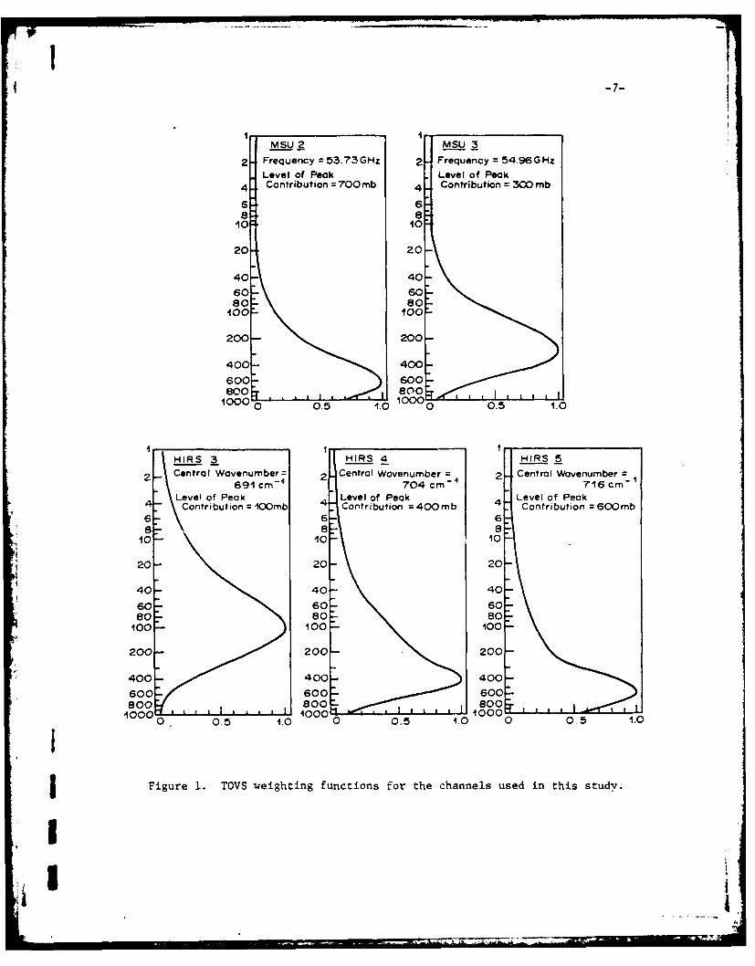
The functions W(z) and Lare well known. Figure l, taken from SmithdT

et al. (1979), shows W(z) for TIROS-N infrared and microwave channels used

in this report. The problem is to solve (3) and (4) for wind differences

between certain levels, given measured values of T and T in several channels

simultaneously.

This problem has been discussed by many investigators. Of special

interest here is the work by Fleming (1979) who showed that finite wind

differences between particular levels can be obtained from linear combinations

of radiance gradients in particular channels in the infrared region.

Such linear combinations can also be derived by regression analysis

which assures the statistically "best" representation of observed wind

differences or winds from a linear combination of radiance gradients. The

drawback of the statistical method is that the fit may provide coefficients

best suited only to the original (developmental) sample. Since they are not

based on physical reasoning, they may not be equally well suited to other

samples; hence it is essential that such equations be tested on independent

information.

Equations (3) and (4) are based on the geostrophic assumption, and

clearly lead to underestimates of wind shears in anticyclonic and over-

estimates in cyclonic regions. Because of this restriction, improved

statistical relationships could be derived by developing separate equations

in areas of contrasting curvature of the flow or by relating "errors" in the

equations to contour curvature.

-6-

3. Satellite data

The radiance data for this study were obtained from the Satellite Data

Services Division (SDSD) of the National Climatic Center (NMC). The TIROS-N

satellite, launched in October 1978, was the source for all satellite data.

To allow for several months of system shakedown time, the month of March 1979

was chosen for this pilot study.

The TIROS-N satellite is the first in a series of a new generation of

NOAA operational polar orbiting satellites. The orbital period is approximately

102 minutes resulting in 14.2 orbits per day. The satellite operates with

a southbound equator crossing time (descending node) at approximately 0300

Local Standard Time (LST) and a northbound equator crossing (ascending node)

at approximately 1500 LST.

The satellite is equipped with an instrument package known as the

TIROS-N Operational Vertical Sounder (TOVS) which consists of three instruments:

1) the second version of the High Resolution Infrared Radiation Sounder

(HIRS-2), 2) the Microwave Sounding Unit (MSU) and 3) the Stratospheric

Sounding Unit. Each instrument is a multi-channel radiometer which measures

the radiation emerging from the top of the atmosphere. For this study of

mid-tropospheric wind shear, only radiance data from HIRS-2 and MSU are used.

Table 1, adapted from Smith et al. (1979), gives a synopsis of the

characteristics of each of the various spectral channels used in this

research. Only channels 2 and 3 of the MSU and 3, 4 and 5 of the HIRS-2

were used here, because only these channels respond significantly to tempera-

tures in the middle troposphere (see Fig. 1).

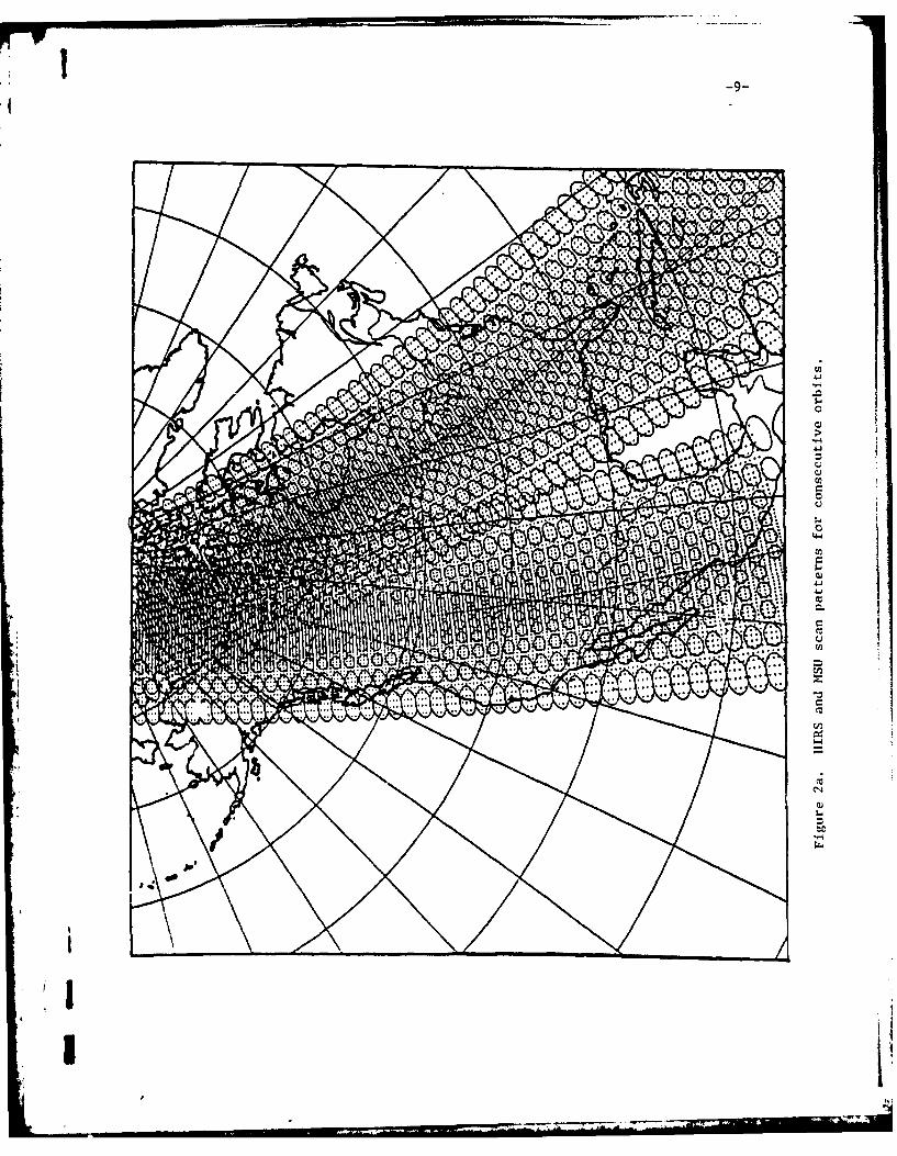
The scan pattern of the HIRS-2 and MSU instruments for two consecutive

orbits is shown in Fig. 2a. The HIRS-2 samples 56 fields of view (FOV) in a

!

!i

MSU 2 MSU 3

2 Frequency =53.73GHz 2- Frequency = 54.96GHz

Level of Peak Level of Peak4 Contribution =700mb 4- Contribution 3CO nb

6 68 8 a

10 40

20 20

40 40

60 6080 80

400'- 100-

200 200-

400- 400

600 600800' 8o00t

1000 0 0.5 1.0 0.5 1.0

HIRS 3 HIRS 4 HIRS 5

2 Central Wavenumber= 2 Central Wavenumber = 2 Central Wavenumber691 cm - 4 704 cm- 716 cm-

Level of Peak 4Levelof Peak Level of PeakContribution 100mb Contribution =400mb Contribution = 600mb

6 6 68 8 8

10 10 10

20 20 20-

40 40 40

60 60 6080 80 80

100 100 100

200 200- 200

400 400- 400

600 6001 600"800 800 800-O800 0 1000 01 0.5 1.o0 0 0.5 4.0 0 0.5 1.0

Figure 1. TOVS weighting functions for the channels used in this study.

F.au.!i

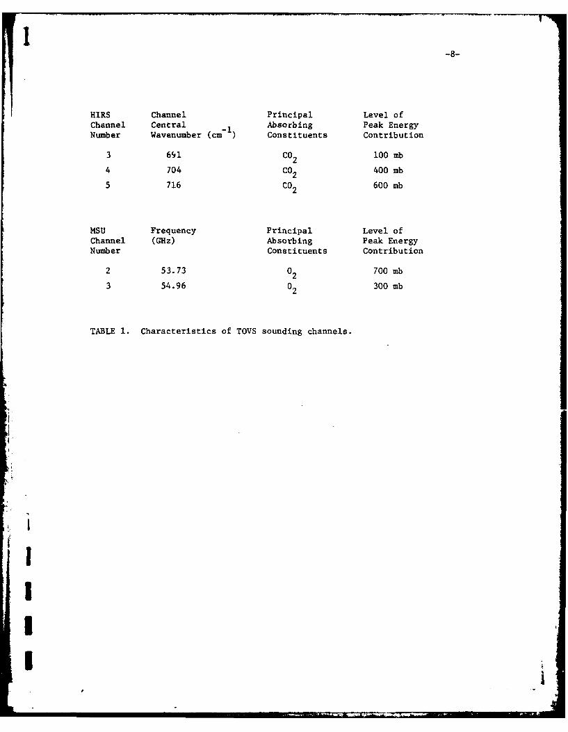
HIRS Channel Principal Level ofChannel Central 1 Absorbing Peak EnergyNumber Wavenumber (cm- ) Constituents Contribution

3 691 CO2 100 mb

4 704 C02 400 mb

5 716 CO2 600 mb

MSU Frequency Principal Level ofChannel (GHz) Absorbing Peak EnergyNumber Constituents Contribution

2 53.73 02 700 mb

3 54.96 02 300 mb

TABLE 1. Characteristics of TOVS sounding channels.

I

I

I

i

-9-

400

-10-

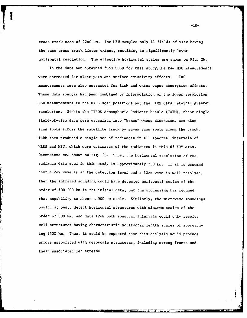
cross-track scan of 2240 km. The MSU samples only 11 fields of view having

the same cross track linear extent, resulting in significantly lower

horizontal resolution. The effective horizontal scales are shown on Fig. 2b.

In the data set obtained from SDSD for this study, the raw MSU measurements

were corrected for slant path and surface emissivity effects. HIRS

measurements were also corrected for limb and water vapor absorption effects.

These data sources had been combined by interpolation of the lower resolution

MSU measurements to the HIRS scan positions but the HIRS data retained greater

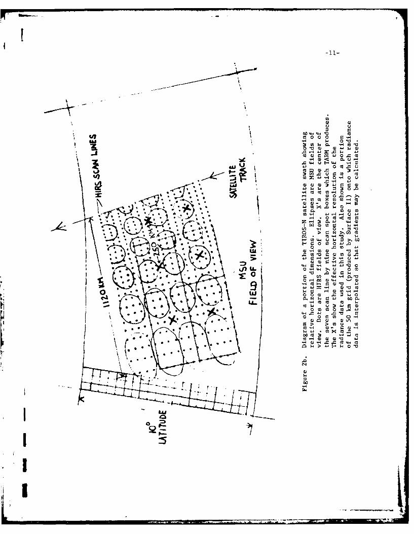
resolution. Within the TIROS Atmospheric Radiance Module (TARM), these single

field-of-view data were organized into "boxes" whose dimensions are nine

scan spots across the satellite track by seven scan spots along the track.

TARM then produced a single set of radiances in all spectral intervals of

HIRS and MSU, which were estimates of the radiances in this 63 FOV area.

Dimensions are shown on Fig. 2b. Thus, the horizontal resolution of the

radiance data used in this study is approximately 250 km. If it is assumed

that a 2Ax wave is at the detection level and a 1OAx wave is well resolved,

then the infrared sounding could have detected horizontal scales of the

order of 100-200 km in the initial data, but the processing has reduced

that capability to about a 500 km scale. Similarly, the microwave soundings

would, at best, detect horizontal structures with minimum scales of the

order of 500 km, and data from both spectral intervals could only resolve

well structures having characteristic horizontal length scales of approach-

ing 2500 km. Thus, it could be expected that this analysis would produce

errors associated with mesoscale structures, including strong fronts and

their associated jet streams.

06 c

-4 41- O' A

41 JI - 0 ~I0 =CIca~ 0 M)Q)x Dt

3r4 C4 Vu ca4.- H 00 -02 Cu

4JiI P $4 0 .0. 14- ca * Ii Cu 02~0

I ~ * 4 *0 Q)- Cu C

-H2 4 jr-4 0 0 to -c ar

.. t 1-4. 4 V 04 4

Cu4 To- "4 W

C-4 )~W M4.4U 0 tF-4 0 .0 m0 C41 .0

0 J-E4 Q)i 41

000

"-44

0 )I-4 0 acu1;

-12-

Because many cloud structures have smaller dimensions than the scales

discussed above, the smoothing of these data alleviates small-scale con-

tamination by clouds at the expense of resolution. However, elimination

of cloud-contaminated radiances also produces uneven spacing of the infra-

red radiance observations only. Infrared signals are subject to cloud

contamination which makes the satellite infrared fluxes appear colder than

they actually are. Within TARM, two methods are employed to correct for

cloud contamination. In one, called the clear search method, sufficient

holes are found in the clouds from whose uncontaminated measurements a

volume estimate can be obtained. If this method fails, the N* approach is

used,where physical and mathematical techniques are combined to obtain clear

column radiances from the contaminated ensemble. Additional details con-

cerning these methods are given by Smith et al. (1979); it is also discussed

in Appendix A.

In cloudy areas, infrared radiances are quite unreliable. In the first

sample, observations in these areas were deduced by interpolation. Later,

a second sample of HIRS-2 data was tested in which seriously cloud-contaminated

data were eliminated.

The TOVS sounding product tapes (Level 2A) used in this research contain

brightness temperature data. These brightness temperatures are weighted,

consisting of contributions through the depth of the atmosphere and are

characteristic of the measured radiation at the top of the atmosphere. In

order to test our hypothesis that horizontal radiance gradients relate

information about vertical wind shears, these brightness temperatures were

converted to radiances.

II

-13-

Information is extracted from the TOVS tapes in the form: DAY, TIME,

LATITUDE, LONGITUDE and TEMPERATURE. Because of the asymmetry in the FOVs

used for each box in the clear column radiance search, each latitude-

longitude coordinate point represents a weighted central position in the seven

scan line by nine scan spot box. In order to make the conversion to radiance,

a slightly different algorithm for the channels of both sensors is used.

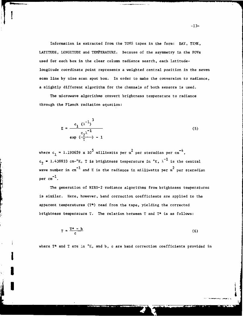
The microwave algorithms convert brightness temperature to radiance

through the Planck radiation equation:

E= c (5)

expc2l

5 m2 -4

where cI = 1.190659 x 10 milliwatts per m per steradian per cm

c = 1.438833 cm-*K, T is brightness temperature in OK, X- is the central-2

wave number in cm 1 and E is the radiance in milliwatts per m2 per steradian

-1per cm

The generation of HIRS-2 radiance algorithms from brightness temperatures

is similar. Here, however, band correction coefficients are applied to the

apparent temperatures (T*) read from the tape, yielding the corrected

brightness temperature T. The relation between T and T* is as follows:

T* c- b(6

where T* and T are in 'K, and b, c are band correction coefficients provided in

I~, I

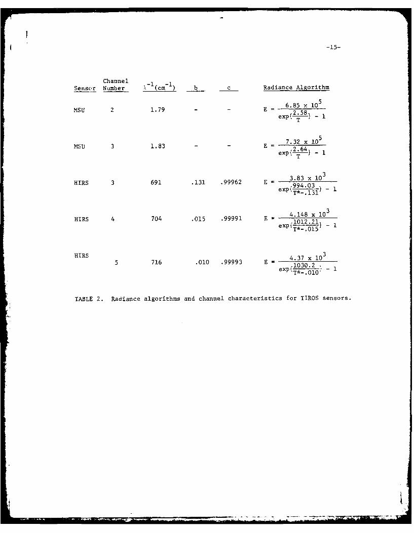
Table 2. The individual HIRS algorithms arc then computed as before using (5).

Table 2 lists the TIROS sensor algorithms used in this calculation.

Data sets on a latitude/longitude grid were created for each day and

channel in the form: TIME, LATITUDE, LONGITUDE and RADIANCE. In order to

test our hypothesis, a cartesian grid of horizontal radiance gradients was

constructed with the Y axis along the satellite track. This necessitated

a conversion of latitude-longitude coordinate radiances to a cartesian

system.

This conversion is accomplished by the specification of two parameters.

First the distance of the projected point from the pole is determined using

the latitude angle and trigonometry. Second, the angular difference between

the prime longitude and the longitude is computed, where the prime longitude

is defined as the meridian which is perpendicular to the base of the map

and which extends from the pole to the bottom of the map. These two

parameters lay the framework for the conversion of latitude-longitude

coordinate pairs to a cartesian grid on a polar-stereographic map with the

Y axis oriented along the satellite track.

By specifying the desired number of grid points between the pole and

the equator (100 was used here), a cartesian grid encompassing the North

American radiosonde network west of 850 west was established with each grid

point spaced about 100 km apart.

For use in this research, the geographic coordinates are the cartesian

coordinates x, y defined by the satellite track, with radiance at each

location constituting the independent variable (z). The only inherent

restrictions are that the coordinate variables must be orthogonal and the

z variable must be single valued.

r, I

4 -15-

Channel -I-Sensor Number \(cm ) b c Radiance Algorithm

Msu 1.7 E = 6.85 x 10 5

MSU 1.7 - -2.58

exp{ T-

Msu 1.8 - -E = 7.32 x 10 5

!4~U 31.83 E= 2.64,T

HIRS 3 691 .131 .99962 E = e.83 994.03

T*.131

HIRS 4 704 .015 .99991 E = 418x11012 21T*.015

HIS5 716 .010 .99993 E = -4.7x131030 2

expf{ OT*.010

TABLE 2. Radiance algorithms and channel characteristics for TIROS sensors.

-16-

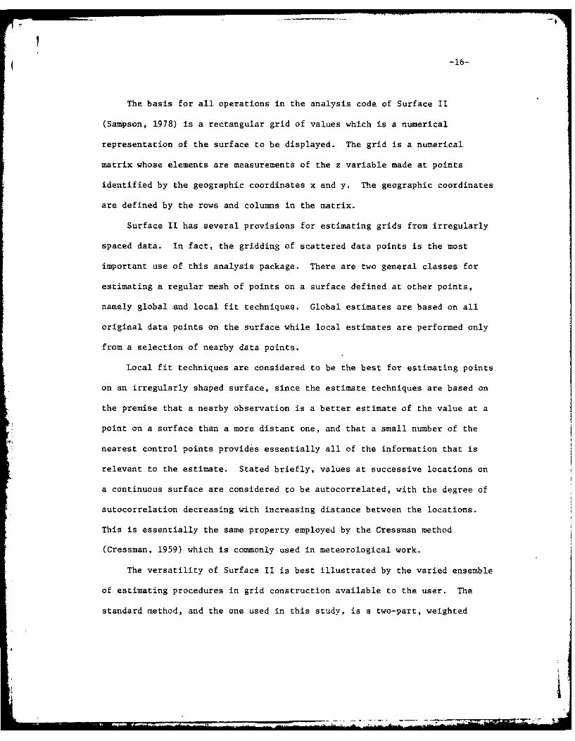
The basis for all operations in the analysis code of Surface II

(Sampson, 1978) is a rectangular grid of values which is a numerical

representation of the surface to be displayed. The grid is a numerical

matrix whose elements are measurements of the z variable made at points

identified by the geographic coordinates x and y. The geographic coordinates

are defined by the rows and columns in the matrix.

Surface II has several provisions for estimating grids from irregularly

spaced data. In fact, the gridding of scattered data points is the most

important use of this analysis package. There are two general classes for

estimating a regular mesh of points on a surface defined at other points,

namely global and local fit techniques. Global estimates are based on all

original data points on the surface while local estimates are performed only

from a selection of nearby data points.

Local fit techniques are considered to be the best for estimating points

on an irregularly shaped surface, since the estimate techniques are based on

the premise that a nearby observation is a better estimate of the value at a

point on a surface than a more distant one, and that a small number of the

nearest control points provides essentially all of the information that is

relevant to the estimate. Stated briefly, values at successive locations on

a continuous surface are considered to be autocorrelated, with the degree of

autocorrelation decreasing with increasing distance between the locations.

This is essentially the same property employed by the Cressman method

(Cressman, 1959) which is commonly used in meteorological work.

The versatility of Surface II is best illustrated by the varied ensemble

of estimating procedures in grid construction available to the user. The

standard method, and the one used in this study, is a two-part, weighted

-17-

average of the projected slopes from the nearest neighboring data points

about each grid point. During the first pass, the slope of the surface is

estimated at each data point. The search procedure finds the n nearest

neighbors to the data point being considered and fits a weighted trend surface

to the point. Weights inversely proportional to the distance from the data

point being evaluated are assigned to the other points. Next, a constant of

the fitted regression equation is adjusted in order to guarantee that the plane

passes through the data point. If the search procedure does not find at

least 5 points or if the simultaneous equations of the fitted plane have no

solution, then the coefficients of a global trend are used as the local trend.

The second part of the method estimates the value of the surface at the

grid nodes. A search technique locates n' nearest neighbor data points about

each grid node. The x, y coordinates of the grid node are then substituted

into each of the local trend-surface equations associated with these points.

The result is a projection of these local surfaces to the grid node location.

A weighted average of these estimates is then calculated with each slope

weighted by the inverse of the distance between the grid node and the data

point associated with the slope.

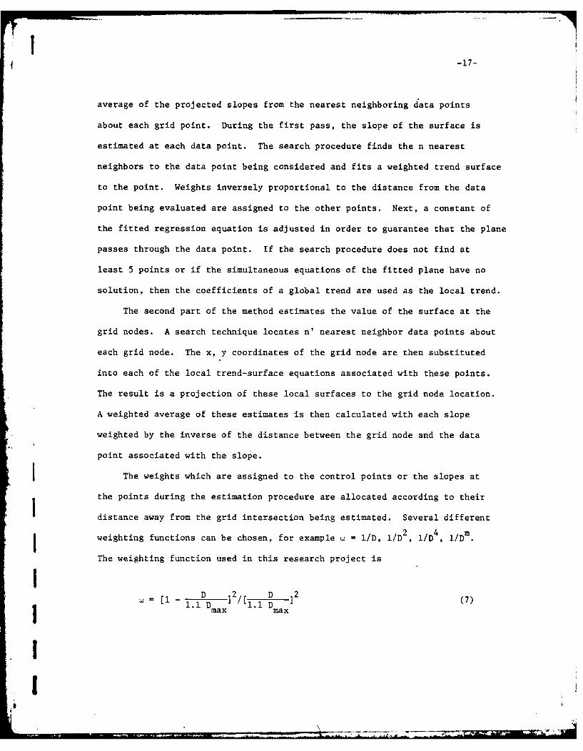
The weights which are assigned to the control points or the slopes at

the points during the estimation procedure are allocated according to their

distance away from the grid intersection being estimated. Several different

2 4mweighting functions can be chosen, for example w = l/D, l/D2 , l/D, /Dm .

The weighting function used in this research project is

ID 2 D ]2(7

1.1 D 2/1.1 D(7i~i ma x max

II

-18-

where w is the weight attached to a sample data point a distance D from the

grid intersection being estimated. D represents the distance from the gridmax

intersection to the most distant sample point in the set being used in the

estimation.

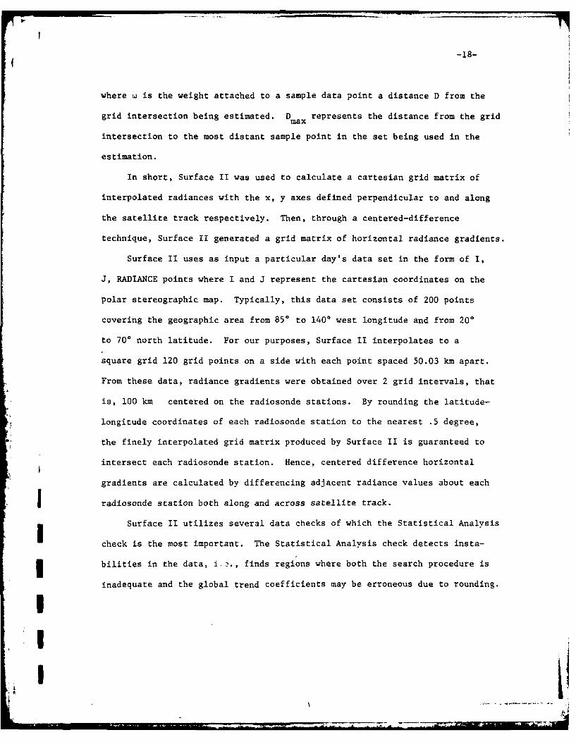
In short, Surface II was used to calculate a cartesian grid matrix of

interpolated radiances with the x, y axes defined perpendicular to and along

the satellite track respectively. Then, through a centered-difference

technique, Surface II generated a grid matrix of horizontal radiance gradients.

Surface II uses as input a particular day's data set in the form of I,

J, RADIANCE points where I and J represent the cartesian coordinates on the

polar stereographic map. Typically, this data set consists of 200 points

covering the geographic area from 850 to 140' west longitude and from 200

to 700 north latitude. For our purposes, Surface II interpolates to a

square grid 120 grid points on a side with each point spaced 50.03 km apart.

From these data, radiance gradients were obtained over 2 grid intervals, that

is, 100 km centered on the radiosonde stations. By rounding the latitude-

longitude coordinates of each radiosonde station to the nearest .5 degree,

the finely interpolated grid matrix produced by Surface II is guaranteed to

intersect each radiosonde station. Hence, centered difference horizontal

gradients are calculated by differencing adjacent radiance values about each

radiosonde station both along and across satellite track.

Surface II utilizes several data checks of which the Statistical Analysis

check is the most important. The Statistical Analysis check detects insta-

3 bilities in the data, i ., finds regions where both the search procedure is

inadequate and the global trend coefficients may be erroneous due to rounding.I'I I

-19-

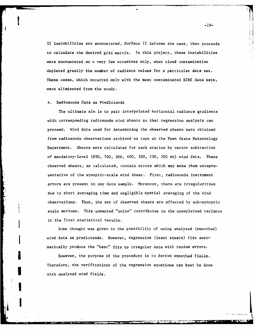
If instabilities are encountered, Surface II informs the user, then proceeds

to calculate the desired grid matrix, In this project, these instabilities

were encountered on a very few occasions only, when cloud contamination

depleted greatly the number of radiance values for a particular data set.

These cases, which occurred only with the most contaminated HIRS data sets,

were eliminated from the study.

4. Radiosonde Data as Predictands

The ultimate aim is to pair interpolated horizontal radiance gradients

with corresponding radiosonde wind shears so that regression analysis can

proceed. Wind data used for determining the observed shears were obtained

from radiosonde observations archived on tape at the Penn State Meteorology

Department. Shears were calculated for each station by vector subtraction

of mandatory-level (850, 700, 500, 400, 300, 250, 200 mb) wind data. These

observed shears, as calculated, contain errors which may make them unrepre-

sentative of the synoptic-scale wind shear. First, radiosonde instrument

errors are present in any data sample. Moreover, there are irregularities

due to short averaging time and negligible spatial averaging of the wind

observations. Thus, the set of observed shears are affected by sub-synoptic

scale motions. This unwanted "noise" contributes to the unexplained variance

in the final statistical results.

Some thought was given to the possibility of using analyzed (smoothed)

j wind data as predictands. However, regression (least square) fits auto-

matically produce the "best" fits to irregular data with random errors.

However, the purpose of the procedure is to derive smoothed fields.

Therefore, the verifications of the regression equations can best be done

with analyzed wind fields.

!7r,

-20-

A prime consideration in the analysis of data for this study was the

need to have the observed radiosonde data correspond as closely as possible

in time with the satellite radiance data. Given the satellite equator

crossing times of 0300 LST and 1500 LST and the radiosonde observation times

of 0000 GMT and 1200 GMT, it was decided that the western United States and

Canada would be chosen as the target region for this study. In this part

of the world, 0000 GMT corresponds to 1500-1700 LST and 1200 GMT corresponds

to 0300-0500 LST. As a result of satellite malfunctions, nearly all of the

radiance data near the 0000 GMT radiosonde observation time were missing

from the March 1979 data archive. This reduced the size of the data sample

by approximately half; however, sufficient 1200 GMT satellite data were

available to permit a pilot study.

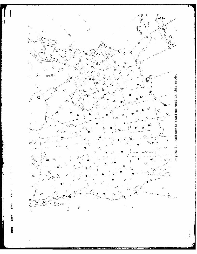
There is a relatively high density of radiosonde stations in the

United States portion of the area, but rather few in Canada. In the final

calculations, up to 46 radiosonde stations west of .85 W and east of 140 W

between 25 N and 70 N were used (Fig. 3). In that area, the time difference

between satellite and radiosonde observations ranged from nearly exact

correspondence at the western edge to about three hours difference at the

eastern edge. Allowing for the usual early release of tne radiosonde by

about one hour, the time correspondence may have been slightly better.

5. Statistical Technique

All of the correlations and regressions presented in this paper were

calculated through the use of the Statistical Analysis System, a commercially

,1I

0..yx0

0 0

00

..

00-

' ~4 e

d-c: 0 \V

.0 '

*r 0-! 0.1 0

0.0

01 \ -0 ~ ~oil 0 ~ 0*

0 : 0

~ J\ 0.

.0

00

C!C0 (0 *o 0. * G

0,0

0'0

0--

4 . z 0

-22-

produced statistical package avail-!1, at many IBM computer installations.

The procedure chosen to develop the linear regression equations was

forward stepwise selection. In this method, the first predictor chosen is

the one which has the highest correlation with the predictand. In each

subsequent step of the selection process, the predictor chosen is the one

which, when added to the equation, leads to the greatest reduction in

variance.

Of major concern in the linear regression approach, is the determination

of the optimum length of the equation. Including too many predictors in a

regression equation can result in the overfitting of tie equation to the

developmental sample. As a rule, the smaller the developmental sample, the

fewer should be the predictors allowed to enter the regression equation

(Lorenz, 1977).

Statistical significance tests are often used to determine the cutoff

point for the addition of predictors. However, such tests are not strictly

applicable here because meteorological observations are not independent of

one another. Weather typically occurs in regimes several thousand kilometers

in length. Thus, the horizontal scale of systems far exceeds the distance

jbetween radiosonde observations. As a result, two separate radiosonde

observations are not usually statistically independent.

The best avaiiable test for the reliability of an equation derived in

these circumstances is an independent test of another set of data. In this

pilot study, data from the first twenty-one days of March 1979 were used as

the developmental sample. ITie last ten days of the month were set aside as

the independent sample.II

_!

-23-

6. Experiments and Results

a. Characteristics of single channels

The early stages of data analysis for this study consisted of the pre-

paration of many radiance maps for a single channel. Appendix B shows

several examples of these radiance maps for each of the channels used in

this study. This map preparation was done to gain insight into the relation-

ship between the radiance and wind shear fields which would later be explored

statistically. In this pilot study, it was decided that the microwave

channels would be explored first since they are seldom contaminated

and yield the larger data base for use in statistical analysis. MSU channel

2, whose weighting function peaks near 500 mb, was judged as being the most

potentially useful single channel.

Figure 4 is a map of MSU channel 2 radiance contours together with

arrows which show the calculated values of mid-tropospheric (700-400 mb)

wind differences at 1200 GMT on 8 March 1979. The magnitude of the shear

is proportional to the length of the wind arrow (see scale Fig. 4). The case

is quite typical of many of the MSU channel 2 mappings. It can be seen

that there is a generally good correspondence between satellite-derived

contour orientation and observed 700-400 mb shears. In addition, information

about the position of the mid-tropospheric jet appears to be present; tight

radiance contour spacing from western Washington and Oregon into Wyoming

is associated with large shear magnitudes in this region. The small shears

in Montana and along the southern United States border are also linked with

smaller radiance gradients in this region.

Figure 5 is a similar map based on data for 1200Z on 2 March 1979.

This case is presented to highlight severe inconsistencies which appear

occasionally between observed and satellite derived shears. Note that while

I

-24-

14 00

0 0

/4 0W r. 4

4 O Xj

t.9 r-4 W $4

Q) wro

~~~~~~~~~~~1~~~$ $4-- - - - - - - ~ . - - _ _ _

rIN_ __A

-25-

\n "/ -4 C

I In

1 I4

I0 w

-4 0

=u0 1W~$~0

C-- -

0) 14ej 16 ,

cc Q. fl

!-26-

the overall patterns still correspond quite well, the observed shears at

Winslow and Tucson, Arizona and at Denver, Colorado are nearly opposite of

what would be expected from radiance contours.

The RIC analyses of the upper air conditions as well as the soundings

from Tucson and Winslow were examined closely for this case. A portion of

the analysis for 500 mb is shown in Fig. 6. A sharp trough axis through

central Arizona is apparent. At lower levels a small pocket of cold air

existed in southern Arizona and northern Mexico. It is probable that the

scale of this sharp feature cannot be resolved with these coarse microwave

data. Moreover, the strong cyclonic curvature of the streamlines at low

levels appears to be decreasing with height, introducing a difference

between the radiance gradient and the observed shear. The actual wind dif-

ference exceeds the thermal wind difference in flow becoming more anti-

cyclonic upward and vice-versa; in any region of strong vertical

change of curvature of the streamlines, systematic errors should appear.

If this is a case where sub-grid scale phenomena affect the observed

shears, verification on smoothed rather than actual wind shear as the

predictand should improve the agreement.

To give some quantitative idea of what can be obtained from a single

microwave channel, a regression experiment was performed with MSU channel 2

only. The data set used was a subset of the 1-21 March 1979 developmental

data sample consisting of 550 points on 19 days. In an effort to minimize

the effect of the interpolation technique on the final results only those

days with the greatest number of data points were used. Fractions of

explained variance values were then calculated for many combinaticns of shear

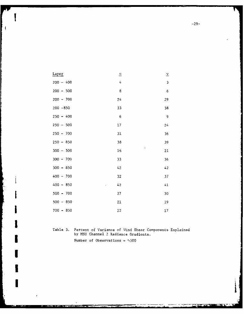
layers. Table 3 shows these values for the layers tested. Regression analy-

sis (least squares) is used to fit smooth curves to "noisy" data. The "noise"

- Ii- --. m.- Y. 1a

-27-

N - J*~;

J"V.

td,-

On 0)

-I \&1 ON,

I-

- -. *

4-Lntr

Nt

I,,M

!-28-

then becomes part of the 6,Lexplained variance. There is no point to smooth

the predictands first, because this smoothing is subjective, and reduces the

degrees of freedom. For these reasons, we chose directly observed vertical

differences of radiosonde wind components u and v as predictands, as well as

u and v components at particular levels. Wind speed and direction are less

satisfactory, because the significance of directions depends on speed; u

and v have better statistical properties. Best results are obtained for shears

between 850 mb and 300 mb, although 850-400 mb is nearly as good. It is seen,

however, that 850-500 mb shears are not accounted for nearly as well by

radiance gradients in this channel. The reason is clear: the weight function

for MSU channel 2 peaks at 500 mb, so that the weights of the winds at the

two levels peak above and below 500 mb, respectively.

There is a tendency (possibly not significant) for the fraction of v

components explained to be slightly larger than that of the u-components.

But in this sample, the v-components have slightly larger total variances, so

that their prediction error (see later section) tends to be larger.

Theoretically, HIRS channels should yield better results than MSU channels

since the weighting functions associated with infrared channels have more

sharply defined peaks. Hence, the HIRS channels were first tested indepen-

dently of the MSU channels to explore this contention.

The loss of data in the sample, which was related to instrument failure

jand contamination of infrared signals by cloudiness, presented challenges in

the analysis of the HIRS data. Unfortunately, certain aspects of the HIRS

results presented here seem to be a result of these sampling problems.

Once again, a subset of the 21-day developmental sample was chosen such

that only the most data rich days were included. Because of retrieval

problems, in fact, observations from only 9 days were used with only 275

-29-

Layer u v

200 - 400 4 3

200 - 500 8 6

200 - 700 24 29

200 -850 33 38

250 - 400 6 9

250 - 500 17 24

250 - 700 31 36

250 - 850 38 39

300 - 500 16 21

300 - 700 33 36

300 - 850 42 42

400 - 700 32 37

400 - 850 42 41

500 - 700 27 30

500 - 850 21 19

700 - 850 22 17

ITable 3. Percent of Variance of Wind Shear Components Explained

by MSU Channel 2 Radiance Gradients.

Number of Observations = 1500

II

I

-30-

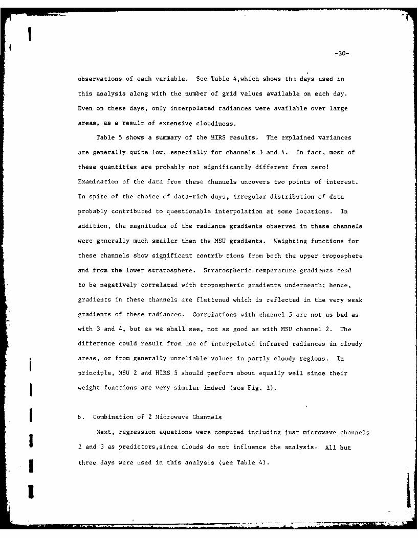
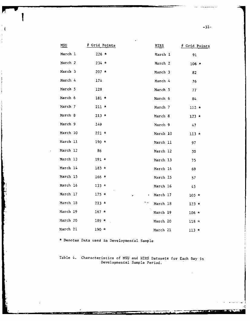
observations of each variable. See Table 4,which shows th, days used in

this analysis along with the number of grid values available on each day.

Even on these days, only interpolated radiances were available over large

areas, as a result of extensive cloudiness.

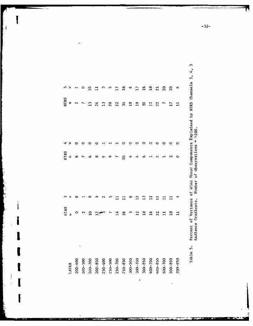
Table 5 shows a summary of the HIRS results. The explained variances

are generally quite low, especially for channels 3 and 4. In fact, most of

these quantities are probably not significantly different from zero!

Examination of the data from these channels uncovers two points of interest.

In spite of the choice of data-rich days, irregular distribution of data

probably contributed to questionable interpolation at some locations. In

addition, the magnitudes of the radiance gradients observed in these channels

were generally much smaller than the MSU gradients. Weighting functions for

these channels show significant contrib, tions from both the upper troposphere

and from the lower stratosphere. Stratospheric temperature gradients tend

to be negatively correlated with tropospheric gradients underneath; hence,

gradients in these channels are flattened which is reflected in the very weak

gradients of these radiances. Correlations with channel 5 are not as bad as

with 3 and 4, but as we shall see, not as good as with MSU channel 2. The

difference could result from use of interpolated infrared radiances in cloudy

areas, or from generally unreliable values in partly cloudy regions. In

principle, MSU 2 and HIRS 5 should perform about equally well since their

weight functions are very similar indeed (see Fig. 1).

b. Combination of 2 Microwave Channels

Next, regression equations were computed including just microwave channels

2 and 3 as predictors,since clouds do not influence the analysis. All but

three days were used in this analysis (see Table 4).

1!

-31-

MSU # Grid Points HIRS # Grid Points

March 1 226 * March 1 91

March 2 234 * March 2 106 *


March 4 174 March 4 76



March 7 211 * March 7 112 *

March 8 213 * March 8 123*


March 10 221 * March 10 113 *

March 11 190 * March 11 97


March 13 191 * March 13 75

March 14 183 * March 14 69

March 15 166 * March 15 57

March 16 133 * March 16 45

March 17 175 * , March 17 105 *

March 18 213 * March 18 123 *

March 19 167 * March 19 106 *

March 20 189 * March 20 118

March 21 190 * March 21 113 *

• Denotes Data used in Developmental Sample

Table 4. Characteristics of MSU and HIRS Datasets for Each Day inDevelopmental Sample Period.

-32-

In > _40 -4 cn U- r4 Q r- z '0 -4 0 0 '0 Q-4 -1 14 - 4 1- C N c'Jq

-4~ CJ o4~ r- c,) -i 0 c,4 t~ o 0' 0 c,4 " r-. r- -4 cfl,-4 Oq -1 J CN4 M '-4 M -i C4I -4 -4 o

I-q 0

=-4

CO-4)0

0.

u ca

-4> 000 C )Cj#nr -r4 M 0 4 -4 00 0 0 00 -4

~ Or. 0 o a r. .4 -4 1-4 1-4 1 -4 CN 0 c-44

~0

C'~> 0 '- CC a' CD 0P 0- 0- CD CDJ 0 0' r-- c- -D C

c- 0n 0 a r-. t '0 L M~ CD .4 a' -4 LM--47LM f 0 I L.4 r- G ,4 r-c r- co r- 00 -4m

U-1 Ln Ln L

clq li N ci cl -I cn (1) T L 0

-33-

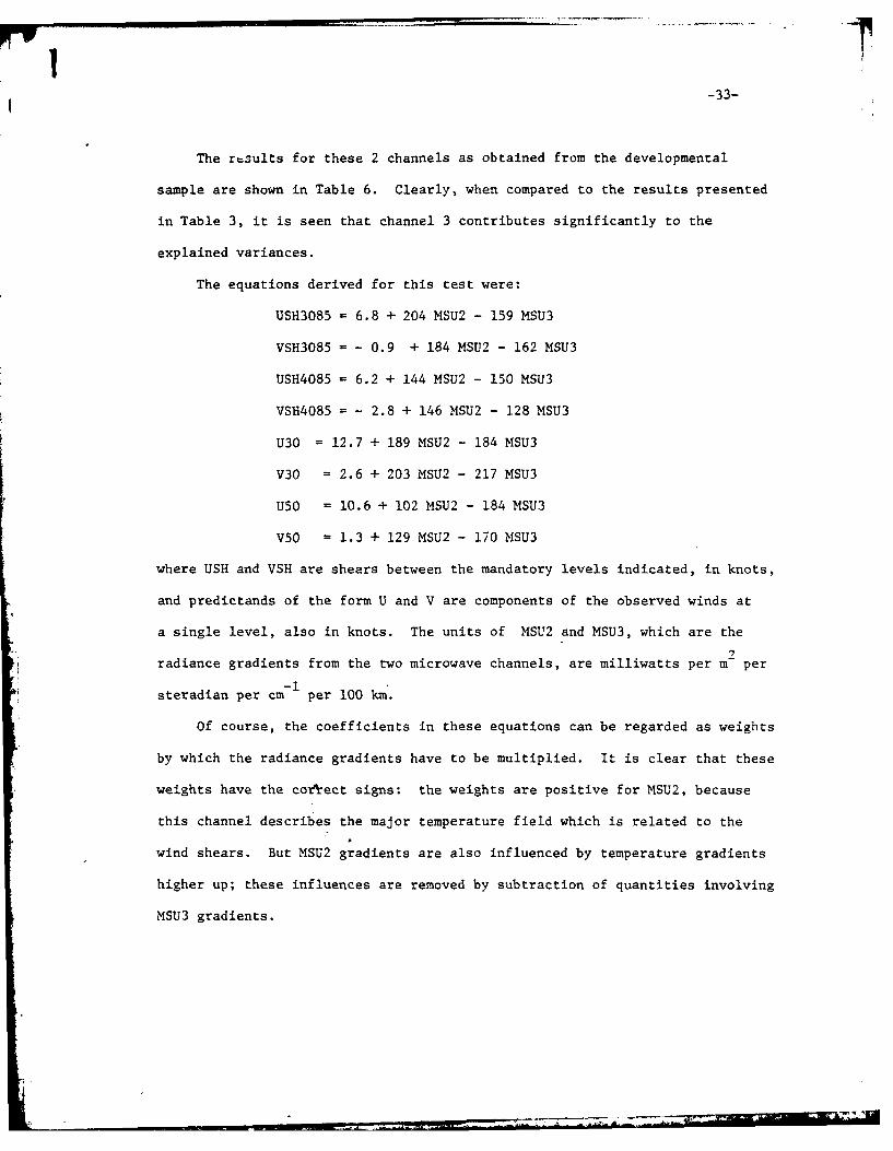
The results for these 2 channels as obtained from the developmental

sample are shown in Table 6. Clearly, when compared to the results presented

in Table 3, it is seen that channel 3 contributes significantly to the

explained variances.

The equations derived for this test were:

USH3085 = 6.8 + 204 MSU2 - 159 MSU3

VSH3085 = - 0.9 + 184 MSU2 - 162 MSU3

USH4085 = 6.2 + 144 MSU2 - 150 MSU3

VSH4085 = - 2.8 + 146 MSU2 - 128 MSU3

U30 = 12.7 + 189 MSU2 - 184 MSU3

V30 2.6 + 203 MSU2 - 217 MSU3

USO = 10.6 + 102 MSU2 - 184 MSU3

V50 = 1.3 + 129 MSU2 - 170 MSU3

where USH and VSH are shears between the mandatory levels indicated, in knots,

and predictands of the form U and V are components of the observed winds at

a single level, also in knots. The units of MSU2 and MSU3, which are the2

radiance gradients from the two microwave channels, are milliwatts per m per

steradian per cm- 1 per 100 km.

Of course, the coefficients in these equations can be regarded as weights

by which the radiance gradients have to be multiplied. It is clear that these

weights have the correct signs: the weights are positive for MSU2, because

this channel describes the major temperature field which is related to the

wind shears. But MSU2 gradients are also influenced by temperature gradients

higher up; these influences are removed by subtraction of quantities involving

MSU3 gradients.

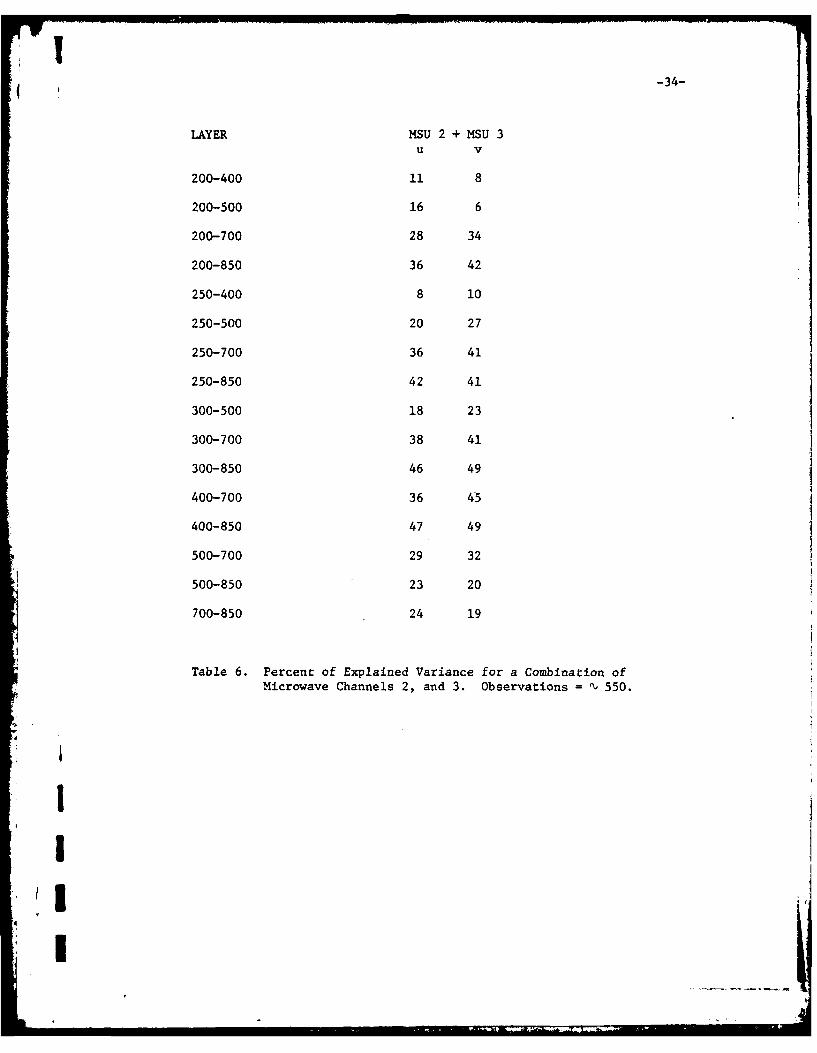
-34-

LAYER MSU 2 + MSU 3u v

200-400 11 8

200-500 16 6

200-700 28 34

200-850 36 42

250-400 8 10

250-500 20 27

250-700 36 41

250-850 42 41

300-500 18 23

300-700 38 41

300-850 46 49

400-700 36 45

400-850 47 49

500-700 29 32

500-850 23 20

700-850 24 19

Table 6. Percent of Explained Variance for a Combination ofMicrowave Channels 2, and 3. Observations = % 550.

II

I

-35-

c. Combinations of Microwave and Infrared Channels

Experiments were next performed in which two MSU and three HIRS channels

were combined in a stepwise regression procedure in which observed wind

shears were the predictands. Because HIRS coverage was poor on some days,

only 9 days were used.

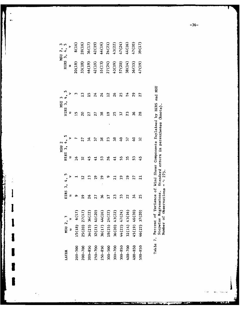
Table 7 summarizes explained variances and standard errors of estimates

(in parentheses) for these experiments. All possible shears between mandatory

levels in the 850-200 mb domain were tested, but only the layers displaying the

best correlations are included in Table 7 along with other layers of interest.

The highest correlations result for wind shears involving 850 mb, with the

other level being in the upper troposphere. Infrared channels alone are

disappointing; adding MSU 2 to them is helpful. The further addition of the

infrared channels, increases the explained variances, but the standard errors

do nlt decrease significantly by inclusion of the infrared channels. The

smallest standard errors result for the 700-460 w.b shears and the 850-250 mb

shears, because of their smaller variability in our sample. Standard errors

are likely to vary more among samples than correlations.

The rather poor performance of the infrared channels, particularly HIRS 2,

could be due to use of interpolated values in cloudy regions. To test this

possibility, another sample was collected from all 21 developmental days, but

restricting the analyses only to areas were the HIRS coverage was good. The

statistics did not improve substantially. This result indicates that the

poor performance of HIRS channels must be due to the unsatisfactory retrieval

techniques even in only partly cloudy areas. Overall, the results are not

likely to be superior to alternative methods that generate root-mean-square

n e-1Iwind errors of order 5 ms .Also, as with MSU2 alone, the results involving

II

-36-

cnLM ,o %.o r- O 0% 0 r-i (-4 T7 . 0 P~ -- -4 .- 4 -4 C14 N- - -1 C-I -4

C-4- M T- --T ~ -4r I- 0

w m % 0% CY'l m~ IT % 0 -T U, cy%4- 4-4 -4 -4 -I C 4 - -I -

0 Ln r- , C- M~ r. W '0 fl-M- 'T -r LM "- -T V)~ M ul -IT

~En

> m -M n-It 'T C- 1 4 %0 I C - T C-I r-

-4~~~- Clr-)"C4

,

04

Cd) 0

> -I0 C-4 m, C -4 0 0 -4N U, UZ rU1 -4 -4 -4 U, 1-I -7 U -1 U, 00

*0

U, %D r n e C4 - / ) c~ H-

-~ 4 C4 M 4 M C4 M( N (N 4

-7:

.- C-I C-''4 . 4 ( T zN 0' C-

>~)CO

00 , CU 0 , 0 , UU,4 C-4. Cn M- 4 M, C- Cn C - T

0 - nV) C n LI o -o m r- 0 1 0 0..................

-37-

the 500 mb level are notably inferior to those involving 400 mb and higher

levels.

It is noteworthy that the explained variance of the east-west component

is larger than that of the north-south component in the cases where infrared

predictors are used. This reverses a slight v-component superiority for the

MSU2 predictor test reported in Table 3. That was explained in terms of

somewhat greater u-component variability in the sample. A direct comparison

cannot be made here, however, because the sample size has changed. However,

it is worth noting that the standard deviations of u-components in this

smaller sample average 4 to 6 knots less than the standard deviations of the

v-componehts. It is believed that these differences are an artifact of the

sample, and not of the atmosphere.

It. middle latitudes, there tends to be a strong correlation between

the wind shear and the wind itself at the higher altitude levels. For

example, the 500-1000 mb shear is usually dominated by the 500 mb wind. In

the preceding analyses, the 850-300 mb shear has exhibited relatively high

j correlations with radiance gradients. This suggests the possibility of

estimating winds directly at a level in the upper troposphere from radiance

gradients.

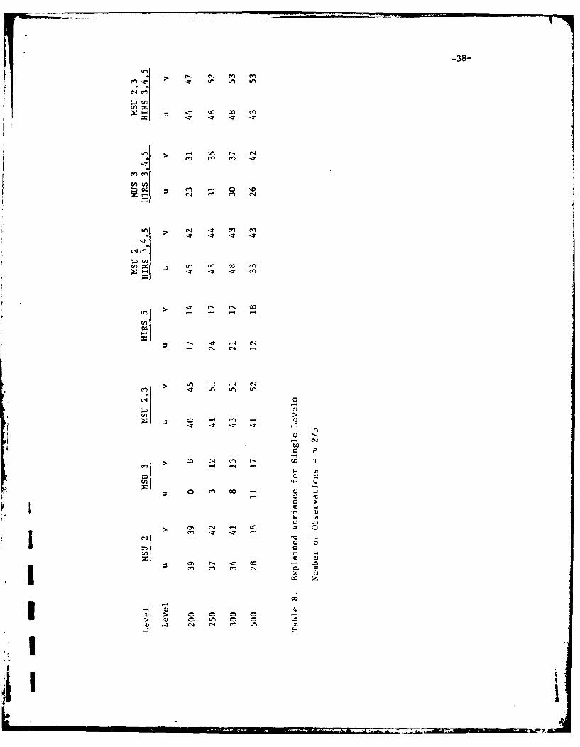
Thus, experiments were performed correlating the observed winds with

radiance gradients for several mandatory levels. Results are summarized in

Table 8. The general pattern of previous results remains the same; MSU

channels 2 and 3 contribute the bulk of the information. The 300 mb winds are

I correlated with the radiance gradients of these channels. Indeed, the results

are almost as good as those obtained for the 850-300 mb layer. Theoretically,

I wind shears should be predicted more accurately than single level winds.

However, shears are noisier than the winds themselves and this may cancel the

I

-38-

2~00 0

-4U4 r

en en ,-n C

C14 cn M C'4

Ln > C 4 -Z o

In!

:T r- - 0

.- 4 - -4

44 r-4

r-44

-4~- cn IJ a

00

co. C14 -n 00

U ~J 0-4 4-

0~ en 00 00-4 .

-4

- > CS 0 04 0 0-

r, 00 0 0 .

w > N a' C4> )Iii 4cnL

-39-

theoretical advantage. Thus, these results suggest the possibility of

obtaining winds at a level statistically from radiance gradients. Coefficients,

however, may have to be stratified by region and season.

d. Independent Tests

Because of the small sample size, it is essential to test the equations

on independent data. This was done from data taken during the last 11 days

of March, for which nine provided satisfactory data in the HIRS channels.

The equations were tested by two methods: in the first, raw shears were

computed by vector differences of mandatory-level winds just as they had been

in the developmental sample. The Cartesian components were then correlated

with values predicted by the above equations.

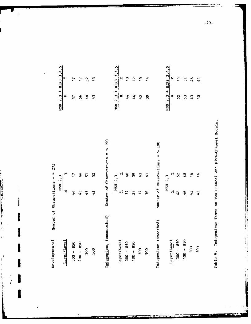
Since the equations led to smoothed fields, they were also tested on

horizontally smoothed observations. This smoothing was accomplished by a

Cressman analysis scheme on a 30 x 40 grid (grid spacing approximately 90

km) which was overlaid on a polar sterographic map of the target area.

Also a pass was made with a 1-4-1 smoother. Table 9 shows the results.

There is a considerable loss of explained variance as one goes from the

developmental sample to the unsmoothed independent sample. This, of course,

is typical of independent testing of regression equations. Interestingly,

however, results improve by a large amount when the equations are tested on

the smoothed sample. This is not surprising since regression should handle

the noise in the developmental sample in an optimum fashion. However, this

improvement is less for the winds than the wind shears, since winds have less

random error. Caution must be used in generalizing from this independent

test due to the small size of the developmental and independent samples.

Nevertheless, the last section in Table 9 is likely to give the best

idea how well regression is likely to predict winds and wind shears from MSU

I

-40-

->1 ~ c.W Ir I n n -T -.T -T - n T I

cn r- \0 00 cn w -Z '3. CN C7% m :2 CN en en~* £j U) IT IT - 7 IT m ~ C-n Wr u)

*0

W >0' 0 ;

Ln 0rii

ITl -dL ) c T n I . n Ln -3 r '

Lt 4 0o C 100

0 fn,

:r N n C- -4 r- co r , 0 v~ CC~ -4 CN Ln

.0(j2 00

.00

k '4 '14

0 .0c . V 0 00 0

I CD2 a Wu" l L

01 CD C ~ 00

> ~i

4-.

-41-

data only, in middle latitudes. Further improvement should be possible by

correcting for the deviation of actual from geostrophic winds.

Without such correction, then, we expect to account for about 50% of

the variances of middle-troposphere layers, and somewhat less for the winds

themselves, by the statistical techniques (correlations of order 0.7).

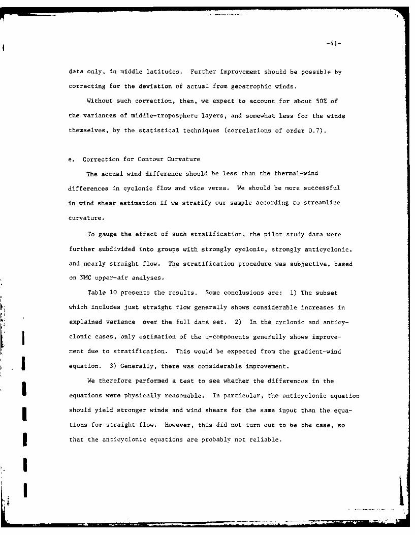
e. Correction for Contour Curvature

The actual wind difference should be less than the thermal-wind

differences in cyclonic flow and vice versa. We should be more successful

in wind shear estimation if we stratify our sample according to streamline

curvature.

To gauge the effect of such stratification, the pilot study data were

further subdivided into groups with strongly cyclonic, strongly anticyclonic,

and nearly straight flow. The stratification procedure was subjective, based

on NMC upper-air analyses.

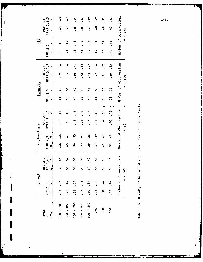
Table 10 presents the results. Some conclusions are: 1) The subset

which includes just straight flow generally shows considerable increases in

explained variance over the full data set. 2) In the cyclonic and anticy-

clonic cases, only estimation of the u-components generally shows improve-

ment due to stratification. This would be expected from the gradient-wind

equation. 3) Generally, there was considerable improvement.

We therefore performed a test to see whether the differences in the

equations were physically reasonable. In particular, the anticyclonic equation

should yield stronger winds and wind shears for the same input than the equa-

tions for straight flow. However, this did not turn out to be the case, so

that the anticyclonic equations are probably not reliable.

thttereibe

t-. -T r- as CNI mN C*.4 -42-

C-,

4 I

en r,- ' ' r-4 r-4 C'J

> . . T e I T en~ a' ,- n c' ,

.4C1 .4 .4 .

S C C. .* Z

C, LC 0 '0 L1 4 ' . .0 0

CN L(n C) C14 en~ r. -4 C) >CJu/l U0 '0% L(n -T .0 . Lfn Lfn 1.

4-4I

10 0scn > Ln L

-4 .n IT .T .T

4',

C C-I '0 ui CO -4 . C pCO~i~ LI '. 4' '.0 .4 f~ Li . -W

4- 0C

011

:D %0 Ln ~'~ .

en~f 0'. '.0 ID 1-4 .4 .4 0- C i.C-T) Ln' M- LI') U Lfl Lf) IT 0- C

C14 -H

a)0 0

cn~~4 IT mIT V

C~ Cr LII U CC'- co C'- co C

CC

rnI

-43-

In contrast, comparison between the equations for cyclonic and straight

flow suggested reasonable behavior of the respective equatins.

In this experiment, we estimated mean wind shear and wind components from

means of MSU 2 and 3 radiance gradients. In all cases, the predicted values

were less in the cyclonic than the straight-contour sample.

7. Summary and Conclusions

This report is a pilot study, based on data from March 1979. Regression

equations were developed and tested which led to estimates of winds and

vertical wind shears, given horizontal gradients of radiances in various

infrared and microwave channels. Due to the small sample, the results must

be considered highly tentative.

The project suggests these conclusions:

1) In spite of their slightly better vertical resolutions, infrared

radiance gradients show very little skill for estimation of synoptic-scale

wind shears centered in the middle troposphere. Microwave gradients are con-

sistently superior, and the improvement due to addition of infrared informa-

tion may not be statistically.significant. Therefore, and because microwaves

are relatively insensitive to clouds, we recommend that large-scale wind

properties be estimated on the basis of microwave radiance gradients only.

Infrare! data should be used only in areas of limited cloudiness.

2) Without stratification by curvature of the flow, radiance gradients

can account for about 50% of the variances of the shears in the middle tropo-

9 sphere (e.g., 300 mb to 850 mb), provided the observations are smoothed. A

very limited experiment suggests that these variances can be increased to 60%

if curvature and infrared channels are included. Standard errors of estimate

for some of the results should be reduciblc to 15 knots or loqcz.II

-44-

3) The regression equations performed almost as well on the winds them-

selves as on wind shears. However, if we base the verification on smoothed

fields, shear estimations are improved more than wind estimatiox,.

4) The weights derived statistically have physically reasonable signs.

5) It is not clear whether the results are satisfactory for practical

use. Such a decision requires comparison of the accuracy of statistical

techniques with that of physical techniques.

S. Suggestions for 1-uture Work

The results discussed here are tentative, because of the small sample

involved. A significantly larger sample is needed to test the practical

utility of the regression techniques.

On this larger sample, the following tests are suggested.

1) Test infrared and microwave predictors always in the same common

periods, in areas of few clouds only.

2) Test the equations primarily on smoothed observations (although

they must be derived from unsmoothed observations).

3) Handle curvature by developing equations between curvature effect

and errors of the equations derived without allowing for curvature.

4) Test all equations on an independent sample.

5) Compare the standard errors of statistical techniques with standard

errors of physical techniques, on the same set of data.

I-45-

REFERENCES

Brodrick, H. J., 1978: The relationship between vertical sounder

radiances and mid latitude 300 mb flow patterns. J. Appl. Meteor.

17, 477-481

Brodrick, H. J., 1980: Structure of a baroclinic zone using Tiros-

N retrievals. Preprint Vol., Eighth Conf. on Wea. Forecating

and Anal. Denver, Co. 129-134.

Carle, W. E., and J. R. Scoggins 1981: Determination of wind fromNimbus 6 satellite sounding data. NASA Reference Publication1072. Texas A & M Univ. College Station, TX. 72 pp.

Cressman, G. P., 1959: An operational objective analysis system.Mon. Wea. Rev. 87, 367-374.

Douglass, A. R. and J. L. Stanford, 1980: The relationship between

the gradient of satellite-derived radiance and upper tropospheric/lower stratospheric winds. J, Appl. Meteor. 19, 113-115.

Fleming, H. E., 1979: "Determination of vertical wind shear fromlinear combinations of satellite radiance gradients: A theoretical

study". United States Naval Postgraduate School, 42 pp.

Kidwell, K., 1979: "NOAA Polar Orbiter Data (Tiros-N) Users Guide".The Satellite Data Services Division.

Lee, D. H., 1979: Level assignment in the assimilation of cloud motionvectors. Mon. Wea. Rev. 107, 1055-1074.

Lorenz, E. N., 1977: An experiment in nonlinear statistical weatherforecasting. Mon. Wea. Rev. 105, 590-602.

Phillips, N. A., et al., 1979: An evaluation of early operational

temperature sounding from Tiros-N. Bull. Am. Meteorol. Soc.

60, 1188-1197.

Phillips, N. A., 1980: Two examples of satellite temperature retrievals

in the North Pacific. Bull. Am. Meteor. Soc. 61, 712-717.

Sampson, R. J., 1978: "Surface II Graphics System". The Kansas

Geological Survey, 240 pp.

-46-

REFERENCES (Continued)

Smith W. L. and H. M. Woolf, 1976: The use of eigenvectors of statisticalcovariance matrices for interpreting satellite sounding radiometerobservations. J. Atm. Sci. 33, 1127-1140.

Smith, W. L., et al, 1979: The Tiros-N operational vertical sounder.Bull. Amer. Meteor. Soc. 60, 1177-1187.

Zak, J. A., 1967: Estimation of wind in the stratosphere from satelliteradiation at 15 microns. M.S. Thesis. Pennsylvania State University.

Zak, J. A., and H. A. Panofsky, 1968: Estimation of stratospheric flowfrom satellite 15-micron radiation. J. Appl. Meteor. 7, 136-140.

I

II

I

I-47-

APPENDIX A: FURTHER DETAILS ON TIROS-N RADIANCE DATA PROCESSING

The TOVS System

The new generation NOAA polar orbiter satellite system contains an

instrument package which includes an Advanced Very High Resolution Radiometer

and the TOVS. The TOVS system includes three sensors, namely the High

Resolution Infrared Radiation Sounder (HIRS/2), the Microwave Sounding Unit

(MSU), and the Stratospheric Sounding Unit (SSU). A fourth sensor, a

backscatter ultraviolet system for ozone measurement, is expected to be

added later in the satellite series. Each sensor is a multi-channel

radiometer which measures the radiation emerging from the top of the

atmosphere. Only the HIRS/2 and MSU data were used in th research discussed

in this paper.

The HIRS/2 instrument measures the incident atmospheric radiation in 19

regions of the infrared and one region of the visible part of the spectrum.

The three HIRS channels used in this research were channe'q 3, 4 an 5 which

correspond to central wavelengths of 14.5, 14.2, and 14.0 pm respectively.

These channels in the 15 wm band provide better sensitivity to the temperature

of relatively cold regions of the atmosphere than can be achieved with the 4.3

Pm HIRS band channels. Channel 5 radiance values are also used to calculate

the heights and amount of cloudiness within the HIRS field of view. The

instantaneous fields of view (IFOV) of the HIRS/2 channels are stepped across

the satellite track by use of a rotating mirror. This cross-track scan,

which covers a linear dimension of about 2240 km, combines with the satellite's

motion in orbit to provide coverage over a major portion of the Earth during

any 24 hour period. Each individual HIRS/2 measurement (scan spot) results

from a 17.4 km diameter circular area at the subsatellite point expanding to

approximately a 30x60 km ellipse at larger scan angles. Fifty-six scan

m I

-48-

spots comprise one scan line, which is achieved by each mirror rotation. A

sounding is then extracted for every array of seven scan lines and nine

scan spots through a weighting technique. The result is a 5 x 6 array of

data for each 40 x 56 array of scan spots. A calibration every 256 seconds

(40 mirror rotations) replaces the measurements for 3 scan lines causing a

larger than normal spacing between data at the end of the 256 second period.

Thus, the along track data points are arranged in a series of 5 points about

250 km apart, with roughly a 35% greater spacing between the groups of five.

The MSU sensor is a passive scanning microwave spectrometer with 4

channels in the 5.5 micrometer region of the spectrum. The two channels used

in this research (channels 2 and 3) respond to 53.74 and 54.96 GHz frequencies.

The microwave channels probe through clouds and are used to negate the

influence of clouds on the 4.3 pm and 15 Pm HIRS channels. The MSU has a

wider FOV than the HIRS, accounting for only eleven FOV along its 2240 km

swath. MSU soundings are extracted in a similar fashion to that used for

the HIRS with the MSU measurements interpolated to the HIRS scan positions

hence constituting a similar grid as the HIRS.

Data Processing

The transformation of radiances measured in the 24 spectral intervals

of the TOVS system (20 HIRS, 4 MSU) into vertical profiles of atmospheric

temperature is accomplished through the operation of 4 principal software

modules on an IBM 360/195 computer system. A brief discussion of 2 of these

modules, namely the Preprocessor and the Tiros Atmospheric Radiance Module

(TARM) follows.

The Preprocessor organizes the output of the TOVS data into a form which

is convenient for scientific processing. Input to this module consists of

!1

-49-

time coincident sets of HIRS and MSU measurements with earth location and

calibration equations appended. These data are representative of the

radiation emitted from the top of the atmosphere.

The major function of TARM is to transform the individual FOV data

provided by the Preprocessor into sets of atmospheric radiances for determin-

ation of atmospheric parameters by the Tiros Retrieval Module (TRET).

The Preprocessor output for both the HIRS and MSU data is organized to

allow formation of boxes whose dimensions are 9 scan spots across the satellite

track by 7 scan spots along the track. Subsequent operations performed

within TARM are in terms of these FOV ensembles. These operations aim to

produce a single set of radiances in the 24 spectral intervals of HIRS and

MSU, from which an atmospheric sounding can be obtained in TRET.

The physical problem addressed in TARM is the extraction of the true

thermal emission of the atmosphere within the volume being sampled from

the collection of radiance measurements. Since there are likely to be clouds

over such a region and since up to 50% of the HIRS spectral measurpmen.L

in channel 3,for example, are subject to contamination by clouds, this

endeavor is known as the clear column radiance problem. This cloud con-

tamination occurs in HIRS channels which have weighting function peaks in

the mid-troposphere where clouds greatly affect radiance measurements.

There are two basic approaches to the clear column radiance problem.

First, an attempt is made to find holes in the clouds where uncontaminated

observations can be obtained. Second, statistical techniques can be applied

in order to infer clear column radiances from the contaminated ensemble.

Both methods are utilized in TARM.

Initially, the observations for each FOV in a box are given objective

tests to determine the probable presence of clouds. These tests, which are

,i |

-50-

related only indirectly to cloud amount, involve comparison of the measured

reflectance with the expected surface albedo, longwave and shortwave window

channel comparisons, longwave window brightness temperature and expected

surface temperature comparisons and an infrared-based regression estimate

of the microwave brightness temperature and the observed microwave brightness

temperature. The expected surface temperature is obtained from analyses of

ships and satellite sea surface temperatures as well as shelter land

temperatures. Since the vertical weighting functions of several tropospheric-

sensing HIRS channels bracket those of the MSU channels, the regression test

gives physical reasoning to expect accuracy in predicting the HIRS radiance

from MSU measurements in the absence of clouds. However, in the presence of

clouds, the HIRS predicted MSU radiance will be too low.

A box is considered to be clear if as few as 4 of the 63 FOVs are found

to be clear. The clear value for each of the parameters associated with the

box is a weighted average over the clear FOVs. In the event that fewer than

four clear FOVs are found in the initial search, a second approach, the so-

called adjacent pair or N* technique is employed.

The specification of "cloud-free" infrared radiances from cloud-

contaminated observations is performed by using the "paired field of view"

method. This technique assumes that the variation of radiance observed in

two neighboring fields of view is caused explicitly by a variation of

cloud amount. In this situation the cloud free radiance R. is given by

R.= Rlj NR2j ()J i -N*

I!-51-

where the subscript j refers to the spectral channel and the numerical

subscripts refer to the two geographical fields of view. The parameter N*

is the ratio of cloud amounts, NI/N2, in the two fields of view. For the

Tiros N, it is desirable to make use of the radiance observed in microwave

channels, which'penetrate clouds, in the specification of clear-column

infrared radiances. Through the use of radiance eigenvectors, a simultaneous

equation for N* can be obtained and the clear column radiances of all channels

can also be obtained as functions of the radiances observed in all

channels, infrared and microwave.

The use of these eigenvectors produces solutions that are optimal for the

number of parameters used in a statistical sense.

The minimum number of acceptable pairs for N* success is four. The

output is a weighted average, with the weight for each pair being proportional

to the reciprocal of the error in the regression estimate of the MSU bright-

ness temperature based upon the HIRS clear column radiance determination.

In the event that both the clear search and the adjacent pair method

fail, the output for the 63 FOV box is taken as a spatial average of the MSU

channels and the stratospheric based HIRS channels (i.e., those presumed

not subject to cloud contamination).

The final result is a grid encompassing the North American continent

with radiances covering the network (grid) at a horizontal resolution of

about 250 km.

1

I

I

' ..,, L , , z, -L

-52-

APPENDIX B: SINGLE CHANNEL MAPPINGS FROM THE DEVELOPMENTAL SAMPLE

This is a selection of single channel radiance maps drawn for the 21-

day developmental sample. The purpose of the inclusion of this set of maps

is two-fold.

1) Maps of radiance contours with raw radiance values plotted are

included to give the reader a feeling for the density and distribution of

observations in the five channels used. The maps presented here are from

relatively data rich days. Even on these data rich days,gaps in the data

are evident especially for HIRS 5 whose peak energy contribution comes from

the middle troposphere. It's sensitivity to clouds is thus apparent.

While the number of observations in HIRS channels 3 and 4 is somewhat better,

the gradients are much weaker renderiag their information less useful.

2) Maps of radiance contours with shear arrows are included to supple-

ment the maps in the body of the text. These show additional examples of

the correspondence between radiance gradients in various channels with wind

shear in the middle troposphere. It is interesting to note that in the maps

presented here,cross contour departures appear to be most prevalent on the

eastern part of the maps. This may be partially accounted for by the fact

that time correspondence between radiance observation and wind shear obser-

vations is poorest in these locations. Thus, especially with rapidly

translating systems, systematic departures here may be expected.

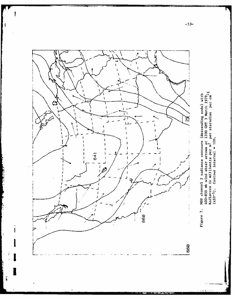
4 -53-

C\E! 4 Scd

U) 0

w o CN-.0 E.lc0-~ W 1

413

0

ca

z(0

ca u= Lf)r- I.

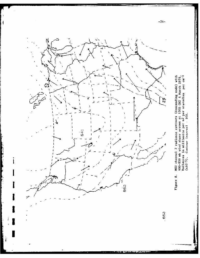
-54-

\ •\ 5

-

_0 '4 $w

*~~~Z c .- o*

'4 ,* - -.-

( r• K .J - ,N j ,

$} CO C

0 EO, . I I : c1

0 0

0

I- S. C ' -H

I- i... ..

V)co -( 0 I / - 0)

• " I,_*- // -I. I, -, "0G J"

/'I/ I ".- C.Oz,.I

.,- c

/ CO!" I , ,' / l- t 00r/

I, . - I .-.. /r, < _ -. , / ,..,. c a ,

u 0 t 10._,/ 2=I- ,; 7''l./, / uc I

i- . . " " I - I - -l

" II/.r I , /

! - ~-

IN3, (0

I

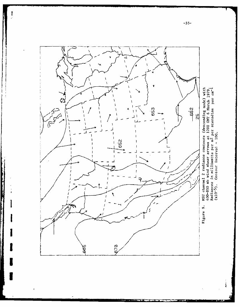
-55-

-.4w

4JJ

~,0 $- .0)

$4 >

o W 1 c

I-40

tt0 C10 cr- '

10 H

E corIaca

_ _ _ _ _ _LfI____ ___ -4C-InC

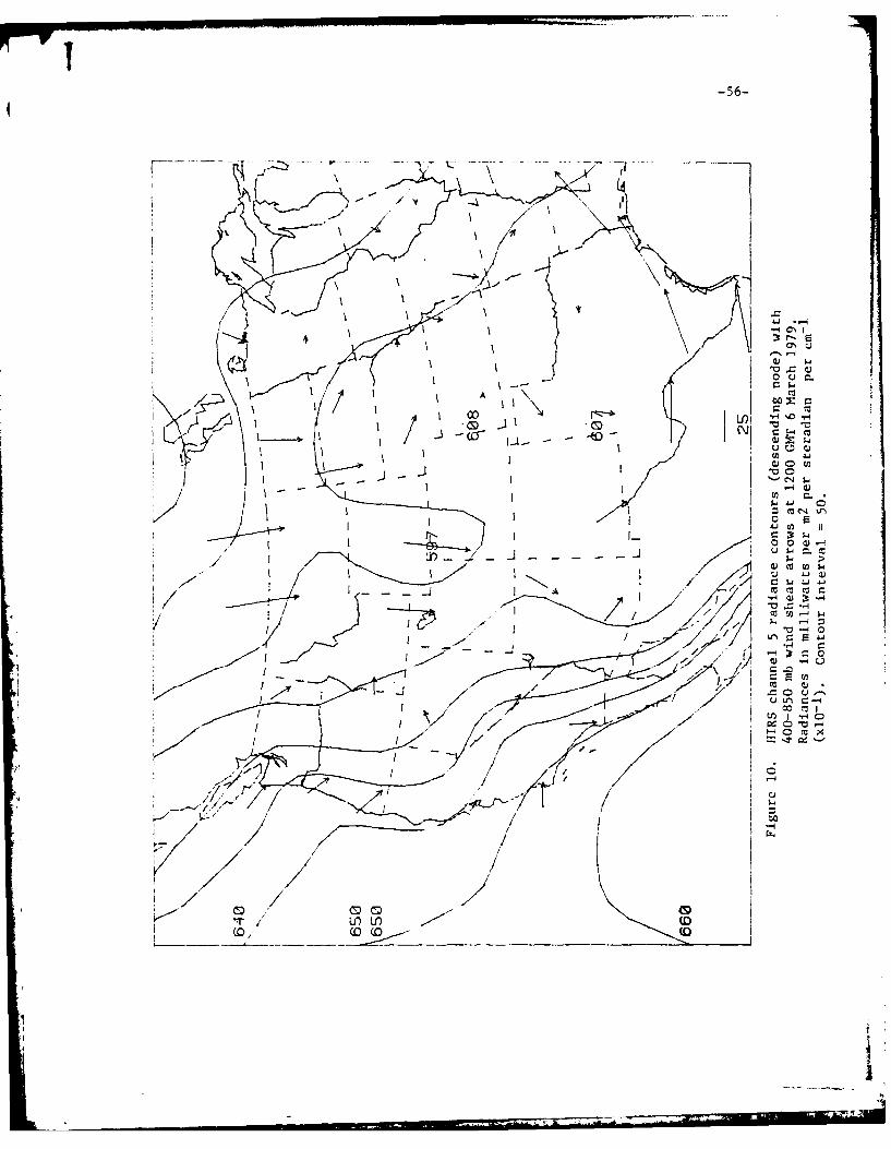
-56-

H. as I

a

JJ 0.

CLD -4 S .

-~c IcJI4 U')Oto~

vio

00 m.. I

1r UlLO(

co 5D(C

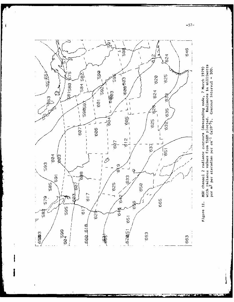
4 -57-

Lr cli 10U'))

(D (

(0

r. 0

I~~~ ,- cr Y)-

"a00

c~com C) (0A (Y(0

MI c

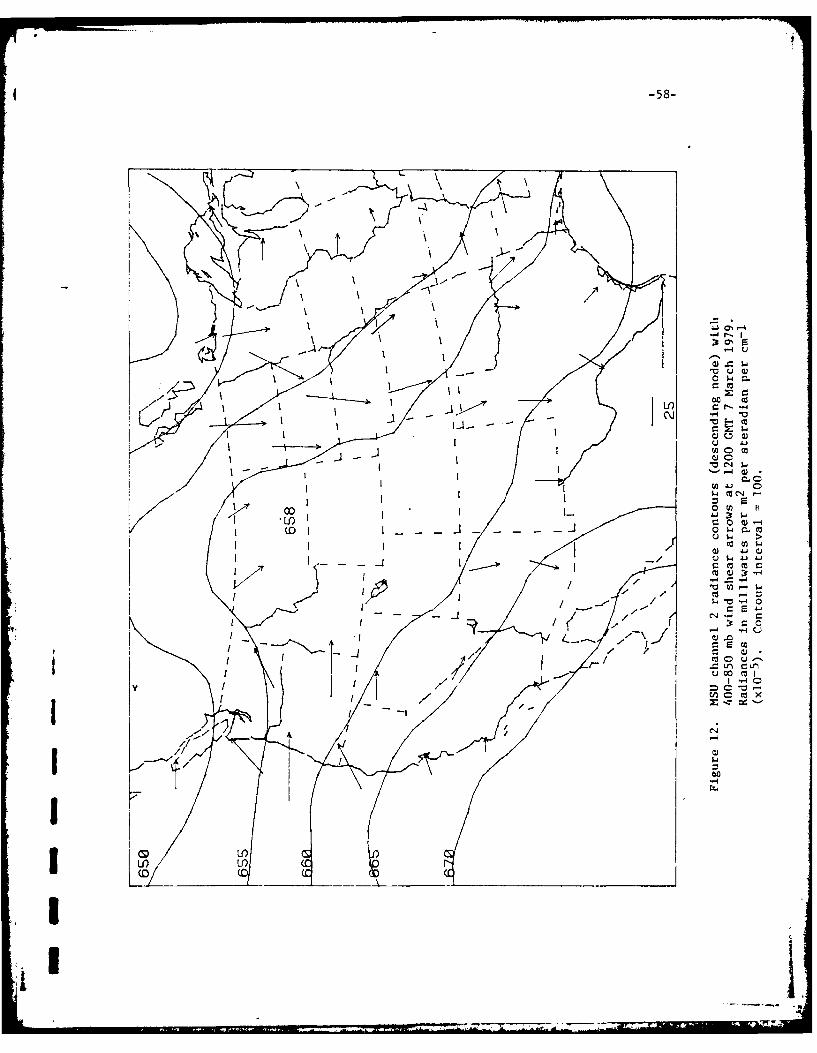
A -58-

.- 4 C)

cu w0 o

JC,'V C'J $4

o C14 -4

OD~C 0 w U

U 14 >~

Ij $4 4 0

(A~ C~ xX:~ --T

CNJ

LIO

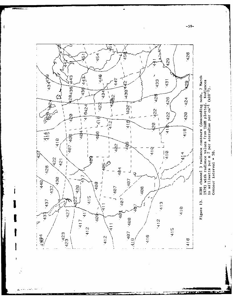
4-.59-

N C

c- N

N N co- x

' -e

N E- - .

a -W 44- N-

= >-

7~ co L

-,4 )irN flU u~ 1

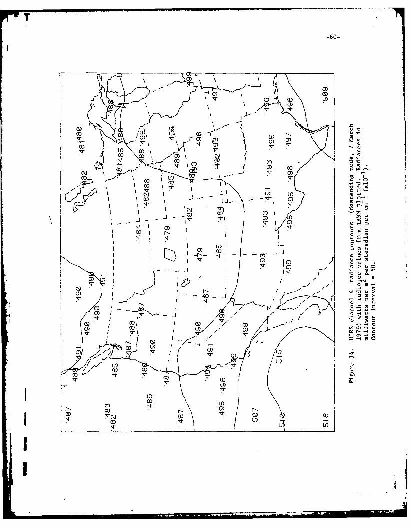
-60-

- - ~O 1a 0)

( ( 0 (D )

0 I

co L LU) I. .Ol0) C") 0)Ix'~

0) %o O 0)0* ~0 ) 4- 0

co I r 0) 0 0-

- 0)

4- C J-4

41-4

oY cc U 1

C41 -1

0)C'IT 0

(5) H-- N C'4

oo k- 0 000 -H . -~ 4

'IT 0)

Co Lio

K 0000 'TJ 00CD 0

0C O

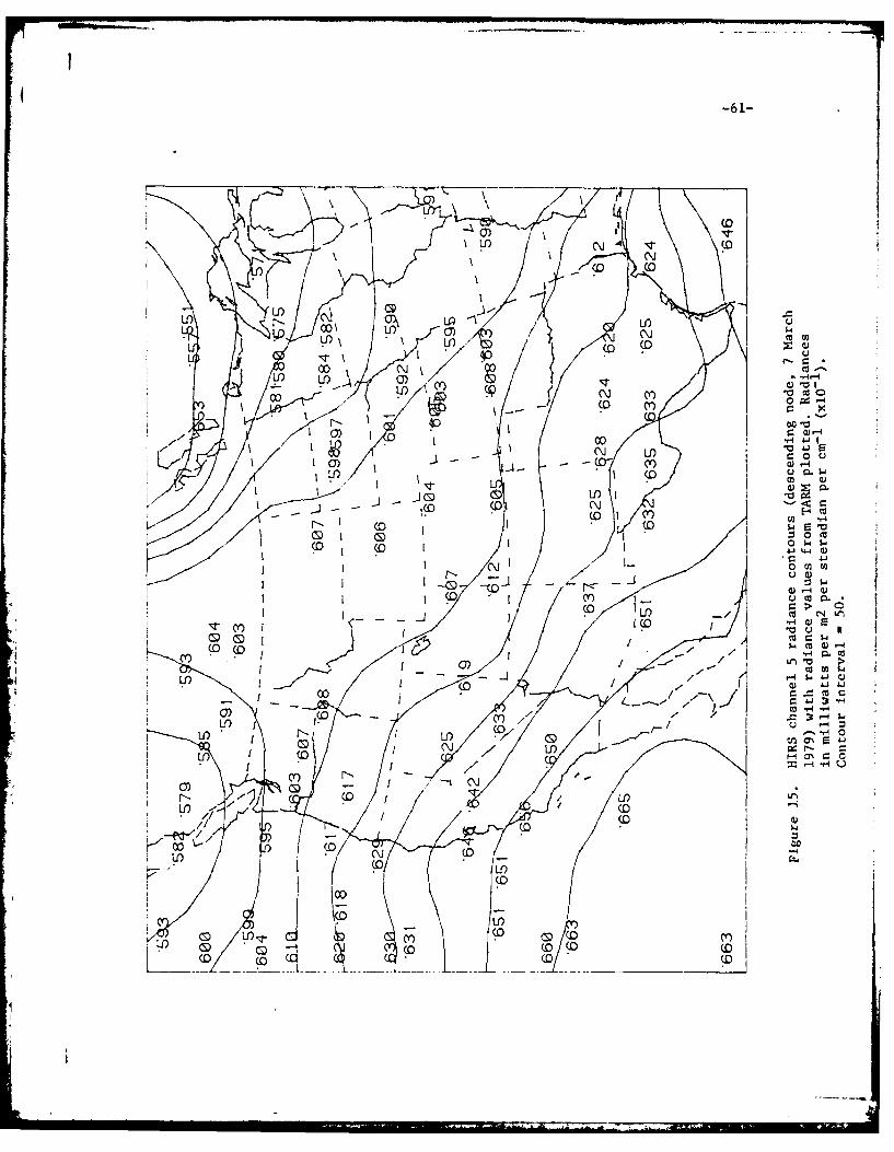
0L)

II \

U) 001 L

U ~ U) G) 0

U) U

LO 10) a) .-V

Nn U)"

-r 0-C(0f 1i -4

I ~ Ip

(0 (0

(D 0 W 4

U)Y

r-.,- c0

0))cLOi

U-Q00C c

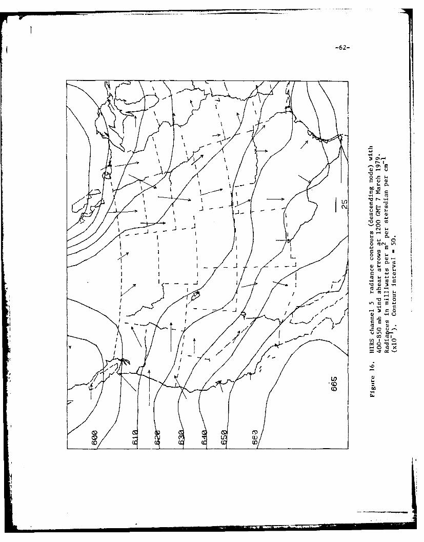
4 -62-

Iu . -4 Q*

0 w0

to m- c

,w

-0 C" U'

-4

.- 4

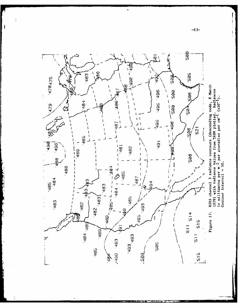
-63-

7-

0)) (0

U) 00WCUr)

CD

a;~ "Co

00 "0 -4)1-1

Iu mICS L Ln(

1 00 -CO2.00 t- uU )~ ~~ ~~~.~ 7 '( YL-- . a ) I j4 Co.~. cc

00 $4to a)1-

00 1 r-X ccr__rr__"_3t -4

/0 /t -4Co oa

1 0 0 rz .6

M~ jo c

LL

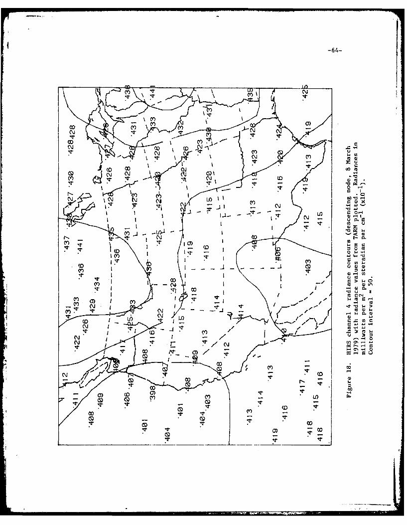
4 -64-

ccrJ

00- (0 -NV

00- 00C~~rJ I' a)1

cr .04

0))(N 7\ 7l

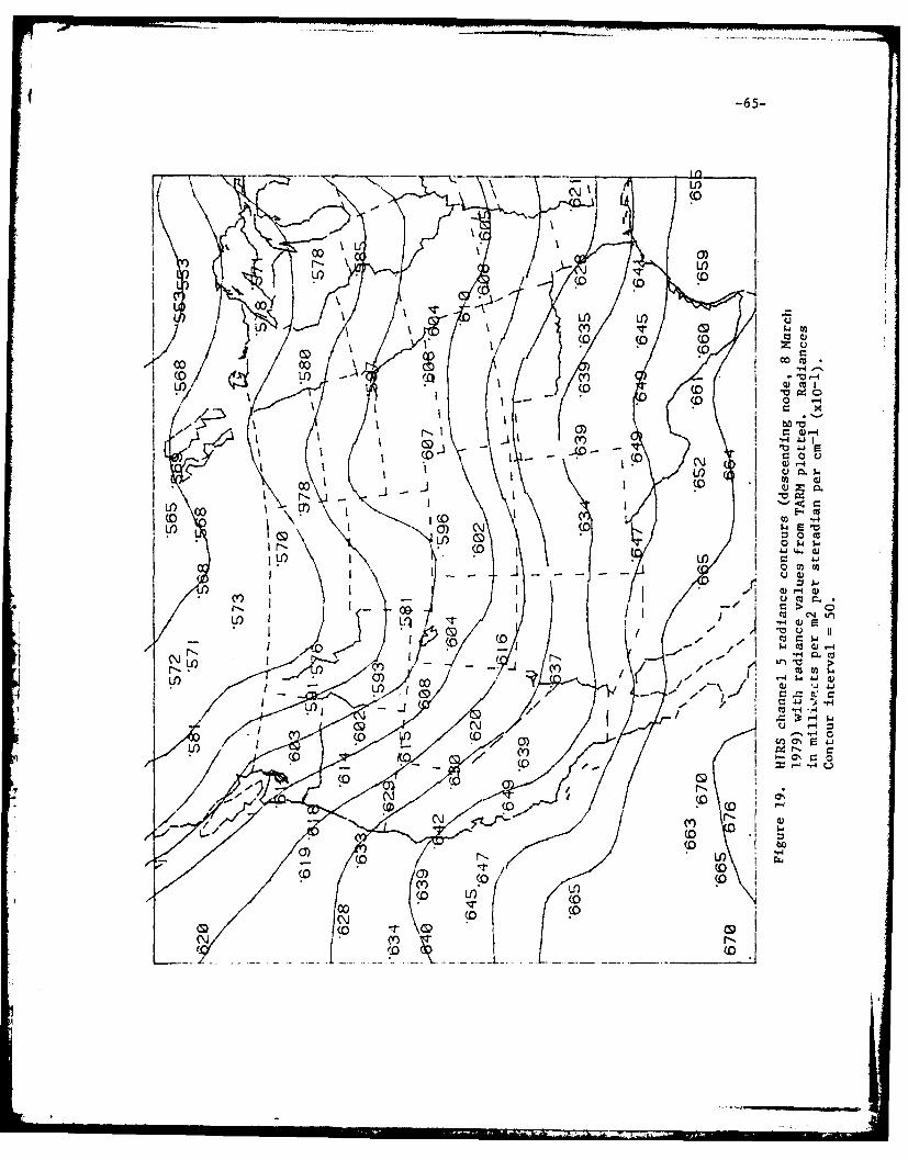
-65-

(0

(0 (Dc~

Ln~ co T

(0 (0

-4SO

(Y(0

LI)

(0

Documents

EhmhmhhhmD - apps.dtic.mil