European Historical Economics Society

EHES Working Paper | No. 217 | October 2021

China, Europe, and the Great Divergence: Further Concerns about the Historical GDP Estimates for

China

Peter M. Solar, CEREC, Université Saint-Louis - Bruxelles and

Faculty of History, University of Oxford

EHES Working Paper | No. 217 | October 2021

China, Europe, and the Great Divergence: Further Concerns

about the Historical GDP Estimates for China*

Peter M. Solar, CEREC, Université Saint-Louis - Bruxelles and Faculty of History,

University of Oxford

Abstract

Broadberry, Guan and Li (2018) made estimates for China’s GDP per capita from 980 to 1840 in order to date the onset of the Great Divergence between China and western European economies. In response to Solar’s (2021) criticisms, they (2021) made some revisions to the estimates but largely dismissed most of Solar’s concerns, particularly those about their series for China’s population and its implications for dating the Great Divergence. This working paper assesses their revisions, reaffirms concerns about the level of their 1840 benchmark, and points out the weaknesses of the population figures in greater detail. The dating of the Great Divergence turns out to depend on the population series used and on the interpretation of what was happening to incomes in China during the mid-seventeenth century. This paper recommends considerable skepticism about Broadberry, Guan and Li’s estimates.

JEL Codes: E01, N15, O47, O53

Keywords: China, Great Divergence, historical national accounts, population

Notice

The material presented in the EHES Working Paper Series is property of the author(s) and should be quoted as such. The views expressed in this Paper are those of the author(s) and do not necessarily represent the views of the EHES or

its members

1Corresponding Author: Peter M. Solar, (psolar@vub.ac.be)

*I would like to thank Kent Deng, Ye Ma, Kim Oosterlinck, Cormac Ó Gráda and Bas van Leeuwen for helpful comments on drafts of this working paper and Ye Ma and Bas van Leeuwen for sharing data underlying their own estimates of China’s historical GDP. I am also grateful for advance sight of several chapters from the forthcoming Cambridge Economic History of China.

1

Developments in China, the world’s largest economy in the pre-industrial era, are central to the

debate about when countries in western Europe and north America opened a widening

economic gap with respect to the rest of the world. By the mid-nineteenth century the gap was

evident, both economically and politically, but there has been considerable debate about when

divergence started and, as a result, whether the poor became poorer because the rich became

richer. Various sorts of evidence have been invoked to pin down the dating of the divergence.

Pomeranz (2000), for example, compared consumption per capita of key goods, while Allen et

al. (2011) looked at real wages. In a recent paper Broadberry, Guan and Li (2018; hereinafter

BGL) have argued that such sorts of evidence refer only to particular places and are only

partial indicators of economic performance and that historical national income accounting

provides a superior method. They make estimates for the China’s GDP and GDP per capita

back as far as 980 and compare them to existing estimates of GDP per capita for leading

western European countries. The Great Divergence, according to their results, began c.1700

and involved both rising incomes in the west and falling incomes in China. This dating was

earlier than that proposed by Pomeranz, who favoured the late eighteenth century. Allen et al.

found that real wages in England in the mid-eighteenth century were already much higher than

in China and other parts of Asia, before further divergence from around 1800.

Solar (2021) pointed out several problems with BGL’s estimates. First, they were constructed,

for over 90 per cent, on two series, those for grain output and population. Second, despite its

small weight in the estimates, the government sector, as estimated, implied that it amounted to

more than 30 per cent of GDP c.1400, an implausibly high level, particularly given what is

known about tax revenues. Third, BGL’s 1840 benchmark, the anchor for the entire series of

estimates, was not firmly based and was too high when compared with two other sets of

estimates for China’s GDP around that date. Fourth, plausible revision of the government

sector left a very sharp peak in GDP per capita c.1700, of which Solar found no echo in the

English-language historiography of the period. Solar suggested that this peak may have been,

at least in part, an artifact of the series for population used by BGL and pointed out that it

raised a problem in dating the beginning of the Great Divergence.

In response to these criticisms, BGL produced a “restatement” (2021) in which they conceded

that there was indeed a problem with the government sector, but essentially dismissed or did

2

not address Solar’s other points. They produced a revised series for the government sector, as

well as reducing this sector’s share in GDP at the benchmark year. In addition, they revised

their series for grain output upward during the Ming dynasty (hereafter abbreviated to Ming).

These changes fed into a new set of estimates for China’s GDP and GDP per capita from 980

to 1840.

BGL’s revised estimates still beg many of the same questions raised in Solar’s comment.

Before the revised estimates and the interpretation that BGL put on them become fixed in the

literature and their numbers used indiscriminately by scholars not intimately familiar with the

way in which they were constructed, it is important that they be thoroughly tested. With the

comment by Solar and the restatement by BGL, the editors of the Journal of Economic History

decided to close discussion in the pages of that journal, so this working paper continues the

debate. Since Solar, who does not read Chinese, has only very limited access to the Chinese-

language literature and sources, it is hoped that these exchanges will stimulate historians of the

Northern Song (960-1127 AD), Ming (1368-1644 AD) and Qing (1644-1912 AD) economies

to cast a critical eye on BGL’s estimates.

The issues in question and their significance for China’s GDP per capita are captured in Figure

1, where BGL’s initial and revised estimates are shown along with estimates by Xu et al (2015,

2017) and by Ma and de Jong (2019). Solar’s comment experimented with various

assumptions about the government sector—for example, that its share remained constant over

the entire period or that government expenditure per capita remained constant—and concluded

that GDP per capita during the early Ming might have been at least 20 per cent and even

perhaps 30 per cent lower during the Ming. BGL’s revisions mainly affect both the Northern

Song and Ming periods and involve a significant reduction, of up to 20 per cent, in estimated

GDP per capita during the Ming. As a result, the early Ming no longer seems to have been as

prosperous as the Northern Song at its peak (c.1050 CE) and, instead of incomes falling off

during the Ming, there are only fluctuations around a stagnant level. The revisions also make

the decline in per capita incomes during the late Northern Song much more pronounced. So

one set of questions is: What was the nature of BGL’s revisions? Were they appropriate?

Were they sufficient?

The estimates by Xu et al and by Ma and de Jong, like BGL’s in 1990 international dollars, are

both 10-12 per cent lower than BGL’s. Solar suggested that these other estimates were more

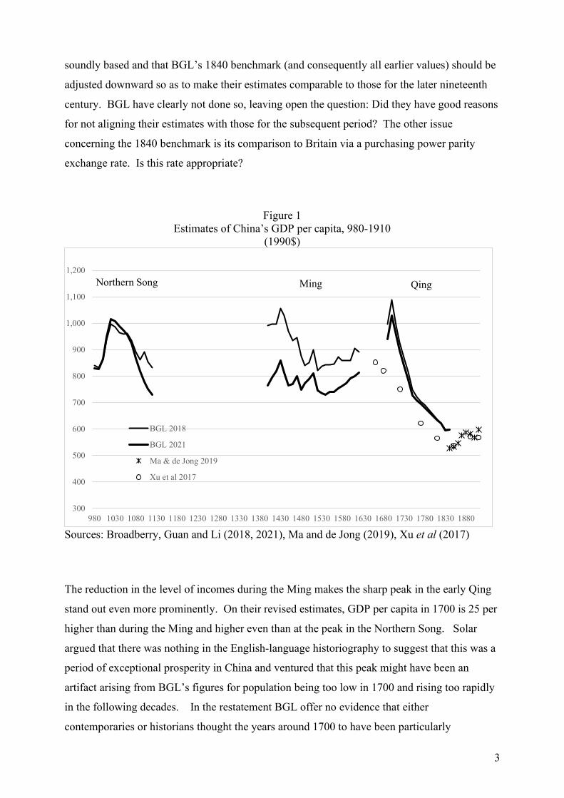
3

soundly based and that BGL’s 1840 benchmark (and consequently all earlier values) should be

adjusted downward so as to make their estimates comparable to those for the later nineteenth

century. BGL have clearly not done so, leaving open the question: Did they have good reasons

for not aligning their estimates with those for the subsequent period? The other issue

concerning the 1840 benchmark is its comparison to Britain via a purchasing power parity

exchange rate. Is this rate appropriate?

Figure 1

Estimates of China’s GDP per capita, 980-1910 (1990$)

Sources: Broadberry, Guan and Li (2018, 2021), Ma and de Jong (2019), Xu et al (2017) The reduction in the level of incomes during the Ming makes the sharp peak in the early Qing

stand out even more prominently. On their revised estimates, GDP per capita in 1700 is 25 per

higher than during the Ming and higher even than at the peak in the Northern Song. Solar

argued that there was nothing in the English-language historiography to suggest that this was a

period of exceptional prosperity in China and ventured that this peak might have been an

artifact arising from BGL’s figures for population being too low in 1700 and rising too rapidly

in the following decades. In the restatement BGL offer no evidence that either

contemporaries or historians thought the years around 1700 to have been particularly

300

400

500

600

700

800

900

1,000

1,100

1,200

980 1030 1080 1130 1180 1230 1280 1330 1380 1430 1480 1530 1580 1630 1680 1730 1780 1830 1880

BGL 2018

BGL 2021

Ma & de Jong 2019

Xu et al 2017

Northern Song Ming Qing

4

prosperous and persist in their assertion that, as for the population figures, there were “only

small differences between our estimates and those of other scholars” (p. 966). Were these

differences so small? What impact might they have on the estimates for GDP per capita

c.1700? For the dating of the Great Divergence?

In the following sections the questions raised in the previous paragraphs will be taken up in the

same order. Then the implications of a set of “guesstimates” for dating the Great Divergence

will be considered. The working paper finishes with short comments on BGL’s use of

subjective error margins, the difficulties of replicating their work, and the need for it to be

thoroughly assessed by scholars more familiar with the sources for the Northern Song, Ming

and Qing periods.

Revising the Government Sector

BGL acknowledge that their estimates for the government sector, particularly during the Ming,

were far too high. The only indication of what went wrong comes when they state that

“Unfortunately, the data that we used from the Ming shilu and Wanli Kualiji also covered other

elements of state spending and therefore recorded too high a level of expenditure in the Ming”

(p. 959). They do not tell us what this other state spending comprised nor why it should not be

counted as government expenditure. Readers deserve to know more precisely what it was that

went wrong.

Instead BGL set about dealing with this problem along two lines. One is to revise the way in

which they estimate government spending. In their original article, they multiplied the

numbers of civil servants and soldiers by their salaries for each period, then deflated nominal

expenditures by a price index. In the revision, they use a different method for each dynasty.

For the Northern Song they rely only on the numbers of civil servants and soldiers. For the

Ming they use a share of land tax revenue presumed to represent expenditures, then deflate

these nominal revenues by their price index. For the Qing they retain the original method.

They argue on page 2 that their reliance on the land tax revenues during the Ming “makes the

Ming data broadly comparable with the data for the Northern Song and Qing dynasties, based

only on the pay of soldiers and civil servants” (pp. 959-60), but on the following page they

decide to use the numbers, not the pay, of soldiers and civil servants for the Northern Song.

BGL provide no guidance as to how they linked the numbers of government workers in the

5

Northern Song to the deflated value of land tax revenue in the Ming. (BGL change their

method for the Northern Song because of “the rather rough nature of the price deflator” (p.

960), but do not explain why it is “rougher” in the Northern Song than in the Ming or the

Qing.)

A simpler and more consistent method would have been to use the numbers of civil servants

and soldiers in each period, rather than rely on a GDP deflator composed only of grain and

cloth prices. However, as pointed out in Solar’s comment, the size of the Chinese army is

often difficult to determine. During the Northern Song it had three major components: the

imperial army, the local army and rural troops. Wong (1975) cites figures for the first two

that show growth from 378,000 in the 960s and 970s to 1,258,000 in the 1040s before a decline

to 840,000 in the 1080s.1 The rural troops were a militia, occupied during peacetime with

farming (in such times the local army was used to do public works). Wong’s figures bear no

resemblance to BGL’s new (undocumented) numbers of soldiers and civil servants, which

increase at a constant rate from 445,000 in 980 to 588,000 in 1080.

During the early Ming “military families” were liable for the provision of soldiers, and it is

very often the numbers of these families that were counted rather than effective soldiers. Such

families were allotted “military lands” on which to grow their own food, raising the possibility

that their output would be counted twice, as agricultural production and as government activity

(Robinson 2013). The comment also noted that large numbers of soldiers were employed in

transporting grain along the canals. BGL chose not to consider the issue of double-counting,

particularly in the early Ming, when, even on the revised estimates, the government’s share of

GDP is more than four times higher than in the mid-nineteenth century and more than three

times higher than in the late Northern Song (p. 964). They cite Liu’s (2015) description of the

early Ming as “the largest command economy in the pre-industrial world” (p. 964), but this

should have set off alarm bells for how they estimated output.

The issue of double-counting is particularly pertinent since the other major revision to their

estimates, following Shi, is to increase the amount of cultivated land by 9.2 per cent during the

Ming. Shi (2020, p. 155, n. 2) argues that previous estimates were too low precisely because

they did not include “various parcel of state-owned land at the time, such as those in the

1 Deng and Zheng (2015) cite the same figures for 978 and 1048.

6

possession of the imperial family, princes and other nobles, military land and others” (italics

added).

The other way in which BGL have “solved” the problem of the government sector being too

large in earlier periods is to reduce its share in GDP at their 1840 benchmark from 4.7 per cent

to 2.1 per cent. Since BGL’s revised estimates are extrapolations back from their 1840

benchmark, the lower share of government in GDP does much of the work of bringing Ming

government expenditure back into a more reasonable range, as is shown in Figure 2.

Figure 2 Shares of Government in GDP during the Ming

(per cent)

Notes: “BGL 2018 reduced government share” shows the effect of reducing the benchmark share of government in GDP from 4.74 per cent to 2.13 per cent. “BGL 2021 reduced government share” shows that effect on the revised estimates of eliminating the adjustment to the amount of cultivated land during the Ming. BGL draw this lower share for the government sector from Liu’s (2009) estimates for nominal

GDP in 1840, a source to which, strangely, they make no reference in the original article,

especially since in this article Liu himself made estimates for Chinese GDP between 1600 and

0

5

10

15

20

25

30

35

40

1400 1420 1440 1460 1480 1500 1520 1540 1560 1580 1600 1620

BGL 2018 BGL 2018 reduced government share

BGL 2021 BGL 2021 revised series and increased land

7

1840. They do not use Liu’s other sectoral shares nor do they offer any evidence relating to

the 1840s for why Liu’s government share should be preferred. They argue that share of

government in Chang’s (1962) estimates for the 1880s looks high (in fact, it was even higher,

at 6 per cent; see Table 1 below).2 They compare it to the government share of 2.84 per cent in

the estimates for 1933, yet in their detailed study of the Hua-Lou economy in the 1820s, Li and

van Zanden (2012, p. 967) put the share of government at 6 per cent.

The reason why Chang’s share for the 1880s is so high reveals a major difficulty in putting

numbers on government spending in Qing China. Chang’s estimates were made in the context

of a study of the incomes of the Chinese gentry, which included most public officials. Local

and provincial magistrates transferred most official tax revenues on to the central treasury,

leaving few resources for local public spending or their own remuneration. They made up for

this deficiency by a variety of informal charges, some tipping over into corruption. Chang

(1962, p. 319) reckoned that income from these informal charges amounted to 115 million

taels, far more than the 49 million taels for the official salaries of civil servants, soldiers and

militiamen. Others have put informal revenues at from 30 to 100 per cent of formal revenue, a

lower but still significant level for the government spending that is difficult to observe (Ma

2011, pp. 31-32; Hao and Liu 2020, p. 921).

The Level of the 1840 Benchmark

In reducing the share of the government sector at the 1840 benchmark, BGL launch the

following attack on Solar for describing this benchmark as an extrapolation from Chang’s

estimates of GDP in the 1880s:

It should be emphasized that although the shares of industry and services in our

benchmark are taken from a study by Zhang (1987) [Chang 1962] for the 1880s, the

nominal GDP in 1840 is anchored in the value of agricultural output derived from

crop output and prices for that year. Solar is, therefore, wrong to state that our 1840

benchmark is based on an extrapolation from the 1880s to 1840 using only a series

for grain output (p. 961).

2 BGL cite Zhang (1987), but this is just a translation into Chinese of Chang (1962).

8

In fact, the only error made by Solar was to write “grain output” instead of the “value of net

grain output”, which is what BGL’s working paper (2017) shows that they calculated. The

working paper also states that “The net output of cash crops is set at 25.2 per cent of the net

output of grain crops, in line with the ratio for the 1880s from Zhang” and “The net output of

livestock, forestry and fishing is set at 10.4 per cent of the net output of grain crops, in line

with the ratio for the 1880s from Zhang” (BGL 2017, p. 50). 3 BGL might thus have more

accurately described their anchor as the “value of net grain output” rather than the “value of net

agricultural output”. As for the rest of output, BGL (2018) state that “The absolute level of

GDP in 1840 is established by first calculating value added in agriculture for that year, and

then applying the shares from the 1880s to calculate the nominal value added in industry and

services” (p. 976). Since Chang calculated the value of net grain output in a manner similar to

BGL’s, BGL would seem to be using the value of net grain output in 1840 to estimate the

values of output in all other sectors of the economy in 1840 on the assumption that in 1840 the

values of output in these other sectors remained in the same ratio to the value of net grain

output as they were in the 1880s. If it walks like an extrapolation…

The net value of grain output is thus the only information from 1840 on which the level of

Chinese GDP is fixed for that year. Since the level of GDP at this benchmark determines the

level of GDP for all value extrapolated back to 980, it is important to get this level right.

Moreover, if BGL’s estimates are to be useful in interpreting Chinese economic growth over

the even longer term, including the period after 1840, then their benchmark for 1840 needs to

be consistent with estimates for later years. All of this seems sensible, yet when Solar

suggested reducing this benchmark by about 11 per cent to bring it into line with the mid-

nineteenth-century estimates by Xu et al (2015, 2017) and by Ma and de Jong (2019), BGL

responded that “having chided us for projecting back from the 1880s to 1840 for our

benchmark, Solar now makes use of an 1850 benchmark which has been obtained by

projecting back from Ma and de Jong’s (2019) benchmark for 1912” (p. 966). They do

acknowledge, in a footnote, that Xu et al’s estimate is indeed much the same as Ma and de

Jong’s.

Their response on this point is a gross misrepresentation both of what Solar did and of Ma and

de Jong’s work. Solar did not make any sort of projection; he simply took values for 1840 and

3 In fact, these shares, as well as the breakdown of grain crops, were not based on information for the 1880s; they were taken by Zhang from work on Chinese agriculture in the 1930s (Chang 1962, pp. 302-3).

9

1850 from the last column in Ma and de Jong’s Appendix Table 4, which presents annual

estimates of Chinese GDP per capita in 1990 international dollars from 1840 to 1912. Nor do

Ma and de Jong’s estimates involve projection backward from 1912. BGL seem to be referring

to their use of a 1912 comparison of Chinese and UK GDP made in order to fix the PPP

exchange rate needed to convert yuan to the international dollar. Ma and de Jong’s estimates

are, in fact, based on annual indicators for the output of grain and of other components of the

agricultural, industrial and service sectors, guided in part by benchmark observations of the

sectoral distribution of nominal GDP in 1840 from Liu, in the 1880s by Zhang and in 1920 by

Xu and Wu. They are thus based on much more information for the 1840s and subsequent

years than is the benchmark value used by BGL. So, too, are the estimates by Xu et al., who

project series for a much broader range of agricultural and industrial activities back from a

1933 benchmark to make estimates for China’s GDP in 1661, 1685, 1724, 1776, 1812, 1850,

1887 and 1911.

It is, in fact, from the benchmark estimates for 1840 by Liu that BGL draw their revised share

of government. In Table 1 Liu’s sectoral shares for 1840 are compared with those in BGL’s

original article and in their restatement. Liu gives somewhat greater weight to industrial

activity, especially manufacturing, and correspondingly less weight to agriculture. It is

surprising that BGL did not at least start out from Liu’s work in creating their 1840 benchmark.

Or they might have drawn on the sectoral shares implicit in the estimates of Ma and de Jong

and Xu et al. rather than ferociously defending the 1880s sectoral shares as being appropriate

for 1840.

Table 1 Sectoral and subsectoral shares in China’s GDP, 1840

(per cent of GDP) 1840 1840 1840 1880s Liu BGL BGL Zhang 2018 2021 Liu sectors BGL, Chang sectors Agriculture 60.1 66.1 66.1 60.1 Agriculture 48.8 48.3 46.3 Grain crops 12.3 12.3 9.3 Cash crops 5.1 5.1 4.6 Livestock, etc. Industry 12.6 8.1 8.1 7.3 Industry Manufacturing 9.1 5.0 5.0 4.5 Manufacturing Mining 1.3 1.9 1.9 1.7 Metals Construction 2.2 1.2 1.2 1.1 Building Services 26.4 25.8 25.8 32.1 Services Commercial activities 14.7 9.4 17.2 11.7 Commercial activities

10

Finance and housing 9.7 11.7 6.5 14.6 Housing and other Private services Government 2.1 4.7 2.1 5.9 Government Sources: Liu: Ma and de Jong, online appendix 1.e; Zhang: Chang 1962, p. 296. BGL chose to rely on Chang, but, as Table 1 shows, they did not arrive at sectoral shares

consistent with what they said they did. Their shares for the broad sectors do not correspond at

all to those in the 1880s, with their agricultural sector overweighted and industry and their

services underweighted relative to Chang’s. Within the agricultural sector, they overweighted

cash crops most because they assumed them to be 25.2 per cent of the net output of grain

crops, whereas Chang used a value of 20 per cent.

The sectoral shares in Table 1 also reveal that BGL have yet to settle on weighting within the

service sector. This element in their estimates has indeed been something of a disaster area all

along. On the basis of the values given in BGL’s original article, Solar was unable to replicate

their estimates for the service sector. The values for government and for housing and other

private services being suspiciously identical, BGL were asked for a clarification. In an email

of 31 May 2020, Stephen Broadberry replied that “The figures in Table 2 should be:

Commerce, 503,932; Government, 254,823; Housing and other private services, 629,654” and

this correction was reported in the notes to Solar’s Table 3. As shown in Table 1, the shares

within the service sector have changed drastically between article and restatement, with the

share of commerce in GDP almost doubling and that of housing and other private services

almost halving. Presumably, this explains why the estimates of GDP per capita for the Qing

have changed, even though no changes in any of the underlying series have been reported.

BGL need to sort out what they intend these weights to be.

International Comparisons: the PPP Exchange Rate in 1840 Whatever the merits or defects of their extrapolation from the 1880s, BGL could argue that

their benchmark has the advantage of being compared to Britain using a purchasing power

parity (PPP) exchange rate based on prices in 1840, as against the 1910 prices used by Ma and

de Jong and the 1930s prices used by Xu et al. This price comparison is also the vehicle

through which their estimates for China’s GDP are converted, via an Anglo-American PPP,

into the metric of 1990 international dollars for comparisons to other countries. A PPP

exchange rate compares the price levels in two countries. For each good in a consumption

11

basket, the price in one currency is compared to the price in the other currency. These price

ratios are then aggregated according to the importance of each good in the basket. Since the

consumption basket will generally differ between countries, this calculation can be made either

with the weights of one country or with those of the other. PPP exchange rates are preferred to

market exchange rates because the latter generally reflect only the relative prices of traded

goods and, as such, do not take into account the full range of prices faced by consumers.

BGL have prices for only a very limited number of commodities for their comparison of China

and Britain: rice, wheat, sugar, tea, salt, iron and cotton cloth. These goods thus need to

represent many others for which prices are not available and weights need to be assigned

accordingly for China and for Britain. Strangely, BGL’s weights for the two countries are

almost identical, the only exception being that only wheat is included in the British weights

whilst in the Chinese weights the same share is allocated between rice and wheat. Although

shares in consumption for the two countries are not directly available, estimates for sectoral

shares in production suggest that the consumption shares should be very different (Table 2). It

is surprising that BGL do not make use of their own estimates for China’s GDP in 1840 to

guide the weighting.

Table 2 Sectoral shares in output c.1840

(per cent) Great Britain China Agriculture 22.1 66.1 Industry 36.4 8.0 Services 41.5 25.8 Sources: Broadberry et al (2015), p. 194; Broadberry et al (2018) BGL have no prices that directly represent the consumption of services, though the costs of

trade and distribution and some part of transport will figure indirectly in the prices of the goods

that they do have. However, personal and government services will not, and in today’s PPP

comparisons these nontraded goods can make for considerable differences between PPP and

market exchange rates.

BGL take rice, wheat, tea, sugar and salt to represent the consumption of agricultural goods

and iron and cotton cloth to represent that of industrial goods. In both countries the share of

12

agricultural goods is thus 67 per cent and that of industrial goods 33 per cent. Setting aside

services, the sectoral shares in output in Table 2 would seem to indicate that these broad shares

for consumption give too much weight to agricultural goods for Britain and not enough for

China. Plausible, though very tentative, alternative shares for consumption of agricultural and

industrial goods would be 80/20 for China and 50/50 for Britain.

Within the consumption of agricultural goods, BGL assign half of the weight to grains (rice

and wheat) and the other half to sugar, tea and salt. Yet, on their own estimates for China’s

GDP, grain crops accounted for 74 per cent of agricultural output, cash crops, such as tea and

sugar, for 19 per cent, and salt was included in industrial output and comprised only 0.8 per

cent of GDP. In Britain arable crops, grain and potatoes, accounted for less than half of

agricultural output, with livestock output making up the rest (Broadberry et al 2015, p. 201).

Tea and sugar, along with coffee and other exotic goods, were imported and these imports

altogether amounted to no more than 3 per cent of British GDP in 1840, much less than the 22

per cent share of agriculture in output (Davis 1979, p. 122; Broadberry et al 2015, p. 201). In

so far as grains could also be taken to represent the output of livestock in both economies,

grain should then account for at least 80 per cent of any revised shares of agricultural

consumption for both Britain and China. The remaining 20 per cent would probably

overweight whatever is represented by sugar, tea and salt, but their shares within this 20 per

cent can for simplicity be left as assumed by BGL.

Within the industrial sector, BGL take cotton cloth to represent 86 per cent of industrial output

and iron the other 14 per cent. In Britain the share of the mining and metals sector was not that

much less than that of textiles and leather in 1840 (Broadberry et al 2015, p. 135), but much of

mining and metals output would have served as inputs to other industries and hence figure only

indirectly in final consumption (an important exception here would have been coal as

household fuel). Although much of British textile production was exported, the share of

textiles in final consumption would still have been quite high. So, for Britain the share for

cotton cloth relative to that for metals might be a bit too high, but is probably not too far off.

On BGL’s estimates for Chinese industry, these shares also seem reasonable.

The effects of revising the weights for China and Britain are shown in Table 3. Since BGL use

essentially the same weights for both countries, the very small difference between the PPP

exchange rates constructed on Chinese and on British weights arises only from the inclusion of

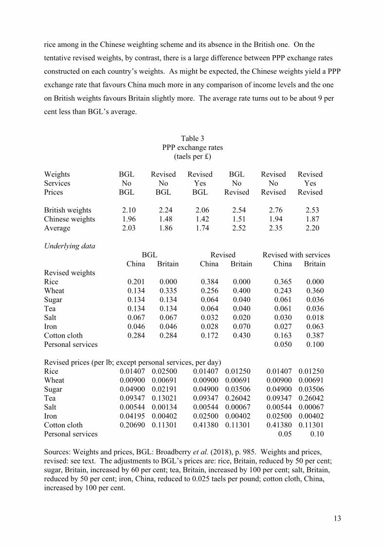
13

rice among in the Chinese weighting scheme and its absence in the British one. On the

tentative revised weights, by contrast, there is a large difference between PPP exchange rates

constructed on each country’s weights. As might be expected, the Chinese weights yield a PPP

exchange rate that favours China much more in any comparison of income levels and the one

on British weights favours Britain slightly more. The average rate turns out to be about 9 per

cent less than BGL’s average.

Table 3 PPP exchange rates

(taels per £) Weights BGL Revised Revised BGL Revised Revised Services No No Yes No No Yes Prices BGL BGL BGL Revised Revised Revised British weights 2.10 2.24 2.06 2.54 2.76 2.53 Chinese weights 1.96 1.48 1.42 1.51 1.94 1.87 Average 2.03 1.86 1.74 2.52 2.35 2.20 Underlying data BGL Revised Revised with services China Britain China Britain China Britain Revised weights Rice 0.201 0.000 0.384 0.000 0.365 0.000 Wheat 0.134 0.335 0.256 0.400 0.243 0.360 Sugar 0.134 0.134 0.064 0.040 0.061 0.036 Tea 0.134 0.134 0.064 0.040 0.061 0.036 Salt 0.067 0.067 0.032 0.020 0.030 0.018 Iron 0.046 0.046 0.028 0.070 0.027 0.063 Cotton cloth 0.284 0.284 0.172 0.430 0.163 0.387 Personal services 0.050 0.100 Revised prices (per lb; except personal services, per day) Rice 0.01407 0.02500 0.01407 0.01250 0.01407 0.01250 Wheat 0.00900 0.00691 0.00900 0.00691 0.00900 0.00691 Sugar 0.04900 0.02191 0.04900 0.03506 0.04900 0.03506 Tea 0.09347 0.13021 0.09347 0.26042 0.09347 0.26042 Salt 0.00544 0.00134 0.00544 0.00067 0.00544 0.00067 Iron 0.04195 0.00402 0.02500 0.00402 0.02500 0.00402 Cotton cloth 0.20690 0.11301 0.41380 0.11301 0.41380 0.11301 Personal services 0.05 0.10 Sources: Weights and prices, BGL: Broadberry et al. (2018), p. 985. Weights and prices, revised: see text. The adjustments to BGL’s prices are: rice, Britain, reduced by 50 per cent; sugar, Britain, increased by 60 per cent; tea, Britain, increased by 100 per cent; salt, Britain, reduced by 50 per cent; iron, China, reduced to 0.025 taels per pound; cotton cloth, China, increased by 100 per cent.

14

The effects of taking into account differences in the costs of personal services can also be

explored. Such services are mostly labour, so their prices might be represented by the wages of

unskilled labourers. As noted above, much of service sector output was composed of inputs to

the production of agricultural and industrial goods, so the weights for personal services would

be a good deal less than the share of services in output. Since the British service sector was a

good deal larger than China’s, tentative weights of 10 per cent for Britain and 5 per cent for

China will be tried and the weights on the other goods reapportioned accordingly. The result

is, as might expected, a further, yet relatively modest fall in the PPP exchange rates, more so

on British weights than on Chinese weights.

So far, the revisions of the weighting would suggest that BGL’s PPP exchange rates will tend

to understate the level of income in China relative to Britain, but there are problems with some

of the prices they have used and some tentative adjustments are proposed here. Among the

British prices, those for tea and sugar exclude duty, yet it is final consumption prices that

should figure in the calculation of PPP exchange rates. Including tariff would roughly double

the tea price and increase the sugar price by about 60 per cent. The exclusion of the duties

overstates purchasing power in Britain, hence would further lower the PPP exchange rate. On

the other hand, the British price for salt, from Greenwich hospital, seems somewhat high, as it

was more than four times the average declared value of salt exports (UK PP 1903 LXVIII

(321), p. 190). This average value was roughly equal to the Liverpool price, the main port

from which salt was exported, and even fishermen on the west coast of Ireland were able to

purchase salt at only 2-3 times the Liverpool price (UK PP 1837 XII (77), pp. 123, 141, 193).

Reducing BGL’s salt price by half would bring it more in line with this experience.

Iron has a relatively small weight in the PPP calculations, but its tael per £ ratio is very high, at

10.44. BGL’s Chinese price is for wrought iron, whereas their British price is for bar iron.

The value of imports of British bar iron at Canton in 1844-5 averaged 0.0259 taels per lb, less

than BGL’s 0.4195 and the average price of Chinese bar iron imports earlier in the 1840s was

reckoned at 0.0207 taels per lb (UK PP 1844 LI (570), p. 6; 1846 XLVI (647), p. 24; 1847 XL

(1286), p. 67). A report by a Swedish commercial agent in 1847 indicated that Chinese

producers could supply first quality bar iron at Canton for a price equivalent to the import price

(Wagner 2008, p. 75). These figures suggest that the Chinese price for bar iron be reduced

from to 0.04195 about 0.025 taels per lb.

15

But the prices that really matter, especially on the revised weighting, are those for grains and

cotton cloth. BGL have only one British rice price, for a purchase by the Lord Steward’s

Department in 1830, yet the prices of rice imported from Bengal were regularly quoted in

London and Liverpool price currents c.1840. The average price for 1838-42, duty included,

was £0.0067 per lb, which would produce a taels per £ ratio of 2.11, much higher than BGL’s

0.56 (Public Ledger (London) and Liverpool Mercury, 1838-42). Allowing for the costs of

distribution within Britain would bring down this ratio, say to about half of BGL’s price. As

for cotton cloth prices, testimony about exports of cotton cloth before the Select Committee on

Commercial Relations with China in 1847 included direct comparisons of the costs in pounds

sterling of shipments made from England with the proceeds in Mexican dollars of sales in

China in 1844 and 1845 (UK PP 1847 V, pp. 148-150).4 One set of comparisons, for 72 reed

gray shirting sent to Shanghai, produces an average tael per £ ratio of 4.78; the other, for

general cargoes of cloth sent to China, 3.44. Both of these values are a good deal higher than

BGL’s 1.83. Since cotton cloth was a very heterogeneous good, these comparisons have the

great advantage of comparing the same quality of cloth. They suggest that the Chinese price of

cotton cloth be roughly doubled to achieve a tael per £ ratio of somewhat less than four.

The effects of revising the British and Chinese prices along the lines suggested in the preceding

paragraphs are also shown in Table 3. The price revisions work in the opposite direction to

the revision of the weights; they increase purchasing the power parity exchange rate, making it

less favourable to China. On BGL’s weighting scheme the PPP exchange rises by 24 per cent;

on the revised weighting scheme by 26 per cent. Overall the price revisions dominate the

weighting revisions, so that the PPP exchange rate with both revised prices and revised weights

is 17 per higher than BGL’s. Taking account of personal services reduces the difference to 8

per cent. These calculations suggest that BGL may be overstating somewhat the level of

China’s output per capita relative to that of Britain at their 1840 benchmark

In general, it must be admitted that the evidence available to calculate these purchasing power

parity exchange rates is quite scant. The range of prices is very limited, only seven

commodities. The prices are sometimes wholesale, sometimes closer to retail. Some prices are

those at the ports, either for export or import; others may have a broader geographical

coverage. The prices used by BGL other than the ones discussed here may also need revision

and the revised prices proposed here may be subject to criticism. On the whole, the main

4 The Mexican dollar, which circulated as coin, was worth about 1.38 taels, which was more a unit of account.

16

conclusion to be drawn is that such calculations of purchasing power exchange rates must have

a very wide margin of error.

A more general concern is how well a purchasing power exchange rate in 1840 can capture the

differences in price levels between China and Britain in earlier periods. For example, it is

highly likely that before the late eighteenth century the price of cotton cloth in China relative to

that in Britain was much lower. At that time raw cotton was much cheaper in Asia than in

Europe and the mechanization of spinning and weaving was still in the future. Between the

sixteenth and nineteenth centuries Britain went being a salt importer to being the world’s

largest exporter, which might suggest that the price of salt in Britain relative to that in China

had fallen (Adshead 1992, pp. 104). The potential biases induced by comparing GDP in

Britain and China in, say, 1400 using a PPP exchange rate for 1840 are comparable to those

highlighted by Prados de la Escosura (2000) for nineteenth-century comparisons based on 1990

PPP exchange rates.

The Early Qing Peak

The peak in GDP per capita in 1700 and the very rapid decline thereafter, which are central to

BGL’s dating of the Great Divergence from the early eighteenth century, are almost entirely

due to the series for population used by BGL. As shown in Solar’s comment, the series for

grain output accounts for over 70 per cent of the GDP estimates. During the late seventeenth

and early eighteenth centuries BGL actually have information on the amount of cultivated land

and on crop yields for only three years. Their decadal estimates for grain output are

interpolations among these years, at 0.63 per cent per annum between 1685 and 1724 and 0.41

per cent between 1724 and 1766; between 1690 and 1750 the annual growth would be 0.53 per

cent. As for population, their figures show a decline by 0.42 per cent per annum between 1690

and 1700, then growth at 1.27 per cent per annum to 1750; from 1690 to 1750 the annual

growth rate would be 0.99 per cent. Other estimates of population growth from 1690 to 1750

are lower, with those by Xu et al coming in at 0.83 per cent per annum, by Shi at 0.81 per cent

and by Cao at 0.41 per cent. These alternative views about population growth all make the fall

in agricultural output per capita from the 1690 to the 1750 less steep, and Cao’s estimates turn

it into a modest increase.

17

The sharp peak in 1700 results both from the very rapid growth assumed in the decades

thereafter and from the fall in population between 1690 and 1700 in their original series.

BGL provide no justification for this fall during the 1690s. The literature may contain major

wars, famines or epidemics that could potentially explain a fall of this magnitude over a

decade, but if wars or famines, then agricultural output would probably also have fallen. But,

given that BGL have data on neither the cultivated area nor crop yields in the 1690s, their

estimates of grain output could not have picked this up.

In their eagerness to show “the small differences between our estimates and those of other

scholars” (p. 966), BGL put forward their Figure 5, which shows their estimates and those of

Shi over the period from 1660 to 1820. Note that they exclude the estimates by Xu et al and by

Cao, which appeared on Solar’s Table 2 and Figure 4, and yet they accuse Solar of “selective

use of the data” (p. 966). What is more damning is that they also leave out the population

series that they used to calculate GDP and GDP per capita in both their article and their

restatement. The population figures in the replication file for the article are completely

different from those in the replication file for the restatement that relate to Figure 5. Note, too,

that the replication file for the restatement contains the figures from Xu et al, but these figures

somehow did not find their way onto Figure 5. Note further that the population of China in

1700 is shown as about 160 million on their Figure 5, even though two pages earlier it is given

in the text as 138 million (p. 965). (This last inconsistency was pointed out to Stephen

Broadberry on 29 March 2021 and to the editors of the Journal of Economic History on 3 June

2021, but was never corrected.)

The population figures missing from BGL’s Figure 5 are shown in Figure 3. BGL’s original

figures show not only a fall from 1690 to 1700 followed by very fast growth, as noted above;

they also show a very sharp deceleration in population growth from 1750, with the annual rate

of growth falling from 1.27 per cent to 0.55 per cent. The figures shown in the restatement’s

Figure 5 show a much gentler deceleration from 1.06 per cent per annum up to 1724 to 0.79

per cent thereafter. By contrast, Xu et al assume that growth remained constant at 0.83 per

cent from 1690 to 1766 and Cao’s point estimates imply growth of 0.41 per cent between 1680

and 1776. In further contrast, Shi sees an acceleration in 1724, from 0.59 per cent to 1.10 per

cent. Both Cao’s and Shi’s population growth rates to 1724 would imply that grain output per

capita was not falling from the late 1680s to the mid-1720s, essentially eliminating the rise and

fall in estimated GDP per capita around the turn of the eighteenth century.

18

Figure 3 Various Series for the Population of China, 1690-1766

(log scale)

Sources: Broadberry, Guan and Li (2018, 2021), Xu et al (2017), Shi (2020), Cao (2022). Note that the level of China’s population in 1680 in Cao’s new estimates (185 million) is higher than that (160 million) shown in Table 2 in Solar (2021).

As Solar noted in his comment, all of these estimates result from projections backward from

somewhat more reliable population figures from the later eighteenth century. The range of

trajectories and levels shown in Figure 3 are indicative of considerable uncertainty about early

Qing population. BGL’s population series comes from Maddison (2007), who relied on Liu

and Hwang (1977), who, in turn, state that they based their work on Perkins’ (1969)

benchmarks. Perkins himself promised no particular accuracy for his population figures for

the seventeenth and eighteenth centuries:

“There is no way yet discovered for reliably estimating population under the Ch’ing

in the late seventeenth century, although I shall make a few remarks on this subject

below.” (p. 202)

“If one accepts a total of 400 million for the early nineteenth century, and further

accepts the evidence of prosperity during the latter half of the eighteenth century, it

4.4

4.6

4.8

5

5.2

5.4

5.6

5.8

1690 1700 1710 1720 1730 1740 1750 1760

BGL 2018

BGL 2021

Xu et al

Shi

Cao

19

is reasonable to assume that population was about 200 to 250 million around 1750.”

(p. 208)

“Depending on what assumptions one makes about population growth from 1650 to

1750, one can get a figure for the 1650’s ranging from 100 to 200 million. If one

believes, as I do that population grew between 1650 and 1750, then a range of from

100 to 150 million for 1650 would appear to cover the most probable situation.” (p.

209)

Although Perkins thus only put forward ranges at mid-centuries, Liu and Hwang give single

figures by decade. They put China’s population in 1650 at 123 million, close to the mid-point

of Perkins’ range, but their figure for 1750 is 260 million, higher than the upper end of Perkins’

range, for which they provide no justification (pp. 80-81). Liu and Hwang then used the raw,

greatly understated official counts to estimate the intervening values by trend-corrected

interpolation. It is, in part, their assumption that undercounting was reduced continuously at a

constant rate over the century which creates the trough in 1700 that is partly responsible for the

sharp peak in GDP per capita. But, actually, rapid population growth between 1700 and 1730

does not appear in Liu and Hwang’s series. Maddison (2007, pp. 165, 168) thought the growth

in population between 1730 and 1750 shown by their figures was implausible and assumed that

China’s population grew at a constant rate between Liu and Hwang’s estimates for 1700 and

1750. He provided no justification for why he chose these years, as against any others, as

reliable benchmarks between which to interpolate.

Liu and Hwang, both based in Taiwan, do not seem to have done any other work on the

historical demography of the mainland. Their estimates, apparently produced as a one-off for a

conference, as well as Maddison’s revision of them, illustrate how numbers, once created, can

become entrenched as unchallenged facts.5 Maddison (2007, p. 165) himself did not

understand how Liu and Hwang filled the gaps between Perkins’ ranges. Strangely, neither

Maddison nor BGL have fully engaged with the much more extensive work of Cao (2000,

2001). BGL do cite his books on Ming and Qing population history, but prefer in their

restatement to compare their population figures only to those of Shi (2020), who is primarily

an agricultural historian. Shi’s critical review of Cao’s estimates is limited to one sentence in a

footnote: “I think that his estimates are too high to believe” (2020, p. 179).

5 On the more general weaknesses of figures hazarded for pre-industrial populations by McEvedy and Jones and Maddison, as well as on their misuse by economists and economic historians, see Guinnane (2021).

20

The uncertainty concerning early Qing population does not necessarily have implications for

population during the Ming since most estimates for that period are projections forward from

the late fourteenth century. The Liu and Hwang/Maddison/BGL estimates for this period may

well have their own problems. New estimates by Cao (2022) show generally lower levels of

population during the Northern Song and higher levels during the Ming.

The Greats—Divergence, Convergence and Crossing

What does all this mean for comparing China and Europe over the long term? Solar is

generally skeptical about the estimates because they are based, essentially, only on series for

grain output and population. Given that skepticism and the problems with the revisions to the

government sector, the 1840 benchmark and the population figures for the late seventeenth and

early eighteenth century, what might still be gleaned from BGL’s work? One guess, and it is a

guess, would have the following features: 1) a 1840 benchmark of $535 based either on Xu et

al and Ma and de Jong or on the revision of the PPP exchange rates; 2) Xu et al’s benchmark

estimates (with linear interpolation of intervening years) of GDP per capita back to 1661,

which are based on a broader sectoral coverage than BGL’s and make use of a more realistic

population series; and 3) coverage of the Ming and Northern Song periods using the GDP per

capita series in Solar that is based on the assumption of a constant government share, that is,

dispensing both with BGL’s revised government series for the Northern Song and Ming and

with their revision of the series for cultivated land upward during the Ming. Two versions of

these guesstimates are shown in Figure 4: one uses BGL’s population figures for the Northern

Song and the Ming and Xu et al’s for the Qing; the other uses Cao’s (2022) recent numbers.

The different population series clearly lead to different stories about China’s development over

the centuries. The series based on BGL’s and Xu et al’s population numbers still shows a peak

in the mid-seventeenth century (instead of c.1700) comparable to that in the Northern Song.

Incomes decline rapidly from then until the mid-nineteenth century. Cao’s figures, by contrast,

show incomes to be comparable in the Ming and Qing, with decline setting in only from the

mid-eighteenth century. In the mid-seventeenth century there is the hint of a trough in GDP

per capita instead of a peak. Cao’s figures also prolong and augment the peak in the Northern

21

Song, and they leave a greater gap between incomes in the late Northern Song and the early

Ming.

Figure 4 Guesstimates of GDP per capita, 980-1840: Alternative population series

(1990 $)

Sources: see text. What implications do these figures have for the Great Divergence debate? In their

comparisons with Western Europe, BGL, following Pomeranz (2000) and others who argue

that advanced regions in Europe should be compared to advanced regions in China, focus on

the Yangzi delta region and create what they term an upper bound estimate for GDP per capita

in this region (in the restatement the notion of an upper bound disappears in favour of

describing the series as “China leader”). This involves a constant upward adjustment of 75 per

cent to their estimates of China’s GDP per capita from 980 to 1840. This adjustment factor is

based on Li and van Zanden’s (2012) estimate of GDP per capita in the 1820s for the Hau-Lou

area, now part of metropolitan Shanghai, hence at the heart of the delta. As BGL have pointed

out, Solar incorrectly interpreted their adjustment factor and should have applied a higher

factor, more like 87 per cent, to his revised series. More problematic is the assumption that at

all times during more than eight centuries GDP per capita in the leading region in China was

always 75 (or 87) per cent higher than for China as a whole. The Yangzi delta’s advantage

over the rest of China may have been at its peak in the 1820s, the time at which Li and van

Zanden make their comparison. Ma (2008) estimated that incomes in the delta in the 1930s

0

200

400

600

800

1000

1200

980 1030 1080 1130 1180 1230 1280 1330 1380 1430 1480 1530 1580 1630 1680 1730 1780 1830

BGL/Xu et al

Cao

22

were only 55 per cent higher than the Chinese average and cited evidence that the region’s land

tax revenue per capita in the mid-eighteenth century was only 44 per cent higher than the

national average. Allen et al (2011) found that wages in the delta in the mid-eighteenth

century were not distinctly higher than elsewhere in China. Ma’s figures refer to a Yangzi

delta region of tens of millions of inhabitants; the Han-Lou district contained only about half a

million. The area was heavily involved in cotton textile production. As such, it had prospered

during the eighteenth and first decades of the nineteenth century, whilst at the same time

population pressure had driven down incomes in agriculture, the dominant sector in the rest of

China. But from the 1820s the domestic market for cotton textiles “practically collapsed” and

British yarn and cloth began to make inroads in Asian markets (Li 2009; Zurndorfer 2009). An

adjustment factor of 75 (or 87) per cent may thus overstate the delta’s relative prosperity in

other periods.

The assumption of a constant adjustment factor has another, perhaps awkward, implication.

Pomeranz (2000, p. 288) notes that “The most advanced prefectures of the Yangzi Delta, which

had roughly 16-21 per cent of China’s population in 1750, were barely 9 per cent of the empire

by 1850, and about 6 per cent by 1950” (the estimates in Xu et al (2018) show somewhat less

of a fall). If, the Yangzi delta’s share in China’s population was falling, the implication of a

constant relationship between income per capita in the Yangzi delta and the average for China

as a whole would thus be that the difference in incomes between the delta and those in the rest

of China had been even wider in earlier centuries than it was in the early nineteenth century.

Whilst BGL focus on comparing leading regions in Europe and China, another way to

investigate the timing of the Great Divergence would be to compare GDP per capita in Western

Europe as a whole to that of China. Although, as for China, one might have qualms about

placing too much faith in the historical series for GDP per capita in European countries, there

are now series for England/later Britain, Holland/later the Netherlands, France, Spain, northern

and central Italy and Germany, countries which made up about 80 per cent of Western

Europe’s population both in 1500 and 1850, the period over which series for all of these

countries exist.6 The main missing country is the Austrian territories, which, in terms of

income per capita, were likely to fall somewhere in the middle, between the leaders

(successively Italy, Netherlands, England) and the laggard (Spain). Figure 5 compares GDP

6 Series also exist for two smaller countries, Sweden (Schoen and Kranz 2012; Edvinsson 2013) and Portugal (Palma and Reis 2018), but do not reach back to 1500.

23

per capita for the parts of Western Europe comprised by six counties mentioned above to that

for China at several benchmark dates.

Figure 5 GDP per capita in “Europe” and China, 1500-1850

(1990 $)

Sources: European GDP per capita: England, Holland, Italy, Spain and Germany: Palma and Reis (2019), p. 500; France: Ridolfi and Nuvolari (2021), supplementary material online, five-year centred averages. European population: 1500-1650: de Vries (1994), p. 13; 1700-1850: Malanima (2010), p. 257. China: see text. The first thing to note is that, from at least 1500, GDP per capita in Western Europe was

always higher than in China. Using Cao’s population figures the European advantage varied

between 73 and 100 per cent before 1800 and it is difficult to see any great divergence during

the sixteenth, seventeenth or eighteenth centuries. There may have been some very modest

widening of the gap during the eighteenth century, but most of the action seems to have taken

place during the early nineteenth century as Europe, led by Britain, surged ahead. The steady

level of GDP per capita during the Ming and Qin shown by this series is consistent with Chen

and Peng’s (2022) conclusions about the trends in rice wages, in the relative prices of silk and

rice and in various forms of consumption.

0

200

400

600

800

1000

1200

1400

1600

1800

1500 1550 1600 1650 1700 1750 1800 1850

Europe

China (BGL/Xu et al)

China (Cao)

24

On BGL’s and Xu et al.’s population figures there does seem to have been significant

divergence from the mid-seventeenth century, as incomes rose in Europe and, more

importantly, fell steadily in China. But it would be awkward to date the Great Divergence

from this time without some understanding of why incomes in China and Europe had

previously converged, especially in the early seventeenth century. This convergence might be

real or an artifact of the estimates or a bit of both. The transition from the Ming to Qing in the

1630s, 1640s and 1650s was marked by famines, wars and a major plague epidemic, with

figures cited for population losses, often covering different periods, on the order of about a

fifth (Parker 2013). The fall in numbers increased the land/labour ratio, which should have

raised incomes in the agricultural sector. But if it led to less intense cultivation, then the

methods used by BGL and Xu et al to estimate agricultural output may have led to its

overstatement. In so far as the rise in China’s income per capita was the real consequence of

the fall in population, then the income per capita should have subsequently fallen as population

recovered. This would be an argument for treating divergence as beginning from the mid-

eighteenth rather than the mid-seventeenth century. Yet it is indeed strange that in Europe,

which also suffered from plague and war in the mid-seventeenth century, incomes failed to

rise. On the estimates for GDP per capita based on BGL’s and Xu et al’s population figures,

the seventeenth century crisis seems to have played out very differently in China than it did in

Europe.

Were incomes in Europe always significantly higher than they were in China? BGL take

umbrage at Solar’s suggestion, described only as a hypothesis, that their figures would imply a

Great Crossing sometime in the Middle Ages (p. 966). They seem to suggest that this could

only be established with GDP data for the European leader before 1300 and for China in the

gap between the Northern Song and the Ming, even though in their original article, before the

revision of Ming GDP per capita downward, they conclude that “Although China had the

highest standard of living in the world during the Northern Song dynasty, Italy had already

forged ahead by 1300” (p. 993). Only four countries—France, England, Italy and Spain—have

historical GDP accounts going back to 1300. Taken together, they imply that GDP per capita

in “Europe” was 1007 1990$ at that time. BGL’s original and revised estimates for the

Northern Song at its peak in 1020 are 997 1990$ and 1016 1990$, which imply that for there to

have been no crossing, income per capita in Europe would have had to be constant or have

declined during the eleventh, twelfth and thirteenth centuries. On the guesstimates using Cao’s

population figures, the Northern Song peak was 972 1990$. This leaves a little room for

25

growth to have occurred in Europe during these centuries, though the Chinese GDP per capita

in that year (1080) was already higher than GDP per capita in France, England and Spain in

1300 (the leading economy, Italy, pulled up the average for that year). In support of the

hypothesis of a crossing, Solar’s comment cited work on urbanization and manuscript

production that suggests contrasting trends in Italy and China during these centuries.

Subjective margins of error

BGL cite the example of Perkins who assigned margins of error to his estimates for population.

They are inspired by his assessment that his mid-nineteenth century estimates for Qing

population within a margin of 6 per cent to accord all Qing population figures back to 1690

their A grade (firm figures: ±less than 6 per cent; average margin of error ±2.5 per cent). In

fact, Perkins reckoned only that there was “perhaps an 80 per cent chance” that the true value

lay in this range (p. 216). Yet, as shown above, Perkins though that China’s population in

1650 was between 100 and 150 million and in 1750 between 200 and 250 million, indicating

error margins of ±20 per cent and ±11 per cent, qualifying for grades C and B, respectively.

Based on the range of estimates shown in Figure 3 for the years between 1690 and 1720, the

average margin of error would be about ±9 per cent, again grade B.

BGL congratulate themselves on the use of margins of error, yet they are very selective in the

way that they report results that do not fall within them. Although they accorded their

estimates for government during the Ming a B grade (5 to 15 per cent), the average difference

between the old and new estimates is 57 per cent. Instead, they focus on GDP, stating that

“Although the difference averages 13.8 per cent for the Ming dynasty as a whole, this falls to

10.5 per cent during the decades after 1490. Both figures are within the 5 to 15 per cent

subjective error margins offered for Ming GDP…” (p. 963). Of course, an obvious

implication of these numbers is that before 1490 the difference was greater; it was 17.7 per

cent or 21.8 per cent, depending on whether one uses the old or new estimate as the

denominator. But remember that BGL have taken their reply as an occasion also to raise Ming

cultivated land by 9.3 per cent, which has the effect of raising GDP per capita by 6.7 per cent.

Without this change, the above sentences would read: “Although the difference averages 19.2

per cent for the Ming dynasty as a whole, this falls to 16.3 per cent during the decades after

1490. Both figures are outside the 5 to 15 per cent subjective error margins offered for Ming

26

GDP…” For the early Ming the differences average 22.9 or 30.0 per cent, again depending on

the choice of denominator.

But what do these margins of error mean for the historian, who is generally concerned not so

much with whether any given figure for population or GDP per capita is correct, but with the

comparison of two or more figures, over time or across space. Most of BGL’s series are

designated as grade B (±5 to 15 per cent; average margin of error, ±10). What does this

average margin of error imply for what a researcher might find concerning comparisons over

time? Suppose that there is, in fact, no change between the two dates and that the errors at the

two dates are uncorrelated. In this case the researcher will have about a four per cent chance of

finding an increase or decrease of at least 15 per cent and a 17 per cent chance of finding an

increase or decrease of at least 10 per cent, not insignificant amounts given the scale of

changes in per capita incomes during the pre-industrial period. Of course, if the errors were

correlated, then the risks of misjudging a change would be much reduced. Hence the

researcher ought to be as concerned with whether or not the errors might be correlated as with

the margins of error.

Replication

When scholars more familiar with Chinese sources set about assessing BGL’s estimates, they

may find the task somewhat difficult. The replication files for the article and the restatement

are often quite summary and, even by reference to BGL’s 2017 working paper (no online

appendix was found and it does not accompany the replication file), it is not always easy to

work out what exactly they have done. They do not have data for every decade and many of

the extrapolations and interpolations are unexplained. In some cases, the data presented would

not be sufficient to assess the reliability of the estimates. Take, for example, the government

sector, which was estimated initially, according to the working paper, by multiplying the

numbers of civil servants and soldiers by their salaries. The replication file for the article

contains information on neither numbers nor salaries, only the resulting figures for total

nominal expenditure. In the restatement, government spending in the Northern Song is based

on the numbers of solders and civil servants, data on which are given in the replication file at

decadal frequency. Yet the series grows at a constant rate over the period, suggesting that it

was created by interpolation or extrapolation between two unidentified and undocumented data

points.

27

Conclusions

BGL’s standard response to many criticisms is that they don’t make any difference to the

estimates or to their dating of the Great Divergence. This is too facile since, as both Solar’s

Table 3 and BGL’s own sensitivity analysis in the article showed, unless a series, like the

original one for government, is extremely out of whack, nothing would indeed matter except

for errors in the series for grain output, which accounts for over 70 per cent of the GDP

estimates, or in that for population, which accounts for another 20 per cent, as well as being the

divisor for calculating per capita GDP. On these grounds, BGL might well have used just

these two series, making the basis for their estimates much clearer to the reader. But it would

also have put greater onus on them to justify the grain output and population series as

consistent, accurate and appropriate measures of what was happening in the Chinese economy

over almost a millennium. As shown above, the population figures are subject to considerable

uncertainty. As for grain output, Deng and O’Brien (2016) have cast doubt on whether the

land tax returns can be turned into good estimates of the area of cultivated land. Recent work

questions whether the available evidence on rice and wheat yields may be subject to selection

bias (Chen and Peng 2022; Ma and Peng 2022). The verdict of other scholars of Northern

Song, Ming and Qing China on the evidence used by BGL can only be awaited.

Since the sources for medieval and early modern Chinese history are generally regarded as

notoriously difficult to interpret, such testing is probably in order, yet it seems to have been

quite limited. To judge from the article’s acknowledgements, the original paper was presented

only at seminars and conferences in Europe and North America and commented on in detail

only by scholars located in those regions, only one of whom is a China specialist. (Nor is

Solar expert on Chinese economic history, for that matter.) Given the huge problem with the

government sector in the original paper and the treatment of population figures in both the

original paper and in the restatement, it does seem that the article’s other readers, the referees

at the Journal of Economic History, as gatekeepers on research that is sure to be widely cited,

did not engage fully with the underlying data and estimation procedures.

Nor do the authors have a track record of publications on medieval and early modern China,

the period covered by the estimates. Broadberry has worked primarily on Britain, though in

recent years has been active in historical national accounting for a number of places around the

world. Li is an economist who has published widely on foreign direct investment, state-owned

28

enterprises and other topics of current policy in China, yet he has published no work in Chinese

economic history unrelated to the GDP estimates. Guan is an economic historian who has

published mainly on various aspects of Chinese experience during the late nineteenth and early

twentieth centuries, although he has also worked on monetary history in the second century BC

and on the rise of the civil service examinations during the seventh and eighth centuries AD.

The only acknowledged research assistance was provided by Pei Gao, an economic historian

who has published primarily on human capital formation during the late nineteenth and early

twentieth centuries.

Venturing into more than eight centuries of Chinese economic history is an audacious

endeavour and, as such, requires careful scholarship. Both the article and the restatement are

wanting in this respect. BGL’s initial government sector estimates should never have survived

the smell test. Their implementation of weighting for the 1840 benchmark has been

persistently sloppy. Their treatment of the various population estimates has been cavalier at

best. Solar’s comment and this working paper have revealed inconsistencies, errors and

lacunae (more are laid out in the Appendix). BGL have also been ungracious toward other

scholars, making only little or selective use of the work of Cao, Liu, Xu et al, Ma and de Jong,

and Xu et al (2018).7 Admittedly, some of this work was only published just before or after

BGL’s article, but it had been circulating in working papers well before the article was

published and was published well before the restatement. In addition, BGL have shown a

reluctance to engage with non-quantitative evidence on the state of the Chinese economy. All

of this should make for considerable skepticism about whether they got either the trends or the

fluctuations in China’s GDP per capita right.

7 The last-mentioned’s results on urbanization are more soundly based than those used by BGL.

29

References

Adshead, S.A.M. Salt and Civilization. New York: St Martin’s Press, 1992.

Allen, Robert C., Jean-Pascal Bassino, Debin Ma, Christine Moll-Murata, et al. “Wages, Prices, and Living Standards in China, 1738–1925: In Comparison with Europe, Japan and India.” Economic History Review 64, no. 1 (2011): S8–S38.

Broadberry, Stephen, Bruce Campbell, Alexander Klein, Mark Overton, and Bas van Leeuwen. British Economic Growth, 1270–1870. Cambridge: Cambridge University Press, 2015.

Broadberry, Stephen, Johann Custodis, and Bishnupriya Gupta. “India and the Great Divergence: An Anglo-Indian Comparison of GDP per Capita, 1600–1871.” Explorations in Economic History 55 (2015): 58–75.

Broadberry, Stephen, Hanhui Guan, and David Daokui Li. “China, Europe, and the Great Divergence: A Study in Historical National Accounting, 980–1850.” University of Oxford Discussion Papers in Economic and Social History, no. 155, April 2017.

Broadberry, Stephen, Hanhui Guan, and David Daokui Li. “China, Europe, and the Great Divergence: A Study in Historical National Accounting, 980–1850.” Journal of Economic History 78, no. 4 (2018): 955–1000.

Broadberry, Stephen, Hanhui Guan, and David Daokui Li. “China, Europe, and the Great Divergence: A Study in Historical National Accounting, 980–1850 [Data set].” Ann Arbor, MI: Inter-university Consortium of Political and Social Research, 2018. Available at http://doi.org/10.3886/E105383V1.

Broadberry, Stephen, Hanhui Guan, and David Daokui Li. “China, Europe, and the Great Divergence: A Restatement.” Journal of Economic History 81, no. 3 (2021): 958-974.

Broadberry, Stephen, Hanhui Guan, and David Daokui Li. “China, Europe, and the Great Divergence: A Restatement.” Ann Arbor, MI: Inter-university Consortium for Political and Social Research [distributor], 2021- 05-12. https://doi.org/10.3886/E132382V2.

Broadberry, Stephen, and Bishnupriya Gupta. “The Early Modern Great Divergence: Wages, Prices and Economic Development in Europe and Asia, 1500–1800.” Economic History Review 59, no. 1 (2006): 2–31.

Cao, Shuji. Zhongguo renkoushi, Vol. 4: Ming shiqi (Chinese Population History, Vol. 4: Ming dynasty). Shanghai: Fudan University Press, 2000.

———. Zhongguo renkoushi, Vol. 5: Qing shiqi (Chinese Population History, Vol. 5: Qing dynasty). Shanghai: Fudan University Press, 2001.

Cao, Shuji. “Population Change.” In The Cambridge Economic History of China, edited by Debin Ma and Richard van Glahn, vol. 1. Cambridge: Cambridge University Press, 2022.

Chang, Chung-li. The Income of the Chinese Gentry. Seattle: University of Washington Press, 1962.

30

Chen, Zhiwu and Kaixiang Peng. “Consumption and Living Standards since the Song Dynasty.” In The Cambridge Economic History of China, edited by Debin Ma and Richard van Glahn, vol. 1. Cambridge: Cambridge University Press, 2022.

de Vries, Jan. “Population.” In Handbook of European History, 1400-1600, edited by Thomas A. Brady, Heiko A. Oberman and James D. Tracy, pp. 1-50. Leiden: Brill, 1994.

Deng, Kent, and Patrick K. O’Brien. “China’s GDP Per Capita from the Han to Modern Times.” World Economics 17 (2016): 79–123.

Deng, Kent, and Lucy Zheng. “Economic Restructuring and Demographic Growth: Demystifying Growth and Development in Northern Song China, 960-1127.” Economic History Review 68, no. 4 (2015): 1107-1131.

Edvinsson, Rodney B. “Swedish GDP 1620-1800: Stagnation or Growth?” Cliometrica 7, no. 1 (2013): 37-60.

Guinnane, Timothy W. “We Do Not Know the Population of Every Country in the World for the Past Two Thousand Years.” Cesifo Working Paper 9242 2021, August 2021.

Hao, Yu, and Kevin Zhengcheng Liu. “Taxation, Fiscal Capacity, and Credible Commitment in Eighteenth-Century China: the Effects of the Formalization and Centralization of Informal Surtaxes.” Economic History Review 73, no. 4 (2020): 914-939.

Li, Bozhong. Agricultural development in Jiangnan, 1620–1850. Basingstoke: Macmillan, 1998.

Li, Bozhong. “Involution and Chinese Cotton Textile Production: Sonjiang in the Late Eighteenth and Early Nineteenth Centuries.” In The Spinning World: A Global History of Cotton Textiles, 1200-1850, edited by Giorgio Riello and Prasannan Parthasarathi, pp. 388-395. Oxford: Oxford University Press, 2009.

Li, Bozhong and Jan Luiten van Zanden. “Before the Great Divergence? Comparing the Yangzi Delta and the Netherlands at the Beginning of the Nineteenth Century.” Journal of Economic History 72, no. 4 (2012): 956-989.

Li, Fuming. Zhidu lunli yu jingji fazhan: Mingqing Shanghai diqu shehui jingji yanjiu: 1500–1840 (Institutions, Moral Principles and Economic Growth: Social and Economic Research in Shanghai, 1500–1840). Beijing: Wenshi Press, 2005.

Liu, Paul K.C. and Kuo-shu Hwang. “Population Change and Economic Development in Mainland China since 1400.” In Modern Chinese Economic History, edited by Chi-ming Hou and Tzong-shian Yu, pp. 61-90. Taipei: Institute of Economics, Academia Sinica, 1977.

Liu, Ti. “1600—1840 Nian zhongguo guonei shengchan zong zhi de gusuan (An Estimation of China’s GDP from 1600 to 1840).” Economic Research Journal 44, no. 10 (2009): 144–55.

Liu, William Guanglin. The Chinese Market Economy, 1000–1500. Albany, NY: State University of New York Press, 2015.

31

Ma, Debin. “Economic Growth in the Lower Yangzi Region of China in 1911–1937: A Quantitative and Historical Analysis.” Journal of Economic History 68, no. 2 (2008): 355–92.

Ma, Debin. “Rock, Scissors, Paper: the Problem of Incentives and Information in Traditional Chinese State and the Origin of Great Divergence.” London School of Economics Economic History Working Paper 152/11 (July 2011).

Ma, Debin and Kaixiang Peng. “Agriculture.” In The Cambridge Economic History of China, edited by Debin Ma and Richard van Glahn, vol. 2. Cambridge: Cambridge University Press, 2022.

Ma, Ye, and Herman de Jong. “Unfolding the Turbulent Century: A Reconstruction of China’s Historical National Accounts, 1840–1912.” Review of Income and Wealth 65, no. 1 (2019): 75–98.

Maddison, Angus. Chinese Economic Performance in the Long Run. Paris: OECD, Development Centre Studies, 1998.

Maddison, Angus. Chinese Economic Performance in the Long Run, Second Edition, Revised and Updated, 960-2030 AD. Paris: OECD, Development Centre Studies, 2007.

Malanima, Paolo. “Urbanization.” In The Cambridge Economic History of Modern Europe, Volume 1, 1700-1870, edited by Stephen Broadberry and Kevin H. O’Rourke, pp. 235-263. Cambridge: Cambridge University Press, 2010.

Palma, Nuno, and Jaime Reis. “From Convergence to Divergence: Portuguese Economic Growth, 1527-1850.” Journal of Economic History 79, no. 2 (2019): 477-506.

Parker, Geoffrey. Global Crisis: War, Climate Change & Catastrophe in the Seventeenth Century. New Haven: Yale University Press, 2013.

Perkins, Dwight H. Agricultural Development in China 1368-1968. Chicago: Aldine Publishing Company, 1969.

Pomeranz, Kenneth. The Great Divergence: China, Europe, and the Making of the Modern World Economy. Princeton: Princeton University Press, 2000.

Prados de la Escosura, Leandro. “International Comparisons of Real Product, 1820-1990: An Alternative Dataset.” Explorations in Economic History 37, no. 1 (2000): 1-41.

Ridolfi, Leonardo, and Alessandro Nuvolari. “L’histoire immobile? A reappraisal of French economic growth using the demand-side approach, 1280-1850.” European Review of Economic History 25, no. (2021): 405-428.

Robinson, David M. “Military Labor in China, c. 1500.” In Fighting for a Living: A Comparative History of Military Labour, 1500–2000, edited by Erik-Jan Zürcher, pp. 43–80. Amsterdam: Amsterdam University Press, 2013.

Rozman, Gilbert. Urban Networks in Ch’ing China and Tokugawa Japan. Princeton: Princeton University Press, 1973.

32

Schön, Lennart, and Olle Krantz. “The Swedish Economy in the Early Modern Period: Constructing Historical National Accounts.” European Review of Economic History 16, no. 4 (2012): 529-549.

Shi, Zhihong. Agricultural Development in Qing China: A Quantitative Study, 1661– 1911. Leiden: Brill, 2020.

Solar, Peter. “China’s GDP: Some Corrections and the Way Forward.” Journal of Economic History 81, no. 3 (2021): 943-957.

United Kingdom, Parliamentary Papers, 1837 XXII (77), Commission of Inquiry on the State of Irish Fisheries, First Report.

United Kingdom, Parliamentary Papers, 1844 LI (570), Statement of the Foreign Trade with China.

United Kingdom, Parliamentary Papers, 1846 XLVI (647), Return of Trade at the Ports of Canton, Amoy and Shanghai, 1844.

United Kingdom, Parliamentary Papers, 1847 V (654), Select Committee on Commercial Relations with China.

United Kingdom, Parliamentary Papers, 1847 XL (1286), Returns of Trade at the Various Ports of China, 1845.

United Kingdom, Parliamentary Papers, 1903 LXVIII (321), Report on Wholesale and Retail Prices in the United Kingdom.

Wagner, Donald B. Science & Civilisation in China, Volume V:11. Cambridge: Cambridge University Press, 2008.

Waldron, Arthur N. “The Problem of the Great Wall of China.” Harvard Journal of Asiatic Studies 43, no. 2 (1983): 643-663.

Wong, Hon-chiu. “Government Expenditures in North Sung China (960-1127).” Unpublished Ph.D. thesis, University of Pennsylvania, 1975.

Xu, Xinwu. Jiangnan tubushi (The History of Cotton Production in Jiangnan). Shanghai: Shanghai Social Science Press, 1992.

Xu, Yi, Shi Zhihong, Bas Van Leeuwen, Yuping Ni, Zipeng Zhang, and Ye Ma. “Chinese National Income, ca. 1661–1933.” Munich Personal RePEc Archive Paper No. 70873, Munich, Germany, 2015.

———. “Chinese National Income, ca. 1661–1933.” Australian Economic History Review 57, no. 3 (2017): 368–93.

Xu, Yi, Bas van Leeuwen, and Jan Luiten van Zanden. “Urbanization in China, c.1100– 1900.” Frontiers of Economics in China 13, no. 3 (2018): 322–68.

33

Zhang, Zhongli. “Zhongguo guomin shengchan zongzhi de culue guji in 1800s (An Estimate of China’s National Income in the 1880s).” Nankai Economic Quarterly 1 (1987): 80-106.

Zurndorfer, Harriet T. “The Resistant Fibre: Cotton Textiles in Imperial China.” In The Spinning World: A Global History of Cotton Textiles, 1200-1850, edited by Giorgio Riello and

Prasannan Parthasarathi, pp. 43-62. Oxford: Oxford University Press, 2009

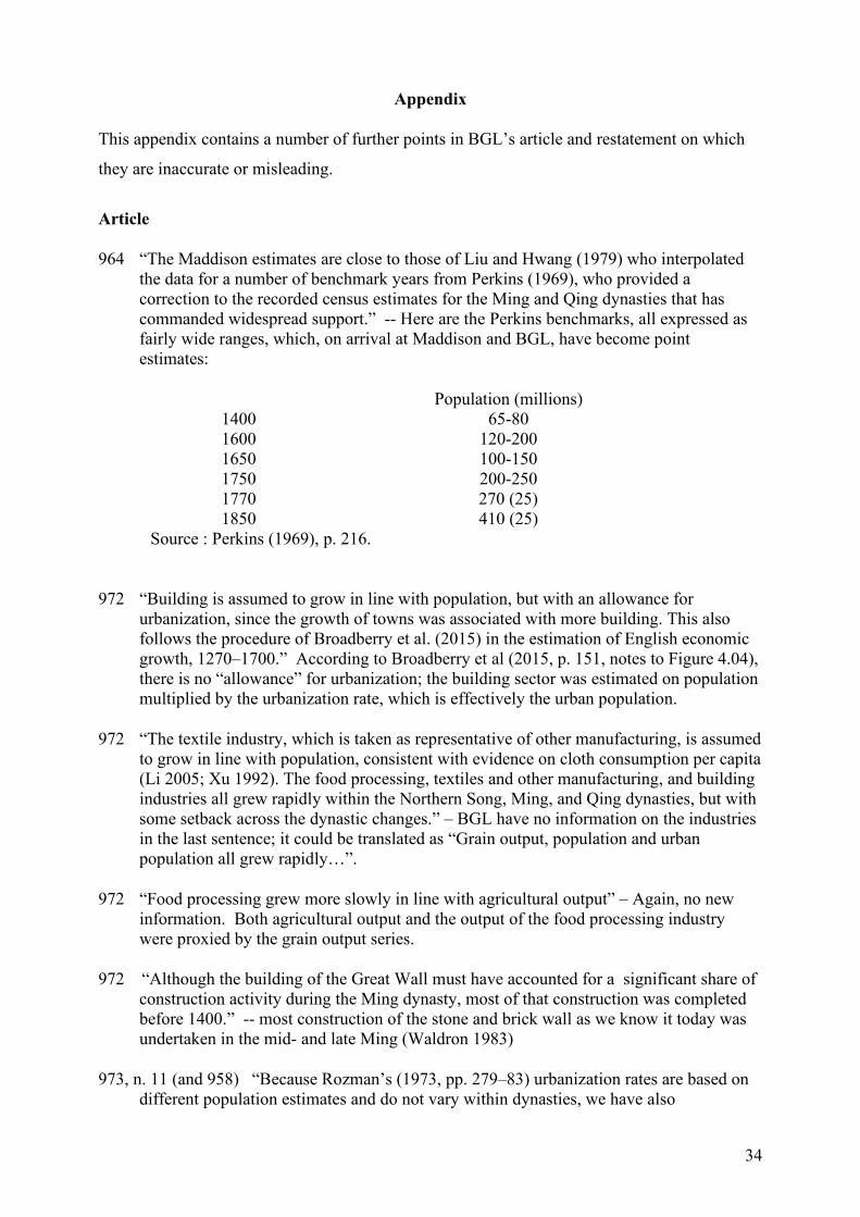
34

Appendix This appendix contains a number of further points in BGL’s article and restatement on which

they are inaccurate or misleading.

Article

964 “The Maddison estimates are close to those of Liu and Hwang (1979) who interpolated the data for a number of benchmark years from Perkins (1969), who provided a correction to the recorded census estimates for the Ming and Qing dynasties that has commanded widespread support.” -- Here are the Perkins benchmarks, all expressed as fairly wide ranges, which, on arrival at Maddison and BGL, have become point estimates:

Population (millions) 1400 65-80 1600 120-200 1650 100-150 1750 200-250 1770 270 (25) 1850 410 (25) Source : Perkins (1969), p. 216.

972 “Building is assumed to grow in line with population, but with an allowance for urbanization, since the growth of towns was associated with more building. This also follows the procedure of Broadberry et al. (2015) in the estimation of English economic growth, 1270–1700.” According to Broadberry et al (2015, p. 151, notes to Figure 4.04), there is no “allowance” for urbanization; the building sector was estimated on population multiplied by the urbanization rate, which is effectively the urban population.

972 “The textile industry, which is taken as representative of other manufacturing, is assumed to grow in line with population, consistent with evidence on cloth consumption per capita (Li 2005; Xu 1992). The food processing, textiles and other manufacturing, and building industries all grew rapidly within the Northern Song, Ming, and Qing dynasties, but with some setback across the dynastic changes.” – BGL have no information on the industries in the last sentence; it could be translated as “Grain output, population and urban population all grew rapidly…”.

972 “Food processing grew more slowly in line with agricultural output” – Again, no new information. Both agricultural output and the output of the food processing industry were proxied by the grain output series.

972 “Although the building of the Great Wall must have accounted for a significant share of construction activity during the Ming dynasty, most of that construction was completed before 1400.” -- most construction of the stone and brick wall as we know it today was undertaken in the mid- and late Ming (Waldron 1983)

973, n. 11 (and 958) “Because Rozman’s (1973, pp. 279–83) urbanization rates are based on different population estimates and do not vary within dynasties, we have also

35

experimented with alternative estimates based on the urban data of Wu (2000) and Cao (2000, 2001). Although this raises the urbanization rate during the early Northern Song period from 6 to 11 percent, the maximum effect of this change is to raise GDP per head above our baseline estimate by 5.7 percent in 980, with most of the effect coming through services rather than industry, since the building industry accounted for just 14.7 percent of industry, with industry accounting for just 8.1 percent of GDP in 1840.” – Are Wu’s and Cao’s estimates better—based on more and better data, more carefully done—than Rozman’s? If so, they should replace Rozman’s; if not, they shouldn’t. The proper criteria should not be whether the effect on GDP per capita is large or not. Note, too, that Rozman’s data for the Northern Song and Ming appear only, undocumented, in an appendix to his book and that the prevalence of numbers ending in one or two zeros suggests that his results are not based on archival work.

991 “…an alternative mid-nineteenth century benchmark from Xu et al. (2017). Their figure for China’s GDP per capita in 1850 is obtained by accepting Maddison’s (2010) estimate for 1933 and projecting backwards using a different series. Instead of our figure of $600 in 1850, this yields an alternative estimate of $472…” – Xu et al’s (2017, p. 385) figure is $538, not $472; their Table 5 gives a figure $462 for Java. The reference should be to Maddison (1998).

991 In what sense does taking a lower estimate of China’s GDP per capita in 1850 and multiplying it by the same regional adjustment factor (1.75) constitute a lower bound? This multiplier could have been smaller. Solar (2021, p. 948, n. 6) cites evidence on land tax revenues in the Lower Yangzi relative to China as a whole that suggest that this was case.

Restatement 967 On the importance of 1700 as a turning point, BGL invoke Broadberry and Gupta (2006)

as showing “how the grain wage in rich regions of both China and India remained close to the levels of Britain and the Netherlands until the end of the seventeenth century” (p. 10). Yet that article cites figures for wages in the Yangzi delta only for the “late Ming 1573-1644” and the “Mid Qing 1736-1850”, and both of these long periods actually refer to only a single observation on nominal wages, each imprecisely dated in the original sources (Li (1998) and Pomeranz (2000)). This very sparse evidence is hardly decisive on the issue of “1700 as a critical juncture in the Great Divergence” (p. 967).

968 “Second, in a large continental economy like China, imports and exports together accounted for less than 1 percent of GDP before 1800, drastically limiting the effect that exports of silk, cotton, and ceramics could have had on overall GDP (Brandt, Rawski, and Ma 2014, p. 55).” -- Solar says nothing about foreign trade and refers specifically to internal trade (“What can be said about trends in important industries like silk, cotton, and ceramics? Qualitative evidence on new goods and services and specialization and trade, in the Chinese case mainly internal trade, are important for understanding potential biases in GDP estimates.” (p. 955; italics added here))

968 “there is a large Chinese language literature on salt production in China covering the three dynasties, and the changing levels of production in this very large industry can be explained by the expansion of production in different regions, a fuel shortage, technological change, and relaxation in the degree of state control” – this may be so, but the point is that unusual movements in salt output per capita (Appendix Figure 1) make it

36

suspect as a stand-in for other elements of GDP. On BGL’s 1840 benchmark salt production itself accounted for only 0.79 per cent of GDP, but its output also figured in the estimates for other metals and for commerce in industrial products, bringing its impact on GDP estimation to 2.5 per cent.

Appendix Figure 1 Salt output per capita

(1840 = 100)

Source: time series for salt and population used to make estimates in BGL 2018; the salt series does not appear in the replication file but was kindly provided by Stephen Broadberry.

.

0

50

100

150

200

250

980 1030 1080 1130 1180 1230 1280 1330 1380 1430 1480 1530 1580 1630 1680 1730 1780 1830

European Historical Economics Society

EHES Working Paper Series Recent EHES Working Papers 2021

EHES 216 Sovereign Debt and Supersanctions in Emerging Markets: Evidence from Four Southeast European Countries, 1878-1913

Andreea-Alexandra Maerean, Maja Pedersen, Paul Sharp EHES 215 Fringe Banking and Financialisation: Pawnbroking in pre-famine and famine

Ireland Eoin McLaughlin, Rowena Pecchenino EHES 214 Vanishing borders: ethnicity and trade costs at the origin of the Yugoslav market David Chilosi, Stefan Nikolić

EHES 213 The Sleeping Giant Who Left for America: The Determinants and Impact of Danish Emigration During the Age of Mass Migration

Nina Boberg-Fazlić, Markus Lampe, Paul Sharp

EHES 212 The loss of human capital after the Spanish civil war Blanca Sánchez-Alonso, Carlos Santiago-Caballero EHES 211 Testing Marx. Income Inequality, Concentration, and Socialism in late 19th

century Germany Charlotte Bartels, Felix Kersting, Nikolaus Wolf EHES 210 Inequality Beyond GDP: A Long View Leandro Prados de la Escosura EHES 209 Paving the way to modern growth. Evidence from Bourbon roads in Spain Miquel-Àngel Garcia-López, Alfonso Herranz-Loncan, Filippo Tassinari, Elisabet Viladecans-Marsal EHES 208 Why Covid19 will not be gone soon: Lessons from the institutional economics of

smallpox vaccination in 19th Century Germany Katharina Muhlhoff All papers may be downloaded free of charge from: http://www.ehes.org/ The European Historical Economics Society is concerned with advancing education in European economic history through study of European economies and economic history. The society is registered with the Charity Commissioners of England and Wales number: 1052680