Embed Size (px)
Citation preview
Egomotion Estimation with Large
Field-of-View Vision
John Jin Keat Lim
1 September 2010
A thesis submitted for the degree of Doctor of Philosophy
of the Australian National University


Declaration
The work in this thesis is my own except where otherwise stated.
J. Lim

Acknowledgements
I would like to thank Nick Barnes for his continuous supervision and mentorship
throughout the course of my PhD research. This work would not have been
possible without his guidance and encouragement.
I am also grateful to Hongdong Li and Richard Hartley, whose advice and
support have benefited me in many ways throughout this time. I also thank the
other academics and staff at the College of Engineering and Computer Science
and at NICTA, who provided a supportive and friendly research environment.
My appreciation also goes to the PhD students in the lab, in particular Chris
Mccarthy, Luping Zhou, Peter Carr, Gary Overett, Tamir Yedidya, Pengdong
Xiao, David Shaw and many others, who were a pleasure to work with. I par-
ticularly thank Luke Cole for his invaluable help with getting the robot up and
running.
I would also like to thank Novi Quadrianto, Debdeep Banerjee, Cong Phuoc
Huynh and Akshay Astana for their pleasant company and many stimulating
discussions over dinner and other meals. My thanks also to Wang Wei, Carolyn
and David for their friendship and warm hospitality, and to Jolyn for listening.
I am as always, deeply grateful for my parents and family who have been loving
and supportive to me over the years. Finally, I thank God, who is a revealer of
mysteries and an ever present help in times of trouble.
v


Abstract
This thesis investigates the problem of egomotion estimation in a monocular,
large Field-of-View (FOV) camera from two views of the scene. Our focus is on
developing new constraints and algorithms that exploit the larger information
content of wide FOV images and the geometry of image spheres in order to aid
and simplify the egomotion recovery task. We will consider both the scenario of
small or differential camera motions, as well as the more general case of discrete
camera motions.
Beginning with the equations relating differential camera egomotion and op-
tical flow, we show that the directions of flow measured at antipodal points on
the image sphere will constrain the directions of egomotion to some subset region
on the sphere. By considering the flow at many such antipodal point pairs, it is
shown that the intersection of all subset regions arising from each pair yields an
estimate of the directions of motion. These constraints were used in an algorithm
that performs Hough-reminiscent voting in 2-dimensions to robustly recover mo-
tion.
Furthermore, we showed that by summing the optical flow vectors at antipodal
points, the camera translation may be constrained to lie on a plane. Two or more
pairs of antipodal points will then give multiple such planes, and their intersection
gives some estimate of the translation direction (rotation may be recovered via
a second step). We demonstrate the use of our constraints with two robust and
practical algorithms, one based on the RANSAC sampling strategy, and one based
on Hough-like voting.
The main drawback of the previous two approaches was that they were lim-
ited to scenarios where camera motions were small. For estimating larger, discrete
camera motions, a different formulation of the problem is required. To this end,
we introduce the antipodal-epipolar constraints on relative camera motion. By
using antipodal points, the translational and rotational motions of a camera are
geometrically decoupled, allowing them to be separately estimated as two prob-
vii

viii
lems in smaller dimensions. Two robust algorithms, based on RANSAC and
Hough voting, are proposed to demonstrate these constraints.
Experiments demonstrated that our constraints and algorithms work compet-
itively with the state-of-the-art in noisy simulations and on real image sequences,
with the advantage of improved robustness to outlier noise in the data. Further-
more, by breaking up the problem and solving them separately, more efficient
algorithms were possible, leading to reduced sampling time for the RANSAC
based schemes, and the development of efficient Hough voting algorithms which
perform in constant time under increasing outlier probabilities.
In addition to these contributions, we also investigated the problem of ‘re-
laxed egomotion’, where the accuracy of estimates is traded off for speed and
less demanding computational requirements. We show that estimates which are
inaccurate but still robust to outliers are of practical use as long as measurable
bounds on the maximum error are maintained. In the context of the visual hom-
ing problem, we demonstrate algorithms that give coarse estimates of translation,
but which still result in provably successful homing. Experiments involving sim-
ulations and homing in real robots demonstrated the robust performance of these
methods in noisy, outlier-prone conditions.

List of Publications
Publications by the Candidate Relevant to the
Thesis
All publications are available online, and may be obtained from the author’s
website http://users.rsise.anu.edu.au/∼johnlim/ or from the CD included with
this thesis.
1. John Lim and Nick Barnes. Directions of Egomotion from Antipodal Points,
in Proceedings of IEEE Conference on Computer Vision and Pattern Recog-
nition (CVPR ’08), Anchorage, 2008.
2. John Lim, Nick Barnes and Hongdong Li. Estimating Relative Camera Mo-
tion from the Antipodal-Epipolar Constraint, IEEE Transactions on Pat-
tern Recognition and Machine Intelligence (PAMI), October 2010.
3. John Lim and Nick Barnes. Estimation of the Epipole using Optical Flow
at Antipodal Points, Computer Vision and Image Understanding (CVIU),
2009.
4. John Lim and Nick Barnes. Robust Visual Homing with Landmark Angles,
in Proceedings of 2009 Robotics: Science and Systems Conference (RSS
’09), Seattle, 2009.
5. John Lim and Nick Barnes. Estimation of the Epipole using Optical Flow
at Antipodal Points, 7th Workshop on Omnidirectional Vision (OMNIVIS
’07), in conjunction with ICCV ’07, Brazil, 2007.
ix

x
Other Publications Relevant to but not Forming
Part of the Thesis
1. John Lim, Chris McCarthy, David Shaw, Nick Barnes and Luke Cole. In-
sect Inspired Robotics, in Proceedings of The Australasian Conference on
Robotics and Automation (ACRA ’06), Auckland, 2006.
2. Rebecca Dengate, Nick Barnes, John Lim, Chi Luu and Robyn Guymer.
Real Time Motion Recovery using a Hemispherical Sensor, in Proceedings of
Australasian Conference on Robotics and Automation, (ACRA ’08), Can-
berra, 2008.
3. Novi Quadrianto, Tiberio S. Caetano, John Lim, Dale Schuurmans. Convex
Relaxation of Mixture Regression with Efficient Algorithms, in Advances in
Neural Information Processing Systems (NIPS ’09), 2009.

Contents
Acknowledgements v
Abstract vii
List of Publications ix
I Background 1
1 Introduction 5
1.1 Why Find Egomotion? . . . . . . . . . . . . . . . . . . . . . . . . 6
1.2 What is Observed? . . . . . . . . . . . . . . . . . . . . . . . . . . 8
1.3 What is Recovered? . . . . . . . . . . . . . . . . . . . . . . . . . . 8
1.3.1 Egomotion . . . . . . . . . . . . . . . . . . . . . . . . . . . 8
1.3.2 Egomotion Relaxed - Visual Homing . . . . . . . . . . . . 9
1.4 Characteristics of Our Approach . . . . . . . . . . . . . . . . . . . 10
1.5 Contributions . . . . . . . . . . . . . . . . . . . . . . . . . . . . . 11
1.6 Layout of Chapters . . . . . . . . . . . . . . . . . . . . . . . . . . 12
2 Cameras, Images and Image Motion 15
2.1 Cameras and Calibration . . . . . . . . . . . . . . . . . . . . . . . 15
2.1.1 Pinhole Camera Model . . . . . . . . . . . . . . . . . . . . 15
2.1.2 Omnidirectional and Panoramic Cameras . . . . . . . . . . 17
2.1.3 Camera Calibration . . . . . . . . . . . . . . . . . . . . . . 18
2.1.4 The Image Sphere . . . . . . . . . . . . . . . . . . . . . . . 19
2.2 Measures of Image Motion . . . . . . . . . . . . . . . . . . . . . . 21
2.2.1 Optical Flow Algorithms . . . . . . . . . . . . . . . . . . . 24
2.2.2 Point Correspondence Algorithms . . . . . . . . . . . . . . 26
2.2.3 Which Method to Use? . . . . . . . . . . . . . . . . . . . . 29
xi

xii CONTENTS
2.3 Summary . . . . . . . . . . . . . . . . . . . . . . . . . . . . . . . 31
3 Review of Egomotion Recovery 33
3.1 Egomotion Estimation . . . . . . . . . . . . . . . . . . . . . . . . 33
3.1.1 On the Size of Camera Motions . . . . . . . . . . . . . . . 34
3.1.2 On Differential Motion Algorithms . . . . . . . . . . . . . 35
3.1.3 On Discrete Motion Algorithms . . . . . . . . . . . . . . . 40
3.1.4 On the Advantages of Large FOV Vision and Image Spheres 43
3.1.5 On Robust Algorithms and the Need for Outlier Rejection 46
3.1.6 What is the State-of-the-Art? . . . . . . . . . . . . . . . . 50
3.2 Relaxed Egomotion: Visual Homing . . . . . . . . . . . . . . . . . 52
3.2.1 Visual homing algorithms . . . . . . . . . . . . . . . . . . 54
3.3 Conclusion . . . . . . . . . . . . . . . . . . . . . . . . . . . . . . . 56
II Differential Camera Motion 57
4 Egomotion from Antipodal Flow Directions 61
4.1 What are Antipodal Points? . . . . . . . . . . . . . . . . . . . . . 62
4.2 Background . . . . . . . . . . . . . . . . . . . . . . . . . . . . . . 63
4.3 Constraints from Antipodal Flow Directions . . . . . . . . . . . . 64
4.3.1 The Constraints from All Great Circles . . . . . . . . . . . 67
4.3.2 Motion Estimation with Constraints from N Antipodal Point
Pairs . . . . . . . . . . . . . . . . . . . . . . . . . . . . . . 70
4.4 Algorithm and Implementation . . . . . . . . . . . . . . . . . . . 71
4.5 Discussion and Summary . . . . . . . . . . . . . . . . . . . . . . . 74
5 Translation from Flow at Antipodal Points 77
5.1 Removing Rotation by Summing Flow . . . . . . . . . . . . . . . 78
5.1.1 Comparison with Thomas and Simoncelli . . . . . . . . . . 79
5.2 Obtaining robust estimates of translation . . . . . . . . . . . . . . 80
5.2.1 RANSAC . . . . . . . . . . . . . . . . . . . . . . . . . . . 81
5.2.2 Hough-reminiscent Voting . . . . . . . . . . . . . . . . . . 83
5.3 Discussion and Summary . . . . . . . . . . . . . . . . . . . . . . . 84
6 Experiments and Comparison of Results 87
6.1 Simulations . . . . . . . . . . . . . . . . . . . . . . . . . . . . . . 88
6.1.1 Experimental Method . . . . . . . . . . . . . . . . . . . . 88

CONTENTS xiii
6.1.2 Robustness to Outliers . . . . . . . . . . . . . . . . . . . . 89
6.1.3 Under Gaussian Noise . . . . . . . . . . . . . . . . . . . . 91
6.1.4 Processing time . . . . . . . . . . . . . . . . . . . . . . . . 92
6.2 Real Image Sequences . . . . . . . . . . . . . . . . . . . . . . . . 93
6.2.1 Experimental Method . . . . . . . . . . . . . . . . . . . . 93
6.2.2 Experiments with Lune+voting . . . . . . . . . . . . . . . 95
6.2.3 Experiments with GC+voting and GC+RANSAC . . . . . 96
6.3 Discussion and Summary . . . . . . . . . . . . . . . . . . . . . . . 97
III Discrete Camera Motion 101
7 The Antipodal-Epipolar Constraint 105
7.1 Theory . . . . . . . . . . . . . . . . . . . . . . . . . . . . . . . . . 106
7.1.1 Constraint on translation . . . . . . . . . . . . . . . . . . . 108
7.1.2 Constraint on rotation . . . . . . . . . . . . . . . . . . . . 109
7.1.3 Linear and Decoupled Constraints . . . . . . . . . . . . . . 109
7.2 Robust Algorithms from Antipodal
Constraints . . . . . . . . . . . . . . . . . . . . . . . . . . . . . . 110
7.2.1 Robustly Finding Translation . . . . . . . . . . . . . . . . 111
7.2.2 Finding Rotation from the Linear Constraints . . . . . . . 114
7.3 Structure from Partial-Motion . . . . . . . . . . . . . . . . . . . . 115
7.4 Experimental Results . . . . . . . . . . . . . . . . . . . . . . . . . 117
7.4.1 Simulations . . . . . . . . . . . . . . . . . . . . . . . . . . 117
7.4.2 Real Image Sequences . . . . . . . . . . . . . . . . . . . . 120
7.4.3 Structure Estimates . . . . . . . . . . . . . . . . . . . . . . 122
7.5 Discussion . . . . . . . . . . . . . . . . . . . . . . . . . . . . . . . 124
7.6 Discrete versus Differential . . . . . . . . . . . . . . . . . . . . . . 125
7.7 Summary . . . . . . . . . . . . . . . . . . . . . . . . . . . . . . . 129
8 Relaxed Egomotion and Visual Homing 131
8.1 Introduction . . . . . . . . . . . . . . . . . . . . . . . . . . . . . . 131
8.2 Theory . . . . . . . . . . . . . . . . . . . . . . . . . . . . . . . . . 135
8.2.1 The Case of the Planar World . . . . . . . . . . . . . . . . 136
8.2.2 Robot on the Plane and Landmarks in 3D . . . . . . . . . 140
8.2.3 Robot and Landmarks in 3D . . . . . . . . . . . . . . . . . 145
8.3 Algorithms and Implementation . . . . . . . . . . . . . . . . . . . 147
8.3.1 Homing Direction . . . . . . . . . . . . . . . . . . . . . . . 147

xiv CONTENTS
8.3.2 Homing Step Size . . . . . . . . . . . . . . . . . . . . . . . 150
8.4 Experiments and Results . . . . . . . . . . . . . . . . . . . . . . . 151
8.4.1 Simulations . . . . . . . . . . . . . . . . . . . . . . . . . . 151
8.4.2 Real experiments . . . . . . . . . . . . . . . . . . . . . . . 156
8.5 Discussion . . . . . . . . . . . . . . . . . . . . . . . . . . . . . . . 159
8.6 Conclusion . . . . . . . . . . . . . . . . . . . . . . . . . . . . . . . 161
9 Conclusion 163
9.1 Summary of Findings . . . . . . . . . . . . . . . . . . . . . . . . . 163
9.2 Future Work . . . . . . . . . . . . . . . . . . . . . . . . . . . . . . 164
9.2.1 Non-Central Cameras . . . . . . . . . . . . . . . . . . . . . 164
9.2.2 Multiple Moving Objects . . . . . . . . . . . . . . . . . . . 165
9.2.3 Implementation of a Real-time Egomotion Recovery System 166
9.2.4 Parallel Algorithms . . . . . . . . . . . . . . . . . . . . . . 166
9.3 Conclusion . . . . . . . . . . . . . . . . . . . . . . . . . . . . . . . 167
A Supplementary Videos 169
Bibliography 170

List of Figures
2.1 The pinhole camera. . . . . . . . . . . . . . . . . . . . . . . . . . 16
2.2 A schematic of some large FOV cameras. . . . . . . . . . . . . . . 17
2.3 Image sphere versus the image plane. . . . . . . . . . . . . . . . . 20
2.4 A forward moving observer sees a diverging optical flow field. . . . 22
2.5 The aperture problem. . . . . . . . . . . . . . . . . . . . . . . . . 23
3.1 The epipolar plane. . . . . . . . . . . . . . . . . . . . . . . . . . 40
3.2 Narrow versus Wide FOV. . . . . . . . . . . . . . . . . . . . . . . 44
3.3 The problem of finding a linear regression line from outlier prone
data. . . . . . . . . . . . . . . . . . . . . . . . . . . . . . . . . . . 46
3.4 Visual homing. . . . . . . . . . . . . . . . . . . . . . . . . . . . . 53
4.1 An illustration showing antipodal points. . . . . . . . . . . . . . . 62
4.2 Antipodal points in some large Field-of-View cameras. . . . . . . 63
4.3 Optical flow on the image sphere. . . . . . . . . . . . . . . . . . . 63
4.4 r1, c1 and r2, c2 lie on two parallel tangent planes if r2 = −r1. . . 65
4.5 Hemispheres constraining directions of motion. . . . . . . . . . . . 67
4.6 Lunes constraining directions of motion. . . . . . . . . . . . . . . 68
4.7 Intersection of all hemispherical constraints on translation is the
lune Ares. . . . . . . . . . . . . . . . . . . . . . . . . . . . . . . . 69
4.8 Region A ∩ region B is guaranteed to be convex and smaller in
size than regions A and B. . . . . . . . . . . . . . . . . . . . . . . 70
4.9 Voting on the sphere. . . . . . . . . . . . . . . . . . . . . . . . . . 72
4.10 Projection of a point rsph which lies on the image sphere, to a
point rpln which lies on the plane. . . . . . . . . . . . . . . . . . . 73
5.1 Summing the flow r1 and r2 yields the vector rs. . . . . . . . . . . 79
5.2 The result of fine voting. . . . . . . . . . . . . . . . . . . . . . . . 84
xv

xvi LIST OF FIGURES
6.1 Translation as proportion of outliers in data increases; comparison
between the two great-circle (GC) constraint based algorithms. . . 89
6.2 Error in estimated motion as proportion of outliers in data increases. 90
6.3 Error in estimated motions as the Gaussian noise level increases. . 91
6.4 Run time versus increasing outlier proportions. . . . . . . . . . . . 92
6.5 Real image experiments. . . . . . . . . . . . . . . . . . . . . . . . 93
6.6 Blue lines indicate corresponding antipodes in two cameras. . . . 94
6.7 All the antipodal flow that was found. . . . . . . . . . . . . . . . 95
6.8 Performance of the lune+voting algorithm for real image experi-
ments. . . . . . . . . . . . . . . . . . . . . . . . . . . . . . . . . . 96
6.9 Performance of GC+voting and GC+RANSAC for real image se-
quences. . . . . . . . . . . . . . . . . . . . . . . . . . . . . . . . . 97
6.10 Errors as rotation angle increases (for lune+voting algorithm). . . 99
7.1 Some translation t and rotation matrix R relates the two cameras
at C and C ′. . . . . . . . . . . . . . . . . . . . . . . . . . . . . . 107
7.2 Multiple antipodal pairs give rise to multiple antipodal-epipolar
planes. . . . . . . . . . . . . . . . . . . . . . . . . . . . . . . . . . 110
7.3 The epipolar plane Π intersects the image-sphere to give the great
circle G. . . . . . . . . . . . . . . . . . . . . . . . . . . . . . . . . 113
7.4 Structure from t and t′ (partial-motion). . . . . . . . . . . . . . . 116
7.5 Errors under increasing outlier proportion. . . . . . . . . . . . . . 118
7.6 Run-time versus increasing outlier proportion. . . . . . . . . . . . 119
7.7 Performance degrades gracefully under increasing Gaussian noise. 120
7.8 Experiments on real images. . . . . . . . . . . . . . . . . . . . . . 121
7.9 Example images and structure from partial-motion. . . . . . . . . 123
7.10 Performance for different motion sizes. . . . . . . . . . . . . . . . 125
7.11 Error in translation estimate for decreasing translation baselines. . 127
7.12 The sum-antipodal constraint under large translations. . . . . . . 128
8.1 Shaded bins indicate voting bins with maximum vote. Voting bins
are a discretized representation of the solution space. . . . . . . . 132
8.2 Visual homing. . . . . . . . . . . . . . . . . . . . . . . . . . . . . 133
8.3 The topological map of an indoor environment. . . . . . . . . . . 134
8.4 An experiment for homing amidst a cloud of landmark points. . . 135
8.5 Horopter L1CL2 and line L1L2 splits the plane into 3 regions. . . 137
8.6 Regions RA1 and RA2. . . . . . . . . . . . . . . . . . . . . . . . . 138

LIST OF FIGURES xvii
8.7 Intersection of horopter with x-y plane. . . . . . . . . . . . . . . . 141
8.8 Diagram for Lemma 8.2. . . . . . . . . . . . . . . . . . . . . . . . 144
8.9 Constraining homing direction in 3D. . . . . . . . . . . . . . . . . 146
8.10 Monotonically decreasing distance from goal. . . . . . . . . . . . . 152
8.11 Bounding the error or deviation from−→CG. . . . . . . . . . . . . . 154
8.12 (a-c) Homing direction under outliers. . . . . . . . . . . . . . . . . 154
8.13 (a-c) Homing direction under Gaussian noise. . . . . . . . . . . . 155
8.14 Grid trial experiments. . . . . . . . . . . . . . . . . . . . . . . . . 157
8.15 Robot trial experiments. . . . . . . . . . . . . . . . . . . . . . . . 158
9.1 A non-central camera rig consisting of four small FOV cameras. . 165

Part I
Background
1


Outline of Part I
In this part, we present a general overview of various concepts necessary for un-
derstanding the following chapters of the thesis.
Chapter 1: We introduce the problem of camera egomotion estimation, state
the motivations for finding egomotion, and give an overview of our approach to
the problem in this thesis.
Chapter 2: We review the geometry of image formation in cameras, and con-
sider the various existing methods for measuring image motion.
Chapter 3: We next perform a survey of existing research on egomotion esti-
mation and the related area of visual homing.

Chapter 1
Introduction
In walking along, the objects that are at rest by the wayside stay
behind us; that is, they appear to glide past us in our field of view
in the opposite direction to that in which we are advancing. More
distant objects do the same way, only more slowly, while very remote
bodies like the stars maintain their permanent positions in the field
of view, provided the direction of the head and body keep their same
directions [98].
Herman von Helmholtz, 1867
Egomotion or self-motion is the movement of an observer with respect to the
surrounding environment. The German philosopher and physicist, Helmholtz,
wrote that the effect of his egomotion was the visual observation of the rest of
the world appearing to move relative to him. The focus of this thesis will work in
the reverse - that is, to infer from those visual observations, the self-motion that
gave rise to the apparent visual motion of the world.
Whilst egomotion can also be estimated from non-visual observations such as
the measurements of gyroscopes, Inertial Motion Units (IMUs), or Global Posi-
tioning System (GPS) devices, estimates from visual inputs remain invaluable for
any moving system. In fact, the estimates from visual and non-visual inputs are
complementary, and can be fused, like the human visual and vestibular systems,
to give an improved overall estimate of self-motion.
The perception of self-motion from vision has been the subject of research
since antiquity. The Greek mathematician, Euclid [56] believed that rays of light
emanated from the eye and that an object viewed by the eye was then enclosed
by a cone of such rays. He observed that the apex angle of such a cone would be
5
6 CHAPTER 1. INTRODUCTION
smaller when an observer was far from the object and larger when the observer
was nearer. This effectively allows the observer to infer its displacement relative
to the object, and hence, its self-motion (in an object centred frame of reference).
This leads us to the observation that egomotion must always be measured
relative to some frame or point of reference. An observer could be displaced
relative to its previous location in some previous time, or it could be displaced
relative to one or more objects in its environment. Imagine an insect flying down
a cardboard tunnel which is in fact being pulled forward at the same speed as the
insect’s forward velocity1. The insect would observe that the cardboard world
surrounding it would not have moved at all, no matter how hard it flapped its
wings. Like the Red Queen in Lewis Carroll’s Through the Looking Glass [34], the
insect would be “running (flying) just to stay in the same place” - its resulting
egomotion relative to the cardboard tunnel is nil.
What, then, should the point of reference be, in a dynamic environment where
various objects move variously, and some do not move at all (and the observer
does not know which is which)? In this work, we measure egomotion with respect
to the largest set of objects or points which have a single consistent motion. In
practice, this often equates to the set of static points in the environment. In
general however, this is not always true, and there is no easy answer to the
question.
1.1 Why Find Egomotion?
What then, does knowledge of self-motion tell us? Estimating egomotion is not
trivial, and good reasons are required to justify our troubles (and also to justify
writing or reading this thesis).
Estimates of self-motion are invaluable to any moving observer that wishes to
explore or interact with its environment. Many key behaviours that are essen-
tial for navigation require some knowledge of egomotion. Below, we examine a
number of these to motivate our research into this problem of egomotion recovery.
A mobile system is typically interested in achieving certain motions necessary
for performing specific tasks. For example, a human may attempt to drive a car
in a straight line. To do this, a driver would estimate the heading direction of
the car, correct the steering angle and then continually repeat this to keep the
1Biologists investigating the link between optic flow and flight speed in honeybees performed
experiments that did exactly this (Barron and Srinivasan [16]).
1.1. WHY FIND EGOMOTION? 7
car on the straight path. Likewise, airborne systems need to detect and minimize
unwanted yaw, pitch and roll rotations to ensure stable flight. For such closed-
loop control of self-motion, an estimate of egomotion is necessary.
Another piece of information that would be invaluable to a mobile observer
is the 3D structure of its surroundings. Given two views or images of the world
taken from different positions, stereopsis gives the relative distances to points in
the imaged scene (first observed by Wheatstone [263]). For a moving monocular
observer2, this requires finding the relative motion between the two positions from
which the images were observed. This approach to estimating scene structure is
called structure from motion. Other depth cues also arise from self-motion,
for example, the occlusion and self-occlusion of objects in the scene.
Knowing self-motion also makes it easier to detect independently moving
objects in a scene, that is, to distinguish dynamic bodies from static ones. For
example, to a forward moving observer, the static points of the world would
appear to diverge outwards from the Focus of Expansion (see Chapter 2, Figure
2.4). Hence, points which do not behave as predicted may correspond to dynamic
objects. Identifying dynamic objects and planning one’s motion accordingly in
order to avoid or to interact with them is a vital component of many intelligent
mobile systems.
Integrating estimates of self-motion over time leads to visual odometry,
where the distance and direction traveled over some journey is estimated. Bees
for example, integrate the image motion perceived during flight to estimate the
distance between a food source and their hive - this distance is then communicated
to other bees via a pattern of bodily motions known as the ‘waggle dance’ (Esch
et al. [55]).
Related to this notion of odometry is the concept of visual homing, where
the goal is to return to some previously visited location, such as a nest, hive,
docking station or landing strip. We observe that visual homing is in fact a
relaxed version of the egomotion problem, and we will discuss this useful and
interesting special case in greater detail later (Section 1.3.2).
In general, knowledge of self-motion is a critical component in many mobile
systems. Research on egomotion estimation may lead not only to advances in
robotics and autonomous vehicle navigation, but also to a deeper understanding
of the visual biology of humans, animals and insects.
2Note that this is distinct from the case of a binocular observer which has two eyes or
cameras, at a known, fixed distance from each other. Our focus is mainly on a one-eyed
observer, which can perform stereopsis only when that eye is displaced.

8 CHAPTER 1. INTRODUCTION
1.2 What is Observed?
Thus far, we have not precisely stated what the inputs from which we hope to
infer egomotion are. Let us return to Helmholtz’s observation that the world
appears to move past an observer as it moves forward. A ray of light falls on
a point on some object (a 3D ‘world point’ or ‘scene point’). The ray is then
reflected and enters the eye of the observer, where the projected ray forms an
image on the retina (a 2D ‘image point’).
Alternatively, suppose instead that this ‘eye’ is a modern camera - the ray
then falls on the image plane of the camera, typically an array of light sensitive
CCD pixels. As the observer moves, the ray is projected differently and the 3D
world point ends up being imaged by some other neighbouring pixel.
In this work, we will refer to this phenomena as image motion. It is the
apparent motion of points on the image due to camera motion and/or motion of
the actual world point. Image motion may be found or estimated using a large
variety of methods, which we categorize into two classes - methods finding dense
optical flow, and algorithms that find sparser point correspondences. In the
next chapter, we will discuss these further.
1.3 What is Recovered?
We now seek to be more specific about the particular problems that will be
investigated. We first discuss the egomotion estimation problem in greater detail.
Then, we look at a relaxed version of the same problem with an application to
visual homing.
1.3.1 Egomotion
We consider a monocular observer, that is, an observer or camera that has a
single view of the scene at any one time. We assume that this camera and all
the world points in the scene undergo purely rigid-body motion, the kinematics
of which, may then be characterized purely by the translations and rotations of
the camera and the world points. Some of the world points may, in fact, be
moving independently of the camera (that is, the points lie on some moving or
non-static object). In general, the distances from the world points to the camera
are unknown.
The camera captures the rays of light reflected from each world point and

1.3. WHAT IS RECOVERED? 9
records the images of those points. After the camera moves, a second image is
captured and the different positions of the imaged points in the first and second
images constitute our measurements of image motion. As the camera keeps mov-
ing, more images may be captured and used to estimate egomotion, but in this
work, we focus on the minimum case of estimation from only two images of the
scene.
Whilst vision is a rich source of information, it is also an inherently noisy
one. The extracted information, in our case image motion data, is liable to
be polluted by noise and outliers arising from pixel noise, illumination changes,
contrast saturation, violations of the rigid-body motion assumption, and myriad
other sources of error, some of which may be removed, but most of which result
in inherent ambiguities within the observed data.
Our goal then, is to estimate the translation and rotation of the camera in a
manner that is robust to the noise and outliers present in the image motion data.
To this end, this thesis proposes new constraints on egomotion and develops
practical algorithms that are based on these constraints. In general, algorithms
for egomotion recovery may be categorized into methods that assume the camera
undergoes a small or differential motion between frames, and methods that handle
larger, discrete camera motions. In this work, we will introduce new algorithms
in both categories.
1.3.2 Egomotion Relaxed - Visual Homing
Whilst accurate estimates of egomotion are useful, obtaining them is, in gen-
eral, non-trivial and computationally expensive. This is particularly problematic
for applications such as navigation on small robots that typically have limited
computational resources. Fortunately, we find that many tasks can in fact be
performed with relaxed estimates of egomotion, which are computationally much
cheaper to find. Here, we apply this idea to the particular problem of visual
homing.
Consider a mobile system that wishes to return to some previously visited
location, which we call the goal or home position. The system observes a view of
the world from its current position and compares that with a stored image of the
world as viewed from the home position. If we estimate the translation vector
between the current and goal positions, and move in the direction of that vector,
the mobile agent will arrive at the home position successfully, and in the most
direct path (the straight line).

10 CHAPTER 1. INTRODUCTION
However, visual homing is still a success if the path taken is less than straight.
What matters is that the agent arrives home. This can be viewed as a ‘relaxed’
version of the egomotion estimation problem. Firstly, the relative rotation be-
tween the current and goal views need not be estimated. Furthermore, the trans-
lation estimate can be a rough, approximate measure, with accuracy being of
secondary importance. As we will see in Chapter 8, as long as certain bounds on
the error of the estimate are met, homing will be provably successful.
As a result, homing algorithms can be designed to be computationally much
cheaper compared to algorithms estimating full egomotion. This trade-off be-
tween computational expense and the number of motion parameters that are to
be found as well as lower demands on their accuracy, leads to fast algorithms that
can run in real-time on mobile systems without imposing heavy burdens on the
computing resources of the system.
1.4 Characteristics of Our Approach
Although egomotion has been extensively researched for decades (or even millen-
nia, if we include the work of Euclid and other ancients), obtaining estimates both
robustly and quickly still remains a challenge3. Here, we attempt to approach
the problem from a perspective different from that of most traditional egomotion
recovery methods.
Our inspiration comes from the observation that biological systems, particu-
larly insects, must solve many of the problems associated with motion and scene
understanding, in order to successfully navigate their environments. However,
in spite of their relatively simple brains, insects appear to somehow solve these
difficult problems robustly and at great speeds. The vision researcher may be
tempted to conjecture that somewhere in the visual-neural system of the insect,
some neurons may be computing robust egomotion estimates in real-time. The
question then, is how a relatively simple organism like an insect, might perform
this difficult task (if indeed, it was doing so).
We observe that a biological solution would characteristically involve simple,
basic operations, but these would occur within a massively parallel processing ar-
chitecture. Parallel computing is one of the new frontiers of processor design but
3Only recently, has real-time egomotion recovery been achieved (e.g. Nister [180] performs
robust estimation of relative camera motion from two views using the 5-point algorithm [181]
within a preemptive-RANSAC framework), but extending this to work reliably in complex, real
environments outside the laboratory is non-trivial. Refer Chapter 3 for a review.

1.5. CONTRIBUTIONS 11
the algorithms that researchers produce are still, more often than not, sequen-
tial in nature. We would like to focus on algorithms that are fundamentally
parallel. Methods which are fundamentally sequential by nature can be adapted
for more efficient parallel implementations, however, the speedups experienced
would be less significant compared to fundamentally parallel algorithms running
on a parallel processing architecture.
Our work also investigates the advantages of using a large camera field-
of-view (FOV). Humans have a larger FOV than the standard camera, whilst
many birds and insects possess compound eyes and panoramic vision with a
much greater FOV than human eyes. Although, research has shown that existing
egomotion recovery methods work more accurately and robustly on large FOV
cameras [48, 28], few algorithms explicitly exploit this large FOV property to
simplify the estimation process.
An image captured by a large FOV camera may be represented naturally with
an image sphere. The projection of light rays onto some surface forms an image,
and many surfaces are possible, the most common one being a plane. However, a
perspective projection onto an image plane suffers from distortions - for example,
a circle projected onto the plane is an ellipse. The differences between planar and
spherical projections were observed even by Leonardo da Vinci, who noted that
classical perspective projections gave a different image from that observed by the
spherical human eye [46]. Modern studies [64] have indicated that a spherical
projection may be more optimal for egomotion recovery compared to a planar
one.
Our work will explore the geometry of large FOV, spherical images and exploit
their properties in order to develop new algorithms for egomotion estimation, with
a focus on robust and potentially real-time methods. In recent years, catadiop-
tric devices, fish-eye lenses and other large FOV vision devices have emerged as
common tools in vision and robotics research laboratories. As such, the results
of our research will not only be of theoretical interest, but also of practical value
to the community.
1.5 Contributions
In the following, we list the main contributions of this thesis:
• A novel geometrical constraint on camera egomotion (translation and ro-
tation) is developed, which exploits the geometry of a spherical image and

12 CHAPTER 1. INTRODUCTION
the larger information content inherently present in a large FOV image.
• We propose another new constraint that is closely related to the first one,
but which results in stronger constraints on motion. However, this method
estimates only camera translation, and rotation needs to be found via a
second step. Both the first and second constraints work under differential
(small) camera motions.
• Using these constraints, algorithms are developed for robust egomotion es-
timation under the differential motion assumption. Experiments found the
constraints to perform more robustly compared to the state-of-the-art under
very noisy conditions.
• We introduce novel geometrical constraints for egomotion estimation under
discrete (large) camera motion. Once again, we exploit the geometry of
large FOV vision to simplify the problem. Our constraints geometrically
decouple the translational and rotational components of motion, which, to
our knowledge has not been achieved by prior discrete motion methods.
• Novel algorithms based on the discrete motion constraints were developed.
These take advantage of the decoupling of motions to increase the efficiency
and efficacy of robust estimation algorithms.
• A novel visual homing algorithm that converges provably was introduced.
This was based on constraints developed for ‘relaxed egomotion’. The al-
gorithm homed robustly in experiments including robot trials in various
environments.
1.6 Layout of Chapters
This work is organized into three parts (see the chapter summary below). In the
first part of our work, the general ideas and approaches used are discussed and a
review of various key concepts required for understanding the following chapters
is given.
The second and third parts of the thesis divide our work into methods that
estimate egomotion under the differential camera motion assumption and ap-
proaches that consider the more general scenario of larger, discrete camera mo-
tions.

1.6. LAYOUT OF CHAPTERS 13
Part I - Background
Chapter 1 : We introduce the problem considered, state the motivations for solv-
ing it and describe the characteristics of our approach.
Chapter 2 : Next, we review the geometry of image formation in cameras, and
consider the various existing methods for measuring image motion.
Chapter 3 : We then perform a survey of existing research on egomotion estima-
tion and the related area of visual homing.
Part II - Differential Camera Motion
Chapter 4 : In this chapter, we introduce the notion of antipodal points, and
present constraints on translation direction and the rotation axis from the direc-
tions of optical flow at antipodal points.
Chapter 5 : Next, a different but closely related constraint on translation is de-
rived from antipodal flow vectors.
Chapter 6 : Here, the algorithms based on the constraints of the last two chapters
are demonstrated to work robustly and accurately via simulations and real image
sequences. We compare the performance of these methods against each other,
and against the state-of-the-art.
Part III - Discrete Camera Motion
Chapter 7 : We introduce the antipodal-epipolar constraints for the recovery of
discrete camera motion and demonstrate their use with robust algorithms that
were tested in simulations and real images.
Chapter 8 : Next, we look at the idea of relaxed egomotion and the visual homing
problem. We introduce weak constraints on camera translation which lead to
convergent homing algorithms that were tested in simulations, with real images,
and on a mobile robot.
Chapter 9 : We conclude this work with a summary of our findings and possible
future work.


Chapter 2
Cameras, Images and Image
Motion
Cameras are devices that map points in 3D (the real world) onto points in 2D (the
image). We will begin this thesis by considering the geometry of how this image
formation process occurs. We consider some mathematical models of cameras
and the optical projection process which gives rise to an image within a camera.
Also, we will examine how large field-of-view (FOV) cameras are able to capture
omnidirectional and panoramic images of the scene.
Next, we look more closely at the problem of measuring image motion, first
introduced in the last chapter. We will take a tour of the myriad methods by
which image motion may be measured. These include methods that find point
correspondences, as well as ones which recover optical flow. Their differences and
relative advantages and drawbacks are discussed.
2.1 Cameras and Calibration
2.1.1 Pinhole Camera Model
Medieval scientists built the camera obscura, a dark chamber with a small hole
in the wall and an image screen opposite it, to investigate the properties of light
and optics [257]. The pinhole camera model works on the same principles as this
first, primitive camera.
Let the projection centre or camera centre, C, coincide with the origin of
the world coordinate frame, XYZ, as shown in Figure 2.1. The image plane is at
a distance, f, from C and the centre of the image coordinate frame, xyz, coincides
15

16 CHAPTER 2. CAMERAS, IMAGES AND IMAGE MOTION
with the intersection of the Z-axis and the image plane.
Figure 2.1: The pinhole camera.
X is a point in the 3D world, which we refer to as a scene point or a world
point. A ray of light joining X and C intersects the image plane at the point
where the image of the scene point forms. In the image coordinate frame, the
image point is x. The projection maps a 3D point in Euclidean space R3 to a
2D image point in R2. With X = [X Y Z]T , the projected image point is given
by (where we ignore the last coordinate):
[
x
y
]
=
[
fX/Z
fY/Z
]
(2.1)
Alternatively, using a more convenient homogeneous coordinate representa-
tion, the projection can then be expressed as:
x
y
z
=
f 0 0 0
0 f 0 0
0 0 1 0
X
Y
Z
1
(2.2)
Following [93], we rewrite this in shorthand as:
x = K[ I | 0]X (2.3)
where K is the calibration matrix containing the intrinsic parameters, including
the focal length, the skew, and the scale factors. More generally, we can write:
x = PX, where P = KR[ I | − C] (2.4)
2.1. CAMERAS AND CALIBRATION 17
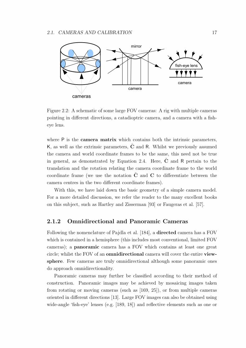
Figure 2.2: A schematic of some large FOV cameras: A rig with multiple cameras
pointing in different directions, a catadioptric camera, and a camera with a fish-
eye lens.
where P is the camera matrix which contains both the intrinsic parameters,
K, as well as the extrinsic parameters, C and R. Whilst we previously assumed
the camera and world coordinate frames to be the same, this need not be true
in general, as demonstrated by Equation 2.4. Here, C and R pertain to the
translation and the rotation relating the camera coordinate frame to the world
coordinate frame (we use the notation C and C to differentiate between the
camera centres in the two different coordinate frames).
With this, we have laid down the basic geometry of a simple camera model.
For a more detailed discussion, we refer the reader to the many excellent books
on this subject, such as Hartley and Zisserman [93] or Faugeras et al. [57].
2.1.2 Omnidirectional and Panoramic Cameras
Following the nomenclature of Pajdla et al. [184], a directed camera has a FOV
which is contained in a hemisphere (this includes most conventional, limited FOV
cameras); a panoramic camera has a FOV which contains at least one great
circle; whilst the FOV of an omnidirectional camera will cover the entire view-
sphere. Few cameras are truly omnidirectional although some panoramic ones
do approach omnidirectionality.
Panoramic cameras may further be classified according to their method of
construction. Panoramic images may be achieved by mosaicing images taken
from rotating or moving cameras (such as [169, 25]), or from multiple cameras
oriented in different directions [13]. Large FOV images can also be obtained using
wide-angle ‘fish-eye’ lenses (e.g. [189, 18]) and reflective elements such as one or
18 CHAPTER 2. CAMERAS, IMAGES AND IMAGE MOTION
more mirrors ([36, 171]). Cameras using a combination of lenses and mirrors are
called catadioptric. Figure 2.2 illustrates the setup of some of these cameras.
Cameras may also be categorized as central or non-central. In central
cameras, which are also known as single viewpoint cameras, all rays of light
entering the camera will intersect at a single point. This is not the case with
non-central cameras, leading to images that appear distorted to humans. Central
cameras also lead to simpler analysis, and most computer vision algorithms are
designed for use with the perspectively correct images that may be obtained from
central cameras.
In practice however, central cameras with very large FOV are more difficult
to build compared to non-central ones. Hence some large FOV cameras are only
approximately central, in that the light rays entering the camera intersect at
approximately a single point (see also [52]). For example, to achieve a FOV
covering 75% of the view-sphere, the Ladybug multi-camera rig [187] consists of
six cameras pointing in different directions, and these are mounted such that the
projection centres of each of the six constituent cameras are close to each other,
resulting in an approximately central camera.
In this work, we focus on central cameras - that is, we assume the camera
may be modeled as having a single, finite, constant, camera centre. The pinhole
camera discussed previously models central, narrow FOV cameras. However, its
equations may also be adapted for use in central, large FOV cameras, where the
camera matrix, P , is still a mapping from the direction of a 3D scene point to
a 2D image point (albeit a more complicated one). For example, Pajdla et al.
[184] derives the camera matrix for central, catadioptric camera systems where
hyperbolic and parabolic mirrors are used to reflect light onto a conventional
camera.
We refer the reader to books such as [24] for an in depth treatment of the
subject.
2.1.3 Camera Calibration
In this work, we assume that cameras have been calibrated - that is, given an im-
age point, some set of calibration parameters will allow us to obtain the direction
of a ray joining the camera centre and the scene point.
Calibration recovers the intrinsic parameters (and extrinsic parameters if the
camera coordinate frame is not aligned with the world frame). Calibration meth-
ods may be loosely classified into two categories. The first involves the use of
2.1. CAMERAS AND CALIBRATION 19
a calibration object, which is an object with certain geometrical properties that
are known a priori, for example, a checkerboard pattern with known dimensions.
The second category does not require calibration objects, using instead, the geo-
metric properties inherent in scene features. For example, vanishing points and
the absolute conic may be used to recover the intrinsics.
Many calibration techniques are available, such as the DLT method [93, 266],
the methods of Tsai [246], of Zhang [278] and many others [88, 121, 97, 160, 242,
188] which can be found in reviews such as [72, 203, 279].
In addition, calibration methods developed specifically for central, large FOV
cameras include [273, 275, 274, 161, 269, 75, 73, 122], whilst works such as [162,
79, 222, 186, 198] deal with non-central and more generic camera systems.
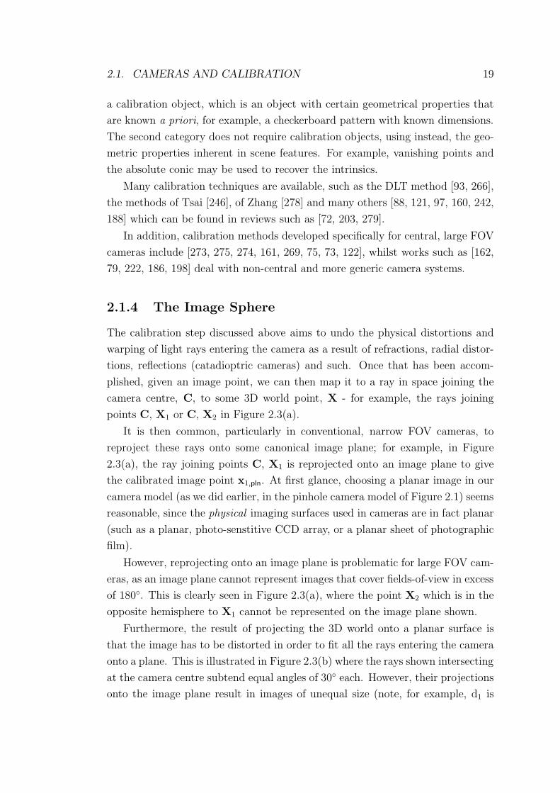
2.1.4 The Image Sphere
The calibration step discussed above aims to undo the physical distortions and
warping of light rays entering the camera as a result of refractions, radial distor-
tions, reflections (catadioptric cameras) and such. Once that has been accom-
plished, given an image point, we can then map it to a ray in space joining the
camera centre, C, to some 3D world point, X - for example, the rays joining
points C, X1 or C, X2 in Figure 2.3(a).
It is then common, particularly in conventional, narrow FOV cameras, to
reproject these rays onto some canonical image plane; for example, in Figure
2.3(a), the ray joining points C, X1 is reprojected onto an image plane to give
the calibrated image point x1,pln. At first glance, choosing a planar image in our
camera model (as we did earlier, in the pinhole camera model of Figure 2.1) seems
reasonable, since the physical imaging surfaces used in cameras are in fact planar
(such as a planar, photo-senstitive CCD array, or a planar sheet of photographic
film).
However, reprojecting onto an image plane is problematic for large FOV cam-
eras, as an image plane cannot represent images that cover fields-of-view in excess
of 180◦. This is clearly seen in Figure 2.3(a), where the point X2 which is in the
opposite hemisphere to X1 cannot be represented on the image plane shown.
Furthermore, the result of projecting the 3D world onto a planar surface is
that the image has to be distorted in order to fit all the rays entering the camera
onto a plane. This is illustrated in Figure 2.3(b) where the rays shown intersecting
at the camera centre subtend equal angles of 30◦ each. However, their projections
onto the image plane result in images of unequal size (note, for example, d1 is
20 CHAPTER 2. CAMERAS, IMAGES AND IMAGE MOTION
(a) (b)
Figure 2.3: Image sphere versus the image plane: (a) X1 is the world point
projecting onto the camera centre C. x1,pln is the image of that point on the image
plane, whilst x1,sph is the image if an image sphere was used. The image plane
is unable to represent points in the opposite hemisphere, such as X2, whereas
the image sphere has no problem with this. (b) The perspective distortion on an
image plane. The visual angles marked out are the same but their projections
onto the image plane are of a different size.
larger than d2). The effects of this distortion of visual angles are most obvious at
the edges of the image and are particularly severe as the camera FOV approaches
180◦.
This leads us to the concept of an image sphere, where the calibrated rays
are reprojected onto some canonical, spherical imaging surface instead of an image
plane. For the calibrated ray, Equation 2.4 becomes:
x =X
|X|(2.5)
where x is the ray or direction vector joining camera centre and the 3D scene
point, X. Another way of thinking about this is to imagine the image point x as
a point lying on the surface of a unit sphere such that x2 + y2 + z2 = 1.
Unlike the image plane, the image sphere naturally represents points over the
entire viewsphere (e.g. in Figure 2.3(a), both the world points X1 and X2 project
onto the image sphere to give the image points x1,sph and x2,sph). Furthermore, the
problem of distorted visual angles does not occur for such a spherical projection.
In general, the image sphere gives a simple framework in which to think about
the problem and, as this thesis will show, has certain nice properties which will

2.2. MEASURES OF IMAGE MOTION 21
aid us in the task of egomotion estimation.
In this work, we focus on calibrated, central cameras, and image points can
generally be assumed to satisfy Equation 2.5, unless it is clear from the context
that this is not the case (e.g. when dealing with uncalibrated cameras). We also
refer to the image point x and the ray in the direction of x interchangeably.
2.2 Measures of Image Motion
Taxonomy
Consider two or more images of a scene taken by a moving camera. Given a point
in one image, we wish to identify the same point in a different image - that is,
the two matching image points should correspond to the same world point. This
is known as the correspondence problem.
Decades of research have yielded a plethora of algorithms for measuring image
motion and for solving the correspondence problem. In our review, we categorize
them as optical flow algorithms and point correspondence methods.
Optical flow methods typically estimate image motion from constraints on the
spatiotemporal variations of image intensity. These methods are often used to
compute image motion densely over the entire image, often represented as a field
of image motion vectors known as the optical flow field (e.g. Figure 2.4).
Meanwhile, point correspondence methods attempt to obtain a robust and
discriminative signature from the intensity gradient patterns in the neighbour-
hood of an image point. This signature is called a feature descriptor and should
be discriminative enough for that image point to be correctly matched with the
corresponding point in a second image.
The key difference between the two classes of methods is that most optical
flow methods make approximations (e.g. the brightness constancy assumption,
see Section 2.2.1) that limit the range of motion sizes they can handle, whereas
point correspondence methods do not do so. This means that in practice, optical
flow methods are typically more suited to smaller image motions. In contrast,
point correspondence methods work robustly even under large image motions
(which may result, for example, from large camera translations and rotations).
Representations of Image Motion
There are two ways by which image motion may be represented:
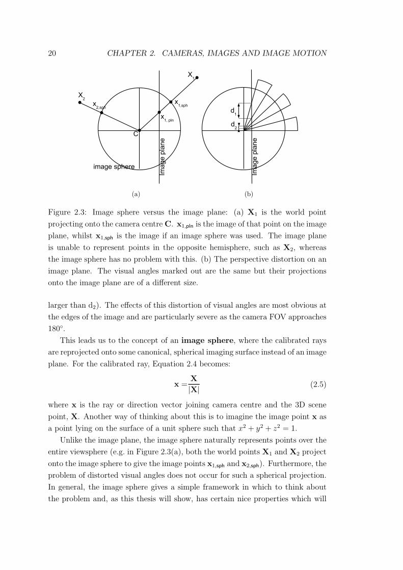
22 CHAPTER 2. CAMERAS, IMAGES AND IMAGE MOTION
(a) (b)
Figure 2.4: (a) A forward moving observer sees a diverging optical flow field. As
the observer moves, almost every image point will undergo some motion, leading
to an array of optical flow vectors, where each vector starts at the original position
of the image point and terminates at its new position. The dot indicates the focus
of expansion. (b) Flow on an image sphere. The large arrow indicates the focus
of expansion.
• the image coordinates of the point before and after moving, or
• the vector difference between those coordinates
The latter may be plotted on the image to give a vector field called the optical
flow field. Figure 2.4(a) shows the flow on the image plane whilst Figure 2.4(b)
illustrates flow on the image sphere.
In the literature, the term ‘optical flow’ is sometimes used to refer to the class
of dense optic flow algorithms; and at other times, used to refer to the vector
field representation of image motion. The nomenclature used by researchers is
somewhat confusing because the vector field representation may actually be used
for image motion measured with algorithms from either the dense optic flow or
the point correspondence categories.
In practice, if the image motion is small, both dense optic flow algorithms
and point correspondence methods will work, and the outputs of both types of
methods may be represented with the vector field representation of flow. However,
if the image motion is fairly large, only point correspondence methods are used
because of their robustness to scale, orientation and other changes in the image.
The dense optic flow algorithms do not handle large image motions well, and the
vector field representation may break down (for example, if the camera were to

2.2. MEASURES OF IMAGE MOTION 23
(a) (b)
Figure 2.5: The aperture problem. (a) The motion of points on a moving bar
appears to be v when viewed through the circular aperture. (b) However, if the
entire bar was visible, its actual motion would be v′.
rotate by some angle larger than 90◦, it is not possible to represent the resulting
image motion with the vector field representation).
Ambiguities
It is important to note that the observed motion of image points does not nec-
essarily equate the true motion of the points. This is because image information
is often limited, leading to ambiguities in the estimates of the motion of world
points.
This may be illustrated by a phenomenon known as the aperture problem [250].
Consider Figure 2.5, where a bar appears to move from left to right (direction v)
when viewed through an aperture. However, the true motion of the bar, if the
entire bar was visible, is in fact upwards and to the right (direction v′). When
viewed through the aperture, the observer is only able to measure the component
of motion that is in the direction of the intensity gradient. The component of
motion that is perpendicular to the intensity gradient is not measurable. In the
example, the observed v, is the component of v′ that is perpendicular to the
light-to-dark edge. v is called the normal component of image motion, since it is
normal to the edge.
Furthermore, it is sometimes simply impossible to estimate image motion due

24 CHAPTER 2. CAMERAS, IMAGES AND IMAGE MOTION
to a lack of features or textures in the environment. For example, consider an
attempt to estimate from images, the motion of world points lying on a blank,
white wall. This is unlikely to result in anything useful since an image of the blank
wall would contain insufficient visual information. Likewise, within environments
with repeated structures, points of very similar appearance may easily be confused
with each other, leading to erroneous estimates of motion.
Consequently, due to the ambiguities discussed above, the possibility of error
always exists in egomotion estimates derived from image motion measurements.
In general, however, image motion measurements give a fairly good approximation
of the true motion field.
Next, we will discuss methods from both the optical flow and point corre-
spondence classes, and compare their advantages and disadvantages in order to
understand how they impact the task of egomotion estimation.
2.2.1 Optical Flow Algorithms
Following the taxonomy of Barron et al. [17], we will discuss three major cate-
gories of methods recovering dense optical flow. They are ‘differential methods’,
‘correlation methods’ and ‘frequency methods’.
Methods in the optical flow category typically assume that the image intensity
I(x, t) at an image point x and at the time instant t, is approximately constant
over a short duration and within a small neighbourhood of x (that is, the bright-
ness constancy assumption):
I(x, t) ≈ I(x + δx, t + δt) (2.6)
Taking a first order approximation gives the optical flow constraint equation:
∇I · v + It = 0 (2.7)
where ∇I gives the spatial partial derivatives of intensity, It its temporal deriva-
tive, and v is the optical flow vector. This is a constraint on image motion from
the local spatial intensity gradient about the point x. This equation is ill-posed
[17], since only the component of v that is in the direction of the spatial gradient
can be found - which is the aperture problem discussed previously. To resolve the
ambiguity inherent in the equation, various additional constraints are used, and
we discuss them in the following.
Differential Methods: Local methods only consider the intensity gradient over
a local window. For example, the method of Lucas-Kanade [146] solves Equation
2.2. MEASURES OF IMAGE MOTION 25
2.7 for v via weighted least squares. Chu and Delp [40] and Weber et al. [260]
estimated the flow using total least squares, whilst Bab-Hadiashar and Suter
[12] introduced a more robust solution using what they term weighted-total least
squares.
A more general formulation of the Lucas and Kanade method [14] considers
the problem as that of minimizing:
∑
x
[ I(W (x,p)) − T (x) ]2 (2.8)
where a patch of the image I, in the neighbourhood of point x, is warped under the
function W (with warping parameters p), such that it is aligned with a template
image patch, T (x). This warping can be an affine or similarity transformation,
in which case, the problem is non-linear and may be solved by Gauss-Newton
gradient descent methods.
On the other hand, approaches such as that of Gupta and Kanal [83] side-step
the computation of intensity gradients by using the Gauss divergence theorem to
convert the problem into one of local integration over surfaces and volumes of
intensity.
Global methods generally enforce some notion of global smoothness in addition
to Equation 2.7. Well-known approaches include that of Horn and Schunck [102],
which minimizes a global energy function which is solved from the Euler-Lagrange
equations for the function via the iterative Gauss-Seidel algorithm. Some meth-
ods also relax the brightness constancy assumption to take into account more
general transformations of the flow field [207, 174, 192]. The work of Brox et al.
[30] is a recently proposed coarse-to-fine warping algorithm giving highly accurate
estimates; it is representative of variational methods that combine various con-
straints such as brightness constancy, gradient constancy and various smoothness
terms to estimate flow.
Various other methods also exist, including approaches that obtain flow from
contours and surface models [99, 32, 265], as well as approaches using linearly
independent filters [214, 215].
Frequency Methods: These methods rely on spatiotemporal filters that work
in the Fourier domain. Under certain conditions, these methods can be mathe-
matically equivalent to computing flow from differential methods [213]. The optic
flow for certain types of stimuli are more easily estimated using these methods
compared to other flow approaches [1]; for example, differential and correlation

26 CHAPTER 2. CAMERAS, IMAGES AND IMAGE MOTION
methods would have difficulties with sparse patterns of moving dots. These fre-
quency methods are often used as models of motion sensing in biology.
The methods of Heeger [94] and of Fleet and Jepson [67], estimate flow by
using banks of spatiotemporal Gabor filters (the product of spatiotemporal Gaus-
sian functions with trigonometric functions) tuned to different spatiotemporal
frequencies to find the strongest velocity orientation about an image point. Re-
lated research includes phase-based methods [66, 41, 113], and methods inspired
by the behaviour of motion sensitive cells in the visual cortex [258, 82].
Correlation Methods: Correlation based methods attempt to find matching
image patches by maximizing some similarity measure between them under the
assumption that the image patch has not been overly distorted over a local re-
gion. Such methods may work in cases of high noise and low temporal support
where numerical differentiation methods are not as practical. These methods are
typically used for finding stereo matches for the task of recovering depth from
stereopsis.
Representative work includes that of Sutton et al. [225], which allows a linear
deformation of the matched neighbourhood, and the work of Anandan [6], which
computes the correlation between two patches via Sum-of-Squared-Differences
(SSD) within a coarse-to-fine scheme. Variations on this idea include the work
of [33, 80, 182]. Recent work on correlation-based matching use graph cuts to
enforce spatial consistency whilst taking into account occlusions [26].
Correlation methods are perhaps the predecessors of the point correspondence
class of methods that we will discuss next. Whilst the former typically use SSD,
pixel-differencing and warping functions to establish the correlation between im-
age patches, point correspondence methods extract more robust and discrimina-
tive descriptors from the image patches, leading to much better matching under
large image and camera motions.
2.2.2 Point Correspondence Algorithms
Point correspondence methods seek to recover feature descriptors that summa-
rize the image information in the neighbourhood surrounding an image point.
These descriptors need to be sufficiently discriminative such that the correct
correspondence can be established between the same world point observed in
different images. The feature must discriminate between the correct match and
other potential (but wrong) matches.

2.2. MEASURES OF IMAGE MOTION 27
Since the other image is typically captured after the camera has undergone
some motion, the appearance of the image patch around the point of interest will
have changed due to differences in scale, rotation and illumination. Hence, the
descriptor also needs to be robust to these changes as well as to other sources of
noise.
One may infer from the discussion up till now, that not every part of an image
is conducive for the recovery of features that can be robustly matched or tracked.
Edges are easy to detect but estimates of edge motion may be ambiguous due to
the aperture problem. Nagel [170] showed that image points with high Gaussian
curvature - often corresponding to corner or junction points - allow the recovery
of full image motion (not just the normal component).
The Moravec interest point detector [166] and the Harris corner detector [85]
were some of the earliest investigations into image points that could be recovered
repeatably. Zhang et al. [280] placed an additional correlation window around
Harris corners and showed that such points could be tracked over fairly large
camera motions. This was perhaps the precursor to the idea of feature descriptors.
Schmid and Mohr [206] used a rotationally invariant window instead of the regular
correlation window for matching Harris points.
This was followed by the introduction of the Scale-Invariant Feature Trans-
form (SIFT) descriptor [144, 145] that was invariant to rotation, scale and illumi-
nation changes. Features that were invariant to affine deformations soon followed
[19, 164, 248], leading to successful matching even for image patches suffering
fairly large perspective foreshortening effects. Maximally-Stable Extremal Re-
gions (MSER) [157] are another example of features that are robust and stable
over large camera motions.
Key issues for these point correspondence algorithms are the computational
overhead as well as the sparsity of the computed interest points. Speeded-Up
Robust Features (SURF) [21] used integral images to reduce the computational
time needed for performing multiple Gaussian convolutions on the input intensity
image. More recently, the DAISY descriptor [236] represents a step towards fast,
densely computed features. However, although DAISY was designed for efficient
dense computation, the problem of quickly matching the large numbers of features
found remains a challenge.
In the following, we discuss the various components often occurring in point
correspondence algorithms:
Feature Descriptors: Point correspondence algorithms typically compute
descriptors from local image structures such as the intensity gradients in the

28 CHAPTER 2. CAMERAS, IMAGES AND IMAGE MOTION
vicinity of a feature point. The SIFT algorithm for example, parcels out the
local neighbourhood of the point into several square sub-windows, within which
the orientations of intensity gradient edges are computed. These observations
contribute to a series of histograms which encode the local intensity gradient
structure of the point in a robust manner. The resulting histograms are concate-
nated as a feature vector, which form a discriminative signature of that point. To
match the point with potential correspondences, some similarity measure (such
as the Euclidean distance) is found between the feature vectors, and the most
similar one will be the correct match.
Rotation Invariance: In a different view of the scene, certain parts of the
image may have rotated relative to the reference image. The square windows
used in the SIFT or SURF algorithms would then straddle slightly different im-
age regions and the descriptors computed may differ quite significantly from the
descriptors found in the reference image.
To compensate for rotation, point correspondence methods usually recover
a dominant orientation for each feature point in the reference image, based on
some robust average of the orientations of the local intensity gradients. In the
new image, a rotation of some image object would result in a rotation of the
local dominant orientation as well, and the feature descriptor can then be com-
puted with respect to this orientation. This leads to the rotational invariance of
descriptors and results in better matching.
Scale Invariance: In order to match regions of interest, the scale of the
region needs to be considered as well. When an object is viewed up close, it
occupies a larger area on the image, and the object structure is seen in greater
detail. However, as the camera backs away, the image area occupied by the object
shrinks and the details on the object are blurred. Scale invariance is the ability
to match an image patch with a corresponding patch which is at a different scale.
In order to achieve scale invariance, one approach is to search for points that
are robust to scale changes in image space and in scale space. Scale space [264]
consists of the collection of images at varying scales (like a set of images taken
under various levels of ‘zoom’ or magnification). To obtain this, an image is
convolved with Gaussian kernels of progressively increasing standard deviation.
The blurring introduced by the Gaussian convolution simulates the destruction
of detail arising from a decrease in scale [124, 139].
The SIFT algorithm locates local maxima and minima points in scale-space by
searching a pyramid of Difference-of-Gaussian (DoG) images (that is, a stack of
images blurred under Gaussian kernels of increasing standard deviation, which is

2.2. MEASURES OF IMAGE MOTION 29
then subtracted with an image of a neighbouring scale). This is an approximation
of the scale-normalized Laplacian-of-Gaussian which is necessary for true scale
invariance [139]. These local scale-space optima points tend to make very stable
image features [164].
The DAISY feature [236] takes an alternative approach by considering a multi-
scale feature, rather than a scale-invariant one. There, the feature descriptor is
found at a range of scales, leading to a higher dimension feature compared to
that of the SIFT descriptor. This approach is also reported to successfully match
feature points that have undergone changes in scale.
2.2.3 Which Method to Use?
The main advantage of optical flow methods is that they can be computed densely
over the entire image quite quickly compared to point correspondence methods.
However, the accuracy of their estimates are typically worse than those of point
correspondence methods. Furthermore, many optical flow methods rely on as-
sumptions such as brightness constancy (Equation 2.7) which only hold under
certain conditions (and the error is worse when these conditions are not met).
Therefore, a practical system must consider various issues (such as the trade-off
between processing time and accuracy) when choosing which class of methods to
employ.
Density of estimates. Egomotion can be recovered from a small set of
accurately recovered correspondences or optical flow. For example, a minimum of
five points is sufficient for recovering the three parameters of camera rotation and
two parameters of translation (see Chapter 3). However, in many applications,
recovering egomotion is not the end of the story: after egomotion is found, it
may be necessary to then compute a depth map, which would require a dense
computation of image motion.
Accuracy. Whilst optical flow methods are typically less accurate, many
applications do not necessarily require highly accurate optic flow. Robot naviga-
tion is possible without the sub-pixel accuracy of point correspondence motion
estimates and navigation from qualitative (rather than quantitative) measures
of flow is even possible. On the other hand, the reconstruction of scenes for
movie post-production purposes or 3D modeling, requires highly accurate image
motion estimates, and point correspondence methods which are both accurate
and densely computed (such as DAISY) may be more suitable. Moreover, re-
cent advances in dense, optical flow methods (for example, Brox et al. [30]) have

30 CHAPTER 2. CAMERAS, IMAGES AND IMAGE MOTION
accuracies approaching those of point correspondence approaches.
Speed. Whilst the DAISY feature is designed for fast and dense computa-
tion, matching these features remains a slow process. The discriminative power
of features exacts a price in the form of the high dimension of the feature vectors.
To perform matching, some distance or similarity measure has to be calculated
between many high-dimensional feature vectors. As a result, it is not possible
at present, to obtain dense and fast point correspondence estimates of image
motion. Sparse point correspondence methods, however, may be computed in
real-time but this requires special hardware. For example, SIFT features may be
found at high speeds using Graphical Processing Units (GPUs), which are highly
parallelized processors adapted for graphics applications [268].
Motion Size. Perhaps the most marked difference between the point corre-
spondence and optical flow methods is the size of the image motion considered.
Optical flow methods work for small motions and hierarchical or multi-scale ex-
tensions of these methods can work for somewhat larger image motions. However,
when the motions are large enough that the local image regions undergo signifi-
cant affine and perspective distortions or changes in scale, these methods generally
tend to break down. Point correspondence methods, however, work robustly for
small image motions as well as large ones (up to a point, of course), due to the
reasons discussed earlier.
Conditions Apply... Those optical flow methods that solve for flow from
Equation 2.7 rely on the assumption of brightness constancy. This assumption
holds under: (1) (locally) uniform scene illumination, (2) Lambertian surface
reflectance, (3) orthographic projection and (4) pure translation parallel to the
image plane (see [17]). However, some of the optical flow methods discussed pre-
viously are exempt, for example Lucas-Kanade under an affine warping model
[14], as well as the methods of [207, 174, 192]. On the other hand, point cor-
respondence methods are more robust in general, and tend to perform well in
general conditions without any of these restrictions.
In the experiments conducted as part of this work, the size of the image mo-
tion was the main consideration for our choice of the image motion measurement
algorithms used. For small image motions (corresponding to experiments involv-
ing small camera motions in Part II) we found the Lucas-Kanade optical flow
method to be very useful. Meanwhile, experiments involving mainly large image
motions (Part III) generally used SIFT features. The other methods discussed
in this chapter are equally valid choices and may be substituted, subject to the

2.3. SUMMARY 31
various system criteria (speed, accuracy etc) mentioned above.
2.3 Summary
Beginning with the pinhole camera model, we described the process by which
world points project to image points within a camera. These image points may
be represented as lying on 2D surfaces such as planes or spheres - with the latter
representation having various advantages, such as being more suitable for large
FOV images.
We then considered the phenomenon of image motion which arises when the
camera and the world points move relative to each other. We also surveyed a
number of algorithms for measuring image motion, which were categorized into
optical flow methods and point correspondence approaches.


Chapter 3
Review of Egomotion Recovery
3.1 Egomotion Estimation
In the last chapter, we considered the geometry of cameras and image formation,
and various methods by which the motion of image points may be measured.
Now, we will look at one of the major mechanisms causing image motion - that
is, the motion of the camera itself. We consider the equations governing the
geometrical effects of camera motion upon image motion, and look at various
approaches to estimating camera egomotion.
Egomotion recovery is a classical problem and the last few decades have seen
intensive research in this area. The general problem of self-motion estimation may
be solved using visual and non-visual means (such as measurements made by Iner-
tial Motion Units (IMUs), Global Positioning System devices (GPS), sonar, radar,
laser range-finders and such). Even with vision, there are multiple approaches
ranging from systems using a single camera (monocular), a pair of stereo cameras
(binocular), a network of cameras (n-ocular), cameras attached with time-of-flight
sensors (which estimate scene depth), or even cameras operating in the non-visible
spectrum.
In this thesis, we focus on monocular, visual images in the visible spectrum.
We summarize the characteristics and assumptions of our approach below:
• a moving monocular camera
• estimate from two camera views1
• a single camera centre
1This also implies that no knowledge of the past state of the camera is assumed.
33

34 CHAPTER 3. REVIEW OF EGOMOTION RECOVERY
• calibrated camera
• using image motion measurements2
• unknown scene depth
• rigid body motion (characterized fully by a translation and rotation)
3.1.1 On the Size of Camera Motions
Existing egomotion recovery research may be categorized into two classes - those
assuming differential camera motion and those assuming discrete camera motions.
Differential motion methods assume that the camera undergoes an instantaneous
translational velocity and an instantaneous angular velocity (i.e. rotation). The
discrete motion methods, on the other hand, assume that the translation and
rotation between successive views is large.
If the motion is large, the instantaneous methods become less accurate and
eventually break down. It was previously accepted that if the motion was too
small, then the discrete methods may also become less accurate. However, some
recent research seems to suggest that certain discrete motion methods may work
well even for small motions [138, 152, 119, 243, 20]. For example, Lin et al. [138]
showed theoretically (under certain conditions and assuming a proportional noise
model) that the discrete motion algorithm they considered performed well for
both discrete and differential motions.
In general, the choice of using discrete or differential algorithms is often de-
cided by the target application considered. Certain applications consider views
taken from cameras that are far apart, and the discrete motion methods are more
suitable. On the other hand, many applications involving cameras that are mov-
ing (e.g. mounted on a car, robot, or person) would be well-suited to the use of
differential motion methods.
However, in the latter case of moving cameras, it must be noted that since all
cameras have a finite frame-rate (rate at which images are captured), the motion
undergone between two successive frames would be small, but never truly differ-
ential (as the camera would have moved a finite distance in the time between
the capture of one image and that of the next image). Therefore, many appli-
cations may in fact find themselves operating in conditions that are somewhere
2We assume that the image motion observations are a good approximation of the true motion
field.

3.1. EGOMOTION ESTIMATION 35
in between strictly discrete or strictly differential motions. In practice, there is a
range of motion sizes (not too large and not too small) for which both methods
work comparably. Comparisons between the operating range of some discrete
and differential motion methods can be seen in work such as [138, 221, 255, 148].
Since these discrete and differential camera egomotion estimation algorithms
take image motion measurements as their inputs, the size of the camera motions
also impacts which image motion method to use. Large camera translations and
rotations typically result in large image motions which need to be measured with
point correspondence methods. Conversely, small camera motions tend to give
rise to small image motions, which may be measured with either optical flow or
point correspondence methods (and the factors affecting one’s choice are discussed
in Section 2.2.3, page 29).
In the early days of computer vision, only small image motions could be
automatically measured, using the optical flow techniques that were available at
the time. This perhaps explains the focus then on differential motion methods,
which resulted in papers such as [31, 281, 120, 191, 114, 199, 100, 190, 237, 173,
103, 63, 212, 220, 4, 112, 272, 130, 228, 2, 159]. However, the introduction of point
correspondence measures of image motion enabled image points to be matched
even under large camera translations and rotations. This suddenly made discrete
motion methods practical (previously, researchers had to virtually hand mark
point matches when the images were too different for optical flow methods to
work) and the last decade has seen much interest and research in discrete motion
methods (such as [141, 247, 262, 87, 181, 136, 93, 277, 147, 86, 59, 181, 136, 179,
89, 90, 91, 117]).
In this chapter, we will discuss the various algorithms and methods that have
been devised for egomotion recovery in the last three or four decades.
3.1.2 On Differential Motion Algorithms
Without loss of generality, let the camera centre be the origin of both the world
and camera coordinate frames, and assume unit camera focal length. Then, the
equation relating optical flow and egomotion under perspective projection onto
a planar image by a pinhole camera model, was derived by Longuet-Higgins and
Prazdny [142] to be:
x(x) =
[
1 0 − x1
0 1 − x2
]
( t
|X|+ w × x
)
(3.1)

36 CHAPTER 3. REVIEW OF EGOMOTION RECOVERY
where x(x) is the optical flow at an image point, x = [x1 x2 1]T , and the depth of
the corresponding scene point is |X|. t is the camera translation, w is the camera
rotation3, and × denotes the vector cross product.
Under the spherical image representation, with the spherical image point,
r = [rx ry rz]T , such that r2
x + r2y + r2
z = 1, we have [190]:
r(r) =1
| R |((t · r)r − t) − w × r (3.2)
where we use r (radius) instead of x to emphasize the difference between Equa-
tions 3.2 and 3.1, that is, the image point in 3.2 resides on the image sphere. (To
keep the notation self-consistent, we also denote the scene point as R instead of
X.)
As before, the point r on the unit image sphere has the same direction as a
ray joining the camera centre and the scene point (which is at a distance of |R|
units away). Hence, we will use the spherical image point r and the ray in the
direction r interchangeably, in our discussions.
These equations (3.1 and 3.2) are essentially a first-order Taylor approxima-
tion of the geometrical effects of egomotion on the perceived image motion [221].
This linearization is possible because the nonlinearities of these effects are in-
significant when the size of camera translation and rotation is small. However, if
camera motion increases, the approximation becomes less accurate and eventually
breaks down. These methods are therefore limited to scenarios where camera mo-
tions are small, and under larger camera motions, the discrete motion techniques
described in Section 3.1.3 should be used instead.
Scale Ambiguity
The are a total of 7 unknowns in Equation 3.2 (and also 3.1). The depth, |R|,
is 1 unknown. Rotation, w, has 3 unknowns. The translation, t, also has 3
unknowns. However, with only image motion information, we can only recover
2 of the 3 parameters of translation. This is due to an ambiguity in the scale of
the translation.
Consider the first term in Equation 3.2. We can factor out the magnitude of
the translation vector to get∣
∣
tR
∣
∣((t·r)r−t). The∣
∣
tR
∣
∣ factor shows that the scale of
translation is ambiguous: a larger translation and correspondingly smaller depth
3Using the Euler axis-angle representation, where w is the rotation axis and |w| is the
rotation angle.

3.1. EGOMOTION ESTIMATION 37
can give rise to the same image motion observation as a smaller translation and
correspondingly larger depth.
As a result, only 6 out of the 7 unknown parameters can be recovered - 5 are
parameters of motion (3 for rotation, 2 for translation) and 1 is the unknown scene
depth. Egomotion recovery involves finding the 5 motion parameters. Once that
has been found, depth can be estimated - up to a scale as well - which is variously
termed as relative scene depth, scaled depth or sometimes time-to-contact (since
the inverse of∣
∣
tR
∣
∣ has units in time).
Differential: Decoupling of Motion Components
As discussed above, under the assumption of differential camera motion, the first-
order approximation of the relationship between egomotion and image motion is
described in Equations 3.1 and 3.2. From inspection, we see that under this
approximation, the two equations are linear in translation and in rotation. This
means that it is not difficult to decouple the estimation of translation from the
recovery of rotation with some algebraic manipulation. Many of the algorithms
which we will discuss next take advantage of this to split up the problem so that
translation and rotation may be separately estimated.
Algorithms
A straightforward least squares solution to Equation 3.1 or 3.2 is impossible since
scene depth, R, is a function of r. Therefore, every additional flow observation
introduces an extra constraint, but also an extra unknown in depth, so that the
system of equations is under-constrained.
The approaches of Bruss and Horn [31] and of Maclean et al. [150] remove
the dependence on depth algebraically. For example, taking a dot product with
(t × r) on both sides of the egomotion equation gives us an equation bilinear in
t and w:
(t × r) · r =1
| R |(t × r) · ((t · r)r− t) − (t × r) · (w × r)
⇒ (t × r) · r = − (t × r) · (w × r)
(3.3)
A least squares estimate of rotation can then be found as a function of translation.
Back-substitution into the equation gives a nonlinear equation for translation
which can be solved by nonlinear numerical optimization.
Another nonlinear approach is that of Prazdny [190], which obtains a set of
3rd order polynomials by algebraically removing translation from Equation 3.2.

38 CHAPTER 3. REVIEW OF EGOMOTION RECOVERY
It is found that rotation can be constrained from a triplet of points via:
n3 · (n1 × n2) = 0, where ni = (w × ri + ri) × ri (3.4)
Tomasi and Shi [237] proposed a different constraint on motion which uses
the angle between any two rays corresponding to two image points ri and rj. The
measured angle between two rays changes as the camera moves and the image
is said to deform. This measure of image motion is rotationally invariant as a
purely rotational movement will preserve the angle between two rays. With this
approach, equations that are bilinear in translation and scene depth at the two
points are obtained. Once again the resulting equations are solved by nonlinear
methods.
Another constraint comes from the observation that image points which are
close to each other will have nearly similar rotational components, but their
translational components can be quite different if the depths at the two points
are different (this is easy to see from Equation 3.2) [190]. This corresponds to
neighbouring points that straddle a depth discontinuity. Subtracting the flow at
two such points eliminates the rotational component and the remaining terms
depend purely on translation. This same observation spawned a number of ap-
proaches, both classic [199, 100] and recent [105].
However, Prazdny [191] also observed that in general, adding or subtracting
the flow at two or more points in some special way (not necessarily at a depth
discontinuity), can result in the rotational components canceling out and leaving
a constraint on translation. Linear subspace methods achieve this by a linear
combination of flow vectors with appropriately chosen weights. How these weights
are computed is detailed in the works of Jepson and Heeger [114, 115].
The differential epipolar constraint is the differential motion analogue to the
epipolar constraint used in discrete motions (which we discuss in the next section).
Kanatani et al. [118, 120] and Zhuang et al. [281] used the differential epipolar
constraint to linearly solve for the flow fundamental matrix, which encapsulates
the translation and rotation parameters.
More recently, Stewenius et al. [221] presented a nonlinear minimal solver4
for the problem, known as the infinitesimal (or differential) five-point algorithm.
The idea is that the direction of translation, a point and the de-rotated optical
flow vector at that point all lie on the same plane. Rearranging Equation 3.2, we
4i.e. requiring the minimal number of points (5 points) to solve for the 5 unknown motion
parameters (translation found up to a scale) in a calibrated camera.

3.1. EGOMOTION ESTIMATION 39
have the de-rotated flow:
m =1
| R |((t · r)r− t) = r + w × r (3.5)
Due to coplanarity, we have:
t · (r× m) = 0
⇒ tT [r]×
[
[r]× r]
[
w
1
]
= 0
⇒ ai
[
w
1
]
= 0
(3.6)
where ai is a 1 × 4 row vector. Five observations (i = 1 · · ·5) will give five
equations which may be stacked into a matrix A = [a1 · · ·a5]T . From rank-
nullity constraints, the five sub-determinants of A must vanish. A tenth degree
polynomial is obtained and solved, using either Grobner basis or Sturm sequence
based root solvers.
Recognizing the ambiguity in optic flow measurements due to the aperture
problem, so-called ‘direct’ estimation methods use the ‘normal flow’ (that is, the
component of flow in the direction of the intensity gradient; see Section 2.2, page
23) instead of full optical flow. The normal flow may be observed directly from
the spatiotemporal gradients of brightness and is less challenging to find. These
direct methods include the work of [172, 173, 103, 63, 60, 62, 211, 212, 220].
Among these, [63, 60, 62, 211, 212] solve the problem by imposing constraints
from normal flow that reduce the motion solutions to some restricted subspace.
Koenderink and van Doorn [125, 126] investigated the use of divergence, curl
and shear deformations of the optic flow field, in order to extract invariant prop-
erties in the camera motion and scene surface shape. Using these results, first
and second order image motion flow fields were used in methods proposed by
[190, 259] to solve for motion in scenes involving rigidly planar surfaces.
Sequential algorithms suggest using multiple images filtered temporally to
estimate motion. Unlike the other methods mentioned in this thesis, this ap-
proach generally requires more than two views of the scene. Extended Kalman
filtering methods were proposed by [29, 58, 5, 158, 95, 96]. An initial guess of
the parameters is updated in these schemes until it converges. Particle filtering
and sequential monte-carlo approaches include the work of [219, 193, 194] and a
review may be found at [3].
There are also methods which take a qualitative approach rather than a quan-
titative one [63, 252]. For example, the Focus of Expansion of the flow field can

40 CHAPTER 3. REVIEW OF EGOMOTION RECOVERY
be detected qualitatively. It is not unreasonable then, for translation and rotation
to be found from qualitative measurements also.
Other methods of note include those using Hough-like voting [15], those relying
on the depth-positivity constraint [28], those using fixation to simplify motion
estimation [61, 229, 47], as well as the work of [4, 112, 272, 130, 228, 2, 159] and
a great many more, which can be found in reviews such as [235].
3.1.3 On Discrete Motion Algorithms
Figure 3.1: The epipolar plane.
Early work on discrete camera motion is represented by works such as Ull-
man [250] or Roach and Aggarwal [200]. However, it was the classic paper of
Longuet-Higgins [141] that introduced the epipolar constraint on which most dis-
crete motion algorithms are based (such as [247, 262, 141, 87, 181, 136]).
The geometry of the epipolar constraint may be understood as follows. Given
two views of the scene which are related by some rigid motion, the two camera
centres C and C′ and any scene point seen by both cameras will lie on the same
plane, termed the epipolar plane (given by the dotted lines in Figure 3.1). The
observations are correspondences between image points x and x′. The translation
vector t =−−→CC′ intersects the image plane at the epipoles e and e′.
From the coplanarity condition, the epipolar constraint equation can be de-
rived to be [93]:
x′TFx = 0, where F = K
′−TEK
−1 (3.7)
F is the fundamental matrix which encapsulates calibration and motion param-
eters; K and K′ are the calibration matrices of the two cameras; and E is the
essential matrix. The essential matrix describes only the motion - translation t

3.1. EGOMOTION ESTIMATION 41
and rotation R - of the camera:
E = [t]×R (3.8)
(R is the matrix representation of rotation whereas w, which previously appeared,
uses the axis-angle representation.) Recovering F or E becomes a linear problem
using the epipolar constraint.
For uncalibrated cameras, the fundamental matrix may be recovered by the
eight-point algorithm of Longuet-Higgins [141], Hartley’s normalized eight-point
algorithm [87] or other similar variants [168, 39]. Each point correspondence
gives a linear constraint, and eight or more points gives a unique solution for F
which may be found by linear least-squares via methods such as Singular Value
Decomposition (SVD). Alternatively, if an additional singularity constraint is
enforced, a minimum of seven points may give a solution via the nonlinear seven-
point algorithm (which yields 3 solutions) [93]. Other variations on these exist
(see reviews [277, 147]), but all are based on the same principle of the epipolar
constraint.
In the calibrated case (which is our focus), the essential matrix may be re-
covered from a minimum of five point correspondences [86, 59] using the 5-point
algorithms of Nister [181, 179], Li and Hartley [136] or Kukelova et al. [129]. These
five-point algorithms involve a nonlinear solution where the roots of a tenth order
polynomial are found using methods based on Guass-Jordan elimination, Grobner
basis techniques and such.
The discrete motion methods mentioned so far minimize the algebraic distance,
that is, they minimize the L2 norm of ||Ah|| (Equation 3.7 can be expressed in
the form Ah where A contains the entries of F, and h is a vector containing cross-
terms of the xyz-components of vectors x and x′). The advantage of using the
algebraic distance is that the resulting cost function admits a linear solution (if
8 or more points are used). However, its disadvantage is that minimizing the
algebraic distance is not geometrically meaningful [93].
As a result, for greater accuracy and optimality, the estimate from one of
the above methods is often used to initialize a second, refinement stage which is
instead based on minimizing the geometric distance, which in this problem is the
reprojection error:∑
i
[d(xi, xi)2 + d(x′
i, x′
i)2] (3.9)
where xi and x′
i are the ‘true’ point correspondences that satisfy the epipolar
constraint exactly. This is a maximum-likelihood estimate under the Gaussian
42 CHAPTER 3. REVIEW OF EGOMOTION RECOVERY
noise assumption and can be solved using iterative Levenberg-Marquardt and
other bundle adjustment methods. Due to the nonlinear cost function, these
methods converge on local minima, hence a good initialization is necessary. We
refer the reader to [93, 245] for a detailed treatment.
More recently, research has considered globally optimal methods of minimizing
cost functions based on the L∞ norm rather than the L2 norm. With known
rotation, translation can then be found optimally under the L∞ norm, using
Second Order Cone Programming (SOCP) [91, 117]. Hartley and Kahl [89, 90]
later showed that it is possible to optimally solve for both translation and rotation
by a search strategy based on the branch and bound algorithm.
Note that within the literature, the problem of recovering discrete camera
motion is variously called the ‘relative pose’ or the ‘relative orientation’ problem.
These terms are used in order to include the more general problem of two different,
stationary cameras observing the scene, instead of the problem of a single, moving
camera observing the scene at two time instances. When there are multiple
cameras, the calibration parameters, and hence the fundamental matrix may
vary across cameras. However, for the case of calibrated cameras, this difference
is not important and the relative pose and egomotion estimation problems are
effectively equivalent.
Discrete: The Coupling of Translation and Rotation
We earlier saw that in the case of differential camera motion, the image motion
could be approximated as a linear function of camera translation and rotation.
However, in the case of discrete or large motions, Equations 3.1 and 3.2 no longer
hold, and we instead use the epipolar equation, Equation 3.7, to constrain camera
motion.
Under discrete camera motion, we see that the translational and rotational
components of motion are coupled together in the essential or fundamental ma-
trices. In particular, the function is bilinear in translation and rotation, i.e.
E = [t]×R. As a result, the various ‘tricks’ used in differential egomotion algo-
rithms for eliminating translation and first solving for rotation, or vice-versa, will
not work here. Therefore, attempting to decouple the translation and rotation in
order to obtain linear constraints on translation and rotation is non-trivial and

3.1. EGOMOTION ESTIMATION 43
was not possible up till now5.
In Chapter 7 we will derive linear constraints on translation that are inde-
pendent of rotation, and separately, linear constraints on rotation independent
of translation. We demonstrate that under the special condition of antipodal
points, the generally nonlinear/bilinear problem is decoupled to become linear in
translation and linear in rotation (and this is not an approximation, as in the case
of differential motions). This leads to advantages for the speed and robustness of
algorithms.
Note that the term ‘decoupled’ is sometimes used in papers [22, 8] that first
recover rotation (e.g. using vanishing points to rotationally register images) and
then recover translation using the rotation-compensated points. Although, the
translation and rotation are separately found, the underlying constraint is still
coupled and the translation estimate is a function of the rotation estimate. Our
use of the term here refers to finding translation and rotation independently of
each other.
3.1.4 On the Advantages of Large FOV Vision and Image
Spheres
Whilst egomotion estimation has been extensively studied in the case of cameras
with limited FOV, the introduction of large FOV sensors such as catadioptric
devices and fish-eye lenses, necessitates further study into the intrinsic advantages
available from the wider FOV. Eye design in biology, is also suggestive of such
advantages, where flying creatures such as insects and birds commonly have eyes
that give them vision over nearly the entire viewsphere.
Different camera motions may sometimes give rise to near-similar optical flow
fields if the camera FOV is small, leading to potentially erroneous egomotion
estimates. A larger FOV is known to reduce this ambiguity [76, 175, 64]. For
example, in Figure 3.2(a-b) an observer with narrow FOV undergoing a rightward
translation, t, may observe a motion field that is very similar (especially in the
presence of noise) to the motion field observed when it rotates about the verti-
cal axis, w. This may lead to a confusion between rotational and translational
motions when recovering egomotion. Conversely, as Figure 3.2(c-d) illustrates, a
large FOV observer would observe significantly different motion fields depending
5Of course, if E has already been estimated, extracting t and R from it is a standard proce-
dure. Here, we are not referring to this. Instead, we refer to obtaining decoupled constraints
for t and R, where E is still unknown.

44 CHAPTER 3. REVIEW OF EGOMOTION RECOVERY
(a) (b)
(c) (d)
Figure 3.2: Narrow versus Wide FOV: (a-b) A narrow FOV observer (e.g. human
eyes) sees a quite similar optical flow field for a rightward translation, and for
a rotation about the vertical axis. (c-d) Conversely, a large FOV observer (e.g.
bird eyes) sees very different optical flow fields for the translation and rotation
shown. (Note how the direction of flow is in opposite directions in the two eyes
when the bird rotates.)
on whether it was translating or rotating.
A large FOV is also known to minimize the effects of other ambiguities in
motion recovery such as the bas-relief ambiguity and the forward bias problem.
The bas-relief ambiguity [138, 38, 49, 106, 270] arises in the form of a local
minima in the residual cost function, resulting in potentially erroneous egomotion
estimates. This ambiguity is minimized when a large FOV is used. Errors may
also arise due to the forward bias problem [256, 138], where translation estimates
are biased towards the forward direction of the camera, that is, the direction
of the principal axis (or the axis normal to the image plane). This problem is
observed to affect methods such as the un-normalized 8-point algorithm [141] or

3.1. EGOMOTION ESTIMATION 45
the method of Jepson and Heeger [114]. However, when an image sphere is used
instead of an image plane, this problem does not arise, since the sphere does not
have any forward direction (or conversely, every direction on the sphere may be
the principal axis).
Fermuller and Aloimonos [64] suggests that a large FOV on a spherical image
may be optimal for the recovery of self-motion, leading to higher accuracy and
greater stability. The larger information content inherently present in images with
large FOV also reduces the ambiguity in motion estimation [177]. Brodsky et al.
[28] suggests that two different rigid motions cannot give rise to the same image
motion fields when the entire view-sphere is considered whereas such confusions
may occur when a smaller FOV is used.
In general, the performance of any of the discrete or differential estimation
methods discussed previously would improve when used with a larger FOV cam-
era. However, relatively few papers actually exploit the properties of large FOV
cameras to their full advantage. Shakernia et al. [208] and Gluckman and Na-
yar [76] adapted some differential egomotion methods (including the methods of
[114] and [31]) for omnidirectional and large FOV vision. Meanwhile, the work of
Svoboda and Pajdla [226], Svoboda et al. [227], and of Micusik and Pajdla [163],
extended the discrete epipolar geometry formulation for structure and motion
estimation to large FOV catadioptric cameras.
The approaches of Nelson and Aloimonos [175], Fermuller and Aloimonos
[63], and Silva and Santos-Victor [211, 212], obtained constraints on motion from
qualitative measures of normal optic flow and performed a 2D search to estimate
egomotion. Meanwhile, research by Neumann et al. [178, 176] considered how
the advantages of large FOV polydioptric cameras may simplify the motion es-
timation task. Also relevant is the work of Makadia et al. [154, 153] and Geyer
and Daniilidis [74], which exploited the properties of image spheres for egomotion
estimation.
Following in the footsteps of such previous work, later chapters will explore
novel ways of exploiting the geometry of large FOV vision for constraining and
recovering egomotion robustly and accurately.

46 CHAPTER 3. REVIEW OF EGOMOTION RECOVERY
Figure 3.3: The problem of finding a linear regression line from outlier prone
data. Outlier data points are the large red points whilst inliers are shown as
small, blue points.
3.1.5 On Robust Algorithms and the Need for Outlier
Rejection
Sources of Outliers
The methods discussed up to this point are typically able to deal with image
motion observations that are affected by small scale noise. In particular, if small
Gaussian noise is present, methods that minimize least-squares cost functions will
give the optimal estimate.
In practice, however, the data is often polluted by measurements with large
error, in the form of outlier data points (whilst data points that are not out-
liers, are termed inliers). This is illustrated in Figure 3.3 for a linear regression
problem. Dealing with outliers and large noise is a challenging problem for all
methods in general. For example, least-squares (L2 norm) minimization, which is
used by many of the methods discussed, is well-known to be sensitive to outliers.
Outliers in image motion data typically come from:
1. mismatched points
2. independently moving objects
3. non-rigid motion
4. transparent objects, specularities, reflections, refractions etc
Mismatched points refer to the case where the two image point matches returned
by the image motion algorithm do not in fact correspond to the same 3D scene

3.1. EGOMOTION ESTIMATION 47
point. Some of these mismatches may arise due to the ambiguities inherent in
image motion measurements, discussed in Section 2.2, page 23. However, even
if the image motion algorithm returns the correct correspondence, if the data
violates underlying assumptions in the algorithms used, the data are still outliers
(the case of reasons 2 to 4).
Points on an independently moving object will move simultaneously to the
camera motion. As a result, the effective motion of the camera relative to that
point may be different compared to its motion relative to the static world. Apply-
ing egomotion algorithms to image motion data coming from a moving object will
recover the motion of the camera relative to that object (which is not what we
wish to find). Applying egomotion algorithms to image motion data coming from
some static points and some non-static points results in some mixture estimate
(which is the wrong estimate).
Point correspondences or optical flow from non-rigidly moving objects, trans-
parent objects, reflective or refractive objects and such, violate basic assumptions
inherent in the egomotion methods and these are some other causes of error.
Robust statistical frameworks
Since these outlier image motion measurements will inevitably occur in real-
world environments, practical applications require egomotion methods that are
robust (insensitive or less sensitive) to them. The standard approach is to use the
previously discussed egomotion algorithms within a robust statistical framework.
In computer vision, one of the most popular frameworks is Random Sample
And Consensus (RANSAC) [65, 93]. The RANSAC algorithm depends on
Monte Carlo-type random sampling to generate hypothesis solutions. The data
is then used to score these solutions and this is iterated until a good solution is
found with high probability. This is summarized in Algorithm 3.1.
If Mi is large enough (> MT ), the algorithm terminates. Otherwise, it is
iterated N times. N may be adaptively updated at every iteration according to
the formula [93]:
N =log(1 − p)
log(1 − (1 − ǫ)s)(3.10)
Here, ǫ is the probability of picking an outlier from the total set S, therefore
(1 − ǫ)s is the probability that all s sample points picked are inliers. p is the
probability that one of the hypotheses generated by the algorithm was generated
purely from inlier points (i.e. a good estimate). This method of updating N

48 CHAPTER 3. REVIEW OF EGOMOTION RECOVERY
Algorithm 3.1 The RANSAC framework
1: while Mi < MT and i < N do
2: Select s points randomly from a total of S data points.
3: Generate the ith hypothesis solution from s points.
4: Find all data points fitting the hypothesis to within some threshold dis-
tance, t. This is the consensus set Mi of inliers for the ith hypothesis.
5: Update N , increment i.
6: end while
7: Refine the solution by fitting to all inliers in the consensus set of the winning
hypothesis.
means that the algorithm iterates until the probability that at least one good
hypothesis was generated, is higher than p.
p is a set parameter (usually around 0.99 or 0.999) whilst ǫ is updated as the
number of inliers in the largest consensus set so far, divided by the total number
of points, S.
s is usually the minimum number of points needed - since from Equation
3.10, if s increases, then more iterations (N) are needed. For example, in the
egomotion recovery system of Nister [180], a minimal 5-point solver [181] is used to
generate hypothesis estimates of the camera essential matrix within a RANSAC-
type framework.
Various variants to the original RANSAC strategy exist. Some aim to speed
up the performance of RANSAC or to optimally trade off between processing
time and robustness. Matas and Chum’s R-RANSAC method [155] reduces the
hypothesis evaluation time via a statistical test performed on d random points
- the hypothesis is evaluated on the remaining S − d points only if the first
d points turn out to be inliers. Optimal R-RANSAC [156] uses sequential
decision-making theory to propose an optimal way for making this trade off, and
is reported to run faster than comparable existing schemes.
Preemptive-RANSAC [180] was designed for time critical applications. It
considers only a fixed number of hypotheses and selects the best out of these.
Hypotheses are scored with a fraction of data points and those with the worst
scores are rejected. The goal of this scheme is to achieve constant run-time
by finding the best result within a fixed number of hypotheses, and within a
scheduled time. From Equation 3.10, we know that for the same probability
guarantee on performance (p), the number of models considered (N) depends
on the outlier probability (ǫ). Therefore, by fixing N , Preemptive-RANSAC

3.1. EGOMOTION ESTIMATION 49
implicitly assumes some lower bound on the outlier probability of the data.
Another robust estimator that can be used is the Least-Median of Squares
(LMedS) method [84, 202]. Like RANSAC, s points are picked randomly to
generate hypothesis solutions. The hypothesis is then scored against the data,
and the median of the squared residuals is kept as the score (rather than the
number of inliers, as in RANSAC). The rest of the scheme, is quite similar to
RANSAC.
Robust M-estimators work by replacing the squared residuals of a standard
least-squares cost function with a more robust loss function. That is, instead of
min∑
i r2i , we use:
min∑
i
ρ(ri) (3.11)
where ρ is a symmetric, positive-definite function growing sub-quadratically and
having unique minimum at zero. This may be solved as a re-weighted least
squares problem (see, for example, [107]). The M-estimator SAmple Consenseus
(MSAC) [240] is one algorithm using this approach. Also, in the Maximum-
likelihood SAmple Consensus (MLESAC) method of Torr and Zisserman
[241], the log-likelihood of a hypothesis is used to score it. Other related work on
RANSAC-type algorithms may be found in reviews such as [197].
Voting is a very robust method which has wide applications in many areas
of vision [104, 54, 110]. Ballard and Kimball [15] used the generalized Hough-
transform to estimate egomotion, where votes were cast in a five-dimensional
(parameters of translation and rotation) space and the peak in the vote space
was taken as the solution. Interestingly, the presence of independently moving
objects manifested as additional peaks in the vote space, leading to multi-motion
recovery in addition to a robust estimate of self-motion.
More recently, den Hollander and Hanjalic [51] used a combined RANSAC-
Hough approach for egomotion recovery. The method randomly samples less than
the full number of data points needed to obtain a unique solution. The result is
a subspace of solutions, and votes are cast for this space of solutions; repeating
many times yields a peak at the correct estimate.
Makadia et al. [154] used the Radon transform (which is closely related to
the Hough transform) for performing self-motion estimation using soft corre-
spondences. As opposed to hard correspondences, here, point matches are given
weights indicating the probability of a correct correspondence. Voting was per-
formed on the five-dimensional coefficient space after taking Spherical Fourier
Transforms of an epipolar constraint-based cost function. The method was re-

50 CHAPTER 3. REVIEW OF EGOMOTION RECOVERY
ported to perform accurately and, in addition, it was also able to detect and
estimate the motions of independently moving objects.
The drawback with most of these voting approaches is the sparsity problem
caused by the high dimensional space in which voting takes place (e.g. a mini-
mum of 5 dimensions for essential matrix recovery). The number of voting bins
increases rapidly as the dimension of the solution space increases, and to fill these
bins, a large number of data points is needed. If only a small amount of data
is available, it is difficult to obtain good estimates with this method since the
voting bins will only be filled sparsely.
A key advantage of Hough-like voting however, is that the algorithm is well-
suited for implementation in parallel processing architectures. There exists much
research on the efficient implementation of various Hough-like voting algorithms
on parallel processing devices such as Graphical Processing Units (GPUs) and
Field-Programmable Gate Arrays (FPGAs). Some example publications include
[133, 204, 185, 137, 123, 230]. Whilst many algorithms that are fundamentally
sequential in nature may be faster when implemented on parallel hardware, nat-
urally parallel algorithms such as Hough voting will show more significant im-
provements in speed.
3.1.6 What is the State-of-the-Art?
Having been presented with the bewildering array of alternative methods in the
preceding sections, two questions may come to mind:
1. What is the State-of-the-Art? and
2. Do we really need yet another egomotion recovery method?
What appear to be the standard methods for solving the problem are as
follows:
In the case of uncalibrated cameras, either the eight-point algorithm or the
seven-point algorithm is used; and in the calibrated case, the five-point algorithm
is used. These are typically employed within a RANSAC-type statistical frame-
work. If accuracy is critical, the result is then used to initialize a nonlinear bundle
adjustment step in order to further refine the solution (the n-point algorithm and
RANSAC framework is expected to give a sufficiently good initialization such
that bundle adjustment converges on the global optimum). Furthermore, these
methods generally perform more accurately and stably under a larger camera

3.1. EGOMOTION ESTIMATION 51
FOV.
In general, the computer vision community has focused more on discrete mo-
tion methods in the last decade. These have become stable and accurate, and
are used in many practical applications involving vast numbers of images, such as
movie post-production or the large-scale structure-from-motion reconstructions
of buildings, monuments and entire cities.
Today, differential motion methods appear to be less popular in computer vi-
sion as they are more sensitive to noise (for the same level of noise, the signal-to-
noise ratio is clearly better for a large motion than for a small one). These meth-
ods are perhaps less suitable for applications such as reconstruction and model
building where accuracy is of prime concern and the processing time taken is of
secondary importance. However, in many applications where the camera is under-
going differential motion, differential methods seem a more natural framework to
work in. Hence they remain widely used in areas such as robotics and autonomous
vehicle navigation (for example, some recent work includes [10, 50, 77, 224]).
Challenges
Whilst highly accurate and optimal self-motion estimation is possible, and there
has been some progress in real-time estimation, we believe that fast egomotion
recovery in the most general situations is still not well solved.
A multiple-frame tracking approach based on the extended-Kalman filter
(EKF) gave real-time performance in the work of Jin et al. [116]. Thanh et
al. [232] obtains real-time performance on panoramic cameras by attempting to
identify distant features from which rotation is estimated; translation is found in
a second step using nearer features. Other methods using temporal filtering in-
clude Simultaneous Localization and Mapping (SLAM) techniques such as that of
Davison [50], or the approach of Mouragnon et al. [167] which uses generic cam-
era models. However, robust real-time estimation without assumptions on the
past state of the camera and without estimates or assumptions on scene depth,
remains a challenge even after many decades of research.
A robust, real-time solution from two-views was presented by Nister [180].
This approach used the five-point algorithm [181] within a preemptive-RANSAC
framework. However, as discussed previously, the real-time performance of this
method depends on an assumed lower-bound on outlier probability. As a result,
the method may not work well for many real, complex scenes where the proportion

52 CHAPTER 3. REVIEW OF EGOMOTION RECOVERY
of outliers in the data is unknown, time-varying, and may be higher than the
proportion implicitly assumed by the fixed number of hypotheses used. (The
experiments in the paper involved static scenes with quite sparse SIFT features,
some small proportion of which were mismatched.)
In real scenes, large proportions of outliers will arise due to the presence of
moving shadows, changing illumination and multiple dynamic objects. Visual
egomotion for applications such as navigating a robot through a crowd of moving
pedestrians, or autonomously driving a car in a dynamic, high-speed traffic scene
is extremely challenging. In order for visual egomotion recovery to work in these
practical, real-time applications, robustness to large outlier and noise proportions
needs to be achieved in constant time.
Our focus is to investigate this problem under the very general case of a monoc-
ular, calibrated observer moving in a general, dynamic scene of unknown depth.
From two-views of the scene, we extract noisy, outlier-prone measurements of im-
age motion and estimate the camera translation and rotation from such inputs.
We will consider the problem for both differential and discrete camera motions,
leading to theoretical and algorithmic contributions under both scenarios.
3.2 Relaxed Egomotion: Visual Homing
In addition to our contributions on accurate and precise egomotion estimation
(which form the bulk of this thesis), we also explore the estimation and ap-
plications of approximate measures of egomotion, which we term the ‘relaxed’
egomotion approach.
We observe that robust egomotion estimates are useful for many applications
even when not found with great accuracy. In human navigation, for example, a
human is able to perform many tasks without the precise egomotion estimates
that state-of-the-art computer vision algorithms attempt to achieve. Using only
approximate estimates within a closed-loop servo control framework, humans are
able to perform highly accurate actions.
One behaviour that is useful for any autonomously navigating agent is visual
homing. Consider an agent that observes a view of the world from a particular
position, G. Suppose, it is then displaced from this position (for example, to
perform some task or to explore the environment). The agent now finds itself at
a new position, C, where it has a different view of the world.
Comparing the current view and the stored view recorded at the home position

3.2. RELAXED EGOMOTION: VISUAL HOMING 53
Figure 3.4: Visual homing: whilst−→CG gives the most direct path home, continual
updates of relaxed egomotion estimates can still get a robot home, albeit with
a less direct path. This reduces the computational burden of having to obtain
highly accurate egomotion estimates.
G, visual homing aims to find the direction of motion that will take the agent
home to G. Recovering the translation direction−→CG, leads to successful homing
and the egomotion estimation algorithms discussed previously can be applied
here.
However, because fast and robust egomotion is challenging and computation-
ally expensive, an alternative is to use a relaxed approach which still enables
successful and robust homing whilst working in real-time and imposing only a
small computational burden on the hardware of the agent (see Figure 3.4).
In Chapter 8, we show that successful homing is guaranteed even with
highly inaccurate estimates of translation as long as the error is within some
bound. Basically, the intuition is that as long as we can guarantee the estimate
is not too wrong, moving the agent in that estimated direction will bring it closer
to home instead of further away. If, at each step along the way, we can guarantee
the same condition is met, then the distance between the agent and its home will
monotonically decrease, and at the limit, the agent is guaranteed to reach home.
The condition necessary for this is easy to satisfy. It is also observable by the
system and steps can be taken to improve the estimate if the condition is not
met. We develop robust algorithms that home successfully within a closed-loop
control framework in real, dynamic, outlier-prone environments.
In the following section, we discuss existing approaches whilst our method
will be discussed in Chapter 8.

54 CHAPTER 3. REVIEW OF EGOMOTION RECOVERY
3.2.1 Visual homing algorithms
The homing direction can be taken as the estimated camera translation found
using any of the egomotion methods discussed. If the distance between the cur-
rent and goal positions of the agent, |−→CG| is large, any of the discrete motion
algorithms will work but if it is small, then the differential motion algorithms are
viable. Furthermore, visual servoing [108] and other approaches [132, 101] are
also possible.
The general homing problem may also be solved using some metric map of
the environment, where the agent can plan its return path using this map. The
SLAM framework [234, 50] offers a principled way for robots to explore unknown
environments and fuse the acquired estimates of scene depth into a single map
encoding the 3D structure of that environment. In the robotics literature, scene
depth is typically found using laser, sonar, radar or time-of-flight methods. A
visual approach may use stereo cameras or multi-view reconstruction. However,
whilst 3D maps are obviously invaluable for the planning and execution of many
complex, higher-order tasks, they are arguably, not essential to the homing task.
Here, we focus on the class of algorithms termed as local visual homing
methods. These do not rely on metric, reconstructions of the 3D world. Local
visual homing algorithms are typically used within graph-like topological maps
[78, 71, 45, 7, 69, 68, 128] where connected nodes represent nearby locations in the
environment. A large FOV or panoramic image of the scene is captured at each
position (which corresponds to a node) and stored. A short-range local homing
algorithm is then used to drive the agent from one node to the next. By iteratively
moving from node to node, long-range global homing may be accomplished by
traversing the topological map.
Various local homing methods exist, including [23, 131, 140, 261, 81, 70, 35,
276] and many others, which can be found in reviews such as [251]. The elegance
and simplicity of these methods make them attractive not only for robotics, but
also for modeling homing behavior in insects.
Indeed, many of these algorithms were directly inspired by or aimed at explain-
ing insect homing behaviour in ants, bees and other relatively simple biological
systems. Many of these creatures do not possess stereo vision or other means of
recovering 3D structure directly. Solving structure from two views of the scene
is a theoretical possibility but the computational complexity of the task seems
to suggest it may be beyond the neural capabilities of such systems. Likewise,
these computationally cheap local homing algorithms would also be well suited
3.2. RELAXED EGOMOTION: VISUAL HOMING 55
for small robots with very limited payloads and therefore a limited suite of sensors
and scarce computing resources.
In particular we are interested in methods that use only the bearing angles of
feature points (which in the homing literature, are called landmarks). Landmark
points are typically image features obtained, matched and tracked with methods
such as SIFT matching [145], Harris corners [85], KLT [209] and others. We focus
on such ‘naturally’ occurring landmark points, instead of objects placed in the
scene for the sole purpose of being an easily tracked and unmoving landmark.
Local visual homing approaches include the Snapshot Model of Cartwright
and Collett [35], which matches sectors of the image snapshot taken at the goal
position with the sectors in the current image to obtain ‘tangential’ and ‘radial’
vectors used to perform homing. Another method, the Average Landmark Vector
method of Lambrinos et al. [131] computes the average of several unit landmark
vectors (a vector pointing from the agent to some landmark point) and obtains
a homing vector by subtracting the average landmark vectors at the current and
goal positions. The Average Displacement Model of Franz et al. [70] and the work
of Moller [165] are examples of other relevant methods.
All of the above rely on known rotation between the goal and current images
in order to perform a correct comparison of landmark vectors observed at the
current and goal positions. This rotation can be recovered from images, as in the
work of Zeil et al. [276], or via some globally observable compass direction.
More recently, Bekris et al. [23] and Argyros et al. [9] proposed a rotation inde-
pendent framework which works for any combination of start, goal and landmark
positions on the entire plane. This approach uses a ‘basic’ and a ‘complementary’
control law that performs homing with three or more landmarks. Furthermore,
Argyros et al. [9] demonstrated successful homing through extensive simulations
(whereas the previously discussed local homing methods had neither theoretical
nor empirical guarantees of successful convergence onto the home or goal loca-
tion).
Loizou and Kumar [140] provided the first planar homing algorithm with a
proof of convergence. One drawback is that this method requires known rotation
between the goal and current robot positions. Furthermore, the landmarks are
assumed to lie on the same plane as the robot (this rather unrealistic assumption
also occurs in virtually all the other local homing papers cited).
It is important to note that all of the existing local homing methods assume
that a correct correspondence has been found between landmarks seen in the
goal and current positions. However, if some of these landmarks have moved, are

56 CHAPTER 3. REVIEW OF EGOMOTION RECOVERY
moving, were occluded, or were erroneously matched, there is often no provision
to ensure successful homing in the presence of these outlier landmarks.
We will later see that our proposed method (Chapter 8) demonstrates provable
convergence, is robust to outliers and does not require known rotation. We also
work with more general scenarios where landmarks are not assumed to lie in the
same plane as the robot, and where the robot may either move on the ground
plane, or in 3D.
3.3 Conclusion
This chapter reviewed existing methods of egomotion estimation. We saw that
they can be categorized into methods that work under the differential camera
motion assumption, and methods that work in the more general, discrete motion
scenario. We also reviewed homing as a relaxed version of the egomotion recovery
problem.
In the following chapters, we investigate constraints and algorithms for the
differential motion case in Part II and for the discrete motion case in Part III.
Part II
Differential Camera Motion
57


Outline of Part II
In Part II, we introduce the idea of antipodal points and present two different
but related constraints on differential camera egomotion based on this idea. We
also give complete algorithms using these constraints and demonstrate their use
in real and simulated experiments.
1. Chapter 4: Firstly, we show that by using only directions of antipodal
optical flow vectors, we can constrain and recover the directions of motion,
that is the direction of translation and the axis of rotation. Later, these can
be re-substituted into the equations to find the magnitude of the rotation
angle.
2. Chapter 5: Secondly, we show that by summing the optical flow at an-
tipodal points, the component of flow due to rotational motion will cancel,
leading to a constraint on translation. After translation direction has been
recovered, rotation may be found by re-substituting translation into the
equations.
3. Chapter 6: Finally, real and simulated experiments are conducted to in-
vestigate the performance of algorithms based on these two different ap-
proaches. We compare the performance of the two with each other, and
with the state-of-the-art.

Chapter 4
Egomotion from Antipodal Flow
Directions
We first consider the case of differential camera motion, that is, the translation
and rotation between two views of the camera, is assumed to be small. (Discrete
camera motions are dealt with in Part III.)
Throughout our discussion of differential camera motion, we will use the term
‘optical flow’ to refer to the vector field representation of image motion, with the
understanding that it may be measured using either dense optic flow methods or
point correspondence methods (refer 2.2 page 21).
Here we explore the geometry of large field-of-view (FOV) vision and of image-
spheres in order to exploit their properties for egomotion estimation. Starting
from the differential motion equations relating camera motion and image motion,
we will derive new constraints on camera motion based on the idea of antipodal
points, which are found only in large FOV cameras.
In this chapter, we will consider pairs of optical flow vectors measured at
antipodal points on the image sphere. Using only the directions of the flow
vectors (and not their magnitudes), we present novel constraints for recovering
the directions of motion - that is, the direction of translation and the axis of
rotation. Note that whilst the magnitude of the rotation angle is not directly
recovered, it may be found in a second step by re-substituting the translation
direction and rotation axis into the motion equations. Using these constraints,
we also develop an efficient and practical algorithm that is robust to noise and
outliers.
Later, in Chapter 5, we will detail a different but closely related constraint on
egomotion, whilst Chapter 6 will focus on experiments that evaluate the perfor-
61

62 CHAPTER 4. EGOMOTION FROM ANTIPODAL FLOW DIRECTIONS
mance of the algorithms introduced in Chapters 4 and 5.
4.1 What are Antipodal Points?
Figure 4.1: An illustration showing antipodal points. The world points R1 and
R2 are imaged by the camera centered on C. The ray −r is antipodal to r. Also
shown is the image-sphere centered on C.
Figure 4.1 shows the geometry of antipodal points. With the origin of the
camera coordinate frame being the camera centre, C, we say that two rays are
antipodal if they are collinear and point in opposite directions, i.e. rays r and −r
are antipodal. These antipodal rays intersect the image sphere at points which
are diametrically opposite each other on the sphere - i.e. at antipodal points.
(The North and South poles of the earth are an example of antipodal points.)
If a pair of world points (R1 and R2) happen to lie on these antipodal rays
as shown in the diagram, we can write down constraints on the camera motion
based on the image motion observed at these antipodal points.
In practice, antipodal points are present in any central camera (i.e. single cen-
tre of projection, see Section 2.1.2, page 17) with a FOV larger than 180◦. Figure
4.2 shows some examples. Depicted, is the schematic of a camera rig consisting
of multiple cameras pointing in different directions but having approximately a
single center of projection. Also shown is a catadioptric camera where a curved
mirror enhances the FOV. In the illustration, the rays r and −r show an example
of points that are antipodal with respect to the projection center.
In practice, points which are sufficiently close to antipodal (within some
threshold) may be approximated as antipodal without introducing too much er-

4.2. BACKGROUND 63
Figure 4.2: Antipodal points in some large Field-of-View cameras, including a rig
with multiple cameras pointing in different directions and a catadioptric camera.
r and −r are an example of antipodal rays occurring in a camera.
Figure 4.3: Optical flow on the image sphere.
ror. Experiments will later show that antipodal points occur in real images in
quantities much larger than the minimum number required.
4.2 Background
In Chapter 3, we first introduced the optical flow equation for a spherical imaging
surface (reproduced below for the reader’s convenience):
r = ftr(r) + frot(r)
=1
| R |((t · r)r − t) − w × r
(4.1)

64 CHAPTER 4. EGOMOTION FROM ANTIPODAL FLOW DIRECTIONS
The flow at an image point r corresponding to scene depth | R | is given by
r when the camera translates in direction t whilst simultaneously rotating with
rotation w. This equation does not model noise. Figure 4.3 shows an illustration
of the set up.
Note that Equation 4.1 consists of two terms - the term due to translational
motion, ftr(r), and the term due to rotational motion, frot(r). This means that
the equation is linear in translation and rotation, a consequence of the first order
Taylor approximation under the differential motion assumption (refer Section
3.1.2, page 35).
Recall that the scale of translation is not recoverable [93], hence there will
be five unknown motion parameters in total to estimate - two unknowns for
translation direction and three unknowns for the rotation. Also, the relative depth
to every point in the scene is unknown - that is, scene depth, R, is a function
of r. Consequently, a straightforward least squares solution is impossible since
the system of equations is under-constrained. A standard method for overcoming
this is to introduce additional constraints, for example, the epipolar constraint.
Here, we suggest an alternative approach using constraints on the directions
of motion arising from the spherical geometry of antipodal points. We show
in Section 4.3, that from the flow at a single pair of antipodes, one can obtain
geometric constraint regions on the translation direction and on the rotation
axis. Next, Section 4.3.2 shows that many pairs of antipodal points will give
many such constraint regions and the translation direction or rotation axis will
lie in the intersection of all these constraints. Then, we develop a practical and
robust algorithm based on Hough-reminiscent voting in Section 4.4.
4.3 Constraints from Antipodal Flow Directions
For the following discussion, refer to Figure 4.4. Let us consider two antipodal
points r1 and r2 on the image sphere. There exist infinitely many great circles
that will pass through both points (just as an infinite number of longitudinal
circles pass through the North and South poles of the earth), and we consider
one of them, the circle C.
The flow vector at a point r inhabits the tangent plane to the image sphere at
that point. Let us define a unit vector c, at a point r that is tangent to the image
sphere (therefore, c and the flow vector r both lie on the same tangent plane as
depicted in Figure 4.4). We further require vector c to lie in the plane of the

4.3. CONSTRAINTS FROM ANTIPODAL FLOW DIRECTIONS 65
Figure 4.4: r1, c1 and r2, c2 lie on two parallel tangent planes if r2 = −r1 (i.e.
they are antipodal).
great circle C. Therefore, c is both tangent to great circle C and also tangent to
the image sphere.
Let the projection of the flow vector r onto the vector c be termed as projected
flow and denoted as proj(r) where proj(r) = r · c. Then, we may show the
following lemma:
Lemma 4.1. If the projected flow vectors, proj(r1) and proj(r2), at two an-
tipodal points r1 and r2 are in the same direction (same sign), there must exist
a component of translation, tc, that is parallel and in the opposite direction to
proj(r1) and proj(r2) (Figure 4.5a). Likewise, if proj(r1) and proj(r2) are in
opposite directions (opposite signs), a component of rotation, wc, that is normal
to the plane of the great circle C must exist (Figure 4.5b).
Proof. Without loss of generality, let us choose a Cartesian coordinate frame such
that our antipodal points r1 and r2 are at [1 0 0]T and [−1 0 0]T and such that
the great circle C lies on the x-y plane. From Equation 4.1, we substitute for
r1 and r2, and expand the translation vector t as its magnitude multiplied by
the unit vector in the direction of translation, that is, t = |t| [tx ty tz]T . Also,
the instantaneous rotation vector is given by w = [wx wy wz]T . Furthermore,
we project the flow vectors r1 and r2 onto c1 and c2 which in this case are both
simply [0 1 0]T to obtain:
proj(r1) = − |t
R1| ty − wz
proj(r2) = − |t
R2| ty + wz
(4.2)

66 CHAPTER 4. EGOMOTION FROM ANTIPODAL FLOW DIRECTIONS
where | R1 | and | R2 | are the depths of the scene at r1 and r2. Note that the term
| t | ty comes from expressing the translation vector as its magnitude multiplied
by its unit direction vector (so Equation 4.2 is actually linear in translation, as
Equation 4.1 would imply). The unknowns are reduced to ty, and wz, which are
mutually orthogonal (| tRi
| for i = 1, 2, is also unknown and cannot be recovered).
Here, we are interested in the directions (i.e. the sign) of proj(r1) and proj(r2).
Equation 4.2 shows that the projected flow consists of two components, the trans-
lational component, | tRi
| ty (for i = 1, 2), and the rotational component, wz. We
find that the translational components of both proj(r1) and proj(r2) act in the
same direction because they have the same sign whilst the rotational components
have opposite signs and therefore, act in opposing directions.
Logically, we can conclude that if we observed proj(r1) and proj(r2) to have
the same sign (same direction), then some translational component of projected
flow, | tR1
| ty, must exist. This is because the rotational component of projected
flow, wz, acts in opposite directions at r1 and r2 and, on its own, could never
give rise to what we observe.
Similarly, if we observed proj(r1) and proj(r2) to be in opposite directions
(opposite signs), then there must exist some rotational component of flow that
is causing it as the translational component could not, on its own, give rise to
the observed signs. These conclusions hold true for any general pair of antipodal
points since the coordinate frame can always be chosen such that it is aligned
conveniently in the above manner, leading us to the statements of Lemma 4.1.
This result trivially leads to constraints on egomotion as per Theorem 4.1
(illustrated by Figure 4.5):
Theorem 4.1. If the projected flow vectors, proj(r1) and proj(r2), at two an-
tipodal points r1 and r2 are in the same direction (same sign), then the translation
is constrained to lie in a hemisphere bounded by a great circle Cbound that passes
through r1 and r2 and is perpendicular to the great circle C. The hemisphere is
such that proj(r1) and proj(r2) point away from it.
Likewise, if proj(r1) and proj(r2) are in opposite directions (opposite signs),
the direction of the rotation axis is constrained to lie in a hemisphere bounded
by C. Which side of C this hemisphere lies on is determined by the cross product
in the rotational component of flow, −w × r.
Proof. From Lemma 4.1, tc is parallel to, and lies in the opposite direction to
proj(r1) and proj(r2). The translation, t, is then constrained to lie in a hemi-
spherical region, A(tr), shown in Figure 4.5. If t was outside A(tr), then tc
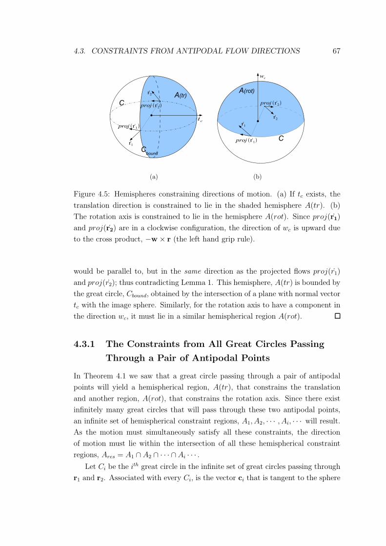
4.3. CONSTRAINTS FROM ANTIPODAL FLOW DIRECTIONS 67
(a) (b)
Figure 4.5: Hemispheres constraining directions of motion. (a) If tc exists, the
translation direction is constrained to lie in the shaded hemisphere A(tr). (b)
The rotation axis is constrained to lie in the hemisphere A(rot). Since proj(r1)
and proj(r2) are in a clockwise configuration, the direction of wc is upward due
to the cross product, −w × r (the left hand grip rule).
would be parallel to, but in the same direction as the projected flows proj(r1)
and proj(r2); thus contradicting Lemma 1. This hemisphere, A(tr) is bounded by
the great circle, Cbound, obtained by the intersection of a plane with normal vector
tc with the image sphere. Similarly, for the rotation axis to have a component in
the direction wc, it must lie in a similar hemispherical region A(rot).
4.3.1 The Constraints from All Great Circles Passing
Through a Pair of Antipodal Points
In Theorem 4.1 we saw that a great circle passing through a pair of antipodal
points will yield a hemispherical region, A(tr), that constrains the translation
and another region, A(rot), that constrains the rotation axis. Since there exist
infinitely many great circles that will pass through these two antipodal points,
an infinite set of hemispherical constraint regions, A1, A2, · · · , Ai, · · · will result.
As the motion must simultaneously satisfy all these constraints, the direction
of motion must lie within the intersection of all these hemispherical constraint
regions, Ares = A1 ∩ A2 ∩ · · · ∩ Ai · · · .
Let Ci be the ith great circle in the infinite set of great circles passing through
r1 and r2. Associated with every Ci, is the vector ci that is tangent to the sphere

68 CHAPTER 4. EGOMOTION FROM ANTIPODAL FLOW DIRECTIONS
(a) (b)
Figure 4.6: Lunes constraining directions of motion. (a) Shaded lune Ares(tr)
is the resultant constraint region on translation (b) Ares(rot) is the resultant
constraint region on rotation.
and lying in the plane of the circle Ci as defined earlier. The intersection of
constraints can then be described in Theorem 4.2 and illustrated by Figure 4.6:
Theorem 4.2. The optical flow r1 and r2 observed at any two antipodal points
r1 and r2 on the image sphere will give rise to a constraint on the translation
direction and a constraint on the rotation axis.
The translation direction lies in a region on the sphere bounded by great
circles Cbound,r1and Cbound,r2
that pass through r1 and r2 and are such that the
associated ci vectors are cbound,r1 = r1 and cbound,r2 = r2.
The direction of the rotation axis lies in a region on the sphere bounded by
great circles Cbound,r1and Cbound,r2
such that cbound,r1 is perpendicular to r1 and
cbound,r2 is perpendicular to r2.
Theorem 4.2 can be shown using a geometrical argument. For simplicity, we
consider only the vectors inhabiting the two tangent planes to the sphere at r1
and r2. They are the flow vectors and the ci vectors that are associated with
the great circles. As the two tangent planes are parallel in R3, we can represent
everything in just one plane, as is done in Figure 4.7. Every great circle passing
through a point r is characterized completely by r and ci, so in Figure 4.7, great
circles Ci and vectors ci are synonymous.
Recall that proji(r) = ci · r. So, for the case of translation, only the great cir-
cles with ci satisfying the following condition will give constraints on translation:
sgn (proj(r1)) > 0 and sgn (proj(r2)) > 0 (4.3)

4.3. CONSTRAINTS FROM ANTIPODAL FLOW DIRECTIONS 69
(a)
Figure 4.7: The two tangent planes containing r1, r2, c1 and c2 are parallel to
the plane of the page. Intersection of all hemispherical constraints on translation
is the lune Ares.
That is to say, the angles between r1 and ci and between r2 and ci must both
be less than π/2 (i.e. acute angles). Such ci vectors lie in the shaded region
U in Figure 4.7. Consider the two great circles Ca and Cb with ci’s exactly
perpendicular to r1 and r2. Let their ci vectors be ca and cb. From Theorem 4.1,
we obtain two hemispherical regions constraining translation that are bounded by
Cbound1 and Cbound2 which are again perpendicular to Ca and Cb. This means that
the ci vectors for Cbound1 and Cbound2 are actually cbound,1 = r1 and cbound,2 = r2.
The translation must lie within the intersection of these two hemispherical regions
- the region Ares of Figure 4.7.
In fact, Cbound1 and Cbound2 are the boundary cases. All other great circles
that give valid constraints on translation - those with ci’s lying between ca and
cb - will give rise to hemispherical regions that contain Ares. For example, see
the great circle represented by the vector cj in Figure 4.7. It gives rise to the
hemispherical region bounded by the great circle Cj and that hemisphere contains
Ares. So the Ares bounded by Cbound1 and Cbound2 is the smallest such region that
satisfies all the constraints. In geometry, these wedge-shaped constraint regions
are termed lunes.
To show the case of constraining rotation, simply reiterate the previous argu-
ment, but now let cbound,1 be perpendicular to r1 and cbound,2 be perpendicular to
r2.
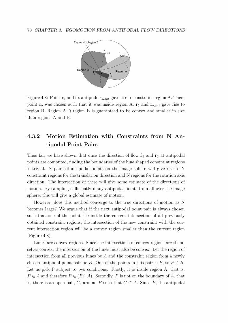
70 CHAPTER 4. EGOMOTION FROM ANTIPODAL FLOW DIRECTIONS
Figure 4.8: Point ra and its antipode ra ant gave rise to constraint region A. Then,
point rb was chosen such that it was inside region A. rb and rb ant gave rise to
region B. Region A ∩ region B is guaranteed to be convex and smaller in size
than regions A and B.
4.3.2 Motion Estimation with Constraints from N An-
tipodal Point Pairs
Thus far, we have shown that once the direction of flow r1 and r2 at antipodal
points are computed, finding the boundaries of the lune shaped constraint regions
is trivial. N pairs of antipodal points on the image sphere will give rise to N
constraint regions for the translation direction and N regions for the rotation axis
direction. The intersection of these will give some estimate of the directions of
motion. By sampling sufficiently many antipodal points from all over the image
sphere, this will give a global estimate of motion.
However, does this method converge to the true directions of motion as N
becomes large? We argue that if the next antipodal point pair is always chosen
such that one of the points lie inside the current intersection of all previously
obtained constraint regions, the intersection of the new constraint with the cur-
rent intersection region will be a convex region smaller than the current region
(Figure 4.8).
Lunes are convex regions. Since the intersections of convex regions are them-
selves convex, the intersection of the lunes must also be convex. Let the region of
intersection from all previous lunes be A and the constraint region from a newly
chosen antipodal point pair be B. One of the points in this pair is P , so P ∈ B.
Let us pick P subject to two conditions. Firstly, it is inside region A, that is,
P ∈ A and therefore P ∈ (B∩A). Secondly, P is not on the boundary of A, that
is, there is an open ball, C, around P such that C ⊂ A. Since P , the antipodal

4.4. ALGORITHM AND IMPLEMENTATION 71
point, lies on the boundary of B there exists some point Q in the neighborhood
of P such that Q ∈ A but Q /∈ B, so Q /∈ (B ∩ A). Therefore, (A ∩ B) ⊂ A, i.e.
the intersection of the original constraint region and the lune is smaller than the
original region.
Using such a scheme to choose the antipodal point pairs, as N becomes large,
the constraint region will converge to the true motion direction. Thus, for the
noise-free case of dense optical flow, we have a convergent algorithm.
In practice, we need to incorporate Hough-like voting, simulated annealing
or other such methods to account for noise, outliers and independently moving
objects that would give erroneous constraint regions. Furthermore, once the solu-
tion has been constrained to some region smaller than a hemisphere, a gnomonic
projection can map great circles on the sphere onto straight lines on a plane and
intersecting lunes onto polygons. This reduces the convex problem into a linear
one for which linear programming methods are a possible solution.
Once the translation and rotation axis have been recovered, estimating the
magnitude of rotation is easy and several methods are possible. Here is one
suggestion: r = ftr(r) + frot(r) (Equation 4.1) is a vector sum triangle. We now
know the directions of ftr(r) and frot(r), that is, we know the angles between the
sides of that triangle. Thus, magnitude of frot(r) can be found by the sine rule of
triangles. Repeating for several points on the image, an overconstrained system
of linear equations is obtained and a least squares solution to rotation angle may
be found.
4.4 Algorithm and Implementation
The quickly converging method earlier described could be used if speed was crit-
ical, but here, we use a simple but robust vote-based algorithm summarized in
Algorithm 4.1. The steps for estimating translation and for finding the rotation
axis are similar.
Our implementation uses coarse-to-fine voting. First, we pick the flow at
Mcoarse pairs of antipodes and obtain Mcoarse constraints as detailed in Theorem
4.2. Having divided the image sphere into a two-dimensional voting table ac-
cording to the azimuth-elevation convention, we proceed to vote in each lune or
constraint region obtained. This is the coarse voting stage and the area on the
sphere represented by a voting bin can be fairly large. The bin with maximum
votes is then found, giving us a coarse estimate of either the translation or the

72 CHAPTER 4. EGOMOTION FROM ANTIPODAL FLOW DIRECTIONS
Algorithm 4.1 Estimating the translation (or rotation axis) by voting
1: for i = 1 to Mcoarse do
2: Select a pair of antipodes r1, r2 with optical flow r1, r2.
3: Obtain the constraint region on translation (or rotation axis) and the great
circles bounding the lune as per Theorem 4.2.
4: The spherical coordinates (θ, φ) of points on the lune is calculated and
coarse voting is performed.
5: end for
6: Find the bin(s) with maximum votes. This gives the coarse estimate.
7: Choose a projection plane at or close to the coarse estimate.
8: for j = 1 to Mfine do
9: Repeat steps 2 to 3 to obtain the lune and its bounding great circles.
10: Project the lune onto the projection plane. This maps the bounding great
circles onto straight lines.
11: Vote on the projected lune on the plane.
12: end for
13: Find the bin(s) with maximum votes. This gives the fine estimate.
rotation axis. If more than one bin has maximum votes, the average direction is
used instead. An example of the result of coarse voting on the sphere is shown
in Figure 4.9.
0 20 40 60 80 100050100150200
0
50
100
150
200
250
300
350
400
450
500
phi
Azimuth (theta) and elevation (phi) vs votes
theta
vote
s
Figure 4.9: Voting on the sphere.
For the fine voting stage, a region of the image sphere in the neighborhood
of the coarse estimate is projected onto a plane that is tangent to a point on the
sphere (refer Figure 4.10). The point can be at the location of the coarse estimate
found earlier or anywhere near it. The center of projection is the sphere center

4.4. ALGORITHM AND IMPLEMENTATION 73
and the mapping will project points on the surface of the sphere onto the tangent
plane. Let the sphere centre be the origin and rsph be a point that lies on the unit
image sphere. If the plane is tangent to the sphere at a point n, then n is also a
unit normal of that plane. In that case, the projection of rsph onto the plane is a
point, rpln, that lies on the tangent plane and is given by rpln = rsph/(rsph · n).
Figure 4.10: Projection of a point rsph which lies on the image sphere, to a point
rpln which lies on the plane that is tangent to the sphere at point n. tcoarse is
the coarse estimate of translation found after the coarse voting stage (the same
applies for estimating rotation axis).
This is called a gnomonic projection [44]. This projection will map great circles
on the sphere onto straight lines on the plane1. The motivation for performing
the fine voting stage on a projection plane rather than on the image sphere is the
greater efficiency and simplicity in voting on the plane.
After each voting stage, the centre of mass of the bin(s) with the highest
votes gives the Maximum Likelihood estimate of motion direction. If necessary,
the planar voting stage can be repeated for progressively finer scales such as with
the schemes proposed by [11, 109]. We chose a vote-based approach because it is
highly robust to noise and outliers in the flow. Its disadvantage is that accuracy
is limited by voting bin resolution.
Other variations on voting are also possible. For example, many optical flow
calculation methods return a covariance matrix which gives an uncertainty mea-
sure of the accuracy of the calculated flow. Hence, lunes resulting from flow
with high accuracy can be given higher weights during voting compared to lunes
1Note: A stereographic projection is subtly different from the gnomonic projection. The
centre of projection for the former may lie anywhere on the surface of the sphere, whilst the
projection centre for the latter is the sphere centre.

74 CHAPTER 4. EGOMOTION FROM ANTIPODAL FLOW DIRECTIONS
arising from less accurate flow. In our experiments however, we found that the
unmodified version of the algorithm was sufficiently robust and accurate and we
did not require any such extra measures.
4.5 Discussion and Summary
In summary, our method directly recovers both the translation and rotation axis
using two sets of constraints. These constraints on translation and rotation are
geometrically dual to each other. Both the translation and rotation axis can
be recovered in parallel since they can be estimated separately from each other.
Once these directions of motion are known, the magnitude of rotation may also
be recovered.
Features of the voting algorithm: The algorithm we presented is a ‘non-
numerical’ approach - that is, the constraints are obtained without numerically
solving equations. In fact, no mathematical operations more complex than that
required for voting will be performed. Furthermore, run-time is constant with
increasing noise and outliers (see experiments in Chapter 6), and that, together
with the naturally parallelizable nature of voting makes it potentially viable for
implementation as a real-time egomotion recovery system.
Directions of flow: An interesting concept in this approach was the use of
only the directions of flow vectors, and not their magnitudes. This leads to
weaker, lune-shaped constraints. However, by using only directions of flow, we
are able to extend antipodal constraints to rotation as well (in the next chapter,
we derive constraints using both the directions and magnitudes of antipodal flow,
but that only constrains translation direction). Other benefits include improved
robustness since it is independent of noise in the magnitude of flow vectors - only
noise in the direction of flow affects it. It is also theoretically interesting because
our constraint regions (the lunes) arise immediately from the flow vectors without
further mathematical processing, be it addition, multiplication or more complex
operations.
Fail-soft. Insufficient antipodal points does not break the algorithm - the
motion only becomes more ambiguous. The vote-table is a probability map,
where regions of higher votes indicate higher probability of the motion being in
that direction. Ambiguity occurs when constraints fail to further disambiguate
motion, and a patch of directions has tied votes. The true solution lies within
that patch with maximum probability given the available antipodes. This is

4.5. DISCUSSION AND SUMMARY 75
better than many other motion methods that return a nonsensical number when
they fail.

Chapter 5
Translation from Flow at
Antipodal Points
In the last chapter, we presented constraints on both the translation direction
as well as the axis of rotation using purely directions of antipodal flow. In this
chapter, we consider a different approach which uses the magnitude of the antipo-
dal flow vectors as well. Once again, recall that we are dealing with differential
camera egomotion (discrete camera motions are considered in Part III).
In brief, we will use the optical flow at two antipodal points to constrain the
translation direction to lie on a great circle (that is, the intersection of a plane
through the camera center with the image sphere). The rotational contribution
to the measured optical flow is eliminated, leaving an equation dependent only on
the translational component of motion. Multiple such constraints are then used
to estimate the translation uniquely (up to a scale, of course).
Compared to the approach in the last chapter, we obtain much stronger con-
straints on the direction of translation (we constrain it to a great circle, instead of
a lune). This happens because we use all the information from the antipodal flow
- i.e. both the magnitudes as well as the directions. However, the downside is that
no constraints on rotation arise directly since we effectively cancel the rotational
effects with our method. Even so, we will show that once translation has been
found, a least squares estimate of rotation that is robust to outliers would not be
difficult to recover.
We note that Thomas and Simoncelli [233] observed an antipodal point con-
straint that is related to the constraint presented in this chapter. However, signif-
icant differences in the theoretical derivation and in the resulting constraint exist
between the method of [233], and our work (see Section 5.1.1). Our constraint
77

78 CHAPTER 5. TRANSLATION FROM FLOW AT ANTIPODAL POINTS
is somewhat simpler to derive and use compared to [233] and it succeeds in cer-
tain scene depth configurations where theirs fails. Both the constraint presented
here and that of [233] may be thought of as special cases of the linear subspace
methods investigated by Jepson and Heeger [114].
5.1 Removing Rotation by Summing Flow at
Antipodal Points
Once again, we consider the optical flow, r1, at some point, r1, on an image
sphere:
r1 =1
| R(r1) |((t · r1)r1 − t) − w × r1 (5.1)
Suppose there is another point, r2, that is antipodal to r1, that is, r2 = −r1.
Then the optical flow at the second point is:
r2 =1
| R(r2) |((t · r2)r2 − t) − w × r2
=1
| R(−r1) |((t · r1)r1 − t) + w × r1
(5.2)
By summing Equations 5.1 and 5.2, we have an expression that arises purely from
the translational component of motion. The rotational components cancel out.
rs = r1 + r2
= (1
| R(r1) |+
1
| R(−r1) |)((t · r1)r1 − t)
= A((t · r1)r1 − t)
(5.3)
From Equation 5.3, we see that vectors r1, rs and t are coplanar. The normal
of that plane is given by r1 × rs where × denotes the vector cross product. The
direction of translation, t, lies on that plane. The intersection of that plane with
the image sphere gives a great circle. See Figure 5.1(a) for an illustration.
By picking another pair of antipodal points (that do not lie on the first great
circle) and repeating, we obtain a second such plane or great circle. The inter-
section of the two planes or great circles gives an estimate of translation, t. See
Figure 5.1(b) for an illustration.

5.1. REMOVING ROTATION BY SUMMING FLOW 79
(a) (b)
Figure 5.1: (a) Summing the flow r1 and r2 yields the vector rs, which, together
with r1 (or r2), gives rise to a plane on which t is constrained to lie. The
intersection of that plane with the sphere is the great circle C. (b) From two
pairs of antipodal points, two great circles C1 and C2 are obtained. t is the
intersection of these two circles.
Of course, the intersection of the two great circles actually yields two points
corresponding to t and −t. To disambiguate between the two, one may pick one
of the two points and calculate the angle between it and the vector rs. If the
angle is larger than π/2 radians, then that point is t. Otherwise, it is −t.
5.1.1 Comparison with Thomas and Simoncelli
The underlying principle here was first observed in Thomas and Simoncelli [233].
However, major differences differentiate this work from that of [233]. The ap-
proach used there defined angular flow, which is obtained by taking the cross
product of optical flow at a point with the direction of that point. In effect, a
dual representation of flow is obtained and [233] showed that if the angular flow
at two antipodal points was subtracted from each other, the rotational component
would vanish.
Both the constraint developed here and the one in [233] probably stem from
a similar geometrical property inherent to antipodal points but the methods by
which they were derived and the final results are quite different. The constraint
in this paper does not require the transformation of optical flow into angular flow
as in [233], a step which incurs an additional cross product.
80 CHAPTER 5. TRANSLATION FROM FLOW AT ANTIPODAL POINTS
Furthermore, the method of [233] requires a subtraction of angular flow at
antipodal points and thus, that method fails when the world points projecting
onto the antipodal points on the imaging device are at equal distances from
the camera centre (subtracting the angular flow in that case yields zero) - a
problem observed by the authors of that paper. An example of this would be the
distances to the two opposite walls when the camera is exactly in the middle of a
corridor (note that this is an important and commonly occurring scenario in many
autonomously navigating systems, for example, the corridor centring behaviour
of honeybees and robots [217, 216, 218]). The method presented in this paper
sums the optical flow at antipodal points and therefore, does not encounter such
instabilities when antipodal scene points are at equal, or close to being at equal
distances.
Finally, because omnidirectional and panoramic sensors were not widely avail-
able then, the method of [233] was not fully developed into an algorithm and no
implementations or experiments were ever conducted. Here two complete algo-
rithms are presented, tested on simulations under increasing noise and outliers,
and demonstrated to work on fairly difficult real image sequences.
Closely related, is the more recent work of Hu and Cheong [106], which de-
velops a constraint similar to that of [233], where the optical flow at antipodal
points is subtracted to yield a constraint on translation1. As a result, [106] is also
degenerate when the world points corresponding to the antipodal rays used are
at near-equal distances from the camera centre.
5.2 Obtaining robust estimates of translation
We now have a method for obtaining some estimate of the direction of t given
the flow at any pair of antipodal points. In this section, we outline methods for
doing this robustly. Two classes of approaches are possible and we present an
algorithm representative of each class in Sections 5.2.1 and 5.2.2.
Class 1: Point-Based - Firstly, the flow at two pairs of antipodal points gives
a unique (up to a scale) solution for the translation from the intersection of two
great circles. Repeatedly picking 2 pairs from a set of N antipodal point pairs
1In [106], the authors work with what they term ‘matching rays’, which come from two
laterally mounted cameras pointing in opposite directions such that their FOVs do not overlap
(a setup reminiscent of the laterally directed eyes of many birds or fish). However, they then
assume that the separation between the two cameras is small, which effectively reduces these
‘matching rays’ to antipodal points.

5.2. OBTAINING ROBUST ESTIMATES OF TRANSLATION 81
can give up to NC2 = N !2!(N−2)!
possible solutions, where each candidate solution is
a point on the image sphere. We loosely term the class of methods that estimates
the best solution from a set of point solutions, point-based algorithms.
Section 5.2.1 presents an algorithm representative of this class that finds the
solution point best supported by the optical flow data using the RANSAC frame-
work. Moreover, since the points all lie in a Lie-group (which a sphere is), Tuzel
et al. [249] showed that the mean shift algorithm [43] may also be used for finding
the mode of the points. K-means is another possibility for clustering points on
a sphere [238]. Other algorithms in this class include robust estimators such as
[37], and variants of RANSAC such as [241, 155, 156, 180].
Class 2: Line/Curve-Based - Alternatively, since the flow at every pair of
antipodes yields a great circle which must intersect t, the translation could be
estimated by simultaneously finding the best intersection of many of these great
circles. We will later show this can be reduced to the problem of intersecting
straight lines. Once again, many algorithms exist, including linear and convex
programming. We observe that the problem is quite similar to that of intersecting
many vanishing lines to find the vanishing point [196, 151, 210], and inspired by
a popular solution in this area, we use a Hough-reminiscent voting approach.
There are of course myriad variations to Hough voting (such as [104, 54, 110,
11, 271, 109]) and we present an algorithm representative of the class which is
not necessarily the best solution, but which nevertheless works very well in the
experiments.
Algorithms that are a combination of the two classes are also possible, such
as finding the best supported solution with RANSAC, and then doing linear
programming using the inlier flow measurements that have been found.
5.2.1 RANSAC
Algorithm 5.1 summarizes our use of the constraint within the RANSAC sam-
pling algorithm. M is the number of iterations of the algorithm and is calculated
adaptively as:
M =log(1 − p)
log(1 − ws)(5.4)
where p is the probability of choosing at least one sample of data points free of
outliers, w is the inlier probability, and s is the number of data points required
to obtain a candidate solution.

82 CHAPTER 5. TRANSLATION FROM FLOW AT ANTIPODAL POINTS
Algorithm 5.1 Estimating translation direction - RANSAC algorithm1: Set M = ∞, count = 0
2: while M > count AND count < MAX do
3: Select a pair of antipodes r1, r2 with optical flow r1, r2.
4: rs = r1 + r2 and n1 = rs × r1
5: Repeat for a different pair of antipodes to obtain n2 such that n1 6= n2
6: Take cross product t = n1 × n2
7: for i = 1 to N do
8: For the ith antipodal pair, find the plane normal ni
9: If π2− cos−1(ni · t) < θthres, increment support for t
10: end for
11: Update M , increment count
12: end while
13: The best supported t is the solution.
N is the number of antipodal flow measurements available. MAX is the
upper limit on number of iterations to guarantee termination of the algorithm.
If several solutions have the same maximum support, then some mean of their
directions can be used instead. Details of the RANSAC framework may be found
in Section 3.1.5, page 47.
In this algorithm, lines 3 to 6 randomly pick antipodal points and generate
hypothesis solutions from the intersection of two planes as discussed earlier. In
lines 8 and 9, the candidate solution t is then scored according to the number
of antipodal flow data vectors that support it. An antipodal flow pair supports
the candidate translation if the angle between the translation vector and the
constraint plane generated by that flow pair is less than some threshold angle,
θthres. The candidate with the most support from the flow data is the estimated
translation.
The method is quite simple but very robust, as the results in Chapter 6
will show. However, some tuning of the parameters is required for best results.
Furthermore, as with all RANSAC-type algorithms, the processing time increases
with the probability of outliers and noise in the data. If speed is critical, then a
more efficient method may be necessary, which leads us to the voting approach
in the next section.

5.2. OBTAINING ROBUST ESTIMATES OF TRANSLATION 83
Algorithm 5.2 Estimating translation direction - voting algorithm
1: for i = 1 to Mcoarse do
2: Select a pair of antipodes r1, r2 with optical flow r1, r2.
3: rs = r1 + r2
4: The sphere center, vectors rs and r1 (or its antipode, r2) define a great
circle, Ci on the image sphere.
5: The spherical coordinates (θ, φ) of points on great circle Ci are calculated
and coarse voting is performed.
6: end for
7: Find the bin with maximum votes. This is the coarse estimate.
8: Choose a projection plane at or close to coarse estimate.
9: for j = 1 to Mfine do
10: Repeat steps 2 to 4 to obtain a great circle Cj.
11: Project Cj onto the projection plane to obtain a straight line Lj .
12: Perform fine voting by voting along the straight line Lj .
13: end for
14: Find the bin with maximum votes. This is the fine estimate.
5.2.2 Hough-reminiscent Voting
Another approach that we identified for robustly estimating translation direction,
t, was to simultaneously find the best intersection of all the great circles arising
from our method of summing flow at antipodal points. An efficient way of doing
this is via a Hough-reminiscent voting method as summarized in Algorithm 5.2.
The procedure follows closely the algorithm described in Chapter 4, however, here
we vote on great circle constraints, instead of the lune constraint regions of the
last chapter.
In the coarse voting stage, we pick the flow at Mcoarse pairs of antipodes and
obtain Mcoarse great circles with the steps detailed in Section 5.1. We vote on
these great circles and find the peak in the vote table to obtain the coarse estimate
of translation, tcoarse.
Once again, we project a region on the image sphere in the neighborhood of the
coarse estimate onto a plane via the gnomonic projection and perform our voting
on the projections of great circles - i.e. on straight lines on that plane. This is
an advantageous mapping since very efficient algorithms for voting along straight
lines exist, such as the Bresenham line algorithm [27]. Once again, voting may
be repeated for finer scales if necessary. An example of the result of fine voting
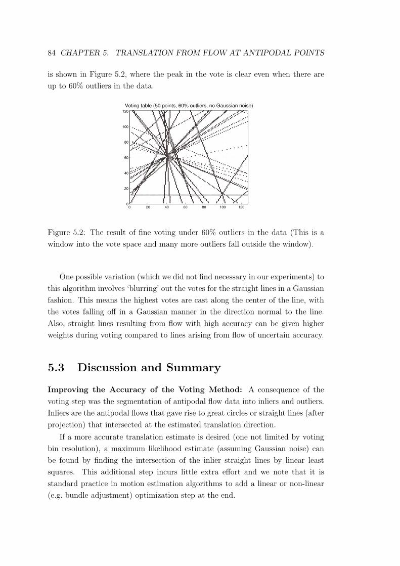
84 CHAPTER 5. TRANSLATION FROM FLOW AT ANTIPODAL POINTS
is shown in Figure 5.2, where the peak in the vote is clear even when there are
up to 60% outliers in the data.
0 20 40 60 80 100 1200
20
40
60
80
100
120
Voting table (50 points, 60% outliers, no Gaussian noise)
Figure 5.2: The result of fine voting under 60% outliers in the data (This is a
window into the vote space and many more outliers fall outside the window).
One possible variation (which we did not find necessary in our experiments) to
this algorithm involves ‘blurring’ out the votes for the straight lines in a Gaussian
fashion. This means the highest votes are cast along the center of the line, with
the votes falling off in a Gaussian manner in the direction normal to the line.
Also, straight lines resulting from flow with high accuracy can be given higher
weights during voting compared to lines arising from flow of uncertain accuracy.
5.3 Discussion and Summary
Improving the Accuracy of the Voting Method: A consequence of the
voting step was the segmentation of antipodal flow data into inliers and outliers.
Inliers are the antipodal flows that gave rise to great circles or straight lines (after
projection) that intersected at the estimated translation direction.
If a more accurate translation estimate is desired (one not limited by voting
bin resolution), a maximum likelihood estimate (assuming Gaussian noise) can
be found by finding the intersection of the inlier straight lines by linear least
squares. This additional step incurs little extra effort and we note that it is
standard practice in motion estimation algorithms to add a linear or non-linear
(e.g. bundle adjustment) optimization step at the end.

5.3. DISCUSSION AND SUMMARY 85
Finding Rotation Robustly: We remind the reader that at this point, we
have only recovered the direction of translation. The rotation was not estimated
directly from our method. However, knowing translation, it becomes much easier
to then estimate rotation. For instance, taking dot products on both sides of
Equation 5.1 with t× r eliminates dependence on depth:
(t × r) · r = (t × r) · (1
| R(r) |((t · r)r− t)) − (t × r) · (w × r)
(t × r) · r = (t × r) · (w × r)
(5.5)
The estimated translation direction is substituted into Equation 5.5, giving
us an equation linear in rotation, w. Taking flow at several points, we can build
a system of over-constrained linear equations which is solvable by the method
of linear least squares. This would be done using only the inlier flow vectors
obtained from the translation estimation stage, so the rotation estimate would
also be independent of outliers. However, whilst almost all outlier flow vectors
were discarded, it is still possible for a few outliers to slip in (called ‘leverage
points’ in statistics). This happens if, by chance, the noise in two outlier antipo-
dal flow vectors cancel when added, giving a great circle that passes through the
translation direction. Therefore, another layer of outlier rejection may be needed
in practice. Fortunately, since previous steps would have reduced the number of
unknowns and weeded out almost all outliers, this should converge very quickly.
In summary, we have presented a simple but effective constraint on the trans-
lation direction from antipodal points. The constraint restricts the translation to
lie on a plane (or great circle on the image sphere) and is a stronger constraint
compared to the one introduced in Chapter 4. However, rotation then needs to
be found via a second step, by substituting the translation back into the motion
equations. Also, errors in the translation estimate may propagate forward to the
rotation estimate. Hence, one solution may be to use the stronger great circle
constraints to estimate translation, and to use the lune constraints of Chapter 4
to recover rotation.


Chapter 6
Experiments and Comparison of
Results
In the last two chapters, we presented two different antipodal point-based con-
straints for egomotion recovery. The constraint of Chapter 4 used the directions
of antipodal flow vectors to constrain the directions of egomotion. Meanwhile,
in Chapter 5, we summed the flow at antipodal points to obtain constraints on
translation. We also introduced a robust Hough-like voting algorithm that uti-
lized the first constraint, whilst another two algorithms (based on Hough-voting
and on RANSAC) utilized the second constraint.
In this chapter, we demonstrate that the constraints presented in Chapters
4 and 5 work, and that the usage of antipodal points is practical for egomotion
recovery. The algorithms based on our two constraints are tested in experiments
using real images, as well as in simulations under noise and outliers. The results in
the following sections will show that algorithms based on our antipodal point con-
straints performed competitively with the state-of-the-art whilst demonstrating
advantages in their robustness to large outlier proportions and in the processing
time required.
Comparison between our two approaches: The Hough-like voting algo-
rithm of Chapter 4 is referred to as the “Lune+voting” method since it votes
on lune-shaped constraint regions. Meanwhile, the RANSAC-based and voting-
based algorithms of Chapter 5 are referred to as “GC+RANSAC” and “GC+voting”
methods respectively (the “GC-” prefix refers to the great circle regions arising
from the intersection of the planar constraints with the image sphere).
Lune+voting is used to recover the camera translation direction and rotation
axis. Meanwhile, GC+RANSAC and GC+voting only directly recover transla-
87

88 CHAPTER 6. EXPERIMENTS AND COMPARISON OF RESULTS
tion1. The angle between the estimated motion direction and the true motion
(known in simulations, and measured in real experiments) then gives the error in
the estimates.
Comparison against the state-of-the-art: Since we are working with cal-
ibrated cameras, we compare the performance of our methods against the 5-point
algorithm of Li and Hartley [136] within a robustifying RANSAC framework2.
We will refer to this as the “5-point+RANSAC” method.
We chose 5-point+RANSAC as a comparison since it is well-known, well-
studied, widely used and code is widely available. Code for the five-point algo-
rithm was made available by the authors of [136]. This five-point minimal solver
worked within a RANSAC framework using code from [127]. Sampling was adap-
tive and the probability with which a good solution was to be found was set to
p = 0.99. As discussed in page 47 (refer also [93]), the method attempts to esti-
mate the proportion of outliers in the data and adaptively adjusts the number of
samples used. The quality of hypothesis solutions was measured as the Sampson
distance approximation of reprojection error, which was set at a threshold of 0.01.
6.1 Simulations
6.1.1 Experimental Method
We simulated the camera to simultaneously rotate and translate such that an
optical flow field was generated. Since the imaging surface is a sphere and flow
is available in every direction, we can fix the direction of translation without any
loss of generality as the result would be the same in any direction. The axis of
rotation however, was varied randomly from trial to trial since the angle made
between the direction of translation and axis of rotation does in fact influence the
outcome. Baseline was 2 units and the rotation angle 0.2 radians. 500 pairs of
1As discussed before, with known translation, the rotation can be easily recovered in a second
step. However, we will not focus on that here as our emphasis is on testing and validating the
antipodal constraints.2Although the 5-point algorithm is considered to be a discrete-motion method, it works quite
well for a large range of motion sizes, including fairly small motions. Various other discrete-
motion methods have also been found to work well for small motions (refer Section 3.1.1, page
34), and the 5-point algorithm has previously been used as a benchmark in papers on differential
motion methods (e.g. Stewenius et al. [221]). For the motion sizes used in our experiments, we
found 5-point to work reasonably well with sub-pixel accuracy for zero noise and < 1◦ error for
small noise (Figures 6.1, 6.2 and 6.3).

6.1. SIMULATIONS 89
random antipodal scene points were uniformly distributed in all directions with
depth ranging from 10 to 15 units. Results were averaged over 100 trials.
In the simulations, 5-point used the point matches as input whilst our method
took the flow vectors as input. Experiments were conducted for increasing prob-
ability of outliers (with no Gaussian noise) and also for an increasing level of
Gaussian noise (with no added outliers). Outliers were simulated by randomly
replacing matches or flow with errors. To simulate Gaussian noise, the position
of a matched point was perturbed from its true value by a noise vector modeled
as a 2D Gaussian distribution with standard deviation σ and zero mean.
6.1.2 Robustness to Outliers
0 0.1 0.2 0.3 0.4 0.50
0.5
1
1.5
2
2.5
3
3.5
4
4.5
5
Outlier Proportion
Err
or
(deg)
Translation Error vs Outliers
5pt+RANSAC
GC+voting
GC+RANSAC
(a)
0 20 40 60 80 100 1200
20
40
60
80
100
120
Voting table (50 points, 60% outliers, no Gaussian noise)
(b)
Figure 6.1: (a) Error in estimated translation as proportion of outliers in data
increases. The benchmark method - 5-point+RANSAC - is also shown. Com-
parison between the two great-circle (GC) constraint based algorithms. (b) The
result of the fine voting stage of GC+voting.
GC+RANSAC versus GC+voting: The errors for the two algorithms that
summed antipodal flow to obtain great-circle constraints on translation are shown
in Figure 6.1(a). As the figure demonstrates, all methods performed robustly
under increasing outlier proportions. GC+RANSAC and GC+voting showed
no appreciable increase in error even for outlier proportions of as high as 50%.
In contrast, errors for 5-point+RANSAC increased visibly by up to 5◦ as the
proportion of outliers grew. Note that the errors for GC+voting were slightly
higher than GC+RANSAC due to quantization error during voting (which may
be further mitigated by using finer scales, and performing linear or nonlinear
refinement on these results).
Here, errors in 5-point+RANSAC arise because some outliers fall within the

90 CHAPTER 6. EXPERIMENTS AND COMPARISON OF RESULTS
model distance threshold used (0.01). Reducing the RANSAC distance thresh-
old improves performance; but in general, both our antipodal methods tended
to outperform 5-point+RANSAC for very large outlier proportions. This is an
interesting result and there are several reasons for it, as discussed in the following.
The Hough-like voting algorithm is extremely resistant to outliers. Figure
6.1(b) shows the votes cast in a voting table for 60% random outliers in the data.
The figure shows the straight lines obtained from projecting great circles onto a
plane during the fine-voting stage of the GC+voting algorithm. Inlier straight
lines intersect at a common point whilst the outlier straight lines do not. Most
of them fall outside the region of the plane shown in the figure but quite a few
outliers can still be seen. From the figure, it is clear that the intersection can
easily be found even for this high proportion of outliers.
The GC+RANSAC framework worked better because it needed only 2 points
for a constraint as opposed to 5 points for the 5-point+RANSAC algorithm. If q
is the probability of an inlier, then the probability of obtaining a good constraint
is q2 for the antipodal method and q5 for 5-point. Therefore, both antipodal
methods are always more likely to obtain more good constraints when flow at
antipodal points is available.
Performance of Lune+voting: Figure 6.2(a) compares the results of lune+voting
with that of 5-point+RANSAC and of GC+voting (GC+RANSAC gives very sim-
ilar results, which we do not show). Unsurprisingly, 5-point+RANSAC estimates
translation most accurately for low noise since voting bin resolution limits our
methods in this implementation. Interestingly, both lune+voting and GC+voting
outperformed 5-point+RANSAC as outliers grew. Compared to GC+voting, the
lune+voting method has higher error, since it uses a weaker constraint.
0 0.1 0.2 0.3 0.40
1
2
3
4
5
Outlier Proportion
Err
or
(de
g)
Translation error vs Outliers
lune+voting
5pt+RANSAC
GC+voting
(a)
0 0.1 0.2 0.3 0.4 0.50
1
2
3
4
5
Outlier Proportion
Err
or
(de
g)
Rotation axis error vs Outliers
lune+voting
5pt+RANSAC
(b)
Figure 6.2: Error in estimated motion as proportion of outliers in data increases.
(a) Performance of lune+voting method for translation and (b) for rotation.
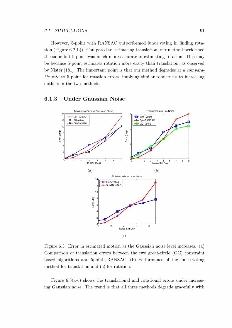
6.1. SIMULATIONS 91
However, 5-point with RANSAC outperformed lune+voting in finding rota-
tion (Figure 6.2(b)). Compared to estimating translation, our method performed
the same but 5-point was much more accurate in estimating rotation. This may
be because 5-point estimates rotation more easily than translation, as observed
by Nister [181]. The important point is that our method degrades at a compara-
ble rate to 5-point for rotation errors, implying similar robustness to increasing
outliers in the two methods.
6.1.3 Under Gaussian Noise
0 1 2 3 4 5 6 70
2
4
6
8
10
12
14
Std Dev (deg)
Err
or
(deg)
Translation Error vs Gaussian Noise
5pt+RANSAC
GC+voting
GC+RANSAC
(a)
0 1 2 3 4 5 6 7 8 90
5
10
15
Noise Std Dev
Err
or
(deg)
Translation error vs Noise
lune+voting
5pt+RANSAC
GC+voting
(b)
0 2 4 6 80
2
4
6
8
10
12
14
Noise Std Dev
Err
or
(deg)
Rotation axis error vs Noise
lune+voting
5pt+RANSAC
(c)
Figure 6.3: Error in estimated motion as the Gaussian noise level increases. (a)
Comparison of translation errors between the two great-circle (GC) constraint
based algorithms and 5point+RANSAC. (b) Performance of the lune+voting
method for translation and (c) for rotation.
Figure 6.3(a-c) shows the translational and rotational errors under increas-
ing Gaussian noise. The trend is that all three methods degrade gracefully with

92 CHAPTER 6. EXPERIMENTS AND COMPARISON OF RESULTS
increasing noise. However, for large Gaussian noise, our antipodal point meth-
ods tended to perform better than 5-point+RANSAC since some of the noisy
data points were falling within the set threshold (for distinguishing inliers from
outliers) of the RANSAC framework.
6.1.4 Processing time
0 0.1 0.2 0.3 0.4 0.50
20
40
60
80
100
120
140
160
180
200
Outlier Proportion
Tim
e (
sec)
Run time vs Outliers
5pt+RANSAC
GC+voting
lune+voting
Figure 6.4: Run time versus increasing outlier proportions (Matlab implementa-
tions running on an Intel Pentium Dual Core CPU 3GHz, 1GB RAM).
We have seen that our vote-based antipodal algorithms (GC+voting and
lune+voting) show comparable robustness with 5-point and RANSAC. Figure
6.4 further demonstrates that our algorithms achieve this with constant pro-
cessing time under increasing proportions of outliers. Conversely, run-time for
RANSAC increases quickly as the outlier proportion increases (in the exper-
iment of Figure 6.4, the increase is approximately cubic). Our algorithm is
constant time because voting is efficient and fast enough to use all available
flow, whereas 5-point+RANSAC samples points adaptively according to N =
log(1 − p)/log(1 − (1 − ǫ)s) (see page 47). The numbers in Figure 6.4 are obvi-
ously implementation dependent but the trend will remain the same.
Note also that the processing time of RANSAC is dependent on the distance
threshold used for distinguishing inliers from outliers. The Sampson distance
threshold used was 0.01; if a stricter threshold was used, 5-point+RANSAC would
perform better in the outlier and Gaussian noise experiments, however, its pro-
cessing time performance would then worsen correspondingly. Our methods do
not trade-off accuracy for run-time.
Compared to GC+voting, the lune+voting algorithm obviously takes more
time, since the constraint regions it needs to vote over are larger (lunes versus
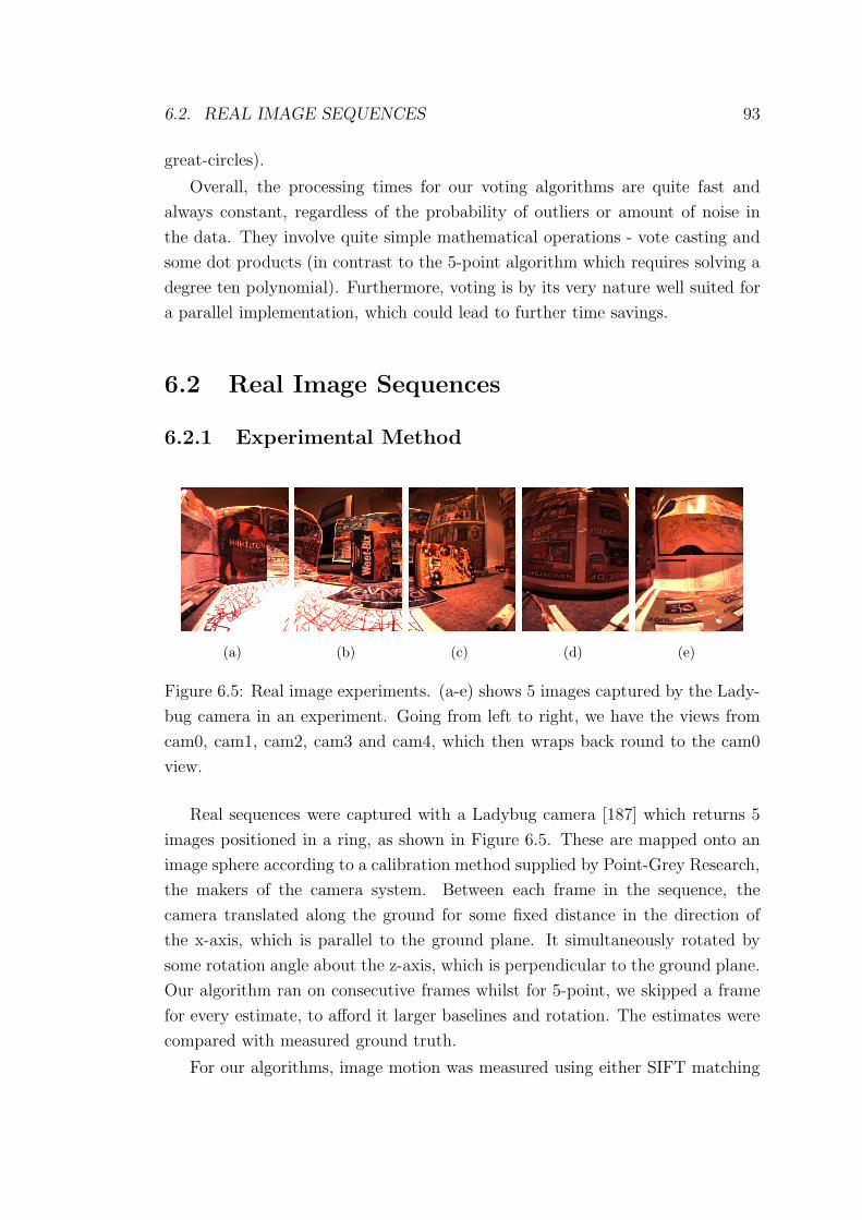
6.2. REAL IMAGE SEQUENCES 93
great-circles).
Overall, the processing times for our voting algorithms are quite fast and
always constant, regardless of the probability of outliers or amount of noise in
the data. They involve quite simple mathematical operations - vote casting and
some dot products (in contrast to the 5-point algorithm which requires solving a
degree ten polynomial). Furthermore, voting is by its very nature well suited for
a parallel implementation, which could lead to further time savings.
6.2 Real Image Sequences
6.2.1 Experimental Method
(a) (b) (c) (d) (e)
Figure 6.5: Real image experiments. (a-e) shows 5 images captured by the Lady-
bug camera in an experiment. Going from left to right, we have the views from
cam0, cam1, cam2, cam3 and cam4, which then wraps back round to the cam0
view.
Real sequences were captured with a Ladybug camera [187] which returns 5
images positioned in a ring, as shown in Figure 6.5. These are mapped onto an
image sphere according to a calibration method supplied by Point-Grey Research,
the makers of the camera system. Between each frame in the sequence, the
camera translated along the ground for some fixed distance in the direction of
the x-axis, which is parallel to the ground plane. It simultaneously rotated by
some rotation angle about the z-axis, which is perpendicular to the ground plane.
Our algorithm ran on consecutive frames whilst for 5-point, we skipped a frame
for every estimate, to afford it larger baselines and rotation. The estimates were
compared with measured ground truth.
For our algorithms, image motion was measured using either SIFT matching
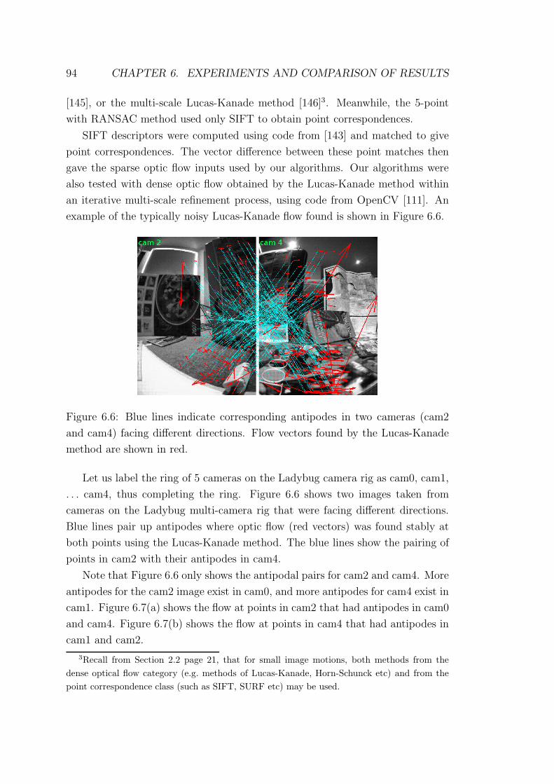
94 CHAPTER 6. EXPERIMENTS AND COMPARISON OF RESULTS
[145], or the multi-scale Lucas-Kanade method [146]3. Meanwhile, the 5-point
with RANSAC method used only SIFT to obtain point correspondences.
SIFT descriptors were computed using code from [143] and matched to give
point correspondences. The vector difference between these point matches then
gave the sparse optic flow inputs used by our algorithms. Our algorithms were
also tested with dense optic flow obtained by the Lucas-Kanade method within
an iterative multi-scale refinement process, using code from OpenCV [111]. An
example of the typically noisy Lucas-Kanade flow found is shown in Figure 6.6.
Figure 6.6: Blue lines indicate corresponding antipodes in two cameras (cam2
and cam4) facing different directions. Flow vectors found by the Lucas-Kanade
method are shown in red.
Let us label the ring of 5 cameras on the Ladybug camera rig as cam0, cam1,
. . . cam4, thus completing the ring. Figure 6.6 shows two images taken from
cameras on the Ladybug multi-camera rig that were facing different directions.
Blue lines pair up antipodes where optic flow (red vectors) was found stably at
both points using the Lucas-Kanade method. The blue lines show the pairing of
points in cam2 with their antipodes in cam4.
Note that Figure 6.6 only shows the antipodal pairs for cam2 and cam4. More
antipodes for the cam2 image exist in cam0, and more antipodes for cam4 exist in
cam1. Figure 6.7(a) shows the flow at points in cam2 that had antipodes in cam0
and cam4. Figure 6.7(b) shows the flow at points in cam4 that had antipodes in
cam1 and cam2.
3Recall from Section 2.2 page 21, that for small image motions, both methods from the
dense optical flow category (e.g. methods of Lucas-Kanade, Horn-Schunck etc) and from the
point correspondence class (such as SIFT, SURF etc) may be used.

6.2. REAL IMAGE SEQUENCES 95
(a) (b)
Figure 6.7: (a) All the antipodal flow that was found for the cam2 image using
views from cam0 and cam4. (b) All antipodal flow found for the cam4 image
using views from cam1 and cam2.
The Lucas-Kanade method computed flow at fixed positions in a grid, so that
the antipodal points were already user defined. Flow vectors with large error
(the flow algorithm returns an uncertainty measure) were thrown away, but a
few obvious mismatches remain. However, most of the flow appears reasonably
stable. Over the entire view-sphere, for these experiments, flow was found for
about 500 - 700 pairs of antipodes, which is generally more than our algorithms
need for a good estimate.
The SIFT algorithm computes SIFT points at particular positions in the image
that the algorithm deems likely to be robust to changes in scale [145]. Therefore,
to find antipodal points, one has to perform an exhaustive search over all SIFT
matches returned by the algorithm (this is a fairly slow operation). We consider
two points which are within ∼0.5◦ of being antipodal, to be antipodal. In the
real images of cluttered indoor scenes, experiments using SIFT matches obtained
flow at typically 300 to 800 of these near antipodal points, which is also more
than sufficient for our purposes. Increasing this margin finds more antipodes, but
at the expense of accuracy.
6.2.2 Experiments with Lune+voting
Figure 6.8 shows the results of translation and rotation axis estimation for the
lune+voting algorithm on a real image sequence. In this experiment, the camera

96 CHAPTER 6. EXPERIMENTS AND COMPARISON OF RESULTS
2 4 6 8 10 12 14 160
2
4
6
8
10
Frame No.
Err
or
(de
g)
Translation Error for Real Sequence
lune+voting (SIFT)
lune+voting (LK)
5pt+RANSAC
(a)
2 4 6 8 10 12 14 160
2
4
6
8
10
12
14
16
Frame No.
Err
or
(de
g)
Rotation Error for Real Sequence
lune+voting (SIFT)
lune+voting (LK)
5pt+RANSAC
(b)
Figure 6.8: Performance of the lune+voting algorithm for real image experiments.
was moved as described previously, and the translation baseline used was 2-units
per frame and the rotation angle was 5◦ per frame.
Experiments using SIFT inputs for our method (marked ‘lune+voting(SIFT)’)
showed little difference in performance when compared with 5-point+RANSAC.
Average errors over the whole sequence range from 2◦ to 3◦ for both methods, with
the average slightly lower for 5-point (1◦ lower for translation and 0.5◦ lower for
rotation axis). Experiments with pyramidal Lucas-Kanade flow inputs (marked
‘lune+voting(LK)’) for our algorithm showed results that were, on average, about
1◦ worse than those obtained using matched SIFT points as inputs. These errors
were within the bounds on the accuracy of ground truth measurements.
In general, SIFT can be slower than Lucas-Kanade flow and is less suitable for
real-time, parallel implementations. On the other hand, SIFT tends to be more
accurate compared to the noisier, pyramidal Lucas-Kanade. However, the exper-
iments showed that using Lucas-Kanade flow resulted in only a little degradation
in performance, which reinforces the point about the robustness of our methods.
6.2.3 Experiments with GC+voting and GC+RANSAC
The GC+voting and GC+RANSAC methods which find translation were tested
with real image sequences and the results shown in Figure 6.9.
Figure 6.9(a) is the result for a sequence with translation baselines of 2cm and
rotation angles of 5◦ between frames (same sequence as before). Also, the scene
was static. Meanwhile, Figure 6.9(b) shows a dynamic scene containing mov-
ing objects, with translation baselines of 2cm and rotation angles of 2◦ between
frames. The moving objects make the sequence more challenging by adding to

6.3. DISCUSSION AND SUMMARY 97
0 2 4 6 8 10 12 14 160
1
2
3
4
5
6
7
8
9
10
Frame No.
Err
or
(de
g)
Translation Error for Real Seqeunce
GC+voting (LK)
GC+RANSAC (LK)
5pt+RANSAC (SIFT)
(a)
0 2 4 6 8 10 12 14 160
1
2
3
4
5
6
7Real Sequence (independently moving objects)
Frame No.
Err
or
(de
g)
GC+voting (LK)
GC+RANSAC (LK)
5pt+RANSAC (SIFT)
(b)
Figure 6.9: Performance of GC+voting and GC+RANSAC for real image se-
quences in a (a) static scene and (b) dynamic scene.
the outliers in the scene.
Since the previous results showed that dense Lucas-Kanade gave only slightly
less accurate results, whilst being much faster, we will use Lucas-Kanade flow
for this set of experiments. In terms of a comparison on the accuracy of 5-
point+RANSAC (using SIFT) versus the antipodal point methods (using Lucas-
Kanade), this gives a slight disadvantage to the antipodal methods since their
inputs are noisier. However, as the results show, the performance of both ap-
proaches on real images is roughly equivalent.
The differences in the average errors of different methods were quite small -
around 1◦ to 2◦ - which is within the bounds on the accuracy of the ground truth
measurements. For supplementary videos, refer Appendix A.
6.3 Discussion and Summary
Are antipodal points practical? The experiments demonstrate that antipodal
points are plentiful in real scenes and may be used to accurately constrain and
estimate camera egomotion. Also, it should be noted that the Ladybug multi-
camera system used in real image experiments is not exactly single-viewpoint,
leading to points being less than ideally antipodal. Nevertheless, the results
demonstrate that with those real images, reliable image motion measurements can
be found at sufficient numbers of antipodes, with sufficiently strong constraints
on motion, such that accuracies comparable to 5-point are achievable.
Complex scenes. The voting algorithms’ resistance to outliers (Figures 6.1

98 CHAPTER 6. EXPERIMENTS AND COMPARISON OF RESULTS
and 6.2) and their constant processing time with respect to increasing outliers
(Figure 6.4) would be well suited for certain applications and scene environments
- for instance, a moving camera in a busy urban scene with many pedestrians
and moving vehicles. In such unstructured and dynamic environments, the simu-
lations suggest that this algorithm would be at least as accurate as 5-point with
RANSAC, while running much faster (in fact, in constant time). The results also
suggest combining the various antipodal point algorithms. Such a hybrid can
find translation with GC+voting since it gives stronger constraints on transla-
tion, whilst rotation is recovered with lune+voting.
Speed: The voting approach could potentially be implemented to recover ego-
motion at high speeds. The flow calculation is typically performed for only a few
hundred antipodal points (∼200 to 500) and the mathematical operations used in
the voting algorithm are simple - a few dot products, addition and the casting of
votes along circles (the coarse-voting stage) or lines (fine-voting). Furthermore,
since both the pyramidal Lucas-Kanade flow calculation and the voting step are
naturally parallelizable, it is possible to obtain fast implementations using parallel
computing architectures such as FPGAs and GPUs.
Doesn’t voting resolution limit accuracy? Voting is an approach that works
well here and in other motion estimation methods (eg. [154, 51]). However, alter-
native implementations are possible, such as linear programming, as suggested in
the earlier chapters. Nevertheless, the real image experiments demonstrate that
under practical levels of noise and calibration errors, voting is comparable to ex-
act methods like 5-point-RANSAC. To further improve accuracy, the estimates
obtained by methods like 5-point or antipodal point can be refined by nonlinear
optimization methods such as bundle adjustment [245]. Also, voting allows vari-
able resolutions, which is suited to the multi-scale nature of real world tasks like
robot navigation.
Field of View: As Equation 4.1 shows, flow is an entanglement of transla-
tional and rotational components. The flow in certain parts of the viewsphere
are strongly influenced by translation or rotation. For example, if the camera ro-
tates about the z-axis, flow near the equator (x-y plane) gives strong constraints
on rotation. Also, if either translation or rotation is large relative to the other, it
becomes harder to estimate the weaker motion and easier to find the dominant
one. Figure 6.10 shows that for baseline of 2 units, as rotation angle varies from
3◦ to 18◦, rotation becomes easier to estimate and translation harder to estimate.
It is important to note that Figure 6.10 does not imply that rotation can
be estimated with arbitrary accuracy as the rotation angle increases indefinitely.
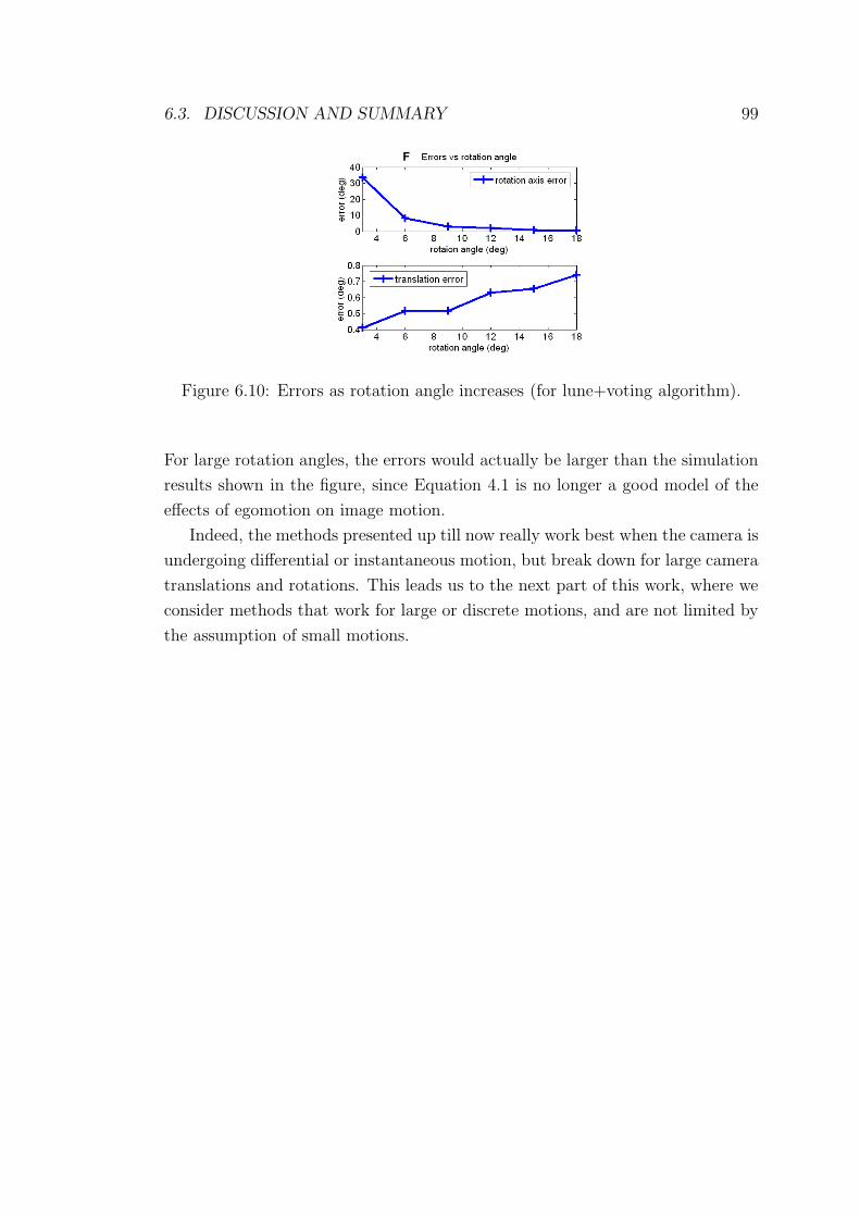
6.3. DISCUSSION AND SUMMARY 99
Figure 6.10: Errors as rotation angle increases (for lune+voting algorithm).
For large rotation angles, the errors would actually be larger than the simulation
results shown in the figure, since Equation 4.1 is no longer a good model of the
effects of egomotion on image motion.
Indeed, the methods presented up till now really work best when the camera is
undergoing differential or instantaneous motion, but break down for large camera
translations and rotations. This leads us to the next part of this work, where we
consider methods that work for large or discrete motions, and are not limited by
the assumption of small motions.

Part III
Discrete Camera Motion
101


Outline of Part III
In Part III, we consider egomotion recovery for cameras undergoing discrete mo-
tions.
1. Chapter 7: Here, we present the antipodal-epipolar constraints on rela-
tive camera motion. These make use of antipodal points to obtain separate
linear constraints for translation and rotation. Robust algorithms are in-
troduced, and their performance demonstrated with experiments.
2. Chapter 8: Next, we consider the idea of relaxed egomotion recovery,
where we relax the requirement for highly accurate estimates whilst still
remaining robust to outliers. Compared to full egomotion recovery, this
is much faster to compute, and such estimates are still useful for many
applications. We apply this idea to the problem of visual homing, where a
relaxed estimate of translation is used to perform robust robot homing in
real environments.


Chapter 7
The Antipodal-Epipolar
Constraint
Previously, in Part II, we considered egomotion recovery under the assumption
that the camera was undergoing differential motion. The main drawback with
those approaches was that their usefulness was limited to scenarios where camera
motions were small. Here in Part III, we drop this assumption and consider
discrete camera motions instead. This leads to a new formulation of the problem,
where we develop useful constraints and algorithms that work over a wider range
of camera motion sizes.
In this chapter we will introduce novel antipodal-epipolar constraints on
relative camera motion. We show that the idea of antipodal points is useful not
only under the assumption of differential motions, but also in the case of discrete
camera motions. We demonstrate the use of our constraints with two robust
and practical algorithms, one based on the RANSAC sampling strategy, and one
based on Hough-like voting. Lastly, we show that the proposed constraints work
and that the algorithms using them perform accurately and robustly in noisy
simulations and in real image sequences.
We previously saw that translation and rotation were decoupled in the motion
equations under the differential motion assumption, whereas, for the more general
discrete motion case, they were nonlinearly coupled together in the essential or
fundamental matrices (pages 37 and 42). Here, we show that even for the discrete
case, translation and rotation may be geometrically decoupled using the proper-
ties of antipodal points, allowing them to be estimated separately, independent
of each other.
In particular, through the antipodal-epipolar formulation, we can express con-
105
106 CHAPTER 7. THE ANTIPODAL-EPIPOLAR CONSTRAINT
straints that are linear in translation, and independently, constraints that are
linear in rotation. In contrast, the conventional epipolar constraint is bilinear in
translation and rotation. This is theoretically significant, as it means that under
the special condition of antipodal points, a problem that is nonlinear in general
becomes linear. This has not been achieved by any other method that we know
of.
As a result of the decoupling of motion components, we find ourselves faced
with the task of solving two smaller dimension problems instead of a single higher
dimensional one. This simplifies the task, leading to important consequences for
designing algorithms that are robust to outliers and noise. Basically, it is easier
to separate the inlier data from the outliers in a lower dimensional space than
in a higher dimensional one. This naturally results in more efficient and robust
algorithms, including ones which may be implemented to run in constant-time
regardless of outlier proportions in the data.
Furthermore, since translation can be estimated independently of rotation,
we propose a method by which one may reconstruct scene structure purely from
translation estimates, and without recovering relative camera rotation explicitly
(the rotation is implicitly constrained). This translation-only structure-from-
motion (SfM) algorithm was previously not a sensible option since past methods
recovered rotation and translation simultaneously (as the essential or fundamental
matrices). The new SfM algorithm is not only of theoretical interest but also has
practical advantages in terms of computation speed, compared to standard SfM
techniques.
In Section 7.1, we will investigate the geometry of the problem and derive
our constraints on camera motion. We present robust algorithms utilizing these
constraints in Section 7.2 and discuss our reconstruction method in Section 7.3.
Section 7.4 demonstrates the performance of our methods with some experiments
and we end with some discussion in Section 7.5.
7.1 Theory
In Figure 7.1(a), a camera centred on the point C undergoes some rigid body
motion - a translation t and rotation R - that takes it to a new position C ′ and
some new orientation. The image-spheres centered on cameras C and C ′ are
also shown. The world point P is imaged by the two cameras giving the point
correspondence p and p′. The ray −p is antipodal to p. If there happens to be

7.1. THEORY 107
(a) (b)
Figure 7.1: (a) Some translation t and rotation matrix R relates the two cameras
at C and C ′. (b) Cameras C and C ′ and world points P and Q. Rays p and q
(i.e. q = −p) are antipodal in the camera C view. p and p′ are one pair of point
correspondences and q and q′ are another. t is the translation directed from C
to C ′ in the coordinate frame of C, and t′ is directed from C ′ to C in the frame
of C ′. All points and rays shown lie on the same epipolar plane.
another world point lying on the ray −p, and that point is also visible to camera
C ′, then we can obtain antipodal-epipolar constraints on t, and on R.
Such a situation is shown in Figure 7.1(b) (essentially the same setup as (a)
but without the spheres) where a pair of world points, P and Q, project onto C
to give the rays p and q. Suppose these world points, and hence the rays, are
antipodal relative to C, that is, q = −p (where the rays are expressed in the
image coordinate frame of C).
Meanwhile, the projection of the world points onto the second camera, C ′
gives the rays p′ and q′ (i.e. the rays are expressed in the coordinate frame of
C ′). Therefore, p and p′ are a pair of point correspondences and q and q′ are
another pair.
t is the translation directed from C to C ′, expressed in the coordinate frame
of C. Conversely, t′ is the translation directed from C ′ to C, expressed in the
coordinate frame of C ′.
As before, we can only recover t (or t′) up to a scale [93], so that gives 2
unknowns to be recovered. R contains another 3 unknowns; so altogether there
are 5 unknown motion parameters to be solved for. Let all vectors denoted with
lower case letters be of unit length.

108 CHAPTER 7. THE ANTIPODAL-EPIPOLAR CONSTRAINT
7.1.1 Constraint on translation
All the points and rays in Figure 7.1(b) lie on a single plane if p and q are
antipodal. p, p′ and t lie on a plane - the epipolar plane. Likewise, q, q′ and t
also lie on a plane, and if p and q are antipodal, then the two planes are one and
the same. At first glance, it seems as though the extra pair of correspondences q
and q′ may be giving redundant information since the epipolar equation arising
from it describes the same plane as the one arising from the pair p and p′.
However, notice that we can express the equation of the epipolar plane purely
using the rays p′ and q′. The normal vector to the plane is simply given by p′×q′
where × denotes the cross product. Then, we have:
t′ T (p′ × q′) = 0 (7.1)
This is a linear constraint on the translation, t′, independent of rotation, R.
Geometrically, Equation 7.1 simply states that t′ lies on the epipolar plane. Let us
call this the antipodal-epipolar constraint on translation. (We use the ‘antipodal-’
qualifier to differentiate this from the usual epipolar constraint, p′TEp = 0, where
E is the essential matrix.) Note that if the points are antipodal in camera C, then
the constraint is on t′; conversely, if the points are antipodal in camera C ′, then
the constraint is on t.
It is also important to note that the sign of translation is unambiguously re-
coverable (whereas in normal essential matrix estimation, it is ambiguous whether
the camera translation is t or −t [93]). From Figure 7.1(b), it is clear that t′
must lie between p′ and q′, that is, (t′)Tp′ > 0 and (t′)Tq′ > 0. Hence it cannot
lie in the opposite direction.
Ambiguity arises only when both world points P and Q are infinitely far away;
then p′ and q′ will also be antipodal and it is not possible to determine the sign
of t′. Obviously, infinitely distant points can tell us nothing about translation,
and this degenerate case is easily detectable as infinitely distant P and Q means
p, q will be antipodal, and p′, q′ will also be antipodal.
A minimum of two pairs of antipodal points (which is four points), will recover
translation up to a positive scale (since the sign of t is known). One pair of
antipodal points constrains translation to lie on a plane. Another pair of antipodal
points (that do not lie on the first plane), gives another such plane, and the two
distinct planes intersect to give the direction of translation (Figure 7.2(a)).

7.1. THEORY 109
7.1.2 Constraint on rotation
The relative rotation between the two camera coordinate frames may similarly
be constrained by the epipolar planes. The ray p must lie on the plane given by
p′ × q′, so we have:
(Rp)T (p′ × q′) = 0 (7.2)
This gives a linear constraint on rotation, R, independent of the transla-
tion. Let us call this the antipodal-epipolar constraint on rotation. (Note that
(Rq)T (p′ × q′) = 0 gives no extra information as it is linearly dependent to
Equation 7.2, since p = −q).
The 3×3 rotation matrix contains effectively 3 unknowns, since RTR = I gives
6 quadratic constraints on the 9 entries of the matrix. Therefore, a minimum of
3 antipodal pairs is sufficient to recover rotation. Geometrically, this corresponds
to the situation depicted in Figure 7.2(b). However, this is a nonlinear solution.
To obtain a linear solution, one requires a minimum of 9 points to constrain the
9 entries in R.
Just as with the conventional epipolar constraint, the case of purely rotational
motion (no translation) is degenerate. This event may be easily detected as all the
antipodal points in the first camera will still be antipodal in the second camera.
This is effectively similar to the case where all world points are infinitely distant.
7.1.3 Linear and Decoupled Constraints
The conventional epipolar equation is given by:
p′T ([t]×R)p = 0 (7.3)
where the essential matrix, E, is the cross product of t and R. The equation is
bilinear in both t and R.
Contrast that with Equation 7.1, which is linear in t (and independent of
R), and with Equation 7.2 which is linear in R (and independent of t). This
demonstrates that under the special condition of antipodal points, the constraints
on motion are linear, even though the motion equations are nonlinear (or bilinear)
in general.
The decoupling of translation and rotation into separate constraint equations
leads to several advantages. For example, it means that in theory, errors in the
translation estimate will not propagate and contribute to the errors in rotation,

110 CHAPTER 7. THE ANTIPODAL-EPIPOLAR CONSTRAINT
(a) (b)
Figure 7.2: Multiple antipodal pairs give rise to multiple antipodal-epipolar
planes. Pi and Qi are pairs of antipodal world points, for i = 1, 2, 3. (a) Two
antipodal pairs give two planes that intersect to give t. (b) Three pairs give three
planes constraining the three unknowns of R.
and vice-versa. Other advantages include breaking up the problem into two lower
dimensional ones which are easier to solve. In the next section, we will see how
this naturally leads to better algorithms.
By simplifying the problem, the antipodal-epipolar constraints enable us to
explore new, robust estimation frameworks - including ones which were not at-
tractive solutions before this. The algorithms proposed will attempt to address
some of the issues or drawbacks present in existing approaches.
7.2 Robust Algorithms from Antipodal
Constraints
In this section, we present algorithms designed to be robust to outliers in the
point correspondence inputs. Like the 5-point or 8-point approaches, if greater
accuracy is desired, the output of our algorithms can be used to initialize local,
nonlinear refinement methods such as bundle adjustment [245].
Recall that in Chapter 5 we presented RANSAC and Hough-voting algorithms
(i.e. GC+RANSAC and GC+voting) that found translation from the intersection

7.2. ROBUST ALGORITHMS FROM ANTIPODAL CONSTRAINTS 111
of two or more planes. Meanwhile, in the last section, we saw that for the discrete
motion case, the recovery of translation from antipodal-epipolar constraints also
requires finding the intersection of planes. Therefore, even though the differential
and discrete cases are distinct problems, and different sets of constraints were
derived in each case, the same type of algorithms may be applied in both cases
to robustly solve for translation.
In the following, we will briefly show how the antipodal-epipolar constraint on
translation may be used within a RANSAC-type algorithm and within a Hough-
like voting algorithm. For further implementation details of each method we refer
the reader to Sections 5.2.1 and 5.2.2 of Chapter 5.
The robust recovery of translation with either RANSAC or voting also results
in the segmentation of the data into inliers and outliers. These inliers may then be
used in the next stage to recover rotation using the antipodal-epipolar constraint
on rotation1.
The algorithms presented here aim to demonstrate the viability of the novel
geometrical constraints introduced, and as such, play an illustrative role rather
than a definitive one. Many other algorithms utilizing the antipodal constraints
are possible, and the reader may replace them with their favorite robust estima-
tion method.
7.2.1 Robustly Finding Translation
RANSAC
Recall that minimal solvers are crucial for hypothesize-and-test methods such as
RANSAC and its relatives. This is because a reduction in the number of points
needed to generate a hypothesis greatly increases the probability of picking an
outlier-free set of points. This then speeds up the process significantly as the
number of hypotheses that need to be tested before a good one is found with
high probability, is reduced.
We can obtain a minimal solver requiring 2 antipodal pairs (which is 4 points).
As discussed above, the minimum number of points required to recover translation
is 2 antipodal pairs (4 points) and the minimum required to recover rotation is 3
1This actually introduces some coupling between the translation and rotation estimates.
However, the effect is not too significant and we made this design choice for efficiency pur-
poses. In general, algorithms can be devised such that the two estimates are independent, since
the constraints themselves are decoupled. For example, rotation can be found by performing
RANSAC over all points, rather than just the inliers found by the translation stage.
112 CHAPTER 7. THE ANTIPODAL-EPIPOLAR CONSTRAINT
pairs (6 points). At first glance, it therefore seems that we need a minimum of 3
pairs. However, because we can estimate translation and rotation separately, we
can actually get away with a minimum of 2 pairs instead of 3.
First, translation is found via RANSAC and a 4-point (2 pair) minimal solver.
The inlier-outlier segmentation of data points occurs at this stage - any pair
that satisfies Equation 7.1 to within some threshold is an inlier. The recovered
inliers then give an over-constrained system of homogeneous, linear equations (via
Equation 7.2) from which a least squares solution to rotation can be found.
Our antipodal point and RANSAC algorithm performs faster than the usual
5-point and RANSAC algorithm, since a smaller number of points are used for
hypothesis generation (4 versus 5 points). Further time savings are incurred due
to the fact that the solver solves a simple, linear problem of intersecting two
planes (contrast that with the tenth order polynomial that the nonlinear 5-point
algorithm needs to solve). Implementation of the required solver is trivial.
However, like all RANSAC-based methods, run-time will still increase with
increasing outlier proportions. This leads us to the next algorithm, which does
not face this problem, since it avoids random sampling altogether.
Hough-like Voting
Since translation estimation is a fairly low dimensional problem (2D), we suggest
that here, Hough-like voting may be an efficient algorithm for robust estimation.
Voting has previously been used for estimation of discrete camera motion [15,
154, 51]. However, these generally vote in some higher dimensional space (e.g.
at least 5D for estimating essential matrices). Hence, the large number of bins
needed to discretize the solution space made previous methods susceptible to the
problem of sparsity of points. Here, the decoupling effect of antipodal points
enables us to work in a 2D solution space, for which voting is both effective and
efficient.
This algorithm represents a break from previous approaches for estimating
discrete camera motion, which were largely based on the conventional epipolar
constraint and relied on robust frameworks using RANSAC-type, Monte-Carlo
hypothesis generation and testing. Voting, in contrast, performs in constant time
under increasing outlier proportions, and does so without sacrificing robustness
or accuracy (recall that to achieve speed-ups under increasing outliers, methods
such as Preemptive-RANSAC, R-RANSAC and Optimal R-RANSAC trade-off
on robustness and accuracy for run-time). Also, voting does not require the use

7.2. ROBUST ALGORITHMS FROM ANTIPODAL CONSTRAINTS 113
(a) (b)
Figure 7.3: (a) The epipolar plane Π intersects the image-sphere to give the great
circle G. (b) Result of the fine voting stage. The peak is obvious even with 60%
outliers.
of minimal point solvers.
Each antipodal pair constrains t to lie on some plane and the intersection
of two or more planes will recover t. By voting to each plane, we can robustly
find the best ray of intersection from all the planes. Instead of random sampling,
we will use the constraints arising from every antipodal pair available. This is
because voting is computationally very cheap, hence there is no reason not to use
all the available constraints.
To perform voting, we need a representation of the space in which the solutions
lie. Borrowing from our previous work in Chapters 5 and 6, we first represent the
space of possible directions of translation as the surface of a unit image-sphere
centered on the camera center. The intersection of a plane passing through the
sphere center with the surface of the sphere is a great circle. The problem of
finding the intersection of planes then becomes one of finding the intersection of
great circles on the sphere.
This is illustrated in Figure 7.3(a), where the epipolar plane Π with normal
vector p′ × q′ intersects with the surface of the unit sphere at the great circle G.
After voting along all the great circles arising from all the antipodal pairs, the
peak in the vote table gives a robust estimate of the translation.
For efficiency purposes, we perform multistage coarse-to-fine voting, first on
the sphere, and later on a projection plane. For the implementation details of
coarse voting on great circles and fine voting on straight lines, we refer the reader
to the similar voting framework used for differential camera motion estimation in

114 CHAPTER 7. THE ANTIPODAL-EPIPOLAR CONSTRAINT
Chapter 5. Figure 7.3(b) shows an example of the fine voting stage. The peak is
obvious even with 60% outliers in the data (this is a window of the voting space
and many more outliers lie outside the window).
Once again, a natural consequence of translation estimation is the segmenta-
tion of inliers from outliers in the data. Points that resulted in straight lines (in
the fine voting stage) that pass through the translation estimate are inliers (i.e.
equivalent to satisfying Equation 7.1). A last linear refinement step is performed
using these inliers in order to obtain a least squares estimate of translation. This
last step mitigates the effects of voting bin quantization on accuracy.
7.2.2 Finding Rotation from the Linear Constraints
Using only the inliers found when estimating translation with either the RANSAC-
based or voting-based methods above, we now go on to perform rotation estima-
tion with Equation 7.2, which is linear in rotation, R. Each pair of inlier points
would give one linear constraint on rotation. M inliers will give M linear con-
straints, giving a system of over-constrained equations which may be written in
the form A[Rvec] = 0, where [Rvec] is the vectorized form of the rotation matrix,
R. A is a M × 9 matrix, whilst [Rvec] is a 9 × 1 vector.
To be able to solve for R linearly, we need M ≥ 9. A[Rvec] = 0 can then be
solved by the DLT algorithm [93], which involves performing a SVD, A = UDVT .
The least-squares solution is given by the column of V corresponding to the
smallest singular value in D. A final nonlinear correction step ensures R is a
‘proper’ rotation matrix by enforcing RRT = I and det(R) = 1 (so the complete
method for rotation recovery is linear except for this final correction step).
In practice, there is a small, but finite probability of outliers slipping past
the outlier rejection stage during translation estimation. This happens when the
outlier is a ‘leverage point’ that satisfies the translation constraint of Equation 7.1
but does not satisfy the constraints of full camera motion. Therefore, a practical
system may need another RANSAC stage (or other robust algorithm) here. Since
the vast majority of outliers (usually all) have been removed, this step generally
happens quickly, i.e. terminates in one iteration2. In the event of one or two
leverage points slipping in, the RANSAC stage will then detect and deal with
them.
2Since we know the outlier probability is very low, we did not use a nonlinear minimal-point
rotation solver since RANSAC will undergo few iterations. Such a minimal-point rotation solver
is a possible alternative but it is harder to implement compared to the method used here.
7.3. STRUCTURE FROM PARTIAL-MOTION 115
Another factor to take into practical consideration is the size of singular values
found in the SVD. Certain singular values in the diagonal matrix, D, can some-
times be very small, and under noise, it can be hard to distinguish the smallest
singular value. To remedy this, we test all solutions corresponding to very small
singular values by reconstructing several points, and picking the solution where
all reconstructed points are in front of both cameras (similar to the test applied
to disambiguate twisted-pairs in essential matrix motion recovery [93]).
7.3 Structure from Partial-Motion - Not Find-
ing Full Rotation
One observes that relative scene structure can actually be found without recover-
ing the parameters of rotation. Previously, this fact was not particularly useful,
since conventional epipolar geometry methods will recover translation and ro-
tation simultaneously, that is, they are entangled together in the essential or
fundamental matrices which are to be estimated.
Here, however, the two are found separately. Therefore, if the goal of some
system was structure recovery, then there is no necessity to compute any extra
parameters which are not needed for the task. In particular, we will show that
recovering translation twice, that is, finding t and t′, is sufficient for structure
computation. Rotation is not explicitly estimated at all.
Computing t and t′ amounts to recovering rotation up to 1 degree of freedom.
t and t′ both lie on the straight line, CC ′, joining the camera centers. If t and
t′ have been found, the two cameras are still free to rotate relative to each other
about the axis CC ′. However, given a point correspondence, we can assume
that the rays p and p′ intersect at the world point P. This implicitly constrains
the last remaining degree of freedom of rotation (without having to explicitly
estimate it).
Figure 7.4 shows the geometry of the situation. t is estimated from points
which are antipodal in camera C ′, whilst t′ is found from points which are an-
tipodal in camera C. Then, from basic trigonometry, we have:
tan(α) =Zl
Xl
, tan(β) =Zr
Xr
, Xr = |T| − Xl (7.4)
where |T| is the baseline, the magnitude of which, we set to unit. α = acos(tTp)
and β = acos(t′ Tp′) where all ray vectors are unit length. With |Zr| = |Zl| = Z,
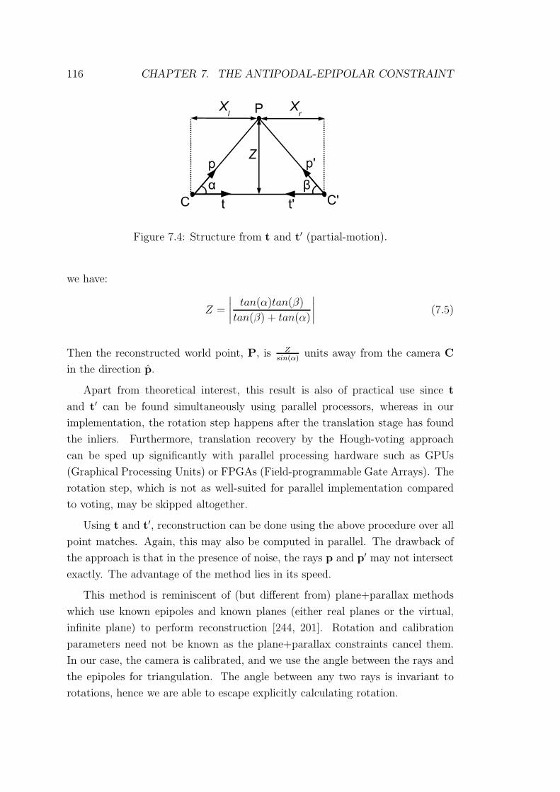
116 CHAPTER 7. THE ANTIPODAL-EPIPOLAR CONSTRAINT
Figure 7.4: Structure from t and t′ (partial-motion).
we have:
Z =
∣
∣
∣
∣
tan(α)tan(β)
tan(β) + tan(α)
∣
∣
∣
∣
(7.5)
Then the reconstructed world point, P, is Zsin(α)
units away from the camera C
in the direction p.
Apart from theoretical interest, this result is also of practical use since t
and t′ can be found simultaneously using parallel processors, whereas in our
implementation, the rotation step happens after the translation stage has found
the inliers. Furthermore, translation recovery by the Hough-voting approach
can be sped up significantly with parallel processing hardware such as GPUs
(Graphical Processing Units) or FPGAs (Field-programmable Gate Arrays). The
rotation step, which is not as well-suited for parallel implementation compared
to voting, may be skipped altogether.
Using t and t′, reconstruction can be done using the above procedure over all
point matches. Again, this may also be computed in parallel. The drawback of
the approach is that in the presence of noise, the rays p and p′ may not intersect
exactly. The advantage of the method lies in its speed.
This method is reminiscent of (but different from) plane+parallax methods
which use known epipoles and known planes (either real planes or the virtual,
infinite plane) to perform reconstruction [244, 201]. Rotation and calibration
parameters need not be known as the plane+parallax constraints cancel them.
In our case, the camera is calibrated, and we use the angle between the rays and
the epipoles for triangulation. The angle between any two rays is invariant to
rotations, hence we are able to escape explicitly calculating rotation.

7.4. EXPERIMENTAL RESULTS 117
7.4 Experimental Results
We now demonstrate that the antipodal-epipolar constraints work, and that the
algorithms based on them work robustly and accurately in practice. We run
tests on the translation estimation algorithms (which, for brevity, we term as
the ‘antipodal+RANSAC’ and ‘antipodal+voting’ methods), as well as on our
algorithm for recovering rotation (referred to as ‘antipodal’ in the legends of the
graphs for errors in rotation). The results for simulations under outliers and noise
are shown in Figures 7.5 and 7.7; whilst results for real image experiments are in
Figure 7.8.
Results were benchmarked against the performance of 5point+RANSAC, which
consists of the 5-point algorithm of Li and Hartley [136] within the RANSAC code
of [127] (see Section 3.1.5, for details of RANSAC). As before, the algorithm will
estimate the outlier probability from the sampled data and use that to adaptively
determine the amount of samples required such that the statistical probability
of sampling at least one outlier free measurement is p = 0.99. We tested using
Sampson distance thresholds of 0.01 and 0.005 (the experiments will demonstrate
the effects of lowering the threshold from 0.01 to 0.005 on RANSAC’s robustness
to outliers and on its run-time).
The antipodal+RANSAC method also worked with the RANSAC code of
[127]. Adaptive sampling probability was p = 0.99 and the threshold used was
0.5◦ (angle between translation and the antipodal-epipolar plane). The antipo-
dal+voting method performed coarse-to-fine voting in two stages, with the esti-
mate taken as the centre of mass of voting bin(s) with the highest votes.
We measure the accuracy of the estimates on translation direction, rotation
axis and rotation angle. All errors are measured in units of degrees (e.g. the angle
between the true and estimated translation directions). All algorithms used were
Matlab implementations.
7.4.1 Simulations
Method: A series of simulated experiments were performed in Matlab to test
performance under increasing outlier proportions and under increasing Gaussian
noise. Two views of a 3D scene were generated with random translations and
rotations between cameras. The magnitude of the translation varied randomly
between 5 and 10 units; the rotation angle varied randomly between 10◦ and 50◦;
whilst the distances to the world points varied between 5 and 10 units. Results

118 CHAPTER 7. THE ANTIPODAL-EPIPOLAR CONSTRAINT
0 0.1 0.2 0.3 0.4 0.5 0.60
0.05
0.1
0.15
0.2
0.25
0.3
0.35
0.4
0.45
0.5
Outlier Proportion
Err
or
(de
g)
Translation Error (deg) vs Outlier Proportions
5pt+RANSAC (t = 0.01)
5pt+RANSAC (t = 0.005)
antipodal+voting
antipodal+RANSAC
(a)
0 0.1 0.2 0.3 0.4 0.5 0.60
0.2
0.4
0.6
0.8
1
1.2
1.4
1.6
1.8
2
Outlier Proportion
Err
or
(deg)
Rotation Axis Error (deg) vs Outlier Proportion
5pt+RANSAC (t = 0.01)
5pt+RANSAC (t = 0.005)
antipodal
(b)
0 0.1 0.2 0.3 0.4 0.5 0.60
0.1
0.2
0.3
0.4
0.5
0.6
0.7
0.8
Outlier Proportion
Err
or
(de
g)
Rotation Angle Error (deg) vs Outlier Proportion
5pt+RANSAC (t = 0.01)
5pt+RANSAC (t = 0.005)
antipodal
(c)
Figure 7.5: Errors under increasing outlier proportion. All methods performed
robustly, giving small errors for outlier proportions of up to 60%. However,
our methods gave much smaller increases in error compared to the benchmark
approach. Here, t is the Sampson distance threshold used for 5-point+RANSAC.
were averaged over 100 trials.
We tested on data contaminated with outliers in proportions ranging from
10% to 60%; and on data under Gaussian noise with zero mean and standard
deviations of up to 0.3◦ (In a camera with viewing angle 60◦ and a 640x480 pixel
image, 0.3◦ corresponds to around 2 to 3 pixels of noise). This corresponds to
realistic noise levels in feature matching methods (e.g. SIFT), which are sub-
pixel accurate and typically exhibit errors of at most a couple of pixels. Outliers
consisted of randomly mismatched rays, whilst Gaussian noise was simulated by
perturbing the directions of image rays according to a Gaussian distribution.
Robustness to Outliers: The antipodal point algorithms proved to be
remarkably resistant to increasing outlier proportions. Figures 7.5(a-c) demon-
strate that increasing the outlier proportions up to 60%, caused little appreciable
increase in the error of motion estimates from the antipodal+voting and antipo-
dal+RANSAC methods. Over the same increase in outliers, the errors for the
5-point+RANSAC method were still small, but increased more quickly compared
to our methods.
The improved outlier robustness of our methods compared to 5-point+RANSAC
is not an unusual result since our methods perform robust estimation in a 2-
dimensional space instead of a higher, 5-dimensional one. It is simply more effi-
cient and effective to perform the task of clustering inliers from outliers in a lower
dimensional space. Also, since each constraint used less points compared to the
5-point algorithm, the probability of obtaining a good constraint is significantly
increased, which is important for the sampling done in the antipodal+RANSAC
framework. Similar improvements in robustness were also observed in Part II for

7.4. EXPERIMENTAL RESULTS 119
our algorithms that estimated differential camera motion.
0 0.1 0.2 0.3 0.4 0.5 0.60
10
20
30
40
50
60
70
Outlier Proportion
Tim
e (
sec)
Processing Time (sec) vs Outlier Proportion
antipodal+voting
antipodal+RANSAC
5pt+RANSAC
(a)
0 0.1 0.2 0.3 0.4 0.5 0.60.8
0.85
0.9
0.95
1
1.05
1.1
1.15
Outlier Proportion
Tim
e (
sec)
Processing Time (sec) for both our methods
antipodal+RANSAC
antipodal+voting
(b)
Figure 7.6: (a) Run-time versus increasing outlier proportion. (b) Using a smaller
scale for the y-axis (zooming in) to compare the performance of the two antipodal
methods.
Run-time: It is important to keep in mind that the above results for the
antipodal+voting method happened in constant processing time regardless of the
outlier proportion in the data3. In contrast, Figure 7.6(a) shows that the time
taken for 5-point+RANSAC to arrive at a good solution increased quickly with
increasing outlier proportions. Meanwhile, Figure 7.6(b) compares the timing
for the antipodal+RANSAC and antipodal+voting methods. We see that run-
time for antipodal+RANSAC also increased, but at a slower rate compared to
5-point+RANSAC, since it uses less points and solves a much simpler, intersection
of two planes problem. The numbers in the graphs are obviously implementation
dependent, but the trend will remain the same.
As outlier proportion increases, RANSAC increases the number of solutions,
N , that are evaluated and tested, in order to maintain a high chance of hitting on
a good one. N is adaptively increased according to N = log(1 − p)/log(1 − qs),
where the number of points needed for generating a solution is s = 5 for the
5-point algorithm. q is the inlier probability, and p is the probability of there
being at least one sample of outlier-free points in the N samples chosen. The
antipodal+RANSAC algorithm also faces the same problem of increasing run-
time but the increase is less rapid.
Another parameter influencing RANSAC processing time is the distance thresh-
old used for distinguishing outliers from inliers. If the threshold is made stricter,
3The run-time behaviour of antipodal+voting is similar to that observed in the tests on
voting algorithms for finding differential egomotion in Chapter 6.

120 CHAPTER 7. THE ANTIPODAL-EPIPOLAR CONSTRAINT
the errors in the estimate may be further lowered. For example, in Figure 7.5,
by reducing the distance threshold of 5point+RANSAC from 0.01 to 0.005, the
error is improved in general. However, RANSAC will then have to iterate many
more times and take even longer to obtain the solution.
Our implementation of the antipodal+voting method is constant-time because
the approach is sufficiently fast such that using all the constraints arising from
every antipodal pair is viable. Also, if M antipodal pairs are available, there are
only M antipodal-epipolar constraints to consider. Hence the run-time is linear
in the number of antipodal points used for estimation.
0 0.05 0.1 0.15 0.2 0.25 0.30
0.05
0.1
0.15
0.2
0.25
0.3
0.35
0.4
0.45
0.5
Gaussian noise std dev (deg)
Err
or
(de
g)
Translation Error (deg) vs Gaussian Noise
5pt+RANSAC
antipodal+voting
antipodal+RANSAC
(a)
0 0.05 0.1 0.15 0.2 0.25 0.30
0.05
0.1
0.15
0.2
0.25
0.3
Gaussian noise std dev (deg)
Err
or
(deg)
Rotation Axis Error (deg) vs Gaussian Noise
5pt+RANSAC
antipodal
(b)
0 0.05 0.1 0.15 0.2 0.25 0.30
0.02
0.04
0.06
0.08
0.1
Gaussian noise std dev (deg)
Err
or
(deg)
Rotation Angle Error (deg) vs Gaussian Noise
5pt+RANSAC
antipodal
(c)
Figure 7.7: Performance degrades gracefully under increasing Gaussian noise.
Gaussian Noise: Figures 7.7(a-c) show that all methods tested gave small er-
rors, with performance degrading gracefully under increasing Gaussian noise. Fig-
ure 7.7(a) shows that errors for the translation estimates of antipodal+RANSAC
were about similar to that of 5-point+RANSAC. Translation errors from antipo-
dal+voting were slightly higher (less than 0.2◦ difference) due to quantization er-
ror from dividing the solution space into a finite set of voting bins; its performance
may be improved by voting with finer resolutions (we used only 2 coarse-to-fine
stages). The errors for rotation axis and angle in 7.7(b-c) were also comparable
to 5-point+RANSAC.
7.4.2 Real Image Sequences
Method: Experiments were conducted with real image sequences obtained
from a Ladybug omnidirectional camera [187]. In Image Sequence A, the camera
was placed on the ground, where it translated by about 4cm and rotated by 10◦
between frames. The scene was static. The motion was estimated and compared
with measured ground truth values. Figures 7.9(a-e) show the images captured
by the Ladybug omnidirectional camera rig at one time instance in sequence A.

7.4. EXPERIMENTAL RESULTS 121
1 3 5 7 9 11 13 150
1
2
3
4
5
6
7
8
9
10
11
Frame No.
Err
or
(deg)
A. Translation Error (static scene)
antipodal+voting
antipodal+RANSAC
5pt+RANSAC
(a)
1 3 5 7 9 11 13 150
0.5
1
1.5
2
2.5
3
3.5
4
4.5
5
Frame No.
Err
or
(deg)
A. Rotation Axis Error (static scene)
antipodal
5pt+RANSAC
(b)
1 3 5 7 9 11 13 150
0.5
1
1.5
2
2.5
3
3.5
4
4.5
5
Frame No.
Err
or
(deg)
A. Rotation Angle Error (static scene)
antipodal
5pt+RANSAC
(c)
1 3 5 7 9 11 13 150
1
2
3
4
5
6
Frame No.
Err
or
(deg)
B. Translation Error (moving objects)
antipodal+voting
antipodal+RANSAC
5pt+RANSAC
(d)
1 3 5 7 9 11 13 151
2
3
4
5
6
7
8
9
10
Frame No.
Err
or
(deg)
B. Rotation Axis Error (moving objects)
antipodal
5pt+RANSAC
(e)
1 3 5 7 9 11 13 150
0.2
0.4
0.6
0.8
1
1.2
1.4
1.6
1.8
2
Frame No.
Err
or
(deg)
B. Rotation Angle Error (moving objects)
antipodal
5pt+RANSAC
(f)
Figure 7.8: Experiments on real images. (a-c) Image Sequence A - static scene,
translation 4cm, rotation 10◦ per frame. (d-f) Image Sequence B - dynamic scene
containing moving objects, translation 4cm, rotation 4◦ per frame.
122 CHAPTER 7. THE ANTIPODAL-EPIPOLAR CONSTRAINT
In another experiment, Image Sequence B, the camera translated by 4cm and
rotated by 4◦ between frames; furthermore, the scene contained independently
moving objects, leading to greater outlier probabilities. Also, the fact that motion
was planar, was not used by any of the algorithms to simplify estimation.
Note that these are the same sequences tested on the GC+RANSAC and
GC+voting algorithms which also find intersections of planes (Section 6.2.3).
The difference is that here, we skipped every alternate frame in order to obtain
larger camera motions between frames.
SIFT features (code from [143]) were used to find point correspondences. In
the real images, several hundred antipodal points can typically be found, which
are many more than the minimum needed. Points that are within 0.5◦ of being
antipodal are approximated as antipodal.
Motion Estimates: Figures 7.8 (a-c) show errors for image sequence A
(static scene) whilst Figures 7.8 (d-f) show errors for sequence B (contains moving
objects). In these experiments, the three methods performed comparably. The
differences in average errors of all three methods were small - less than 1◦ - which
is within the bounds of the accuracy of our ground truth measurements.
The accuracy of all methods were affected by practical issues such as the
fact that the Ladybug camera rig is only approximately central - the centres of
its constituent cameras dont exactly coincide. Also, our methods approximated
nearly antipodal points to be antipodal. In spite of this additional source of error,
our methods performed comparably to 5-point.
The rotation angle in sequence A (10◦) was larger than in sequence B (4◦), re-
sulting in better rotation estimates and worse translation estimates for A (and the
reverse for results of B). Videos showing the experiments and recovered estimates
are included as supplementary material (see Appendix A).
7.4.3 Structure Estimates
Our structure from partial-motion method is compared with a standard linear
triangulation method (see [92, 93] for details) in simulations under noise and in
reconstructions of real scenes.
Under increasing Gaussian noise, the simulation results of Figure 7.9(f) show
that our partial-motion method and linear triangulation performed comparably,
with both giving small average reconstruction errors. Both methods used true
camera motions and noisy correspondence data as inputs. Errors were measured
as the Euclidean distance between a reconstructed point and the (scaled) true

7.4. EXPERIMENTAL RESULTS 123
(a) (b) (c) (d) (e)
0 0.1 0.2 0.3 0.4 0.50
0.002
0.004
0.006
0.008
0.01
0.012
0.014
0.016
0.018
Gaussian noise std dev (deg)
Err
or
(un
its)
Reconstruction Error vs Gaussian Noise
our method
standard triangulation
(f)
−25 −20 −15 −10 −5 0 5 10 15 20 25−25
−20
−15
−10
−5
0
5
10
15
20
25
(g)
−25 −20 −15 −10 −5 0 5 10 15 20 25−25
−20
−15
−10
−5
0
5
10
15
20
25
(h)
Figure 7.9: (a-e) Example images from Image Sequence A taken by the 5 cam-
eras on the Ladybug omnidirectional camera rig. (f) Gaussian noise simulation
comparing our partial-motion structure method with standard linear triangula-
tion. (g-h) Top-down view of structure estimates for Image Sequence A using our
method and using linear triangulation respectively, with ground truth motion as
the inputs. Points on the ground are marked red and points corresponding to
objects above the ground are marked blue.
124 CHAPTER 7. THE ANTIPODAL-EPIPOLAR CONSTRAINT
world point.
We also performed reconstruction on Image Sequence A, and Figure 7.9(g-
h) shows a bird’s eye view of the reconstructed environment. Using measured
ground truth motion as inputs, both methods gave very similar reconstructions.
Blue denotes points belonging to objects above the ground whilst points on the
ground are marked red.
All plots show results before performing any nonlinear refinement, which can
be applied here to improve accuracy. The scale of the plotted structure is arbitrary
since it is not recoverable.
7.5 Discussion
Real-time implementations: Like our previous voting implementations, the
antipodal+voting algorithm is also fundamentally parallel, and implementation
on a GPU or FPGA should further speed it up as the hardware would be able
to take advantage of this. Furthermore, since it works in constant-time under in-
creasing outliers, it can potentially give robust, fast performance even in complex
scenes with large, variable outlier proportions.
Decoupling leads to improved algorithms: Motion decoupling leads to
novel algorithms that were previously not efficient or not possible for estimat-
ing the discrete camera motions. For example, bringing the problem down to
lower dimensions enabled us to efficiently perform Hough-voting. It also led to
the structure from partial-motion algorithm, which saves time by not having to
explicitly find rotation.
Further improvements on accuracy: Whilst the results show that the
methods discussed give accurate motion estimates, further linear and nonlinear
refinement may be performed to obtain even more accurate results. Once trans-
lation and rotation have been estimated, all inlier points may be used to linearly
refine the estimated motions (whereas in the experiments above, linear refine-
ment was performed using only the inlier antipodal points and points without
antipodes were not used). Further refinement using nonlinear techniques such as
bundle adjustment are also standard.
Effect of motion size: Figures 7.10(a-b) show the effects of different mag-
nitudes of camera motion. In (a), as the magnitude of translation increases,
the translation is estimated with increasing accuracy. Conversely, in (b), as the
rotation angle becomes small, rotation is increasingly difficult to recover. These

7.6. DISCRETE VERSUS DIFFERENTIAL 125
effects are in accordance with the behavior of virtually all other motion estimation
methods.
Finding antipodal points efficiently: In our experiments, we searched
through all available correspondences for antipodes, which is not very efficient.
(Recall that in Section 6.2.1, for differential motions, we were able to efficiently
obtain antipodal flow via the Lucas-Kanade method. However, for large discrete
motions, this method is not suitable.) For a faster method, we recommend avoid-
ing this search by using DAISY features [236]. Whilst SIFT features are meant
to be computed only at certain positions in the image (at the local extrema in
a stack of Difference-of-Gaussian images), DAISY features are designed to be
computed anywhere in the image. The antipodal points can then be chosen in
advance and the DAISY descriptor is computed at those points.
Deterministic solutions: It is interesting to note that the solution given
by RANSAC is random - i.e. 100 different runs can give 100 different solutions
scattered around the ‘true’ solution. This happens since sampling is random, so
slightly different sets of inliers will be found each time [135]. On the other hand,
the voting approach suggested here gives deterministic solutions since random
sampling is not used.
0 2 4 6 8 10 12 140.12
0.13
0.14
0.15
0.16
0.17
0.18
0.19
0.2
0.21
Translation Magnitude (units)
Err
or
(deg)
Translation Error (deg) vs Translation Size
Gaussian noise std dev = 0.1 deg
(a)
0 10 20 30 40 500
5
10
15
20
25
Err
or
(de
g)
Rotation Angle (deg)
Rotation Axis Error (deg) vs Rotation Angle
Gaussian noise std dev = 0.1 deg
(b)
Figure 7.10: Performance for different motion sizes.
7.6 Discrete versus Differential
There has been some debate over the range of translation magnitudes or baselines,
for which discrete egomotion methods work. It was initially believed that discrete
egomotion methods may become less stable under very small (i.e. near differential)
motions. Recently however, some researchers have suggested that, under small

126 CHAPTER 7. THE ANTIPODAL-EPIPOLAR CONSTRAINT
camera motions, discrete motion methods work well and may even outperform
differential methods [119, 138, 243, 152, 20]4.
For example, Lin et al. [138] showed that under certain conditions and the
assumption of proportional noise, the discrete 8-point algorithm may perform
similarly for both small and large motions. Also, in simulations under differential
camera motion, they found that three variants of the discrete 8-point algorithm
[87, 168, 141] performed better than the differential methods of Ma et al. [149],
and of Jepson and Heeger [114]. The main reasons cited by the authors for the
poor performance of those differential methods were the bas-relief ambiguity and
the forward bias.
In view of these findings, this section seeks to compare the performance of our
discrete and differential antipodal constraints via simulations with different mo-
tion sizes. In particular, we consider the differential antipodal constraint obtained
by summing antipodal flow (Chapter 5) and the discrete antipodal-epipolar con-
straint discussed earlier in this chapter, since the two methods are geometrically
dual to each other - i.e. they both involve finding translation from the intersection
of multiple planes. In the following, we will refer to these as the ‘sum-antipodal’
and ‘antipodal-epipolar’ constraints respectively.
In this set of simulations, the level of Gaussian noise used was fairly small and
there were no outliers present. Hence, outlier rejection schemes like RANSAC
and voting were not used. From the image motion observed at 100 antipodal
points, the differential sum-antipodal and discrete antipodal-epipolar constraints
each gave a set of equations for which least squares solutions to translation were
found.
We also compared performance with a discrete method for linearly recovering
the essential matrix, termed ‘discrete essential matrix’. With the same set of point
correspondences (a total of 200 points, since there were 100 antipodal pairs), the
conventional epipolar constraint gave a system of linear equations from which a
least squares solution to the essential matrix may be found by the DLT algorithm.
The translation was then extracted from the matrix.
Figures 7.11(a-c) show the effects of decreasing translation baseline by several
orders of magnitude, on the performance of the three approaches. The distance
4Such research lends credence to our use of the discrete 5-point algorithm as a benchmark
against which we compared both our differential and discrete antipodal constraints in earlier
sections. Note that, to be on the safe side, we did ensure that all experiments involving 5-point
used motion sizes that were not overly small. The resulting performance for 5-point was quite
good in all the experiments.
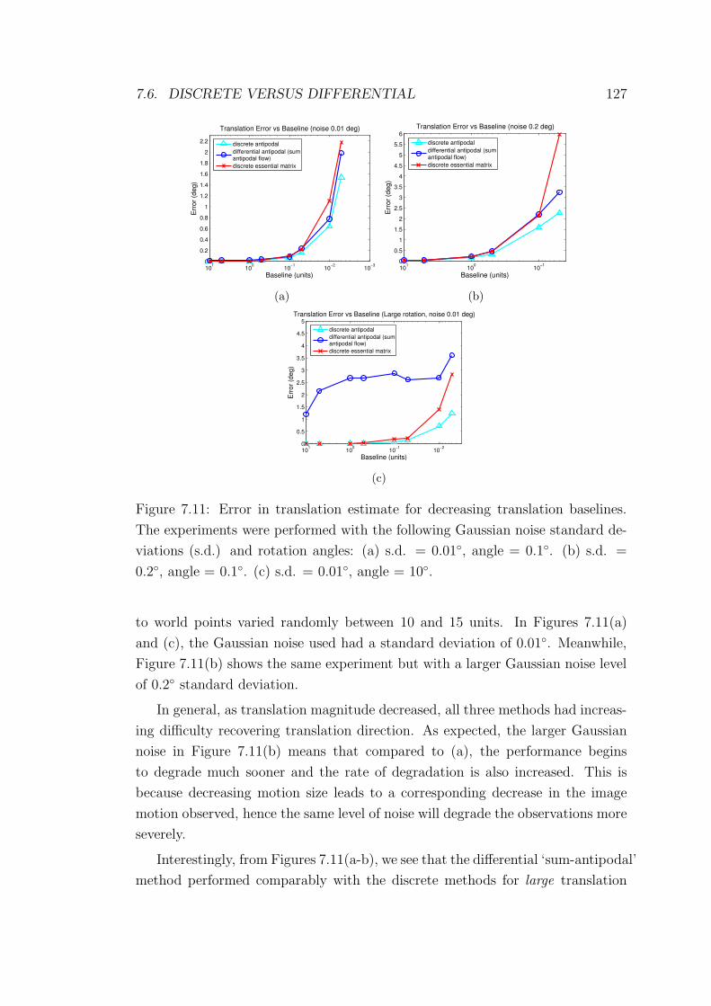
7.6. DISCRETE VERSUS DIFFERENTIAL 127
10−3
10−2
10−1
100
101
0
0.2
0.4
0.6
0.8
1
1.2
1.4
1.6
1.8
2
2.2
Baseline (units)
Err
or
(deg)
Translation Error vs Baseline (noise 0.01 deg)
discrete antipodal
differential antipodal (sumantipodal flow)
discrete essential matrix
(a)
10−1
100
101
0
0.5
1
1.5
2
2.5
3
3.5
4
4.5
5
5.5
6
Baseline (units)
Err
or
(deg)
Translation Error vs Baseline (noise 0.2 deg)
discrete antipodal
differential antipodal (sumantipodal flow)
discrete essential matrix
(b)
10−2
10−1
100
101
0
0.5
1
1.5
2
2.5
3
3.5
4
4.5
5
Baseline (units)
Err
or
(de
g)
Translation Error vs Baseline (Large rotation, noise 0.01 deg)
discrete antipodal
differential antipodal (sumantipodal flow)
discrete essential matrix
(c)
Figure 7.11: Error in translation estimate for decreasing translation baselines.
The experiments were performed with the following Gaussian noise standard de-
viations (s.d.) and rotation angles: (a) s.d. = 0.01◦, angle = 0.1◦. (b) s.d. =
0.2◦, angle = 0.1◦. (c) s.d. = 0.01◦, angle = 10◦.
to world points varied randomly between 10 and 15 units. In Figures 7.11(a)
and (c), the Gaussian noise used had a standard deviation of 0.01◦. Meanwhile,
Figure 7.11(b) shows the same experiment but with a larger Gaussian noise level
of 0.2◦ standard deviation.
In general, as translation magnitude decreased, all three methods had increas-
ing difficulty recovering translation direction. As expected, the larger Gaussian
noise in Figure 7.11(b) means that compared to (a), the performance begins
to degrade much sooner and the rate of degradation is also increased. This is
because decreasing motion size leads to a corresponding decrease in the image
motion observed, hence the same level of noise will degrade the observations more
severely.
Interestingly, from Figures 7.11(a-b), we see that the differential ‘sum-antipodal’
method performed comparably with the discrete methods for large translation
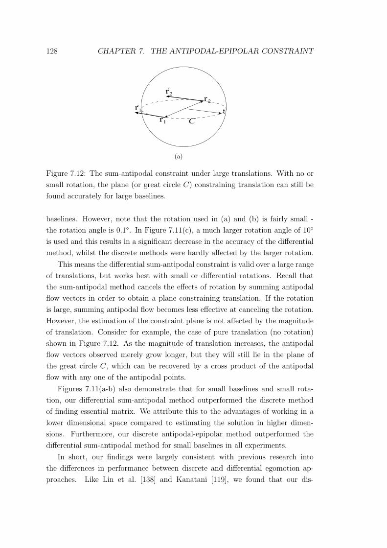
128 CHAPTER 7. THE ANTIPODAL-EPIPOLAR CONSTRAINT
(a)
Figure 7.12: The sum-antipodal constraint under large translations. With no or
small rotation, the plane (or great circle C) constraining translation can still be
found accurately for large baselines.
baselines. However, note that the rotation used in (a) and (b) is fairly small -
the rotation angle is 0.1◦. In Figure 7.11(c), a much larger rotation angle of 10◦
is used and this results in a significant decrease in the accuracy of the differential
method, whilst the discrete methods were hardly affected by the larger rotation.
This means the differential sum-antipodal constraint is valid over a large range
of translations, but works best with small or differential rotations. Recall that
the sum-antipodal method cancels the effects of rotation by summing antipodal
flow vectors in order to obtain a plane constraining translation. If the rotation
is large, summing antipodal flow becomes less effective at canceling the rotation.
However, the estimation of the constraint plane is not affected by the magnitude
of translation. Consider for example, the case of pure translation (no rotation)
shown in Figure 7.12. As the magnitude of translation increases, the antipodal
flow vectors observed merely grow longer, but they will still lie in the plane of
the great circle C, which can be recovered by a cross product of the antipodal
flow with any one of the antipodal points.
Figures 7.11(a-b) also demonstrate that for small baselines and small rota-
tion, our differential sum-antipodal method outperformed the discrete method
of finding essential matrix. We attribute this to the advantages of working in a
lower dimensional space compared to estimating the solution in higher dimen-
sions. Furthermore, our discrete antipodal-epipolar method outperformed the
differential sum-antipodal method for small baselines in all experiments.
In short, our findings were largely consistent with previous research into
the differences in performance between discrete and differential egomotion ap-
proaches. Like Lin et al. [138] and Kanatani [119], we found that our dis-

7.7. SUMMARY 129
crete antipodal-epipolar method performed as well or better than the differential
method for small motions. However, unlike Lin et al. [138], where the differential
methods tested performed very poorly due to large errors caused by the bas-relief
ambiguity and the forward bias problem, our differential sum-antipodal method
worked quite well for small motions, surpassing the discrete essential matrix ap-
proach. This is because the large FOV used by antipodal point methods means
that the bas-relief problem was virtually non-existent. Also, due to the image
sphere formulation, our method is unaffected by forward bias (refer Section 3.1.4,
page 43).
7.7 Summary
The main contribution of this chapter was the antipodal-epipolar constraint on
camera motion. We demonstrated that the geometry of antipodal points resulted
in linear, decoupled constraints on the translational and rotational components
of motion. We also showed that the antipodal-epipolar constraint works quite
well for both large and small motions.
We demonstrated the use of our constraints within the antipodal+RANSAC
algorithm which is trivial to implement, and shows improvements in robustness
to outliers and in performance time compared to the state-of-the-art. The second,
Hough-voting algorithm showed similar improvements, with the added advantage
of being well suited for implementation on a parallel machine.
We believe the decoupling of motion components simplifies the problem, and
the advantages of this were demonstrated in the novel algorithms proposed for
finding motion and estimating structure. This feature may be further exploited
in other applications as well - for example, certain camera odometry applications
do not strictly require rotation recovery, and a similar algorithm that skips find-
ing rotation may be possible, leading to speedier estimation. Conversely, if an
application needs to recover rotation (e.g. for attitude stabilization of a flying
vehicle) then translation estimation may be skipped and only rotation is found.


Chapter 8
Relaxed Egomotion and Visual
Homing
8.1 Introduction
In this chapter, we look at the problem of estimating observer egomotion from
a slightly different perspective. Previously, we have been preoccupied with ob-
taining estimates of egomotion as accurately as possible. Here, however, we look
at what we term relaxed egomotion, where we relax requirements for high
accuracy in the egomotion estimates whilst still maintaining stable and robust
performance under outliers. This generally leads to a simpler problem which may
be easier and faster to solve. We will study the usefulness of these considerably
less accurate estimates in the context of visual navigation.
In fact, we have already encountered this idea of relaxed egomotion in the
previous chapters of this work. Earlier, we saw how voting along constraint
regions (lunes, great circles and straight lines) led to a probability map of the
solution space, where more likely solutions had higher votes and the best solution
had the most votes. We mentioned that if a single, sharp peak in the voting
distribution could not be obtained, then the result obtained was less accurate
and precise, but still correct in the sense that the true solution lay within the set
of bins with maximum votes (we called this the ‘fail-soft’ property of the voting
approach, page 74). See Figure 8.1.
This is a relaxed egomotion estimate - a robust but less accurate answer with
known uncertainty is obtained. The uncertainty is bounded by how many bins
of maximum vote there are and how widely spread out they are over the solution
space. As long as certain bounds on uncertainty are met - i.e. it is not too large
131

132 CHAPTER 8. RELAXED EGOMOTION AND VISUAL HOMING
(a) (b) (c)
Figure 8.1: Shaded bins indicate voting bins with maximum vote. (a) Voting
bins are a discretized representation of the solution space. If bin A1 had the most
votes, the solution may lie in the shaded region x2 < x < x3 and y3 < y < y4.
(b) However, if more than one bin has the highest vote, then the set of possible
solutions is the union of all such bins (not necessarily a connected set). The
solution then lies with maximum probability in the region A1 ∪ A2 ∪ A3 ∪ A4
∪ A5. (c) The uncertainty in the estimate is bounded by the smallest circle
encompassing all bins with highest votes, that is, the diameter of that circle (=
2r) is the largest error possible (for example, when a point on one of the upper
vertices of bin A4 is picked as the estimate but the true solution is a point on
one of the lower vertices of A5).
- this relaxed estimate is useful for many applications and navigational tasks.
This approach has the advantage of faster estimation and lower computational
demands, which may be useful for small robots with limited payloads. For ex-
ample, small quadrotor aircraft with 250g-300g payloads [53], or microflyers that
weigh only 10g-30g in total [282, 267], would carry limited computing power on
board and may benefit from simple and cheap homing algorithms.
Alternatively, a system could give a fast and rough answer first, and later
return with a more accurate answer after further processing. This would be
a coarse-to-fine approach, with the relaxed egomotion method giving a coarse
estimate first; and one of the conventional egomotion estimation algorithms giving
an accurate and precise answer later.
Here, we will consider relaxed egomotion in the context of a visual homing
application. Given two views of the world - the home view and the current view
- a visual homing algorithm attempts to infer directions to move in, that would
take the agent from the current location, C, to its desired home location, G

8.1. INTRODUCTION 133
(a)
Figure 8.2: Visual homing: whilst−→CG gives the most direct path home, continual
updates of relaxed egomotion estimates can still get a robot home, albeit with
a less direct path. This reduces the computational burden of having to obtain
highly accurate egomotion estimates.
(refer Figure 8.2). We show that any two image points (which do not have to be
antipodal) give weak constraints on the direction of translation,−→CG, under certain
conditions. Information from several such constraints may be pooled together via
a Hough-like voting framework to give a relaxed estimate of translation. Rather
than a single homing direction, a set of directions (corresponding to all the bins
with maximum vote) is returned.
We show that if the uncertainty meets certain easily satisfiable conditions,
homing directions may be picked such that the agent is guaranteed to reach
the home location successfully. In fact, we will argue that these conditions for
successful homing are satisfied even with very ‘rough’ estimates of the possible
homing direction, which allows for quite coarsely sampled voting tables (e.g. the
360◦ of directions in which a robot moving on the ground plane may move in
can be represented with 360 bins, or even 36 bins), which makes the method
computationally cheap.
The inputs to the homing algorithm are point correspondences between two
views of the scene, found using methods such as SIFT, SURF etc. In this chapter,
following the terminology of homing literature, we will call these point matches
landmarks. These are ‘naturally’ occurring landmark points, rather than objects
placed in the scene for the sole purpose of being an easily tracked and unmoving
landmark. This strategy deals with local, short-range homing where the current
and goal positions are not too far apart, such that there are sufficient point
correspondences between the two views of the world (i.e. over the same distances

134 CHAPTER 8. RELAXED EGOMOTION AND VISUAL HOMING
(a) (b)
Figure 8.3: (a) The topological map of an indoor environment. The round dots
mark nodes in the map. To get from a node to any neighbour connected to it
by a dotted line, a local homing algorithm is used. (b) To navigate over a larger
distance, for example to get from node A to node B, a path is found and all the
intermediate nodes in that path are noted. Local homing is then used to get from
one intermediate node to the next, until the robot arrives at B.
that one would use discrete camera egomotion methods).
Such a homing strategy may be extended to perform localization and long-
range navigation within the framework of a topological map [78, 71, 45, 7,
69, 68, 128]. A topological map is a graph-like structure of connected nodes
representing locations in the environment (see Figure 8.3). Any two connected
nodes are locations which are sufficiently close together such that a local homing
algorithm may be used to move the agent from one node to the other. Each node is
represented by either an image taken by the agent at the corresponding location,
or a list of landmark points extracted from that image. Long-range homing,
localization and other such behaviours may be realized in such a framework using
the map and a local homing algorithm.
We will focus on a robust approach, leading to successful homing even in real,
dynamic environments where significant numbers of landmark points are wrong or
missing (i.e. outliers). Section 8.2 introduces three algorithms. Firstly, a homing
algorithm with both the robot and landmark points lying on the same plane is
presented and shown to converge theoretically. Next, we investigate the case of
planar homing with general, 3D landmark points and present two algorithms -
the conservative method, which has theoretically guaranteed convergence and a

8.2. THEORY 135
non-conservative method which is demonstrated to converge empirically. We also
show that it is possible to extend this to homing for robots or agents moving in
3D. Implementation details are in Section 8.3 and experimental results are in
Section 8.4.
8.2 Theory
Figure 8.4: (a) An experiment for homing amidst a cloud of landmark points
(green crosses). The starting position is marked with a red cross and the robot
moves from one position to the next (blue crosses) until it converges on the goal
position (red circle). (b) For a small motion, the robot moves closer to G (into
the circle) as long as the angle between−→CG and h is less than 90◦. (c) If this is
repeated, the robot gets closer and closer to G.
Let the goal or home be a point G and the current location of the robot be the
point C. Images of the environment are taken at both points. The robot uses this
image pair to compute some homing direction, h. It then moves in that direction
for a certain distance, which we call the step size of the robot. Consequently,
the current location of the robot changes and a new current view of the world is
observed. This is repeated, with the current position of the robot, C, changing
with each iteration, and homing is successful when C converges on G (see Figure
8.2 and Figure 8.4(a)).
Convergence of the robot onto G may be defined as moving the robot such
that, at the limit, the distance between the robot and the goal, |−→CG| → 0. This
will be the definition that we refer to in the theoretical discussions that follow in
the rest of Section 8.2.
However, this idea is not meaningful in practical systems as random noise in
the observer and controller means that there will always be some error such that
|−→CG| is never quite zero (e.g. this may manifest as oscillatory behavior about
136 CHAPTER 8. RELAXED EGOMOTION AND VISUAL HOMING
G as the robot repeatedly tries and fails to arrive exactly at G). Consequently,
a more practical definition of convergence is that of moving the robot to within
some small neighbourhood of G and having it remain inside this neighbourhood.
In other words, at the limit, we desire |−→CG| < ǫ, where ǫ is generally small. We
will refer to this practical convergence when we discuss actual implementa-
tions and experimental results in Sections 8.3 and 8.4.
We observe that:
Observation 8.1. The robot converges, if at each iteration it takes a small step
in the computed direction h, such that the angle between−→CG and h is less than
90◦.
C lies on a circle centered on G with radius |−→CG| (see Figure 8.4(b)). If the
movement of the robot is small, it will always move into the circle if homing
direction h deviates from−→CG by less than 90◦. (At exactly 90◦ from
−→CG, the
robot moves off the circle in a tangent direction.) This ensures that each step
the robot makes will take it a little closer to the goal (since it is moving into
the circle), as shown in Figure 8.4(c). Hence the robot-goal distance decreases
monotonically, and at the limit, it converges on G.
The above is conditioned on the robot step size being small compared to |−→CG|.
This is necessary in order for the assertion that the robot always moves into the
circle if the angle between h and−→CG is less than 90◦, to be true. In practice,
robot motion is not infinitesimally small, but as long as the angle between h and−→CG is not too close to 90◦, the above still holds.
The condition of a small step size relative to |−→CG| also implies that the step
size decreases as the robot approaches G (i.e. as |−→CG| decreases). This ensures
that the robot does not repeatedly overshoot the goal and oscillate about the
point G.
8.2.1 The Case of the Planar World
Consider the case in which both robot and landmark points lie on a plane. Given
2 landmarks L1 and L2 (Figure 8.5), and the current position at point C, the
inter-landmark angle is the angle between the two rays−−→CL1 and
−−→CL2. All points
on circular arc L1CL2 observe the same angle ∠L1CL2. Following Argyros et al.
[9], we define a convention where angle ∠L1CL2 is consistently measured, going
from−−→CL1 to
−−→CL2, in a anticlockwise (or clockwise) direction. Then any point

8.2. THEORY 137
Figure 8.5: Horopter L1CL2 and line L1L2 splits the plane into 3 regions.
on arc L1CL2 will have angle ∠L1CL2 < 180◦ (or > 180◦, if measuring in the
clockwise direction). The inter-landmark angle observed at the current position,
∠L1CL2, is the current angle, whilst that observed at the goal position, ∠L1GL2,
is the goal angle.
The circular arc L1CL2 is termed a horopter. The dashed landmark line L1L2
splits the plane into upper and lower half-planes. Let the set of points on the
horopter be R0; let the region in the upper half-plane and within the horopter be
R1; the region outside the horopter (shaded region in Figure 8.5) be R2; and the
region in the lower half-plane be R3.
In the configuration of Figure 8.5 and using the anticlockwise angle measure-
ment convention, if C lies on the horopter, and G lies within R1, that is G ∈ R1,
then ∠L1GL2 > ∠L1CL2. However, if G ∈ R2, then ∠L1GL2 < ∠L1CL2. Fur-
thermore, the anticlockwise convention for measuring angles implies that if point
P ∈ R1 ∪ R2, then ∠L1PL2 < 180◦, but if P ∈ R3, then ∠L1PL2 > 180◦.
Therefore, C ∈ R0 ∪ R1 ∪ R2 and G ∈ R3, implies ∠L1CL2 < ∠L1GL2.
The angle size relationships are reversed if C lies on the other side of the line
L1L2 (the lower half-plane). Angle ∠L1CL2 is now less than 180◦ when measured
in the clockwise direction and more than 180◦ if measured in the anticlockwise.
An analysis will yield relationships symmetrical to the above.
With this, given knowledge of whether the current or the goal angle is larger,
one can constrain the location of G to one of regions R1, R2, R3. However, since
distance from the current point to the landmarks is unknown, we know neither the
structure of the horopter nor that of the line L1L2. Even so, one can still obtain
valid but weaker constraints on the location of G purely from the directions of
the landmark rays.
These constraints on G come in two types. Type 1: Define a region RA1

138 CHAPTER 8. RELAXED EGOMOTION AND VISUAL HOMING
(a) (b)
(c) (d)
Figure 8.6: Regions RA1 and RA2 - shaded regions in (a) and (c). Type 1 and
Type 2 constraint regions are given by the complement of RA1 and RA2, that is,
the regions RB1 and RB2 which are the shaded areas in (b) and (d).
that lies between vectors−−→CL1 and
−−→CL2 (shaded region in Figure 8.6(a)). Let the
complement of RA1 be RB1 = RcA1 = Π \ RA1, where Π is the entire plane and
\ denotes set difference. RB1 is the Type 1 constraint region (the entire shaded
region in Figure 8.6(b)) and G must lie within RB1.
Type 2: Let RA2 lie between the vectors −−−→CL1 and −
−−→CL2 (shaded region in
Figure 8.6(c)). The Type 2 constraint region is the complement set, RB2 = RcA2
(the shaded region in Figure 8.6(d)).
Lemma 8.1. In the case of a current angle which is less than 180◦, if it is greater
than the goal angle, then G ∈ RB1, but if it is less than the goal angle, then
G ∈ RB2. In the case of a current angle larger than 180◦, if it is greater than the
goal angle, then G ∈ RB2 but if it is less, then G ∈ RB1.
Proof. If ∠L1CL2 < 180◦ and ∠L1CL2 > ∠L1GL2, the goal, G, must lie in R2.
RA1 is the shaded area in Figure 8.6(a), which does not intersect R2. One can

8.2. THEORY 139
see that for any C lying on the horopter, RA1 never intersects R2. R2 is a subset
of RB1. Hence, G ∈ R2 ⇒ G ∈ RB1.
Conversely, if ∠L1CL2 < 180◦ and ∠L1CL2 < ∠L1GL2, then G ∈ R1 ∪ R3
and G /∈ R2. RA2 is the shaded area in Figure 8.6(c) and RA2 ∩ (R1 ∪ R3) = ∅
for any point C on the horopter. So, G ∈ (R1 ∪ R3) ⊂ RB2.
For ∠L1CL2 > 180◦ (which occurs if C is above line L1L2 in Figure 8.5 and
the clockwise convention is used; or if C is below L1L2 and the anticlockwise
convention is used), the proof is symmetrical to the above (that is, if ∠L1CL2 >
∠L1GL2, then G ∈ R1∪R3 and (R1∪R3) ⊂ RB2 so G ∈ RB2. Also, if ∠L1CL2 <
∠L1GL2, then G ∈ R2 and R2 ⊂ RB1 so G ∈ RB1).
From the constraints on G, we can now define constraints on−→CG. Some
region, R, consists of a set of points, {P1, P2 · · ·Pi, · · · }. We define a set of
direction vectors:
D = {dj | dj =
−−→CPi
|−−→CPi|
, ∀ i > 0, j 6 i} (8.1)
such that for every point in set R there exists some k > 0 and some dj ∈ D such
that Pi = C + kdj. (A robot starting at C and moving k units in direction dj
will arrive at Pi). As an example, consider the case in Figure 8.6(a). Let−−→CL1
correspond to the polar coordinate angle, θ, of θ−−→CL1
= 0, and let the direction of
θ vary in the anticlockwise direction. Then, region RA1 maps to the fan of vectors
with polar angle 0 < θ < θ−−→CL2
whilst region RB1 maps to the vectors with polar
angle θ−−→CL2
< θ < 360◦.−→CG is the vector pointing from current to goal location. Recovering it guar-
antees convergence (moving in the direction−→CG repeatedly will, inevitably, bring
the robot to G). It also gives the most efficient path (the straight line) to the
goal. In the following, we are interested only in the direction of−→CG and we will
use−→CG, and the unit vector in the direction
−→CG, interchangeably. Then:
Theorem 8.1. From one landmark pair, Lemma 8.1 constrains G within regions
RB1 or RB2. Equation 8.1 maps this to a set of directions, D, where−→CG ∈ D.
For N landmarks, we have up to NC2 = N !(N−2)!2!
vector sets {D1, D2, · · ·DN C2}.
−→CG lies in their intersection, Dres = D1 ∩ D2 ∩ · · · ∩ DN C2
.
In general, assuming isotropically distributed landmarks, the larger the num-
ber of landmarks (N) used, the more constraints there are on−→CG, so the region
Dres will be smaller. In practice, successful homing only requires N to be large

140 CHAPTER 8. RELAXED EGOMOTION AND VISUAL HOMING
enough such that a homing direction can be chosen, that is less than 90◦ from
every vector in Dres. It will then be less than 90◦ from−→CG and from Observation
8.1, the robot will converge. A stricter condition is to have the maximum angle
between any two vectors in Dres less than 90◦. Then all vectors in Dres will be less
than 90◦ from−→CG, that is, choosing any vector in Dres as the homing direction
will move the robot closer to G.
8.2.2 Robot on the Plane and Landmarks in 3D
Whilst the robot can move on some plane with normal vector, n, the observed
landmark points will, in general, not lie on that plane. Here, we extend the pre-
vious results to this more general situation. It is not unreasonable to assume that
the robot knows which direction is ‘up’, that is, the normal to the ground plane1.
Then, we can measure angles according to the same clockwise or anticlockwise
conventions as before.
Let C, G lie on the x-y plane (so normal vector n is the z-axis) and suppose
C lies in the negative-x region. There always exists some plane passing through
two 3D points such that this plane is orthogonal to the x-y plane. So, without
loss of generality, we can let the landmark pair L1, L2 lie on the y-z plane. There
exists a circular arc passing through L1, C and L2. Revolving the arc about line
L1L2 sweeps out a surface of revolution. The portion of the surface that lies in
the negative-x region of R3 is the horopter surface. All points on the horopter
have inter-landmark angles equal to ∠L1CL2.
The intersection of this 3D horopter surface with the x-y plane containing C
and G is a 2D horopter curve (some examples shown in Figure 8.7 (a-f)). Rather
than a circular arc, the curve is elliptical. Let region R1 be the set of all points
inside the horopter curve and in the negative-x region; let R2 be the set of points
in the negative-x region and outside the horopter; let R3 be the set of points in
the positive-x region. Then, the inequality relationships between ∠L1CL2 and
∠L1GL2 if C lay on the horopter and G in one of regions R1, R2 or R3, are similar
to those discussed in Section 8.2.1.
Since landmark distances are unknown, once again, we attempt to constrain G
using only landmark directions. The difference is that we now use the projected
landmark vectors−−→CL1 and
−−→CL2 instead of the landmark vectors as was previously
the case. The projection of a landmark ray vector,−−→CL1, onto the plane is
−−→CL1 =
1Note that this is not the same as finding the ground plane which involves segmenting pixels
into ground and non-ground categories, and is in the most general case, a non-trivial task.

8.2. THEORY 141
(a) (b) (c)
(d) (e) (f)
(g) (h) (i)
Figure 8.7: Intersection of horopter with x-y plane. Regions RB1, RB2 constrain-
ing location of G are shaded. The complement regions, RA1, RA2 are unshaded.
(a-b) Case1: both L1y, L2y in [H1y, H2y]. (c-d) Case 2: one of L1y or L2y out-
side [H1y, H2y]. (e-f) Case 3: both L1y, L2y outside [H1y, H2y]. (g-i) Intersection
of horopter surface with y-z plane. 3 cases arising from θ < 90◦, θ = 90◦ and
θ > 90◦. P is any point that lies on the horopter.

142 CHAPTER 8. RELAXED EGOMOTION AND VISUAL HOMING
n× (−−→CL1 ×n) where L1 is the projection of L1 onto the plane and × is the cross
product.
The horopter curve intersects the y-axis at H1, H2 and the projected landmark
rays,−−→CL1 and
−−→CL2 intersect the y-axis at L1, L2. However, whilst L1, L2 lie on
the horopter, the projected landmark rays are such that L1, L2 do not lie on the
horopter in general. (If they did, then the problem is reduced to that of Section
8.2.1.) Let Py be the y-coordinate of point P . Three cases arise: (Case 1) both
L1y, L2y lie in the interval [H1y, H2y]; (Case 2) one of L1y or L2y lies outside that
interval; (Case 3) both L1y, L2y lie outside [H1y, H2y].
For Case (1), the results of Lemma 8.1 hold except that the Type 1 and 2
constraint regions are now bounded by projected landmark rays. Figure 8.7(a)
illustrates the case of G ∈ R2. The shaded region is RB1 = RcA1, which is a
Type 1 constraint bounded by−−→CL1,
−−→CL2 such that G ∈ RB1 (since R2 ⊂ RB1)
for any C on the horopter curve. Meanwhile, Figure 8.7(b) illustrates the case of
G ∈ R1 ∪ R3 and the shaded region is the Type 2 constraint region, RB2 = RcA2
bounded by −−−→CL1,−
−−→CL2 such that G ∈ (R1 ∪ R3) ⊂ RB2. Using Equation 8.1,
these regions can be mapped to sets of possible homing directions.
Unfortunately, Lemma 8.1 does not always hold for Cases (2) and (3) such
as in the example configurations in Figures 8.7(c, d) for Case (2) and (e, f) for
Case (3). Regions RC are marked with diagonal hatching. In Figure 8.7(c), the
Type 1 constraint, RB1 should contain R2. However, RC ⊂ R2 but RC 6⊂ RB1.
Likewise, in Figure 8.7(d), the Type 2 constraint, RB2 should contain R1 ∪ R3
but it misses out on RC ⊂ R1. This means that if G lay in RC , there would exist
configurations of L1, L2, C where G would not lie in the constraint region.
Two approaches are possible - the first is a non-conservative approach that
uses all constraints arising from all landmark pairs. This method will very prob-
ably converge and in all (thousands of) experiments (Section 8.4), was indeed
observed to converge. A second approach uses only a subset of all the constraints
and its convergence is theoretically guaranteed.
1. Non-conservative Method - Likely Convergence
As a result of the above problem, Theorem 8.1 will no longer hold. Dres was
previously defined as the intersection of all sets of possible homing directions
arising from all the landmark pairs. This may not exist, so we will instead define
Dres, which is the intersection of the largest number of such sets.
One observes that the size of RC tends to be small relative to the total region
in which G can lie. For example, in the case of G ∈ R2 and RB1 should contain

8.2. THEORY 143
R2 but misses out the RC regions (Figures 8.7 (c, e)), RC is largest when C is at
the highest point on the horopter and L1y, L2y approach ±∞. Even then, RC is
small compared to all of region R2.
Therefore, the probability of G ∈ RC is actually rather small. Assuming
N randomly scattered landmarks, out of NC2 constraints, some proportion of
constraints would give rise to these ‘missed’ regions, RC , where there is potential
for error. Of these, an even smaller number will actually be erroneous constraints,
i.e. G ∈ RC . These erroneous constraints map to a set of direction vectors that
is ‘wrong’ in the sense that−→CG is not in this set.
The direction−→CG might not lie in Dres. However, there is a good chance that
−→CG lies close to it, and in fact, there is a very high probability that
−→CG is less
than 90◦ from a homing direction chosen from the set Dres (e.g. the average of
all directions in Dres). In the highly unlikely event of a wrong estimate, that is,−→CG being greater than 90◦ from the homing direction, the robot will make a step
that takes it further away from the goal than it was at its last position.
However, this alone is insufficient to cause non-convergence. The robot will
move to a new position, leading to a change in the directions of the landmark
rays, and a new estimate of the new homing direction is found. In order for the
robot to not converge to G, it would have to obtain so many wrong estimates that
it was going in the wrong direction most of the time2. This requires a stacking of
many improbable odds and indeed, in no experiment was non-convergence ever
observed. Even so, there is a remote but finite chance of failure, which leads us
to the next method.
2. Conservative Method - Guaranteed Convergence Assume the camera
is mounted some distance above the ground and the x-y plane (we are working in
the camera coordinate frame) is parallel to the ground. Homing motion is then
restricted to this x-y plane. As before, landmark pair L1, L2 lies on the y-z plane
and the horopter surface is the surface swept out by revolving the arc L1CL2
about the line L1L2, restricted to the half-space that has x-coordinates with the
same sign as the sign of Cx.
There is a strategy for picking landmark pairs so that L1y, L2y lie in the interval
[H1y, H2y]. This is the Case 1 configuration which is free of erroneous constraints:
Lemma 8.2. If a landmark pair, L1, L2 is chosen such that one lies above the
2Here, the discussion centres on estimates of homing direction. Bear in mind that conver-
gence is subject also to the robot step size, as discussed on page 136 and elsewhere in the
chapter.

144 CHAPTER 8. RELAXED EGOMOTION AND VISUAL HOMING
Figure 8.8: L1 is closer to A than any other point on the red section of the
horopter. L2 is closer to A than any other point on the black section of the
horopter.
x-y plane and one lies below it, and such that θ = cos−1(−−→CL1 ·
−−→CL2) 6 90◦, then
L1y, L2y ∈ [H1y, H2y].
Proof. The angle θ is always less than 180◦ (since it is measured by a dot product);
it differs from the inter-landmark angle which can be greater or less than 180◦.
The intersection of the horopter surface with the y-z plane is as shown in Figures
8.7(g-i) which depict the three cases arising when the angle, θ, between two
landmark rays as observed at any point C on the horopter, is greater than, equal
to or less than 90◦. With one landmark above and one below the x-y plane, the
line segment lying between L1 and L2 intersects the y-axis at the point A. L1, L2
are the projections of L1 and L2 onto the x-y plane, whilst H1 and H2 are the
intersections of the horopter with the plane.
Let P denote any point on the horopter and the Euclidean distance between
A and P is d(A, P ). The intersection of the horopter surface with the y-z plane
is shown in Figure 8.8 for the case of θ < 90◦. The dotted red line is a straight
line constructed such that it goes through A and is perpendicular to line segment
L1L2. It effectively separates the horopter curve shown into two parts (the red
curve and the black curve).
It is easy to see from the diagram that d(A, L1) ≤ d(A, P ), for any point P on
the red section of the horopter, including H1. Likewise, d(A, L2) ≤ d(A, P ) for
any point P on the black section of the horopter, including H2. Therefore, the
perpendicular projections of L1 or L2 onto the y-axis, that is, L1 or L2 will also
be closer to A than H1 or H2. Hence, L1 and L2 will lie between H1 and H2 as
stated in the lemma. The same can be shown for the case of θ = 90◦ whilst the
counterexample of Figure 8.7(i) demonstrates that this argument does not hold

8.2. THEORY 145
for θ > 90◦.
Using only landmark pairs that have θ 6 90◦ is a conservative method that
ensures only correct constraints are used, in the noise-free case. However, most of
the discarded constraints will in fact be correct, according to the earlier argument
that the probability that G ∈ RC is low. (Note that if insufficient pairs of
landmarks meet the conditions of Lemma 8.2, one can still use the earlier, non-
conservative method to home.)
The conservative method ensures Theorem 8.1 holds and−→CG ∈ Dres. Hence,
if there are sufficient landmarks such that a vector h which is within 90◦ of all
direction vectors in Dres can be found, then moving in the direction of h will bring
the robot closer to the goal. If this condition is met at each step of the robot’s
estimate and move cycle, convergence on G is guaranteed as per Observation 8.1,
subject to conditions on step size as discussed previously.
8.2.3 Robot and Landmarks in 3D
Now, C and G no longer lie on the x-y plane but we can still let L1 and L2 lie on
the y-z plane without loss of generality. Also, let C lie in the region with negative
x-coordinates. The intersection of the horopter surface with the y-z plane gives
2D horopter curves as shown in Figure 8.7(g-i). For the case of θ < π/2 (Figure
8.7(g)), notice that a circle passing through L1 and L2 with the segment L1L2 as
its diameter, is such that it always lies within the horopter curve. For θ = π/2
(Figure 8.7(h)) this circle is coincident with the horopter curve.
The current position, C, is a point on the horopter surface. As illustrated
in Figure 8.9, C and the circle described above define a cone which must be
contained by the horopter in the region of negative x-coordinates, and this cone
also extends into the region of positive x-coordinates. This cone, denoted as K,
can be used to describe constraints on the location of G that are very similar to
those earlier derived for the planar case. However, for θ > π/2, the cone will not
be contained by the horopter in the region of negative x-coordinates and we will
discard constraints where θ > π/2.
In the 3D case, let us denote the cone bounded by−−→CL1,
−−→CL2 as K1. The
complement of K1 is the region J1 = R3 \ K1 and corresponds to the Type 1
constraints, RB1, in the planar case. Likewise, the cone bounded by −−−→CL1,−
−−→CL2
is K2, which has a complement J2 = R3 \ K2, corresponding to the Type 2
constraints, RB2, of the planar case. By examining the size of the current angle,
∠L1CL2, relative to the goal angle, ∠L1GL2, one applies Lemma 8.1 except that

146 CHAPTER 8. RELAXED EGOMOTION AND VISUAL HOMING
Figure 8.9: Constraining homing direction in 3D. For the case of θ < π/2, the
circle (in red) with L1 and L2 as points on its diameter is bounded by the horopter
curve (in black). The circle and point C that lies on the 3D horopter surface
defines an oblique circular cone. The cone is contained by the horopter surface
(not shown).
now, regions J1, J2 are used instead of regions RB1, RB2. These regions are then
mapped to a set of possible homing directions, D, according to Equation 8.1.
This is repeated for all combinations of landmarks where θ 6 π/2 to obtain sets
of possible homing directions and the intersection of all these sets is Dres.
Unfortunately, because distances to the landmarks are not known, the cones
K1, K2 cannot be found purely from the directions of the landmark vectors.
However, one can approximate these cone regions as follows. Given the origin O
and two unit landmark direction vectors−−→CL1,
−−→CL2, let the points a =
−→OC +
−−→CL1
and b =−→OC +
−−→CL2 define a circle which passes through points a and b and
has diameter |a − b|. C together with this circle defines a cone, K1 that is an
approximate guess of K1. K2 is likewise defined. (If we knew the actual lengths
of−−→CL1,
−−→CL2, that is the distances to the landmarks, then we can find the cones
K1, K2 exactly.)
Since K1, K2 are approximations, some of the regions where G may possibly
lie in can be ‘missed’ by the corresponding approximate constraint regions, J1, J2.
This is analogous to the ‘missed’ RC regions in the earlier planar case. From J1, J2,
we obtain sets of possible homing directions {D1, D2, · · · , Di, · · · }, some of which
are wrong in the sense that the−→CG /∈ Di. As in the earlier non-conservative
method for planar robots and 3D landmarks, we can find the intersection of the
largest number of sets, Dres. As before, it is very probable that−→CG lies within
or close to the set of directions in Dres and that homing is successful. As the

8.3. ALGORITHMS AND IMPLEMENTATION 147
experiments will later show, we do in fact observe successful convergence in every
one of the experiments, including cases when landmark measurements contain
large amounts of noise and outliers.
8.3 Algorithms and Implementation
8.3.1 Homing Direction
Algorithm 8.1 Planar Robot, 3D Landmarks
1: while StopF lag == 0 do
2: for j = 1 to K do
3: Select a pair Lj1, Lj
2 of landmarks with known correspondence.
4: if (Conservative) and ((Lj1, Lj
2 are both above the plane or both below)
or (cos−1(−−→CLj
1 ·−−→CLj
2) > 90◦)) then
5: continue to next j.
6: end if
7: αj = |∠Lj1CLj
2 − ∠Lj1GLj
2|.
8: Find regions RB1, RB2 as per Lemma 8.1 using projected landmark rays,−−→CLj
1,−−→CLj
2 and−−→GLj
1,−−→GLj
2
9: Find the set of possible homing directions Dj and cast votes.
10: end for
11: Find bin(s) with highest votes (or with votes > votethres). Mean direction
is homing vector, h.
12: Run Algorithm 8.3 and move robot by StepSz ∗ h.
13: end while
The homing approach proposed in Section 8.2 involves finding sets of possible
homing directions and obtaining the intersection of all or of the largest number of
these sets. A voting framework accomplishes this quickly and robustly. The table
of votes divides the space of possible directions of movement into voting bins. For
planar motion, voting is done in the range θ = [0, 360◦). For 3D robot motion, we
can divide the space using the azimuth-elevation convention (latitude-longitude)
with azimuth angle, θ = [0, 360◦) and elevation angle, φ = [−90◦, 90◦].
From the sets of possible homing directions {D1, D2, · · · , Di, · · · }, votes for
bins corresponding to the directions in each Di are incremented, and the bin(s)
with maximum vote (or with votes exceeding a threshold, votethres) gives Dres or

148 CHAPTER 8. RELAXED EGOMOTION AND VISUAL HOMING
Dres. When more than one bin has maximum vote, we take the average direction
to be the homing vector, h.
The non-conservative and conservative approaches for homing with planar
robots and 3D landmarks are summarized in Algorithm 8.1, whilst Algorithm 8.2
describes homing for 3D robots with 3D landmarks. In the algorithms, if K =NC2, then the algorithms will use all possible pairs arising from N landmarks,
but if K < NC2, then landmark pairs are randomly sampled.
Note that Algorithms 8.1 and 8.2 are more efficiently implemented by using
the directions mapped from regions RA1, RA2, K1, K2 instead of RB1, RB2, J1, J2,
since the former regions are typically smaller than the latter. This way, less
computations (incrementing of votes) occur. The homing vector, h, is then found
from the minimum vote instead of the maximum.
In all three methods, we have assumed that there is some globally consistent
way of measuring the angles according to a clockwise or anticlockwise convention.
With planar robots, it is not unreasonable to assume the robot knows which way
is ‘up’, that is, the normal to the ground plane. Clockwise and anticlockwise di-
rections can then be defined according to this normal vector. In the case of robots
in 3D however, the ‘up’ direction may be available from on board accelerometers.
Alternatives include the solar compass, the normal to the horizon circle and such.
Algorithm 8.2 3D Robot, 3D Landmarks
1: while StopF lag == 0 do
2: for j = 1 to K do
3: Select a pair of landmarks Lj1, Lj
2 with known correspondence
4: if (cos−1(−−→CLj
1 ·−−→CLj
2) > π/2) then
5: continue to next j.
6: end if
7: Angular error αj = |∠Lj1CLj
2 − ∠Lj1GLj
2|
8: Find regions J1, J2 as per Lemma 8.1
9: Find the set of possible homing directions Dj and cast votes
10: end for
11: Find bin(s) with highest votes (or votes > votethres).
12: Take the unit mean direction as homing vector, h.
13: Run Algorithm 8.3
14: Move robot by StepSz ∗ h
15: end while

8.3. ALGORITHMS AND IMPLEMENTATION 149
Algorithm 8.3 Calculate Stopping Criterion and Robot Step Size
1: Initialize countin, countout, avein, aveout, StopF lag = 0
2: for j = 1 to K do
3: if αj < αthres then
4: avein = avein + αj , increment countin
5: else
6: aveout = aveout + αj, increment countout
7: end if
8: end for
9: avein = avein/countin, aveout = aveout/countout
10: if countin > countout then
11: if avein < avethres then
12: StopF lag = 1
13: else
14: StepSz = G1 ∗ avein
15: end if
16: else
17: StepSz = G2 ∗ aveout
18: end if
19: Return StopF lag and StepSz

150 CHAPTER 8. RELAXED EGOMOTION AND VISUAL HOMING
8.3.2 Homing Step Size
Whilst we have thus far focused on the homing direction, here we provide a
simple method of controlling the size of the step that the robot should take in the
homing direction. The homing step size should be smaller than |−→CG| as discussed
in Section 8.2. However, |−→CG| is not known, and indeed, from purely 2D images,
we cannot recover the scale of the 3D structure of the scene, therefore, we have
no hope of estimating the scale of the step size. Here, we tune step size by hand
such that its magnitude is appropriate for the scale of the environment in which
the robot operates. Alternatively, prior knowledge of the size of certain objects
viewed by the robot may be used to automatically determine a good step size to
use.
The simple proportional control law demonstrated by Lines 14 and 17 in
Algorithm 8.3 works well, but this can be replaced with more advanced control
laws if necessary. In general, when one is far from the goal, large step sizes to
rapidly close the robot-goal distance are desirable, and when one is close to the
goal, smaller steps are better. To sense whether the robot is far from or close to
the goal, we use the inter-landmark angular error, αj = |∠Lj1CLj
2 −∠Lj1GLj
2|, as
a measure of how similar the current and goal images are. Ideally, as the robot
approaches the goal position, αj → 0, ∀j. However, in the presence of noise and
outlier data, this will not be so and a robust algorithm for dealing with this is
discussed next.
Algorithm 8.3 partitions the angular error measurements into ‘small’ and
‘large’ sets where ‘small’ errors are less than some αthres (a typical value of,
say, 5◦). The number of measurements in the large and small sets are countout
and countin respectively, and the average angles of these sets are aveout and avein.
When the majority of angular error measurements are large (countout > countin)
the robot is likely to be far from the goal, and conversely, if the majority are
small (countin > countout), the robot is likely to be close to the goal.
If it is far from the goal, countout > countin, we use gain G2 multiplied by the
average angular error aveout to regulate step size. Since aveout is the average of
the ‘large’ error set, it is typically in the order of a few radians and the resulting
step size is correspondingly, fairly large. aveout tends to drop as the robot closes
in on the goal, leading to decreasing step sizes, until the robot is close enough so
that countin > countout. We then switch to using avein multiplied by gain G1 to
regulate step size. Since avein is the average of the ‘small’ error set, it will be
a small value (less than αthres and typically a tenth or a hundredth of a radian)

8.4. EXPERIMENTS AND RESULTS 151
leading to much finer steps.
Likewise, the criterion for stopping is met only when the majority of angular
error measurements are small (countin > countout) and the average of these small
errors are below some threshold, avein < avethres. Both step size and the stopping
criterion can be filtered in time for greater stability.
8.4 Experiments and Results
Both simulations and real experiments were conducted to verify convergence and
to investigate performance under noisy, outlier prone conditions (note that here,
we are referring to the more practical measure of convergence discussed on page
136). The experimental method and results are as follows.
8.4.1 Simulations
Method: Matlab simulations investigated performance under Gaussian noise
and outliers in the data measurements. In the simulations, landmarks were ran-
domly scattered within a cube of 90 × 90 × 90 units3. The robot moves between
randomly generated start and goal positions by iterating the homing behaviour.
The algorithms return a set of possible homing directions corresponding to all
bins with maximum votes, and we calculated h as the average of this set.
Firstly, for the noise-free case, 1000 trials were conducted for each of the planar
conservative, planar non-conservative and 3D homing cases. Secondly, a series
of experiments involving 100 trials each, investigated homing under outliers and
Gaussian noise. Outliers were simulated by randomly replacing landmark rays
with random vectors. Gaussian noise was simulated by perturbing landmark rays
in the current view with a noise vector such that the resulting ray has a mean
centred on the original ray and the angle between original and perturbed ray falls
off as a Gaussian distribution with standard deviation σ. We tested for up to
40% outliers and for Gaussian noise with standard deviation up to 9◦.
The effects of increasing the numbers of landmarks used, increasing outliers
and increasing Gaussian noise were investigated in a series of experiments in-
volving 100 trials each. For the planar robot experiments, the circle of possible
3The starting and goal positions were randomly generated and lay inside a cube of 70 units
centred within the workspace. This was to ensure landmarks were scattered in all directions
around the robot, which is a basic assumption that generally holds in real environments. What
happens when this is not true and what to do in this case is further discussed in Section 8.5.
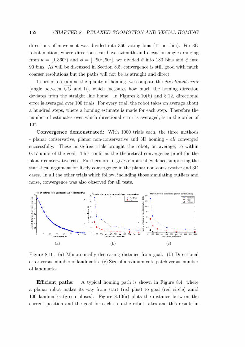
152 CHAPTER 8. RELAXED EGOMOTION AND VISUAL HOMING
directions of movement was divided into 360 voting bins (1◦ per bin). For 3D
robot motion, where directions can have azimuth and elevation angles ranging
from θ = [0, 360◦) and φ = [−90◦, 90◦], we divided θ into 180 bins and φ into
90 bins. As will be discussed in Section 8.5, convergence is still good with much
coarser resolutions but the paths will not be as straight and direct.
In order to examine the quality of homing, we compute the directional error
(angle between−→CG and h), which measures how much the homing direction
deviates from the straight line home. In Figures 8.10(b) and 8.12, directional
error is averaged over 100 trials. For every trial, the robot takes on average about
a hundred steps, where a homing estimate is made for each step. Therefore the
number of estimates over which directional error is averaged, is in the order of
104.
Convergence demonstrated: With 1000 trials each, the three methods
- planar conservative, planar non-conservative and 3D homing - all converged
successfully. These noise-free trials brought the robot, on average, to within
0.17 units of the goal. This confirms the theoretical convergence proof for the
planar conservative case. Furthermore, it gives empirical evidence supporting the
statistical argument for likely convergence in the planar non-conservative and 3D
cases. In all the other trials which follow, including those simulating outliers and
noise, convergence was also observed for all tests.
(a) (b)
0 100 200 300 400 500 600 700 800 900 10000
20
40
60
80
100
120
140
Number of landmarks
Nu
m o
f m
axim
um
vo
te b
ins (
ou
t o
f 3
60
)
Maximum vote patch size (planar, conservative)
maximum
mean
minimum
(c)
Figure 8.10: (a) Monotonically decreasing distance from goal. (b) Directional
error versus number of landmarks. (c) Size of maximum vote patch versus number
of landmarks.
Efficient paths: A typical homing path is shown in Figure 8.4, where
a planar robot makes its way from start (red plus) to goal (red circle) amid
100 landmarks (green pluses). Figure 8.10(a) plots the distance between the
current position and the goal for each step the robot takes and this results in

8.4. EXPERIMENTS AND RESULTS 153
a monotonically decreasing graph that drops to zero. The distance decreases
exponentially due to the non-uniform step size resulting from the proportional
control law used to vary step size.
Number of Landmarks: Figure 8.10(b) shows the effects of increasing the
number of landmarks on the directional error for the case of conservative, planar
homing. The smaller the directional error is, the closer the robot’s path is to the
straight line path to the goal. The mean error drops to less than 5◦ with more
than 300 points. Also shown is the maximum error, which is the maximum over
all steps for every one of the 100 trials. Even with as few as 50 points, the homing
vector, h, is always less than 68◦ from−→CG. Therefore, the robot always heads in
a direction that brings it closer to the goal. Since this is so, convergence on the
goal is certain.
Guaranteed convergence (planar, conservative): Figure 8.10(c) shows,
for the same experiment, the size of the patch (connected set) of bins with max-
imum votes. In the case of 50 landmark points, these bins form a patch that is,
at its largest, about 130◦ wide and−→CG must lie within this patch. The algo-
rithm takes h to be the average of all directions with the maximum vote, which
is roughly in the middle of this patch. Therefore,−→CG is less than 90◦ from h.
(In fact the same will hold for any patch that is less than 180◦ wide, refer Figure
8.11(a).) This is in accordance with the corresponding largest directional error
observed for 50 points, which is about 65◦ (Figure 8.10(b)). This occurs when−→CG is just at the border of the 130◦ wide patch.
For the case of a 100 landmarks or more, an even stronger condition for
convergence is met. As discussed earlier, as long as the maximum angle between
two directions in Dres is less than 90◦, every direction in Dres will be less than
90◦ from−→CG (illustrated in Figure 8.11(b)). From Figure 8.10(c), for 100 points
or more, the size of the maximum vote patch (corresponding to the size of Dres)
is always less than 90◦, and the above statement is verified by observing that the
maximum directional error (Figure 8.10(a)) is also always less than 90◦. This
implies both decreasing distance to the goal and successful convergence. The
stricter condition is useful in practice - for example, if the selected h is blocked
by an obstacle, every other direction in set Dres is a possible alternative that still
guarantees taking the robot closer to home.
Outliers: Under increasing proportions of outliers, successful convergence
was still observed for every trial. Figures 8.12(a-c) show performance under
increasing probability of random outliers in the data. The histograms show the
directional error from ∼ 104 homing estimates from 100 trials. 100 landmarks
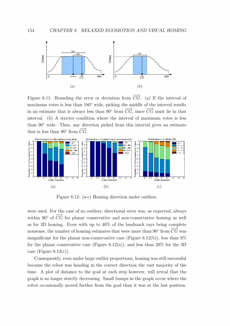
154 CHAPTER 8. RELAXED EGOMOTION AND VISUAL HOMING
(a) (b)
Figure 8.11: Bounding the error or deviation from−→CG. (a) If the interval of
maximum votes is less than 180◦ wide, picking the middle of the interval results
in an estimate that is always less than 90◦ from−→CG, since
−→CG must lie in that
interval. (b) A stricter condition where the interval of maximum votes is less
than 90◦ wide. Then, any direction picked from this interval gives an estimate
that is less than 90◦ from−→CG.
(a) (b) (c)
Figure 8.12: (a-c) Homing direction under outliers.
were used. For the case of no outliers, directional error was, as expected, always
within 90◦ of−→CG for planar conservative and non-conservative homing as well
as for 3D homing. Even with up to 40% of the landmark rays being complete
nonsense, the number of homing estimates that were more than 90◦ from−→CG was
insignificant for the planar non-conservative case (Figure 8.12(b)), less than 8%
for the planar conservative case (Figure 8.12(a)), and less than 20% for the 3D
case (Figure 8.12(c)).
Consequently, even under large outlier proportions, homing was still successful
because the robot was heading in the correct direction the vast majority of the
time. A plot of distance to the goal at each step however, will reveal that the
graph is no longer strictly decreasing. Small bumps in the graph occur where the
robot occasionally moved further from the goal than it was at the last position.

8.4. EXPERIMENTS AND RESULTS 155
Note that we used 100 landmarks for the 3D case as well even though the space
of possible homing directions is greatly increased. Using more landmarks would
further improve the performance of the 3D case.
Gaussian noise: Successful convergence was observed in all trials involving
increasing Gaussian noise. Figures 8.13(a-c) illustrate the performance as the
Gaussian noise standard deviation is varied from 0◦ to 9◦. Performance degrades
gracefully with noise but the proportion of homing vectors with directional error
greater than 90◦ is once again insufficient to prevent convergence. The non-
conservative planar method once again performs better than the conservative
planar method. Large Gaussian noise similarly causes the robot to oscillate about
the final goal.
(a) (b) (c)
Figure 8.13: (a-c) Homing direction under Gaussian noise.
Planar conservative vs. non-conservative: In experiments under outliers
and Gaussian noise, the planar non-conservative case outperformed the planar
conservative case in the sense that the homing direction deviated less from−→CG
(convergence was still observed in all the experiments conducted, but the paths
are less direct if homing direction deviates more from−→CG).
Although the conservative case is theoretically guaranteed to converge in the
noise free case, that guarantee comes at the cost of throwing away all constraints
that are not certain to be correct. In the process, many constraints which are
perfectly fine are thrown away as well.
Conversely, voting was robust to the incorrect constraints arising in the non-
conservative case. Since correct constraints dominate in number, these form a
robust peak in the vote space which requires large numbers of incorrect constraints
voting in consistency with each other, to perturb from its place. However, the
incorrect constraints are quite random and do not generally vote to a consistent
peak at all; and the ‘missed’ RC regions also tend to be small, so the total effect
on the performance of the non-conservative case is quite minimal.

156 CHAPTER 8. RELAXED EGOMOTION AND VISUAL HOMING
8.4.2 Real experiments
Grid trials
A camera captured omnidirectional images of some environment at every 10 cm
within a 1 m x 1 m grid. With some point on the grid as the home position, the
homing direction was calculated at every other point on the grid. The result is
summarized in a vector-field representation where each vector is the direction a
robot would move in if it was at that point in the field. By taking each point
on the grid in turn to be the home position, we can examine how the algorithm
performs in that environment for all combinations of start and goal positions
(marked with a ‘+’) within the grid.
All experiments on the planar conservative and planar non-conservative algo-
rithms were successful4. Figure 8.14 shows sample results from the three different
environments. Landmarks were SIFT features [145] matched between current and
goal images with code from [143].
The high-resolution (3840 x 1024) Ladybug camera [187] captured images of
a room (Figure 8.14(a)) and an office cubicle (b). Figures 8.14(c-d) are results for
the room using conservative and non-conservative algorithms respectively. Room
images were taken with the camera 0.85 m above the ground. This is necessary
for the conservative method, which requires landmarks both above and below the
image horizon. (In contrast, cubicle images were taken with the camera lying
on the floor and were unsuitable for the conservative algorithm since everything
below the horizon is featureless ground.)
Both conservative and non-conservative methods homed successfully in Fig-
ures 8.14(c-d). Since the conservative method discards many constraints, the
homing direction deviated further from−→CG, compared to the non-conservative
method which gave more direct homing paths. Nevertheless, it is clear that a
robot placed anywhere within the grid will follow the vectors and eventually
reach the goal position.
Figure 8.14(e) demonstrates successful homing in the cubicle environment
using the non-conservative method. We also tested the algorithm on a low-
resolution (360 x 143) outdoor image set supplied by authors of [276, 223]. Figure
8.14(f) is an example image from the set and 8.14(g) is a sample result. Inter-
estingly, the low-resolution outdoor images gave smoother vector fields than the
high-resolution, indoor ones. We believe this is due to a more even distribution of
4We leave real image experiments on 3D homing for future work.

8.4. EXPERIMENTS AND RESULTS 157
(a) (b)
(c) (d) (e)
(f) (g)
Figure 8.14: Grid trial experiments. (a) High-resolution panorama taken in a
room with an elevated camera and (b) taken in a cubicle with camera on the
floor. (c-d) Grid trials for room, comparing conservative and non-conservative
methods. (e) Grid trial result for the cubicle. (f) Low-resolution panorama taken
outdoors. (g) Grid trial result outdoors.

158 CHAPTER 8. RELAXED EGOMOTION AND VISUAL HOMING
landmarks outdoors, whereas indoors, features tend to be denser in some areas of
the image but are very sparse in other areas, leading to a bias in some directions.
However, convergence is unaffected and homing paths remain fairly straight.
Robot trials
(a) (b)
Figure 8.15: Robot trial experiments. (a) Robot’s view in the atrium experiment
from the upward-pointing fish-eye camera. The rim of the image corresponds to
the horizon of the world. (b) Robot in the office experiment.
A holonomic wheeled robot [42] homed in various environments including an
office and a building atrium. The robot performed local homing multiple times
to move along a chain of goal positions (simplest instance of the topological maps
mentioned in Section 8.1) in order to get from one part of the environment to
another. Images of the world were captured at each intermediate goal position
and stored in the map. This was done using an Omnitech Robotics fish-eye lens
camera [183], which was mounted pointing upwards, giving views such as Figure
8.15(a), where the image rim corresponds to the horizon.
The robot retrieves from memory the image corresponding to the next inter-
mediate goal position that it needs to get to, compares that with its current view
of the world, and uses the homing algorithms to drive there. After arriving, the
next image is then retrieved from the map and the procedure is repeated until
the final destination is reached.

8.5. DISCUSSION 159
This is illustrated in Figure 8.15(b), which shows an experiment where the
intermediate goal positions are marked with white squares5. The robot performs
long range homing by visiting these intermediate goal positions in turn until it
arrives at its final destination.
In these experiments, homing was successful to within the order of a few
centimeters, in the presence of mismatched landmarks, moving objects (leading
to bad landmark points) and illumination changes. For supplementary videos,
refer Appendix A.
8.5 Discussion
Robustness to outliers: Existing methods (see review in Section 3.2, page 52)
often assume that a correct correspondence has been found between landmarks
seen in the goal and current positions. However, if some of these landmarks have
moved, are moving, were occluded, or were erroneously matched - i.e. outliers
are present in the data - there is often no provision to ensure successful homing.
In methods such as [131, 140, 23, 9], a series of vectors, {M1, M2 · · ·MN}, are
typically derived from landmark bearings by some rule, and the average direction
is taken as the homing vector, Mres = M1 + M2 + · · ·+ MN . Unfortunately, this
average is sensitive to outliers which can potentially cause the homing vector to
point in any random direction. Conversely, the robust voting framework used in
our methods were demonstrated in experiments to be very resistant to significant
outlier and noise contamination.
Provable convergence. Homing is not provably successful in most of the
cited local homing methods. The work of Argyros et al. [9] showed successful
homing through extensive simulations. Loizou and Kumar [140] provided the first
planar homing algorithm with a proof of convergence. Our work differentiates
itself from Loizou and Kumar by proposing provably convergent algorithms for the
more general case where the relative rotation between current and goal positions
need not be known (compass-free), and where the landmarks need not lie on the
same plane as the robot.
Are there sufficient landmarks? More landmarks lead to more direct
homing paths. However, Observation 8.1 suggests that homing is successful as
long as homing directions are consistently less than 90◦ from−→CG. Computer
5The white squares were placed there so that the reader has an idea of where the intermediate
goal positions are. They were not used for homing by the robot and indeed, the robot does not
even see them since they are outside the FOV of the upward-pointing camera.

160 CHAPTER 8. RELAXED EGOMOTION AND VISUAL HOMING
vision methods such as SIFT matching [145] can typically find and match thou-
sands of feature points for some reasonable distance between the two views. A
small subset (a few hundred) of these should be more than enough since we earlier
saw that homing can work with even as few as 50 landmarks (Figure 8.10(b)).
Note that our method should work in the subcase of a robot being very close
to a blank wall where approximately half the space contains no or little land-
marks. This is because the goal position will lie in the half of the space that does
contain landmarks (it could not lie inside the blank wall). The homing direction
is sufficiently constrained to drive the robot in the general direction of the goal
and hence away from the wall, and subsequently the situation improves as the
robot moves further from the blank wall. In some circumstances however, there
may be the degenerate case of very few landmarks such that motion is not ade-
quately constrained. In such a case, we suggest falling back on methods such as
Argyros et al. [9], which work with a minimum of 3 landmarks.
Speed: A C++ implementation of our algorithm runs in 35 msec (28 fps)
on a Linux OS, Pentium4, 3GHz, 512Mb RAM machine (∼200 landmarks). The
bottleneck in the current system comes from the SIFT matching module which
takes several seconds to compute. However, real-time SIFT implementations (for
example, on a GPU [268]) do exist. Alternatively, faster feature tracking methods
such as KLT are also possible.
Poor Image Resolutions: The trials with low-resolution (360 x 143 pix-
els) outdoor images demonstrate that the algorithm works well even with poor
image resolutions. This is in agreement with the results of the simulations under
increasing Gaussian noise. The image noise in most cameras is generally in the
order of a couple of pixels (typically less than a degree), which is far less than the
amounts of Gaussian noise used in the simulations (up to 9◦). Therefore, what
these large noise trials do in fact simulate is the degradation of accuracy caused
by using very coarse image resolutions causing uncertainty in the landmark ray.
Voting Resolution: A large range of voting resolutions (not to be confused
with image resolution) can be used. Lower voting resolutions could achieve even
greater speeds without affecting convergence (it will, however, lead to a less direct
path home). In general, reducing voting resolution by a small amount leads to
little degradation in performance but an appreciable increase in processing speed,
especially for the case of 3D homing (order N2 increase in speed).
In fact, Observation 8.1 suggests that very coarse voting resolutions can be
used without affecting convergence. As an extreme example, for homing on the
plane, the conditions of Observation 8.1 are satisfied even with as few as 4 voting

8.6. CONCLUSION 161
bins (90◦ per bin), if h is the center of the bin and conservative voting was used.
The homing vector is then at most 45◦ from−→CG. Such a minimalist version of
the method is well-suited for small, resource limited robots.
Although convergence is unaffected, overly coarse resolutions will lead to the
robot taking a less than direct path, although that path would still be one where
the distance between the goal and the current robot position is a decreasing
function with each move that the robot makes.
Flexible Probability Maps: Whilst our experiments (and most existing
methods) obtained a single homing vector, the voting table is in fact a weighted
map of likely directions for homing. This leads to a flexible and natural framework
for incorporating additional navigational constraints such as obstacle avoidance,
kinematic constraints (in non-holonomic robots), centering behaviour and path
optimality planning. For example, directions blocked by obstacles can be aug-
mented with negative votes so that the robot is discouraged from moving in that
direction.
8.6 Conclusion
In summary, we have investigated the usefulness of relaxed egomotion estimates.
In particular, we considered relaxed translation estimates, which can be applied
to the problem of visual homing. We introduced weak constraints on camera
translation and proposed novel methods for robust homing that work in both
planar and 3D robots. Theoretical convergence guarantees can be shown for
the planar case (conservative method), whilst the planar non-conservative and
3D methods were shown by extensive simulation to converge empirically. The
method is fast, flexible and performed well in real and simulated experiments.


Chapter 9
Conclusion
9.1 Summary of Findings
One of the central ideas investigated in this work was how large FOV vision may
aid the task of egomotion estimation. To answer this question, we sought to
investigate those geometrical features of large FOV cameras which are not found
in small FOV devices. This, we hoped, would enable us to determine explicitly
what may be achieved with large FOV vision that cannot be achieved (or is harder
to achieve) with small FOV cameras.
We focused our attention on one such geometrical feature, that is, the antipo-
dal point. We showed that the geometry of antipodal points may be exploited
to decouple translation and rotation, leading to novel constraints on egomotion
under both differential and discrete camera motions. For the case of differen-
tial motion, antipodal point constraints represent a new way of decoupling the
camera translation and rotation. Furthermore, under the more general scenario
of discrete camera motion, antipodal points lead to the only known method for
decoupling motion and rendering a generally nonlinear or bilinear problem, linear.
Motion decoupling reduces the dimensionality of the problem, as it means
that translation and rotation may be found independently of each other i.e. the
5-dimensional problem is broken up into two smaller-dimensional ones. This is
important for the design of robust egomotion estimation methods, as it simplifies
the problem and leads to improvements in accuracy and efficiency. Standard
robust algorithms (e.g. RANSAC) based on the decoupled motion constraints
showed improved performance, whilst methods that were not as attractive for
solving higher dimensional problems (e.g. Hough-like voting) could now be used.
Experiments involving simulations and real images showed that the robust
163

164 CHAPTER 9. CONCLUSION
algorithms based on both our differential and discrete antipodal point constraints
performed competitively with the state-of-the-art. Overall, our algorithms showed
better robustness to large outlier proportions. Furthermore, they demonstrated
reduced run-time under increasing outlier proportions and those algorithms based
on Hough-voting in particular, performed in constant-time.
These results are important because they demonstrate a lesser known ad-
vantage of large FOV vision. Whilst it was previously well-known that a large
FOV improves the accuracy and stability of egomotion recovery methods (Section
3.1.4, page 43), here, we also demonstrated how large FOV vision may simplify
the task through motion decoupling, resulting in more efficient algorithms for
fast and robust egomotion recovery1.
Secondary to our main contributions on egomotion estimation was our work
on some applications that rely on knowledge of egomotion, such as the novel
structure-from-motion algorithm discussed in Chapter 7. We also proposed novel
algorithms for visual homing, and demonstrated that approximate or ‘relaxed’
egomotion measures can also be useful for certain applications, whilst being much
easier and faster to compute.
9.2 Future Work
9.2.1 Non-Central Cameras
The use of antipodal points requires a central or single viewpoint, large FOV
camera. If the camera is not single viewpoint, then the results of this thesis are
no longer applicable. An example of such a camera is shown in Figure 9.1, which
depicts the schematic of a multi-camera rig which has four individual camera
centres. This then, is motivation for extending the ideas of this thesis beyond
single viewpoint cameras to the more general case of non-central camera systems.
A first step in this direction may perhaps be found in the work of Hu and
Cheong [106], which formulates, under the differential motion assumption, equa-
tions for so-called ‘matching rays’ in a dual-camera rig (the construction of which,
is essentially similar to Figure 9.1, except that it consists of two cameras only).
However, in order to simplify the derived equations, Hu and Cheong then as-
sumed that the separation between the two cameras in the rig was negligible.
1Another example of a larger FOV resulting in faster motion estimation may be found in the
work of Hartley and Kahl [90], where the speed with which their branch-and-bound strategy
arrived at the optimal solution is significantly influenced by the size of the camera FOV.
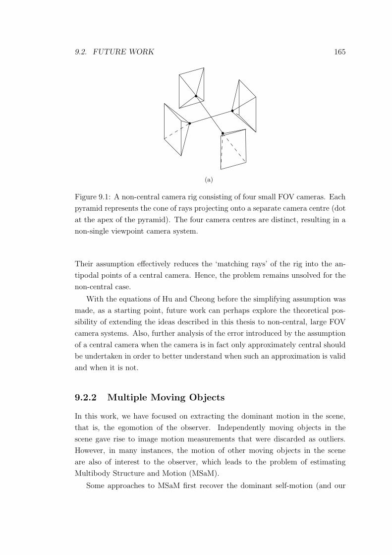
9.2. FUTURE WORK 165
(a)
Figure 9.1: A non-central camera rig consisting of four small FOV cameras. Each
pyramid represents the cone of rays projecting onto a separate camera centre (dot
at the apex of the pyramid). The four camera centres are distinct, resulting in a
non-single viewpoint camera system.
Their assumption effectively reduces the ‘matching rays’ of the rig into the an-
tipodal points of a central camera. Hence, the problem remains unsolved for the
non-central case.
With the equations of Hu and Cheong before the simplifying assumption was
made, as a starting point, future work can perhaps explore the theoretical pos-
sibility of extending the ideas described in this thesis to non-central, large FOV
camera systems. Also, further analysis of the error introduced by the assumption
of a central camera when the camera is in fact only approximately central should
be undertaken in order to better understand when such an approximation is valid
and when it is not.
9.2.2 Multiple Moving Objects
In this work, we have focused on extracting the dominant motion in the scene,
that is, the egomotion of the observer. Independently moving objects in the
scene gave rise to image motion measurements that were discarded as outliers.
However, in many instances, the motion of other moving objects in the scene
are also of interest to the observer, which leads to the problem of estimating
Multibody Structure and Motion (MSaM).
Some approaches to MSaM first recover the dominant self-motion (and our

166 CHAPTER 9. CONCLUSION
algorithms may be used for this first stage) before recovering the motions of other
objects in the scene [239, 205]. Other methods however, attempt to simultane-
ously segment and estimate all motion groups in a scene [254, 253, 134, 231, 195].
It would be interesting to investigate the possibility of extending the work of
this thesis to the problem of estimating multiple motions. Whilst we know that
a large FOV benefits self-motion recovery, we leave the question of whether large
FOV vision can also benefit the estimation of multiple motions, to future work.
9.2.3 Implementation of a Real-time Egomotion Recovery
System
This thesis focused on developing the theoretical basis for a number of novel
egomotion estimation algorithms. Although implementations of these algorithms
have been validated experimentally, going further to develop a practical, real-time
egomotion recovery system is non-trivial.
The current form of the algorithms are by no means the most efficient or
the fastest way of solving the task. Migrating from the predominantly Matlab
implementations to programs written in C is one obvious way of speeding up the
algorithms. We also advocate using parallel processing hardware (see the next
section) to realize further speedups.
9.2.4 Parallel Algorithms
A recurring theme in this thesis was the use of 2D Hough-reminiscent voting in
some of the algorithms presented. As noted previously, Hough-voting is highly
suitable for implementation on parallel processors. In comparison, the standard
solutions to the problem (e.g. 5-point and RANSAC) are fundamentally sequential
in nature, and attempting to implement these on parallel processors would see
only limited increases in speed.
As the computer industry undergoes a paradigm shift from increasing the
number of transistors in a single processor chip to increasing the number of
processors in a system, we believe that further work on parallel algorithms for
egomotion recovery should be done in order to take advantage of the massively
multi-core processors that are likely to become standard in the near future.
Parallel implementations of some of the algorithms described in this work, as
well as of the optical flow or point correspondence stage, could potentially form
the basis of a practical, real-time egomotion recovery system.

9.3. CONCLUSION 167
9.3 Conclusion
This thesis is a step toward faster and more robust egomotion recovery in complex,
noisy and outlier-prone, real-world scenes - scenes which humans and animals
appear to navigate and operate in, so effortlessly. In light of this, we were inspired
by the characteristics of eye and brain design in biology, such as the large FOV
vision possessed by many creatures, the spherical retina common to nearly all
sighted animals, and the fundamentally parallel architecture of neural systems.
Thus inspired, we investigated the geometry of large FOV cameras and of
image spheres, leading to the introduction of a number of constraints on egomo-
tion. Algorithms that utilized these constraints were proposed, including several
parallel, voting-based algorithms. The performance and advantages of these were
then demonstrated through both real and simulated experiments.
We hope that the ideas proposed in this work will stimulate further research
and progress in egomotion estimation, eventuating, some day, in stable and robust
technologies that find ubiquitous applications in our cars, homes and workplaces.


Appendix A
Supplementary Videos
Supplementary videos are available from the CD included with this thesis. Al-
ternatively, they are downloadable from the author’s website as a single file:
http://users.rsise.anu.edu.au/∼johnlim/
The folder “videos for chapter 6 experiments” show the experiments on real
image sequences for the lune+voting and GC+voting differential egomotion al-
gorithms. The estimate errors in Figures 6.8 and 6.9 of Chapter 6 are for the
experiments shown in these videos.
Meanwhile, the folder “videos for chapter 7 experiments” demonstrates the re-
sults for the real image experiments conducted on the discrete motion algorithms
proposed in Chapter 7 (cross reference results of Figure 7.8).
Videos showing robot homing in an office environment and in a larger atrium
environment using the algorithms proposed in Chapter 8 are found in the folder
“videos for chapter 8 experiments”.
Publications relevant to this thesis are also included for the reader’s conve-
nience.
169


Bibliography
[1] E. Adelson and J. Bergen. Spatiotemporal energy models for the perception
of motion. Journal of the Optical Society of America A, 2:284–299, 1985.
[2] G. Adiv. Determining three-dimensional motion and structure from optical
flow generated by several moving objects. IEEE Transactions on Pattern
Analysis and Machine Intelligence, 7:384–401, 1985.
[3] J. Aggarwal and N. Nandhakumar. On the computation of motion from
sequences of images: A review. Proceedings of the IEEE, 76(8):917–935,
August 1988.
[4] A. Agrawal and R. Chellappa. Ego-motion estimation and 3D model refine-
ment in scenes with varying illumination. In IEEE Workshop on Motion
and Video Computing,MOTIONS ’05, volume 2, pages 140–146, 2005.
[5] J. Aisbett. An iterated estimation of the motion parameters of a rigid
body from noisy displacement vectors. IEEE Trans. Pattern Analysis and
Machine Intelligence, 12(11):1092–1098, 1990.
[6] P. Anandan. A computational framework and an algorithm for the measure-
ment of visual motion. International Journal of Computer Vision, 2:283–
310, 1989.
[7] A. Angeli, D. Filliat, S. Doncieux, and J. Meyer. A fast and incremen-
tal method for loop-closure detection using bags of visual words. IEEE
Transactions On Robotics, Special Issue on Visual SLAM, 2008.
[8] M. E. Antone and S. Teller. Automatic recovery of relative camera rota-
tions for urban scenes. In Conference on Computer Vision and Pattern
Recognition, 2000.
171
172 BIBLIOGRAPHY
[9] A. Argyros, C. Bekris, S. Orphanoudakis, and L. Kavraki. Robot homing
by exploiting panoramic vision. Journal of Autonomous Robots, 19(1):7–25,
2005.
[10] X. Armangue, H. Araujo, and J. Salvi. A review on egomotion by means of
differential epipolar geometry applied to the movement of a mobile robot.
Pattern Recognition, 36(12):2927–2944, December 2003.
[11] M. Atiquzzaman. Multiresolution Hough transform - an efficient method of
detecting patterns in images. IEEE Transactions on Pattern Analysis and
Machine Intelligence, 14(11):1090–1095, 1992.
[12] A. Bab-Hadiashar and D. Suter. Robust optic flow computation. Interna-
tional Journal of Computer Vision, 29(1):59–77, 1998.
[13] P. Baker, A. S. Ogale, and C. Fermuller. The Argus eye: A new tool for
robotics. IEEE Robotics and Automation Magazine, 11(4), 2004.
[14] S. Baker and I. Matthews. Lucas-Kanade 20 years on: A unifying frame-
work. International Journal of Computer Vision, 56(3):221–255, 2004.
[15] D. Ballard and O. Kimball. Rigid body motion from depth and optical flow.
Computer Vision, Graphics and Image Processing, 22:95–115, 1984.
[16] A. Barron and M. V. Srinivasan. Visual regulation of ground speed and
headwind compensation in freely flying honey bees (Apis mellifera L.). Jour-
nal of Experimental Biology, 209:978–984, 2006.
[17] J. L. Barron, D. J. Fleet, and S. S. Beauchemin. Performance of optical
flow techniques. International Journal of Computer Vision, 12(1):43–77,
1994.
[18] A. Basu and S. Licardie. Alternative models for fish-eye lenses. Pattern
Recognition Letters, 16(4):433–441, 1995.
[19] A. Baumberg. Reliable feature matching across widely separated views. In
Conference on Computer Vision and Pattern Recognition, pages 774–781,
2000.
[20] L. Baumela, L. Agapito, I. Reid, and P. Bustos. Motion estimation us-
ing the differential epipolar equation. In International Conf. on Pattern
Recognition, volume 3, pages 840–843, 2000.

BIBLIOGRAPHY 173
[21] H. Bay, A. Ess, T. Tuytelaars, and L. V. Gool. SURF: Speeded up robust
features. Computer Vision and Image Understanding (CVIU), 110(3):346–
359, 2008.
[22] J. Bazin, C. Demonceaux, P. Vasseur, and I. Kweon. Motion estimation
by decoupling rotation and translation in catadioptric vision. Computer
Vision and Image Understanding, 2009.
[23] K. Bekris, A. Argyros, and L. Kavraki. Angle-based methods for mobile
robot navigation: Reaching the entire plane. In Proc. Int. Conf. on Robotics
and Automation, pages 2373–2378, 2004.
[24] R. Benosman and S. Kang (editors). Panoramic Vision. MIT Springer,
2001.
[25] R. Benosman, T. Maniere, and J. Devars. A generic camera model and
calibration method for conventional, wide-angle and fish-eye lenses. In Pro-
ceedings of the 13th International Conference on Pattern Recognition, pages
161–165, 1996.
[26] Y. Boykov, O. Veksler, and R. Zabih. Fast approximate energy minimisa-
tion via graph cuts. IEEE Transactions on Pattern Analysis and Machine
Intelligence, 29:1222–1239, 2001.
[27] J. Bresenham. Algorithm for computer control of a digital plotters. IBM
Systems Journal, 4(1):25–30, 1965.
[28] T. Brodsky, C. Fermuller, and Y. Aloimonos. Directions of motion fields are
hardly ever ambiguous. International Journal of Computer Vision, 26:5–24,
1998.
[29] T. J. Broida and R. Chellappa. Estimation of object motion parameters
from noisy images. IEEE Trans. Pattern Analysis and Machine Intelligence,
8(1):90–99, January 1986.
[30] T. Brox, A. Bruhn, N. Papenberg, and J. Weickert. High accuracy optical
flow estimation based on a theory for warping. In European Conference on
Computer Vision, pages 25–36, 2004.
[31] A. R. Bruss and B. K. Horn. Passive navigation. Computer Vision, Graphics
and Image Processing, 21:3–20, 1983.

174 BIBLIOGRAPHY
[32] B. Buxton and H. Buxton. Computation of optic flow from the motion of
edge features in image sequences. Image and Vision Computing, 2(2):59–75,
1984.
[33] T. Camus. Method for real time correlation of stereo images. In US Patent
6516087, 2003.
[34] L. Carrol. Through the Looking-Glass, and What Alice Found There.
Macmillan, 1871.
[35] B. Cartwright and T. Collett. Landmark learning in bees. Journal of
Comparative Physiology A, 151(4):521–543, 1983.
[36] J. Chahl and M. Srinivasan. Reflective surfaces for panoramic imaging.
Applied Optics, 36(31):8275–8285, 1997.
[37] H. Chen and P. Meer. Robust regression with projection based M-
estimators. In IEEE Int. Conference on Computer Vision, pages 878–885,
2003.
[38] A. Chiuso, R. Brockett, and S. Soatto. Optimal structure from motion:
local ambiguities and global estimates. International Journal on Computer
Vision, 39(3):195–228, 2000.
[39] W. Chojnacki, M. J. Brooks, A. van den Hengel, and D. Gawley. Revisiting
Hartley’s normalised eight-point algorithm. IEEE Transactions on Pattern
Analysis and Machine Intelligence, 9(25):1172–1177, 2003.
[40] C. Chu and E. Delp. Estimating displacement vector from an image se-
quence. Journal of the Optical Society of America A, 6:871–878, 1989.
[41] C. Clifford, K. Langley, and D. Fleet. Centre-frequency adaptive IIR tem-
poral filters for phase-based image velocity estimation. International Con-
ference on Image Processing and Applications, pages 173–178, 1995.
[42] L. Cole and N. Barnes. Insect inspired three dimensional centering. In Proc.
Australasian Conf. on Robotics and Automation, 2008.
[43] D. Comaniciu and P. Meer. Mean shift: A robust approach toward fea-
ture space analysis. IEEE Transactions on Pattern Analysis and Machine
Intelligence, 24(5):603–619, 2002.

BIBLIOGRAPHY 175
[44] H. Coxeter. Introduction to Geometry. New York: Wiley, 1969.
[45] M. Cummins and P. Newman. Highly scalable appearance-only SLAM
FAB-MAP 2.0. In Robotics Science and Systems (RSS), Seattle, USA,
June 2009.
[46] L. da Vinci. The Notebooks of Leonardo da Vinci. circa 1500 AD. (edited
J.P. Richter, 1880).
[47] K. Daniilidis. Fixation simplifies 3D motion estimation. Computer Vision
and Image Understanding, 68:158–169, 1997.
[48] K. Daniilidis and H.-H. Nagel. The coupling of rotation and translation in
motion estimation of planar surfaces. In Proc. IEEE Conf. on Computer
Vision and Pattern Recognition, pages 188–193, June 1993.
[49] K. Daniilidis and M. Spetsakis. Visual navigation: from biological systems
to unmanned ground vehicles, chapter : Understanding noise sensitivity in
structure from motion, pages 61–88. Hillsdale: Lawrence Erlbaum, 1997.
(editor: Y. Aloimonos).
[50] A. Davison. Real-time simultaneous localisation and mapping with a single
camera. In Proc. International Conference on Computer Vision, 2003.
[51] R. den Hollander and A. Hanjalic. A combined RANSAC-Hough transform
algorithm for fundamental matrix estimation. In Proc. 18th British Machine
Vision Conference, 2007.
[52] S. Derrien and K. Konolige. Approximating a single viewpoint in panoramic
imaging devices. In Proc. IEEE Workshop Omnidirectional Vision, pages
85–90, 2000.
[53] Draganfly Innovations Inc. <http://www.draganfly.com>, 2009.
[54] R. O. Duda and P. E. Hart. Pattern Classification and Scene Analysis. New
York: Wiley, 1973.
[55] H. Esch, S. Zhang, M. Srinivasan, and J. Tautz. Honeybee dances commu-
nicate distances measured by optic flow. Nature, 411:581–583, 2001.
[56] Euclid. Optics. circa 300 BC. (The Arabic version of Euclid’s Optics,
translated and edited by Elaheh Kheirandish, Springer, 1999).

176 BIBLIOGRAPHY
[57] O. Faugeras, Q. Luong, and T. Papadopoulo. The Geometry of Multiple
Images. MIT Press, 2001.
[58] O. Faugeras, F. Lustman, and G. Toscani. Motion and structure from point
and line matches. In Proc. International Conference on Computer Vision,
June 1987.
[59] O. Faugeras and S. Maybank. Motion from point matches: Multiplicity of
solutions. International Journal of Computer Vision, 4(3):225–246, 1990.
[60] C. Fermuller. Passive navigation as a pattern recognition problem. Inter-
national Journal of Computer Vision, 14(2):147–158, 1995.
[61] C. Fermuller and Y. Aloimonos. The role of fixation in visual motion anayl-
sis. International Journal of Computer Vision, 11:165–186, 1993.
[62] C. Fermuller and Y. Aloimonos. Direct perception of three-dimensional
motion from patterns of visual motion. Science, 270:1973–1976, 1995.
[63] C. Fermuller and Y. Aloimonos. Qualitative egomotion. International Jour-
nal of Computer Vision, 15:7–29, 1995.
[64] C. Fermuller and Y. Aloimonos. Ambiguity in structure from motion:
Sphere versus plane. International Journal of Computer Vision, 28:137–
154, 1998.
[65] M. Fischler and R. Bolles. Random sample consensus: A paradigm for
model fitting with applications to image analysis and automated cartogra-
phy. Comm. of the ACM, 24:381–395, 1981.
[66] D. Fleet. Measurement of Image Velocity. Kluwer Academic Press, 1992.
[67] D. Fleet and A. Jepson. Computation of component image velocity from
local phase information. International Journal of Computer Vision, 5:77–
104, 1990.
[68] M. Franz and H. Mallot. Biomimetic robot navigation. Biomimetic Robots,
Robotics and Autonomous Systems, 30(1):133–153, 2000.
[69] M. Franz, B. Scholkopf, H. Mallot, and H. Bulthoff. Learning view graphs
for robot navigation. Autonomous Robots, 5(1):111–125, 1998.

BIBLIOGRAPHY 177
[70] M. Franz, B. Scholkopf, H. Mallot, and H. Bulthoff. Where did I take that
snapshot? Scene-based homing by image matching. Biological Cybernetics,
79(3):191–202, 1998.
[71] F. Fraundorfer, C. Engels, and D. Nister. Topological mapping, localization
and navigation using image collections. In International Conference on
Intelligent Robots and Systems, 2007.
[72] A. Fusiello. Uncalibrated Euclidean reconstruction: A review. Image and
Vision Computing, 18:555–563, 2000.
[73] C. Geyer and K. Daniilidis. Catadioptric camera calibration. In Proc. Int.
Conf. on Computer Vision (ICCV), pages 398–404, 1999.
[74] C. Geyer and K. Daniilidis. Structure and motion from uncalibrated cata-
dioptric views. In IEEE Conf. Computer Vision and Pattern Recognition,
pages 279–286, Dec 2001.
[75] C. Geyer and K. Daniilidis. Paracatadioptric camera calibration. Pattern
Analysis and Machine Intelligence, 24(5):687–695, May 2002.
[76] J. Gluckman and S. Nayar. Ego-motion and omnidirectional cameras. In
Proc. Int’l Conf. Computer Vision, 1998.
[77] R. Goecke, A. Asthana, N. Pettersson, and L. Petersson. Visual vehicle
egomotion estimation using the Fourier-Mellin transform. In Proc. IEEE
Intelligent Vehicles Symposium, pages 450–455, June 2007.
[78] T. Goedeme, T. Tuytelaars, and L. V. Gool. Visual topological map build-
ing in self-similar environments. In Int. Conf. on Informatics in Control,
Automation and Robotics, 2006.
[79] N. Goncalves and H. Araujo. Estimating parameters of noncentral cata-
dioptric systems using bundle adjustment. Computer Vision and Image
Understanding, 113(1):11–28, 2009.
[80] A. Goshtasby, S. Gage, and J. Bartholic. A two-stage cross correlation ap-
proach to template matching. IEEE Trans. Pattern Analysis and Machine
Intelligence, 6(3):374–378, 1984.
178 BIBLIOGRAPHY
[81] S. Gourichon, J. Meyer, and P. Pirim. Using colored snapshots for short
range guidance in mobile robots. Int. J. Robot. Automation, 17:154–162,
2002.
[82] N. Grzywacz and A. Yuille. A model for the estimate of local velocity. In
Proc. European Conf. on Computer Vision, pages 331–335, 1990.
[83] N. Gupta and L. Kanal. Gradient based image motion estimation without
computing gradients. Int. J. Comput. Vision, 22(1):81–101, 1997.
[84] F. Hampel. Beyond location parameters: robust concepts and methods.
Bulletin of the Int. Statist. Inst., 46:375–382, 1975.
[85] C. Harris and M. Stephens. A combined corner and edge detector. In 4th
Alvey Vision Conference, pages 147–151, 1988.
[86] R. Hartley. Estimation of relative camera positions for uncalibrated cam-
eras. In Proc. European Conference on Computer Vision, 1992.
[87] R. Hartley. In defence of the 8-point algorithm. In Proceedings of the 5th
International Conference on Computer Vision, pages 1064–1070, 1995.
[88] R. Hartley, E. Hayman, L. de Agapito, and I. Reid. Camera calibration and
the search for infinity. In Proceedings of the IEEE International Conference
on Computer Vision, 1999.
[89] R. Hartley and F. Kahl. Global optimization through searching rotation
space and optimal estimation of the essential matrix. In Proc. International
Conference on Computer Vision, 2007.
[90] R. Hartley and F. Kahl. Global optimization through rotation space search.
International Journal of Computer Vision, 82(1):64–79, 2009.
[91] R. Hartley and F. Schaffalitzky. L∞ minimization in geometric reconstruc-
tion problems. In Proc. IEEE Conference on Computer Vision and Pattern
Recognition, pages 504–509, 2004.
[92] R. Hartley and P. Sturm. Triangulation. Computer Vision and Image
Understanding, 68(2):146–157, 1997.
[93] R. Hartley and A. Zisserman. Multiple View Geometry in Computer Vision.
Cambridge University Press, 2004.

BIBLIOGRAPHY 179
[94] D. Heeger. Optical flow using spatiotemporal filters. International Journal
of Computer Vision, 1:279–302, 1988.
[95] J. Heel. Direct estimation of structure and motion for multiple frames. In
Technical Report 1190, MIT AI Lab, 1989.
[96] J. Heel. Direct dynamic motion vision. In Proc. IEEE Conference on
Robotics and Automation, 1990.
[97] J. Heikkila and O. Silven. A four-step camera calibration procedure with
implicit image correction. In Proc. of IEEE Computer Vision and Pattern
Recognition, pages 1106–1112, 1997.
[98] H. Helmholtz. Handbuch der Physiologischen Optik. Leipzig: Voss, 1867.
(Treatise on Physiological Optics, translated by J.P.C. Southall, New York:
Dover, 1962).
[99] E. Hildreth. The computation of the velocity field. Proc. of the Royal
Society of London B, 221:189–220, 1984.
[100] E. Hildreth. Recovering heading for visually-guided navigation. Vision
Research, 32(6):1177–1192, 1992.
[101] J. Hong, X. Tan, B. Pinette, R. Weiss, and E. Riseman. Image-based
homing. IEEE Control Systems Magazine, 12:38–45, 1992.
[102] B. Horn and B. Schunck. Determining optical flow. Artificial Intelligence,
17:185–204, 1981.
[103] B. Horn and E. Weldon. Direct methods for recovering motion. Int. Journal
on Computer Vision, 2(1):51–76, 1988.
[104] P. Hough. Method and means for recognizing complex patterns. US Patent
3,069,654, December 1962.
[105] C. Hu and L. Cheong. Linear ego-motion recovery algorithm based on quasi-
parallax. In International Conference on Image Processing, pages 233–236,
2008.
[106] C. Hu and L. Cheong. Linear quasi-parallax SFM using laterally-placed
eyes. International Journal on Computer Vision, 84(1):21–39, 2009.
[107] P. Huber. Robust Statistics. Wiley, 2004.

180 BIBLIOGRAPHY
[108] S. Hutchinson, G. Hager, and P. Corke. A tutorial on visual servo control.
IEEE Trans. Robotics and Automation, 12(5):651–670, 1996.
[109] J. Illingworth and J. V. Kittler. The adaptive Hough transform. IEEE
Transactions on Pattern Analysis and Machine Intelligence, 9(5):690–698,
1987.
[110] J. Illingworth and J. V. Kittler. A survey of the Hough transform. Computer
Vision, Graphics and Image Processing, 44(1):87–116, 1988.
[111] Intel Open Source Computer Vision Library. available from:
<http://sourceforge.net/projects/opencv>, 2007.
[112] M. Irani, B. Rousso, and S. Peleg. Recovery of ego-motion using region
alignment. IEEE Transactions on Pattern Analysis and Machine Intelli-
gence, 19(3):268–272, 1997.
[113] B. Jahne. Motion determination in space-time images. In Proc. European
Conf. on Computer Vision, pages 161–173, 1990.
[114] A. Jepson and D. Heeger. Subspace methods for recovering rigid motion I:
algorithm and implementation. International Journal of Computer Vision,
7(2), 1992.
[115] A. Jepson and D. Heeger. Linear subspace methods for recovering transla-
tion direction. In Spatial Vision in Humans and Robots. Cambridge Uni-
versity Press, 1993.
[116] H. Jin, P. Favaro, and S. Soatto. Real-time 3-D motion and structure from
point features: a front end system for vision-based control and interaction.
In Proc. IEEE Intl. Conf. on Computer Vision and Pattern Recognition,
pages 778–779, 2000.
[117] F. Kahl. Multiple view geometry and the L∞-norm. In Proc. International
Conference on Computer Vision, pages 1002–1009, 2005.
[118] K. Kanatani. 3-D interpretation of optical flow by renormalization. Inter-
national Journal of Computer Vision, 11(3), 1992.
[119] K. Kanatani. Comparing optimal 3-D reconstruction for finite motion and
optical flow. Journal of Electronic Imaging, 12(3):478–488, 2003.

BIBLIOGRAPHY 181
[120] K. Kanatani, Y. Shimizu, N. Ohta, M. Brooks, W. Chojnacki, and
A. van den Hengel. Fundamental matrix from optical flow: optimal compu-
tation and reliability evaluation. Journal of Electronic Imaging, 9(2):194–
202, April 2000.
[121] S. Kang. Catadioptric self-calibration. In Proc. Computer Vision and Pat-
tern Recognition (CVPR), volume 1, pages 201–207, 2000.
[122] J. Kannala and S. Brandt. A generic camera model and calibration method
for conventional, wide-angle and fish-eye lenses. IEEE Transactions on
Pattern Analysis and Machine Intelligence, 28:1335–1340, 2006.
[123] S. Karabernou and F. Terranti. Real-time FPGA implementation of Hough
transform using gradient and CORDIC algorithm. Image and Vision Com-
puting, 23(11):1009–1017, 2005.
[124] J. Koenderink. The structure of images. Biological Cybernetics, 50:363–396,
1984.
[125] J. Koenderink and A. van Doorn. Invariant properties of the motion paral-
lax field due to the movement of rigid bodies relative to an observer. Optica
Acta, 22(9):773–791, 1975.
[126] J. Koenderink and A. van Doorn. Local structure of movement parallax of
the plane. Jour. of the Optical Society of America, 66:717–723, 1976.
[127] P. D. Kovesi. MATLAB and Octave Functions for Computer Vi-
sion and Image Processing, School of Computer Science & Soft-
ware Engineering, The University of Western Australia, available from:
<http://www.csse.uwa.edu.au/∼pk/research/matlabfns/>.
[128] B. Kuipers and Y. Byun. A robot exploration and mapping strategy
based on a semantic hierarchy of spatial representations. Robotics and
Autonomous Systems, 8:47–63, 1991.
[129] Z. Kukelova, M. Bujnak, and T. Pajdla. Polynomial eigenvalue solutions to
the 5-pt and 6-pt relative pose problems. In Proc. British Machine Vision
Conference (BMVC), 2008.
[130] R. Kumar, A. Tirumalai, and R. C. Jain. A non-linear optimization al-
gorithm for the estimation of structure and motion parameters. In Proc.

182 BIBLIOGRAPHY
IEEE Conf. on Computer Vision and Pattern Recognition, pages 136–143,
June 1989.
[131] D. Lambrinos, R. Moller, T. Labhart, R. Pfeifer, and R. Wehner. A mo-
bile robot employing insect strategies for navigation. Biomimetic Robots,
Robotics and Autonomous Systems, 30:39–64, 2000.
[132] D. Lawton and W. Carter. Qualitative spatial understanding and the con-
trol of mobile robots. In IEEE Conf. on Decision and Control, pages 1493–
1497, 1990.
[133] J. Lee, B. Wood, and T. Newman. Very fast ellipse detection using GPU-
based RHT. In International Conference on Pattern Recognition, 2008.
[134] H. Li. Two-view motion segmentation from linear programming relaxation.
In IEEE Conf. Computer Vision and Pattern Recognition (CVPR), 2007.
[135] H. Li. Consensus set maximization with guaranteed global optimality for
robust geometry estimation. In Proc. International Conf. Computer Vision,
2009.
[136] H. Li and R. Hartley. Five-point motion estimation made easy. In 18th
International Conference on Pattern Recognition (ICPR’06), pages 630–
633, 2006.
[137] Z. Li, B. Yao, and F. Tong. A linear generalized Hough transform and
its parallel implementation. In IEEE Conference on Computer Vision and
Pattern Recognition, 1991.
[138] W. Lin, G. Tan, and L. Cheong. When discrete meets differential- assess-
ing the stability of structure from small motion. International Journal of
Computer Vision, June 2009.
[139] T. Lindeberg. Scale-space theory: A basic tool for analysing structures at
different scales. Journal of Applied Statistics, 21(2):224–270, 1994.
[140] S. Loizou and V. Kumar. Biologically inspired bearing-only navigation and
tracking. In IEEE Conf. on Decision and Control, 2007.
[141] H. Longuet-Higgins. A computer algorithm for reconstruction of a scene
from two projections. Nature, 293:133–135, 1981.

BIBLIOGRAPHY 183
[142] H. C. Longuet-Higgins and K. Prazdny. The interpretation of a moving reti-
nal image. Proceedings of the Royal Society of London. Series B, Biological
Sciences, 208(1173):385–397, 1980.
[143] D. Lowe. Sift implementation available from (accessed 2009):
<http://www.cs.ubc.ca/∼lowe/keypoints/>.
[144] D. Lowe. Object recognition from local scale-invariant features. In Inter-
national Conference on Computer Vision, pages 1150–1157, 1999.
[145] D. Lowe. Distinctive image features from scale-invariant keypoints. Inter-
national Journal of Computer Vision, 60(2):91–110, 2004.
[146] B. D. Lucas and T. Kanade. An iterative image registration technique with
an application to stereo vision. In Proceedings of Imaging Understanding
Workshop, pages 121–130, 1981.
[147] Q.-T. Luong, R. Deriche, O. Faugeras, and T. Papadopoulo. On determin-
ing the fundamental matrix: Analysis of different methods and experimen-
tal results. Technical Report RR-1894, INRIA, 1993.
[148] Y. Ma, J. Kosecka, and S. Sastry. Motion recovery from image sequences:
Discrete viewpoint vs. differential viewpoint. In European Conference on
Computer Vision, 1998.
[149] Y. Ma, J. Kosecka, and S. Sastry. Linear differential algorithm for motion
recovery: a geometric approach. International Journal on Computer Vision,
36(1), 2000.
[150] W. Maclean, A. Jepson, and R. Frecker. Recovery of egomotion and seg-
mentation of independent object motion using the EM algorithm. In British
Machine Vision Conference, pages 13–16, 1994.
[151] M. J. Magee and J. K. Aggarwal. Determining vanishing points from per-
spective images. Computer Vision, Graphics and Image Processing, 26:256–
267, 1984.
[152] M. Mainberger, A. Bruhn, and J. Weickert. Is dense optic flow useful to
compute the fundamental matrix? In Proc. of the 5th Int. Conf. on Image
Analysis and Recognition, pages 630–639, 2008.

184 BIBLIOGRAPHY
[153] A. Makadia and K. Daniilidis. Rotation estimation from spherical images.
IEEE Transactions on Pattern Analysis and Machine Intelligence, 28:1170–
1175, 2006.
[154] A. Makadia, C. Geyer, S. Sastry, and K. Daniilidis. Radon-based structure
from motion without correspondences. In IEEE Conference on Computer
Vision and Pattern Recognition, June 2005.
[155] J. Matas and O. Chum. Randomized RANSAC with td,d test. Image and
Vision Computing, 22(10):837–842, 2004.
[156] J. Matas and O. Chum. Optimal randomized RANSAC. IEEE Transactions
on Pattern Analysis and Machine Intelligence, 30(8):1472–1482, 2008.
[157] J. Matas, O. Chum, M. Urban, and T. Pajdla. Robust wide baseline stereo
from maximally stable extremal regions. In British Machine Vision Con-
ference, pages 384–393, 2002.
[158] L. Matthies, R. Szeliski, and T. Kanade. Kalman filter-based algorithm for
estimating depth from image sequences. In Proc. Conference on Computer
Vision and Pattern Recognition, June 1988.
[159] S. Maybank. The angular velocity associated with the optical flow field
arising from motion through a rigid environment. Proceedings of the Royal
Society of London, 410:317–326, 1985.
[160] S. J. Maybank and O. Faugeras. A theory of self-calibration of a moving
camera. International Journal of Computer Vision, 8:123–151, 1992.
[161] B. Micusik and T. Pajdla. Estimation of omnidirectional camera model
from epipolar geometry. In Proc. Computer Vision and Pattern Recognition
(CVPR), pages 485–490, 2003.
[162] B. Micusik and T. Pajdla. Autocalibration and 3D reconstruction with non-
central catadioptric cameras. In Conf. on Computer Vision and Pattern
Recognition (CVPR), 2004.
[163] B. Micusik and T. Pajdla. Structure from motion with wide circular field
of view cameras. IEEE Transactions on Pattern Analysis and Machine
Intelligence, 28(7):1135–1149, 2006.

BIBLIOGRAPHY 185
[164] K. Mikolajczyk and C. Schmid. An affine invariant interest point detector.
In European Conference on Computer Vision, pages 128–142, 2002.
[165] R. Moller. Insect visual homing strategies in a robot with analog process-
ing. Biological Cybernetics: special issue in Navigation in Biological and
Artificial Systems, 83(3):231–243, 2000.
[166] H. Moravec. Rover visual obstacle avoidance. In International Joint Con-
ference on Artificial Intelligence, pages 785–789, 1981.
[167] E. Mouragnon, M. Lhuillier, M. Dhome, F. Dekeyser, and P. Sayd. Generic
and real time structure from motion. In Proceedings of the 18th British
Machine Vision Conference, 2007.
[168] M. Muhlich and R. Mester. The role of total least squares in motion anal-
ysis. In Proc. European Conf. Computer Vision, 1998.
[169] D. Murray. Recovering range using virtual multicamera stereo. Computer
Vision and Image Understanding, 61(2):285–291, 1995.
[170] H.-H. Nagel. On the estimation of optic flow: Relations between different
approaches and some new results. Artificial Intelligence, 33:299–324, 1987.
[171] S. Nayar. Catadioptric omnidirectional camera. In Proc. Computer Vision
and Pattern Recognition (CVPR), pages 482–488, 1997.
[172] S. Negahdaripour and B. Horn. Direct passive navigation. IEEE Transac-
tions on Pattern Analysis and Machine Intelligence, 9(1):168–176, 1987.
[173] S. Negahdaripour and B. Horn. A direct method for locating the focus of
expansion. Computer Vision, Graphics and Image Processing, 46:303–326,
1989.
[174] S. Negahdaripour and C. H. Yu. A generalized brightness change model for
computing optical flow. In Proc. Int’l Conf. Computer Vision, pages 2–11,
1993.
[175] R. Nelson and J. Aloimonos. Finding motion parameters from spherical
flow fields (or the advantages of having eyes in the back of your head).
Biological Cybernetics, 58:261–273, 1988.

186 BIBLIOGRAPHY
[176] J. Neumann. Computer Vision in the Space of Light Rays: Plenoptic Video
Geometry and Polydioptric Camera Design. 2003. PhD Thesis.
[177] J. Neumann, C. Fermuller, and Y. Aloimonos. Eyes from eyes: New cameras
for structure from motion. In IEEE Workshop on Omnidirectional Vision
2002, pages 19–26, June 2002.
[178] J. Neumann, C. Fermuller, and Y. Aloimonos. Polydioptric camera de-
sign and 3D motion estimation. In IEEE Computer Society Conference on
Computer Vision and Pattern Recognition, pages 294–301, 2003.
[179] D. Nister. An efficient solution to the five-point relative pose problem. In
Proc. Conference on Computer Vision and Pattern Recognition, 2003.
[180] D. Nister. Preemptive RANSAC for live structure and motion estimation.
In Proc. IEEE International Conference on Computer Vision (ICCV 2003),
pages 199–206, April 2003.
[181] D. Nister. An efficient solution to the five-point relative pose problem.
IEEE Transactions on Pattern Analysis and Machine Intelligence (PAMI),
pages 756–770, 2004.
[182] M. Ogata and T. Sato. Motion detection model with two-stages: spa-
tiotemporal filtering and feature matching. Journal of the Optical Society
of America A, 9:377–387, 1992.
[183] Omnitech Robotics. <http://www.omnitech.com/>, 2009.
[184] T. Pajdla, T. Svoboda, and V. Hlavac. Panoramic Vision, chapter : Epipo-
lar Geometry of Central Panoramic Catadioptric Cameras, pages 73–102.
Springer, 2001. (editors: R. Benosman and S.B. Kang).
[185] J. Patel and A. N. Choudhary. Parallel Architectures and Parallel Algo-
rithms for Integrated Vision Systems. Kluwer Academic Pub, 1990.
[186] R. Pless. Using many cameras as one. In Conf. on Computer Vision and
Pattern Recognition (CVPR), 2003.
[187] Point Grey Research. <http://www.ptgrey.com>, 2007.
[188] M. Pollefeys, R. Koch, and L. V. Gool. Self-calibration and metric re-
construction in spite of varying and unknown internal camera parameters.

BIBLIOGRAPHY 187
In Proceedings of the IEEE International Conference on Computer Vision,
pages 90–95, 1998.
[189] I. Powell. Panoramic fish-eye imaging system. In US Patent 5631778, 1997.
[190] K. Prazdny. Egomotion and relative depth map from optical flow. Biological
Cybernetics, 36:87–102, 1980.
[191] K. Prazdny. On the information in optical flows. Computer Graphics and
Image Processing, 22:239–259, 1983.
[192] J. Prince and E. McVeigh. Motion estimation from tagged MR image se-
quences. IEEE Trans. on Medical Imaging, 11:238–249, 1992.
[193] M. Pupilli and A. Calway. Real-time camera tracking using a particle filter.
In Proc. British Machine Vision Conference (BMVC’05), pages 519–528,
September 2005.
[194] G. Qian and R. Chellappa. Structure from motion using sequential Monte
Carlo methods. In Proceedings of Eighth IEEE International Conference
on Computer Vision, pages 614–621, July 2001.
[195] N. Quadrianto, T. Caetano, J. Lim, and D. Schuurmans. Convex relax-
ation of mixture regression with efficient algorithms. In Advances in Neural
Information Processing Systems (NIPS), 2009.
[196] L. Quan and R. Mohr. Determining perspective structures using hierarchi-
cal Hough transform. Pattern Recognition Letters, 9(4):279–286, 1989.
[197] R. Raguram, J. M. Frahm, and M. Pollefeys. A comparative analysis of
RANSAC techniques leading to adaptive real-time random sample consen-
sus. In European Conference on Computer Vision, pages 500–513, 2008.
[198] S. Ramalingam, P. Sturm, and S. Lodha. Towards complete generic cam-
era calibration. In Conf. on Computer Vision and Pattern Recognition
(CVPR), pages 1093–1098, 2005.
[199] J. Rieger and D. Lawton. Processing differential image motion. Jour. of
the Optical Society of America A, 2(2):354–359, 1985.
[200] J. W. Roach and J. K. Aggarwal. Determining the movement of objects
from a sequence of images. IEEE Transactions on Pattern Analysis and
Machine Intelligence, 2(6):55–62, 1980.

188 BIBLIOGRAPHY
[201] C. Rother and S. Carlsson. Linear multi-view reconstruction and camera
recovery. In Proc. International Conf. Computer Vision, pages 42–50, 2001.
[202] P. Rousseeuw. Least median of squares regression. Jour. Amer. Statist.
Assoc, 79:871–880, 1984.
[203] J. Salvi, X. Armangue, and J. Batlle. A comparative review of cam-
era calibrating methods with accuracy evaluation. Pattern Recognition,
35(7):1617–1635, July 2002.
[204] R. Satzoda, S. Suchitra, and T. Srikanthan. Parallelizing the Hough trans-
form computation. Signal Processing Letters, 15:297–300, 2008.
[205] K. Schindler and D. Suter. Two-view multibody structure-and-motion with
outliers through model selection. IEEE Trans. Pattern Analysis and Ma-
chine Intelligence, 28(6):983–995, 2006.
[206] C. Schmid and R. Mohr. Local grayvalue invariants for image retrieval.
IEEE Trans. on Pattern Analysis and Machine Intelligence, 19(5):530–534,
1997.
[207] B. Schunck. Image flow: Fundamentals and future research. In Proc. Int.
Conf. on Pattern Recognition, pages 560–571, 1985.
[208] O. Shakernia, R. Vidal, and S. Sastry. Omnidirectional vision-based ego-
motion estimation from backprojection flows. In Proc. IEEE Workshop
Omnidirectional Vision, 2003.
[209] J. Shi and C. Tomasi. Good features to track. In IEEE Conference on
Computer Vision and Pattern Recognition, pages 593–600, 1994.
[210] J. Shufelt. Performance evaluation and analysis of vanishing point detection
techniques. IEEE Transactions on Pattern Analysis and Machine Intelli-
gence, 21(3):282–288, 1999.
[211] C. Silva and J. Santos-Victor. Direct egomotion estimation. In Proc. 13th
International Conference on Pattern Recognition, volume 1, pages 702–706,
1996.
[212] C. Silva and J. Santos-Victor. Robust egomotion estimation from the nor-
mal flow using search subspaces. IEEE Transactions on Pattern Analysis
and Machine Intelligence, 19(9):1026–1034, 1997.

BIBLIOGRAPHY 189
[213] E. Simoncelli and E. Adelson. Computing optical flow distributions us-
ing spatio-temporal filters. Technical report, MIT Media Lab Vision and
Modeling, Technical Report, 1991.
[214] P. Sobey and M. V. Srinivasan. Measurement of optical flow by a generalized
gradient scheme. Journal of the Optical Society of America A, 8:1488–1498,
1991.
[215] M. Srinivasan. Generalized gradient schemes for the measurement of two-
dimensional image motion. Biological Cybernetics, 63(6):421–431, 1990.
[216] M. Srinivasan, J. Chahl, K. Weber, S. Venkatesh, M. Nagle, and S. Zhang.
Robot navigation inspired by principles of insect vision. Robotics and Au-
tonomous Systems, 26:203–216, 1999.
[217] M. Srinivasan, M. Lehrer, W. Kirchner, and S. Zhang. Range perception
through apparent image speed in freely-flying honeybees. Visual Neuro-
science, 6:519–535, 1991.
[218] M. Srinivasan, S. Zhang, M. Lehrer, and T. Collett. Honeybee naviga-
tion enroute to the goal: visual flight control and odometry. Journal of
Experimental Biology, 199:237–244, 1996.
[219] G. Stein, O. Mano, and A. Shashua. A robust method for computing vehicle
ego-motion. In IEEE Intelligent Vehicles Symposium (IV2000), October
2000.
[220] G. P. Stein and A. Shashua. Model-based brightness constraints: On direct
estimation of structure and motion. IEEE Transactions on Pattern Analysis
and Machine Intelligence, 22(9):992–1015, 2000.
[221] H. Stewenius, C. Engels, and D. Nister. An efficient minimal solution for in-
finitesimal camera motion. In Conference on Computer Vision and Pattern
Recognition, 2007.
[222] P. Sturm and S. Ramalingam. A generic camera calibration concept. In
European Conf. on Computer Vision (ECCV), 2004.
[223] W. Sturzl and J. Zeil. Depth, contrast and view-based homing in outdoor
scenes. Biological Cybernetics, 96:519–531, 2007.

190 BIBLIOGRAPHY
[224] J. Suhr, H. Jung, K. Bae, and J. Kim. Outlier rejection for cameras on
intelligent vehicles. Pattern Recognition Letters, 29(6):828–840, April 2008.
[225] M. Sutton, W. Wolters, W. Peters, and S. McNiell. Determination of dis-
placements using an improved digital correlation method. Image and Vision
Computing, 1(3):133–139, 1983.
[226] T. Svoboda and T. Pajdla. Epipolar geometry for central catadioptric
cameras. International Journal of Computer Vision, 49(1):23–37, 2002.
[227] T. Svoboda, T. Pajdla, and V. Hlavac. Motion estimation using central
panoramic cameras. In IEEE International Conf. on Intelligent Vehicles,
pages 335–340, June 1998.
[228] R. Szeliski and S. B. Kang. Recovering 3D shape and motion from image
streams using non-linear least squares. In Proceedings IEEE Conference on
Computer Vision and Pattern Recognition, pages 752–753, June 1993.
[229] M. Taalebinezhaad. Direct recovery of motion and shape in the general
case by fixation. IEEE Trans. Pattern Analysis and Machine Intelligence,
14:847–853, 1992.
[230] S. Tagzout, K. Achourb, and O. Djekouneb. Hough transform algorithm
for FPGA implementation. Signal Processing, 81(6):1295–1301, 2001.
[231] N. Thakoor and J. Gao. Branch-and-bound hypothesis selection for two-
view multiple structure and motion segmentation. In IEEE Conf. Computer
Vision and Pattern Recognition (CVPR), 2008.
[232] T. Thanh, H. Nagahara, R. Sagawa, Y. Mukaigawa, M. Yachida, and
Y. Yagi. Robust and real-time rotation estimation of compound omnidi-
rectional sensor. In Proc. IEEE International Conference on Robotics and
Automation, April 2007.
[233] I. Thomas and E. Simoncelli. Linear structure from motion. Technical
report, IRCS, University of Pennsylvania, 1994.
[234] S. Thrun, W. Burgard, and D. Fox. Probabilistic Robotics. MIT Press,
2005.
BIBLIOGRAPHY 191
[235] T. Tian, C. Tomasi, and D. Heeger. Comparison of approaches to egomo-
tion computation. In IEEE Conference on Computer Vision and Pattern
Recognition, pages 315–320, 1996.
[236] E. Tola, V. Lepetit, and P. Fua. A fast local descriptor for dense matching.
In Conference on Computer Vision and Pattern Recognition, 2008.
[237] C. Tomasi and J. Shi. Direction of heading from image deformations. In
Conference on Computer Vision and Pattern Recognition, pages 422–427,
1993.
[238] A. Torii and A. Imiya. The randomized-Hough-transform-based method for
great-circle detection on a sphere. Pattern Recognition Letters, 28(10):1186–
1192, 2007.
[239] P. Torr. Geometric motion segmentation and model selection. Philosophical
Trans. of the Royal Society of London, 356(1740):1321–1340, 1998.
[240] P. Torr and A. Zisserman. Robust computation and parametrization of
multiple view relations. In Proceedings of the Sixth International Conference
on Computer Vision, pages 727–732, 1998.
[241] P. Torr and A. Zisserman. MLESAC: A new robust estimator with applica-
tion to estimating image geometry. Journal of Computer Vision and Image
Understanding, 78(1):138–156, 2000.
[242] B. Triggs. Autocalibration and the absolute quadric. In Proceedings of
the IEEE Conference on Computer Vision and Pattern Recognition, pages
609–614, 1997.
[243] B. Triggs. Differential matching constraints. In Proc. International Conf.
Computer Vision, 1999.
[244] B. Triggs. Plane + parallax, tensors and factorization. In Proc. European
Conf. Computer Vision, pages 522–538, 2000.
[245] B. Triggs, P. F. McLauchlan, R. I. Hartley, and A. W. Fitzgibbon. Bundle
adjustment - a modern synthesis. In Vision Algorithms ’99, pages 298–372,
1999.

192 BIBLIOGRAPHY
[246] R. Tsai. An efficient and accurate camera calibration technique for 3D
machine vision. In Proceedings of IEEE Conference on Computer Vision
and Pattern Recognition, pages 364–374, 1986.
[247] R. Tsai and T. Huang. Uniqueness and estimation of 3-D motion parameters
of rigid bodies with curved surfaces. IEEE Trans. Pattern Analysis and
Machine Intelligence, 6:13–27, 1984.
[248] T. Tuytelaars and L. V. Gool. Wide baseline stereo based on local, affinely
invariant regions. In British Machine Vision Conference, pages 412–422,
2000.
[249] O. Tuzel, R. Subbarao, and P. Meer. Simultaneous multiple 3D motion
estimation via mode finding on Lie groups. In 10th IEEE Int. Conference
on Computer Vision, pages 18–25, 2005.
[250] S. Ullman. The interpretation of structure from motion. Proceedings of the
Royal Society of London, pages 405–426, 1979.
[251] A. Vardy and R. Moller. Biologically plausible visual homing methods based
on optical flow techniques. Connection Science, 17(1):47–89, 2005.
[252] A. Verri and T. Poggio. Motion field and optical flow: Qualitative prop-
erties. IEEE Transactions on Pattern Analysis and Machine Intelligence,
11(5):490–498, 1989.
[253] R. Vidal, Y. Ma, S. Soatto, and S. Sastry. Two-view multibody structure
from motion. International Journal on Computer Vision (IJCV), 68(1):7–
25, 2006.
[254] R. Vidal and S. Sastry. Optimal segmentation of dynamic scenes from two
perspective views. In IEEE Conf. Computer Vision and Pattern Recognition
(CVPR), 2003.
[255] T. Vieville and O. D. Faugeras. The first order expansion of motion equa-
tions in the uncalibrated case. Computer Vision and Image Understanding,
64(1):128–146, 1996.
[256] S. Segvic, G. Schweighofer, and A. Pinz. Influence of numerical conditioning
on the accuracy of relative orientation. In IEEE Conf. on Computer Vision
and Pattern Recognition, 2007.
BIBLIOGRAPHY 193
[257] N. Wade and S. Finger. The eye as an optical instrument: from camera
obscura to Helmholtz’s perspective. Perception, 30:1157–1177, 2001.
[258] A. Watson and A. Ahumada. Model of human visual motion sensing. Jour-
nal of the Optical Society of America A, 2:322–341, 1985.
[259] A. Waxman and S. Ullman. Surface structure and three-dimensional motion
from image flow kinematics. International Journal of Robotics Research,
4:72–94, 1985.
[260] J. Weber, J. Malik, S. Devadas, and P. Michel. Robust computation of
optical flow in a multi-scale differential framework. International Journal
of Computer Vision, 14:12–20, 1994.
[261] K. Weber, S. Venkatesh, and M. Srinivasan. Insect-inspired robotic homing.
Adaptive Behavior, 7(1):65–97, 1999.
[262] J. Weng, T. Huang, and N. Ahuja. Motion and structure from two perspec-
tive views: Algorithms, error analysis, and error estimation. IEEE Trans.
Pattern Analysis and Machine Intelligence, 11:451–476, 1989.
[263] C. Wheatstone. Contributions to the physiology of vision. Part the first: On
some remarkable, and hitherto unobserved, phenomena of binocular vision.
Phil. Trans. of the Royal Society of London, 128:371–394, 1838.
[264] A. Witkin. Scale-space filtering. In International Joint Conference on
Artificial Intelligence, pages 1019–1022, 1983.
[265] K. Wohn, J. Wu, and R. Brockett. A contour-based recovery of image flow:
Iterative transformation method. IEEE Trans. Pattern Anal. Mach. Intell.,
13(8):746–760, 1991.
[266] W. Wolfe, D. Mathis, C. Sklair, and M. Magee. The perspective view of 3
points. IEEE Transactions on Pattern Analysis and Machine Intelligence,
13, 1991.
[267] WowWee. <http://www.wowwee.com/en/support/flytech-dragonfly>,
2009.
[268] C. Wu. SiftGPU: A GPU Implementation of SIFT (accessed: 26 May 2009)
http://www.cs.unc.edu/∼ccwu/siftgpu/.

194 BIBLIOGRAPHY
[269] F. Wu, F. Duan, Z. Hu, and Y. Wu. A new linear algorithm for calibrat-
ing central catadioptric cameras. Pattern Recognition, 41(10):3166–3172,
October 2008.
[270] T. Xiang and L. Cheong. Understanding the behavior of SFM algorithms: a
geometric approach. International Journal on Computer Vision, 51(2):111–
137, 2003.
[271] L. Xu, E. Oja, and P. Kultanen. A new curve detection method: Random-
ized Hough transform. Pattern Recognition Letters, 11(5):331–338, 1990.
[272] B. L. Yen and T. S. Huang. Determining 3-D motion and structure of a
rigid body using the spherical projection. In Computer Vision, Graphics
and Image Processing, volume 21, pages 21–32, 1983.
[273] X. Ying and Z. Hu. Catadioptric camera calibration using geometric invari-
ants. Pattern Analysis and Machine Intelligence, 26(10):1260–1271, Octo-
ber 2004.
[274] X. Ying and H. Zha. Linear approaches to camera calibration from sphere
images or active intrinsic calibration using vanishing points. In Proc. Int.
Conf. on Computer Vision (ICCV), pages 596–603, 2005.
[275] X. Ying and H. Zha. Identical projective geometric properties of central
catadioptric line images and sphere images with applications to calibration.
Int. J. on Computer Vision (IJCV), 78(1):89–105, June 2008.
[276] J. Zeil, M. Hoffmann, and J. Chahl. Catchment areas of panoramic images
in outdoor scenes. Journal of the Optical Society of America A, 20(3):450–
469, 2003.
[277] Z. Zhang. Determining the epipolar geometry and its uncertainty: A review.
Technical Report RR-2927, INRIA, 1996.
[278] Z. Zhang. A flexible new technique for camera calibration. IEEE Transac-
tions on Pattern Analysis and Machine Intelligence, 22:1330–1334, 2000.
[279] Z. Zhang. Camera calibration. In Emerging Topics in Computer Vision,
pages 4–43. Prentice Hall, 2004. (editors: G. Medioni and S.B. Kang).

BIBLIOGRAPHY 195
[280] Z. Zhang, R. Deriche, O. Faugeras, and Q. Luong. A robust technique for
matching two uncalibrated images through the recovery of the unknown
epipolar geometry. Artificial Intelligence, 78:87–119, 1995.
[281] X. Zhuang, T. Huang, N. Ahuja, and R. Haralick. A simplified linear optic
flow motion algorithn. Computer Vision, Graphics, and Image Processing,
pages 334–344, 1988.
[282] J.-C. Zufferey, A. Klaptocz, A. Beyeler, J.-D. Nicoud, and D. Floreano. A
10-gram vision-based flying robot. Advanced Robotics, 21(14):1671–1684,
2007.