Embed Size (px)
Citation preview

MATHCAD Fundamentals and
Functions – Session III
EGN 1006 – Introduction to Engineering

MATHCAD
Data Analysis and Statistical AnalysisAnalysis

Statistical Functions
MATHCAD offers the capability to perform statistical analysis by a number of built-in functions that can be applied directly to the data contained in single or multi-dimensional arraysdimensional arrays
� mean(A) Mean or Average
� stdev(A) Standard Deviation
� var(A) Variance

Enter the following
Create a matrix A with 11 rows and 1 column. Enter the following values as shown then type:shown then type:
mean(A)=
stdev(A)=
var(A)=

Interpolation Functions
MATHCAD is capable of automatically interpolating data using several degrees of approximation
� linterp(Vx,Vy,p) Linear Interpolation
lspline(V ,V ) Linear Spline� lspline(Vx,Vy) Linear Spline
� pspline(Vx,Vy) Parabolic Spline
� cspline(Vx,Vy) Cubic Spline
� interp(Vs,Vx,Vy.p) General Interpolation from spline output
� corr(Vx1,Vx2) correlates two arrays for residuals

What is a spline?
The linear spline represents a set of line segments between the between the two adjacent
data points

Enter the following
Create an 11r,1c Matrix called “time” and enter the values shown.
Create an 11r,1c Matrix called “T” and enter the values shown
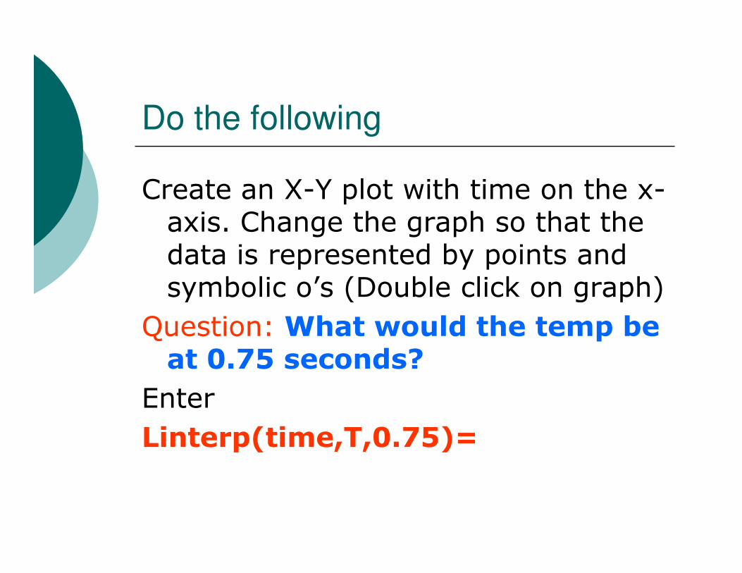
Do the following
Create an X-Y plot with time on the x-axis. Change the graph so that the data is represented by points and symbolic o’s (Double click on graph)symbolic o’s (Double click on graph)
Question: What would the temp be at 0.75 seconds?
Enter
Linterp(time,T,0.75)=
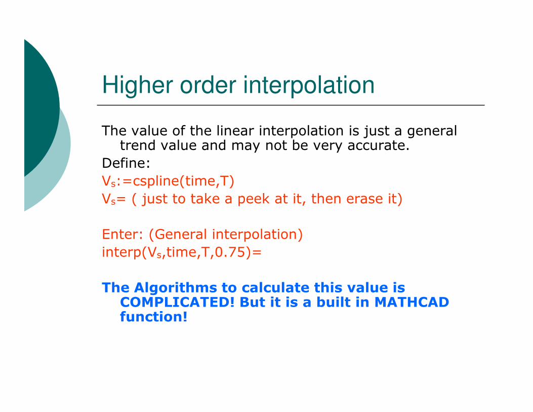
Higher order interpolation
The value of the linear interpolation is just a general trend value and may not be very accurate.
Define:
Vs:=cspline(time,T)
Vs= ( just to take a peek at it, then erase it)s
Enter: (General interpolation)
interp(Vs,time,T,0.75)=
The Algorithms to calculate this value is COMPLICATED! But it is a built in MATHCAD function!

Curve Fitting Functions
MATHCAD includes several functions that produce the coefficients for several curve models.
� intercept(Vx,Vy) linear y-intersection� intercept(Vx,Vy) linear y-intersection
� slope(Vx,Vy) linear slope
� linfit(Vx,Vy,f) generalized regression
Produces as many coefficients as required by the dimensions of the function f

Enter the following
Our time/temp graph may look straight but we cannot assume it is.
Define
b:=intercept(time,T)b:=intercept(time,T)
b=
m:=slope(time,T)
m=

Do the following
Let’s say we want to see the line of best fit! Copy and Paste the graph underneath all current work.
Enter the following ABOVE the pasted graph:
Note: The T(linear) uses BOTH a text subscript AND an index subscript). Also, notice that we are using the equation of a line y=mx+b

Do the following
Click on the “T” on the graph then hit the “comma” key on the keyboard. This keyboard. This will create another entry box. Enter in T(linear) then hit enter. You should see:

A general regression
First we must define a function ”f”. Create and define a function f(x) as a 3x1 matrix as shown. This matrix represents the equation of a parabola a+bx+cx2. Then define “a” using linfit command
Enter:a= These are the COEFFICIENTS in the
parabola equation
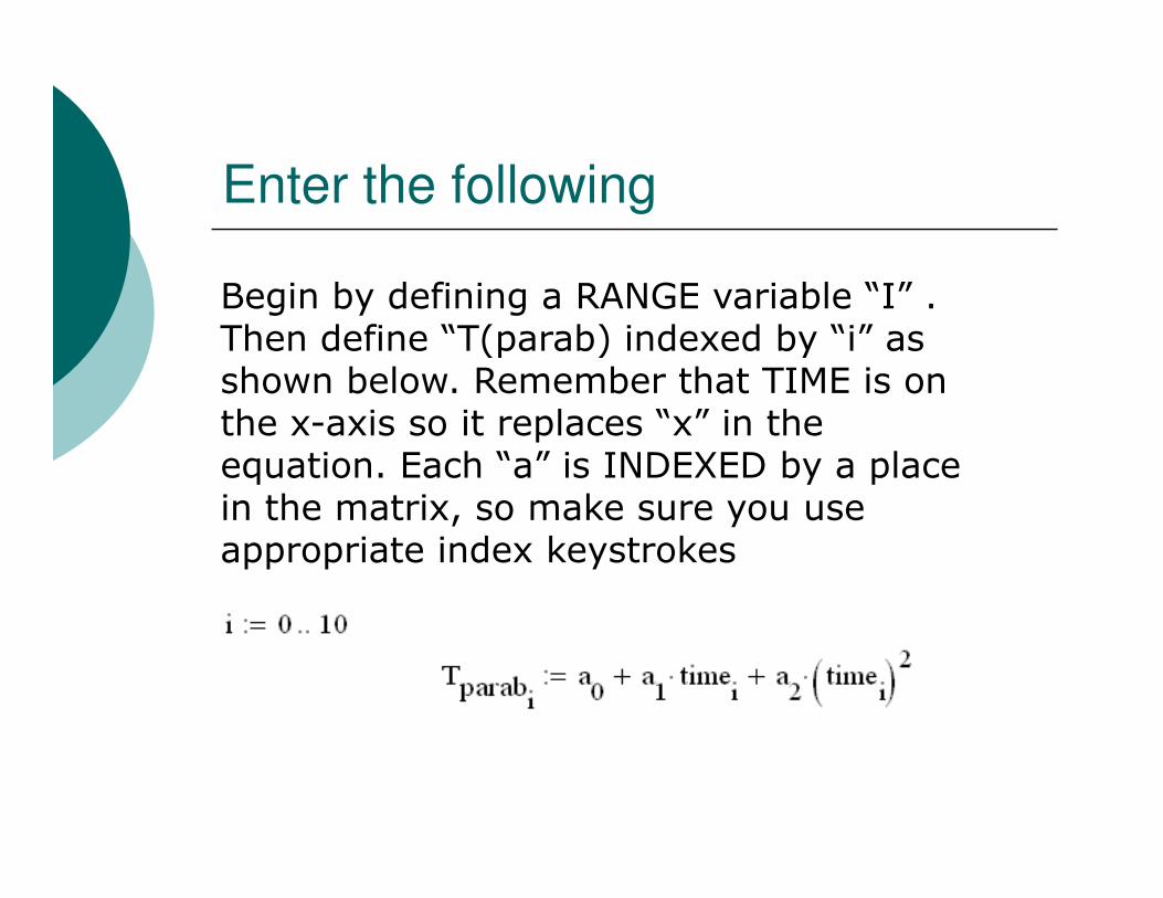
Enter the following
Begin by defining a RANGE variable “I” . Then define “T(parab) indexed by “i” as shown below. Remember that TIME is on the x-axis so it replaces “x” in the equation. Each “a” is INDEXED by a place equation. Each “a” is INDEXED by a place in the matrix, so make sure you use appropriate index keystrokes

Do the following
Click on the “T” on the graph and once again hit the comma key to insert a NEW line insert a NEW line on the graph, with this one being parabolic in nature. You should see:

How “CLOSE” is the data?
We now want to compare how the T(linear) and the T(parab) fit with the original data “T”.
Enter this below the graphEnter this below the graph
corr(Tlinear,T)=
corr(Tparab,T)=
You can easily see which one is a better fit as we desire to get a value close to ONE!
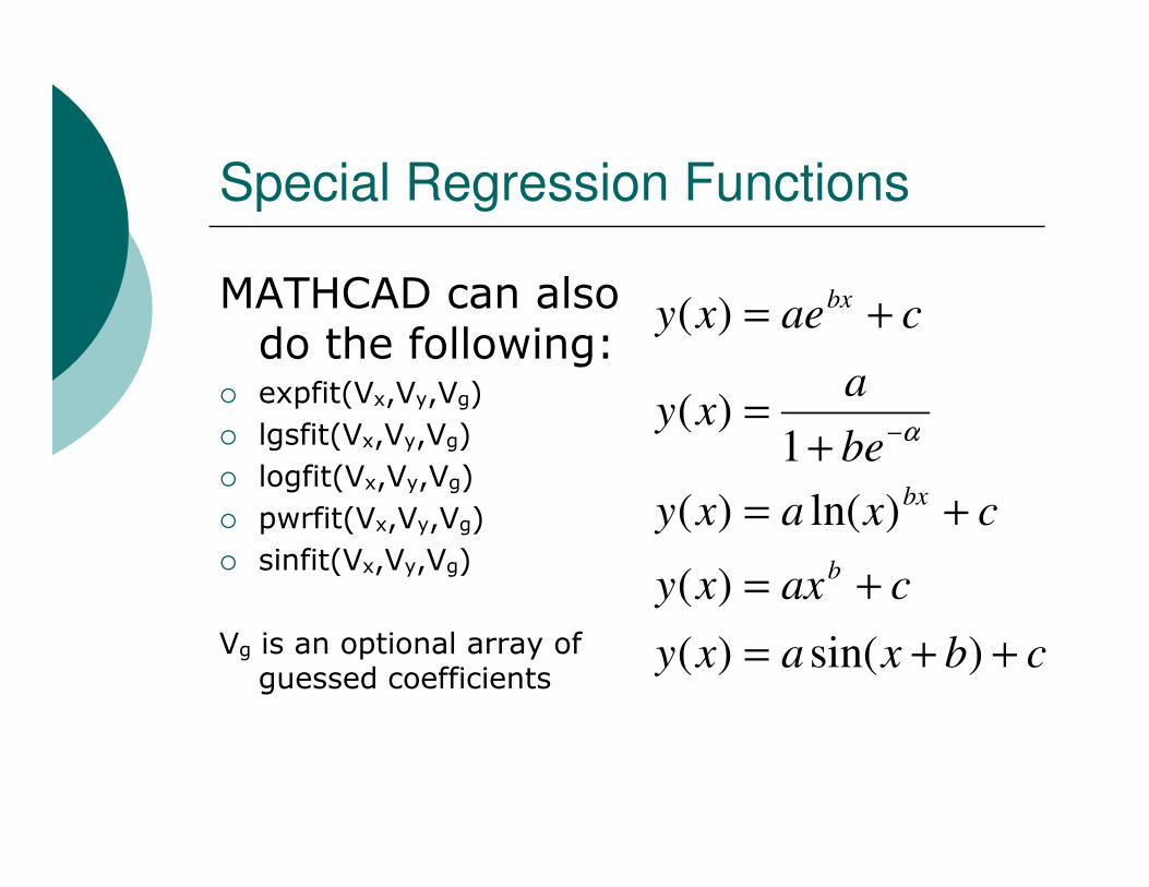
Special Regression Functions
MATHCAD can also do the following:
� expfit(Vx,Vy,Vg)
� lgsfit(Vx,Vy,Vg) be
axy
caexybx
+
=
+=
−
1)(
)(
α� lgsfit(Vx,Vy,Vg)
� logfit(Vx,Vy,Vg)
� pwrfit(Vx,Vy,Vg)
� sinfit(Vx,Vy,Vg)
Vg is an optional array of guessed coefficients
cbxaxy
caxxy
cxaxy
be
b
bx
++=
+=
+=
+−
)sin()(
)(
)ln()(
1α

Enter the following
First we will define a special array of guessed coefficients. Define Vg as a 3x1 matrix Vg as a 3x1 matrix as shown. The define “a” then enter a= to see the REAL coefficients. You should see:

Try this!
Using what you have already done,
REPEAT this entire process and do an EXPONENTIAL fit. Add the exponential curve on a second exponential curve on a second pasted graph and do a correlation between Texp and T
DO NOT LOOK AT THE NEXT SLIDE UNTIL TOLD!

YOU SHOULD SEE

You should see

Complete the following assignment