Economic and Financial Report 2004/01

Systemic Credit Risk in the Presence of Concentration

Federico Galizia Operations Directorate

European Investment Bank 100 Bd Konrad Adenauer

L-2950 Luxembourg Telephone : +352 4379 -1

f.galizia@eib.org JEL Classification codes:

E3 - Prices, Business Fluctuations, and Cycles

G3 - Corporate Finance and Governance

Notes

ECONOMIC AND FINANCIAL REPORTS are preliminary material circulated to stimulate discussion and critical comment. Quotation of material in the Reports should be cleared with the author or authors. The views expressed are those of the individual authors, and do not necessarily reflect the position of the EIB. Individual copies of the Reports may be obtained free of charge by writing to the above address. They are also available on-line from http://www.eib.org/efs/

1

Systemic Credit Risk in the Presence of

Concentration

Federico Galizia

Abstract

In a Black-Scholes-Merton model of single name default, instability could be seen as the level of volatility that would trigger default, everything else equal. At a portfolio level, for instance comprising all credit liabilities of the corporate sector, potential for instability could be measured by a credit portfolio loss distribution. For such a loss distribution, it should then be possible to define a level of volatility that would trigger instability, for instance by producing credit losses in excess of the aggregate capital of the banking system. This paper analyses the potential for instability in the Euro area by looking at both aggregate and name-level data for the corporate sector. Loss distributions are computed under plausible hypotheses for the underlying default, loss and correlation parameters, and our conclusion is that aggregate bank capital could cover losses at a very high confidence level; in other words, the likelihood of financial instability is negligible. However, we identify a sizable degree of concentration in the aggregate liabilities of Euro zone non-financial corporations. Significant concentration, even at investment grade, augments potential credit losses (measured as Credit Value at Risk) in a similar way to a substantial increase in the aggregate average default probability or the average asset return correlation. Further analysis is warranted in order to assess the level of volatility that could trigger default of a “concentrated exposure” and to better understand under which conditions this could lead to instability.

2

1. INTRODUTION: VOLATILITY VS INSTABILITY Dealing with the topic of Financial Instability is a task of daunting complexity. The few academic authors that have taken up the challenge (most notable in recent times are Charles Kindleberger and Hyman P. Minsky) have succeeded in devising an initial taxonomy of financial crises and their causes. However, most would agree that moving beyond classification into a tightly knit and consistent theory of Financial Instability is still work in progress. IMF’s twice-yearly issues of the Global Financial Stability Report “provide a regular assessment of global financial markets and identify potential system weakness that could lead to crises” (IMF 2003). Again, the focus is chiefly descriptive, enriched by in-depth analysis of various crisis episodes and related policy responses. Many studies posit a connection between episodes of high volatility in the prices of financial assets and episodes of financial instability. While “volatility, simply put refers to the degree to which prices vary over a certain length of time … Financial system instability is often linked to concerns about key financial institutions becoming illiquid or failing …” (IMF, 2003). The motivation of this paper is to explore a formal, however narrow, link between the related concepts of volatility and instability via the Black-Scholes-Merton model (BSM) of default, in the version popularised by Moody's|KMV (2003) and RiskMetrics (1997). In the BSM model, a company will default whenever the value of its assets falls below the nominal value of the liabilities. Everything else equal, an increase in asset volatility augments the likelihood of such an occurrence. The attractiveness of the BSM framework is that it features a discontinuity (i.e. a default) along a path of increasing volatility in asset returns. In a model of single name default, instability could be seen as the level of volatility that would trigger default, everything else equal. At an aggregate level, the joint process of default of a portfolio of names can be derived by their joint asset dynamics. Thus, if one thinks of systemic Financial Instability as entailing the joint default of a number of companies and banks, a BSM model of an economic system could represent a relevant “laboratory” test for systemic risk. Gray, Merton and Bodie (2003) have extended the BSM framework to a macroeconomic setup. While being more limited in a number of ways, our analysis differs in that we utilise explicitly the concept of a loss distribution and we study the implications of concentration on financial instability. A portfolio model is first and foremost a tool to quantify the likelihood of a given level of losses on a credit portfolio, over a definite time horizon. This measure is typically read off a loss distribution. If this portfolio is assembled at the level of a single bank, one can derive the loss distribution in order to assess the likelihood that the bank will remain solvent over the period, which is given by the probability of losses not exceeding the bank’s capital and reserves. The same concept can be applied at a macroeconomic level, for instance, taking aggregate loans from the financial sector to the corporate sector. The resulting loss distribution could be used to evaluate the solvency of the financial system as a whole, thus translating the general concept of systemic risk into a less general, but also more concrete concept of Financial Instability. While the analysis in Gray, Merton and Bodie (2003) encompasses all macroeconomic sectors and quantifies the risk of instability at a macroeconomic level, this paper explicitly models liabilities issued by the major corporates1 and banks in the Euro area. By computing loss distributions for a specific portfolio, we are able to explore a dimension that, to 1 We use the shorthand noun “corporate/s” in this paper to refer to one/several non-financial corporation/s.

3

the best of our knowledge, has received little attention in the literature, and that is concentration. Among recent episodes of single name instability are the LTCM debacle and the period following the TMT bubble collapse, including the Enron and WorldCom defaults. These were large institutions, with a non-negligible weight on either the financial system or an important market or both. We believe that the concept of concentration is key when trying to assess the link between volatility and instability. Generalized defaults of numerous small actors may weaken, but unlikely threaten the financial system, whereas the orderly resolution of the default of one single institution, at the center of a large number of financial transactions like LTCM, turned out to require the coordinated intervention of major US banks. Portfolio models, applied to the economy-wide portfolio of private credit claims not only enable quantifying potential losses in a probabilistic way, but also help spotting the largest sources of potential losses, the entities about which the largest lumps of credit risk are concentrated. After having hopefully made a case for the use of loss distributions in the analysis of systemic risk and the impact of concentration, we need to establish at least a suggestive link to the economic implications of volatility and instability. The former could impact the real economy because of losses in the wealth of a sector, which can in turn affect macroeconomic flows. Financial instability will instead affect macroeconomic flows directly. Disruptions in the payment system following bank defaults can impair the efficient allocation of resources upon which a modern economic system with deep capital markets thrives. Such disruptions will likely translate in lower macroeconomic flows. Unlike the destruction of wealth brought about by volatility, which could sometimes amount to a mere redistribution within a sector, disruptions of economic flows will have direct effects on the level of economic activity. While a more detailed analysis of these issues is beyond the scope of the paper, the distinction between flows and stocks should be kept in mind when interpreting our results. The remainder of the paper is organized as follows. Section 2 introduces the sample, a credit portfolio comprising the largest names in the Euro zone, based on an “anonymous” member list of the EuroStoxx50 index, and examines its actuarial characteristics using the Expected Loss (EL) measure. In Section 3, we present a simplified framework based on a CreditMetrics application of the BSM framework, which enables introducing the main Value at Risk (VaR) concepts for analysing concentration. In section 4, these concepts are applied to derive measures of the solvency of a banking system. Section 5 concludes. 2. NAÏVE CONCENTRATION ANALYSIS It is instructive to begin this study with a standard Expected Loss (EL) calculation. This is given by the product of the Exposure at Default (EAD), the Loss Given Default (LGD) and the Probability of Default (PD), which are the building block of most credit portfolio models and the natural starting point for any analysis of credit risk concentration. For the sake of brevity, we illustrate each of these concepts by direct application to the sample portfolio.

4

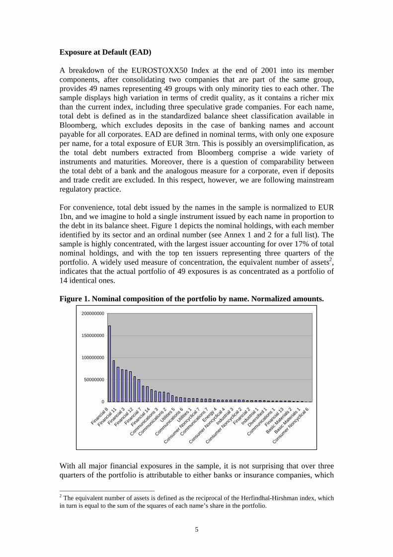
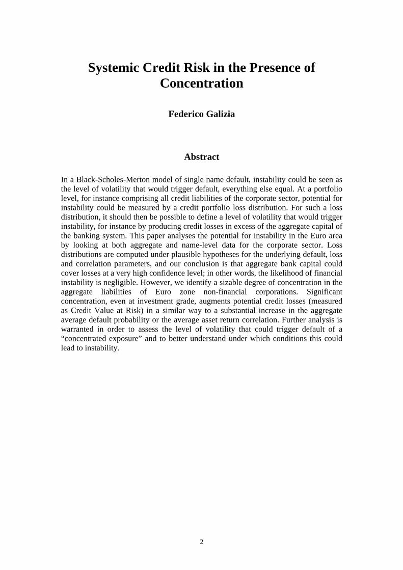
Exposure at Default (EAD) A breakdown of the EUROSTOXX50 Index at the end of 2001 into its member components, after consolidating two companies that are part of the same group, provides 49 names representing 49 groups with only minority ties to each other. The sample displays high variation in terms of credit quality, as it contains a richer mix than the current index, including three speculative grade companies. For each name, total debt is defined as in the standardized balance sheet classification available in Bloomberg, which excludes deposits in the case of banking names and account payable for all corporates. EAD are defined in nominal terms, with only one exposure per name, for a total exposure of EUR 3trn. This is possibly an oversimplification, as the total debt numbers extracted from Bloomberg comprise a wide variety of instruments and maturities. Moreover, there is a question of comparability between the total debt of a bank and the analogous measure for a corporate, even if deposits and trade credit are excluded. In this respect, however, we are following mainstream regulatory practice. For convenience, total debt issued by the names in the sample is normalized to EUR 1bn, and we imagine to hold a single instrument issued by each name in proportion to the debt in its balance sheet. Figure 1 depicts the nominal holdings, with each member identified by its sector and an ordinal number (see Annex 1 and 2 for a full list). The sample is highly concentrated, with the largest issuer accounting for over 17% of total nominal holdings, and with the top ten issuers representing three quarters of the portfolio. A widely used measure of concentration, the equivalent number of assets2, indicates that the actual portfolio of 49 exposures is as concentrated as a portfolio of 14 identical ones. Figure 1. Nominal composition of the portfolio by name. Normalized amounts.

0

50000000

100000000

150000000

200000000

Financ

ial 8

Financ

ial 11

Financ

ial 3

Financ

ial 12

Financ

ial 7

Financ

ial 14

Commun

icatio

ns 3

Commun

icatio

ns 2

Utilities

5

Commun

icatio

ns 6

Utilities

1

Consu

mer Non

cyclic

al 7

Commun

icatio

ns 7

Energy

4

Consu

mer Non

cyclic

al 4

Indus

trial 3

Consu

mer Non

cyclic

al 2

Financ

ial 2

Indus

trial 1

Diversi

fied 1

Commun

icatio

ns 1

Financ

ial 13

Basic

Materia

ls 2

Basic

Materia

ls 1

Consu

mer Non

cyclic

al 6

With all major financial exposures in the sample, it is not surprising that over three quarters of the portfolio is attributable to either banks or insurance companies, which

2 The equivalent number of assets is defined as the reciprocal of the Herfindhal-Hirshman index, which in turn is equal to the sum of the squares of each name’s share in the portfolio.

5

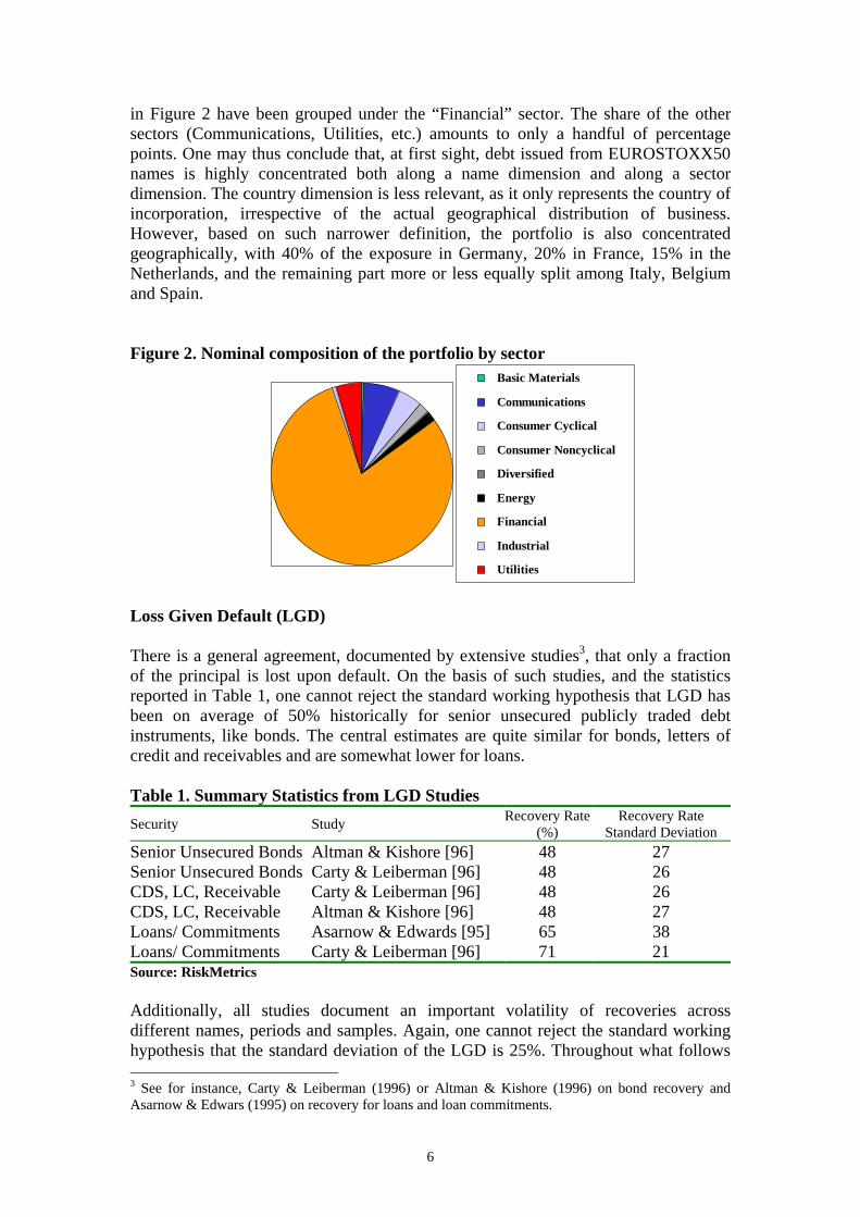
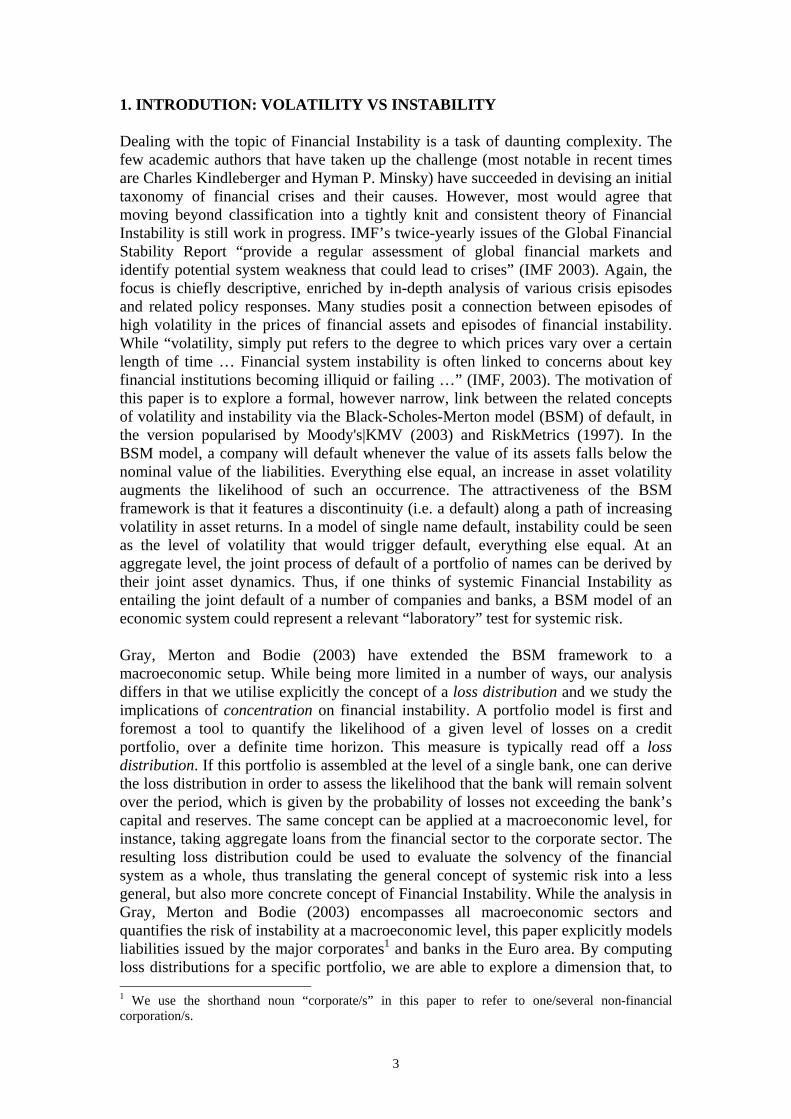
in Figure 2 have been grouped under the “Financial” sector. The share of the other sectors (Communications, Utilities, etc.) amounts to only a handful of percentage points. One may thus conclude that, at first sight, debt issued from EUROSTOXX50 names is highly concentrated both along a name dimension and along a sector dimension. The country dimension is less relevant, as it only represents the country of incorporation, irrespective of the actual geographical distribution of business. However, based on such narrower definition, the portfolio is also concentrated geographically, with 40% of the exposure in Germany, 20% in France, 15% in the Netherlands, and the remaining part more or less equally split among Italy, Belgium and Spain. Figure 2. Nominal composition of the portfolio by sector

Basic Materials

Communications

Consumer Cyclical

Consumer Noncyclical

Diversified

Energy

Financial

Industrial

Utilities

Loss Given Default (LGD) There is a general agreement, documented by extensive studies3, that only a fraction of the principal is lost upon default. On the basis of such studies, and the statistics reported in Table 1, one cannot reject the standard working hypothesis that LGD has been on average of 50% historically for senior unsecured publicly traded debt instruments, like bonds. The central estimates are quite similar for bonds, letters of credit and receivables and are somewhat lower for loans. Table 1. Summary Statistics from LGD Studies Security Study Recovery Rate

(%) Recovery Rate

Standard Deviation Senior Unsecured Bonds Altman & Kishore [96] 48 27 Senior Unsecured Bonds Carty & Leiberman [96] 48 26 CDS, LC, Receivable Carty & Leiberman [96] 48 26 CDS, LC, Receivable Altman & Kishore [96] 48 27 Loans/ Commitments Asarnow & Edwards [95] 65 38 Loans/ Commitments Carty & Leiberman [96] 71 21 Source: RiskMetrics Additionally, all studies document an important volatility of recoveries across different names, periods and samples. Again, one cannot reject the standard working hypothesis that the standard deviation of the LGD is 25%. Throughout what follows 3 See for instance, Carty & Leiberman (1996) or Altman & Kishore (1996) on bond recovery and Asarnow & Edwars (1995) on recovery for loans and loan commitments.

6

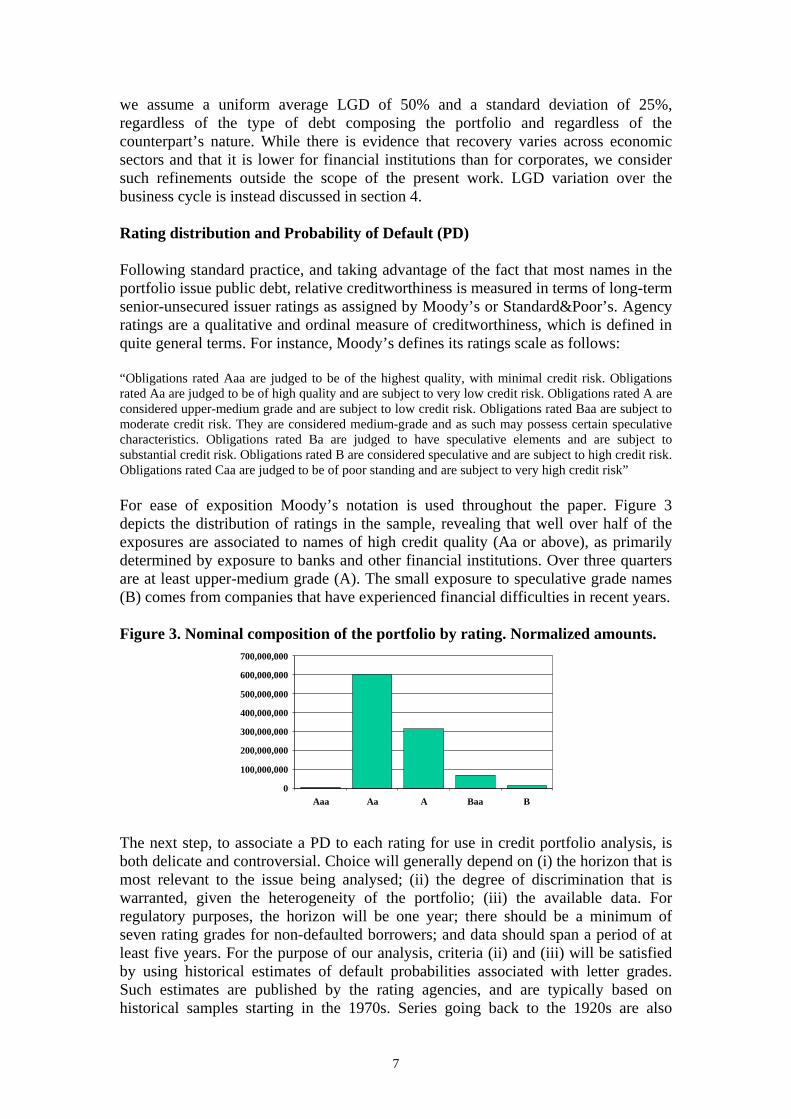
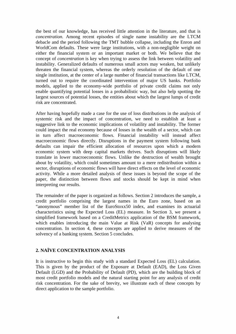
we assume a uniform average LGD of 50% and a standard deviation of 25%, regardless of the type of debt composing the portfolio and regardless of the counterpart’s nature. While there is evidence that recovery varies across economic sectors and that it is lower for financial institutions than for corporates, we consider such refinements outside the scope of the present work. LGD variation over the business cycle is instead discussed in section 4. Rating distribution and Probability of Default (PD) Following standard practice, and taking advantage of the fact that most names in the portfolio issue public debt, relative creditworthiness is measured in terms of long-term senior-unsecured issuer ratings as assigned by Moody’s or Standard&Poor’s. Agency ratings are a qualitative and ordinal measure of creditworthiness, which is defined in quite general terms. For instance, Moody’s defines its ratings scale as follows: “Obligations rated Aaa are judged to be of the highest quality, with minimal credit risk. Obligations rated Aa are judged to be of high quality and are subject to very low credit risk. Obligations rated A are considered upper-medium grade and are subject to low credit risk. Obligations rated Baa are subject to moderate credit risk. They are considered medium-grade and as such may possess certain speculative characteristics. Obligations rated Ba are judged to have speculative elements and are subject to substantial credit risk. Obligations rated B are considered speculative and are subject to high credit risk. Obligations rated Caa are judged to be of poor standing and are subject to very high credit risk” For ease of exposition Moody’s notation is used throughout the paper. Figure 3 depicts the distribution of ratings in the sample, revealing that well over half of the exposures are associated to names of high credit quality (Aa or above), as primarily determined by exposure to banks and other financial institutions. Over three quarters are at least upper-medium grade (A). The small exposure to speculative grade names (B) comes from companies that have experienced financial difficulties in recent years. Figure 3. Nominal composition of the portfolio by rating. Normalized amounts.

0

100,000,000

200,000,000

300,000,000

400,000,000

500,000,000

600,000,000

700,000,000

Aaa Aa A Baa B The next step, to associate a PD to each rating for use in credit portfolio analysis, is both delicate and controversial. Choice will generally depend on (i) the horizon that is most relevant to the issue being analysed; (ii) the degree of discrimination that is warranted, given the heterogeneity of the portfolio; (iii) the available data. For regulatory purposes, the horizon will be one year; there should be a minimum of seven rating grades for non-defaulted borrowers; and data should span a period of at least five years. For the purpose of our analysis, criteria (ii) and (iii) will be satisfied by using historical estimates of default probabilities associated with letter grades. Such estimates are published by the rating agencies, and are typically based on historical samples starting in the 1970s. Series going back to the 1920s are also

7

available, but arguably, they span economic episodes that are not relevant to the immediate future4. Realizing that there might be important differences across obligations rated within the same letter grade, in 1983 Moody’s introduced the “rating qualifiers” 1, 2 and 3, which are added after the letter grade to obtain an alphanumeric rating. For instance, the highest rated obligations within the letter grade Aa are rated Aa1, the lowest, Aa3. Historical default rates are also estimated for alphanumeric grades; however, the loss of degrees of freedom in estimating 17 instead of 7 PDs increases the volatility of central estimates. Default frequencies for alphanumeric grades often violate the basic requirement to be increasing along the rating scale. Concerning the risk horizon, the purposes of this exercise are best served if instead of the regulatory standard one-year horizon, a longer one is considered. Table 2 illustrates the reason for this choice. At a one-year horizon, the cumulative default probabilities for Aaa, Aa and A rated names are both negligible and indistinguishable. As the risk horizon increases, the number of default observations increases, thus rendering the estimates more reliable. Only reaching a three-year horizon the probability of default of Aa rated names ceases to be negligible and a clear distinction between this class and the two neighbouring ratings emerges. The difference in PD across ratings classes becomes more and more marked as the horizon increases, but arguably, pushing the horizon beyond 3-5 years will diminish the relevance of the study, as the reference sample becomes less and less representative of the Euro zone economy.

Table 2. Average Cumulative Default Rates 1970-2002 (Issuer Weighted) Fraction of issuers defaulting by the horizon (%)

Horizon (years) 1 2 3 4 5 Aaa 0 0 0 0.04 0.12 Aa 0.02 0.03 0.07 0.16 0.26 A 0.02 0.09 0.22 0.36 0.51 Baa 0.22 0.61 1.08 1.69 2.25 Ba 1.28 3.51 6.09 8.76 11.36 B 6.51 14.16 21.03 27.04 32.31 Caa-C 23.83 37.12 47.43 55.05 60.09 Investment-Grade 0.08 0.24 0.45 0.72 0.98 Speculative-Grade 4.99 10.05 14.66 18.67 22.18 All Corporates 1.59 3.19 4.64 5.9 6.96

Source: Moody’s 2003. Exhibit 44. It is noteworthy that default frequencies at a three-year horizon are of the same order of magnitude as “worst-case-one-year” default rates. The highest one-year default rate was recorded in 2002 for Investment Grade Corporates at 0.49% and in 2001 for Speculative Grade ones at 10.60%. As the sample consists mostly of the former, taking a three-year cumulative horizon is also representative of how much things did go wrong historically in one year over the 1970-2002 period. Most researchers refer to average cumulative default rates as “unconditional” default probabilities, since they span several business cycles. A “worst-case-one-year” default rate is instead thought of having a nature of “conditional” default probability. For instance, the aforementioned default rate of 0.49% recorded for investment grade issuers can be 4 One could certainly argue that there is a non-zero probability of a repeat of the Great Depression or a World War over the next thirty years, but most would agree that the probability of any such event hitting the Euro area over the next two-three years is indeed negligible.

8

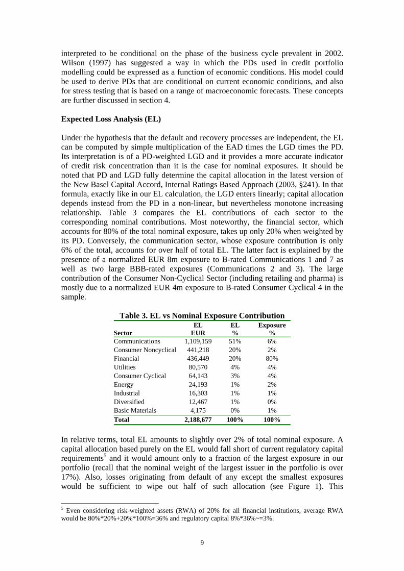
interpreted to be conditional on the phase of the business cycle prevalent in 2002. Wilson (1997) has suggested a way in which the PDs used in credit portfolio modelling could be expressed as a function of economic conditions. His model could be used to derive PDs that are conditional on current economic conditions, and also for stress testing that is based on a range of macroeconomic forecasts. These concepts are further discussed in section 4. Expected Loss Analysis (EL) Under the hypothesis that the default and recovery processes are independent, the EL can be computed by simple multiplication of the EAD times the LGD times the PD. Its interpretation is of a PD-weighted LGD and it provides a more accurate indicator of credit risk concentration than it is the case for nominal exposures. It should be noted that PD and LGD fully determine the capital allocation in the latest version of the New Basel Capital Accord, Internal Ratings Based Approach (2003, §241). In that formula, exactly like in our EL calculation, the LGD enters linearly; capital allocation depends instead from the PD in a non-linear, but nevertheless monotone increasing relationship. Table 3 compares the EL contributions of each sector to the corresponding nominal contributions. Most noteworthy, the financial sector, which accounts for 80% of the total nominal exposure, takes up only 20% when weighted by its PD. Conversely, the communication sector, whose exposure contribution is only 6% of the total, accounts for over half of total EL. The latter fact is explained by the presence of a normalized EUR 8m exposure to B-rated Communications 1 and 7 as well as two large BBB-rated exposures (Communications 2 and 3). The large contribution of the Consumer Non-Cyclical Sector (including retailing and pharma) is mostly due to a normalized EUR 4m exposure to B-rated Consumer Cyclical 4 in the sample.

Table 3. EL vs Nominal Exposure Contribution

Sector EL

EUR EL %

Exposure %

Communications 1,109,159 51% 6% Consumer Noncyclical 441,218 20% 2% Financial 436,449 20% 80% Utilities 80,570 4% 4% Consumer Cyclical 64,143 3% 4% Energy 24,193 1% 2% Industrial 16,303 1% 1% Diversified 12,467 1% 0% Basic Materials 4,175 0% 1% Total 2,188,677 100% 100%

In relative terms, total EL amounts to slightly over 2% of total nominal exposure. A capital allocation based purely on the EL would fall short of current regulatory capital requirements5 and it would amount only to a fraction of the largest exposure in our portfolio (recall that the nominal weight of the largest issuer in the portfolio is over 17%). Also, losses originating from default of any except the smallest exposures would be sufficient to wipe out half of such allocation (see Figure 1). This

5 Even considering risk-weighted assets (RWA) of 20% for all financial institutions, average RWA would be 80%*20%+20%*100%=36% and regulatory capital 8%*36%~=3%.

9

shortcoming is due to the fact that EL accounts for neither default correlation among exposures, nor the degree of concentration in the portfolio. To correct for the former, the proposal under the Basle II Internal Rating Based Approach, introduces an analytical formula that de facto augments the PD whenever correlation is non-zero6. Analytical approximations (e.g. the so “granularity adjustment” in Gordy (2002)) have also been proposed for portfolios that are not infinitely granular. In the next section, these issues are illustrated via numerical simulation. 3. THE EFFECT OF CORRELATION AND CONCENTRATION Loss distributions for credit portfolio risk are highly skewed and with fat tails, due to the relative infrequency of default events and to the fact that in unfavourable economics situations defaults tend to occur jointly. A model of correlation is needed to incorporate joint default risk in our sample portfolio. Once such a model is established, it is possible to compute a loss distribution by numerical methods and to discuss a set of portfolio-based concentration measures. A number of frameworks for this type of analysis have been proposed over the last few years and are surveyed in Saunders and Allen (2002). Koyluoglu and Hickman (1998) demonstrate that, subject to proper parameterisation, most frameworks could be harmonized to yield similar results. We rely on their argument to choose the model that is simplest to calibrate and implement, so that attention can be focussed on the results of the computations. A correlation model « à la CreditMetrics » Within the BSM framework, default occurs when negative asset returns bring the asset value below the nominal value of liabilities. The CreditMetrics methodology calibrates asset returns as a function of normally distributed equity returns. In practice, it is assumed that returns for each obligor are determined by an idiosyncratic factor as well as one or more stock market indexes. In this paper, each obligor is associated to only one such index; for instance, Financial 10 is mapped to the Morgan Stanley Capital International (MSCI) Banks Index for its country of incorporation, while Financial 14 is mapped to MSCI Banks Index for a different country. The asset correlation between these two banks will depend on the correlation between the two stock market indexes as well as the weights of each respective idiosyncratic factor. Following the methodology suggested in the CreditMetrics (1997 and 2003) documentation, we determine the latter weight as an inverse function of the size of the obligor, measured by its total assets. Annex 1 contains the full list of obligors, their total assets, and the weight of the stock index mappings (measured in terms of the R-squared in a univariate regression). On average, asset correlation across obligors in the sample is substantial, of the order of 40%, as one would expect, due to the fact that equity returns across blue chips in the Euro area are highly correlated. Once asset returns are thus calibrated, the value of the default barrier is inferred as the percentile

6 The formula is ⎟⎟⎠

⎞⎜⎜⎝

⎛

−

Φ+ΦΦ

−−

ρρ

1)999.0()( 11 PD

, where Φ represents the cumulative function

for the standard normal distribution and 1−Φ its inverse, and ρ the average asset correlation in the portfolio. It is easy to see that, in the presence of zero correlation the formula returns PD (and the Basel formula reduces to a multiple of the EL). The result is greater than PD, for positive correlation.

10

of the asset return distribution corresponding to the PD associated to each obligor’s rating. Thus, default correlation is ultimately driven by a modified correlation of equity index returns.

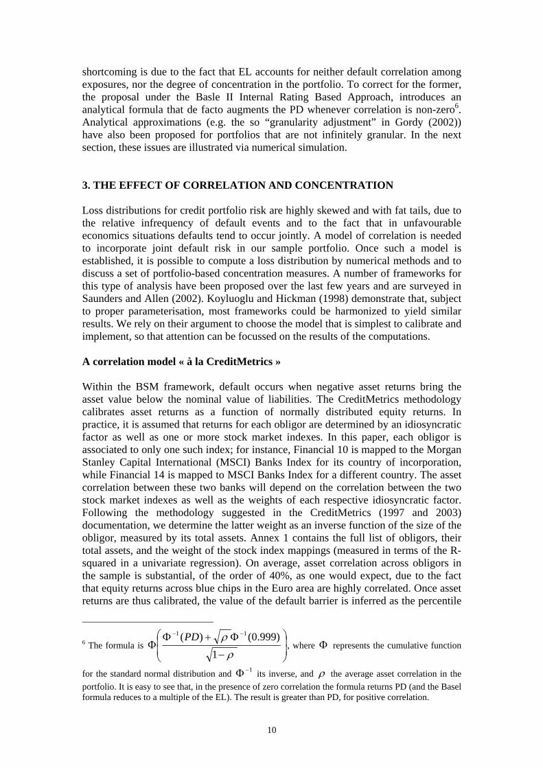
Figure 4. Horizon Value Distribution

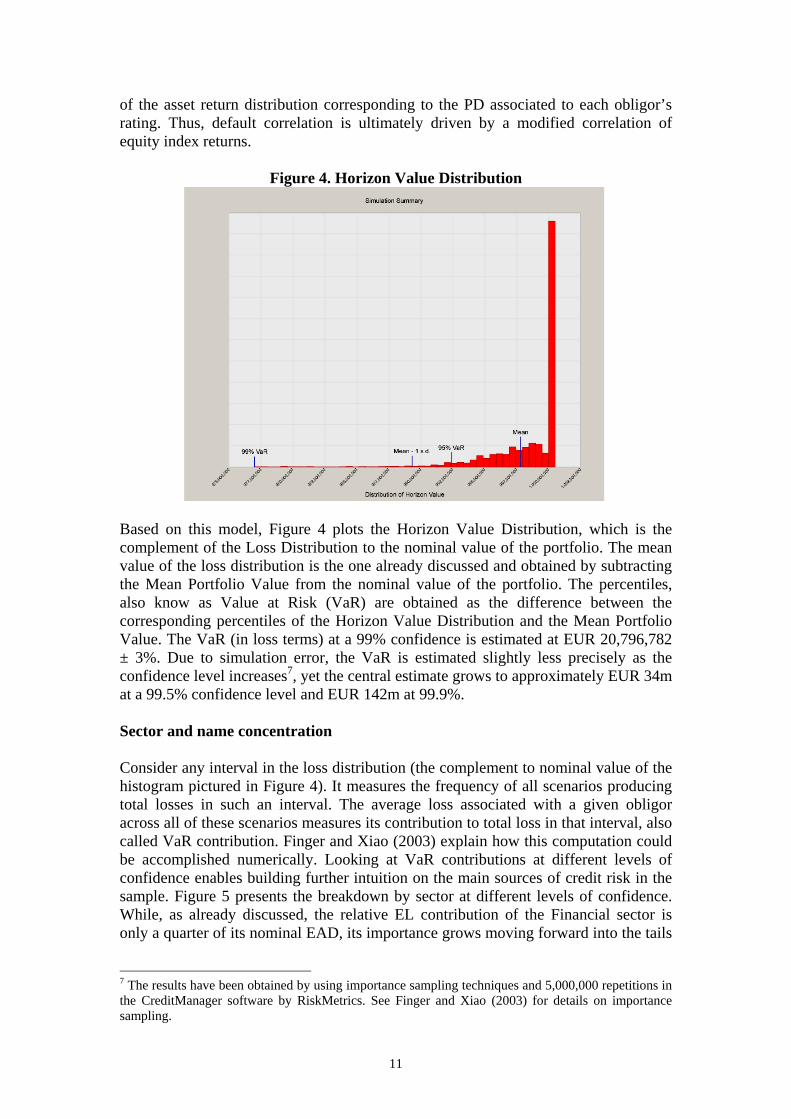
Based on this model, Figure 4 plots the Horizon Value Distribution, which is the complement of the Loss Distribution to the nominal value of the portfolio. The mean value of the loss distribution is the one already discussed and obtained by subtracting the Mean Portfolio Value from the nominal value of the portfolio. The percentiles, also know as Value at Risk (VaR) are obtained as the difference between the corresponding percentiles of the Horizon Value Distribution and the Mean Portfolio Value. The VaR (in loss terms) at a 99% confidence is estimated at EUR 20,796,782 ± 3%. Due to simulation error, the VaR is estimated slightly less precisely as the confidence level increases7, yet the central estimate grows to approximately EUR 34m at a 99.5% confidence level and EUR 142m at 99.9%. Sector and name concentration Consider any interval in the loss distribution (the complement to nominal value of the histogram pictured in Figure 4). It measures the frequency of all scenarios producing total losses in such an interval. The average loss associated with a given obligor across all of these scenarios measures its contribution to total loss in that interval, also called VaR contribution. Finger and Xiao (2003) explain how this computation could be accomplished numerically. Looking at VaR contributions at different levels of confidence enables building further intuition on the main sources of credit risk in the sample. Figure 5 presents the breakdown by sector at different levels of confidence. While, as already discussed, the relative EL contribution of the Financial sector is only a quarter of its nominal EAD, its importance grows moving forward into the tails

7 The results have been obtained by using importance sampling techniques and 5,000,000 repetitions in the CreditManager software by RiskMetrics. See Finger and Xiao (2003) for details on importance sampling.

11

of the loss distribution. At a 99.9% confidence level, the Financial sector represents approximately 90% of the total Value at Risk. Figure 5. Exposure, EL and VaR Contribution by sector

0%10%20%30%40%50%60%70%80%90%

100%

BookValue(1bn)

EL (2m) VaR 99%(21m)

VaR99.5%(34m)

VaR99.9%(142m)

Utilities

Industrial

Financial

Energy

Diversified

Consumer Noncyclical

Consumer Cyclical

Communications

Basic Materials

The explanation is straightforward, but nevertheless quite central to the understanding of systemic risk. As loss scenarios are ordered by increasing loss and decreasing likelihood along the distribution, one will encounter defaults of relatively riskier borrowers at low confidence levels. At higher confidence levels, less risky exposures begin to default. At very high confidence levels joint default begin to occur. Systemic risk is encountered at these higher percentiles in the loss distribution. This reasoning, however, only holds if no single obligor dominates the portfolio. Table 4. Top VaR contributors at different confidence levels Top ten contributions VaR 99.5% Top ten contributions VaR 99.9% Communications 2 3,333,232 Financial 8 67,372,534 Communications 3 3,259,372 Financial 9 10,902,895 Communications 7 3,224,454 Financial 10 8,462,587 Financial 11 2,691,770 Financial 1 6,903,279 Financial 14 2,271,389 Financial 12 5,322,734 Consumer Cyclical 1 1,824,415 Financial 11 5,235,778 Financial 3 1,560,210 Financial 15 5,096,058 Consumer Noncyclical 4 1,422,554 Financial 3 4,680,736 Utilities 2 1,050,698 Financial 14 3,862,672 Financial 1 972,450 Communications 7 2,336,584 Total 33,984,931 Total 141,982,236 An analysis of VaR contribution by name (see Table 4 and also Annex 2) clarifies the point further. The top contributors to the VaR99% and VaR99.5% are Baa-rated Communications 2 and 3 and B-rated Communications 7 with a total normalized exposure of less than EUR 50m. The top contributor to the VaR99.9% is instead a bank, A-rated, but with the largest normalized exposure in the portfolio of EUR

12

170m8. Whenever a default scenario involving such a large exposure is drawn, losses are “pushed to the tails” of the distribution. To understand why, let us recall that the VaR99.5% amounts to EUR 34m, while on average, LGD on this exposure will be EUR 85m. Thus, most of the increase from VaR99.5% to VaR 99.9% (i.e. from EUR 34m to EUR 142m) is explained by the additional EUR 85m of potential losses on the largest exposure in the sample. The intuition is further reinforced by observing that the second largest contributor at a 99.9% confidence, also a bank, is Aa-rated but with LGD that is only half the former. It seems that the highest tail contributions tend to come either from very large exposures, independently of their creditworthiness, or from highly rated exposures, everything else equal. There is thus something fundamentally different about large concentrations, that is not easily captured by any single capital allocation measure, but that instead requires in-depth analysis of the tails of the distribution at different confidence levels. The assumption of a granular portfolio, underlying the capital requirements proposed in the Consultative Paper on the New Basel Capital Accord (2003), may thus warrant reconsideration9. Other than exposure size and high ratings, an additional reason for the disproportionate weight of the financial sector at the highest confidence level is that average return correlation is significantly higher between financial institutions (60%) than it is within other sectors. This is a mechanical consequence of the CreditMetrics correlation model, where the larger the obligor the higher its weight in any given stock market index and consequently, the higher the systematic component of its returns. Higher return correlation increases the relative likelihood of infrequent events like joint defaults. Again, this implies that regulatory capital may need to consider contributions at different confidence levels. 4. MEASURING THE SOLVENCY OF A BANKING SYSTEM. DOES CONCENTRATION MATTER? Overall, the 49 names in our sample have outstanding debt (excluding deposits) in excess of EUR 3trn. The sample contains nine Aa-rated banks (Financials 3, 6-7; 9-12, 14 and 15) and two A-rated ones (Financials 8 and 14). Collectively, these banks have total capital in excess of EUR 300bn, that is, in excess of 10% of nominal exposure. Such an order of magnitude is comparable to the estimates of risk computed in the previous section, where we found that the VaR at a 99.5% (99.9%) confidence level (over a three-year horizon) is approximately 3% (14%) of the normalized portfolio. Does this finding allow one to infer that the largest banks in the Euro area are solvent at a confidence level that is higher than 99.5% but lower then 99.9%, that is, there is more than one (but less then five) chance(s) in one thousand that cumulative losses on the portfolio over a three year period (or over one worst case year) will exceed their aggregate capital at EUR 300bn? While the above reasoning can only be taken as suggestive, one could argue that it is both too conservative and not conservative enough. One the one hand, the portfolio of these banks is much more diversified, as it extends well beyond the EUROSTOXX50 8 Since a considerable fraction of the liabilities of the bank in question is constituted by Aaa rated covered bonds, our results considerably overstate the concentration effect at this level of confidence. Once more, we should emphasise that any reference to a specific name is for illustrative purposes only. 9 The point is made explicitly in the IMF Staff Comments on the April 2003 Consultative Paper (2003).

13

names and, additionally, there are banks and capital market investors outside the EUROSTOXX50 which share the risk on these large corporates, either in a direct form or in the form of a credit derivative. This is particularly true since the portfolio is largely composed by bank bonds, a substantial part of which is held by the household sector. On the other hand, the portfolio of a specific institution might be more concentrated than the average on a risky corporate, contributing disproportionately to systemic risk. Aggregate flow-of-funds date provide some additional elements. In its Monthly Bulletin, the European Central Bank publishes statistics on loans to the government, non-financial corporations and households. At the end of the second quarter of 2003, total loans outstanding exceeded EUR 8trn, with EUR 1trn taken by the government sector, and the remaining EUR 7trn split halfway between the corporate and household sector. Of the total loans, over EUR 7trn had been extended by Euro Area Monetary Financial Institutions (MFI). Interestingly, outstanding bonds, issued by the corporate sector, amount to little over EUR 0.5trn. The total capital and reserves of the aforementioned MFI exceed EUR 1trn. Thus, if one omits loans granted outside the Euro area, capital and reserves cover approximately 14% of the outstanding face value of MFI loans. An interesting question to ask is at which level of confidence such capital and reserves would be sufficient to ensure solvency of the banking system taken as an aggregate. We believe there is a meaningful way in which such a question could be addressed. For the sake of illustration, analysis is restricted to the corporate sector, leaving retail and inter-bank exposures as a topic for further research. The first subsection below presents the main argument, while the second sub-section discusses the robustness of the results under stress tested parameter values. Should concentration make a difference to the capital requirements? Participating banks to the several Basle II Quantitative Impact Studies have been asked to estimate capital requirements using the IRB formulas, that is, under the assumption that their portfolios were infinitely granular. One should be able to perform a similar exercise, based on aggregate data from the ECB Bulletin, by properly segment the total exposure, for instance by country and by rating class, and to obtain a reasonable estimate of the aggregate loss distribution. However, overlooking the presence of potential concentration in the credit aggregates might lead to a systematic underestimation of aggregate risk. Together, the thirty-eight corporates in our sample have outstanding debt close to EUR 1trn, so that they represent approximately one quarter of total corporate debt outstanding, including both loans and bonds. The largest debt, excluding banks, is Aa-rated Financial 3’s at EUR 230bn (approximately 5% of a total corporate debt of EUR 4trn), followed by A-rated Consumer Cyclical 1 with EUR 80m and Baa-rated Communications 3 with EUR 70m. Some further exploration thus appears to be justified. In order to assess the potential impact from concentration, we fix the attention on total corporate sector debt, which, for illustrative purposes, we quantify at EUR 4trn and compute loss distributions under several hypotheses for average PD, LGD, and asset correlation. Loss distributions are initially computed under the assumption that the portfolio is infinitely granular, using an approximation analogous to the IRB formula,

14

which is built in the CreditManager software10. Subsequently, we explicitly model the exposure represented by the thirty-eight corporate names in the EuroStoxx50 and compare the resulting loss distributions at various levels of confidence to assess the impact of concentration. The parameters for the infinitely granular portfolio are calibrated as follows:

• PD. The recently released Moody’s study “Default and Recovery Rates of European Corporate Bond Issuers, 1985–2002” estimates an average default rate of 2.9% for all corporates in 2002, the worst year in the sample. While cumulative default rates are not yet available for European corporates, the study observes that one-year transition matrices for European and US bond issuers are quite similar. Thus, consistently with our hypothesis derived from casual observation of US data, that “worst-case-one-year” default rates are of the same order of magnitude as three-year cumulative default rates, we estimate average credit quality of European bond issuers to be lower then Baa (3y default rate of 1.08%) but higher than Ba (3y default rate of 6.09%). For illustrative purposes, two sets of simulations are run using the IRB formula, the first one based on a PD of 3% and the last on 6%. The latter, higher level is possibly more reflective of companies that do not issue public debt, but only have access to bank credit.

• Asset correlation. Based on Moody’s¦KMV data for listed European companies and calibrating loss distributions for a single factor, Lopez (2002) estimates correlation as low as 10.0% and as high as 22.5% depending on the size of the companies as well as their PD. This range is well below the average correlation applied to our EuroStoxx 50 portfolio, but consistent with the fact that the sector includes obligors of different sizes and from diverse countries. Lopez (2002) also finds that lower asset correlations tend to be associated to higher PDs. Applying the most recent IRB formula for correlation to our chosen range of PD between 3% and 6% one finds asset correlation as high as 15% and as low as 9%, respectively. For illustrative purposes, we tabulate two round levels of correlation (10% and 20%).

• LGD. The working hypothesis of 50% average LGD, with a standard deviation of 25% is maintained.

The first figure in each cell in the first row of Table 5 reports the VaR11 estimates for an infinitely granular portfolio of EUR 4trn. The second figure in each cell of the same table, obtained by assuming that a loan pool of approximately EUR 3bn plus our sample of 38 non-bank obligors make up the total portfolio of EUR 4trn, should gauge the impact of concentration. The < or the > sign separates the two figures, the

10 Xiao and Finger (2003) demonstrate that, with proper parameterisation, the IRB-type formulas enable approximating the loss distribution for a portfolio with a large enough number of homogeneous obligors. 11 The CreditManager software requires input of the number of exposures comprising a loan pool, but Xiao & Finger (2003) find that a couple thousand exposures are sufficient to ensure convergence of the loss distribution, under most parameter values. Estimates of the equivalent number of corporate exposures for the Euro area would probably yield an order of magnitude of at least several hundred thousands, which is well beyond the number needed for convergence. As a consequence we arbitrarily set the number of exposures at 2,000. Sensitivity tests run using 5,000 and 10,000 exposures confirm the intuition.

15

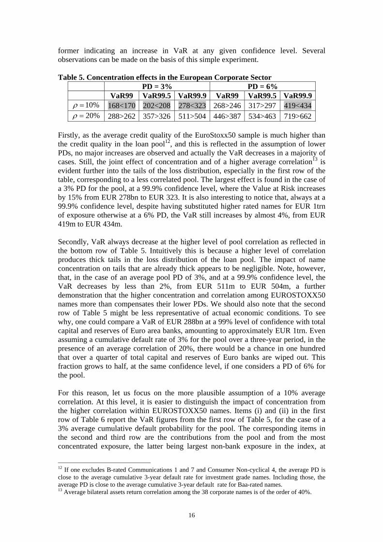
former indicating an increase in VaR at any given confidence level. Several observations can be made on the basis of this simple experiment. Table 5. Concentration effects in the European Corporate Sector

PD = 3% PD = 6% VaR99 VaR99.5 VaR99.9 VaR99 VaR99.5 VaR99.9

%10=ρ 168<170 202<208 278<323 268>246 317>297 419<434 %20=ρ 288>262 357>326 511>504 446>387 534>463 719>662

Firstly, as the average credit quality of the EuroStoxx50 sample is much higher than the credit quality in the loan pool12, and this is reflected in the assumption of lower PDs, no major increases are observed and actually the VaR decreases in a majority of cases. Still, the joint effect of concentration and of a higher average correlation13 is evident further into the tails of the loss distribution, especially in the first row of the table, corresponding to a less correlated pool. The largest effect is found in the case of a 3% PD for the pool, at a 99.9% confidence level, where the Value at Risk increases by 15% from EUR 278bn to EUR 323. It is also interesting to notice that, always at a 99.9% confidence level, despite having substituted higher rated names for EUR 1trn of exposure otherwise at a 6% PD, the VaR still increases by almost 4%, from EUR 419m to EUR 434m. Secondly, VaR always decrease at the higher level of pool correlation as reflected in the bottom row of Table 5. Intuitively this is because a higher level of correlation produces thick tails in the loss distribution of the loan pool. The impact of name concentration on tails that are already thick appears to be negligible. Note, however, that, in the case of an average pool PD of 3%, and at a 99.9% confidence level, the VaR decreases by less than 2%, from EUR 511m to EUR 504m, a further demonstration that the higher concentration and correlation among EUROSTOXX50 names more than compensates their lower PDs. We should also note that the second row of Table 5 might be less representative of actual economic conditions. To see why, one could compare a VaR of EUR 288bn at a 99% level of confidence with total capital and reserves of Euro area banks, amounting to approximately EUR 1trn. Even assuming a cumulative default rate of 3% for the pool over a three-year period, in the presence of an average correlation of 20%, there would be a chance in one hundred that over a quarter of total capital and reserves of Euro banks are wiped out. This fraction grows to half, at the same confidence level, if one considers a PD of 6% for the pool. For this reason, let us focus on the more plausible assumption of a 10% average correlation. At this level, it is easier to distinguish the impact of concentration from the higher correlation within EUROSTOXX50 names. Items (i) and (ii) in the first row of Table 6 report the VaR figures from the first row of Table 5, for the case of a 3% average cumulative default probability for the pool. The corresponding items in the second and third row are the contributions from the pool and from the most concentrated exposure, the latter being largest non-bank exposure in the index, at

12 If one excludes B-rated Communications 1 and 7 and Consumer Non-cyclical 4, the average PD is close to the average cumulative 3-year default rate for investment grade names. Including those, the average PD is close to the average cumulative 3-year default rate for Baa-rated names. 13 Average bilateral assets return correlation among the 38 corporate names is of the order of 40%.

16

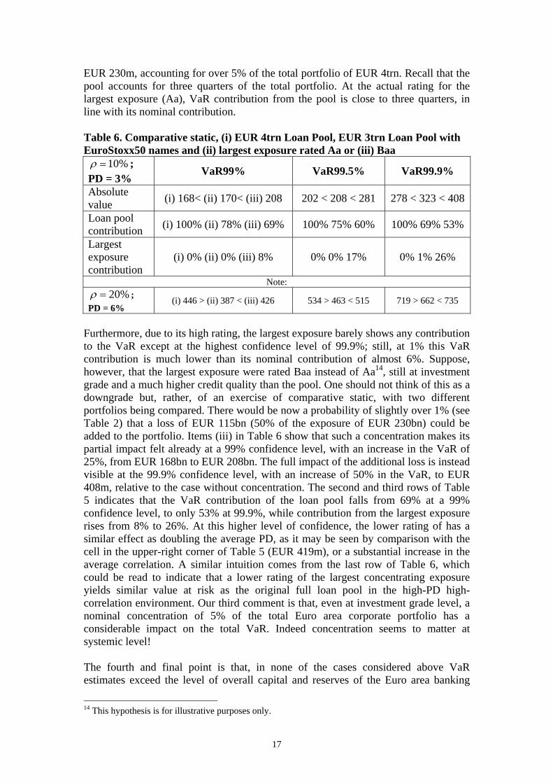
EUR 230m, accounting for over 5% of the total portfolio of EUR 4trn. Recall that the pool accounts for three quarters of the total portfolio. At the actual rating for the largest exposure (Aa), VaR contribution from the pool is close to three quarters, in line with its nominal contribution. Table 6. Comparative static, (i) EUR 4trn Loan Pool, EUR 3trn Loan Pool with EuroStoxx50 names and (ii) largest exposure rated Aa or (iii) Baa

%10=ρ ; PD = 3%

VaR99% VaR99.5% VaR99.9%

Absolute value (i) 168< (ii) 170< (iii) 208 202 < 208 < 281 278 < 323 < 408

Loan pool contribution (i) 100% (ii) 78% (iii) 69% 100% 75% 60% 100% 69% 53%

Largest exposure contribution

(i) 0% (ii) 0% (iii) 8% 0% 0% 17% 0% 1% 26%

Note: %20=ρ ;

PD = 6% (i) 446 > (ii) 387 < (iii) 426 534 > 463 < 515 719 > 662 < 735

Furthermore, due to its high rating, the largest exposure barely shows any contribution to the VaR except at the highest confidence level of 99.9%; still, at 1% this VaR contribution is much lower than its nominal contribution of almost 6%. Suppose, however, that the largest exposure were rated Baa instead of Aa14, still at investment grade and a much higher credit quality than the pool. One should not think of this as a downgrade but, rather, of an exercise of comparative static, with two different portfolios being compared. There would be now a probability of slightly over 1% (see Table 2) that a loss of EUR 115bn (50% of the exposure of EUR 230bn) could be added to the portfolio. Items (iii) in Table 6 show that such a concentration makes its partial impact felt already at a 99% confidence level, with an increase in the VaR of 25%, from EUR 168bn to EUR 208bn. The full impact of the additional loss is instead visible at the 99.9% confidence level, with an increase of 50% in the VaR, to EUR 408m, relative to the case without concentration. The second and third rows of Table 5 indicates that the VaR contribution of the loan pool falls from 69% at a 99% confidence level, to only 53% at 99.9%, while contribution from the largest exposure rises from 8% to 26%. At this higher level of confidence, the lower rating of has a similar effect as doubling the average PD, as it may be seen by comparison with the cell in the upper-right corner of Table 5 (EUR 419m), or a substantial increase in the average correlation. A similar intuition comes from the last row of Table 6, which could be read to indicate that a lower rating of the largest concentrating exposure yields similar value at risk as the original full loan pool in the high-PD high-correlation environment. Our third comment is that, even at investment grade level, a nominal concentration of 5% of the total Euro area corporate portfolio has a considerable impact on the total VaR. Indeed concentration seems to matter at systemic level! The fourth and final point is that, in none of the cases considered above VaR estimates exceed the level of overall capital and reserves of the Euro area banking

14 This hypothesis is for illustrative purposes only.

17

system (approximately EUR 1trn) and that estimates are closest only at levels of confidence that are 99.9% or higher. The next subsection tests the robustness of this result, by considering stress scenarios for the main parameter values. Cyclical effects and parameter calibration While the illustrative purpose of our exercise is served by the simplest of assumptions, and the main conclusions are unlikely to be overturned by a more sophisticated parameterization, recent research on (i) the probabilities of default, (ii) the asset return correlations and (iii) the recovery rate is worth discussing. In particular, we should consider implications of the extensive literature, surveyed in Allen and Saunders (2003) and Altman, Resti and Sironi (2003), which has studied interrelated parameter variation over the business cycle. The aforementioned conclusion, that bank reserves for the Euro area are sufficient to cover losses at all but quasi-certain confidence levels, is found to be robust under a wider range of parameters as suggested in the literature. Unconditional vs conditional probabilities of default We have tabulated results for PD levels (a low level of 3% and a high level of 6%) that are based on historical default frequencies for European non-financial rated corporates. The assumptions are consistent with three-year cumulative default frequencies as well as worst-year frequencies. According to Moody’s global statistics, three-year average cumulative default frequencies for all rated bonds amounted to 4.65% in the 1920-2003 period, 4.71% in 1970-2003 and 6.06% during the latest cycle (1994-2003). The corresponding figure for annual default frequencies (post 1970) attained the maximum value in 2001 globally and for the US, respectively at 3.8% and 4.7%, and in 2002 for European names, at 2.9%. In “dollar-weighted” terms, the global maximum was 5.29%, again in 2001. This long historical record supports our chosen range of PDs. Average cumulative default frequencies are typically interpreted as “unconditional” default probabilities as opposed to year-by-year default frequencies, which are “conditional” on the macroeconomic environment in a given year. With particular reference to default time series for speculative grade ratings, both Wilson (1997) and Moody’s (1999) are able to fit regressions with very high R-squares, explaining default rates for speculative names in terms of a parsimonious set of variables (macroeconomic in Wilson (1997), both macroeconomic and rating variables in Moody’s (1999)). An even more parsimonious characterization is provided by Moody’s¦KMV EDF methodology, where default frequencies are expressed a non-parametric fit to “distance-to-default” measures, in turn derived from a Black-Scholes-Merton setup (see Moody’s¦KMV (2003)). These methods yield “forward-looking” default probabilities and at a first look, one might be tempted to dismiss our results on grounds that we are using unconditional and backward looking default probabilities instead of conditional, forward looking ones. Such a dismissal would be only superficially correct, for at least three sets of reasons. Firstly, our assumed range includes worst-year PDs, which are by their nature conditional on the economic environment of the year in which they are produced. Secondly, long-term cumulative averages are conditional on long-term averages for the explanatory variables. Thirdly, even if we were to employ a formal model of conditional default probabilities, as long

18

as such a model is estimated on the historical period and on the available data, predicted default frequencies will be in the range that has been historically observed. A more serious concern to be addressed is whether the economic environment that is implicitly assumed by our calculations (i.e. worst year since 1970s or average year since the 1920s) provides a satisfactory characterization of future credit risks. If one looks for worst-year default frequencies all the way back to the 1920s, a maximum value of 8.4% is recorded for all corporates, presumably in the late twenties or early thirties15. This should be interpreted as being conditional on a severe recession coupled with a prolonged stock market crash, an extreme monetary tightening and bank runs. Such conditions have neither being repeated since, nor are representative of the average economic environment underlying the average cumulative defaults. For the sake of illustration, one could re-run simulations for a fully granular portfolio in the presence of a 9% PD and assuming a 20% asset correlation. The VaR at a 99.9% attains EUR 849 bn, still short of total capital and reserve of the Euro area banking system. Asset vs default correlation The assumed levels for asset correlation, a low level of 10% and a high level of 20% are not out of line with available estimates over a long time horizon. Moody’s¦KMV (2002) estimates median asset return correlation of approximately 20% for Utility firms in their global database of listed companies, 18% for the largest Industrial firms and 10% for all Industrial firms. Considering that the European Corporate sector is mostly composed of unlisted companies, which are likely to be smaller and less correlated, the assumed range appears to be conservative enough. Similar considerations apply to the correlation model “à la CreditMetrics” applied to EuroStoxx50 companies. This yields a median asset correlation in excess of 40% for the 38 corporate names, which is, if anything too conservative16. What, however, matters for computing a loss distribution is not asset, but rather default correlation, and the latter depends on both the former and the assumed PD level. Under jointly normally distributed assets returns, the default correlation between any two identical obligors is approximately 3%, for PD=3% and asset correlation of 10% and it grows to approximately 6%, for PD=6% and asset correlation of 20%. Based on the S&P default database and on the period 1981-2001, De Servigny and Renault (2003) estimate an average default correlation of 0.1% and 1.7% annually and respectively for US investment grade and speculative grade names. Using the same data on the period 1981-1999, Nagpal and Bahar (2001) had previously found a default correlation of 0.02% and respectively 1.08% for investment grade and speculative grade names at a one-year horizon, growing to 0.29% and 5.50% over a seven-year horizon. Zhou (2001), consistently with Lucas (1995), estimates a 6% default correlation between Ba rated companies at a two-year horizon17. Since average cumulative default frequencies for all corporates are

15 Moody’s (2004), Exhibit 25 - Annual Global Issuer-Weighted Default Rate Descriptive Statistics, 1920-2003. 16 These levels result from applying the model in Finger and Xiao (2003). The logical concern that overestimating correlation could lead to a similar overestimation of concentration was addressed by the comparative static in Table 6. 17 Unfortunately, Zhou’s (2001) does not provide estimates over a three-year horizon for Ba names.

19

typically found to be lower but close to the corresponding frequencies for Ba-rated names, one could consider these findings to provide an upper bound. In conclusion, the default correlation ranging between 3% and 6% that is implicit in our analysis appears significantly more conservative than justified available historical experience. Anecdotic evidence is still often cited that both equity correlation and default correlation increase during downturns. To gain a quantitative insight on the implications of this claim, we have run an infinitely granular EUR 4trn portfolio under a PD of 9% and an asset correlation of 30%, both extreme, but plausible in a depression scenario. Default correlation levels are much higher, at least of the order of 15%. We find that losses at a confidence level of 99.9% exceed EUR 1trn, while they are still well below at a 99.5% level. In other words, only a truly depressed scenario, characterized by both high PDs and abnormally high asset correlation could endanger solvency of the Euro area banking system on aggregate; and, even then, only with a probability of one-in-a-thousand times. Countercyclical Loss Given Default If one measures LGD from distressed bond values following a default event, it is only natural to find a strong positive correlation driven by the business and credit cycle. Moody’s (2004) documents a long-term average recovery rate of 40% on corporate bonds in the period 1982-2003, with peak levels close to 50% in 1987 and again in 1997, and troughs below 30% in 1990 and again in 2000 and 2001. Altman, Sironi and Resti (2002) study in detail the determinant of this relationship and its implications on regulatory capital. To examine the potential impact of this dynamics on our results, we apply the same test performed by Altman, Sironi and Resti (2002), who use “a second-degree polynomial to model the link between LGDs and empirical default rates, so that LGD is 50% when default rates are at their 20-year average (2%), LGD is 60% when default rates hit their 20-year maximum (5%) and LGD is 40% when default rates hit their 20-year low (0%)”. If an average LGD of 60% is used to replicate Table 5 and 6 above (while keeping constant the standard deviation of LGD), all percentiles of the loss distribution increase by 10%, with none of the key findings being affected. 5. CONCLUSIONS AND FURTHER RESEARCH Significant concentration, even at investment grade, augments potential credit losses (measured as Credit Value at Risk) in a similar way to a substantial increase in the aggregate average default probability or the average asset return correlation in a credit portfolio. We are however sceptical about presence of any systemic threat in the Euro area. Firstly, aggregate capital and reserves of the Euro zone banking system should cover potential losses at a very high confidence level under normal economic conditions. Secondly, having heuristically demonstrated that concentration does have an impact on the capital requirements of the banking sector, one should also recognise that such an impact was measured only in terms of “potential” rather than “actual” losses. Thirdly, even when highly concentrated defaults occur in practice, like it has been the case over the past business cycle, the ability of the banking system to spread losses across different institutions, including sellers of credit protection outside the

20

banking sector, is such that the solidity of the system should still be preserved. Thus, if only a fraction of the Euro zone banks’ capital is at risk, and such a risk only comes with a small probability, the likelihood of systemic insolvency has to be limited. A number of caveats qualify the aforementioned. Firstly, the analysis is greatly simplified and it relies on standardized parameter calibration. A recent assessment of the state of the art in estimating PDs and especially correlations (Koyluoglu, Wilson and Yague 2003) makes a strong case for being humble about achievements to date. Secondly, historical, backward looking default probabilities and correlations are at the base of our model. In a full application of the BSM framework, both default probabilities and correlations are determined by the corporate asset values and by their volatility in a forward-looking way. Thirdly, one needs embedding the problem within a macroeconomic framework. There is a tight relationship between default rates and macroeconomic variables (Wilson 1997), suggesting that one should be able to embed default dynamics in a macroeconomic model, via explicit modelling of corporate asset values. The idea has been expressed in a different and more general context by Tobin (1980, 1992), whose lifelong work was centred on understanding the interaction between asset stocks, assets flows and macroeconomic activity in the presence of uncertainty. The interest of the latter exercise would be to model the borderline between a situation that is not threatening (e.g. a circumscribed corporate or banking default episode) and a system-wide financial crisis. Within the BSM framework for credit risk analysis, such borderline is measured in terms of volatility. High levels of volatility translate into higher probability that asset values will fall below the default barrier for a higher number of obligors; these higher potential losses in turn increase uncertainty and further depress asset prices. Along a path of increasing volatility, losses at higher levels of confidence will be realized. However, the impact will be radically different in a concentrated portfolio from a granular one. In a granular portfolio, losses will build up gradually. In a concentrated portfolio, one might observe large losses in correspondence of defaults from concentrated exposures, along a path of increasing volatility. Thus, instability will be more likely in an economy characterized by concentrated credit risk than in one where credit risk is more granular, everything else equal. In the absence of significant concentration, and in the presence of well functioning automatic stabilisers, corporate insolvencies associated with an economic downturn may weaken the banking sector and affect the wealth of bondholders and shareholders. Presumably this will lead to increased precautionary savings and lower consumption. Negative pressure on consumption will also derive from the likely temporary upsurge in unemployment; but this negative effect on aggregate demand will likely be softened by higher public expenditure for unemployment benefits. What if instead a large concentrated default were to occur on top of economic conditions characterized by higher default rates and higher correlation? Such an episode would be more likely to trigger insolvency in the banking sector, which, other than further destroying accumulated financial wealth, would also likely disrupt resource allocation and impact economic flows. Progress in analysing these questions is well under way. Regulators, Statistical Agencies and Rating Agencies are devoting important resources to the task of collecting and analysing credit risk data. While these studies have to date been chiefly employed in business applications, an increasing number of economists in various

21

institutions is focusing on credit risk and financial instability. Notably, Gray, Merton and Bodie (2003) have initiated the extension of contingent claim analysis from the corporate sector to a wider macroeconomic framework. Dynamic stochastic general equilibrium models developed for monetary policy analysis now often include financial asset dynamics. Some of these models might suffer from aggregation fallacies and their empirical application is still quite limited, but clearly have the potential to take up the challenge.

22

REFERENCES Allen Linda and Anthony Saunders, “A Survey of Cyclical Effects in Credit Risk Measurement Models”, BIS Working Papers No 126, January 2003 Altman Edward I, Andrea Resti and Andrea Sironi, “The link between default and recovery rates: effects on the procyclicality of regulatory capital ratios”, BIS Working Papers No 113, July 2002 Altman, Edward I., and Vellore M. Kishore, "Almost Everything You Wanted to Know about Recoveries on Defaulted Bonds", Financial Analysts Journal, November/December 1996 Asarnow, Elliot, and David Edwards. “Measuring Loss on Defaulted Bank Loans: A 24-Year Study,” The Journal of Commercial Lending, March 1995 Bank for International Settlements (Basel II), “The New Basel Capital Accord: Third Consultative Paper” (Basel II), April 2003 Bank for International Settlements, “Quantitative Impact Study 3 - Overview of Global Results”, May 2003 Barakova, I., Carey, M., 2003. How quickly do troubled banks recapitalize? With implications for portfolio VaR credit loss horizons. Working Paper, Federal Reserve Board Carty, Lea V., and Dana Lieberman, “Corporate Bond Defaults and Default Rates 1938-1995,” Moody’s Investors Service, Global Credit Research, January 1996 ______, “Defaulted Bank Loan Recoveries,” Moody’s Investors Service, Global Credit Research, Special Report, November 1996 De Servigny Arnaud and Olivier Renault, “Correlation Evidence”, Risk, July 2003 European Central Bank, Monthly Bulletin, December 2003 Finger Christopher C. and Jerry Yi Xiao, CreditManager Product Technical Notes, 2003 Gordy M. “A Risk Factor Model Foundation for Ratings-Based Capital Rules”, the Board of Governors of the Federal Reserve System, 2002 Gray Dale F., Robert C. Merton and Zvi Bodie, “A New Framework for Analyzing and Managing Macrofinancial Risk of an Economy”, MF Risk Working Paper 1, 2003 International Monetary Fund (IMF), Global Financial Stability Report, September 2003 Kindleberger , Charles. P., Manias, Panics, and Crashes: A History of Financial Crises, New York: John Wiley & Sons; 4th edition, 2001 Koyluoglu, H.Ugur, Tom Wilson and Miguel Yague, “The Eternal Challenge of Understanding Imperfections”, Mercer Oliver Wyman, 2003 Koyluoglu, H.Ugur and Andrew Hickman, “Reconcilable Differences”, Risk, October 1998 Lopez Jose A., “The Empirical Relationship between Average Asset Correlation, Firm Probability of Default and Asset Size”, Working Paper, Federal Reserve Bank of San Francisco, 2002

23

Merton, Robert C. "On the Pricing of Corporate Debt: The Risk Structure of Interest Rates", Journal of Finance, Vol. 29, 1974 Minsky, Hyman. P., John Maynard Keynes, New York, Columbia University Press, 1975 _____, “The Financial Instability Hypothesis: Capitalistic Processes and The Behavior of the Economy” in C.P. Kindleberger and J.-P. Lafargue, Financial Crises: Theory, History and Policy, Cambridge, Cambridge University Press, 1982 Moody’s Investor’s Service, “Predicting Default Rates: A Forecasting Model For Moody's Issuer-Based Default Rates”, 1999 Moody’s Investor Service, “Default & Recovery Rates of Corporate Bond Issuers” January 2004 Moody's|KMV’s Crosbie, Peter J., and Jeffrey R. Bohn, “Modeling Default Risk”, December 2003 Moody's|KMV’s Zen, Bin, and Jing Zhang, “Measuring Credit Correlations: Equity Correlations Are Not Enough!”, January 2002 Nagpal Krishan and Reza Bahar, “Measuring Default Correlation”, Risk, March 2001 RiskMetrics’ Gupton, Greg M., Christopher C. Finger, and Mickey Bhatia, "CreditMetrics™ -- Technical Document", J.P. Morgan, April 1997 Saunders Anthony and Linda Allen, Credit Risk Measurement: New Approaches to Value at Risk and Other Paradigms, 2nd Edition, New York, John Wiley & Sons, March 15, 2002 Tobin James, “Money”, The New Palgrave Dictionary of Money and Finance, 1992 ______, Asset Accumulation and Economic Activity, Chicago, The University of Chicago Press, 1980 Wilson Tom, “Portfolio Credit Risk, Part I & Part II”, Risk 10 (9&10), 1997

24

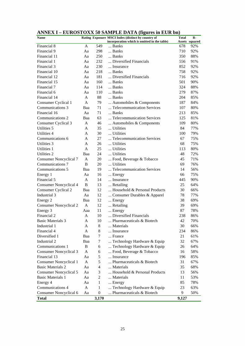
ANNEX I – EUROSTOXX 50 SAMPLE DATA (figures in EUR bn) Name Rating Exposure MSCI Index (distinct by country of

incorporation which is omitted in the table) Total Assets

R- squared

Financial 8 A 549 ... Banks 678 92% Financial 9 Aa 298 ... Banks 710 92% Financial 11 Aa 250 ... Banks 350 88% Financial 1 Aa 232 ... Diversified Financials 556 91% Financial 3 Aa 230 ... Insurance 852 92% Financial 10 Aa 218 ... Banks 758 92% Financial 12 Aa 181 ... Diversified Financials 716 92% Financial 15 Aa 160 ... Banks 501 90% Financial 7 Aa 114 ... Banks 324 88% Financial 6 Aa 110 ... Banks 279 87% Financial 14 A 88 ... Banks 204 85% Consumer Cyclical 1 A 79 ... Automobiles & Components 187 84% Communications 3 Baa 71 ... Telecommunication Services 107 80% Financial 16 Aa 71 ... Banks 213 85% Communications 2 Baa 63 ... Telecommunication Services 125 81% Consumer Cyclical 3 A 46 ... Automobiles & Components 109 80% Utilities 5 A 35 ... Utilities 84 77% Utilities 4 A 30 ... Utilities 100 79% Communications 6 A 27 ... Telecommunication Services 67 75% Utilities 3 A 26 ... Utilities 68 75% Utilities 1 A 25 ... Utilities 113 80% Utilities 2 Baa 24 ... Utilities 48 72% Consumer Noncyclical 7 A 20 ... Food, Beverage & Tobacco 45 71% Communications 7 B 20 ... Utilities 69 76% Communications 5 Baa 19 ... Telecommunication Services 14 56% Energy 1 Aa 16 ... Energy 66 75% Financial 5 A 14 ... Insurance 445 90% Consumer Noncyclical 4 B 13 ... Retailing 25 64% Consumer Cyclical 2 Baa 12 ... Household & Personal Products 30 66% Industrial 3 Aa 12 ... Consumer Durables & Apparel 78 77% Energy 2 Baa 12 ... Energy 38 69% Consumer Noncyclical 2 A 12 ... Retailing 39 69% Energy 3 Aaa 11 ... Energy 87 78% Financial 2 A 10 ... Diversified Financials 238 86% Basic Materials 3 A 10 ... Pharmaceuticals & Biotech 42 70% Industrial 1 A 8 ... Materials 30 66% Financial 4 A 8 ... Insurance 234 86% Diversified 1 Baa 7 ... France 21 61% Industrial 2 Baa 7 ... Technology Hardware & Equip 32 67% Communications 1 B 6 ... Technology Hardware & Equip 26 64% Consumer Noncyclical 3 A 6 ... Food, Beverage & Tobacco 16 58% Financial 13 Aa 5 ... Insurance 196 85% Consumer Noncyclical 1 A 5 ... Pharmaceuticals & Biotech 31 67% Basic Materials 2 Aa 4 ... Materials 35 68% Consumer Noncyclical 5 Aa 3 ... Household & Personal Products 13 56% Basic Materials 1 Aa 2 ... Materials 11 53% Energy 4 Aa 1 ... Energy 85 78% Communications 4 A 1 ... Technology Hardware & Equip 23 63% Consumer Noncyclical 6 Aa 0 ... Pharmaceuticals & Biotech 9 50% Total 3,170 9,127

25

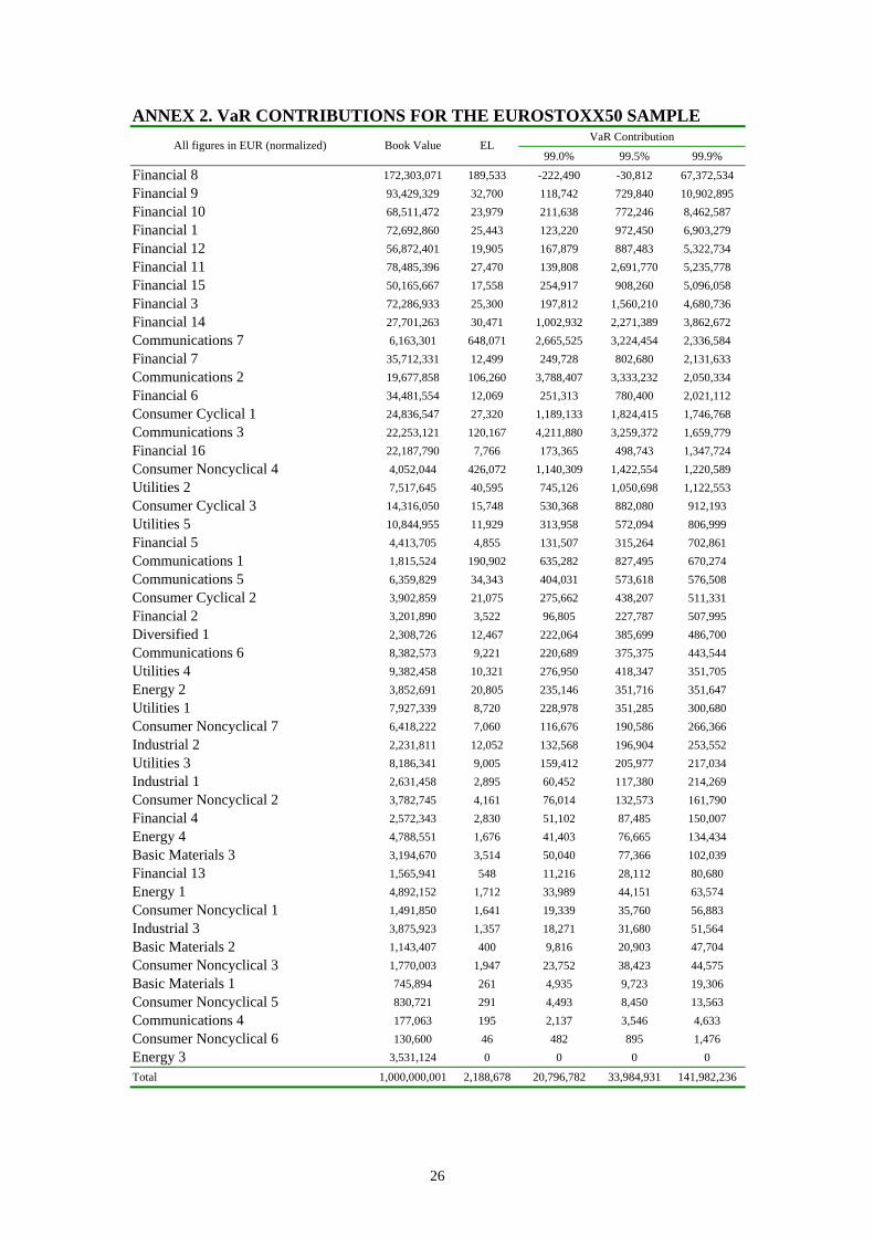
ANNEX 2. VaR CONTRIBUTIONS FOR THE EUROSTOXX50 SAMPLE VaR Contribution

All figures in EUR (normalized) Book Value EL 99.0% 99.5% 99.9%

Financial 8 172,303,071 189,533 -222,490 -30,812 67,372,534 Financial 9 93,429,329 32,700 118,742 729,840 10,902,895 Financial 10 68,511,472 23,979 211,638 772,246 8,462,587 Financial 1 72,692,860 25,443 123,220 972,450 6,903,279 Financial 12 56,872,401 19,905 167,879 887,483 5,322,734 Financial 11 78,485,396 27,470 139,808 2,691,770 5,235,778 Financial 15 50,165,667 17,558 254,917 908,260 5,096,058 Financial 3 72,286,933 25,300 197,812 1,560,210 4,680,736 Financial 14 27,701,263 30,471 1,002,932 2,271,389 3,862,672 Communications 7 6,163,301 648,071 2,665,525 3,224,454 2,336,584 Financial 7 35,712,331 12,499 249,728 802,680 2,131,633 Communications 2 19,677,858 106,260 3,788,407 3,333,232 2,050,334 Financial 6 34,481,554 12,069 251,313 780,400 2,021,112 Consumer Cyclical 1 24,836,547 27,320 1,189,133 1,824,415 1,746,768 Communications 3 22,253,121 120,167 4,211,880 3,259,372 1,659,779 Financial 16 22,187,790 7,766 173,365 498,743 1,347,724 Consumer Noncyclical 4 4,052,044 426,072 1,140,309 1,422,554 1,220,589 Utilities 2 7,517,645 40,595 745,126 1,050,698 1,122,553 Consumer Cyclical 3 14,316,050 15,748 530,368 882,080 912,193 Utilities 5 10,844,955 11,929 313,958 572,094 806,999 Financial 5 4,413,705 4,855 131,507 315,264 702,861 Communications 1 1,815,524 190,902 635,282 827,495 670,274 Communications 5 6,359,829 34,343 404,031 573,618 576,508 Consumer Cyclical 2 3,902,859 21,075 275,662 438,207 511,331 Financial 2 3,201,890 3,522 96,805 227,787 507,995 Diversified 1 2,308,726 12,467 222,064 385,699 486,700 Communications 6 8,382,573 9,221 220,689 375,375 443,544 Utilities 4 9,382,458 10,321 276,950 418,347 351,705 Energy 2 3,852,691 20,805 235,146 351,716 351,647 Utilities 1 7,927,339 8,720 228,978 351,285 300,680 Consumer Noncyclical 7 6,418,222 7,060 116,676 190,586 266,366 Industrial 2 2,231,811 12,052 132,568 196,904 253,552 Utilities 3 8,186,341 9,005 159,412 205,977 217,034 Industrial 1 2,631,458 2,895 60,452 117,380 214,269 Consumer Noncyclical 2 3,782,745 4,161 76,014 132,573 161,790 Financial 4 2,572,343 2,830 51,102 87,485 150,007 Energy 4 4,788,551 1,676 41,403 76,665 134,434 Basic Materials 3 3,194,670 3,514 50,040 77,366 102,039 Financial 13 1,565,941 548 11,216 28,112 80,680 Energy 1 4,892,152 1,712 33,989 44,151 63,574 Consumer Noncyclical 1 1,491,850 1,641 19,339 35,760 56,883 Industrial 3 3,875,923 1,357 18,271 31,680 51,564 Basic Materials 2 1,143,407 400 9,816 20,903 47,704 Consumer Noncyclical 3 1,770,003 1,947 23,752 38,423 44,575 Basic Materials 1 745,894 261 4,935 9,723 19,306 Consumer Noncyclical 5 830,721 291 4,493 8,450 13,563 Communications 4 177,063 195 2,137 3,546 4,633 Consumer Noncyclical 6 130,600 46 482 895 1,476 Energy 3 3,531,124 0 0 0 0

Total 1,000,000,001 2,188,678 20,796,782 33,984,931 141,982,236

26