Embed Size (px)
Citation preview


System identification: introduction
1 / 54

Building mathematical models
The design of a controller/observer requires a mathematical modeldescribing the behaviour of the plant.
A model describes how the signals of the system are related to each other.
A model and a system are two different objects.
Different kinds of models:− mental or intuitive models. For example:
when driving a car, pushing the break decreases the speed.− graphical models. For example:
Bode diagram or step response of an LTI system;current-voltage characteristic of a diode.
− mathematical models, described by equations.
We will focus on mathematical models of dynamical systems, described, ingeneral, by differential or difference equations.
Mathematical models can be derived from:− first principle laws of physics, chemistry, biology, etc.
(physical modeling approach)− observed data generated by the system
(system identification approach)
2 / 54

System identification procedure
The system identification procedure involves three basic entities:
1 Data, which can be either recorded from specifically designed experimentsor from normal operations of the system.
2 Set of candidate models, obtained by specifying within which set of modelswe are going to look for a suitable one. Different kinds of models may bespecified (e.g., linear vs nonlinear; continuous time vs discrete time;deterministic vs stochastic, etc.). Two types of model sets:
− gray boxes. A model with some unknown parameters is derived fromphysical laws. The parameters are then estimated from data.
− black boxes. A model structure is chosen (e.g., linear models). Theparameters of the model do not reflect any physical consideration.
3 Rule to assess candidate models using data. This is the identificationmethod, used to determinate the “best” model in the set, guided by data.
3 / 54

Model validation
Test whether the estimated model is an “appropriate” representation ofthe system. Assess how the model relates to:
prior knowledge. Does the model adequately describes prior knownphysical behaviour of the system?
experimental data (not used for training). Compare the simulatedoutputs of the model with the observed outputs.
4 / 54

System identification loop
design of experiment Prior knowledge
perform experiment
collect data
choose model structure
estimate the model
validate the model
model
accepted
New data
Use it
YES
NO
5 / 54

References and educational material
L. Ljung, System identification: theory for the user. Prentice-Hall EnglewoodCliffs, NJ, 1999
T. Soderstrom and P. Stoica, System identification, Prentice Hall International,1989. Available online at: http://user.it.uu.se/~ps/ps.html
Parametric System Identification - theory and tools, R. De Callafon, University ofCalifornia San Diego,http://mechatronics.ucsd.edu/mae283a_10/index.html
IEEE CSS Technical Commettee on System Identification and Adaptive Control,http://system-identification.ieeecss.org
6 / 54

LTI systems
7 / 54

Input/Output representation
Given a discrete-time signal u(k), k = 0, 1, . . ., we define the (unilater) z-transform of u as
Z{u(k)} = U(z) =∞∑k=0
u(k)z−k
Z{u(k − d)} = Z{q−du(k)} = z−dU(z), d ∈ Z
Z {g(k) ∗ u(k)} = Z{ ∞∑
ℓ=0
g(ℓ)u(k − ℓ)
}= Z {G(q)u(k)} = G(z)U(z)
G(q)u(k)
-y(k)- G(z)
U(z)-
Y (z)-
Analogy between the time-domain operator G(q) and the DT transfer function G(z)
Thanks to this analogy, we can treat G(q) as polynomials in q. Product and ratiobetween G1(q) and G2(q) have a meaning!
Example: y(k) = b1q−1
1+a1q−1 u(k) → (1 + a1q−1)y(k) = b1q−1u(k)
8 / 54

Linear regression representation
Linear regression representation of the system:
y(k) = φ⊤(k)θ
θ: parameter vector, φ(k): regressor vector, typically containing past values of inputsand outputs.
φ(k) = [−y(k − 1) . . . − y(k − na) u(k) . . . u(k − nb)]⊤
θ = [a1 . . . ana b0 . . . bnb ]⊤
Writing out the product gives:
y(k) = G(q)u(k), G(q) =b0 + b1q−1 + · · ·+ bnbq
−nb
1 + a1q−1 + · · ·+ anaq−na
Non-linear systems can be easily represented in a linear regression form.Just include nonlinear terms (e.g., y 2(k − 1); u(k)y(k − 1)) in the regressor!
9 / 54

Least-squares estimation
10 / 54

Linear least-squares
Consider a model in the linear regression form: M : y(k, θ) = φ⊤(k)θ
Define the residuals as ε(k, θ) = y(k)− y(k, θ) = y(k)− φ⊤(k)θ
ε(k, θ) represents the error between output observations and model outputs y(k, θ)
Least-squares (LS) estimate:
θLS = argminθ
N∑k=1
ε2(k, θ) = argminθ
N∑k=1
(y(k)− φ⊤(k)θ
)2
= argminθ
∥Y − Φθ∥2
Y =
y(1)
.
.
.y(N)
, Φ =
φ⊤(1)
.
.
.
φ⊤(N)
Solution of the QP problem:
θLS :∂ ∥Y − Φθ∥2
∂θ= 0
→ θLS =(Φ⊤Φ
)−1Φ⊤Y =
(N∑
k=1
φ(k)φ⊤(k)
)−1 N∑k=1
φ(k)y(k)
Matlab: θLS = Φ \ Y
11 / 54

Linear least-squares
Consider a model in the linear regression form: M : y(k, θ) = φ⊤(k)θ
Define the residuals as ε(k, θ) = y(k)− y(k, θ) = y(k)− φ⊤(k)θ
ε(k, θ) represents the error between output observations and model outputs y(k, θ)
Least-squares (LS) estimate:
θLS = argminθ
N∑k=1
ε2(k, θ) = argminθ
N∑k=1
(y(k)− φ⊤(k)θ
)2= argmin
θ∥Y − Φθ∥2
Y =
y(1)
.
.
.y(N)
, Φ =
φ⊤(1)
.
.
.
φ⊤(N)
Solution of the QP problem:
θLS :∂ ∥Y − Φθ∥2
∂θ= 0 → θLS =
(Φ⊤Φ
)−1Φ⊤Y =
(N∑
k=1
φ(k)φ⊤(k)
)−1 N∑k=1
φ(k)y(k)
Matlab: θLS = Φ \ Y11 / 54

Linear least-squares: Cholesky factorization
θLS =(Φ⊤Φ
)−1Φ⊤Y
θLS is the solution of the set of linear equations:
Φ⊤ΦθLS = Φ⊤Y
Use Cholesky decomposition of Φ⊤Φ to solve the above system of linear equations, i.e.,
Φ⊤Φ = LL⊤ L : Lower Triangular Matrix
Matlab: L = chol(Φ⊤Φ,′ lower′)
Least-squares (LS) estimate:
LL⊤θLS = Φ⊤Y
⇓
Lz = Φ⊤Y , L⊤θLS = z
Solve the linear system Lz = Φ⊤Y through forward substitution
Solve the linear system L⊤θLS = z through backward substitution
12 / 54

Linear least-squares: QR factorization
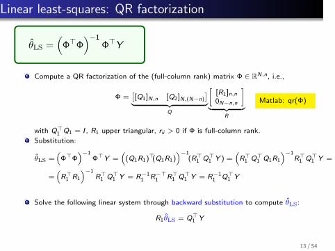
θLS =(Φ⊤Φ
)−1Φ⊤Y
Compute a QR factorization of the (full-column rank) matrix Φ ∈ RN,n, i.e.,
Φ =[[Q1]N,n [Q2]N,(N−n)
]︸ ︷︷ ︸Q
[[R1]n,n0N−n,n
]︸ ︷︷ ︸
R
with Q⊤1 Q1 = I , R1 upper triangular, rii > 0 if Φ is full-column rank.
Matlab: qr(Φ)
Substitution:
θLS =(Φ⊤Φ
)−1Φ⊤Y =
((Q1R1)
⊤(Q1R1))−1
(R⊤1 Q⊤
1 Y ) =(R⊤1 Q⊤
1 Q1R1
)−1R⊤1 Q⊤
1 Y =
=(R⊤1 R1
)−1R⊤1 Q⊤
1 Y = R−11 R−⊤
1 R⊤1 Q⊤
1 Y = R−11 Q⊤
1 Y
Solve the following linear system through backward substitution to compute θLS:
R1θLS = Q⊤1 Y
13 / 54

Linear least-squares: QR factorization
θLS =(Φ⊤Φ
)−1Φ⊤Y
Compute a QR factorization of the (full-column rank) matrix Φ ∈ RN,n, i.e.,
Φ =[[Q1]N,n [Q2]N,(N−n)
]︸ ︷︷ ︸Q
[[R1]n,n0N−n,n
]︸ ︷︷ ︸
R
with Q⊤1 Q1 = I , R1 upper triangular, rii > 0 if Φ is full-column rank.
Matlab: qr(Φ)
Substitution:
θLS =(Φ⊤Φ
)−1Φ⊤Y =
((Q1R1)
⊤(Q1R1))−1
(R⊤1 Q⊤
1 Y ) =(R⊤1 Q⊤
1 Q1R1
)−1R⊤1 Q⊤
1 Y =
=(R⊤1 R1
)−1R⊤1 Q⊤
1 Y = R−11 R−⊤
1 R⊤1 Q⊤
1 Y = R−11 Q⊤
1 Y
Solve the following linear system through backward substitution to compute θLS:
R1θLS = Q⊤1 Y
13 / 54

Recursive linear least squares
Estimate the parameters θLS recursively in time.
If there is an estimate θLS(k − 1) based on data up to time k − 1,then θLS(k) is computed based on a “simple” update of θLS(k − 1).
No need to record all data up to time k (low memory requirement).
Recursive LS can be easily modified to estimate time-varyingparameters.
14 / 54

Recursive linear least squares
θLS(k) =
(k∑
ℓ=1
φ(ℓ)φ⊤(ℓ)
)−1 k∑ℓ=1
φ(ℓ)y(ℓ)
P(k) =
(k∑
ℓ=1
φ(ℓ)φ⊤(ℓ)
)−1
, P−1(k) = P−1(k − 1) + φ(k)φ⊤(k)
θLS(k) = P(k)
(k−1∑ℓ=1
φ(ℓ)y(ℓ) + φ(k)y(k)
)
θLS(k) = P(k)(P−1(k − 1)θLS(k − 1) + φ(k)y(k)
)
θLS(k) = θLS(k − 1) + P(k)φ(k)︸ ︷︷ ︸K(k)
y(k)− φ⊤(k)θLS(k − 1)︸ ︷︷ ︸ε(k)
θLS(k) = θLS(k − 1) + K(k)ε(k)
K(k): gain
ε(k): error in the prediction of y(k) based on θLS(k − 1)
If the prediction error is “small”, the estimate θLS(k − 1) is “good” and
should not be modified “very much”
15 / 54

Recursive linear least squares
θLS(k) = θLS(k − 1) + P(k)φ(k)(y(k)− φ⊤(k)θLS(k − 1)
)P−1(k) = P−1(k − 1) + φ(k)φ⊤(k)
P−1(k) can be easily updated
Updating P(k) requires to invert P−1(k) at each time instant (time consuming)
Solution
P(k) =[P−1(k)
]−1
=[P−1(k − 1) + φ(k)φ⊤(k)
]−1
From Matrix Inversion Lemma:
P(k) = P(k − 1)− P(k − 1)φ(k)φ⊤(k)P(k − 1)
1 + φ⊤(k)P(k − 1)φ(k)
16 / 54

Recursive linear LS for real-time identification
Identify (slowly) time-varying parameters (due to slow time-variation of theprocess)
Useful for adaptive control
Introduce forgetting factor 0 < λ ≤ 1 in the cost function:
θ(k) = argminθ
k∑ℓ=1
λk−ℓ(y(ℓ)− φ⊤(ℓ)θ
)2
Decrease λ to forget information on past data faster
Recursive LS with forgetting factor
θ(k) = θ(k − 1) + P(k)φ(k)(y(k)− φ⊤(k)θLS(k − 1)
)P(k) =
1
λ
[P(k − 1)− P(k − 1)φ(k)φ⊤(k)P(k − 1)
λ+ φ⊤(k)P(k − 1)φ(k)
]
17 / 54

Estimate of FIR models through LS
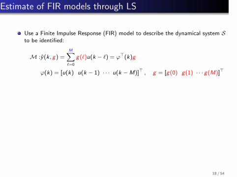
Use a Finite Impulse Response (FIR) model to describe the dynamical system Sto be identified:
M :y(k, g) =M∑ℓ=0
g(ℓ)u(k − ℓ)
= φ⊤(k)g
φ(k) = [u(k) u(k − 1) · · · u(k −M)]⊤ , g = [g(0) g(1) · · · g(M)]⊤
Good approximation if M is “large” and S is BIBO stable (which implieslim
ℓ→∞|g(ℓ)| = 0)
Collect N >> M observations of the pairs {u(k), y(k)}Nk=1
LS estimate of g :
g =(Φ⊤Φ
)−1
Φ⊤Y
18 / 54
Estimate of FIR models through LS
Use a Finite Impulse Response (FIR) model to describe the dynamical system Sto be identified:
M :y(k, g) =M∑ℓ=0
g(ℓ)u(k − ℓ) = φ⊤(k)g
φ(k) = [u(k) u(k − 1) · · · u(k −M)]⊤ , g = [g(0) g(1) · · · g(M)]⊤
Good approximation if M is “large” and S is BIBO stable (which implieslim
ℓ→∞|g(ℓ)| = 0)
Collect N >> M observations of the pairs {u(k), y(k)}Nk=1
LS estimate of g :
g =(Φ⊤Φ
)−1
Φ⊤Y
18 / 54

Estimate of FIR models through LS
g =(Φ⊤Φ
)−1
Φ⊤Y
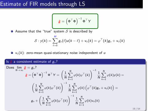
Assume that the “true” system S is described by
S : y(k) =M∑ℓ=0
go(ℓ)u(k − ℓ) + vo(k) = φ⊤(k)go + vo(k)
vo(k): zero-mean quasi-stationary noise independent of u
Is g a consistent estimate of go?
Does limN→∞
g = go?
g =(Φ⊤Φ
)−1Φ⊤Y =
(1
N
N∑k=1
φ(k)φ⊤(k)
)−11
N
N∑k=1
φ(k)y(k) =
(1
N
N∑k=1
φ(k)φ⊤(k)
)−11
N
N∑k=1
φ(k)(φ⊤(k)go + vo(k)
)=
go +
(1
N
N∑k=1
φ(k)φ⊤(k)
)−11
N
N∑k=1
φ(k)vo(k)
19 / 54

Estimate of FIR models through LS
g =(Φ⊤Φ
)−1
Φ⊤Y
Assume that the “true” system S is described by
S : y(k) =M∑ℓ=0
go(ℓ)u(k − ℓ) + vo(k) = φ⊤(k)go + vo(k)
vo(k): zero-mean quasi-stationary noise independent of u
Is g a consistent estimate of go?
Does limN→∞
g = go?
g =(Φ⊤Φ
)−1Φ⊤Y =
(1
N
N∑k=1
φ(k)φ⊤(k)
)−11
N
N∑k=1
φ(k)y(k) =
(1
N
N∑k=1
φ(k)φ⊤(k)
)−11
N
N∑k=1
φ(k)(φ⊤(k)go + vo(k)
)=
go +
(1
N
N∑k=1
φ(k)φ⊤(k)
)−11
N
N∑k=1
φ(k)vo(k)
19 / 54

Estimate of FIR models through LS
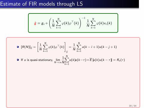
g = go+
(1
N
N∑k=1
φ(k)φ⊤(k)
)−1
1
N
N∑k=1
φ(k)vo(k)
[R(N)]ij =
[1
N
N∑k=1
φ(k)φ⊤(k)
]ij
=1
N
N∑k=1
u(k − i + 1)u(k − j + 1)
If u is quasi-stationary, limN→∞
1
N
N∑k=1
u(k)u(k−τ)=E [u(k)u(k − τ)] = Ru(τ)
Thus, limN→∞
R(N) = R∗ = E[φ(k)φ⊤(K)
]lim
N→∞
1
N
N∑k=1
φ(k)vo(k) = E [φ(k)vo(k)] = 0 , since u(k) is independent of
vo(k) and E [vo(k)] = 0.
limN→∞
g = go + R∗E [φ(k)vo(k)] = go
Thus, g is a consistent estimate of go
20 / 54

Estimate of FIR models through LS
g = go+
(1
N
N∑k=1
φ(k)φ⊤(k)
)−1
1
N
N∑k=1
φ(k)vo(k)
[R(N)]ij =
[1
N
N∑k=1
φ(k)φ⊤(k)
]ij
=1
N
N∑k=1
u(k − i + 1)u(k − j + 1)
If u is quasi-stationary, limN→∞
1
N
N∑k=1
u(k)u(k−τ)=E [u(k)u(k − τ)] = Ru(τ)
Thus, limN→∞
R(N) = R∗ = E[φ(k)φ⊤(K)
]lim
N→∞
1
N
N∑k=1
φ(k)vo(k) = E [φ(k)vo(k)] = 0 , since u(k) is independent of
vo(k) and E [vo(k)] = 0.
limN→∞
g = go + R∗E [φ(k)vo(k)] = go
Thus, g is a consistent estimate of go
20 / 54

Estimate of FIR models through LS
g = go+
(1
N
N∑k=1
φ(k)φ⊤(k)
)−1
1
N
N∑k=1
φ(k)vo(k)
[R(N)]ij =
[1
N
N∑k=1
φ(k)φ⊤(k)
]ij
=1
N
N∑k=1
u(k − i + 1)u(k − j + 1)
If u is quasi-stationary, limN→∞
1
N
N∑k=1
u(k)u(k−τ)=E [u(k)u(k − τ)] = Ru(τ)
Thus, limN→∞
R(N) = R∗ = E[φ(k)φ⊤(K)
]
limN→∞
1
N
N∑k=1
φ(k)vo(k) = E [φ(k)vo(k)] = 0 , since u(k) is independent of
vo(k) and E [vo(k)] = 0.
limN→∞
g = go + R∗E [φ(k)vo(k)] = go
Thus, g is a consistent estimate of go
20 / 54

Estimate of FIR models through LS
g = go+
(1
N
N∑k=1
φ(k)φ⊤(k)
)−1
1
N
N∑k=1
φ(k)vo(k)
[R(N)]ij =
[1
N
N∑k=1
φ(k)φ⊤(k)
]ij
=1
N
N∑k=1
u(k − i + 1)u(k − j + 1)
If u is quasi-stationary, limN→∞
1
N
N∑k=1
u(k)u(k−τ)=E [u(k)u(k − τ)] = Ru(τ)
Thus, limN→∞
R(N) = R∗ = E[φ(k)φ⊤(K)
]lim
N→∞
1
N
N∑k=1
φ(k)vo(k) = E [φ(k)vo(k)] = 0 , since u(k) is independent of
vo(k) and E [vo(k)] = 0.
limN→∞
g = go + R∗E [φ(k)vo(k)] = go
Thus, g is a consistent estimate of go
20 / 54

Estimate of FIR models through LS
g = go+
(1
N
N∑k=1
φ(k)φ⊤(k)
)−1
1
N
N∑k=1
φ(k)vo(k)
[R(N)]ij =
[1
N
N∑k=1
φ(k)φ⊤(k)
]ij
=1
N
N∑k=1
u(k − i + 1)u(k − j + 1)
If u is quasi-stationary, limN→∞
1
N
N∑k=1
u(k)u(k−τ)=E [u(k)u(k − τ)] = Ru(τ)
Thus, limN→∞
R(N) = R∗ = E[φ(k)φ⊤(K)
]lim
N→∞
1
N
N∑k=1
φ(k)vo(k) = E [φ(k)vo(k)] = 0 , since u(k) is independent of
vo(k) and E [vo(k)] = 0.
limN→∞
g = go + R∗E [φ(k)vo(k)] = go
Thus, g is a consistent estimate of go
20 / 54

Estimate of FIR models through LS: example
N = 300
Samples0 50 100
g
-1
-0.5
0
0.5
1
1.5
2
2.5Pulse response
trueestimate
Samples0 50 100 150 200
y-10
-5
0
5
10
output
trueestimate
SNR = 10 log10
(∑Nk=1 y
2(k)∑Nk=1 v
2o(k)
)= 6 db
BFR = 1−∑Nv
k=1 (y(k)− y(k))2∑Nvk=1 (y(k)− y)2
= 72%
21 / 54

Estimate of FIR models through LS: example
N = 500
Samples0 50 100
g
-1
-0.5
0
0.5
1
1.5
2
2.5Pulse response
trueestimate
Samples0 50 100 150 200
y-10
-5
0
5
10
output
trueestimate
SNR = 10 log10
(∑Nk=1 y
2(k)∑Nk=1 v
2o(k)
)= 6 db
BFR = 1−∑Nv
k=1 (y(k)− y(k))2∑Nvk=1 (y(k)− y)2
= 91%
22 / 54

Estimate of FIR models through LS: example
N = 1000
Samples0 50 100
g
-1
-0.5
0
0.5
1
1.5
2
2.5Pulse response
trueestimate
Samples0 50 100 150 200
y-10
-5
0
5
10
output
trueestimate
SNR = 10 log10
(∑Nk=1 y
2(k)∑Nk=1 v
2o(k)
)= 6 db
BFR = 1−∑Nv
k=1 (y(k)− y(k))2∑Nvk=1 (y(k)− y)2
= 96%
23 / 54

Estimate of FIR models through LS: example
N = 5000
Samples0 50 100
g
-1
-0.5
0
0.5
1
1.5
2
2.5Pulse response
trueestimate
Samples0 50 100 150 200
y-10
-5
0
5
10
output
trueestimate
SNR = 10 log10
(∑Nk=1 y
2(k)∑Nk=1 v
2o(k)
)= 6 db
BFR = 1−∑Nv
k=1 (y(k)− y(k))2∑Nvk=1 (y(k)− y)2
= 99%
24 / 54

Estimate of FIR models through LS: example
N = 10000
Samples0 50 100
g
-1
-0.5
0
0.5
1
1.5
2
2.5Pulse response
trueestimate
Samples0 50 100 150 200
y-10
-5
0
5
10
output
trueestimate
SNR = 10 log10
(∑Nk=1 y
2(k)∑Nk=1 v
2o(k)
)= 6 db
BFR = 1−∑Nv
k=1 (y(k)− y(k))2∑Nvk=1 (y(k)− y)2
= 99.7%
25 / 54

Estimate of ARX models through LS
y(k) = G(q)u(k) + H(q)e(k)
Gu-
y- ev?-
H
e?
+
AutoRegressive with eXogenous input (ARX) model structure:
G(q) =B(q)
A(q)=
b1q−1 + · · ·+ bnbq
−nb
1 + a1q−1 + · · ·+ anaq−na
H(q) =1
A(q)=
1
1 + a1q−1 + · · ·+ anaq−na
Corresponding input/output relationship
y(k) = −a1y(k − 1)− · · · − anay(k − na) + b1u(k − 1) + · · ·+ bnbu(k − nb) + e(k)
Unknown parameter vector: θ = [a1 . . . ana b1 . . . bnb ]⊤
Regressor vector: φ = [−y(k − 1) . . . − y(k − na) u(k − 1) . . . u(k − nb)]⊤
Output representation: y(k) = φ⊤(k)θ + e(k)
26 / 54

Estimate of ARX models through LS
Output representation: y(k) = φ⊤(k)θ + e(k)
Model structure: M : y(k, θ) = φ⊤(k)θ (linear regression)
LS estimate: θLS = argminθ
∥Y − Φθ∥2 =(Φ⊤Φ
)−1
Φ⊤Y
Assume the “true” system is described by S : y(k) = φ⊤(k)θo + e(k)
Is θLS a consistent estimate of θo?
Does limN→∞
θLS = θo?
θLS =(Φ⊤Φ
)−1Φ⊤Y =
(1
N
N∑k=1
φ(k)φ⊤(k)
)−11
N
N∑k=1
φ(k)y(k) =
(1
N
N∑k=1
φ(k)φ⊤(k)
)−11
N
N∑k=1
φ(k)(φ⊤(k)θo + e(k)
)=
θo +
(1
N
N∑k=1
φ(k)φ⊤(k)
)−11
N
N∑k=1
φ(k)e(k)
27 / 54

Estimate of ARX models through LS
θLS = θo+
(1
N
N∑k=1
φ(k)φ⊤(k)
)−1
1
N
N∑k=1
φ(k)e(k)
R(N) =1
N
N∑k=1
φ(k)φ⊤(k) is filled out with the estimate of auto/cross
covariance function estimates
If u is quasi-stationary, limN→∞
R(N) = R∗
limN→∞
1
N
N∑k=1
φ(k)e(k) = E [φ(k)e(k)] = E [φ(k)]E [e(k)] = 0, since φ(k) is
independent of e(k) and E [e(k)] = 0.
limN→∞
θLS = θo + R∗E [φ(k)e(k)] = θo
Thus, θLS is a consistent estimate of θo
28 / 54

Estimate of LPV-ARX models through LS
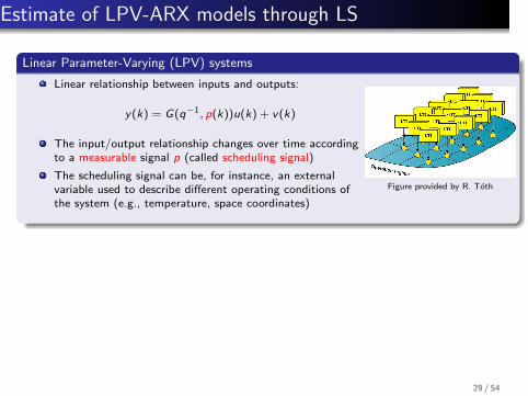
Linear Parameter-Varying (LPV) systems
Linear relationship between inputs and outputs:
y(k) = G(q−1, p(k))u(k) + v(k)
The input/output relationship changes over time accordingto a measurable signal p (called scheduling signal)
The scheduling signal can be, for instance, an externalvariable used to describe different operating conditions ofthe system (e.g., temperature, space coordinates)
Figure provided by R. Toth
LPV-ARX models
A(q−1, p(k))y(k) = B(q−1, p(k))u(k) + e(k), e white
A(q−1, p(k)) = 1 +
na∑i=1
ai (p(k))q−i , B(q−1, p(k)) =
nb∑j=1
bj (p(k))q−j
ai (p(k)) and bj (p(k)) are a-priori parametrized functions of p(k) (e.g., polynomials):
ai (p(k)) = ai,0 +
nl∑l=1
ai,lpl (k), bj (p(k)) = bj,0 +
nl∑l=1
bj,lpl (k)
29 / 54
Estimate of LPV-ARX models through LS
Linear Parameter-Varying (LPV) systems
Linear relationship between inputs and outputs:
y(k) = G(q−1, p(k))u(k) + v(k)
The input/output relationship changes over time accordingto a measurable signal p (called scheduling signal)
The scheduling signal can be, for instance, an externalvariable used to describe different operating conditions ofthe system (e.g., temperature, space coordinates)
Figure provided by R. Toth
LPV-ARX models
A(q−1, p(k))y(k) = B(q−1, p(k))u(k) + e(k), e white
A(q−1, p(k)) = 1 +
na∑i=1
ai (p(k))q−i , B(q−1, p(k)) =
nb∑j=1
bj (p(k))q−j
ai (p(k)) and bj (p(k)) are a-priori parametrized functions of p(k) (e.g., polynomials):
ai (p(k)) = ai,0 +
nl∑l=1
ai,lpl (k), bj (p(k)) = bj,0 +
nl∑l=1
bj,lpl (k)
29 / 54

Estimate of LPV-ARX models through LS
LPV-ARX models: example
A(q−1, p(k))y(k) = B(q−1, p(k))u(k) + e(k), e white
Example:
y(k) =− [a1,0 + a1,1p(k)] y(k − 1) + [b1,0 + b1,1p(k)] u(k − 1) + e(k)
y(k) =[−y(k − 1) −p(k)y(k − 1) u(k − 1) p(k)u(k − 1)]︸ ︷︷ ︸φ⊤(k)
a1,0a1,1b1,0b1,1
︸ ︷︷ ︸
θ
+ e(k)
Estimate θ through least-squares
Consistency is guaranteed if e is white
30 / 54

Inconsistency of LS: OE case
y(k) = G(q)u(k) + H(q)e(k)
Gu-
y- eη?-
H
e?
+
Output Error (OE) model structure:
G(q) =B(q)
A(q)=
b1q−1 + · · ·+ bnbq
−nb
1 + a1q−1 + · · ·+ anaq−na
H(q) =1
Corresponding input/output relationship
yo(k) =− a1yo(k − 1)− · · · − anayo(k − na) + b1u(k − 1) + · · ·+ bnbu(k − nb)
y(k) =yo(k) + e(k)
Unknown parameter vector: θ = [a1 . . . ana b1 . . . bnb ]⊤
Regressor vector: φ = [−y(k − 1) . . . − y(k − na) u(k − 1) . . . u(k − nb)]⊤
Output representation: y(k) = φ⊤(k)θ + e(k) + a1e(k − 1) + · · ·+ anae(k − na)︸ ︷︷ ︸v(k)
v(k) is not white!
31 / 54

Inconsistency of LS: OE case
Output representation: y(k) = φ⊤(k)θ + v(k)
Model structure: M : y(k, θ) = φ⊤(k)θ (linear regression)
LS estimate: θLS = argminθ
∥V ∥2 = argminθ
∥Y − Φθ∥2 =(Φ⊤Φ
)−1
Φ⊤Y
Assume the “true” system is described by S : y(k) = φ⊤(k)θo + v(k)
Is θLS a consistent estimate of θo?
Does limN→∞
θLS = θo?
θLS =(Φ⊤Φ
)−1Φ⊤Y =
(1
N
N∑k=1
φ(k)φ⊤(k)
)−11
N
N∑k=1
φ(k)y(k) =
(1
N
N∑k=1
φ(k)φ⊤(k)
)−11
N
N∑k=1
φ(k)(φ⊤(k)θo + v(k)
)=
θo +
(1
N
N∑k=1
φ(k)φ⊤(k)
)−11
N
N∑k=1
φ(k)v(k)
32 / 54

Inconsistency of LS: OE case
θLS = θo+
(1
N
N∑k=1
φ(k)φ⊤(k)
)−1
1
N
N∑k=1
φ(k)v(k)
R(N) =1
N
N∑k=1
φ(k)φ⊤(k) is filled out with the estimate of auto/cross
covariance function estimates
If u is quasi-stationary, limN→∞
R(N) = R∗
limN→∞
1
N
N∑k=1
φ(k)v(k) = E [φ(k)v(k)] = 0 since φ(k) is correlated with v(k)
Thus, θLS is not a consistent estimate of θo
33 / 54

Instrumental Variable Methods
34 / 54

Instrumental Variables (IV)
y(k) = G(q)u(k) + H(q)e(k)
Gu-
y- ev?-
H
e?
+
Given a model structure A(q−1)y(k) = B(q−1)u(k) + v(k), LS provides aconsistent estimate of the “true” system parameters only when {v(k)} is notcorrelated with the regressor (equivalently, if v is white).
Instrumental Variables (IV) methods provide solutions to guarantee consistencyalso when {v(k)} is correlated with the regressor
35 / 54

Instrumental Variables (IV): main idea
θLS =(Φ⊤Φ
)−1
Φ⊤Y =
(N∑
k=1
φ(k)φ⊤(k)
)−1 N∑k=1
φ(k)y(k)
Instrumental Variables Estimate
Chose a vector z(k), called instrument, with the same dimension of the regressorφ(k) and such that
E [z(k)v(k)] = 0 (i.e., z(k) is not correlated with v(k))
Modify the LS estimate as follows
θIV =(Z⊤Φ
)−1
Z⊤Y =
(N∑
k=1
z(k)φ⊤(k)
)−1 N∑k=1
z(k)y(k)
with
Z =
z⊤(1)...
z⊤(N)
(Z⊤Φ
)θIV = Z⊤Y → R θIV = Q⊤Z⊤Y , [Q,R] = qr(Z⊤Φ)
36 / 54

Instrumental Variables: consistency analysis
Output representation: y(k) = φ⊤(k)θ + v(k)
Model structure: M : y(k, θ) = φ⊤(k)θ (linear regression)
IV estimate: θIV =(Z⊤Φ
)−1
Z⊤Y
Assume the “true” system is described by S : y(k) = φ⊤(k)θo + v(k)
Is θIV a consistent estimate of θo?
Does limN→∞
θIV = θo?
θIV =(Z⊤Φ
)−1Z⊤Y =
(1
N
N∑k=1
z(k)φ⊤(k)
)−11
N
N∑k=1
z(k)y(k) =
(1
N
N∑k=1
z(k)φ⊤(k)
)−11
N
N∑k=1
z(k)(φ⊤(k)θo + v(k)
)=
θo +
(1
N
N∑k=1
z(k)φ⊤(k)
)−11
N
N∑k=1
z(k)v(k)
37 / 54
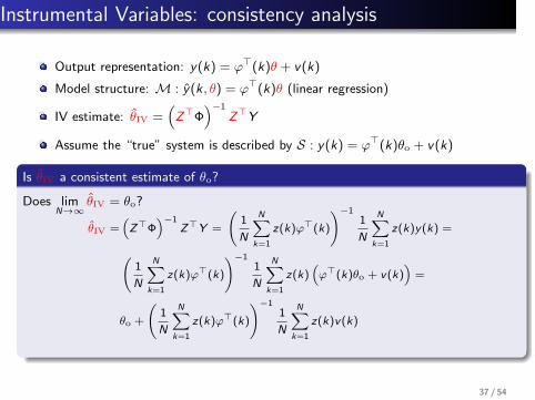

Instrumental Variables: consistency analysis
θIV = θo+
(1
N
N∑k=1
z(k)φ⊤(k)
)−1
1
N
N∑k=1
z(k)v(k)
R(N) =1
N
N∑k=1
z(k)φ⊤(k) is filled out with the estimate of cross covariance
function estimates
Under mild assumptions, limN→∞
R(N) = R∗
z(k) should be correlated with φ(k) (but not with v(k)!) otherwise R(N)
converges to a zero matrix!
limN→∞
1
N
N∑k=1
z(k)v(k) = E [z(k)v(k)] = 0
Thus, θIV is a consistent estimate of θo
38 / 54

Instrumental Variables: how to choose the instruments?
The instrument z(k) should be such that E[z(k)v(k)] = 0
The instrument z(k) should be correlated with φ(k)
In order to minimize the variance of the estimate, we would like to choose:
z(k) = [−yo(k − 1) · · · − yo(k − na) u(k − 1) · · · u(k − nb)]⊤
Summarizing, z(k) should be as much as possible correlated with the noise-freeregressor, but not correlated with the residual v(k).
Choice of the instrument: idea
1 Estimate the model parameters θ through LS (biased estimate!)
2 Perform an open-loop simulation of the estimated model:
y(k) = [−y(k − 1) · · · − y(k − na) u(k − 1) · · · u(k − nb)]⊤ θ
3 Construct the instrument z(k) as follows
z(k) = [−y(k − 1) · · · − y(k − na) u(k − 1) · · · u(k − nb)]⊤
4 Estimate the model parameters θ through IV (consistent estimate)
5 Repeat from step 2 until convergence
39 / 54

Instrumental Variables: how to choose the instruments?
The instrument z(k) should be such that E[z(k)v(k)] = 0
The instrument z(k) should be correlated with φ(k)
In order to minimize the variance of the estimate, we would like to choose:
z(k) = [−yo(k − 1) · · · − yo(k − na) u(k − 1) · · · u(k − nb)]⊤
Summarizing, z(k) should be as much as possible correlated with the noise-freeregressor, but not correlated with the residual v(k).
Choice of the instrument: idea
1 Estimate the model parameters θ through LS (biased estimate!)
2 Perform an open-loop simulation of the estimated model:
y(k) = [−y(k − 1) · · · − y(k − na) u(k − 1) · · · u(k − nb)]⊤ θ
3 Construct the instrument z(k) as follows
z(k) = [−y(k − 1) · · · − y(k − na) u(k − 1) · · · u(k − nb)]⊤
4 Estimate the model parameters θ through IV (consistent estimate)
5 Repeat from step 2 until convergence39 / 54

Prediction Error Methods
40 / 54

Description of Prediction Error Methods
y(k) = G(q, θ)u(k) + H(q, θ)e(k)
E[e(t)e⊤(s)
]= Λeδ(s − t) (i.e., e is white)
G(0, θ) = 0, H(0, θ) = I , H−1(q, θ) is stable
Gu-
y- ev?-
H
e?
+
Linear predictor
y(k|k − 1; θ) = Ly (q−1, θ)y(k) + Lu(q
−1, θ)u(k)Ly (0, θ) = 0, Lu(0, θ) = 0
y(k|k − 1; θ) only depends onpast input/output data
Prediction error
ε(k, θ) = y(k)− y(k|k − 1, θ)
The estimated parameters θ should make the prediction errors {ε(k, θ)}Nk=1 “small”
41 / 54

Description of Prediction Error Methods
Prediction Error Methods
Choice of model structure (parametrization of G(q, θ) and H(q, θ) as a function of θ)
Choice of predictor (define filters of Ly (q−1, θ) and Lu(q−1, θ))
Choice of criterion VN(θ) (scalar function of the prediction errors {ε(k, θ)}Nk=1 to assessthe performance of the predictor)
Estimate the parameters θ = argminθ
VN(θ)
42 / 54

SISO model structures
AutoRegressive with Exogenous inputs (ARX) models
y(k) =B(q, θ)
A(q, θ)u(k) +
1
A(q, θ)e(k)
AutoRegressive-Moving-Average with Exogenous inputs (ARMAX) models
y(k) =B(q, θ)
A(q, θ)u(k) +
C(q, θ)
A(q, θ)e(k)
Output Error (OE) models
y(k) =B(q, θ)
A(q, θ)u(k) + e(k)
Box-Jenkins (BJ) models
y(k) =B(q, θ)
A(q, θ)u(k) +
C(q, θ)
D(q, θ)e(k)
43 / 54

Choice of the predictor filters
Optimal predictor
Choose the prediction filters Ly (q−1, θ) and Lu(q−1, θ) providing the prediction error withsmallest variance
Compute the optimal predictor
y(k) =G(q, θ)u(k) + H(q, θ)e(k) = G(q, θ)u(k) + (H(q, θ)− I ) e(k) + e(k) =
=G(q, θ)u(k) + (H(q, θ)− I )H−1(q, θ) (y(k)− G(q, θ)u(k)) + e(k) =
=[(I − H−1(q, θ)
)y(k) + H−1(q, θ)G(q, θ)u(k)
]+ e(k) =
=z(k) + e(k)
z(k) and e(k) are uncorrelated
Let y∗(k) be an arbitrary predictor of y(k) based on data up to time k − 1
E[(y(k)− y∗(k)) (y(k)− y∗(k))⊤
]= E
[(z(k) + e(k)− y∗(k)) (z(k) + e(k)− y∗(k))⊤
]=
=E[(z(k)− y∗(k)) (z(k)− y∗(k))⊤
]+ E
[e(k)e⊤(k)
]≽ Λe
z(k) is the optimal predictor and e(k) is the “optimal” prediction error
y(k|k − 1, θ) =(I − H−1(q−1, θ)
)y(k) + H−1(q−1, θ)G(q−1, θ)u(k)
ε(k, θ) =e(k) = H−1(q−1, θ)(y(k)− G(q−1, θ)u(k)
)
44 / 54

Choice of the predictor filters
Optimal predictor
Choose the prediction filters Ly (q−1, θ) and Lu(q−1, θ) providing the prediction error withsmallest variance
Compute the optimal predictor
y(k) =G(q, θ)u(k) + H(q, θ)e(k) = G(q, θ)u(k) + (H(q, θ)− I ) e(k) + e(k) =
=G(q, θ)u(k) + (H(q, θ)− I )H−1(q, θ) (y(k)− G(q, θ)u(k)) + e(k) =
=[(I − H−1(q, θ)
)y(k) + H−1(q, θ)G(q, θ)u(k)
]+ e(k) =
=z(k) + e(k) z(k) and e(k) are uncorrelated
Let y∗(k) be an arbitrary predictor of y(k) based on data up to time k − 1
E[(y(k)− y∗(k)) (y(k)− y∗(k))⊤
]= E
[(z(k) + e(k)− y∗(k)) (z(k) + e(k)− y∗(k))⊤
]=
=E[(z(k)− y∗(k)) (z(k)− y∗(k))⊤
]+ E
[e(k)e⊤(k)
]≽ Λe
z(k) is the optimal predictor and e(k) is the “optimal” prediction error
y(k|k − 1, θ) =(I − H−1(q−1, θ)
)y(k) + H−1(q−1, θ)G(q−1, θ)u(k)
ε(k, θ) =e(k) = H−1(q−1, θ)(y(k)− G(q−1, θ)u(k)
)44 / 54

Minimization criterion
Choice of the loss function VN(θ)
Sample covariance matrix
RN(θ) =1
N
N∑k=1
ε(k, θ)ε⊤(k, θ)
If y is scalar, RN(θ) can be taken as the criterion VN(θ) to be minimized
In the multivariable case, we can minimize
VN(θ) = h(RN(θ))
with h continuous monotonically increasing function defined on the set of positivesemidefinite matrices:
h(Q +∆Q) ≥ h(Q) ∀Q,∆Q ≽ 0.
Ex: VN(θ) = h(RN(θ)) = tr (RN(θ))
Final estimate
θPEM = argminθ
VN(θ)
45 / 54

PEM: Asymptotic analysis
What happens when N → ∞?
limN→∞
RN(θ) = E[ε(k, θ)ε⊤(k, θ)
]= R∞(θ)
limN→∞
h (RN(θ)) = h (R∞(θ)) = V∞(θ)
Convergence is uniform on a compact set Θ, i.e.,
supθ∈Θ
|VN(θ)− V∞(θ)| → 0
limN→∞
θPEM = θ∗ = argminθ
V∞(θ)
Is θPEM a consistent estimate of θo?
Let θo be the true system parameters:
y(k) = G(q, θo)u(k) + H(q, θo)e(k), E[e(t)e⊤(s)
]= Λeδ(s − t),
G(0, θo) = 0, H(0, θo) = I , H−1(q, θo) stable
46 / 54

PEM: Asymptotic analysis
Is θPEM a consistent estimate of θo?
Let θo be the true system parameters:
y(k) = G(q, θo)u(k) + H(q, θo)e(k), E[e(t)e⊤(s)
]= Λeδ(s − t),
G(0, θo) = 0, H(0, θo) = I , H−1(q, θo) stable
Thus:
ε(k, θ) =H−1(q, θ) (G(q, θo)u(k) + H(q, θo)e(k)− G(q, θ)u(k)) =
=H−1(q, θ) (G(q, θo)− G(q, θ)) u(k) + H−1(q, θ)H(q, θo)e(k) =
=e(k) + terms independent of e(k)
Thus: R∞(θ) = E[ε(k, θ)ε⊤(k, θ)
]≥ E
[e(k)e⊤(k)
]= Λe
θo is a minimizer of h(R∞(θ)) = V∞.
If u(k) and e(k) are not correlated, only the “true” parameters θo minimizeh(R∞(θ)) = V∞
Thus limN→∞
θPEM = θo.
47 / 54

PEM: examples
y(k|k − 1, θ) =(I − H−1(q−1, θ)
)y(k) + H−1(q−1, θ)G(q−1, θ)u(k)
ε(k, θ) =e(k) = H−1(q−1, θ)(y(k)− G(q−1, θ)u(k)
)Predictor for ARX models
y(k) =B(q−1, θ)
A(q−1, θ)u(k) +
1
A(q−1, θ)e(k), e white
Optimal predictor:
y(k|k − 1, θ) =(I − A(q−1, θ)
)y(k) + B(q−1, θ)u(k)
=− a1y(k − 1)− · · · − anay(k − na) + b1u(k − 1) + · · ·+ bnbu(k − nb) =
=φ⊤(k)θ Linear regression representation
PEM estimate:
θPEM=minθ
N∑k=1
(y(k)− y(k|k − 1, θ))2
=minθ
N∑k=1
(y(k)− φ⊤(k)θ
)2=(Φ⊤Φ
)−1Φ⊤Y
LS method and PEM coincide!
48 / 54

PEM: examples
y(k|k − 1, θ) =(I − H−1(q−1, θ)
)y(k) + H−1(q−1, θ)G(q−1, θ)u(k)
ε(k, θ) =e(k) = H−1(q−1, θ)(y(k)− G(q−1, θ)u(k)
)Predictor for ARX models
y(k) =B(q−1, θ)
A(q−1, θ)u(k) +
1
A(q−1, θ)e(k), e white
Optimal predictor:
y(k|k − 1, θ) =(I − A(q−1, θ)
)y(k) + B(q−1, θ)u(k)
=− a1y(k − 1)− · · · − anay(k − na) + b1u(k − 1) + · · ·+ bnbu(k − nb) =
=φ⊤(k)θ
Linear regression representation
PEM estimate:
θPEM=minθ
N∑k=1
(y(k)− y(k|k − 1, θ))2
=minθ
N∑k=1
(y(k)− φ⊤(k)θ
)2=(Φ⊤Φ
)−1Φ⊤Y
LS method and PEM coincide!
48 / 54

PEM: examples
y(k|k − 1, θ) =(I − H−1(q−1, θ)
)y(k) + H−1(q−1, θ)G(q−1, θ)u(k)
ε(k, θ) =e(k) = H−1(q−1, θ)(y(k)− G(q−1, θ)u(k)
)Predictor for ARX models
y(k) =B(q−1, θ)
A(q−1, θ)u(k) +
1
A(q−1, θ)e(k), e white
Optimal predictor:
y(k|k − 1, θ) =(I − A(q−1, θ)
)y(k) + B(q−1, θ)u(k)
=− a1y(k − 1)− · · · − anay(k − na) + b1u(k − 1) + · · ·+ bnbu(k − nb) =
=φ⊤(k)θ Linear regression representation
PEM estimate:
θPEM=minθ
N∑k=1
(y(k)− y(k|k − 1, θ))2
=minθ
N∑k=1
(y(k)− φ⊤(k)θ
)2=(Φ⊤Φ
)−1Φ⊤Y
LS method and PEM coincide!
48 / 54

PEM: examples
y(k|k − 1, θ) =(I − H−1(q−1, θ)
)y(k) + H−1(q−1, θ)G(q−1, θ)u(k)
ε(k, θ) =e(k) = H−1(q−1, θ)(y(k)− G(q−1, θ)u(k)
)Predictor for ARX models
y(k) =B(q−1, θ)
A(q−1, θ)u(k) +
1
A(q−1, θ)e(k), e white
Optimal predictor:
y(k|k − 1, θ) =(I − A(q−1, θ)
)y(k) + B(q−1, θ)u(k)
=− a1y(k − 1)− · · · − anay(k − na) + b1u(k − 1) + · · ·+ bnbu(k − nb) =
=φ⊤(k)θ Linear regression representation
PEM estimate:
θPEM=minθ
N∑k=1
(y(k)− y(k|k − 1, θ))2 =minθ
N∑k=1
(y(k)− φ⊤(k)θ
)2=(Φ⊤Φ
)−1Φ⊤Y
LS method and PEM coincide!
48 / 54

PEM: examples
y(k|k − 1, θ) =(I − H−1(q−1, θ)
)y(k) + H−1(q−1, θ)G(q−1, θ)u(k)
ε(k, θ) =e(k) = H−1(q−1, θ)(y(k)− G(q−1, θ)u(k)
)Predictor for OE models
y(k) =B(q−1, θ)
A(q−1, θ)u(k) + e(k), e white
Optimal predictor:
y(k|k − 1, θ) =B(q−1, θ)
A(q−1, θ)u(k) =
=− a1y(k − 1|k − 2)− · · · − ana y(k − na|k − na − 1)+
+b1u(k − 1) + · · ·+ bnbu(k − nb) =
=φ⊤(k)θ
φ⊤(k) depends on the noise-free past outputs y(k − i |k − i − 1, θ) =B(q−1, θ)
A(q−1, θ)u(k − i)
49 / 54

PEM: numerical optimization
PEM estimate:
θPEM = argminθ
VN(θ) = argminθ
h
(1
N
N∑k=1
ε(k, θ)ε⊤(k, θ)
)
The solution cannot be always computed analytically
Numerical iterative algorithms for non-convex optimization should be used:
i initialize with an initial estimate θ(0)
ii update: θ(i+1) = f (θ(i)) (the estimate is iteratively refined)iii we would like that the estimate converges to the optimum θPEM:
θ(0) → θ(1) → θ(2) → · · · → θPEM
VN(θ)
θ
50 / 54

PEM: numerical optimization
Gradient method
choose an initial condition θ(0);
iterate(i) line search: choose a positive step size t > 0
(ii) update: θ(i+1) = θ(i) − t∂VN(θ)
∂θ
∣∣∣∣θ=θ(i)
until stopping criterion is satisfied (typically:
∥∥∥∥∂VN(θ)
∂θ
∥∥∥∥ ≤ ϵ)
in case of scalar output, VN(θ)=1
N
N∑k=1
ε2(k, θ) and∂VN(θ)
∂θ=
2
N
N∑k=1
ε(k, θ)∂ε(k, θ)
∂θ
it converges (slowly) to the global optimum if VN(θ) is convex
in case of non-convex VN(θ), convergence to the global minimum is notguaranteed
Exact line search
t = argmint>0
VN
(θ(i) + t∆θ
), with ∆θ = − ∂VN(θ)
∂θ
∣∣∣∣θ=θ(i)
51 / 54
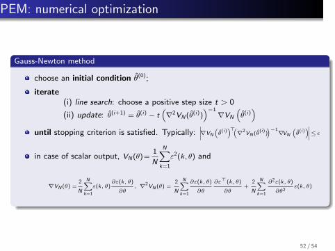
PEM: numerical optimization
Gauss-Newton method
choose an initial condition θ(0);
iterate(i) line search: choose a positive step size t > 0
(ii) update: θ(i+1) = θ(i) − t(∇2VN(θ
(i)))−1
∇VN
(θ(i))
until stopping criterion is satisfied. Typically:∣∣∣∣∇VN
(θ(i)
)⊤(∇2VN (θ(i))
)−1∇VN
(θ(i)
)∣∣∣∣≤ϵ
in case of scalar output, VN(θ)=1
N
N∑k=1
ε2(k, θ) and
∇VN (θ) =2
N
N∑k=1
ε(k, θ)∂ε(k, θ)
∂θ, ∇2VN (θ) =
2
N
N∑k=1
∂ε(k, θ)
∂θ
∂ε⊤(k, θ)
∂θ+
2
N
N∑k=1
∂2ε(k, θ)
∂θ2ε(k, θ)
52 / 54

PEM: numerical optimization
θ(i+1) = θ(i)+t∆θ, with ∆θ = −(∇2VN(θ
(i)))−1
∇VN
(θ(i))
Gauss-Newton method: interpretation
θ(i+1) = θ(i) +∆θ minimizes the second order approximation:
VN (θ(i) + ∆θ) = VN (θ(i)) + ∇VN (θ(i))⊤∆θ +1
2∆θ
⊤∇2VN (θ(i))∆θ
The minimum of the quadratic function above is achieved at ∆θ=−(∇2VN (θ(i))
)−1∇VN
(θ(i))
VN(θ)
θ
(θ(i), VN (θ(i)))VN
VN
(θ(i)+∆θ, VN (θ(i)+∆θ))
Careful: if the Hessian is not positive definite, we move to the “wrong” direction
Hessian approximation:
∇2VN (θ) =2
N
N∑k=1
∂ε(k, θ)
∂θ
∂ε⊤(k, θ)
∂θ+
2
N
N∑k=1
∂2ε(k, θ)
∂θ2ε(k, θ) ≈
2
N
N∑k=1
∂ε(k, θ)
∂θ
∂ε⊤(k, θ)
∂θ+ δI︸︷︷︸regularization
≻0
53 / 54

PEM: numerical optimization
Example: evaluation of the gradient for ARMAX models
ARMAX model: y(k) =B(q−1, θ)
A(q−1, θ)u(k) +
C(q−1, θ)
A(q−1, θ)e(k)
prediction error ε(k, θ) : C(q−1, θ)ε(k, θ) = A(q−1, θ)y(k)− B(q−1, θ)u(k)
compute derivatives of both left and right hand of the above equation:
C(q−1, θ)∂ε(k, θ)
∂ai= y(k − i) ⇒
∂ε(k, θ)
∂ai=
1
C(q−1, θ)y(k − i)
C(q−1, θ)∂ε(k, θ)
∂bi= −u(k − i) ⇒
∂ε(k, θ)
∂bi= −
1
C(q−1, θ)u(k − i)
ε(k − i , θ) + C(q−1, θ)∂ε(k, θ)
∂ci= 0 ⇒
∂ε(k, θ)
∂ci= −
1
C(q−1, θ)ε(k − i , θ)
Thus:
∂ε(k, θ)
∂θ=[yF (k−1) · · · yF (k−na) −uF (k− 1) · · · −uF (k−nb) −εF (k−1) · · · −εF (k−nc)]
⊤
with:
yF (k) =1
C(q−1, θ)y(k), uF (k) =
1
C(q−1, θ)u(k), εF (k) =
1
C(q−1, θ)ε(k)
54 / 54


![Lecture Two: The Analogy Theory [‘AT’] · Lecture Two: The Analogy Theory ... 2. [AT] claims: OM-judgments justified by an argument from analogy ... iPaul Bartha, “Analogy and](https://img.pdfslide.us/doc/110x75/5b1ae5387f8b9a28258e143b/lecture-two-the-analogy-theory-at-lecture-two-the-analogy-theory-.jpg)