Efficient Computation of Persistent Homologyfor Cubical Data

Hubert Wagner, Chao Chen, Erald Vucini

Abstract In this paper we present an efficient framework for computation of persis-tent homology of cubical data in arbitrary dimensions. An existing algorithm usingsimplicial complexes is adapted to the setting of cubical complexes. The proposedapproach enables efficient application of persistent homology in domains where thedata is naturally given in a cubical form. By avoiding triangulation of the data, wesignificantly reduce the size of the complex. We also presenta data-structure de-signed to compactly store and quickly manipulate cubical complexes. By meansof numerical experiments, we show high speed and memory efficiency of our ap-proach. We compare our framework to other available implementations, showing itssuperiority. Finally, we report performance on selected 3Dand 4D data-sets.

1 Introduction

Persistent homology [10, 11] has drawn much attention in visualization and dataanalysis, mainly due to the fact that it extracts topological information that is re-silient to noise. This is especially important in application areas, where data typi-cally comes from measurements which are inherently inexact. Although direct ap-

Hubert WagnerVienna University of Technology, Austria andJagiellonian University, Polande-mail: hubert.wagner@ii.uj.edu.pl

Chao ChenInstitute of Science and Technology Austria andVienna University of Technology, Austriae-mail: chao.chen@ist.ac.at

Erald VuciniVRVis Center for Virtual Reality and Visualization Research-Ltd, Austria andVienna University of Technology, Austriae-mail: erald.vucini@vrvis.at

1

2 Hubert Wagner, Chao Chen, Erald Vucini

plication of persistent homology is still at an early stage,closely related conceptslike size functions [4], contour trees [2, 5], Reeb graphs [24] and Morse-Smale com-plexes [14] have been successfully used.

The under-usage of persistence in applications is largely due to its high compu-tational cost. The standard algorithm [10] takes cubic running time, which can beprohibitive even for small size data (e.g., 64×64×64). In addition to the high timecomplexity, there are two further issues:(1) the memory consumption of the cur-rently available implementations, even for small data sizes, is very large and henceprohibitive for commodity computers, and(2) the focus of several applications is indata of higher dimensions, e.g., 4D, 5D or higher. Few implementations for generaldimension are available and the existing ones do not scale well with the increase ofdimensions, hence introducing larger computational timesand memory inefficiency.

In this paper, we present an efficient framework that computes persistent homol-ogy exactly1. To our knowledge, this is the very first implementation thatcouldhandle large size and high dimensional data in reasonable time and memory. We fo-cus on uniformly/regularly sampled data which is common in visualization and dataanalysis, i.e. image data consisting of pixels (2D images),voxels (3D scans, simula-tions), or their higher-dimensional analogs, e.g., 4D time-varying data. In this work,we use the name ’cubical’ for such data.

We depart from the standard method which involves triangulating the space, andcomputing persistent homology of the resulting simplicialcomplex [10, 11]. We usecubical complexes [15], which do not require subdivision ofthe input. The advan-tage is twofold. First, the size of the complexes is significantly reduced, especiallyfor high dimensional data (see Section 5 for a quantitative analysis). Second, cubicalcomplexes allow the usage of more compact data-structures.

The standard persistence algorithm requires the computation of a sorted bound-ary matrix. This step can be a significant bottleneck, especially in terms of memoryconsumption. In this work we provide an efficient and compactalgorithm for thisstep, using techniques from (non-persistence) cubical homology [15] (see Section4).

Finally, in Section 7, we present experimental results. Comparison with exist-ing packages shows significant efficiency improvement. We also explore how ourmethod scales with respect to data size and dimension. In conclusion, our frame-work can handle data of large size and high dimension, and therefore, makes thepersistence computation of cubical data more feasible.

2 Related Work

The first algorithm for computing persistence [11] has cubicrunning time with re-gard to the complex size (which is larger than the input size). Morozov [20] formu-lated a worst case scenario for which the persistence algorithm reaches this asymp-

1 We emphasize that our work focuses on computing persistenceexactly. There are approximationmethods which trade accuracy for efficiency. See Section 2.

Cubical Persistence 3

totic bound. When focusing on 0-dimensional homology, union-find data structurescan be used to compute persistence in timeO(nα(n)) [10], whereα is the inverse ofthe Ackermann functions andn is the input size. Milosavljevic et al. [18] computepersistent homology in matrix multiplication timeO(nω) where the currently bestestimation ofω is 2.376. Chen and Kerber [6] proposed a randomized algorithmwhose complexity depends on the number of persistence pairswhose persistence isover a certain threshold. Despite showing better theoretical complexity, it is unclearwhether these methods are better than the standard persistence algorithm in practice.

In terms of implementation, Morozov [19] provides a C++ codefor the persis-tence algorithm. Chen and Kerber [7] devised a technique which, in practice, sig-nificantly improves the matrix-reduction part of this algorithm. We build upon theirwork, to improve the overall performance of the persistencealgorithm.

The application of cubical homology is straightforward in the areas of imageprocessing and visualization, where cubical data is the typical input. Non-persistentcubical homology has found practical applications in a number of cases [21, 22]. Afew attempts of cubical persistence computations have beenmade recently [16, 25].They do not, however, tackle the problem of performance. In [25], experiments withdatasets containing several thousands of voxels are reported. In comparison, realworld applications require processing of data in the range of millions or billions ofvoxels.

Recently, Mrozek and Wanner [21] showed that cubical persistent homology canbe used for medium-sized datasets. A detailed performance summary is given for 2Dand 3D images. One downside of this approach is the dependency on the numberof unique values of the image. When such number is close to theinput size, thecomplexity is prohibitively high. In Section 7, we compare our method with thisalgorithm.

We must differentiate between two main types of persistencecomputations: exactand approximative (where the persistence is calculated approximately). While wefocus on the first type, approximation is less computationally intensive, and thus isimportant for large data. Bendich et al. [3] use octrees to approximate the input. Asimplicial complex of small size is then used to complete persistence computation.

3 Theoretical Background

Simplicial and cubical complexes. In computational topology, simplicial com-plexes are frequently used to describe topological spaces.A simplicial complexconsists of simplices like vertices, edges and triangles. In general, ad-simplexisthe convex hull ofd+1 points. The convex hull of any subset of thesed+1 pointsis a faceof this d-simplex. A collection of simplices,K, is asimplicial complexif:1) for any simplex inK, all its faces also belong toK, and 2) for any two simplicesin K, their intersection is either empty, or a common face of them.

Next, we define cubical complexes. Anelementary intervalis defined as a unitinterval [k,k+1], or a degenerate interval[k,k]. For ad-dimensional space, acube

4 Hubert Wagner, Chao Chen, Erald Vucini

(a) (b) (c) (d)

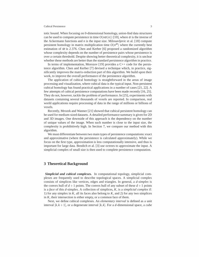
Fig. 1 Cubical complex triangulations: a) a 2D cubical complex, and b) its triangulation, c) a 3Dcubical complex, and d) its triangulation (only simplices which containV0 are drawn).

is a product ofd elementary intervalsI : ∏di=1 Ii. The number of non-degenerate

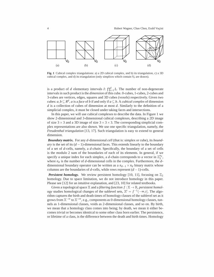
intervals in such product is thedimensionof this cube. 0-cubes, 1-cubes, 2-cubes and3-cubes are vertices, edges, squares and 3D cubes (voxels) respectively. Given twocubes:a,b⊆Rd, a is afaceof b if and only ifa⊆ b. A cubical complexof dimensiond is a collection of cubes of dimension at mostd. Similarly to the definition of asimplicial complex, it must be closed under taking faces andintersections.

In this paper, we will use cubical complexes to describe the data. In Figure 1 weshow 2-dimensional and 3-dimensional cubical complexes, describing a 2D imageof size 3×3 and a 3D image of size 3×3×3. The corresponding simplicial com-plex representations are also shown. We use one specific triangulation, namely, theFreudenthal triangulation[13, 17]. Such triangulation is easy to extend to generaldimension.

Boundary matrix. For anyd-dimensionalcell (that is: simplex or cube), itsbound-ary is the set of its (d−1)-dimensional faces. This extends linearly to the boundaryof a set ofd-cells, namely, ad-chain. Specifically, the boundary of a set of cellsis the modulo 2 sum of the boundaries of each of its elements. In general, if wespecify a unique index for each simplex, ad-chain corresponds to a vector inZnd

2 ,wherend is the number ofd-dimensional cells in the complex. Furthermore, thed-dimensional boundary operator can be written as and−1×nd binary matrix whosecolumns are the boundaries ofd-cells, while rows represent (d−1)-cells.

Persistent homology. We review persistent homology [10, 11], focusing onZ2

homology. Due to space limitation, we do not introduce homology in this paper.Please see [12] for an intuitive explanation, and [23, 10] for related textbooks.

Given a topological spaceX and afiltering function f:X→R, persistent homol-ogystudies homological changes of the sublevel sets,X

t = f−1(−∞, t]. The algo-rithm captures the birth and death times of homology classesof the sublevel set as itgrows fromX

−∞ toX+∞, e.g., components as 0-dimensional homology classes, tun-

nels as 1-dimensional classes, voids as 2-dimensional classes, and so on. By birth,we mean that a homology class comes into being; by death, we mean it either be-comes trivial or becomes identical to some other class born earlier. The persistence,or lifetime of a class, is the difference between the death and birth times. Homology

Cubical Persistence 5

classes with larger persistence reveal information about the global structure of thespaceX, as described by the functionf .

Persistence could be visualized in different ways. One well-accepted idea is thepersistence diagram [8], which is a set of points in a two-dimensional plane, eachcorresponding to a persistent homology class. The coordinates of such a point arethe birth and death time of the related class.

An important justification of the usage of persistence is thestability theorem.Cohen-Steiner et al. [8] proved that for any two filtering functions f and g, thedifference of their persistence is always upperbounded by theL∞ norm of their dif-ference:

‖ f −g‖∞ := maxx∈X| f (x)−g(x)|.

This guarantees that persistence can be used as a signature.Whenever two persis-tence outputs are different, we know that the functions are definitely different.

In our framework, for 2D images we assume 4-connectivity. Ingeneral, ford-dimensional cubical data, we use 2d-connectivity.

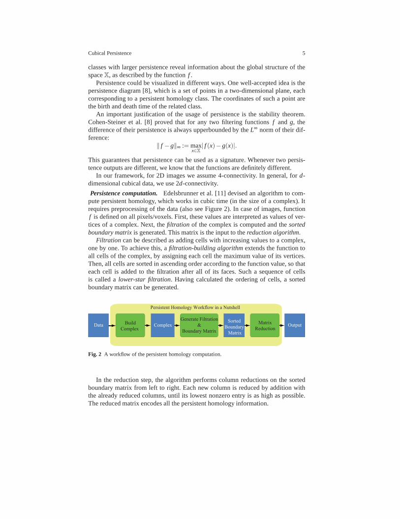
Persistence computation. Edelsbrunner et al. [11] devised an algorithm to com-pute persistent homology, which works in cubic time (in the size of a complex). Itrequires preprocessing of the data (also see Figure 2). In case of images, functionf is defined on all pixels/voxels. First, these values are interpreted as values of ver-tices of a complex. Next, thefiltration of the complex is computed and thesortedboundary matrixis generated. This matrix is the input to thereduction algorithm.

Filtration can be described as adding cells with increasing values to a complex,one by one. To achieve this, afiltration-building algorithmextends the function toall cells of the complex, by assigning each cell the maximum value of its vertices.Then, all cells are sorted in ascending order according to the function value, so thateach cell is added to the filtration after all of its faces. Such a sequence of cellsis called alower-star filtration. Having calculated the ordering of cells, a sortedboundary matrix can be generated.

Data Build

Complex

Matrix

ReductionOutput

Persistent Homology Workflow in a Nutshell

ComplexSorted

Boundary

Matrix

Generate Filtration

&

Boundary Matrix

Fig. 2 A workflow of the persistent homology computation.

In the reduction step, the algorithm performs column reductions on the sortedboundary matrix from left to right. Each new column is reduced by addition withthe already reduced columns, until its lowest nonzero entryis as high as possible.The reduced matrix encodes all the persistent homology information.

6 Hubert Wagner, Chao Chen, Erald Vucini

4 Efficient Filtration-Building Algorithm

The filtration-building is one of the main bottlenecks of thepersistence algorithm. Astraightforward approach would choose to store the boundary relationship betweencells and their faces. In this section, we describe the first major contribution of thepaper, a new algorithm for the filtration-building step. Ouralgorithm uses the regularstructure of cubical complex and adapts a compact data structure which has shownits power in non-persistent cubical homology.

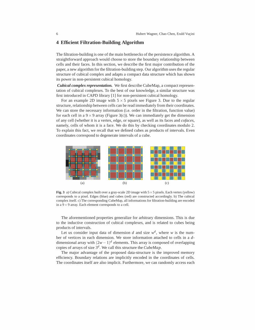
Cubical complex representation. We first describe CubeMap, a compact represen-tation of cubical complexes. To the best of our knowledge, a similar structure wasfirst introduced in CAPD library [1] for non-persistent cubical homology.

For an example 2D image with 5× 5 pixels see Figure 3. Due to the regularstructure, relationship between cells can be read immediately from their coordinates.We can store the necessary information (i.e. order in the filtration, function value)for each cell in a 9×9 array (Figure 3(c)). We can immediately get the dimensionof any cell (whether it is a vertex, edge, or square), as well as its faces andcofaces,namely, cells of whom it is a face. We do this by checking coordinates modulo 2.To explain this fact, we recall that we defined cubes as products of intervals. Evencoordinates correspond to degenerate intervals of a cube.

(a) (b) (c)

Fig. 3 a) Cubical complex built over a gray-scale 2D image with 5×5 pixels. Each vertex (yellow)corresponds to a pixel. Edges (blue) and cubes (red) are constructed accordingly. b) The cubicalcomplex itself. c) The corresponding CubeMap, all informations for filtration-building are encodedin a 9×9 array. Each element corresponds to a cell.

The aforementioned properties generalize for arbitrary dimensions. This is dueto the inductive construction of cubical complexes, and is related to cubes beingproducts of intervals.

Let us consider input data of dimensiond and sizewd, wherew is the num-ber of vertices in each dimension. We store information attached to cells in ad-dimensional array with(2w−1)d elements. This array is composed of overlappingcopies of arrays of size 3d. We call this structure theCubeMap.

The major advantage of the proposed data-structure is the improved memoryefficiency. Boundary relations are implicitly encoded in the coordinates of cells.The coordinates itself are also implicit. Furthermore, we can randomly access each

Cubical Persistence 7

5 3

2

5

3

2

5 5

1

(a)

V(0) E(0) V(1)

V(3) V(2)

E(2) S(0) E(1)

E(3)

(b)

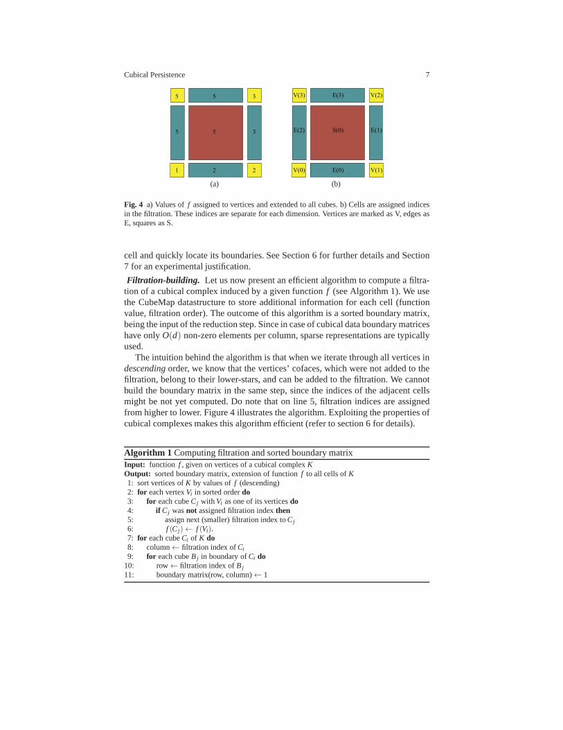
Fig. 4 a) Values off assigned to vertices and extended to all cubes. b) Cells are assigned indicesin the filtration. These indices are separate for each dimension. Vertices are marked as V, edges asE, squares as S.

cell and quickly locate its boundaries. See Section 6 for further details and Section7 for an experimental justification.

Filtration-building. Let us now present an efficient algorithm to compute a filtra-tion of a cubical complex induced by a given functionf (see Algorithm 1). We usethe CubeMap datastructure to store additional informationfor each cell (functionvalue, filtration order). The outcome of this algorithm is a sorted boundary matrix,being the input of the reduction step. Since in case of cubical data boundary matriceshave onlyO(d) non-zero elements per column, sparse representations are typicallyused.

The intuition behind the algorithm is that when we iterate through all vertices indescendingorder, we know that the vertices’ cofaces, which were not added to thefiltration, belong to their lower-stars, and can be added to the filtration. We cannotbuild the boundary matrix in the same step, since the indicesof the adjacent cellsmight be not yet computed. Do note that on line 5, filtration indices are assignedfrom higher to lower. Figure 4 illustrates the algorithm. Exploiting the properties ofcubical complexes makes this algorithm efficient (refer to section 6 for details).

Algorithm 1 Computing filtration and sorted boundary matrixInput: function f , given on vertices of a cubical complexKOutput: sorted boundary matrix, extension of functionf to all cells ofK1: sort vertices ofK by values off (descending)2: for each vertexVi in sorted orderdo3: for each cubeCj with Vi as one of its verticesdo4: if Cj wasnot assigned filtration indexthen5: assign next (smaller) filtration index toCj

6: f (Cj )← f (Vi).7: for each cubeCi of K do8: column← filtration index ofCi

9: for each cubeB j in boundary ofCi do10: row← filtration index ofB j

11: boundary matrix(row, column)← 1

8 Hubert Wagner, Chao Chen, Erald Vucini

5 Sizes of Complexes

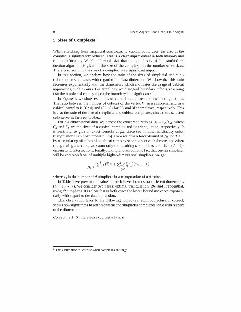
When switching from simplicial complexes to cubical complexes, the size of thecomplex is significantly reduced. This is a clear improvement in both memory andruntime efficiency. We should emphasize that the complexityof the standard re-duction algorithm is given in the size of the complex, not thenumber of vertices.Therefore, reducing the size of a complex has a significant impact.

In this section, we analyze how the ratio of the sizes of simplicial and cubi-cal complexes increases with regard to the data dimension. We show that this ratioincreases exponentially with the dimension, which motivates the usage of cubicalapproaches, such as ours. For simplicity we disregard boundary effects, assumingthat the number of cells lying on the boundary is insignificant2.

In Figure 1, we show examples of cubical complexes and their triangulations.The ratio between the number of cofaces of the vertexV0 in a simplicial and in acubical complex is(6 : 4) and(26 : 8) for 2D and 3D complexes, respectively. Thisis also the ratio of the size of simplicial and cubical complexes, since these selectedcells serve as theirgenerators.

For ad-dimensional data, we denote the concerned ratio asρd = Sd/Cd, whereCd andSd are the sizes of a cubical complex and its triangulation, respectively. Itis nontrivial to give an exact formula ofρd, since the minimal-cardinality cube-triangulation is an open problem [26]. Here we give a lower-bound ofρd for d≤ 7by triangulating all cubes of a cubical complex separately in each dimension. Whentriangulating ad-cube, we count only the resultingd-simplices, and their(d−1)-dimensional intersections. Finally, taking into account the fact that certain simpliceswill be common faces of multiple higher-dimensional simplices, we get

ρd ≥∑d

i=0

(di

)

τi +∑d−1i=0

( di+1

)

(τi+1−1)

2d

whereτd is the number ofd-simplices in a triangulation of ad-cube.In Table 1 we present the values of such lower-bounds for different dimensions

(d = 1, · · · ,7). We consider two cases: optimal triangulation [26] and Freudenthal,usingd! simplices. It is clear that in both cases the lower-bound increases exponen-tially with regard to the data dimension.

This observation leads to the following conjecture. Such conjecture, if correct,shows how algorithms based on cubical and simplicial complexes scale with respectto the dimension.

Conjecture 1.ρd increases exponentially ind.

2 This assumption is realistic when complexes are large.

Cubical Persistence 9

Table 1 Lower-bounds of the size ratiosρd.

Dimension (d) 1 2 3 4 5 6 7

Optimalτd 1 2 5 16 67 308 1493lower-bound ofρd 1.0 1.5 2.75 5.62512.93733.968 90.265

Freudenthalτd 1 2 6 24 120 720 5040lower-bound ofρd 1.0 1.5 3.0 7.12519.37560.156213.062

6 Implementation Details

In this section we briefly comment on the techniques we used toenhance the perfor-mance of our implementation. We focus on the choice of properdata-structures, andexploiting various features of cubical complexes. We implemented this algorithm inC++.

Filtration-building algorithm. We use a 2-pass modification of the standardfiltration-building algorithm. Reversing the iteration order over the vertices doesnot affect the asymptotic complexity, but simplifies the first pass of the algorithm,which resulted in better performance.

We calculate the time complexity of this algorithm. To do this precisely, we as-sume that the dimensiond is not a constant. This is a fair assumption since weconsider general dimensions. We use ad-dimensional array to store our data, sorandom access is notO(1), butO(d), as it takesd−1 multiplications and additionsto calculate the address in memory.

Let n be the size of input (the number of vertices in our complex). In total thereare O(2dn) cubes in the complex. We ignore what happens at boundaries ofthecomplex. Eachd-cube has exactly 2d boundary cubes, and each vertex has 3d−1cofaces. Accessing each of them costsO(d). This yields the following complexityof calculating the filtration and the boundary matrices:O(d3dn+d22dn).

Using the properties of CubeMap, we can reduce this complexity. Since the struc-ture of the whole complex is regular, we can precalculate memory-offsets fromcubes of different dimensions and orientations to its cofaces and boundaries. Ac-cessing all boundary cubes and cofaces takes constant amortized time. The pre-processing time does not depend on input size and takes onlyO(d23d) time andmemory. With the CubeMap data structure, our algorithm can be implemented inΘ(3dn+d2dn) time andΘ(d2dn) memory.

Storing boundary matrices. Now we present a suggestion regarding performance,namely, the usage of a proper data-structure for storing thecolumns of (sparse)boundary matrices. In [10] a linked-list data-structure issuggested. This seems tobe a sub-optimal solution, as it has an overhead of at least one pointer per storedelement. For 64-bit machines this is 8B - twice as much as the data we need to storein a typical situation (one 32-bit integer).

Using an automatically-growing array, such as std::vectoravailable in STL ismuch more efficient (speed-up by a factor of at least 2). Also the memory over-head is much smaller - 16B per column (not per element as before). All the required

10 Hubert Wagner, Chao Chen, Erald Vucini

operations have the same (amortized) complexity [9], assuming that adding an ele-ment at the back can be done in constant amortized time. Also,iterating the arrayfrom left to right is fast, due to memory-locality, which is not the case for linked-listimplementations.

7 Results

The testing platform of our experiments is a six-core AMD Opteron(tm) processor2.4GHz with 512KB L2 cache per core, and 66GB of RAM, running Linux. Our al-gorithm runs on a single core. We use 3D and 4D (3D+time) cubical data for testingand comparing our algorithm. We compare our method with existing implementa-tions. We measure memory usage, filtration-building and reduction times.

Comparing with existing implementations. We compare our implementation (re-ferred to as CubPers) to three existing implementations:

1. SimpPers:(by Chen and Kerber [7]) Uses simplicial complexes. Both SimpPersand CubPers use the same reduction algorithm, but our approach uses cubicalcomplexes and CubeMap to accelerate the filtration-building process.

2. Dionysus: (by Morozov [19]) This code is suited for more general complexesand computes also other information like vineyards. We adapt this implementa-tion to operate on cubical data, by triangulating the input,which is the standardapproach. Since this implementation takes a filtration as input, the time for build-ing the filtration is not taken into account.

3. CAPD: (by Mrozek [21], a part of CAPD library [1]) We stress that this approachwas designed for data with a small number of unique function values, which isnot the case for the data we use. Additionally it produces andstores persistenthomology generators which incur a significant overhead.

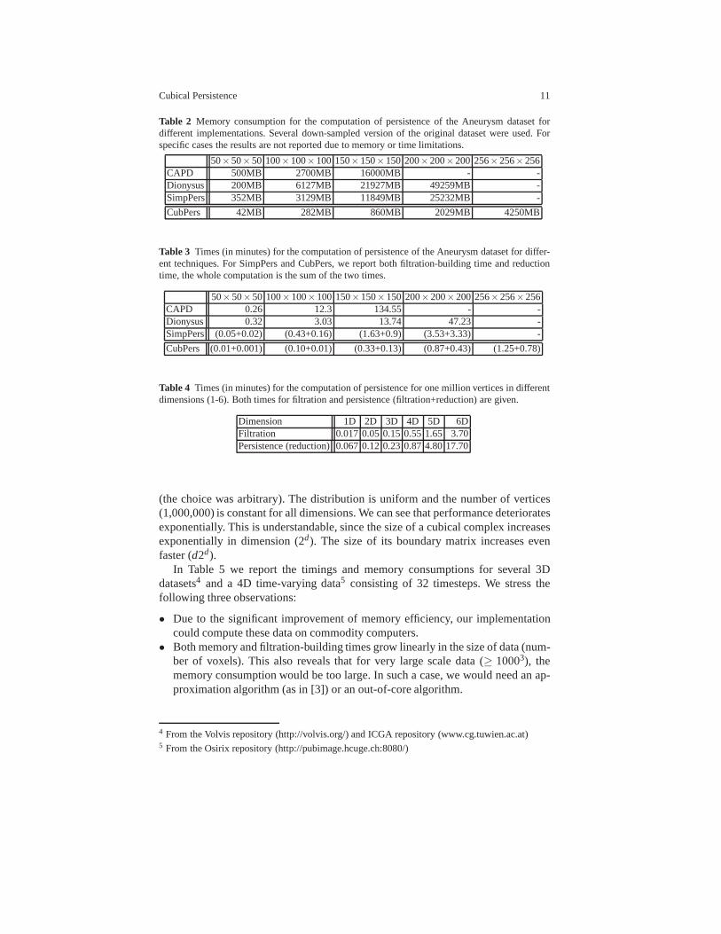
In Tables 2 and 3 we compare the memory and times of our approach to theaforementioned implementations. For testing we have used the Aneurysm dataset3.In order to explore the behavior of the algorithms when the data size increases lin-early, we uniformly scale the data into 503, 1003, 1503, 2003, using nearest neighborinterpolation. Clearly, our implementation, CubPers, outperforms other programs interms of memory and time efficiency.

Due to the usage of CubeMap, the memory usage is reduced by an order ofmagnitude. This is extremely important, as it enables the usage of much larger data-sets on commodity computers. While SimpPers significantly improves over othermethods in terms of reduction time [7], our method further improves the filtration-building time. It is also shown that using cubical complexesinstead of simplicialcomplexes improves the reduction time.

Scalability. Table 4 shows how our implementation scales with respect to dimen-sion. We used random data - each vertex is assigned an integervalue from 0 to 1023

3 From the Volvis repository (http://volvis.org/).

Cubical Persistence 11

Table 2 Memory consumption for the computation of persistence of the Aneurysm dataset fordifferent implementations. Several down-sampled versionof the original dataset were used. Forspecific cases the results are not reported due to memory or time limitations.

50×50×50 100×100×100 150×150×150 200×200×200 256×256×256CAPD 500MB 2700MB 16000MB - -Dionysus 200MB 6127MB 21927MB 49259MB -SimpPers 352MB 3129MB 11849MB 25232MB -

CubPers 42MB 282MB 860MB 2029MB 4250MB

Table 3 Times (in minutes) for the computation of persistence of theAneurysm dataset for differ-ent techniques. For SimpPers and CubPers, we report both filtration-building time and reductiontime, the whole computation is the sum of the two times.

50×50×50 100×100×100 150×150×150 200×200×200 256×256×256CAPD 0.26 12.3 134.55 - -Dionysus 0.32 3.03 13.74 47.23 -SimpPers (0.05+0.02) (0.43+0.16) (1.63+0.9) (3.53+3.33) -

CubPers (0.01+0.001) (0.10+0.01) (0.33+0.13) (0.87+0.43) (1.25+0.78)

Table 4 Times (in minutes) for the computation of persistence for one million vertices in differentdimensions (1-6). Both times for filtration and persistence(filtration+reduction) are given.

Dimension 1D 2D 3D 4D 5D 6DFiltration 0.0170.05 0.15 0.55 1.65 3.70Persistence (reduction)0.0670.12 0.23 0.87 4.80 17.70

(the choice was arbitrary). The distribution is uniform andthe number of vertices(1,000,000) is constant for all dimensions. We can see that performance deterioratesexponentially. This is understandable, since the size of a cubical complex increasesexponentially in dimension (2d). The size of its boundary matrix increases evenfaster (d2d).

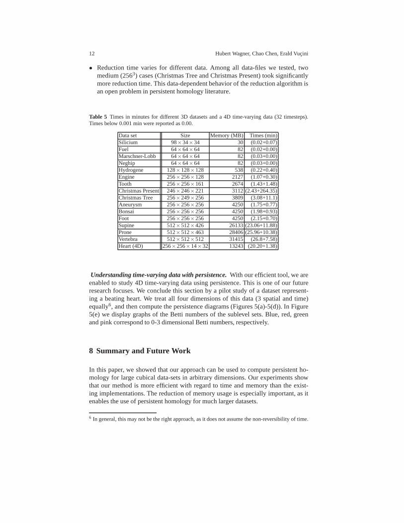
In Table 5 we report the timings and memory consumptions for several 3Ddatasets4 and a 4D time-varying data5 consisting of 32 timesteps. We stress thefollowing three observations:

• Due to the significant improvement of memory efficiency, our implementationcould compute these data on commodity computers.

• Both memory and filtration-building times grow linearly in the size of data (num-ber of voxels). This also reveals that for very large scale data (≥ 10003), thememory consumption would be too large. In such a case, we would need an ap-proximation algorithm (as in [3]) or an out-of-core algorithm.

4 From the Volvis repository (http://volvis.org/) and ICGA repository (www.cg.tuwien.ac.at)5 From the Osirix repository (http://pubimage.hcuge.ch:8080/)

12 Hubert Wagner, Chao Chen, Erald Vucini

• Reduction time varies for different data. Among all data-files we tested, twomedium (2563) cases (Christmas Tree and Christmas Present) took significantlymore reduction time. This data-dependent behavior of the reduction algorithm isan open problem in persistent homology literature.

Table 5 Times in minutes for different 3D datasets and a 4D time-varying data (32 timesteps).Times below 0.001 min were reported as 0.00.

Data set Size Memory (MB) Times (min)Silicium 98×34×34 30 (0.02+0.07)Fuel 64×64×64 82 (0.02+0.00)Marschner-Lobb 64×64×64 82 (0.03+0.00)Neghip 64×64×64 82 (0.03+0.00)Hydrogene 128×128×128 538 (0.22+0.40)Engine 256×256×128 2127 (1.07+0.30)Tooth 256×256×161 2674 (1.43+1.48)Christmas Present 246×246×221 3112 (2.43+264.35)Christmas Tree 256×249×256 3809 (3.08+11.1)Aneurysm 256×256×256 4250 (1.75+0.77)Bonsai 256×256×256 4250 (1.98+0.93)Foot 256×256×256 4250 (2.15+0.70)Supine 512×512×426 26133(23.06+11.88)Prone 512×512×463 28406(25.96+10.38)Vertebra 512×512×512 31415 (26.8+7.58)Heart (4D) 256×256×14×32 13243 (20.20+1.38)

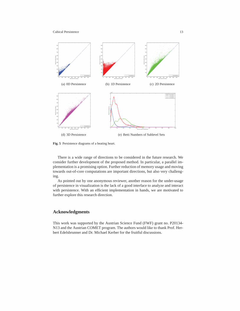
Understanding time-varying data with persistence. With our efficient tool, we areenabled to study 4D time-varying data using persistence. This is one of our futureresearch focuses. We conclude this section by a pilot study of a dataset represent-ing a beating heart. We treat all four dimensions of this data(3 spatial and time)equally6, and then compute the persistence diagrams (Figures 5(a)-5(d)). In Figure5(e) we display graphs of the Betti numbers of the sublevel sets. Blue, red, greenand pink correspond to 0-3 dimensional Betti numbers, respectively.

8 Summary and Future Work

In this paper, we showed that our approach can be used to compute persistent ho-mology for large cubical data-sets in arbitrary dimensions. Our experiments showthat our method is more efficient with regard to time and memory than the exist-ing implementations. The reduction of memory usage is especially important, as itenables the use of persistent homology for much larger datasets.

6 In general, this may not be the right approach, as it does not assume the non-reversibility of time.

Cubical Persistence 13

0 100 200 300 400 500 600 700 800 900

0

100

200

300

400

500

600

700

800

900

Birth (Function Value)

De

ath

(F

un

ctio

n V

alu

e)

0−persistence

(a) 0D Persistence

0 100 200 300 400 500 600 700 800 900

0

100

200

300

400

500

600

700

800

900

Birth (Function Value)

De

ath

(F

un

ctio

n V

alu

e)

1−persistence

(b) 1D Persistence

0 100 200 300 400 500 600 700 800 900

0

100

200

300

400

500

600

700

800

900

Birth (Function Value)

De

ath

(F

un

ctio

n V

alu

e)

2−persistence

(c) 2D Persistence

0 100 200 300 400 500 600 700 800 900

0

100

200

300

400

500

600

700

800

900

Birth (Function Value)

De

ath

(F

un

ctio

n V

alu

e)

3−persistence

(d) 3D Persistence

0 100 200 300 400 500 600 700 800 900 10000

1

2

3

4

5

6x 10

4

Function Value [0, MaxValue]

Pe

rsis

ten

ce F

req

ue

ncy

0−persistence

1−persistence

2−persistence

3−persistence

(e) Betti Numbers of Sublevel Sets

Fig. 5 Persistence diagrams of a beating heart.

There is a wide range of directions to be considered in the future research. Weconsider further development of the proposed method. In particular, a parallel im-plementation is a promising option. Further reduction of memory usage and movingtowards out-of-core computations are important directions, but also very challeng-ing.

As pointed out by one anonymous reviewer, another reason forthe under-usageof persistence in visualization is the lack of a good interface to analyze and interactwith persistence. With an efficient implementation in hands, we are motivated tofurther explore this research direction.

Acknowledgments

This work was supported by the Austrian Science Fund (FWF) grant no. P20134-N13 and the Austrian COMET program. The authors would like tothank Prof. Her-bert Edelsbrunner and Dr. Michael Kerber for the fruitful discussions.

14 Hubert Wagner, Chao Chen, Erald Vucini

References

1. Computer Assisted Proofs in Dynamics: CAPD Homology Library, http://capd.ii.uj.edu.pl.2. C. L. Bajaj, V. Pascucci, and D. Schikore. The contour spectrum. In Proceedings of IEEE

Visualization, pages 167–174, 1997.3. P. Bendich, H. Edelsbrunner, and M. Kerber. Computing robustness and persistence for im-

ages. InProceedings of IEEE Visualization, volume 16, pages 1251–1260, 2010.4. S. Biasotti, A. Cerri, P. Frosini, D. Giorgi, and C. Landi.Multidimensional size functions for

shape comparison.J. Math. Imaging Vis., 32(2):161–179, 2008.5. H. Carr, J. Snoeyink, and M. van de Panne. Flexible isosurfaces: Simplifying and displaying

scalar topology using the contour tree.Computational Geometry, 43(1):42–58, 2010.6. C. Chen and M. Kerber. An Output-Sensitive Algorithm for Persistent Homology. InPro-

ceedings of the 27th annual symposium on Computational geometry, 2011.7. C. Chen and M. Kerber. Persistent homology computation with a twist. In27th European

Workshop on Computational Geometry (EuroCG 2011), 2011.8. D. Cohen-Steiner, H. Edelsbrunner, and J. Harer. Stability of persistence diagrams.Discrete

and Computational Geometry, 37(1):103–120, 2007.9. T. H. Cormen, C. E. Leiserson, R. L. Rivest, and C. Stein.Introduction to algorithms. The

MIT press, 2009.10. H. Edelsbrunner and J. Harer.Computational Topology, An Introduction.American Mathe-

matical Society, 2010.11. H. Edelsbrunner, D. Letscher, and A. Zomorodian. Topological persistence and simplification.

Discrete & Computational Geometry, 28(4):511–533, 2002.12. D. Freedman and C. Chen.Computer Vision, chapter Algebraic topology for computer vision.

Nova Science, To appear.13. H. Freudenthal. Simplizialzerlegungen von beschrankter Flachheit.Annals of Mathematics,

43(3):580–582, 1942.14. A. Gyulassy, V. Natarajan, V. Pascucci, and B. Hamann. Efficient computation of morse-

smale complexes for three-dimensional scalar functions.IEEE Trans. Vis. Comput. Graph.,13(6):1440–1447, 2007.

15. T. Kaczynski, K. Mischaikow, and M. Mrozek.Computational Homology, volume 157 ofApplied Mathematical Sciences. Springer-Verlag, 2004.

16. G. Kedenburg. Persistent Cubical Homology. Master’s thesis, University of Hamburg, 2010.17. R. Kershner. The number of circles covering a set.American Journal of Mathematics,

61(3):665–671, 1939.18. N. Milosavljevic, D. Morozov, and P. Skraba. Zigzag Persistent Homology in Matrix Multi-

plication Time. InProceedings of the 27th annual symposium on Computational geometry,2011.

19. D. Morozov. Dionysus : a C++ library for computing persistent homology.http://www.mrzv.org/software/dionysus/.

20. D. Morozov. Persistence algorithm takes cubic time in worst case.BioGeometry News, Dept.Comput. Sci., Duke Univ., Durham, North Carolina, 2005.

21. M. Mrozek and T. Wanner. Coreduction homology algorithmfor inclusions and persistenthomology.Computers and Mathematics with Applications, accepted, 2010.

22. M. Mrozek, M. Zelawski, A. Gryglewski, S. Han, and A. Krajniak. Extraction and analysis oflinear features in multidimensional images by homologicalmethods. preprint, 2010.

23. J. R. Munkres.Elements of Algebraic Topology.Addison-Wesley, Redwook City, California,1984.

24. V. Pascucci, G. Scorzelli, P.-T. Bremer, and A. Mascarenhas. Robust on-line computation ofreeb graphs: simplicity and speed.ACM Trans. Graph., 26(58):1–8, 2007.

25. D. Strombom. Persistent homology in the cubical setting: theory, implementations and appli-cations. Master’s thesis, Lulea University of Technology, 2007.

26. C. Zong. What is known about unit cubes.Bull. Amer. Math. Soc. 42 (2005), 181-211, 2005.