VERTICAL GROUND HEAT EXCHANGERS: A REVIEW OF HEAT FLOW

MODELS

S. Javed, P. Fahlén, J. Claesson

Chalmers University of Technology

SE – 412 96 Göteborg, Sweden

Tel: +46-31-7721155

saqib.javed@chalmers.se

ABSTRACT

The ground may be used as a heat source, a heat sink or as a heat storage medium by means

of vertical ground heat exchangers. Over the years various analytical and numerical models of

varying complexity have been developed and used as design and research tools to predict,

among others, the heat transfer mechanism inside a borehole, the conductive heat transfer

from a borehole and the thermal interferences between boreholes. This paper is based on

reviews of scientific work and provides a state-of-the-art review of analytical and hybrid

models for the vertical ground heat exchangers. It details and compares various models for

short and long term analysis of heat transfer in a borehole. The paper also highlights the

strengths and limitations of these models from design and research points of view.

1. INTRODUCTION

Ground source heat pump (GSHP) systems are rapidly becoming state-of-the-art in the field

of heating, ventilation and air conditioning (HVAC). A recent study (Lund et al. 2005) has

reported that the annual energy use of the ground source heat pumps grew at a rate of 30.3 %

and that the installed capacities of the GSHP systems increased by 23.8 % between the years

2000 and 2005. The tremendous growth of the GSHP systems is attributed to their high

energy efficiency potential, which results in both environmental and economic advantages.

These advantages can be further enhanced by optimizing the systems. One of the key

challenges in this optimization is modelling of the ground heat exchanger (GHE).

Application of GHE Models

The modelling of a GHE is an intricate procedure and so far determination of the long-term

steady-state temperature response has been the predominant modelling application. Even this

basic task usually involves many simplifying assumptions. In more common real-world

situation, however, GHEs exhibit transient responses that will last for long as well as short-

term intervals. Long or short is decided by the frequency content of the load variations in

relation to the thermal properties of the GHE.

The temperature response of a GHE depends on the heat transfer inside the borehole and the

heat conduction across the boundary of the borehole. Heat transfer inside the borehole is

characterized by its thermal mass and its heat transfer resistance. This resistance may be

purely conductive, if the borehole is filled with grout or a viscous liquid. It may contain also a

convective term if there is groundwater flow (advection) or thermally induced convection in a

water-filled hole. The heat flow from the borehole also depends on various other factors such

as the location of the considered borehole in the borehole field and its thermal interaction with

the adjacent boreholes.

Single borehole systems, which are mostly used in residential applications, can be designed

by considering only the long-term response of their GHEs. The two most critical design

criteria for these systems, the appropriate design length of the GHE and the need for

balancing of the ground loads, can both be determined using long-term response of the GHE.

Multiple borehole systems, on the other hand, are generally used for energy storage and are

more common for commercial applications. In this case the short-term response of these GHE

systems has significant impact on the efficiency of the whole GSHP system. Hence, for these

systems short-term response of the GHE is equally important as the long-term response.

Model Developments

Over the years various analytical and numerical models of varying complexity have been

developed and used as design and research tools. Among other things, they can be used to

predict the heat transfer mechanism inside a borehole, the conductive heat transfer from a

borehole and the thermal interferences between boreholes. Some of the most noteworthy

numerical models include the work of Eskilson and Claesson (1988), Muraya (1994), Zeng et

al. (2003) and Al-Khoury et al. (2005; 2006). Numerical models are attractive when the aim

is to obtain very accurate solutions or in parametric analysis. However, most numerical

models of GHEs have limited flexibility and extended computational time requirements.

Therefore they cannot be directly incorporated into building energy simulation software and

hence they have limited practical application.

Hybrid models, however, provide a feasible alternative. Such models have been presented e.g.

by Eskilson (1987) and Yavuzturk (1991) and they are used to calculate special temperature

response functions numerically. These response functions can then be incorporated into the

building simulation software as databases and hence can be used without the inherent

disadvantages of numerical models. Analytical models, despite being less precise than

numerical models, are preferred in most practical applications because of their superior

computational time efficiencies and better flexibility for parameterized design. The

imprecision in the results of the analytical models correspond to the underlying modelling

assumptions made when deriving analytical solutions for GHE. It must, however, be kept in

mind that uncertainties regarding the quality of input data may be more significant than

uncertainties due to model approximations.

Aim of the Review

This article presents a literature review of the most significant analytical and hybrid solutions

used for modelling of the GHE. The purpose of the article is to present the noteworthy GHE

models which can be readily used by designers and researchers engaged in the modelling of

GSHP systems. The solutions discussed are mainly for the simplest case of a single borehole

because the solution becomes complex in case of multiple boreholes due to the thermal

interactions between the boreholes. The simplifying assumptions and the resulting limitations

of the analytical models when deriving the temperature responses for GHE are also discussed.

The GHE modelling approaches can be divided in two main categories. In the first category

are the conventional models which are used to calculate the required borehole depth by

predicting its long term performance. These models usually consider the heat transfer from a

GHE in a steady-state and model it using long time-steps. Short time-step models, on the

other hand, focus more on the transient heat transfer in GHEs. The time step for these models

is in the hourly or sub-hourly range. Following the general approach, we have categorized the

GHE models under the headings of long-term and short-term response.

2. LONG-TERM RESPONSE

In this overview we will consider three types of models, the infinite and the finite length line

sources and the cylindrical source. This includes numerical as well as analytical solutions.

Infinite Length Line Source – Analytical Method

The very first significant contribution to modelling of GHEs came from Ingersoll et al. (1954)

who developed the line source (LS) theory of Kelvin (1882) and implemented it to model the

radial heat transfer. The GHE is assumed to be a line source of constant heat output and of

infinite length surrounded by an infinite homogeneous medium. The classical solution to this

problem, as proposed by Ingersoll, is:

𝑇 − 𝑇0 =𝑞 𝑏

4𝜋𝜆

𝑒−𝑢

𝑢

∞

1/4𝐹𝑜

d𝑢 = 𝑞 𝑏

4𝜋𝜆 𝐸1

1

4𝐹𝑜 , 𝐹𝑜 =

𝑎𝑡

𝑟𝑏2 (1)

Eq. (1) is an exact solution to the radial heat transfer in a plane perpendicular to the line

source. As the temperature response at the wall of the borehole is sought, the dimensionless

time, i.e. Fourier number (Fo), is based on the borehole radius (rb). Many researchers have

approximated the exact integral of eq. (1) using simpler algebraic expressions. Ingersoll et al.

(1954), for instance, presented the approximations in tabulated form. Hart and Couvillion

(1986), on the other hand, approximated the integral by assuming that only a certain radius of

the surrounding ground would absorb the heat rejected by the line source. Various other

algebraic approximations of the exact integral of eq. (1) can be found in „Handbook of

mathematical functions‟ (Abramowitz & Stegun. 1964) and similar mathematical handbooks.

The LS model can be used with reasonable accuracy to predict the response of a GHE for

medium to long-term ranges. Ingersoll and Plass (1948) have recommended using LS models

only for applications with Fourier numbers >20. The model cannot be used for smaller

Fourier numbers as the solution gets distorted for the shorter time scales because of its line

source assumption. The classical LS solution also ignores the end effects of the heat source as

it assumes the heat source to have infinite length.

Cylindrical Source – Analytical Method

The cylindrical source (CS) method is another established analytical way of modelling heat

transfer in GHEs. This method provides a classical solution for the radial transient heat

transfer from a cylinder surrounded by an infinite homogeneous medium. The cylinder, which

usually represents the borehole outer boundary in this approach, is assumed to have a constant

heat flux across its outer surface. The solution has the following general form.

𝑇 − 𝑇0 =𝑞 𝑏𝜆

1

𝜋2

𝑒−𝑢2𝐹𝑜 − 1

(𝐽12 𝑢 + 𝑌1

2 𝑢 )

∞

0

𝐽0 𝑟𝑏∗ 𝑢 𝑌1 𝑢 − 𝐽1 𝑢 𝑌0(𝑟𝑏

∗ 𝑢) 𝑑𝑢

𝑢2 𝐺−𝑓𝑎𝑐𝑡𝑜𝑟

(2)

The integral is often referred to as the G-factor in literature. As with the exact integral in the

LS method, the G-factor has also been approximated using various tabular and algebraic

expressions. Ingersoll et al. (1954), Kavanaugh (1985) and more recently Bernier (2001) have

all made important contributions.

Like the LS solution, the CS solution also ignores the end effects of its heat source. It also

overlooks the thermal capacities of the fluid and the grout in the GHE. However, the issue of

having a constant heat flux across the borehole boundary has been tackled by some

researchers by superimposing time-variable loads. The systematic approach of Bernier et al.

(2004) deserves a special mention. Based on the CS method, they have modelled the annual

hourly variations of a borehole by categorizing the thermal history of the ground into

“immediate” and “past” time scales in their so-called Multiple Load Aggregation Algorithm.

Finite Length Line Source – Numerical Method

Eskilson (1987) numerically modelled the thermal response of the GHE using non-

dimensional thermal response functions, better known as g-functions. The temperature

response to a unit step heat pulse is calculated using the finite difference approach. The

model accounts for the influence between boreholes by an intricate superposition of numerical

solutions with transient radial-axial heat conduction, one for each borehole. This model is the

only one that accounts for the long-term influence between boreholes in a very exact way.

The thermal capacities of the GHE elements are however neglected.

The response to any heat input can be calculated by devolving the heat injection into a series

of step functions. The temperature response of the boreholes is obtained from a sum of step

responses. A representation of g-functions plotted for various borehole configurations is

shown in figure 1. The temperature response for any piecewise-constant heat extraction is

calculated using eq. (3).

𝑇 − 𝑇0 = 𝛥𝑞 𝑖2𝜋𝜆

𝑖

∙ 𝑔 𝑡 − 𝑡i

𝑡s, 𝑟𝐻

∗ , … . , 𝑡𝑠 =𝐻2

9𝑎 (3)

Here, the change in heat extraction at time ti is Δq i .The dots in the argument of the

g-function refer to dimensionless parameters that specify the position of boreholes relative to

each other. The limitation of the numerically calculated g-functions lies in the fact that they

are only valid for times greater than (5r2b /a), as estimated by Eskilson. This implies times of

3-6 hours for typical boreholes as noted by Yavuzturk (1999). Another practical aspect of the

g-functions is that these functions have to be pre-computed for various borehole geometries

and configurations and then have to be stored as databases in the building energy analysis

software.

Figure 1: Eskilson‟s g-functions for various borehole configurations

Finite Length Line Source – Analytical Solution

Many researchers have tried to determine analytical g-functions to address the flexibility

issue of numerically computed g-functions. Eskilson (1987) himself developed an analytical

g-function expression, which was later adopted by Zeng et al. (2002). The explicit analytical

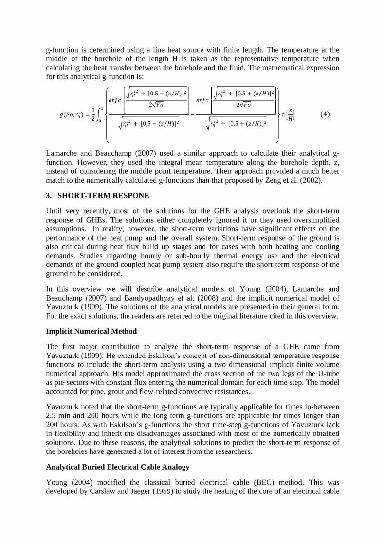
g-function is determined using a line heat source with finite length. The temperature at the

middle of the borehole of the length H is taken as the representative temperature when

calculating the heat transfer between the borehole and the fluid. The mathematical expression

for this analytical g-function is:

𝑔 𝐹𝑜, 𝑟𝐻∗ =

1

2

𝑒𝑟𝑓𝑐

𝑟𝐻

∗2 + 0.5 − (𝑧 𝐻) 2

2 𝐹𝑜

𝑟𝐻∗2 + 0.5 − (𝑧 𝐻) 2

−

𝑒𝑟𝑓𝑐

𝑟𝐻

∗2 + 0.5 + (𝑧 𝐻) 2

2 𝐹𝑜

𝑟𝐻∗2 + 0.5 + (𝑧 𝐻) 2

1

0

d 𝑧

𝐻 (4)

Lamarche and Beauchamp (2007) used a similar approach to calculate their analytical g-

function. However, they used the integral mean temperature along the borehole depth, z,

instead of considering the middle point temperature. Their approach provided a much better

match to the numerically calculated g-functions than that proposed by Zeng et al. (2002).

3. SHORT-TERM RESPONE

Until very recently, most of the solutions for the GHE analysis overlook the short-term

response of GHEs. The solutions either completely ignored it or they used oversimplified

assumptions. In reality, however, the short-term variations have significant effects on the

performance of the heat pump and the overall system. Short-term response of the ground is

also critical during heat flux build up stages and for cases with both heating and cooling

demands. Studies regarding hourly or sub-hourly thermal energy use and the electrical

demands of the ground coupled heat pump system also require the short-term response of the

ground to be considered.

In this overview we will describe analytical models of Young (2004), Lamarche and

Beauchamp (2007) and Bandyopadhyay et al. (2008) and the implicit numerical model of

Yavuzturk (1999). The solutions of the analytical models are presented in their general form.

For the exact solutions, the readers are referred to the original literature cited in this overview.

Implicit Numerical Method

The first major contribution to analyze the short-term response of a GHE came from

Yavuzturk (1999). He extended Eskilson‟s concept of non-dimensional temperature response

functions to include the short-term analysis using a two dimensional implicit finite volume

numerical approach. His model approximated the cross section of the two legs of the U-tube

as pie-sectors with constant flux entering the numerical domain for each time step. The model

accounted for pipe, grout and flow-related convective resistances.

Yavuzturk noted that the short-term g-functions are typically applicable for times in-between

2.5 min and 200 hours while the long term g-functions are applicable for times longer than

200 hours. As with Eskilson‟s g-functions the short time-step g-functions of Yavuzturk lack

in flexibility and inherit the disadvantages associated with most of the numerically obtained

solutions. Due to these reasons, the analytical solutions to predict the short-term response of

the boreholes have generated a lot of interest from the researchers.

Analytical Buried Electrical Cable Analogy

Young (2004) modified the classical buried electrical cable (BEC) method. This was

developed by Carslaw and Jaeger (1959) to study the heating of the core of an electrical cable

by steady current. Young, however, used the analogy between a buried electric cable and a

vertical borehole by considering the core, the insulation and the sheath of the cable to

represent respectively the equivalent diameter fluid pipe, the resistance and the grout of the

GHE. A grout allocation factor (f) allocating a portion of the thermal capacity of the grout to

the core, was also introduced to provide a better fit for ground heat exchanger modelling. The

classical solution to the BEC problem has the following general form as proposed by Carslaw

and Jaeger.

𝑇 − 𝑇0 =𝑞 𝑏𝜆

2𝛼12𝛼2

2

𝜋3

1 − 𝑒−𝑢2𝐹𝑜

𝑢3 ∆(𝑢)

∞

0

𝑑𝑢 (5)

Analytical Solutions for Composite Media

Lamarche and Beauchamp (2007) developed analytical solutions for short-term analysis of

vertical boreholes by considering a hollow cylinder of radius re inside the grout which is

surrounded by infinite homogeneous ground. The cylinder, the grout and the surrounding

ground all represent different media and have different thermal properties. Assuming that the

cylinder reaches a steady flux condition much earlier than the adjacent grout, analytical

solutions for short-term response of the GHE were developed for two cases of constant flux

and of convective heat transfer with known mean fluid temperature. For the first case, with a

known heat per unit length (𝑞 𝑏 ) the proposed solution is:

𝑇 − 𝑇0 =𝑞 𝑏𝜆

8 (𝜆 𝜆𝑔𝑟𝑜𝑢𝑡 )

𝜋5𝑟𝑒∗ 2

(1 − 𝑒−𝑢2𝐹𝑜)

𝑢5 𝜙𝑐2 + 𝜓𝑐

2

∞

0

𝑑𝑢, 𝐹𝑜 =𝑎𝑡

𝑟𝑒2

(6)

For the second case with convective heat transfer and with a known constant fluid

temperature, Tf, the solution takes the following form:

𝑇 = 𝑇𝑓 + 𝑇0 − 𝑇𝑓 16 𝐵𝑖 (𝜆 𝜆𝑔𝑟𝑜𝑢𝑡 )

𝜋4𝑟𝑒∗ 2

𝑒−𝑢2𝐹𝑜

𝑢3 𝜙𝑐2 + 𝜓𝑐

2

∞

0

𝑑𝑢 (7)

Analytical Virtual Solid Model

More recently Bandyopadhyay et al. (2008) have modelled the short-term response of a GHE

in a non-steady-state situation. The model takes the thermal capacity of the circulating fluid

into account by the S/Score ratio which is the ratio of the thermal capacity of an equivalent

volume to the thermal capacity of the core and also considers the flow related convective heat

transfer using Biot number. The circulating fluid in the GHE is modelled as a „virtual solid‟

surrounded by infinite homogeneous medium. The heat transferred to the „virtual solid‟ is

assumed to be generated uniformly over its length. The following classical solution proposed

by Blackwell is applicable under these conditions.

𝑇 − 𝑇0 =𝑞 𝑏

𝜆𝑔𝑟𝑜𝑢𝑡

8

𝜋3

𝑆

Score

2

1 − 𝑒−𝑢2𝐹𝑜

𝑢3 𝑂2 + 𝑃2

∞

0

𝑑𝑢 (8)

DISCUSSION

The short and long term responses of GHE are determined using different approaches. When

determining the long-term response of the GHE the geometry of the borehole is often

neglected and the borehole is modelled either as a line or as a cylindrical source with finite or

infinite lengths. Due to these unrealistic assumptions regarding the geometry of the borehole,

the thermal capacities of the borehole elements and the flow-related convective heat transfer

inside the borehole are also ignored when analyzing the long term response of the GHE.

Bernier (2004) and Nagano (2006) have developed calculation tools using classical CS and

LS methods. However, Eskilson‟s g-function approach, based on the finite LS assumption, is

considered as the state-of-the-art and it has been implemented in many building energy

simulation software including EED, TRANSYS, Energy Plus and GLEHEPRO.

Short-term response of a GHE, on the other hand, requires more stringent assumptions and the

GHE cannot be simply modelled as a line or a cylindrical source. The actual geometry of the

borehole is therefore usually retained when determining its short-term response. An

equivalent diameter is used for simplifications instead of considering a U-tube with two legs.

The equivalent diameter assumption allows taking the thermal mass of the borehole elements

and the flow-related convective resistances into account. The short-term g-functions

developed by Yavuzturk (1999) are regarded as the-state-of-the-art in determining the short-

term response of GHE. Like the g-function approach of Eskilson, the short-term g-function

approach has also been implemented in various building simulation and ground loop design

software including TRANSYS, Energy Plus and GLEHEPRO.

It is appropriate to highlight that the temperature response of a GHE as predicted by almost all

the models is of the following general form.

𝑇 − 𝑇0 =𝑞 𝑏𝜆

𝑓(𝐹𝑜) (9)

This indicates that the load on the GHE and its thermal conductivity are the two significant

factors in addition to the response of the GHE, i.e. f(Fo). As seen in figure 1, the short-term

response of a borehole is independent of size and configuration of its borehole field. The

long-term response, however, is strongly influenced by these factors.

CONCLUSION

The solutions predicted by the analytical models are all functions of the (q b λ) ratio

multiplied to a function of Fourier number. The simple analytical models described in this

paper can be used with reasonable accuracy to predict the response of GHEs with a single

borehole. However, there is a shortage of such models when it comes to multiple borehole

models. There is a genuine need of an analytical model capable of simulating both the short

and the long-term response of the GHE ideally considering all of the significant heat transfer

processes related to the GHE and without distorting the actual geometry of the borehole.

NOMENCLATURE

𝑎 ground thermal diffusivity (𝑚2 𝑠−1) 𝑧 axial coordinate (m)

𝐵𝑖 Biot number = hr λ

𝐹𝑜 Fourier number = at r2 Greek Symbols

𝐻 active borehole depth (m) 𝜆 ground thermal conductivity (W 𝑚−1𝐾−1)

𝐽𝑥 xth − order Basel function of first kind

𝑞 𝑏 heat flow per unit length of GHE (W 𝑚−1) Subscripts

𝑟𝑥∗ non-dimensional radius 𝑏 considering borehole radius 𝑟b

𝑆 unit length thermal capacity (J K-1 m-1 ) 𝑒 considering radius 𝑟e

𝑡 time (s) 𝑓 fluid

𝑇 temperature (K) 𝐻 considering borehole depth

𝑢 integral parameter 𝑠 steady − state

𝑌𝑥 xth − order Basel function of second kind 0 undisturbed

REFERENCES:

Abramovitz, M. and Stegun, I., Eds. (1964). Handbook of Mathematical Functions. National Bureau of

Standards, Washington D.C.

Al-Khoury, R. and Bonnier, P. (2006). Efficient finite element formulation for geothermal heating systems. Part

II: transient. International Journal for Numerical Methods in Engineering 67(5): 725-745.

Al-Khoury, R., Bonnier, P. & Brinkgreve, B. (2005). Efficient finite element formulation for geothermal heating

systems. Part I: steady state. International Journal for Numerical Methods in Engineering 63(7): 988-1013.

Bandyopadhyay, G., Gosnold, W. and Mann, M. (2008). Analytical and semi-analytical solutions for short-time

transient response of ground heat exchangers. Energy and Buildings 40(10): 1816-1824.

Bernier, M. A. (2001). Ground-coupled heat pump system simulation. ASHRAE Transactions 106(1): 605-616.

Bernier, M. A., Labib, R., Pinel, P. and Paillot, R. (2004). A Multiple load aggregation algorithm for annual

hourly simulations of GCHP systems. HVAC&R Research 10(4): 471-487.

Carslaw, H. S. and Jaeger, J. C. (1959). Conduction of heat in solids. Oxford University Press, Oxford.

Eskilson, P. (1987). Thermal analysis of heat extraction boreholes. Doctoral thesis, Lund University, Sweden.

Eskilson, P. and Claesson, J. (1988). Simulation model for thermally interacting heat extraction boreholes.

Numerical Heat Transfer 13: 149-165.

Hart, P. and Couvillion, R. (1986). Earth coupled heat transfer. National Water Well Association, Dublin, OH.

Ingersoll, L. R. and Plass, H. J. (1948). Theory of the ground pipe heat source for the heat pump. Heating, Piping

& Air Conditioning 20(7): 119-122.

Ingersoll, L. R., Zobel, O. J. and Ingersoll, A. C. (1954). Heat conduction with engineering, geological and other

applications. McGraw-Hill, New York.

Kavanaugh, S. P. (1985). Simulation and experimental verification of vertical ground-coupled heat pump

systems. Doctoral thesis, Oklahoma State University, USA.

Kelvin, T. W. (1882). Mathematical and physical papers. Cambridge University Press, London.

Lamarche, L. and Beauchamp, B. (2007). A new contribution to the finite line-source model for geothermal

boreholes. Energy and Buildings 39(2): 188-198.

Lamarche, L. and Beauchamp, B. (2007). New solutions for the short-time analysis of geothermal vertical

boreholes. International Journal of Heat and Mass Transfer 50(7-8): 1408-1419.

Lund, J. W., Freeston, D. H. and Boyd, T. L. (2005). Direct application of geothermal energy: 2005 Worldwide

review. Geothermics 34(6): 691-727.

Muraya, N. K. (1994). Numerical modeling of the transient thermal interference of vertical U-tube heat

exchangers. Doctoral thesis, Texas A&M University, USA.

Nagano, K., Katsura, T. and Takeda, S. (2006). Development of a design and performance prediction tool for the

ground source heat pump system. Applied Thermal Engineering 26(14-15): 1578-1592.

Yavuzturk, C. (1999). Modelling of vertical ground loop heat exchangers for ground source heat pump systems.

Doctoral Thesis, Oklahoma State University, USA.

Young, T. R. (2004). Development, verification, and design analysis of the borehole fluid thermal mass model

for approximating short term borehole thermal response Master's thesis, Oklahoma State University, USA.

Zeng, H. Y., Diao, N. R. and Fang, Z. H. (2002). A finite line-source model for boreholes in geothermal heat

exchangers. Heat Transfer - Asian Research 31(7): 558-567.

Zeng, H. Y., Diao, N. R. and Fang, Z. H. (2003). Heat transfer analysis of boreholes in vertical ground heat

exchangers. International Journal of Heat and Mass Transfer 46(23): 4467-4481.