Embed Size (px)
Citation preview
EFFICIENT USE OF HYBRID ADAPTIVE NEURO-FUZZY
INFERENCE SYSTEM COMBINED WITH NONLINEAR
DIMENSION REDUCTION METHOD IN PRODUCTION
PROCESSES
Saad Bashir Alvi,
Robert Martin,
Johannes Gottschling
Mathematics for Engineer, Duisburg-Essen University, Duisburg
[email protected] [email protected]
ABSTRACT
This research study proposes a novel method for automatic fault prediction from foundry data introducing the so-
called Meta Prediction Function (MPF). Kernel Principal Component Analysis (KPCA) is used for dimension
reduction. Different algorithms are used for building the MPF such as Multiple Linear Regression (MLR), Adaptive
Neuro Fuzzy Inference System (ANFIS), Support Vector Machine (SVM) and Neural Network (NN). We used classical
machine learning methods such as ANFIS, SVM and NN for comparison with our proposed MPF. Our empirical results
show that the MPF consistently outperform the classical methods.
KEYWORDS
Fuzzy Inference System, ANFIS, Neural Network, Support Vector Machine, KPCA
1. INTRODUCTION
Automatic fault prediction is an important topic of research in metal industry [1]. Since the beginning of the
first industrial revolution, industries are striving to produce fault-free products in least possible amount of
time. Customer expectations are ever-increasing in term of quality and availability of products [2-4]. A fault
in a product during the production process can be due to a single cause or a combination of causes and
industries are still using trial and error methods to minimize them [5][6]. Faults in production can be reduced
by analysis of the production process data [7][8]. Data capturing of the production processes for analysis
started manually but due to human-errors, the quality of the data captured was compromised. Now, with the
automation of data capturing using sensors, the noisy data is getting reduced. With the advancement of the
technology and automation, more and more data is available for analysis to optimise the production
processes [9].
In the current globalized industry era with emphasis on automated smart industries, the analysis of measured
data plays an important role to improve the quality of the products [10]. Large number of parameters have
an influence on the quality of a product. Deviations of process parameters can have negative effect on the
production performance. Measuring and evaluating all the appropriate process parameters with a suitable
method ensure a consistently high quality and productivity in the automated production environment. The
application of Machine Learning (ML) methods in these processes is motivated mainly by two objectives:
the prediction of quality properties from the measured data and the identification of key process indicators,
i.e. the process parameters which have the strongest influence on the outcome. These objectives help to
improve the quality of the products and to understand the implicit relations among the parameters in the
production processes, which in turn result in reducing faulty products during production.
In this work, we will concentrate on the first objective, namely the prediction of quality properties from the
measured data by suggesting a novel methodology for automatic fault prediction. The learnt methodology
will help to reach target predictions, which will ensure stability of the production process regulation and
repeatability of the process conditions resulting in quality products with minimal scrap. The potential of the
proposed methodology is demonstrated by using three actual production datasets.
In our approach, we use three stage process. In first stage, the input data is split into mutually exclusive sets
of training, validation and test data. In the second stage, Support Vector Machine (SVM) [11][12] and
Neural Network (NN) [13][14] are trained using the original data whereas Adaptive Neuro Fuzzy Inference
System (ANFIS) [15] is trained on the data transformed by Kernel Principal Component Analysis (KPCA)
[16][17]. In the last stage, we utilize a novel fusion method to combine these different prediction functions
and obtain a “Meta Prediction Function" (MPF). Results during these stages are also collected and
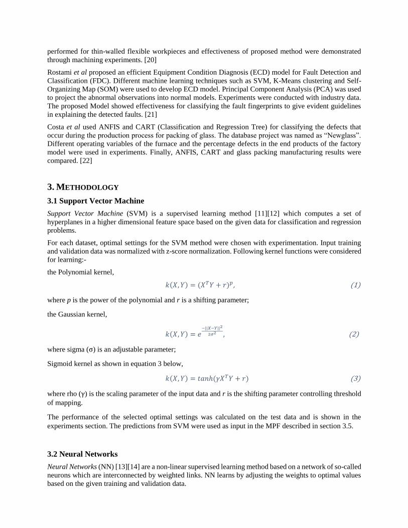
performance is measured. Figure 1 shows major data processing units of proposed framework.
Figure 1 - Major data processing blocks
The performance of the MPF is compared with the performance of the classical machine learning methods
such as Neural Networks, SVM and ANFIS.
2. RELATED WORK
Leha et al proposed a novel integrated method into a production plan realized in a physics-based realistic
simulator. Supervised machine learning techniques namely Model Trees and Neural Networks were
integrated. The online learning and on the fly control code modification were allowed by integrating the
learning capability into the control process. Averaging was used for measuring the produced optimization
times through learning which outperform times of a production process. [18]
Ashour et al proposed a method for automated identification for machined surfaces in manufacturing. Image
processing and computer vision technologies were used for automated identification for reduction in
inspection time and avoidance of human error due to inconsistency and fatigue. SVM classifier with
different kernels were investigated for the categorization of machined surfaces into six machining processes.
The gray level histogram was used as discriminating feature. Experimental results suggested that the SVM
with the linear kernel outperformed for a dataset consisting of seventy-two workpiece images. [19]
Yuan et al proposed a novel method for improving the machining quality of thin walled flexible workpieces.
Machining platform was established for thin-walled flexible workpieces. Sparse Bayesian learning based
method was used to predict the future deformation. The dual mode predictive controller was developed to
reduce the machining vibrations and quality of the workpiece surface was improved. Experiments were
5. Meta-Prediction Function
2. KPCA and ANFIS
learning
3. Support Vector
Machines (SVM)
learning
4. Neural Networks
(NN) learning
1. Data Splitting
performed for thin-walled flexible workpieces and effectiveness of proposed method were demonstrated
through machining experiments. [20]
Rostami et al proposed an efficient Equipment Condition Diagnosis (ECD) model for Fault Detection and
Classification (FDC). Different machine learning techniques such as SVM, K-Means clustering and Self-
Organizing Map (SOM) were used to develop ECD model. Principal Component Analysis (PCA) was used
to project the abnormal observations into normal models. Experiments were conducted with industry data.
The proposed Model showed effectiveness for classifying the fault fingerprints to give evident guidelines
in explaining the detected faults. [21]
Costa et al used ANFIS and CART (Classification and Regression Tree) for classifying the defects that
occur during the production process for packing of glass. The database project was named as “Newglass”.
Different operating variables of the furnace and the percentage defects in the end products of the factory
model were used in experiments. Finally, ANFIS, CART and glass packing manufacturing results were
compared. [22]
3. METHODOLOGY
3.1 Support Vector Machine
Support Vector Machine (SVM) is a supervised learning method [11][12] which computes a set of
hyperplanes in a higher dimensional feature space based on the given data for classification and regression
problems.
For each dataset, optimal settings for the SVM method were chosen with experimentation. Input training
and validation data was normalized with z-score normalization. Following kernel functions were considered
for learning:-
the Polynomial kernel,
𝑘(𝑋, 𝑌) = (𝑋𝑇𝑌 + 𝑟)𝑝, (1)
where p is the power of the polynomial and r is a shifting parameter;
the Gaussian kernel,
𝑘(𝑋, 𝑌) = 𝑒−||𝑋−𝑌||2
2𝜎2 , (2)
where sigma (σ) is an adjustable parameter;
Sigmoid kernel as shown in equation 3 below,
𝑘(𝑋, 𝑌) = 𝑡𝑎𝑛ℎ(𝛾𝑋𝑇𝑌 + 𝑟) (3)
where rho (γ) is the scaling parameter of the input data and r is the shifting parameter controlling threshold
of mapping.
The performance of the selected optimal settings was calculated on the test data and is shown in the
experiments section. The predictions from SVM were used as input in the MPF described in section 3.5.
3.2 Neural Networks
Neural Networks (NN) [13][14] are a non-linear supervised learning method based on a network of so-called
neurons which are interconnected by weighted links. NN learns by adjusting the weights to optimal values
based on the given training and validation data.
In this work, a NN is trained using one of the most popular backpropagation learning algorithm with
multilayer perceptron topology. The used feedforward NN consisted of three layers: an input layer, one
hidden layer and an output layer. The number of neurons in the input layer is equal to the total number of
independent variables and the number of neurons in the output layer is equal to the number of dependent
variables, whereas the hidden layer contains eight neurons for all considered datasets. The input layer
receives the input from the independent variables and forwards it to all the neurons in the hidden layer. The
neurons in the hidden layer apply their activation function to the weighted sum of their inputs and compute
an output. The output layer then computes the predicted value for the dependent variable(s).
The back-propagation learning algorithm used here to train the multilayer network consists of two passes.
In the forward pass, with randomly selected weights and the input given by the training data, the algorithm
produces an output for the dependent variable(s). An error is then calculated based on the difference between
predicted and actual output. In the backward pass, this error is propagated backwards through the network
from the output layer to the input layer and weights in the network are modified using the delta rule. The
formula used to calculate the change in weights of hidden and output layer neurons are shown in equation
4 and in equation 5 respectively:-
∆𝑤𝑖𝑗(𝑝) = 𝛽. ∆𝑤𝑖𝑗(𝑝 − 1) + 𝛼. 𝑥𝑖(𝑝). 𝛿𝑗(𝑝) (4) ∆𝑤𝑗𝑘(𝑝) = 𝛽. ∆𝑤𝑗𝑘(𝑝 − 1) + 𝛼. 𝑦𝑗(𝑝). 𝛿𝑘(𝑝) (5)
where the indices i, j, k refer to input, hidden and output layers,
𝛼 is the learning rate,
𝛽 is the Momentum with a value between 0 and 1,
𝑥𝑖(𝑝), 𝑦𝑗(𝑝) are the output of neurons i in the input layer and j in the hidden layer at iteration p,
𝛿𝑗(𝑝), 𝛿𝑘(𝑝) are the error gradients at the neurons j in hidden layer and k in the output layer at iteration p.
During training, we used 1000 epochs. Weights of the NN were optimised using settings of learning rate
0.1 and momentum 0.2. The Unipolar Sigmoid function was used as the activation function.
During the learning phase, training and validation data is normalised. Then NN is trained and the
parameter settings which produce best results are preserved and the performance of these settings is
calculated on the test data.
The predictions from NN are also used as input in the MPF in section 3.5.
3.3 Kernel Principal Component Analysis
Kernel Principal Component Analysis (KPCA) is a nonlinear dimension reduction method, introduced by
Sholkopt et al. [16][17], which maps data from the input space to a lower dimensional feature space while
retaining maximum possible variance in the data.
For each dataset, KPCA was applied using the Polynomial kernel and Gaussian kernel, which are defined
in equations (1) and (2) respectively. For the Polynomial kernel, settings used were p = 1,2,3; r = 0. For
Gaussian kernel, the settings used were σ = 0.5, 1.0, 1.5.
The results are shown for the kernel settings which provided the most accurate prediction results.
3.4 Adaptive Neuro-Fuzzy Inference System
Adaptive Neuro-Fuzzy Inference System (ANFIS) [15] is a hybrid neuro-fuzzy model which consists of 5
layers. In the first layer, for the inputs, degree of membership of the chosen membership function is
computed. In the second layer, firing strength of the rules is calculated using t-norm (product for AND and
maximum for OR) operators. In the third layer, computed firing strengths are normalized. Forth layer is the
adaptation layer in which rule consequent parameters are computed. Fifth layer is the summation layer
which computes sum of all the computed consequents. In learning phase of ANFIS, membership function
parameters and rules consequent parameters are optimised.
In our approach, we use the ANFIS, which combines the advantages of fuzzy expert systems with those of
classical NN, in combination with KPCA. It has already been successfully employed for data prediction in
a variety of fields. KPCA was used to transform the data because for some of the selected parameter settings
like input partition method: ‘grid partitioning’, ANFIS was not immediately applicable to the number of
variables as large as 10. In addition, even in the case of small number of variables, it was observed that
ANFIS produced comparatively better results for same parameter settings on the transformed data from
KPCA in comparison to the original data as input.
Before the training in ANFIS start, a Fuzzy Inference System (FIS) is initialized with information about the
number of input variables for the selected dataset, the selected number and type of membership functions
and the number of rules. The rules for the FIS were initialized based on the Grid Partitioning (GP) method
or Subtractive Clustering (SC) method. In case of GP method, input membership function type as Gaussian
was selected, output membership function type as Linear was selected and in different independent runs for
best parameter settings, number of membership functions for input parameters were selected as 2, 3 or 4.
For SC method, influence radius was tested with inputs 0.1, 0.2, 0.3, 0.4 and 0.5 for different runs. It was
trained using NN backpropagation algorithm and least square methods.
In case of KPCA and ANFIS, the training and validation data was collectively normalised and the
corresponding symmetric kernel matrix was computed. The Eigen-values and Eigen-vectors were computed
for the computed kernel matrix. Then principal components of the training and validation data were
computed using the computed kernel matrix and Eigen-vectors. These principal components along with the
corresponding dependent variable values were used to train ANFIS and parameter settings which produced
the best result on the validation data were saved. Finally, the performance was calculated on the principal
components of the test data. These predictions were also saved for later use in the MPF.
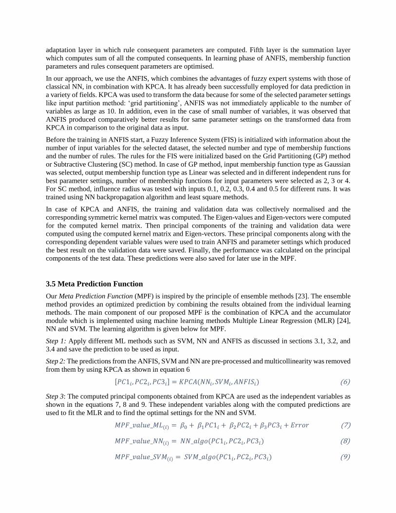
3.5 Meta Prediction Function
Our Meta Prediction Function (MPF) is inspired by the principle of ensemble methods [23]. The ensemble
method provides an optimized prediction by combining the results obtained from the individual learning
methods. The main component of our proposed MPF is the combination of KPCA and the accumulator
module which is implemented using machine learning methods Multiple Linear Regression (MLR) [24],
NN and SVM. The learning algorithm is given below for MPF.
Step 1: Apply different ML methods such as SVM, NN and ANFIS as discussed in sections 3.1, 3.2, and
3.4 and save the prediction to be used as input.
Step 2: The predictions from the ANFIS, SVM and NN are pre-processed and multicollinearity was removed
from them by using KPCA as shown in equation 6
[𝑃𝐶1𝑖, 𝑃𝐶2𝑖, 𝑃𝐶3𝑖] = 𝐾𝑃𝐶𝐴(𝑁𝑁𝑖 , 𝑆𝑉𝑀𝑖, 𝐴𝑁𝐹𝐼𝑆𝑖) (6)
Step 3: The computed principal components obtained from KPCA are used as the independent variables as
shown in the equations 7, 8 and 9. These independent variables along with the computed predictions are
used to fit the MLR and to find the optimal settings for the NN and SVM.
𝑀𝑃𝐹_𝑣𝑎𝑙𝑢𝑒_𝑀𝐿(𝑖) =𝛽0 +𝛽1𝑃𝐶1𝑖 +𝛽2𝑃𝐶2𝑖 + 𝛽3𝑃𝐶3𝑖 + 𝐸𝑟𝑟𝑜𝑟 (7)
𝑀𝑃𝐹_𝑣𝑎𝑙𝑢𝑒_𝑁𝑁(𝑖) = 𝑁𝑁_𝑎𝑙𝑔𝑜(𝑃𝐶1𝑖, 𝑃𝐶2𝑖, 𝑃𝐶3𝑖) (8)
𝑀𝑃𝐹_𝑣𝑎𝑙𝑢𝑒_𝑆𝑉𝑀(𝑖) = 𝑆𝑉𝑀_𝑎𝑙𝑔𝑜(𝑃𝐶1𝑖, 𝑃𝐶2𝑖, 𝑃𝐶3𝑖) (9)
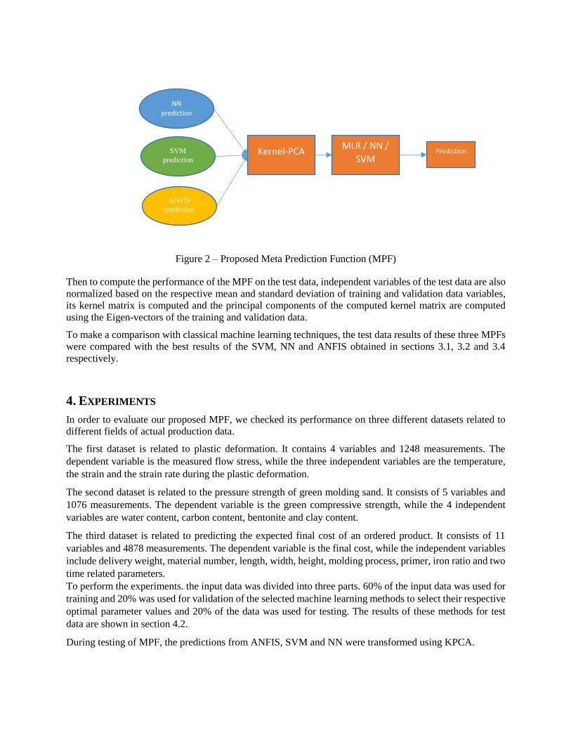
Figure 2 – Proposed Meta Prediction Function (MPF)
Then to compute the performance of the MPF on the test data, independent variables of the test data are also
normalized based on the respective mean and standard deviation of training and validation data variables,
its kernel matrix is computed and the principal components of the computed kernel matrix are computed
using the Eigen-vectors of the training and validation data.
To make a comparison with classical machine learning techniques, the test data results of these three MPFs
were compared with the best results of the SVM, NN and ANFIS obtained in sections 3.1, 3.2 and 3.4
respectively.
4. EXPERIMENTS
In order to evaluate our proposed MPF, we checked its performance on three different datasets related to
different fields of actual production data.
The first dataset is related to plastic deformation. It contains 4 variables and 1248 measurements. The
dependent variable is the measured flow stress, while the three independent variables are the temperature,
the strain and the strain rate during the plastic deformation.
The second dataset is related to the pressure strength of green molding sand. It consists of 5 variables and
1076 measurements. The dependent variable is the green compressive strength, while the 4 independent
variables are water content, carbon content, bentonite and clay content.
The third dataset is related to predicting the expected final cost of an ordered product. It consists of 11
variables and 4878 measurements. The dependent variable is the final cost, while the independent variables
include delivery weight, material number, length, width, height, molding process, primer, iron ratio and two
time related parameters.
To perform the experiments. the input data was divided into three parts. 60% of the input data was used for
training and 20% was used for validation of the selected machine learning methods to select their respective
optimal parameter values and 20% of the data was used for testing. The results of these methods for test
data are shown in section 4.2.
During testing of MPF, the predictions from ANFIS, SVM and NN were transformed using KPCA.
NN
prediction
Kernel-PCA MLR / NN /
SVM Prediction SVM
prediction
ANFIS
prediction
4.1 Performance evaluation measure
To check the performance of the selected machine learning methods, three different error measures were
computed namely Root Mean Square Error (RMSE), Relative Root Mean Square Error (RRMSE) and
Symmetric Mean Absolute Percentage Error (SMAPE), which are defined as
𝑅𝑀𝑆𝐸 =√1
𝑛∑ |𝑂𝑖 − 𝑃𝑖|
2𝑛𝑖=1 (10)
𝑅𝑅𝑀𝑆𝐸 =√1
𝑛∑
|𝑂𝑖−𝑃𝑖|2
|𝑂𝑖|2
𝑛𝑖=1 (11)
𝑆𝑀𝐴𝑃𝐸 =1
𝑛∑
|𝑂𝑖−𝑃𝑖|
(|𝑂𝑖|+|𝑃𝑖|)/2𝑛𝑖=1 (12)
where n is the total number of patterns. 𝑂𝑖is the computed output and 𝑃𝑖is the predicted output from the
used machine learning method.
4.2 Results and Discussion
4.2.1 Results for dataset Flow Stress
First dataset we used to observe our method performance contains actual measurements from metal forming
experiments.
For NN, same settings were used as described in the section 3.2 For SVM, Gaussian kernel with sigma (𝜎)
value of 0.5 produced best results.
Since the number of independent variables is smaller in this instance, after computing the principal
components, all three of them were selected, covering 100% of the variance in the data. For ANFIS, Linear
kernel along with subtractive clustering (radius: 0.2) produced best results as shown in the Table 1 below.
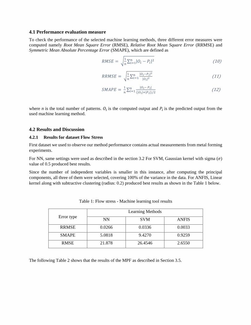
Table 1: Flow stress - Machine learning tool results
Error type
Learning Methods
NN SVM ANFIS
RRMSE 0.0266 0.0336 0.0033
SMAPE 5.0818 9.4270 0.9259
RMSE 21.878 26.4546 2.6550
The following Table 2 shows that the results of the MPF as described in Section 3.5.
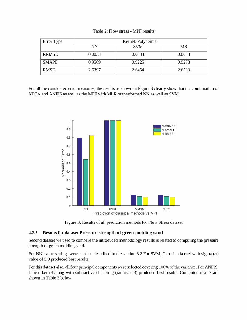
Table 2: Flow stress - MPF results
Error Type Kernel: Polynomial
NN SVM MR
RRMSE 0.0033 0.0033 0.0033
SMAPE 0.9569 0.9225 0.9278
RMSE 2.6397 2.6454 2.6533
For all the considered error measures, the results as shown in Figure 3 clearly show that the combination of
KPCA and ANFIS as well as the MPF with MLR outperformed NN as well as SVM.
Figure 3: Results of all prediction methods for Flow Stress dataset
4.2.2 Results for dataset Pressure strength of green molding sand
Second dataset we used to compare the introduced methodology results is related to computing the pressure
strength of green molding sand.
For NN, same settings were used as described in the section 3.2 For SVM, Gaussian kernel with sigma (𝜎)
value of 5.0 produced best results.
For this dataset also, all four principal components were selected covering 100% of the variance. For ANFIS,
Linear kernel along with subtractive clustering (radius: 0.3) produced best results. Computed results are
shown in Table 3 below.
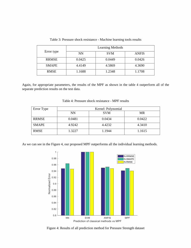
Table 3: Pressure shock resistance - Machine learning tools results
Error type
Learning Methods
NN SVM ANFIS
RRMSE 0.0425 0.0449 0.0426
SMAPE 4.4149 4.5869 4.3690
RMSE 1.1688 1.2348 1.1708
Again, for appropriate parameters, the results of the MPF as shown in the table 4 outperform all of the
separate prediction results on the test data.
Table 4: Pressure shock resistance - MPF results
Error Type Kernel: Polynomial
NN SVM MR
RRMSE 0.0481 0.0434 0.0422
SMAPE 4.9242 4.4232 4.3410
RMSE 1.3227 1.1944 1.1615
As we can see in the Figure 4, our proposed MPF outperforms all the individual learning methods.
Figure 4: Results of all prediction method for Pressure Strength dataset
4.2.3 Results for dataset Final cost
Final cost dataset contains data recorded from actual production environment and is used to predict the
expected final costs of the new ordered product.
For NN, same settings were used as described in the section 3.2 For SVM, Gaussian kernel with sigma (𝜎)
value of 5.0 produced best results.
In this case, seven out of ten principal components were selected covering 95.91% of the variance in the
original data. For ANFIS, Linear kernel along with subtractive clustering (radius: 0.2) produced best results.
Results are shown in Table 5 below.
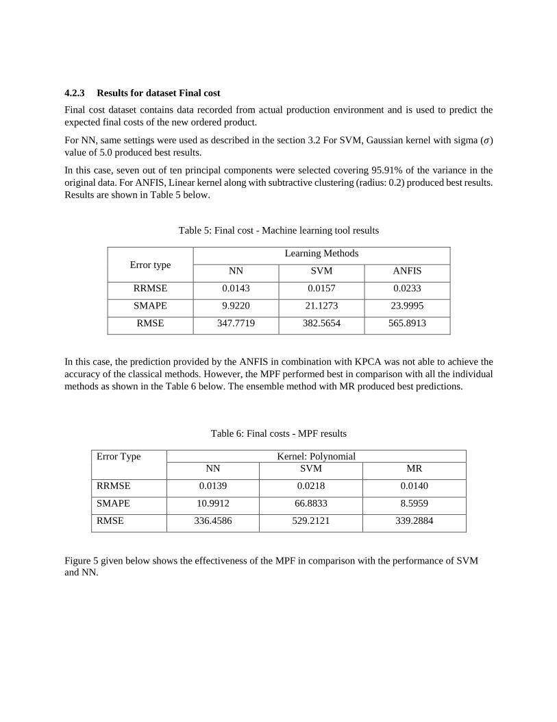
Table 5: Final cost - Machine learning tool results
Error type
Learning Methods
NN SVM ANFIS
RRMSE 0.0143 0.0157 0.0233
SMAPE 9.9220 21.1273 23.9995
RMSE 347.7719 382.5654 565.8913
In this case, the prediction provided by the ANFIS in combination with KPCA was not able to achieve the
accuracy of the classical methods. However, the MPF performed best in comparison with all the individual
methods as shown in the Table 6 below. The ensemble method with MR produced best predictions.
Table 6: Final costs - MPF results
Error Type Kernel: Polynomial
NN SVM MR
RRMSE 0.0139 0.0218 0.0140
SMAPE 10.9912 66.8833 8.5959
RMSE 336.4586 529.2121 339.2884
Figure 5 given below shows the effectiveness of the MPF in comparison with the performance of SVM
and NN.
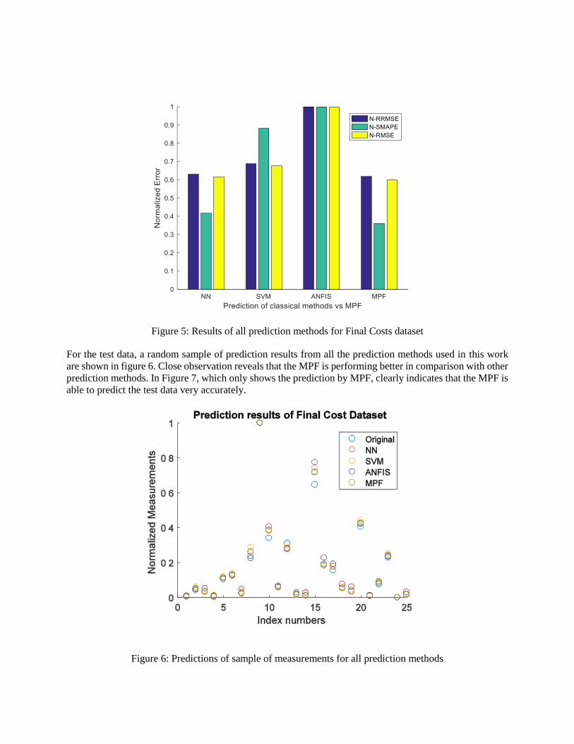
Figure 5: Results of all prediction methods for Final Costs dataset
For the test data, a random sample of prediction results from all the prediction methods used in this work
are shown in figure 6. Close observation reveals that the MPF is performing better in comparison with other
prediction methods. In Figure 7, which only shows the prediction by MPF, clearly indicates that the MPF is
able to predict the test data very accurately.
Figure 6: Predictions of sample of measurements for all prediction methods
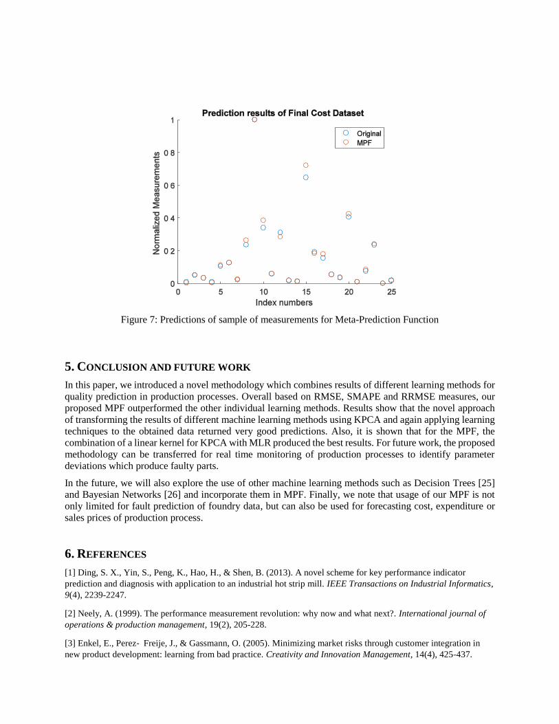
Figure 7: Predictions of sample of measurements for Meta-Prediction Function
5. CONCLUSION AND FUTURE WORK
In this paper, we introduced a novel methodology which combines results of different learning methods for
quality prediction in production processes. Overall based on RMSE, SMAPE and RRMSE measures, our
proposed MPF outperformed the other individual learning methods. Results show that the novel approach
of transforming the results of different machine learning methods using KPCA and again applying learning
techniques to the obtained data returned very good predictions. Also, it is shown that for the MPF, the
combination of a linear kernel for KPCA with MLR produced the best results. For future work, the proposed
methodology can be transferred for real time monitoring of production processes to identify parameter
deviations which produce faulty parts.
In the future, we will also explore the use of other machine learning methods such as Decision Trees [25]
and Bayesian Networks [26] and incorporate them in MPF. Finally, we note that usage of our MPF is not
only limited for fault prediction of foundry data, but can also be used for forecasting cost, expenditure or
sales prices of production process.
6. REFERENCES
[1] Ding, S. X., Yin, S., Peng, K., Hao, H., & Shen, B. (2013). A novel scheme for key performance indicator
prediction and diagnosis with application to an industrial hot strip mill. IEEE Transactions on Industrial Informatics,
9(4), 2239-2247.
[2] Neely, A. (1999). The performance measurement revolution: why now and what next?. International journal of
operations & production management, 19(2), 205-228.
[3] Enkel, E., Perez‐ Freije, J., & Gassmann, O. (2005). Minimizing market risks through customer integration in
new product development: learning from bad practice. Creativity and Innovation Management, 14(4), 425-437.
[4] Kan, S. H., Basili, V. R., & Shapiro, L. N. (1994). Software quality: an overview from the perspective of total
quality management. IBM Systems Journal, 33(1), 4-19.
[5] Sosna, Marc, Rosa Nelly Trevinyo-Rodríguez, and S. Ramakrishna Velamuri. "Business model innovation
through trial-and-error learning: The Naturhouse case." Long range planning 43.2 (2010): 383-407.
[6] Shingo, S., & Dillon, A. P. (1989). A study of the Toyota production system: From an Industrial Engineering
Viewpoint. CRC Press.
[7] Dilts, D. M., Boyd, N. P., & Whorms, H. H. (1991). The evolution of control architectures for automated
manufacturing systems. Journal of manufacturing systems, 10(1), 79-93.
[8] Kang, S., Kim, E., Shim, J., Cho, S., Chang, W., & Kim, J. (2017). Mining the relationship between production
and customer service data for failure analysis of industrial products. Computers & Industrial Engineering, 106, 137-
146.
[9] Fayyad, U., Piatetsky-Shapiro, G., & Smyth, P. (1996). The KDD process for extracting useful knowledge from
volumes of data. Communications of the ACM, 39(11), 27-34.
[10] Ribeiro, L., & Barata, J. (2011). Re-thinking diagnosis for future automation systems: An analysis of current
diagnostic practices and their applicability in emerging IT based production paradigms. Computers in Industry,
62(7), 639-659.
[11] Schölkopf, Bernhard; and Smola, Alexander J.;” Learning with Kernels”, MIT Press, Cambridge, MA, 2002,
ISBN 0-262-19475-9.
[12] Suykens, J. A., & Vandewalle, J. (1999). Least squares support vector machine classifiers. Neural processing
letters, 9(3), 293-300.
[13] Lawrence, Jeanette, “Introduction to Neural Networks”, California Scientific Software Press 1994, ISBN 1-
883157-00-5.
[14] Craven, M. W., & Shavlik, J. W. (1997). Using neural networks for data mining. Future generation computer
systems, 13(2-3), 211-229.
[15] Jang, J-SR. "ANFIS: Adaptive-Network-based Fuzzy Inference System." IEEE transactions on systems, man,
and cybernetics 23.3 (1993): 665-685.
[16] B. Scholkopf, A. Smola, and K. Muller. “Nonlinear component analysis as a kernel eigenvalue problem”. Neural
Computation, 10(5):1299–1319, 1998.
[17] Yang, J., Frangi, A. F., Yang, J. Y., Zhang, D., & Jin, Z. (2005). KPCA plus LDA: a complete kernel Fisher
discriminant framework for feature extraction and recognition. IEEE Transactions on pattern analysis and machine
intelligence, 27(2), 230-244.
[18] Leha, A., Pangercic, D., Rühr, T., & Beetz, M. (2009, September). “Optimization of simulated production process
performance using machine learning”. In Emerging Technologies & Factory Automation, 2009. ETFA 2009. IEEE
Conference on (pp. 1-5). IEEE.
[19] Ashour, M. W., Khalid, F., Halin, A. A., & Abdullah, L. N. (2015, October). “Machining process classification
using PCA reduced histogram features and the Support Vector Machine”. In Signal and Image Processing Applications
(ICSIPA), 2015 IEEE International Conference on (pp. 414-418). IEEE.
[20] Yuan, Y., Zhang, H. T., Wu, Y., Zhu, T., & Ding, H. (2016). Bayesian learning-based model predictive vibration
control for thin-walled workpiece machining processes. IEEE/ASME Transactions on Mechatronics.
[21] Rostami, H., Blue, J., & Yugma, C. (2016, December). Equipment Condition Diagnosis and Fault Fingerprint
Extraction in Semiconductor Manufacturing. In Machine Learning and Applications (ICMLA), 2016 15th IEEE
International Conference on (pp. 534-539). IEEE.

[22] H.R. d. N. Costa and A. La Neve, "A study on the application of regression trees and adaptive neuro-fuzzy
inference system in glass manufacturing process for packaging," 2016 Annual Conference of the North American Fuzzy
Information Processing Society (NAFIPS), El Paso, TX, USA, 2016, pp. 1-4.
[23] Dietterich, Thomas G. "Ensemble methods in machine learning." International workshop on multiple classifier
systems. Springer Berlin Heidelberg, 2000.
[24] Aiken, L. S., West, S. G., & Pitts, S. C. (2003). Multiple linear regression. Handbook of psychology.
[25] Safavian, S. R., & Landgrebe, D. (1991). A survey of decision tree classifier methodology. IEEE transactions
on systems, man, and cybernetics, 21(3), 660-674.
[26] Jansen, R., Yu, H., Greenbaum, D., Kluger, Y., Krogan, N. J., Chung, S., ... & Gerstein, M. (2003). A Bayesian
networks approach for predicting protein-protein interactions from genomic data. science, 302(5644), 449-453.
Saad Bashir Alvi is currently a Ph.D. student and a research associate in the Institute for Technologies of Metals
at the University of Duisburg-Essen. He has previously worked as a software engineer and received his M.Sc.
from University of Bonn, Germany in 2013. His research interests include machine learning and Neural
Networks with special emphasis on comparative studies in predictive analytics and focus on dimension
reduction as well as neuro fuzzy modeling with applications to production processes.
Robert Martin received his Ph.D. from the University of Duisburg-Essen University, Germany in 2016 and is
currently working at the Institute for Technologies of Metals in Duisburg.
Prof. Johannes Gottschling is working at the Institute for Technologies of Metals at the University of Duisburg-
Essen and is head of the chair “Mathematics for Engineers”.