Embed Size (px)
Citation preview

Efficient Storage and Processing of Adaptive Triangular Grids using
Sierpinski Curves
Csaba Attila VighDepartment of Informatics, TU München
JASS 2006, course 2:Numerical Simulation: From Models to Visualizations
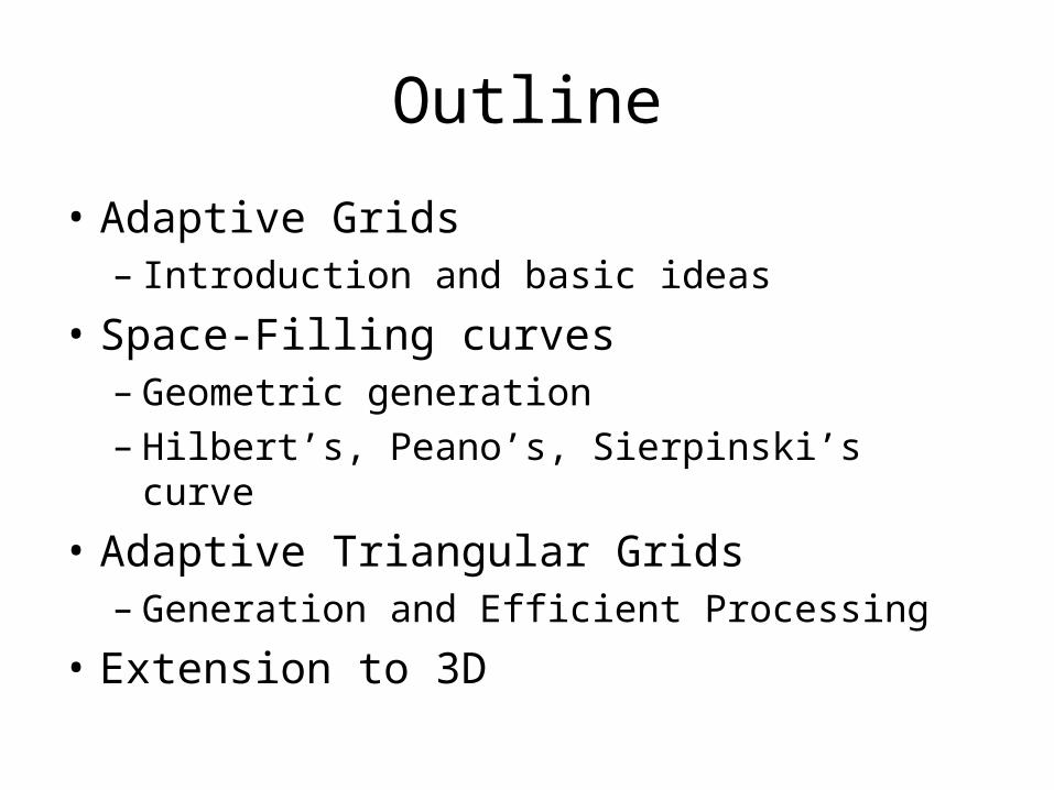
Outline
• Adaptive Grids – Introduction and basic ideas
• Space-Filling curves– Geometric generation– Hilbert’s, Peano’s, Sierpinski’s curve
• Adaptive Triangular Grids– Generation and Efficient Processing
• Extension to 3D
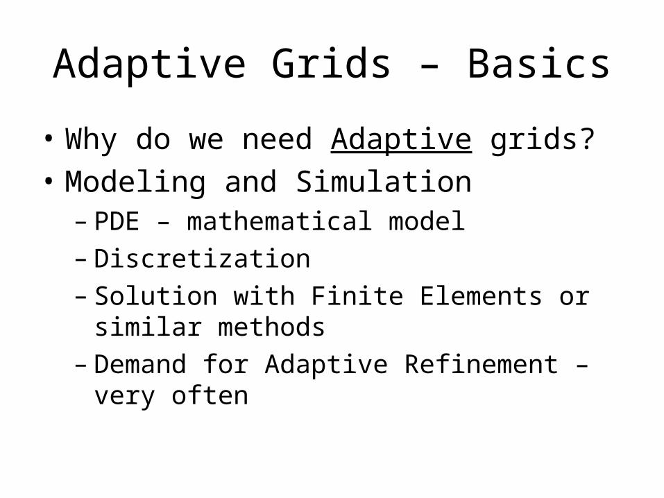
Adaptive Grids – Basics
• Why do we need Adaptive grids?
• Modeling and Simulation– PDE – mathematical model– Discretization – Solution with Finite Elements or similar
methods– Demand for Adaptive Refinement – very often
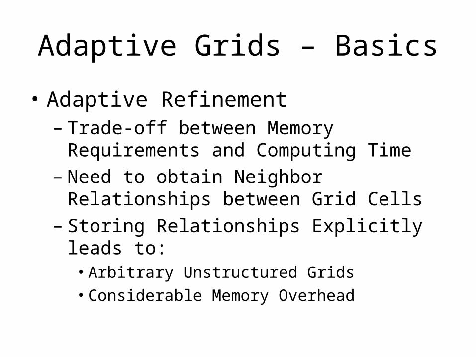
Adaptive Grids – Basics
• Adaptive Refinement– Trade-off between Memory Requirements and
Computing Time– Need to obtain Neighbor Relationships
between Grid Cells– Storing Relationships Explicitly leads to:
• Arbitrary Unstructured Grids• Considerable Memory Overhead
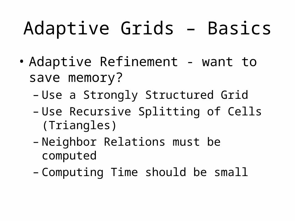
Adaptive Grids – Basics
• Adaptive Refinement - want to save memory?– Use a Strongly Structured Grid– Use Recursive Splitting of Cells (Triangles)– Neighbor Relations must be computed– Computing Time should be small
Adaptive Grids – Basics
• Processing of Recursively Refined (Triangular) Grid– Linearize Access to the Cells using Space-
Filling Curves• For Triangles – Sierpinski Curve
– Use a Stack System for Cache-Efficiency– Parallelization Strategies using Space-Filling
Curves are readily available
Space-Filling Curves
• 1878, Cantor– Any two Finite-Dimensional Manifolds have
same Cardinality– [0, 1] can be Mapped Bijectively onto the
Square [0,1]x[0,1], or onto the Cube
• 1879, Netto – such a Mapping is necessarily Discontinuous

Space-Filling Curves
• Is then possible to obtain a Surjective Continuous Mapping?
or
• Is there a Curve that passes through every Point of a Two-Dimensional Region?
• 1890, Peano constructed the first one
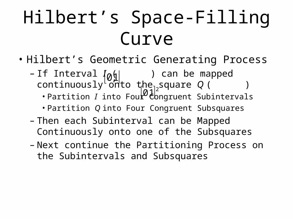
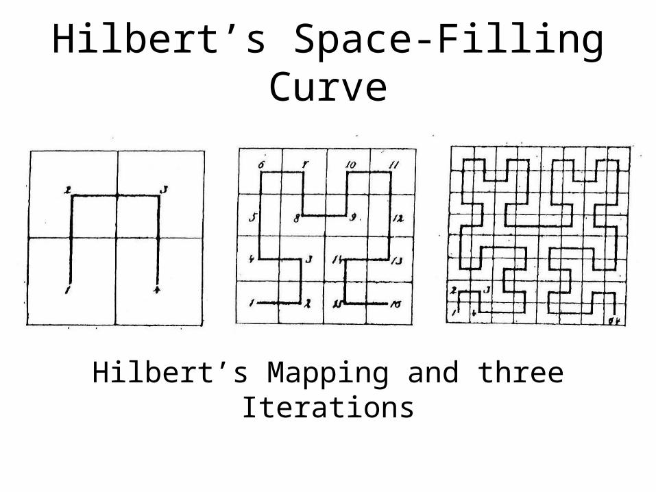
Hilbert’s Space-Filling Curve
• Hilbert’s Geometric Generating Process– If Interval I ( ) can be mapped continuously
onto the square Q ( )• Partition I into Four Congruent Subintervals• Partition Q into Four Congruent Subsquares
– Then each Subinterval can be Mapped Continuously onto one of the Subsquares
– Next continue the Partitioning Process on the Subintervals and Subsquares
1,0 21,0
Hilbert’s Space-Filling Curve
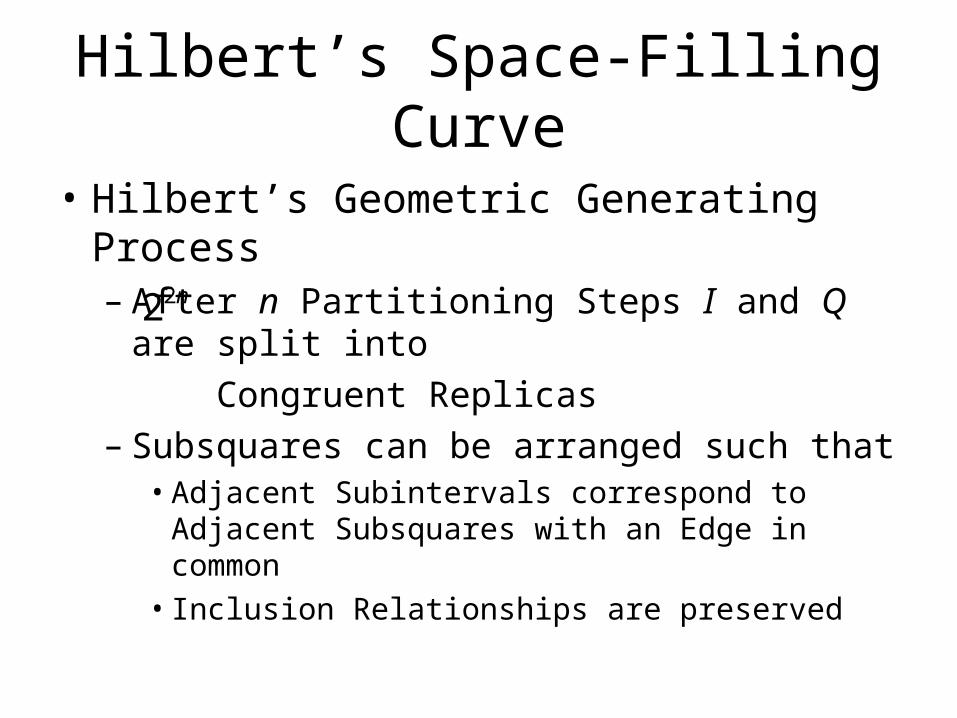
• Hilbert’s Geometric Generating Process– After n Partitioning Steps I and Q are split into
Congruent Replicas– Subsquares can be arranged such that
• Adjacent Subintervals correspond to Adjacent Subsquares with an Edge in common
• Inclusion Relationships are preserved
n22
Hilbert’s Space-Filling Curve
Hilbert’s Mapping and three Iterations
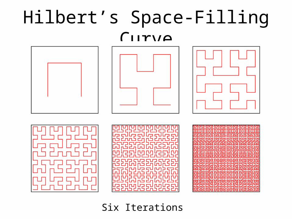
Hilbert’s Space-Filling Curve
Six Iterations
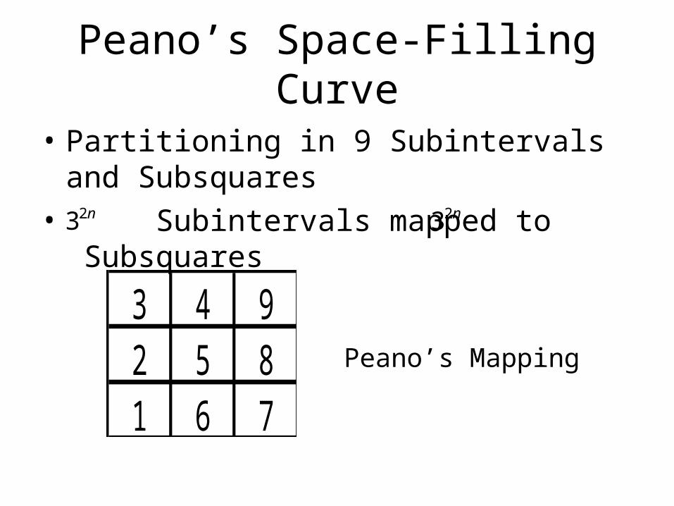
Peano’s Space-Filling Curve
• Partitioning in 9 Subintervals and Subsquares
• Subintervals mapped to Subsquaresn23 n23
3 4 92 5 81 6 7
Peano’s Mapping
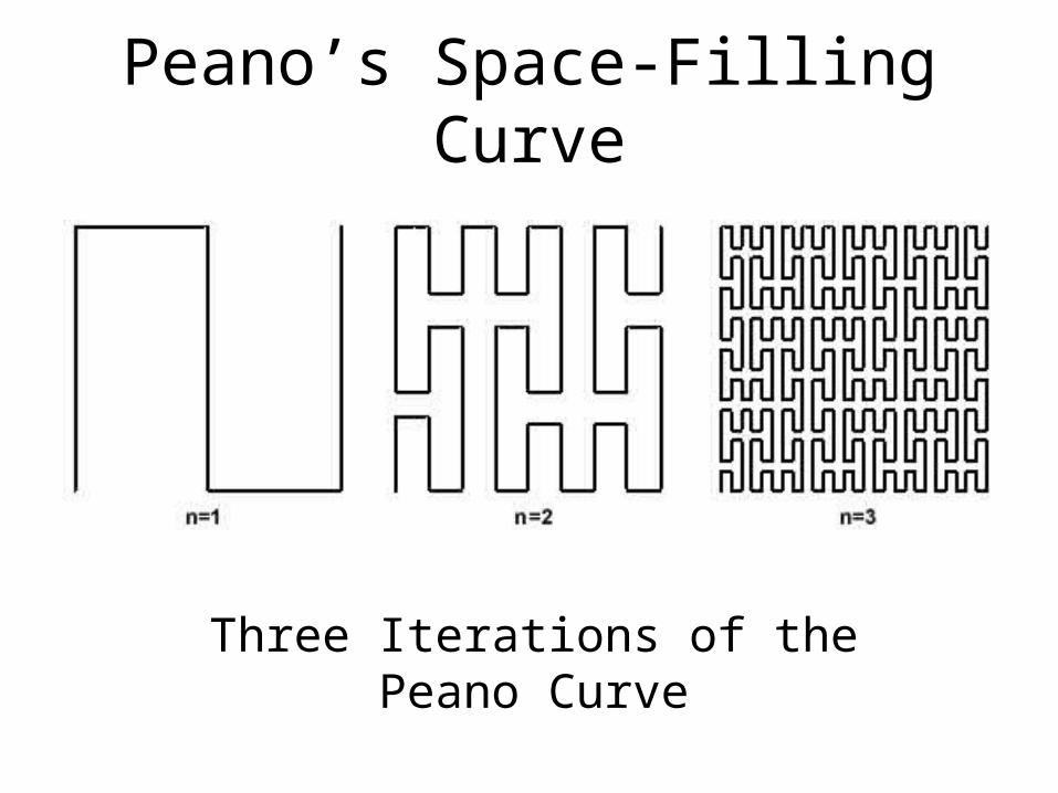
Peano’s Space-Filling Curve
Three Iterations of the Peano Curve
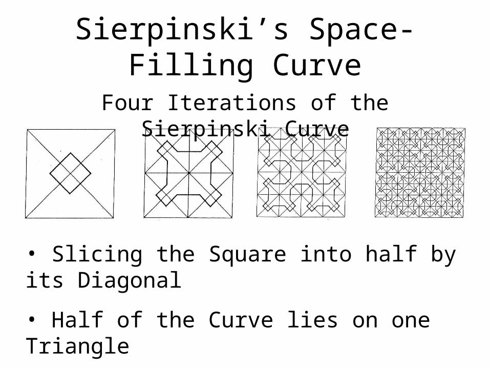
Sierpinski’s Space-Filling Curve
Four Iterations of the Sierpinski Curve
• Slicing the Square into half by its Diagonal
• Half of the Curve lies on one Triangle
• Other half lies on the other Triangle
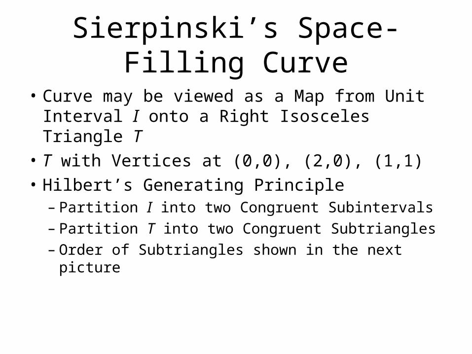
Sierpinski’s Space-Filling Curve
• Curve may be viewed as a Map from Unit Interval I onto a Right Isosceles Triangle T
• T with Vertices at (0,0), (2,0), (1,1)
• Hilbert’s Generating Principle– Partition I into two Congruent Subintervals– Partition T into two Congruent Subtriangles– Order of Subtriangles shown in the next
picture
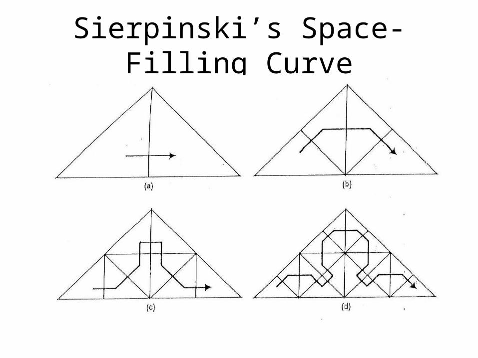
Sierpinski’s Space-Filling Curve
Sierpinski’s Space-Filling Curve
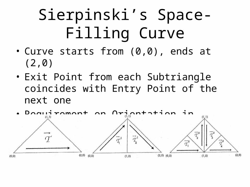
• Curve starts from (0,0), ends at (2,0)• Exit Point from each Subtriangle coincides with
Entry Point of the next one• Requirement on Orientation in Subtriangles
shown in picture below
Recursively Structured Triangular Grids and Sierpinski Curves
– Computational Domain• Right Isosceles Triangle – Starting Cell
– Grid constructed recursively• Split each Triangle Cell into 2 Congruent Subcells• Splitting Repeated until Desired Resolution is
Reached• Grid may be Adaptive – Local Splitting
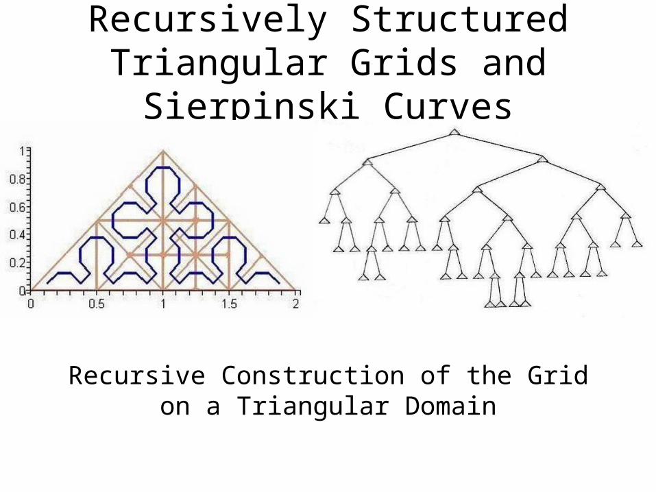
Recursively Structured Triangular Grids and Sierpinski Curves
Recursive Construction of the Grid on a Triangular Domain
Recursively Structured Triangular Grids and Sierpinski Curves
• Cells are in Linear Order on the Sierpinski Curve
• Corresponds to Depth-First Traversal of the Substructuring Tree
• Additional Memory 1 bit per Cell indicating whether– Cell is a Leave, or– Cell is Adaptively Refined
Recursively Structured Triangular Grids and Sierpinski Curves
• Extensions for Flexibility– Several Initial Triangles may be used– Arbitrary Triangles may be used if
• Structure of Recursive Subdivision preserved• One Leg is defined as Tagged Edge and will take
the role of the Hypotenuse
– Tagged Edge can be replaced by a Linear Interpolation of the Boundary (see next picture)
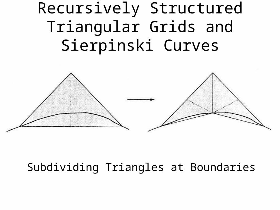
Recursively Structured Triangular Grids and Sierpinski Curves
Subdividing Triangles at Boundaries
Discretization of the PDE
• A Discretization with Linear FE– Generates
• Element Stiffness Matrices• Right Hand Sides
– Accumulates them into Global System of Equations for the Unknowns on the Nodes
• We consider it to be too Memory Consuming
Discretization of the PDE
• Assumption– Stiffness Matrix Computation possible on the
fly, or– Hardcode it into the Software
• Typical for Iterative Solvers– Contain Matrix-Vector Product between
Stiffness Matrix and Unknowns
• Memory used only for storing Grid Structure
Discretization of the PDE
• Classical Node-Oriented Processing– Loop over Unknowns (Nodes on Grid)– Requires Access to all neighbor Nodes– Difficult in a Recursively Structured Grid– Neighbor could be on a Different Subtree
• Our Approach: Cell-Oriented Processing
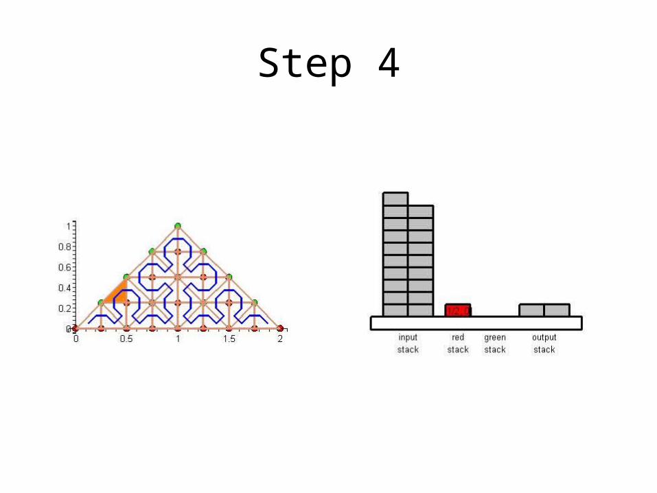
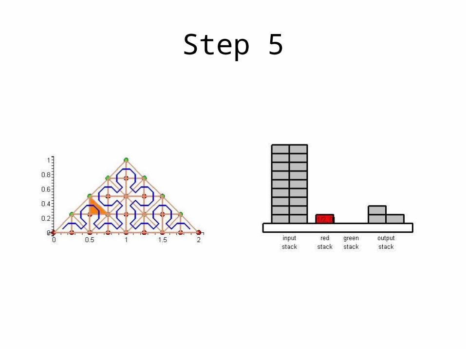
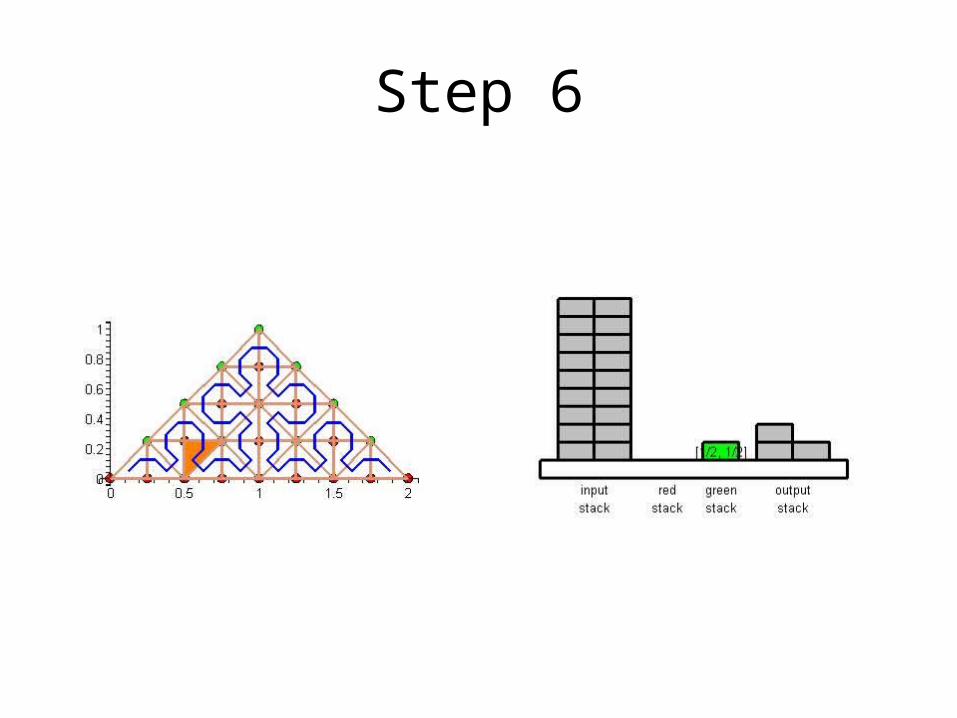
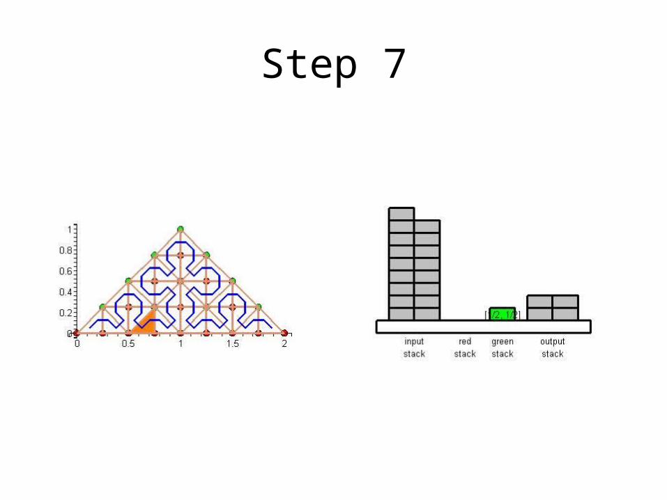
Cache Efficient Processing of the Computational Grid
• Cell-Oriented Processing– Need Access to Unknowns for each Cell– Process Elements along the Sierpinski Curve
• Sierpinski Curve Divides Unknowns into two halves– Left of the Curve: Red Nodes– Right of the Curve: Green Nodes– See picture next
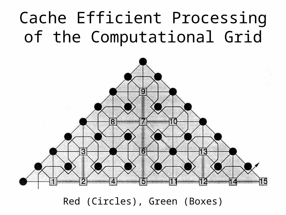
Cache Efficient Processing of the Computational Grid
Red (Circles), Green (Boxes)

Cache Efficient Processing of the Computational Grid
• Access to Unknowns is like Access to a Stack
• Consider Unknowns 5 to 10– During Processing Cells to the Left – Access
in Ascending Order– During Processing Cells to the Right – Access
in Descending Order
• Nodes 8, 9, 10 Placed in turn on Top of the Stack
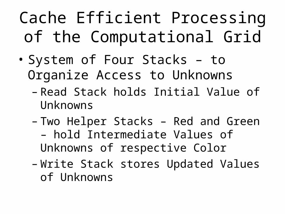
Cache Efficient Processing of the Computational Grid
• System of Four Stacks – to Organize Access to Unknowns– Read Stack holds Initial Value of Unknowns– Two Helper Stacks – Red and Green – hold
Intermediate Values of Unknowns of respective Color
– Write Stack stores Updated Values of Unknowns
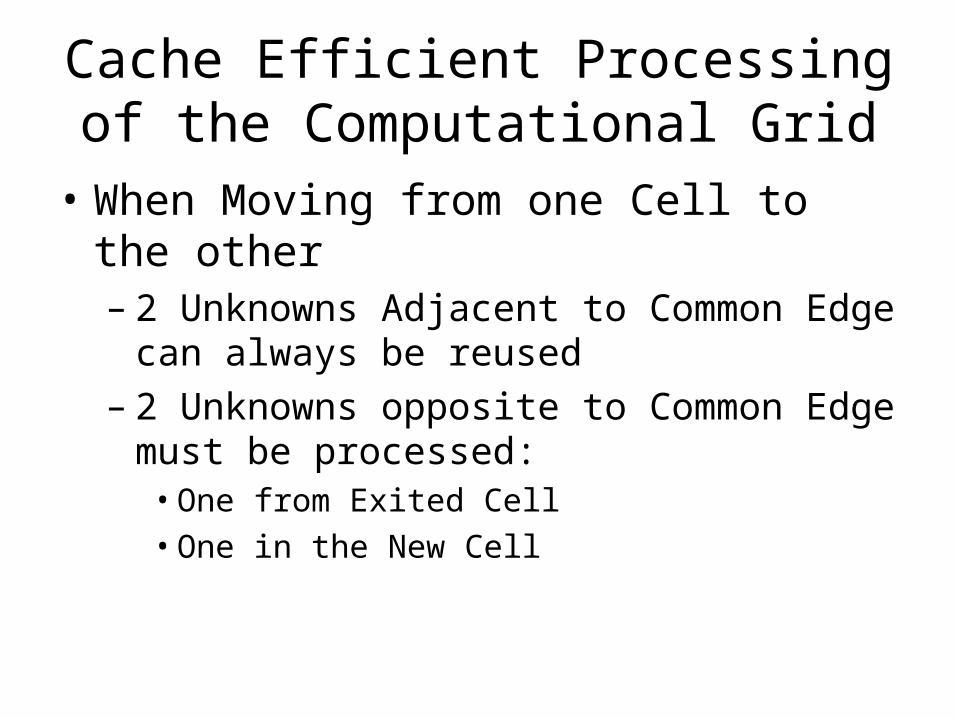
Cache Efficient Processing of the Computational Grid
• When Moving from one Cell to the other– 2 Unknowns Adjacent to Common Edge can
always be reused– 2 Unknowns opposite to Common Edge must
be processed:• One from Exited Cell • One in the New Cell
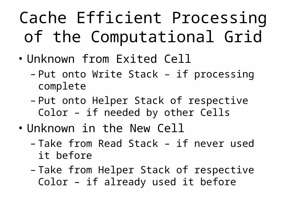
Cache Efficient Processing of the Computational Grid
• Unknown from Exited Cell– Put onto Write Stack – if processing complete– Put onto Helper Stack of respective Color – if
needed by other Cells
• Unknown in the New Cell– Take from Read Stack – if never used it
before– Take from Helper Stack of respective Color –
if already used it before

Cache Efficient Processing of the Computational Grid
• Unknown from Exited Cell– Count number of Accesses – Determine
whether Processing is Complete or not– Determine the Color – Left or Right side of the
Sierpinski Curve ?– Curve Enters and Exits at the 2 Nodes
adjacent to the Hypotenuse– Only 3 possible Scenarios
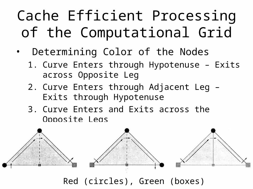
Cache Efficient Processing of the Computational Grid
• Determining Color of the Nodes1. Curve Enters through Hypotenuse – Exits across
Opposite Leg
2. Curve Enters through Adjacent Leg – Exits through Hypotenuse
3. Curve Enters and Exits across the Opposite Legs
Red (circles), Green (boxes)
Cache Efficient Processing of the Computational Grid
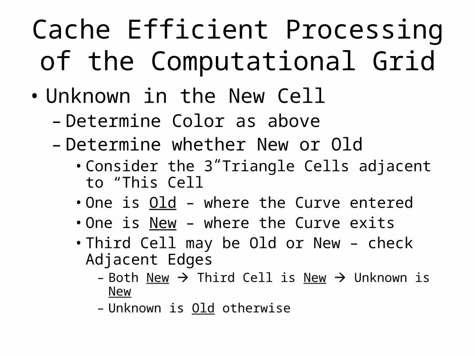
• Unknown in the New Cell– Determine Color as above– Determine whether New or Old
• Consider the 3 Triangle Cells adjacent to “This Cell”
• One is Old – where the Curve entered• One is New – where the Curve exits• Third Cell may be Old or New – check Adjacent
Edges– Both New Third Cell is New Unknown is New– Unknown is Old otherwise
Cache Efficient Processing of the Computational Grid
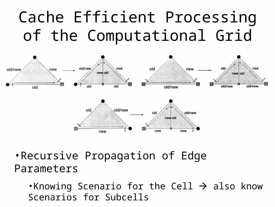
•Recursive Propagation of Edge Parameters
•Knowing Scenario for the Cell also know Scenarios for Subcells
Cache Efficient Processing of the Computational Grid
• Processing of the Grid is managed by a set of 6 Recursive Procedures
• On the Leaves the Discretization-Level Operations are performed
• Example from Maple worksheet is next
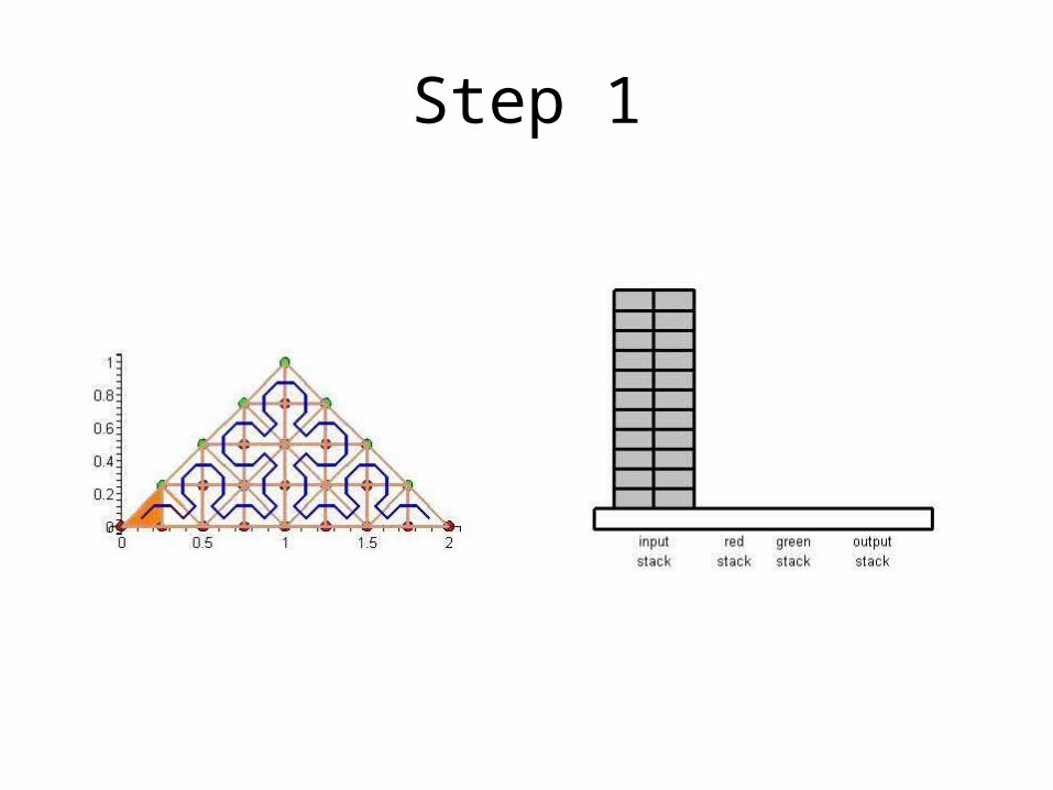
Step 1
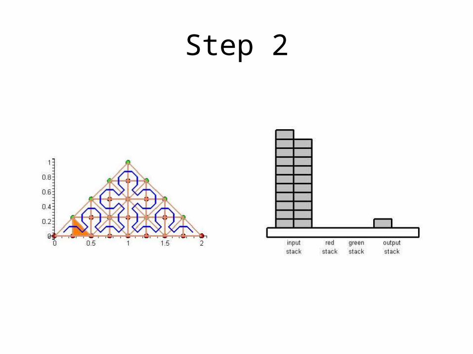
Step 2
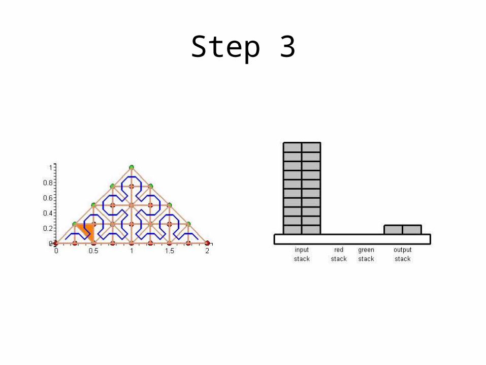
Step 3
Step 4
Step 5
Step 6
Step 7

Step 8
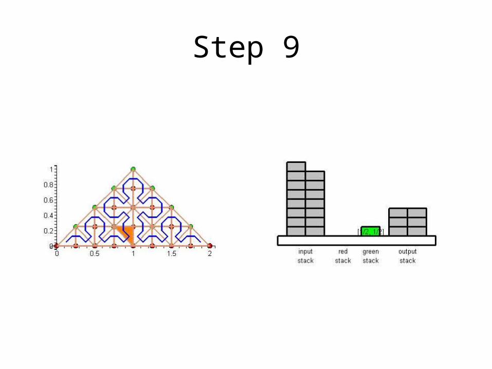
Step 9
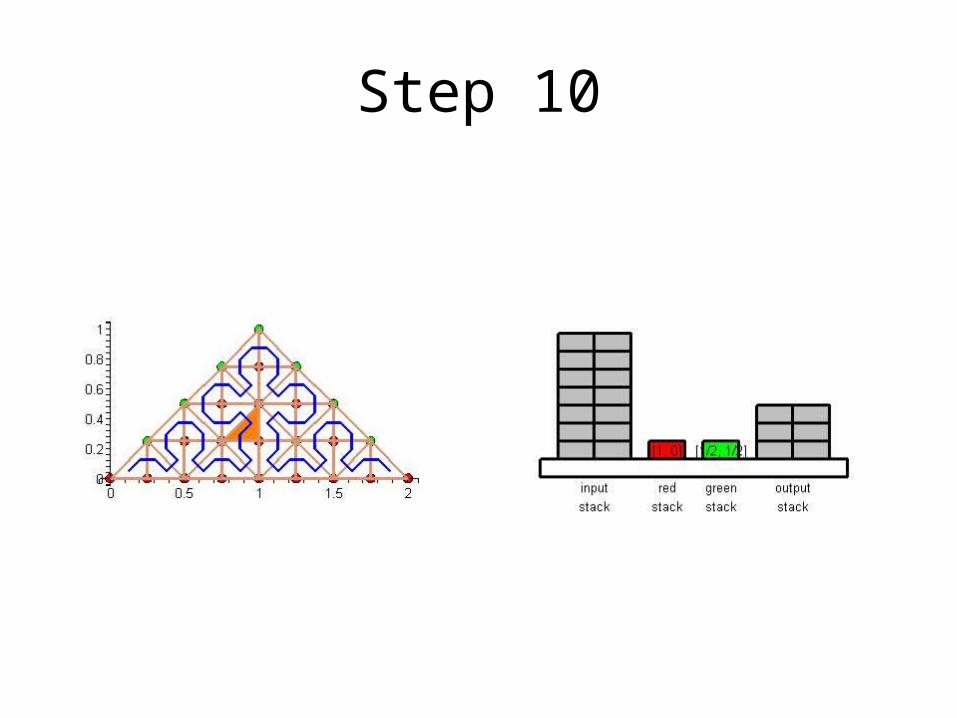
Step 10
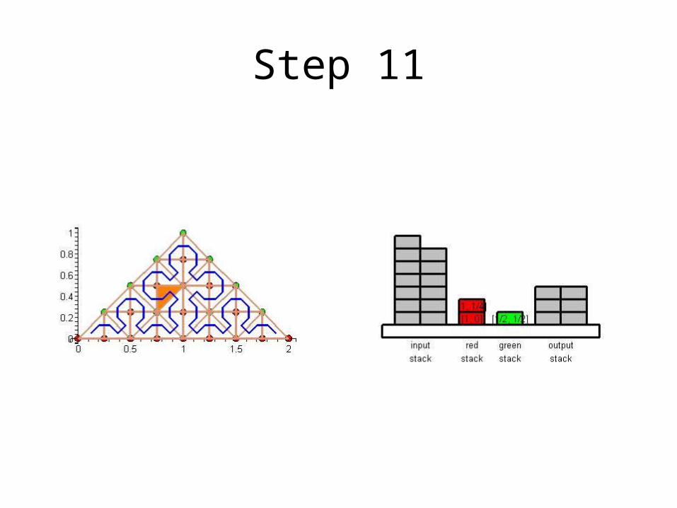
Step 11

Step 12
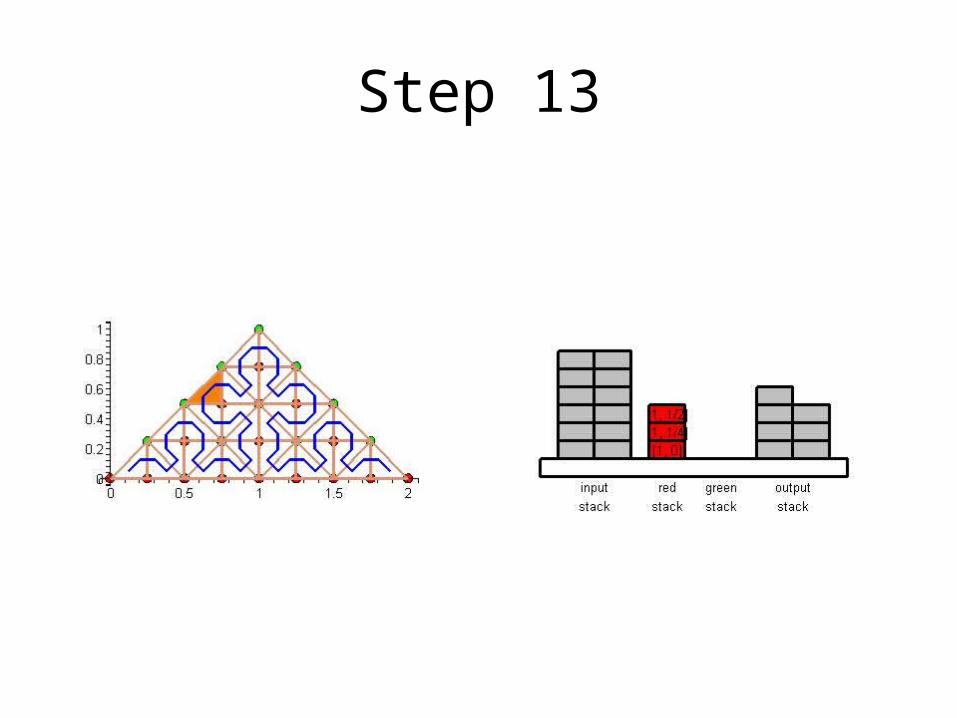
Step 13

Step 14
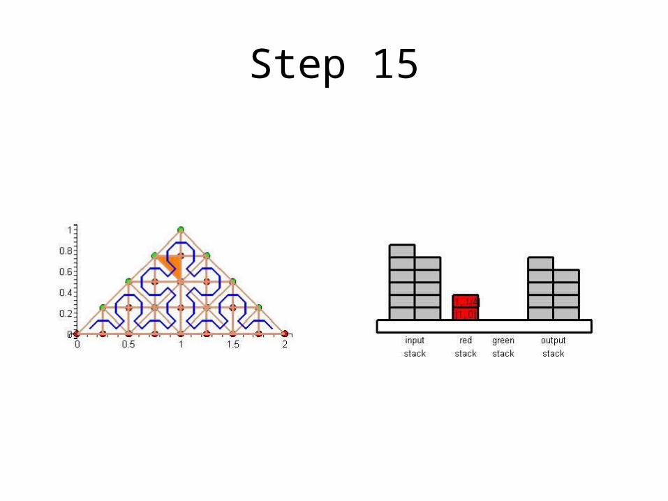
Step 15
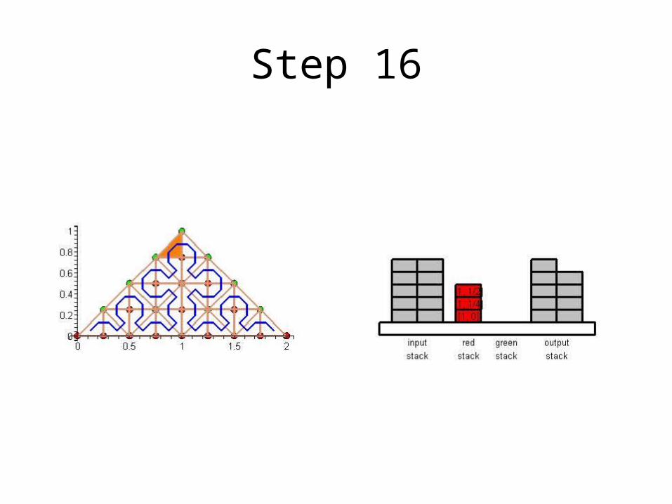
Step 16
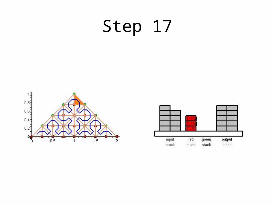
Step 17
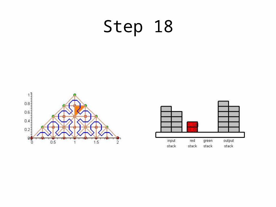
Step 18
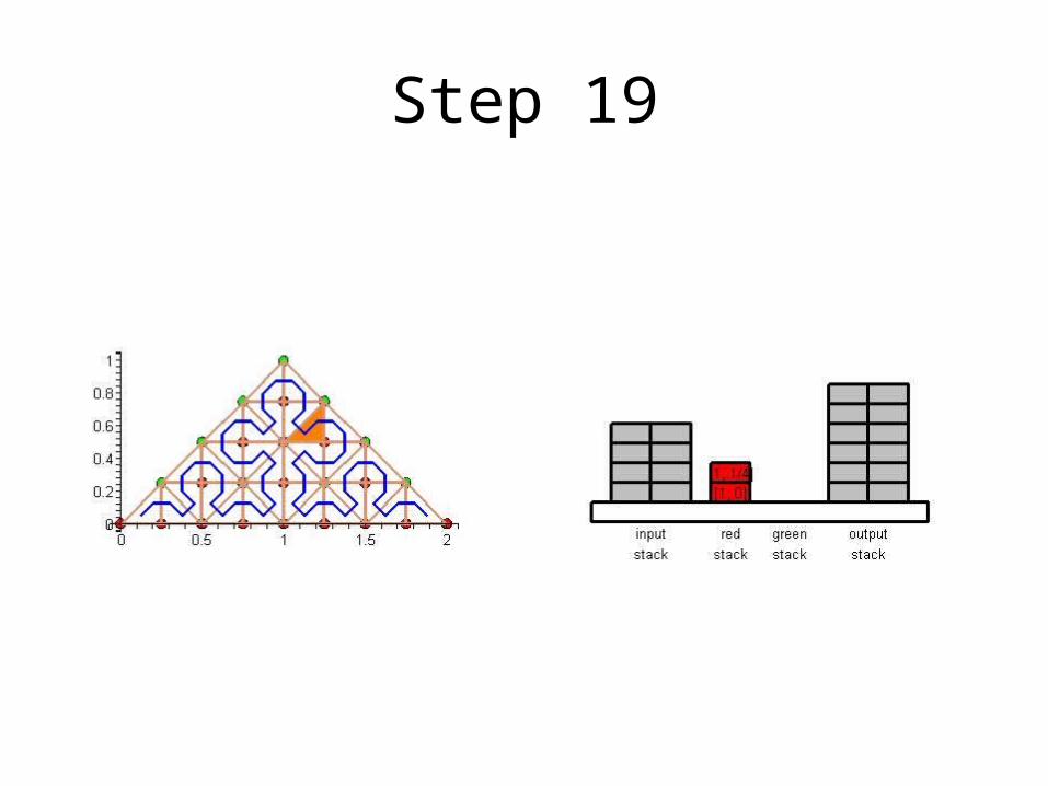
Step 19
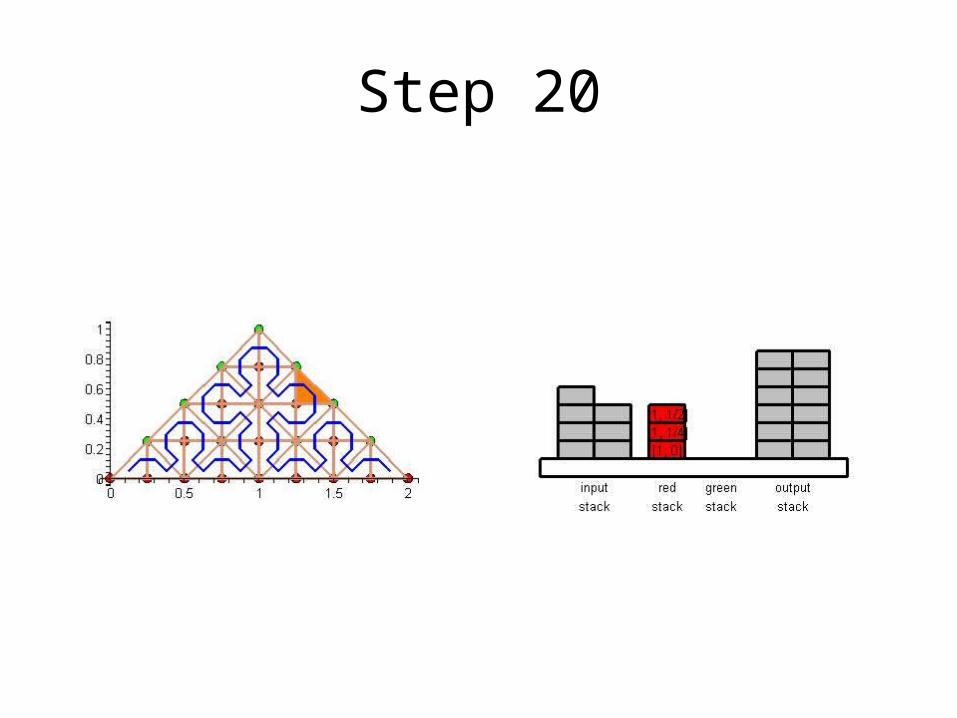
Step 20
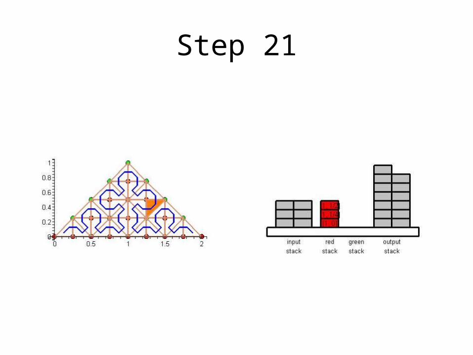
Step 21

Step 22
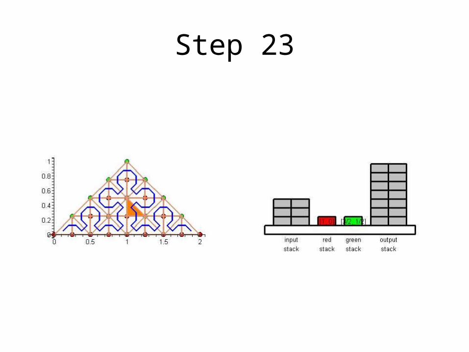
Step 23
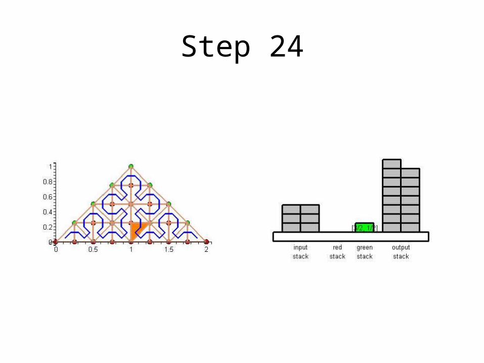
Step 24
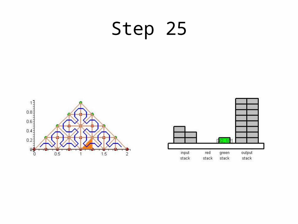
Step 25
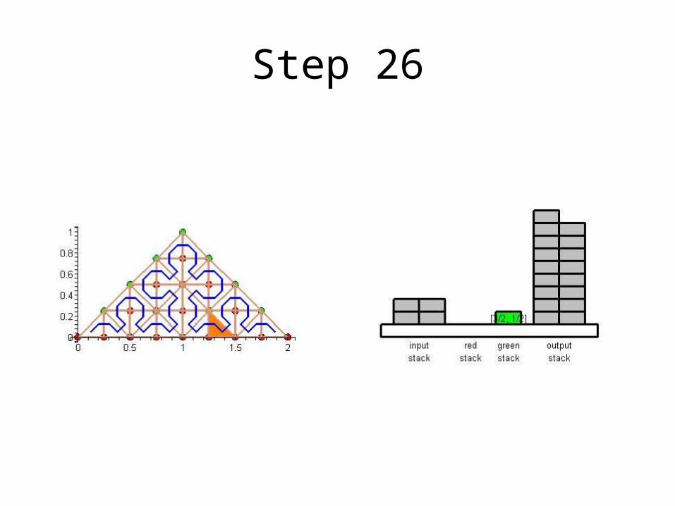
Step 26
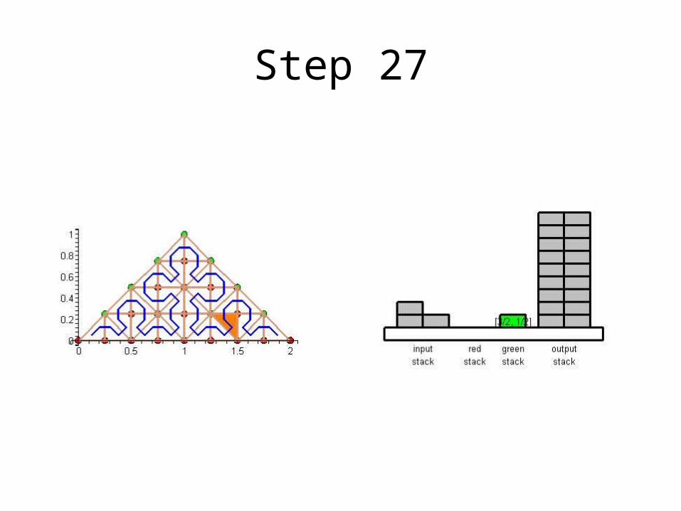
Step 27
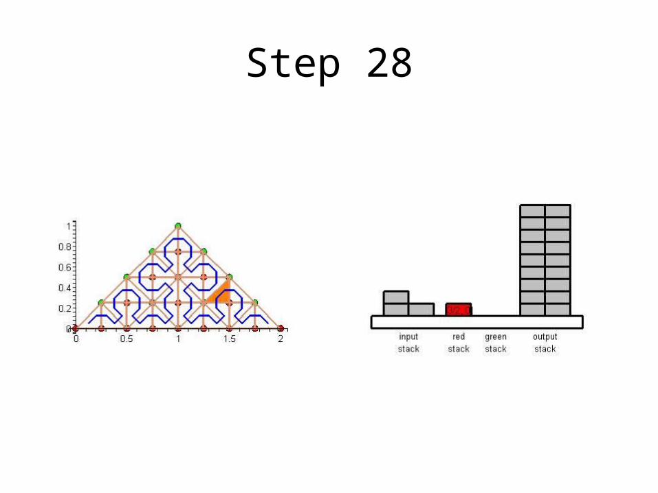
Step 28
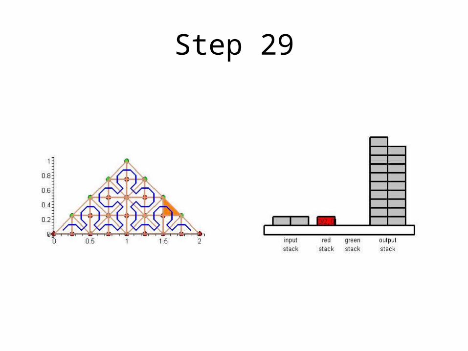
Step 29

Step 30
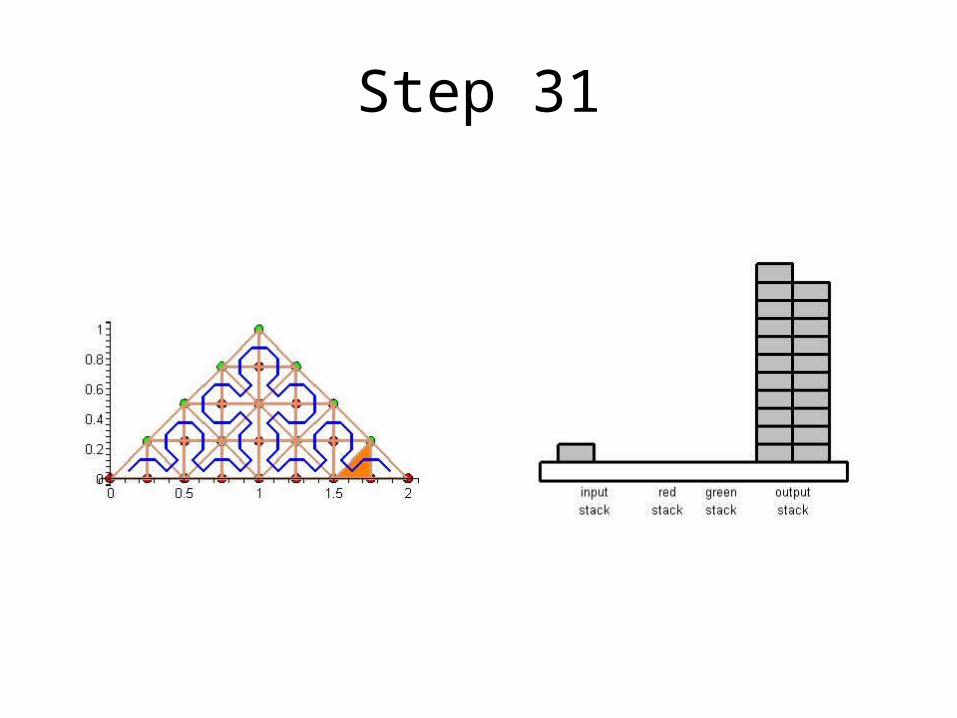
Step 31
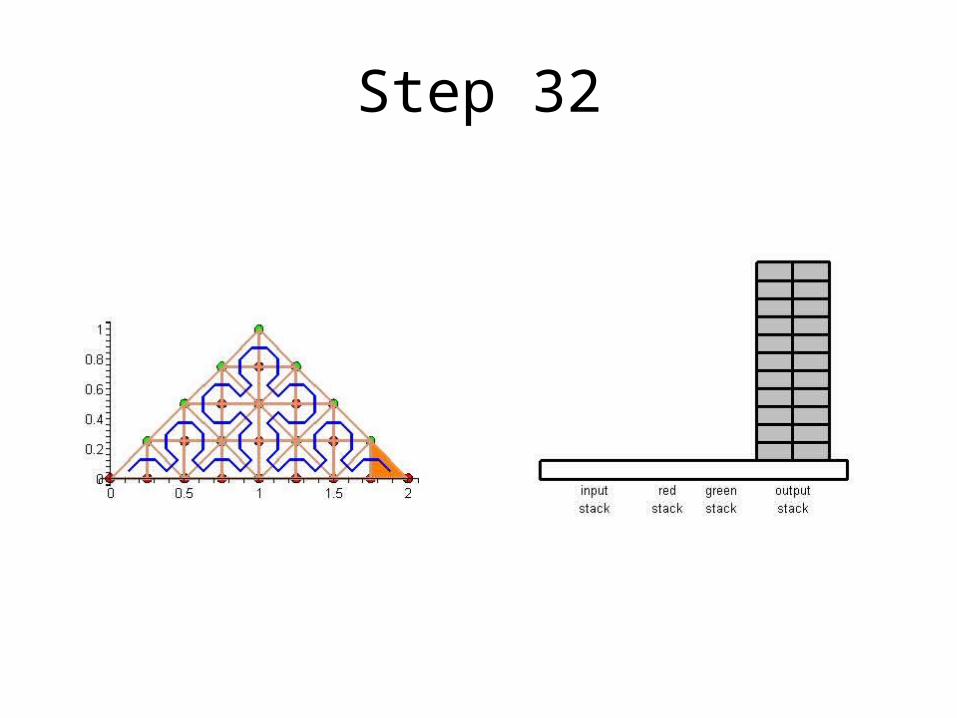
Step 32
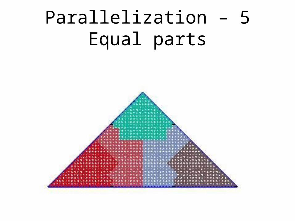
Parallelization – 5 Equal parts
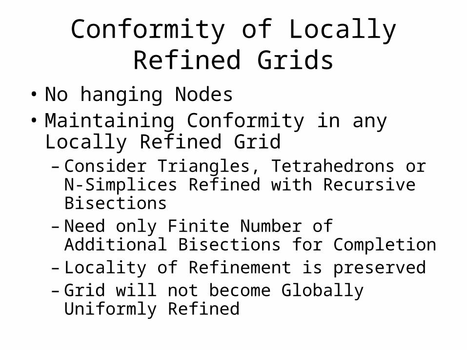
Conformity of Locally Refined Grids
• No hanging Nodes• Maintaining Conformity in any Locally
Refined Grid– Consider Triangles, Tetrahedrons or N-
Simplices Refined with Recursive Bisections– Need only Finite Number of Additional
Bisections for Completion– Locality of Refinement is preserved– Grid will not become Globally Uniformly
Refined
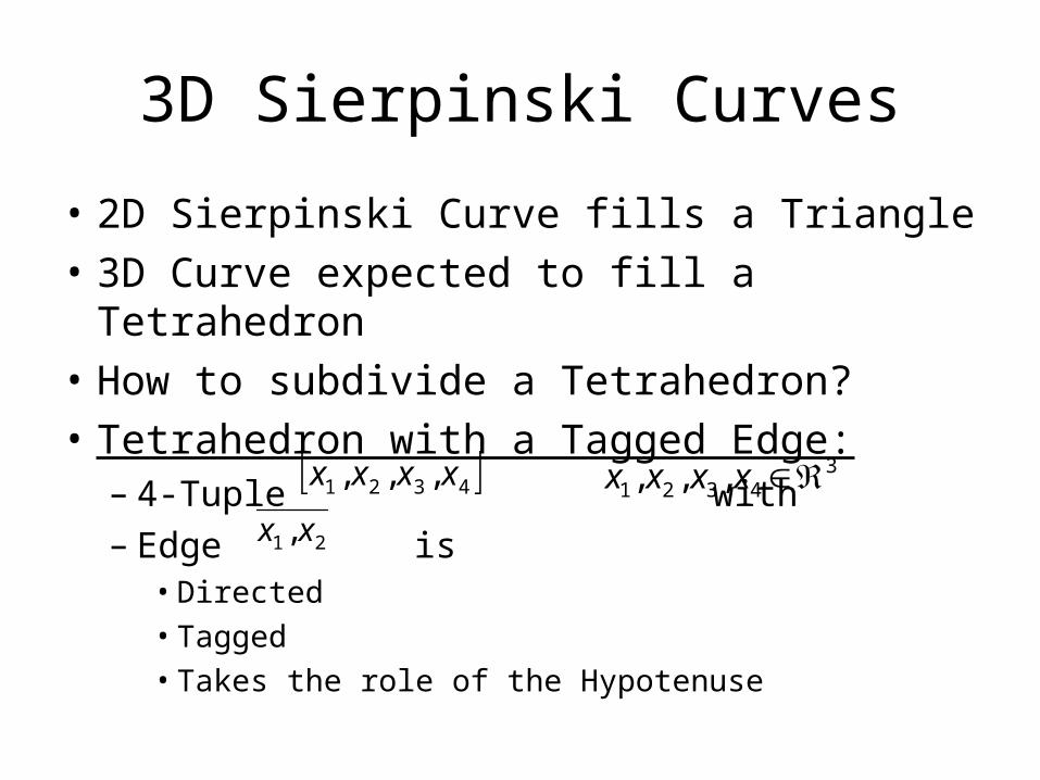
3D Sierpinski Curves
• 2D Sierpinski Curve fills a Triangle
• 3D Curve expected to fill a Tetrahedron
• How to subdivide a Tetrahedron?
• Tetrahedron with a Tagged Edge:– 4-Tuple with– Edge is
• Directed• Tagged• Takes the role of the Hypotenuse
4321 ,,, xxxx 34321 ,,, xxxx
21 , xx
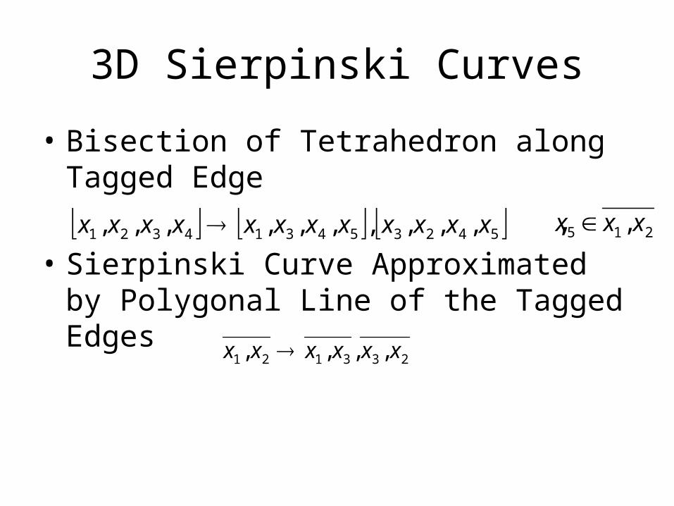
3D Sierpinski Curves
• Bisection of Tetrahedron along Tagged Edge
,
• Sierpinski Curve Approximated by Polygonal Line of the Tagged Edges
542354314321 ,,,,,,,,,, xxxxxxxxxxxx 215 , xxx
233121 ,,,, xxxxxx
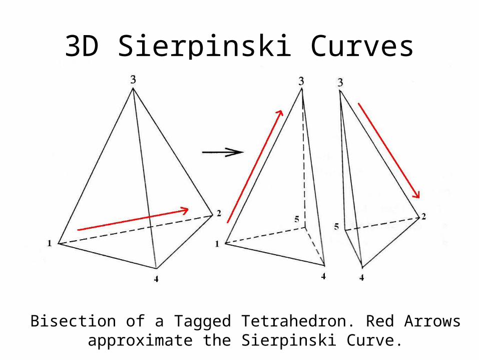
3D Sierpinski Curves
Bisection of a Tagged Tetrahedron. Red Arrows approximate the Sierpinski Curve.
Conclusion
• Algorithm Efficiently generates and processes Adaptive Triangular Grids
• Memory Requirement is minimal
• Hope to achieve Computational Speed competitive with Algorithms based on Regular Grids
• Extension to 3D is currently subject to research

Questions?
???
Thank You!