Embed Size (px)
Citation preview
Efficient Semiparametric Seemingly Unrelated
Quantile Regression Estimation
Sung Jae Jun∗and Joris Pinkse†
The Pennsylvania State Universityand
The Center for the Study of Auctions, Procurements and Competition Policy
June 2008
Abstract
We propose an efficient semiparametric estimator for the coefficients of a multivariate linear re-gression model — with a conditional quantile restriction for each equation — in which the conditionaldistributions of errors given regressors are unknown. The procedure can be used to estimate multipleconditional quantiles of the same regression relationship. The proposed estimator is asymptotically asefficient as if the true optimal instruments were known. Simulation results suggest that the estimationprocedure works well in practice and dominates an equation–by–equation efficiency correction if theerrors are dependent conditional on the regressors.
∗(corresponding author) Department of Economics, The Pennsylvania State University, 608 Kern Graduate Building,University Park PA 16802, [email protected]
†[email protected] We thank the coeditor, two anonymous referees and participants at the Carnegie Mellon departmentalseminar and Ari Kang for their useful suggestions. We thank the Human Capital Foundation for their support.
1
1 Introduction
1 Introduction
We propose an efficient semiparametric estimator for the coefficients of a multivariate linear regression
model — with a conditional quantile restriction for each equation — in which the conditional distributions
of errors given regressors are unknown. The procedure can be used to estimate multiple conditional
quantiles of the same regression relationship. The proposed estimator is asymptotically as efficient as if
the true optimal instruments were known. Simulation results suggest that the estimation procedure works
well in practice and dominates an equation–by–equation efficiency correction if the errors are dependent
conditional on the regressors.
The proposed method entails the nonparametric estimation of optimal instruments for a set of moment
conditions corresponding to the conditional quantiles of interest and subsequently using these estimated
optimal instruments to obtain the efficient quantile estimates. Two–step efficiency corrections like this go
back to at least Aitken (1935), and semiparametric corrections like ours have been around for a while, also.
Carroll (1982), Delgado (1992) and Robinson (1987) show that by estimating the conditional error variance
function nonparametrically the same asymptotic variance can be achieved as with (infeasible) GLS. Newey
(1990, 1993) proposes methods for estimating optimal instruments nonparametrically, thereby allowing for
multivariate regressions and ones with endogenous regressors. Pinkse (2006) introduces a method which
addresses the curse of dimensionality associated with the nonparametric estimation of functions with
many arguments. Finally, Zhao (2001), Whang (2006), and Komunjer and Vuong (2006) propose efficiency
corrections for the univariate quantile regression model.
Like all of the above semiparametric estimators ours relies on the availability of a√n–consistent first
round estimator; a natural choice is the standard quantile regression estimator. A problem with such a
two–step procedure is that the first round estimation error, while asymptotically absent, can be such that
correction is not worthwhile in small samples. This is especially true when the number of regressors is large
due to the fact that nonparametric estimators of high–dimensional functions are notoriously inaccurate.
Please note however, that our correction does not require (nor do we establish) pointwise consistent esti-
mation of the optimal instruments. Further, the uncorrected estimates are special cases of the correction
2
1 Introduction
procedure for particular values of the input parameters of the semiparametric method, but we offer no
procedure for the optimal selection of the input parameters. Earlier work (Pinkse, 2006) and some exper-
imentation (not reported) suggest that our procedure is comparatively insensitive to the choice of input
parameters.
This paper contains several theoretical innovations. While Newey (1990, 1993) allows for multiple equa-
tions to be estimated jointly, his results do not cover the current case because of nondifferentiability issues.
Zhao (2001), Whang (2006) and Komunjer and Vuong (2006) propose estimators for the single equation
case. In the single equation case the nuisance function is just conditional error density at zero instead of
the product of a matrix and the inverse of another matrix, as is the case here. Whang (2006) and Komunjer
and Vuong (2006) achieve the semiparametric efficiency bound (the latter for time series) by optimizing an
objective function involving a series expansion of the nuisance function; the nondifferentiability problems
we solve do not arise then.
Our paper is closer to Zhao (2001) in that we use a nonparametric plugin estimator, but they differ in
several dimensions. Zhao’s results only cover the single–equation case and are not readily generalized to
the multivariate case. Further, Zhao uses a less primitive technical condition on the construction of the
weights, while we have specifically opted for nearest neighbor estimation; we believe that nearest neighbor
weights satisfy Zhao’s condition. A final difference concerns the way in which the first step estimation
error is addressed. For both methods (Zhao’s and ours) first step estimates enter the second step via
a nondifferentiable function. Zhao proposes two distinct procedures to address this problem. The first
procedure entails sample splitting, i.e. using half the data to get the first step estimator to be used as a
plug–in in the second step for the second half of the data and vice versa. This procedure does not make a
difference asymptotically, but is less attractive due to its inherent (finite sample) inefficiency. His second
procedure assumes that the first step estimator has a certain Bahadur representation, which we believe is
likely to hold in practice.
We do not know whether Zhao’s methods can be extended to the multivariate case. Instead, we follow
a new line of proof which neither entails sample–splitting nor does it require any assumptions on the first
step estimator beyond a convergence rate. The new proof (contained in the last two lemmas of appendix C
3
2 Model and Estimator
and using lemma 2 of appendix A) entails ratcheting up of the established uniform convergence rate of the
feasible estimator of the moment condition and the feasible estimator of the parameter vector of interest
alternately. This method of proof has uses that go well beyond the particular problem at hand or indeed
differentiability problems or ones involving nonparametric estimation.
To compute our estimates we propose procedures involving solving standard linear programming (LP)
problems possibly combined with taking a Newton step. The procedure is guaranteed to yield estimates
satisfying our constraints — we prove this — and does so fast; computing the nonparametric weights takes
the most time. The Matlab code is available from the authors on request.
The outline of the paper is as follows. In section 2 we introduce the setup and define our estimator.
Section 3 contains the theoretical results for our estimator, whose computation and performance are studied
in section 4.
2 Model and Estimator
Let yi, Xi be an i.i.d. sequence for which
Q(yi|Xi) = X ′iθ0 a.s., i = 1, . . . , n, (1)
or equivalently,
yi = X ′iθ0 + ui, Q(ui|Xi) = 0 a.s., i = 1, . . . , n, (2)
where Q denotes the vector of quantiles of interest, yi ∈ Rd, and Xi ∈ RK×d with d the number of regression
equations and K the total number of unknown regression coefficients.
The restriction that the same θ0–vector occurs in all regression equations is not restrictive, because we
can make the choices Xi = ⊕dj=1xij and θ0 = [θ′01, . . . , θ
′0d]
′,1 resulting in
yij = x′ijθ0j + uij , i = 1, . . . , n; j = 1, . . . , d. (3)
Note that (1) allows for linear cross–equation restrictions on the parameters.1⊕ denotes ‘matrix direct sum,’ i.e. the result is like a block–diagonal matrix with nonsquare diagonal blocks xij .
4
2 Model and Estimator
An assumption implicit in (1) is that Q(yij |xi`, xij) = Q(yij |xij) a.s.. This is where part of the efficiency
gain originates; it is akin to an orthogonality condition between regressors and errors across equations in
the mean regression case. A more detailed discussion of this and related issues follows further below.
It is possible to choose yij = yi`, xij = xi`, j 6= `, for all i in (3) if different regression quantiles of the
same regression relationship are desired. Assuming multiple quantiles of the same relationship to all be
linear, however, imposes strong restrictions on the types of dependence between errors and regressors that
can be accomodated and a procedure that exploits such restrictions will likely work better in practice than
the more general procedure proposed here; a more fruitful avenue would be to estimate the median and
mean jointly, a possibility not covered by our results.
We now formulate an infeasible efficient estimation procedure for θ0. Let si(θ) = I(yi ≤ X ′iθ) − τ ,
where τ is the vector indicating which quantiles are desired (a vector with values 0.5 in case of the median)
and I is the indicator function, where for any v ∈ Rdv , I(v) = [I(v1), . . . , I(vdv)]′. Then the conditional
moment condition is E(si|Xi) = 0 a.s.. (si = si(θ0)). The corresponding optimal unconditional moment
conditions are
E(Aisi) = 0, (4)
where Ai = S′iT−1i with
Si = FiX′i, Fi = ⊕d
j=1fuij |Xi(0), Ti = E(sis
′i|Xi).2 (5)
The asymptotic variance of an infeasible estimator θI based on (4) will later be shown to be V = Ψ−1 with
Ψ = E(A1s1s′1A
′1) = E(S′1T
−11 S1). (6)
The proposed procedure yields a natural efficiency improvement over equation–by–equation estimation
when there are cross–equation restrictions on the regression coefficients.
Absent such restrictions, the intuition for the nature of the efficiency improvement can be understood
by comparing four estimators. The first estimator is θSI = [θ′SI1, . . . , θ′SId]
′, where θSIj is the traditional
2 These unconditional moments are optimal in the sense that estimators based on them achieve the semiparametric efficiencybounds. See e.g. Chamberlain (1987), Newey (1993).
5
2 Model and Estimator
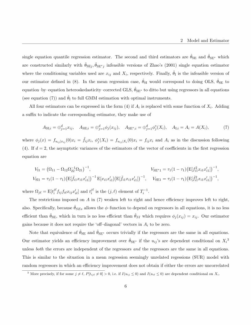
single equation quantile regression estimator. The second and third estimators are θSE and θSE∗ which
are constructed similarly with θSEj , θSE∗j infeasible versions of Zhao’s (2001) single equation estimator
where the conditioning variables used are xij and Xi, respectively. Finally, θI is the infeasible version of
our estimator defined in (8). In the mean regression case, θSI would correspond to doing OLS, θSE to
equation–by–equation heteroskedasticity–corrected GLS, θSE∗ to ditto but using regressors in all equations
(see equation (7)) and θI to full GMM estimation with optimal instruments.
All four estimators can be expressed in the form (4) if Ai is replaced with some function of Xi. Adding
a suffix to indicate the corresponding estimator, they make use of
ASI;i = ⊕dj=1xij , ASE;i = ⊕d
j=1φj(xij), ASE∗;i = ⊕dj=1φ
∗j (Xi), AI;i = Ai = A(Xi), (7)
where φj(x) = fuij |xij(0)xi = fijxi, φ∗j (Xi) = fuij |Xi
(0)xi = fijxi and Ai as in the discussion following
(4). If d = 2, the asymptotic variances of the estimators of the vector of coefficients in the first regression
equation are
VI1 =(Ω11 − Ω12Ω−1
22 Ω21
)−1, VSE∗1 = τ1(1− τ1)
(E[f2
i1xi1x′i1]
)−1,
VSI1 = τ1(1− τ1)(E[fi1xi1x
′i1]
)−1 E[xi1x′i1]
(E[fi1xi1x
′i1]
)−1, VSE1 = τ1(1− τ1)
(E[f2
i1xi1x′i1]
)−1,
where Ωj` = E[tj`i fijfi`xijx′i`] and tj`i is the (j, `) element of T−1
i .
The restrictions imposed on A in (7) weaken left to right and hence efficiency improves left to right,
also. Specifically, because θSEs allows the φ–function to depend on regressors in all equations, it is no less
efficient than θSE, which in turn is no less efficient than θSI which requires φj(xij) = xij . Our estimator
gains because it does not require the ‘off–diagonal’ vectors in Ai to be zero.
Note that equivalence of θSE and θSE∗ occurs trivially if the regressors are the same in all equations.
Our estimator yields an efficiency improvement over θSE∗ if the uij ’s are dependent conditional on Xi3
unless both the errors are independent of the regressors and the regressors are the same in all equations.
This is similar to the situation in a mean regression seemingly unrelated regessions (SUR) model with
random regressors in which an efficiency improvement does not obtain if either the errors are uncorrelated3 More precisely, if for some j 6= `, P [tij` 6= 0] > 0, i.e. if I(uij ≤ 0) and I(ui` ≤ 0) are dependent conditional on Xi.
6
2 Model and Estimator
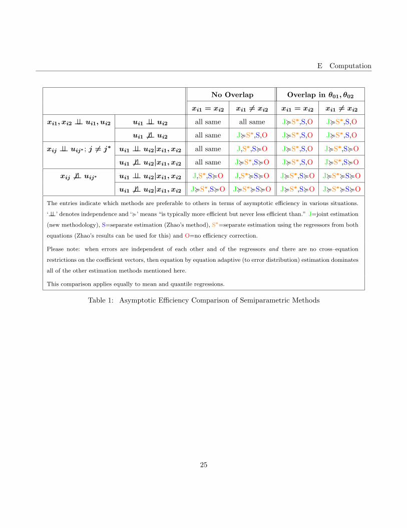
conditional on the regressors or the regressors are identical and independent of the errors.4 Table 1 contains
full details of when efficiency improvements obtain in the quantile model for the various estimators.
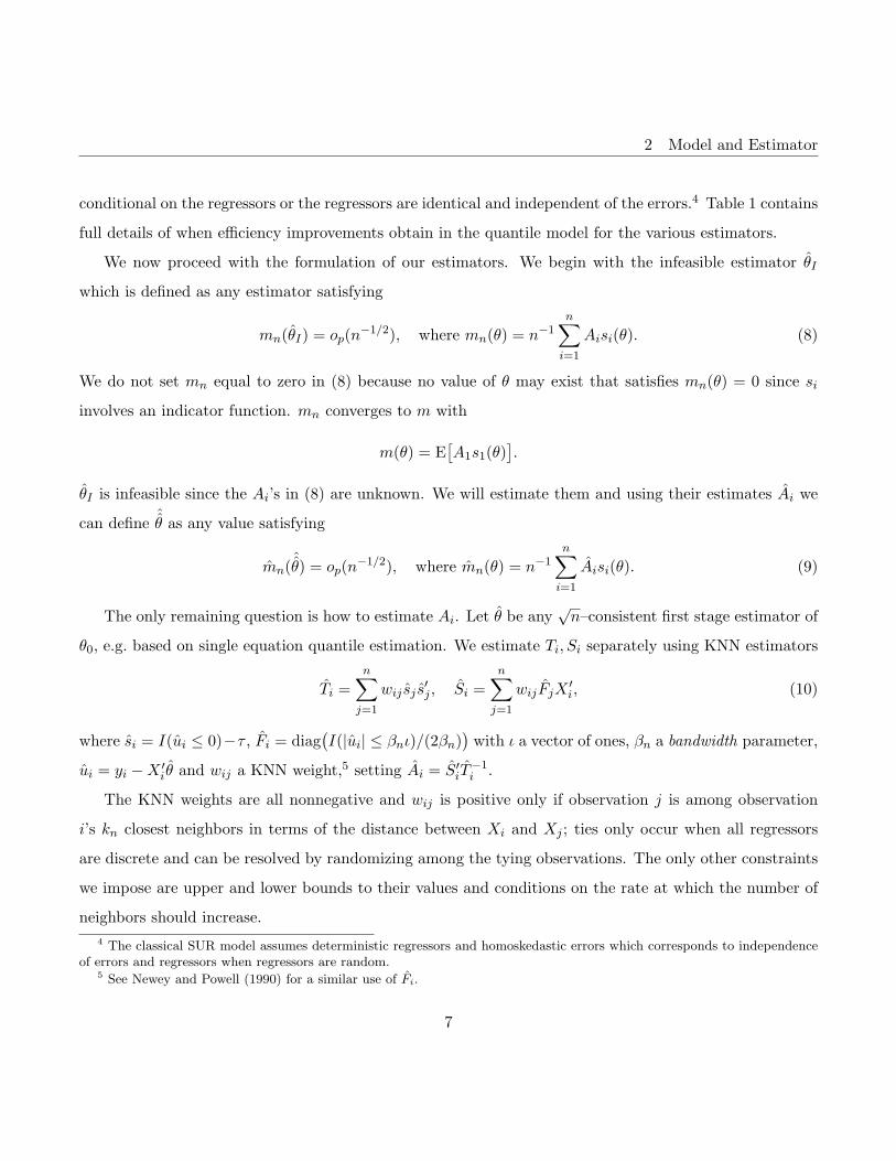
We now proceed with the formulation of our estimators. We begin with the infeasible estimator θI
which is defined as any estimator satisfying
mn(θI) = op(n−1/2), where mn(θ) = n−1n∑
i=1
Aisi(θ). (8)
We do not set mn equal to zero in (8) because no value of θ may exist that satisfies mn(θ) = 0 since si
involves an indicator function. mn converges to m with
m(θ) = E[A1s1(θ)
].
θI is infeasible since the Ai’s in (8) are unknown. We will estimate them and using their estimates Ai we
can define ˆθ as any value satisfying
mn(ˆθ) = op(n−1/2), where mn(θ) = n−1n∑
i=1
Aisi(θ). (9)
The only remaining question is how to estimate Ai. Let θ be any√n–consistent first stage estimator of
θ0, e.g. based on single equation quantile estimation. We estimate Ti, Si separately using KNN estimators
Ti =n∑
j=1
wij sj s′j , Si =
n∑j=1
wijFjX′i, (10)
where si = I(ui ≤ 0)−τ , Fi = diag(I(|ui| ≤ βnι)/(2βn)
)with ι a vector of ones, βn a bandwidth parameter,
ui = yi −X ′iθ and wij a KNN weight,5 setting Ai = S′iT
−1i .
The KNN weights are all nonnegative and wij is positive only if observation j is among observation
i’s kn closest neighbors in terms of the distance between Xi and Xj ; ties only occur when all regressors
are discrete and can be resolved by randomizing among the tying observations. The only other constraints
we impose are upper and lower bounds to their values and conditions on the rate at which the number of
neighbors should increase.4 The classical SUR model assumes deterministic regressors and homoskedastic errors which corresponds to independence
of errors and regressors when regressors are random.5 See Newey and Powell (1990) for a similar use of Fi.
7
3 Results
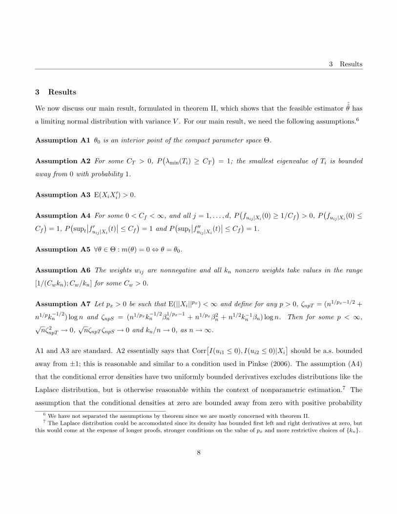
3 Results
We now discuss our main result, formulated in theorem II, which shows that the feasible estimator ˆθ has
a limiting normal distribution with variance V . For our main result, we need the following assumptions.6
Assumption A1 θ0 is an interior point of the compact parameter space Θ.
Assumption A2 For some CT > 0, P(λmin(Ti) ≥ CT
)= 1; the smallest eigenvalue of Ti is bounded
away from 0 with probability 1.
Assumption A3 E(XiX′i) > 0.
Assumption A4 For some 0 < Cf <∞, and all j = 1, . . . , d, P(fuij |Xi
(0) ≥ 1/Cf
)> 0, P
(fuij |Xi
(0) ≤
Cf
)= 1, P
(supt
∣∣f ′uij |Xi(t)
∣∣ ≤ Cf
)= 1 and P
(supt
∣∣f ′′uij |Xi(t)
∣∣ ≤ Cf
)= 1.
Assumption A5 ∀θ ∈ Θ : m(θ) = 0 ⇔ θ = θ0.
Assumption A6 The weights wij are nonnegative and all kn nonzero weights take values in the range
[1/(Cwkn);Cw/kn] for some Cw > 0.
Assumption A7 Let px > 0 be such that E(||Xi||px) <∞ and define for any p > 0, ζnpT = (n1/px−1/2 +
n1/pk−1/2n ) log n and ζnpS = (n1/pxk
−1/2n β
1/px−1n + n1/pxβ2
n + n1/2k−1n βn) log n. Then for some p < ∞,
√nζ2
npT → 0,√nζnpT ζnpS → 0 and kn/n→ 0, as n→∞.
A1 and A3 are standard. A2 essentially says that Corr[I(ui1 ≤ 0), I(ui2 ≤ 0)|Xi
]should be a.s. bounded
away from ±1; this is reasonable and similar to a condition used in Pinkse (2006). The assumption (A4)
that the conditional error densities have two uniformly bounded derivatives excludes distributions like the
Laplace distribution, but is otherwise reasonable within the context of nonparametric estimation.7 The
assumption that the conditional densities at zero are bounded away from zero with positive probability6 We have not separated the assumptions by theorem since we are mostly concerned with theorem II.7 The Laplace distribution could be accomodated since its density has bounded first left and right derivatives at zero, but
this would come at the expense of longer proofs, stronger conditions on the value of px and more restrictive choices of kn.
8
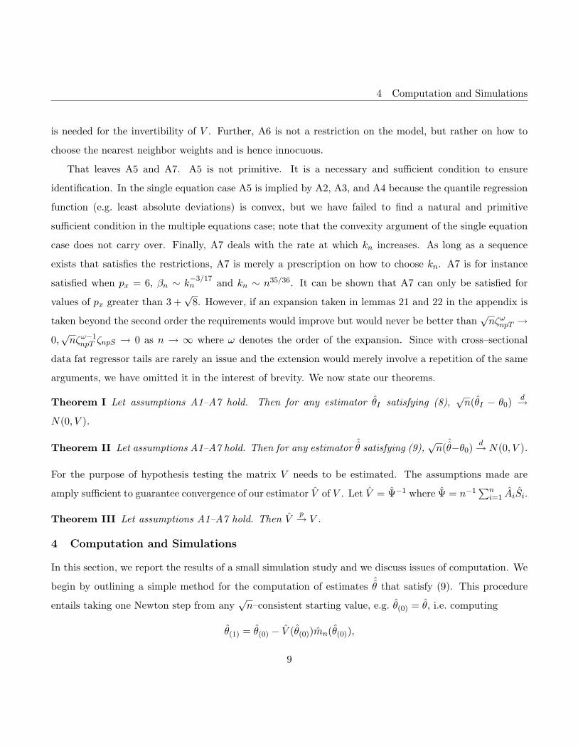
4 Computation and Simulations
is needed for the invertibility of V . Further, A6 is not a restriction on the model, but rather on how to
choose the nearest neighbor weights and is hence innocuous.
That leaves A5 and A7. A5 is not primitive. It is a necessary and sufficient condition to ensure
identification. In the single equation case A5 is implied by A2, A3, and A4 because the quantile regression
function (e.g. least absolute deviations) is convex, but we have failed to find a natural and primitive
sufficient condition in the multiple equations case; note that the convexity argument of the single equation
case does not carry over. Finally, A7 deals with the rate at which kn increases. As long as a sequence
exists that satisfies the restrictions, A7 is merely a prescription on how to choose kn. A7 is for instance
satisfied when px = 6, βn ∼ k−3/17n and kn ∼ n35/36. It can be shown that A7 can only be satisfied for
values of px greater than 3 +√
8. However, if an expansion taken in lemmas 21 and 22 in the appendix is
taken beyond the second order the requirements would improve but would never be better than√nζω
npT →
0,√nζω−1
npT ζnpS → 0 as n → ∞ where ω denotes the order of the expansion. Since with cross–sectional
data fat regressor tails are rarely an issue and the extension would merely involve a repetition of the same
arguments, we have omitted it in the interest of brevity. We now state our theorems.
Theorem I Let assumptions A1–A7 hold. Then for any estimator θI satisfying (8),√n(θI − θ0)
d→
N(0, V ).
Theorem II Let assumptions A1–A7 hold. Then for any estimator ˆθ satisfying (9),
√n(ˆθ−θ0)
d→ N(0, V ).
For the purpose of hypothesis testing the matrix V needs to be estimated. The assumptions made are
amply sufficient to guarantee convergence of our estimator V of V . Let V = Ψ−1 where Ψ = n−1∑n
i=1 AiSi.
Theorem III Let assumptions A1–A7 hold. Then Vp→ V .
4 Computation and Simulations
In this section, we report the results of a small simulation study and we discuss issues of computation. We
begin by outlining a simple method for the computation of estimates ˆθ that satisfy (9). This procedure
entails taking one Newton step from any√n–consistent starting value, e.g. θ(0) = θ, i.e. computing
θ(1) = θ(0) − V (θ(0))mn(θ(0)),
9
4 Computation and Simulations
This is a familiar procedure, where only the nondifferentiability issues provide minor complications; com-
plications which were largely addressed in the earlier theorems.
Theorem IV Let assumptions A1–A7 hold. Then θ(1) solves (9).
Experience based on our simulations suggests that the above–described procedure often leads to an
increase of the value of || ˆmn||, and the resulting estimate θ(1) does not behave as well as the theory
predicts. We therefore propose an alternative procedure to ensure that (9) remains satisfied, but it only
works when there are no cross–equation restrictions on the coefficients.
Consider the case of two equations. Computing our estimator then entails solving
mn(ˆθ) = [m′n1(
ˆθ), m′
n2(ˆθ)]′ = op(n−1/2), with mnj(
ˆθ) = n−1
n∑i=1
xij
2∑`=1
δij`I(yi` ≤ x′i`
ˆθ`)− τ`
, (11)
where δij` is the (j, `)–element of ∆i = (∑n
j=1wijFj)T−1i . Starting from an initial point ˆ
θ(1) define
θ(t+1)j = argminθj
n−1n∑
i=1
[δijj%τj (yij − x′ijθj) + 2δijj′
I(yij′ ≤ x′ij′ θ(t)j′)− τj′
], j = 1, 2; j′ = 3− j, (12)
where %τ (s) = |s| + (2τ − 1)s is Koenker’s check function. Note that the linear programming (LP)
problems in (12) have the asymptotic first order conditions∣∣∣∣mn1
(θ(t+1)1, θ(t)2
)∣∣∣∣ = ηn1t = op(n−1/2)
and∣∣∣∣mn2
(θ(t)1, θ(t+1)2
)∣∣∣∣ = ηn2t = op(n−1/2). We can therefore choose θ(t) as a solution to (11) if∣∣∣∣mnj(θ(t+1)1, θ(t+1)2)∣∣∣∣ ≤ Cηnjsj for j = 1, 2, some s1, s2 ≤ t and some prespecified constant C.
In our experiments, we use θSI as the starting value and θ(2) as the estimates. This computational
strategy outlined above generalizes naturally to the case with more than two equations.
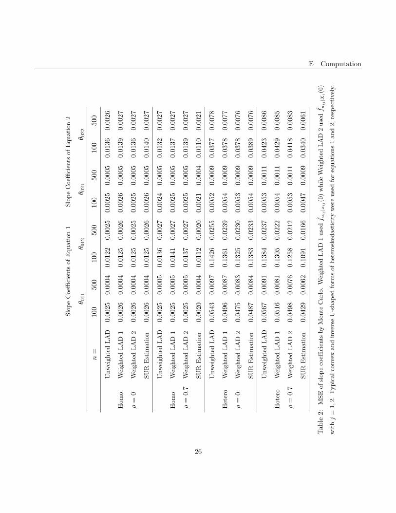
The design of our experiment follows Zhao (2001), i.e.
yij = θ0j0 + xij1θ0j1 + xij2θ0j2 + uij , j = 1, 2,
where θ0j = [θ0j0, θ0j1, θ0j2]′ = [10,−4, 2]′. Like Zhao (2001), we generate the regressors and errors of
equation j by xij1 = Nij + 0.2Uij , xij2 = 0.2Nij + Uij , and uij = hj(Xi)εij , where Nij ∼ N(5, 9),
Uij ∼ U(0, 4), and (εi1, εi2) are jointly normally distributed with mean zero and variance one. In the
10
4 Computation and Simulations
homoskedastic experiments we set h1 = h2 = 1 and the heteroskedastic form used is
h1(Xi) = exp(|x′i1θ01 + x′i2θ02|/10), h2(Xi) = 1 + 3 exp(−(x′i1θ01 + x′i2θ02 + 10)2/100),
where xij = [1, xij1, xij2]′. This is the same design as Zhao (2001) except that we allow the regressors in
one equation to enter the conditional variance function of the other equation. We allow two different values
of the error correlation parameter ρ, namely zero and 0.7. The values for the input parameters used are
βn ∝ n−1/6 and kn ∝ n4/5. The number of replications for each experiment is 1,000 and the results are
summarized in Table 2. For each scenario, we compute regular median regression estimates (Unweighted
LAD), within–equation efficient median estimates (Weighted LAD 1 and 2; a la Zhao (2001)), and our own
estimates (SUR Estimation).
The experiments are designed to investigate the effects of (i) dependence of errors on regressors and
(ii) dependence of errors across equations. In the absence of error correlation with homoskedasticity (top
set of four rows) all estimators have the same limiting distribution, but unweighted LAD does somewhat
better than the others because it does not have the overhead of nonparametric first step estimation. The
effect of such overhead appears, as one would expect, to be less when the number of observations is larger.
With heteroskedasticity, the benefits of the nonparametric correction methods become apparent. Zhao’s
estimator using all regressors (Weighted LAD 2) appears to dominate the competition when there is no
correlation between the errors (third set of rows). It does better than the proposed method because it
has less overhead and beats the other two estimators because of its greater asymptotic efficiency. Our
estimator again narrows the gap when the number of observations increases.
When the errors are correlated, however, the proposed estimator does better than the others. The
degree of such improvement likely depends on the amount of correlation and the sample size. In small
samples with a small amount of error correlation, we recommend Zhao’s procedure using all regressors. If
there is substantial correlation or the data set is sufficiently large then our procedure appears preferable.
11
A Infeasible Estimator
A Infeasible Estimator
Lemma 1 θIp→ θ0.
Proof: Consider the class of functions F ≡c′A1s1(θ) =
∑dj=1 c
′A1js1j(θ) : θ ∈ Θ ⊂ RD
, where
c = [c1, c2, ..., cd]′ is arbitrary and A1j is the jth column vector of A1. Since Gj = 1(y1j ≤ X ′
1jθ) :
θ ∈ Θ ⊂ Rp is a Vapnik Cervonenkis subgraph class (VC class),8 so is Fj ≡ c′A1js1j(θ) : θ ∈ Θ ⊂
Rp.9 Hence F is Euclidean with envelope function E =∑n
j=1 Ej =∑n
j=1 c′A1j (Pakes and Pollard (PP),
1989, lemmas 2.12 and 2.14). Because E(E) < ∞ by A3 and A4, it follows from lemma 2.8 of PP that
supθ∈Θ
∣∣c′mn(θ)− c′m(θ)∣∣ = op(1), and since c is arbitrary, we have supθ∈Θ
∣∣∣∣mn(θ)−m(θ)∣∣∣∣ = op(1). Now,
by the triangle inequality
||m(θI)|| ≤ ||mn(θI)||+ ||m(θ)−mn(θ)|| = op(n−1/2) + op(1) = op(1).
Hence, by assumptions A1, A4 and A5, θI − θ0 = op(1).
Lemma 2 For any positive sequence rn and a consistent estimator θn, mn(θn) = op(rn) implies ||θn −
θ0|| = Op(n−1/2) + op(rn).
Proof: Let δn be a sequence such that P(||θn − θ0|| > δn
)= o(1). Then, since Aisi(θ) is VC,
||m(θn)||triangle≤ ||mn(θn)−m(θn)||+ ||mn(θn)|| . 10 sup
||θ−θ0||<δn
||mn(θ)−m(θ)||+ op(rn)
≤ sup||θ−θ0||<δn
||mn(θ)−m(θ)−mn(θ0) +m(θ0)||+ ||mn(θ0)||+ op(rn)
= op(n−1/2) +Op(n−1/2) + op(rn). (13)
A2, A3 and A4 imply that
m(θ) = Ψ(θ − θ0) + o(||θ − θ0||). (14)
Hence λmin(Ψ)||θn−θ0|| ≤ ||Ψ(θn−θ0)|| ≤ ||m(θn)||+op(||θn−θ0)||, which, together with the consistency of
θn, implies that(λmin(Ψ)− op(1)
)||θn− θ0|| ≤ ||m(θn)|| = Op(n−1/2) + op(rn). Since Ψ is positive definite,
||θn − θ0|| = Op(n−1/2) + op(rn).
8 van der Vaart and Wellner (1996), p.52, problem 14.9 van der Vaart and Wellner (1996), lemma 2.6.18.
10. means that the inequality holds with probability approaching one.
12
B Nonparametric Approximation
Proof of theorem I: Recalling that F is a Euclidean class with envelope function E and noting that
E(E2
)< ∞ and that c is arbitrary, it follows from lemma 2.17 of PP that for any sequence δn with
δn = o(1),
sup||θ−θ0||<δn
∣∣∣∣√n(mn(θ)−m(θ))−√n(mn(θ0)−m(θ0))
∣∣∣∣ = op(1).
Noting that by lemmas 1 and 2, θI − θ0 = Op(n−1/2), using derivations similar to those in (13) and (14)
we have
op(n−1/2) = mn(θI) =(mn(θI)−m(θI)−mn(θ0) +m(θ0)
)+m(θI) +mn(θ0)
= op(n−1/2) + Ψ(θI − θ0) + op(n−1/2) +mn(θ0) = mn(θ0) + Ψ(θI − θ0) + op(n−1/2).
Hence since E(A1s1s′1A
′1) = E(A1T1A
′1) = E(A1F1T
−11 F1A
′1) = V > 0,
√n(θI − θ0) = −V
√nmn(θ0) + op(1) d→ N(0, V ).
B Nonparametric Approximation
In addition to Ti, Ti, Si, Si we define Fj = diag(I(|ujt| ≤ βn)
)/(2βn) and
Ti =n∑
j=1
wijsjs′j , Ti =
n∑j=1
wijTj , Si =n∑
j=1
wijFjX′j , Si =
n∑j=1
wijSj .
Note that
Ai − Ai = (S′i − AiTi)T−1i =
((Si − Si)′ − Ai(Ti − Ti)
)(T−1
i + (T−1i − T−1
i ))
=((Si − Si)′ + (Si − Si)′ − Ai
((Ti − Ti) + (Ti − Ti)
))(T−1
i + (T−1i − T−1
i )). (15)
We deal with the uniform convergence of the differences in turn and then find a bound on Ai.
Lemma 3 ∃ε > 0 : ∀n : P(mini λmin(Ti) < ε
)= 0.
Proof: P(mini λmin(Ti) < ε
)≤ P
(mini λmin(Ti) < ε
)= 0, by A2.
Lemma 4 For any ξni for which E ||ξni||p < ∞ for all i, n and any ε > 0, P (maxi ||ξni|| ≥ ε) ≤
ε−p∑n
i=1 E ||ξni||p.
Proof: We have P (maxi ||ξni|| ≥ ε) ≤∑n
i=1 P (||ξni|| ≥ ε); use the Markov inequality.
13
B Nonparametric Approximation
Lemma 5 For any p > 2 for which E(Rni|Xi) = 0 a.s. and lim supE ||Rni||p <∞,11 maxi ||∑n
j=1wijRnj || =
Op(n1/pk−1/2n ).
Proof: Take ξni = n−1/pk1/2n
∑j wijRj in lemma 4 to obtain
P(max
i
∣∣∣∣∣∣n−1/pk1/2n
n∑j=1
wijRj
∣∣∣∣∣∣ ≥ ε)≤ n−1kp/2
n ε−pn∑
i=1
E∣∣∣∣∣∣ n∑
j=1
wijRj
∣∣∣∣∣∣p = O(1)ε−p,
by lemma L3 of Pinkse (2006). Letting ε→∞ completes the proof.
Lemma 6 For all values of p > 2, maxi ||Ti − Ti|| = Op(k−1/2n n1/p).
Proof: Use lemma 5 with Ri = sis′i − Ti.
We will make frequent use of the inequality
||sj s′j − sjs
′j || ≤ ||sj − sj ||2 + ||sj || · ||sj − sj || ≤ Cs||sj − sj ||, (16)
which holds for some 0 < Cs <∞ since both sj and sj are vectors of zeroes and ones. Let αjr =∣∣∣∣I(|uj | ≤
||Xj ||rι)∣∣∣∣. We will also use the fact that for any sequence rn,
||sj − sj || =∣∣∣∣I(uj ≤ X ′
j(θ − θ0))− I(uj ≤ 0)
∣∣∣∣ ≤ ∣∣∣∣I(|uj | ≤ ||Xj || · ||θ − θ0||ι)∣∣∣∣
≤∣∣∣∣I(|uj | ≤ ||Xj ||rnι
)∣∣∣∣ + I(||θ − θ0|| > rn) = ||αjrn ||+ I(||θ − θ0|| > rn). (17)
Lemma 7 For some C > 0 and any r ≥ 0, E(||αir|| |Xi) ≤ C||Xi||r a.s.
Proof: Note that
0 ≤ E(αirj |Xi) = P (|uij | ≤ r||Xi|| |Xi) = Fuij |Xi(r||Xi||)− Fuij |Xi
(−r||Xi||)A4≤ 2Cf ||Xi||r.
Lemma 8 For any p > 0, maxi ||Ti − Ti|| = Op(ζnpT ).
Proof: First,
C−1s ||Ti − Ti|| = C−1
s
∣∣∣∣∣∣ n∑j=1
wij(sj s′j − sjs
′j)
∣∣∣∣∣∣ (16)
≤n∑
j=1
wij ||sj − sj ||
(17)
≤n∑
j=1
wij
(||αjrn || − E(||αjrn || |Xj)
)+
n∑j=1
wij E(||αjrn || |Xj) + I(||θ − θ0|| > rn). (18)
11 ||Rni|| means the square root of the maximum eigenvalue of R′niRni.
14
B Nonparametric Approximation
Take rn = log n/√n. The third RHS term in (18) is op(κn) for any positive sequence κn since
P[I(||θ − θ0|| > rn) > κn
]= P
[||θ − θ0|| > rn
]= o(1). (19)
For the second RHS term in (18), note that
maxi
n∑j=1
wij E(||αjrn || |Xj)L7≤ Cαrn max
i
n∑j=1
wij ||Xj || ≤ Cαrn maxi||Xi||
L4= Op(rnn1/px) = Op(n1/px−1/2 log n).
Finally, noting that the ||αjrn ||’s are uniformly bounded and independent conditional on the regressors,
Hoeffding’s theorem implies that maxi
∣∣∣∣∣∣∑nj=1wij
(||αjrn ||−E(||αjrn || |Xj)
)∣∣∣∣∣∣ = op(k−1/2n log n), which takes
care of the first RHS term in (18).
Lemma 9 For any p > 0, maxi ||T−1i − T−1
i || = Op(ζnpT ).
Proof: Since T−1i = T−1
i
(I + (Ti − Ti)T−1
i
)−1, the result follows from lemmas 3, 6 and 8.
Lemma 10 maxi ||Si|| = Op(n1/px) and maxi ||Ai|| = Op(n1/px).
Proof: Note that for some 0 < C <∞,
maxi||Ai|| ≤ max
i||Si||max
i||T−1
i ||L3≤ Cmax
i||Si|| ≤ Cmax
i||Si||
A4≤ CCf max
i||Xi||
L4= Op(n1/px).
Lemma 11 maxi ||Si − Si|| = Op
(n1/px(k−1/2
n β1/px−1n + β2
n)).
Proof: Note that
Si − Si =n∑
j=1
wij
(Fj − E(Fj |Xj)
)X ′
j +n∑
j=1
wij
(E(Fj |Xj)− Fj
)X ′
j . (20)
Take Rnj = β1−1/pxn
(Fj − E(Fj |Xj)
)X ′
j in lemma 5 to obtain the rate Op(n1/pxk−1/2n β
1/px−1n ) for the first
RHS term in (20). For the second RHS term note that by the mean value theorem for all t = 1, . . . , d,∣∣∣∣E(Fjt|Xj)− Fjt
∣∣∣∣ =∣∣∣∣6−1β2
nf′′ujt|Xj
(·)∣∣∣∣ A4≤ 6−1Cfβ
2n. (21)
Hence the second RHS term in (20) is bounded by
6−1Cfβ2n max
i
n∑j=1
wij ||Xj || ≤ 6−1Cfβ2n max
i||Xi|| = Op(n1/pxβ2
n).
15
B Nonparametric Approximation
Lemma 12 maxi ||Si − Si|| = Op(n1/2k−1n β−1
n log n).
Proof: Let rn = log n/√n. Now,
maxi||Si − Si|| = max
i||Si − Si||I(||θ − θ0|| ≤ rn) + max
i||Si − Si||I(||θ − θ0|| > rn). (22)
By (19), the second RHS term in (22) is negligble. For the first RHS term in (22) using the inequality (for
generic a, b, t)∣∣I(|a| ≤ t)− I(|b| ≤ t)
∣∣ ≤ I(|b| ≤ t+ |a− b|)− I(|b| ≤ t− |a− b|), it follows that
2βn||Fj − Fj ||I(||θ − θ0|| ≤ rn) ≤∣∣∣∣∣∣I(|uj | ≤ (βn + ||Xj ||rn)ι
)− I
(|uj | ≤ (βn − rn||Xj ||)ι
)∣∣∣∣∣∣, (23)
and hence
2 maxi||Si − Si||I(||θ − θ0|| ≤ rn) ≤ 2 max
i
n∑j=1
wij ||Xj || · ||Fj − Fj ||
≤ β−1n max
i
n∑j=1
wij ||Xj ||∣∣∣∣∣∣I(|uj | ≤ (βn + ||Xj ||rn)ι
)− I
(|uj | ≤ (βn − rn||Xj ||)ι
)∣∣∣∣∣∣A6≤ Cw(knβn)−1
n∑j=1
||Xj ||∣∣∣∣∣∣I(|uj | ≤ (βn + rn||Xj ||)ι
)− I
(|uj | ≤ (βn − rn||Xj ||)ι
)∣∣∣∣∣∣. (24)
Since for all t = 1, . . . , d,
E(I(|ujt| ≤ (βn+rn||Xj ||)
)−I
(|ujt| ≤ (βn−rn||Xj ||)
)|Xj
)= Fujt|Xj
(βn+rn||Xj ||)−Fujt|Xj(βn−rn||Xj ||)
= fujt|Xj(·)||Xj ||rn ≤ Cfrn||Xj ||, (25)
the unconditional expectation of (24) is bounded by
dCwCfrn(knβn)−1n∑
j=1
E||Xj ||2 = O(nrn(knβn)−1
)= O(n1/2k−1
n β−1n log n).
Lemma 13 maxi ||Ai − Ai|| = op(1).
Proof: Using lemmas 3, 6, 8, 9, 10, 11 and 12 in (15) yields
Ai − Ai = Op
((n1/pxζnpT + ζnpS)(1 + ζnpT ) A7= op(1).
16
B Nonparametric Approximation
Observe that
√n(mn(θ0)−mn(θ0)
)= n−1/2
n∑i=1
(Ai −Ai)si = n−1/2n∑
i=1
(Ai − Ai)si + n−1/2n∑
i=1
(Ai −Ai)si. (26)
We use the expansion in (15) to deal with the first RHS term and show the following results.
n−1/2n∑
i=1
Ai(Ti − Ti)T−1i si = op(1), (27)
n−1/2n∑
i=1
Ai(Ti − Ti)T−1i si = op(1), (28)
n−1/2n∑
i=1
(Si − Si)′T−1i si = op(1), (29)
n−1/2n∑
i=1
(Si − Si)′T−1i si = op(1), (30)
n−1/2n∑
i=1
Ai(Ti − Ti)(T−1i − T−1
i ) = op(1), (31)
n−1/2n∑
i=1
(Si − Si)′(T−1i − T−1
i ) = op(1), (32)
n−1/2n∑
i=1
(Ai −Ai)si = op(1). (33)
Condition (27) is dealt with in lemmas 14–16, (28) in lemmas 17–18, (29) and (30) in lemmas 19–20,
(31) and (32) in lemmas 21–22 and 33 in lemmas 23–25.
Lemma 14 Let ξi be a sequence of random variables for which E(ξi|X, ξi−1, . . . , ξ1) = 0 and for which
ess sup(||ξi||) ≤ 1. Then maxj ||∑n
i=1wijξi|| = op(√n log n/kn).
Proof: Let εn = Cw(√
3n log n+ 2)/kn. Then
P(max
j
∣∣∣∣∣∣∑i
wijξi
∣∣∣∣∣∣ ≥ 2εn)≤ P
(max
j
∣∣∣∣∣∣ n∑i6=j
wijξi
∣∣∣∣∣∣ ≥ εn
)+ P
(max
jwjj ||ξj || ≥ εn
)Bonferroni
≤n∑
j=1
P(∣∣∣∣∣∣ n∑
i6=j
wijξi
∣∣∣∣∣∣ ≥ εn
)+ I(Cw/kn ≥ εn) =
n∑j=1
EP(∣∣∣∣∣∣ n∑
i6=j
wijξi
∣∣∣∣∣∣ ≥ εn|X),
where we used the fact that maxj wjj ||ξj || ≤ Cw/kn with probability one. We then used the law of iterated
expectations and the fact that I(εn ≤ Cw/kn) = 0. Since ξi = wijξi forms a martingale difference sequence
for each j conditional on X and ||ξi|| ≤ wij a.s., we apply Azuma’s inequality (e.g. Davidson (1994, p245))
to the RHS to obtain an upper bound of
2n exp(− ε2n
2∑
iw2ij
)≤ 2n exp
(−3C2
wnk−2n log n
2nC2wk
−2n
)= 2n−1/2 = o(1).
17
B Nonparametric Approximation
Lemma 15 Let ξi be as in lemma 14 and let ξni = Ξni(X)ξi, where for some pΞ > 0, lim supE ||Ξni(X)||pΞ <
∞. Then maxj
∣∣∣∣∣∣∑ni=1wijξni
∣∣∣∣∣∣ = op
(n1/pΞ+1/2k−1
n log n).
Proof: Let ε∗n = n1/pΞ√
log n, εn =√
3Cwn1/pΞ+1/2 log n/kn and ξ∗ni = ξniI
(||Ξni(X)|| ≤ ε∗n
)/ε∗n. Then
P(max
j
∣∣∣∣∣∣ n∑i=1
wijξni
∣∣∣∣∣∣ ≥ 2εn)
= P(max
j
∣∣∣∣∣∣ n∑i=1
wij
(ε∗nξ
∗ni + ξniI(||Ξni(X)|| > ε∗n)
)∣∣∣∣∣∣ ≥ 2εn)
≤ P(max
j
∣∣∣∣∣∣ n∑i=1
wijξ∗ni
∣∣∣∣∣∣ ≥ 2εnε∗n
)+ P
(max
i||Ξni(X)|| ≥ ε∗n
). (34)
The second RHS term in (34) is by lemma 4 bounded by (ε∗n)−pΞ∑n
i=1 E ||Ξni||pΞ = O((log n)−pΞ/2
)= o(1).
The first RHS term in (34) is also o(1) because ess sup ||ξ∗ni|| ≤ 1 by construction and lemma 14 can be
applied since
εnε∗n
=√
3CwnpΞ+2
2pΞ log n/kn
n1/pΞ√
log n=Cw√
3n log nkn
.
Lemma 16 n−1/2∑
i Ai(Ti − Ti)T−1i si = op(1).
Proof: The LHS is∣∣∣∣∣∣n−1/2n∑
j=1
n∑i=1
wijAi(sj s′j − sjs
′j)T
−1i si
∣∣∣∣∣∣ L15≤
n∑j=1
||sj s′j − sjs
′j || × op(n1/pxk−1
n log n)
(16)
≤ Cs
n∑j=1
||sj − sj || × op(n1/pxk−1n log n). (35)
Set rn = log n/√n. Now,
n∑j=1
||sj − sj ||(17)
≤n∑
j=1
(||αjrn || − E(||αjrn || |X)
)+
n∑j=1
E(||αjrn || |X) + nI(||θ − θ0|| > rn). (36)
The third RHS term is op(1) by (19) and the second RHS term is by lemma 7 bounded by Cαrn∑n
j=1 ||Xj || =
Op(nrn) = Op(n1/2 log n). Squaring the first RHS term and taking its expectation yields
n∑j=1
E(||αjrn || − E(||αjrn || |X)
)2 L7≤ Cnrn = O(nrn).
Hence the RHS in (36) is Op(√nrn) +Op(
√n log n) +Op(1) = Op(
√n log n), which implies that the RHS
in (35) is op
(n1/px+1/2k−1
n (log n)2)
= op(1) by A7.
18
B Nonparametric Approximation
Lemma 17 Let ξnij = ξn(ui, uj ;X) be such that E(ξnij |ui, X) = E(ξnij |uj , X) = 0 a.s. for all i, j and
maxi,j E ||ξnij ||2 = O(1). Then n−1∑n
i,j=1wijξnij = Op(k−1n ).
Proof: Square the LHS and take the expectation to obtain
n−2n∑
i,j=1
(E(w2
ij ||ξnij ||2) + E(wijwjiξ′nijξnji)
) A6≤ 2C2
wk−2n max
i,jE ||ξnij ||2 = O(k−2
n ).
Lemma 18 n−1/2∑n
i=1 Ai(Ti − Ti)T−1i si = op(1).
Proof: In lemma 17, take ξnij = Ai(sjs′j−Tj)T−1
i si to obtain a convergence rate of Op(n1/2k−1n ) = op(1).
Lemma 19 n−1/2∑
i(Si − Si)′T−1i si = op(1).
Proof: The norm of the LHS is∣∣∣∣∣∣n−1/2n∑
j=1
(Fj − Fj)X ′j
n∑i=1
wijT−1i si
∣∣∣∣∣∣ ≤ maxj
∣∣∣∣∣∣n−1/2n∑
i=1
wijT−1i si
∣∣∣∣∣∣ n∑j=1
||Fj − Fj || × ||Xj ||
L14= Op(k−1n
√log n)
n∑j=1
||Fj − Fj || × ||Xj ||.
Let (as in lemma 12) rn = log n/√n. Then
n∑j=1
||Fj − Fj || × ||Xj || =n∑
j=1
||Fj − Fj || × ||Xj ||I(||θ− θ0|| ≤ rn) +n∑
j=1
||Fj − Fj || × ||Xj ||I(||θ− θ0|| > rn)
(19)=
n∑j=1
||Fj − Fj || × ||Xj ||I(||θ − θ0|| ≤ rn) + op(1).
Finally,√
log nkn
n∑j=1
||Fj−Fj ||×||Xj ||I(||θ−θ0|| ≤ rn)(23),(25)
≤Cfdrn
√log n
knβn
n∑j=1
||Xj ||2 = Op
(√n(log n)2
knβn
)A7= op(1).
Lemma 20 n−1/2∑n
i=1(Si − Si)′T−1i si = op(1).
Proof: The LHS is
n−1/2n∑
i,j=1
wij
(Fj − E(Fj |Xj)
)X ′
jT−1i si + n−1/2
n∑i,j=1
wij
(E(Fj |Xj)− Fj
)X ′
jT−1i si. (37)
19
B Nonparametric Approximation
The first RHS term is Op(n1/2β−1/2n k−1
n ) = op(1) by lemma 17. The norm of the second RHS term is
bounded by
n−1/2 maxj
∣∣∣∣∣∣ n∑i=1
wijT−1i si
∣∣∣∣∣∣ n∑j=1
wij
∣∣∣∣E(Fj |Xj)− Fj
)∣∣∣∣× ||Xj ||
L14,(21)
≤ Op(k−1n
√log n)6−1Cfβ
2n
∑j
||Xj || = Op(nk−1n β2
n
√log n) A7= op(1).
Lemma 21 n−1/2∑n
i=1 Ai(Ti − Ti)(T−1i − T−1
i )si = op(1).
Proof: Note that by lemmas 8, 9 and assumption A7,
∣∣∣∣∣∣n−1/2n∑
i=1
Ai(Ti − Ti)(T−1i − T−1
i )si
∣∣∣∣∣∣≤ max
i
∣∣∣∣Ti − Ti
∣∣∣∣× ∣∣∣∣T−1i − T−1
i
∣∣∣∣× n−1/2n∑
i=1
||Ai|| × ||si|| = Op(√nζ2
npT ) = op(1).
Lemma 22 n−1/2∑n
i=1(Si − Si)′(T−1i − T−1
i )si = op(1).
Proof: Use a similar inequality to the one used in lemma 21 to obtain a rate of n1/2ζnpSζnpT = o(1) by
A7.
Lemma 23 E ||Ai −Ai||2 = o(1).
Proof: The square of the LHS is bounded by C(E ||Ai||4 E ||Ti − Ti||4 + (E ||Si − Si||2)2
)= o(1), by
theorem 1 of Stone (1977).
Lemma 24 n−1/2∑n
i=1(Ai −Ai)si = op(1).
Proof: E∣∣∣∣∣∣n−1/2
∑ni=1(Ai −Ai)si
∣∣∣∣∣∣2 ≤ E ||Ai −Ai||2 = o(1), by lemma 23.
Lemma 25 mn(θ0)−mn(θ0) = op(n−1/2).
Proof: Using the expansion in (26) and (27)–(33), the stated result follows from lemmas 16, 18, 19, 20,
21, 22, and 24.
20
C Feasible Estimator
C Feasible Estimator
Lemma 26 There exists a positive sequence µ1n with µ1n = o(1) such that for any positive sequence
rn, n−1∑n
i=1 ||Ai −Ai|| ||αirn || = op(rnµ1n).
Proof: Let µ1n be such that µ1n = o(1) and E ||Ai − Ai||2 = o(µ21n); such µ1n exist by lemma 23. Now,
E(||Ai −Ai|| ||αirn ||
) L7≤ Crn E
(||Ai −Ai|| ||Xi||
) Schwarz≤ Crn
√E
(||Ai −Ai||2
)√E ||Xi||2 = o(rnµ1n).
Let Θr = θ ∈ Θ : ||θ − θ0|| < r.
Lemma 27 There exists a positive sequence µn with µn = o(1) such that for any positive sequence rn,
supθ∈Θrn||mn(θ)−mn(θ)|| = op(rnµn + n−1/2).
Proof: First note that
supθ∈Θrn
||mn(θ)−mn(θ)||triangle≤ sup
θ∈Θrn
||mn(θ)−mn(θ)− mn(θ0) +mn(θ0)||+ ||mn(θ0)−mn(θ0)||
L25≤ sup
θ∈Θrn
n−1n∑
i=1
||Ai −Ai|| ||si(θ)− si(θ0)||+ op(n−1/2) ≤ n−1n∑
i=1
||Ai −Ai|| ||αirn ||+ op(n−1/2).
Now, let µ1n be as in lemma 26 and µ2n be such that maxi ||Ai −Ai|| = op(µ2n) and µ2n = o(1); such µ2n
exist by lemma 13. Then by the triangle inequality,
n−1n∑
i=1
||Ai −Ai|| ||αirn || ≤ n−1n∑
i=1
||Ai − Ai|| ||αirn ||+ n−1n∑
i=1
||Ai −Ai|| ||αirn ||
≤ maxi||Ai−Ai||n−1
n∑i=1
||αirn ||+n−1n∑
i=1
||Ai−Ai|| ||αirn ||L7,L13,L26
= op(µ2n)Op(rn)+op(µ1nrn) = op
((µ1n+µ2n)rn
),
Take µn = µ1n + µ2n.
Lemma 28 mn(ˆθ) = op(n−1/2).
Proof: Let ψn be such that || ˆθ − θ0|| = Op(ψn) but || ˆθ − θ0|| 6= op(ψn). Let µn be as in lemma 27.
Then for rn = ψn/√µn we have
||mn(ˆθ)||triangle≤ ||mn(ˆθ)−mn(ˆθ)||+||mn(ˆθ)|| . sup
θ∈Θrn
||mn(θ)−mn(θ)||+op(n−1/2) L27= op(ψn√µn)+op(n−1/2).
So by lemma 2, || ˆθ − θ0|| = op(ψn) +Op(n−1/2). Hence ψn ∼ n−1/2.
21
E Computation
Proof of theorem II: By lemma 28, ˆθ satisfies (8).
D Covariance Matrix Estimation
Proof of theorem III: Let Ψ = n−1∑n
i=1 AiSi. Then
Ψ− Ψ = n−1n∑
i=1
(Ai − Ai)(Si − Si) + n−1n∑
i=1
(Ai − Ai)Si + n−1n∑
i=1
Ai(Si − Si),
such that Ψ− Ψ = op(1) by lemmas 11, 12 and 13. To show Ψ−Ψ = op(1), which is sufficient since Ψ > 0
by assumption, we can use an expansion similar to the one above, which leads to
E ||Ψ−Ψ|| = E∣∣∣∣∣∣n−1
n∑i=1
(AiSi −AiSi)∣∣∣∣∣∣
≤ E(||Ai −Ai|| × ||Si − Si||
)+ E
(||Ai|| × ||Si − Si||
)+ E
(||Ai −Ai|| × ||Si||
)Schwarz≤
√E ||Ai −Ai||2
√E ||Si − Si||2 +
√E ||Ai||2
√E ||Si − Si||2 +
√E ||Ai −Ai||2
√E ||Si||2.
Apply lemma 23, theorem 1 of Stone (1977) and the fact that E ||Ai||2,E ||Si||2 <∞ by assumption.
E Computation
Proof of theorem IV: By lemma 27 and theorem III it follows that θ(1) = Op(n−1/2). Hence by lemma
2, mn(θ(j))−mn(θ(j)) = op(n−1/2) for j = 0, 1. Because Aisi is a VC class (see (13)), it follows that
∣∣∣∣mn(θ(1))−mn(θ(0))−m(θ(1)) +m(θ(0))∣∣∣∣ = op(n−1/2).
Since m(θ(1))−m(θ(0)) = Ψ(θ(1) − θ(0)) + op(n−1/2) (see (14)), it follows that
mn(θ(1))− mn(θ(0)) = mn(θ(1))−mn(θ(0)) + op(n−1/2) = m(θ(1))−m(θ(0)) + op(n−1/2)
= Ψ(θ(1) − θ(0)) + op(n−1/2) = −V −1V (θ(0))mn(θ(0)) + op(n−1/2) Th.III= −mn(θ(0)) + op(n−1/2).
So mn(θ(1)) = op(n−1/2) and (9) is satisfied.
22
E Computation
References
Aitken, A. C. (1935) On least squares and linear combination of observations. Proceedings of the Royal
Society of Edinburgh 55, 42–48.
Carroll, R. J. (1982) Adapting for heteroscedasticity in linear models. Annals of Statistics 10, 1224–1233.
Chamberlain, G. (1987) Asymptotic efficiency in estimation with conditional moment restrictions. Journal
of Econometrics 34, 305–334.
Davidson, J. (1994) Stochastic limit theory. New York: Oxford University Press.
Delgado, M. (1992) Semiparametric generalized least squares estimation in the multivariate nonlinear
regression model. Econometric Theory 8, 203–222.
Koenker, R. (2005) Quantile regression. New York: Cambridge University Press.
Koenker, R. & Q. Zhao (1994) L–estimation for linear heteroscedastic models. Journal of Nonparametric
Statistics 3, 223–235.
Komunjer, I. & Q. Vuong (2006) Efficient Conditional Quantile Estimation: The Time Series Case. UCSD
working paper.
Newey, W. K. (1990) Efficient instrumental variables estimation of nonlinear models. Econometrica 58,
809–837.
Newey, W. K. (1993), Efficient estimation of models with conditional moment restrictions. In G.S. Mad-
dala, C.R. Rao and H.D. Vinod (ed.) Handbook of Statistics 11. Amsterdam: North Holland, pp 419–454.
Newey, W. K. & J. L. Powell (1990) Efficient estimation of linear and type I censored regression models
under conditional quantile restrictions. Econometric Theory 6, 295–317.
Pakes, A. & D. Pollard (1989) Simulation and the asymptotics of optimization estimators. Econometrica
23
E Computation
57, 1027–1057.
Pinkse, J. (2006) Heteroskedasticity correction and dimension reduction. Pennsylvania State University
working paper.
Robinson, P. M. (1987) Asymptotically efficient estimation in the presence of heteroskedasticity of un-
known form. Econometrica 55, 875–891.
Stone, C. J. (1977) Consistent nonparametric regression. Annals of Statistics 5, 595–645.
van der Vaart, A. & J. A. Wellner (1996) Weak convergence and empirical processes: with applications to
statistics. New York: Springer.
Whang, Y. (2006) Smoothed Empirical Likelihood Methods for Quantile Regression Models. Econometric
Theory 22, 173–205.
Zhao, Q. (2001) Asymptotically efficient median regression in the presence of heteroskedasticity of un-
known form. Econometric Theory 17, 765–784.
24
E Computation
No Overlap Overlap in θ01, θ02
xi1 = xi2 xi1 6= xi2 xi1 = xi2 xi1 6= xi2
xi1, xi2 ⊥⊥ ui1, ui2 ui1 ⊥⊥ ui2 all same all same J<S∗,S,O J<S∗,S,O
ui1 6⊥⊥ ui2 all same J<S∗,S,O J<S∗,S,O J<S∗,S,O
xij ⊥⊥ uij∗ ; j 6= j∗ ui1 ⊥⊥ ui2|xi1, xi2 all same J,S∗,S<O J<S∗,S,O J<S∗,S<O
ui1 6⊥⊥ ui2|xi1, xi2 all same J<S∗,S<O J<S∗,S,O J<S∗,S<O
xij 6⊥⊥ uij∗ ui1 ⊥⊥ ui2|xi1, xi2 J,S∗,S<O J,S∗<S<O J<S∗,S<O J<S∗<S<O
ui1 6⊥⊥ ui2|xi1, xi2 J<S∗,S<O J<S∗<S<O J<S∗,S<O J<S∗<S<O
The entries indicate which methods are preferable to others in terms of asymptotic efficiency in various situations.
‘⊥⊥’ denotes independence and ‘<’ means “is typically more efficient but never less efficient than.” J=joint estimation
(new methodology), S=separate estimation (Zhao’s method), S∗=separate estimation using the regressors from both
equations (Zhao’s results can be used for this) and O=no efficiency correction.
Please note: when errors are independent of each other and of the regressors and there are no cross–equation
restrictions on the coefficient vectors, then equation by equation adaptive (to error distribution) estimation dominates
all of the other estimation methods mentioned here.
This comparison applies equally to mean and quantile regressions.
Table 1: Asymptotic Efficiency Comparison of Semiparametric Methods
25
E ComputationSl
ope
Coe
ffici
ents
ofE
quat
ion
1Sl
ope
Coe
ffici
ents
ofE
quat
ion
2
θ 011
θ 012
θ 021
θ 022
n=
100
500
100
500
100
500
100
500
Unw
eigh
ted
LA
D0.
0025
0.00
040.
0122
0.00
250.
0025
0.00
050.
0136
0.00
26
Hom
oW
eigh
ted
LA
D1
0.00
260.
0004
0.01
250.
0026
0.00
260.
0005
0.01
390.
0027
ρ=
0W
eigh
ted
LA
D2
0.00
260.
0004
0.01
250.
0025
0.00
250.
0005
0.01
360.
0027
SUR
Est
imat
ion
0.00
260.
0004
0.01
250.
0026
0.00
260.
0005
0.01
400.
0027
Unw
eigh
ted
LA
D0.
0025
0.00
050.
0136
0.00
270.
0024
0.00
050.
0132
0.00
27
Hom
oW
eigh
ted
LA
D1
0.00
250.
0005
0.01
410.
0027
0.00
250.
0005
0.01
370.
0027
ρ=
0.7
Wei
ghte
dLA
D2
0.00
250.
0005
0.01
370.
0027
0.00
250.
0005
0.01
390.
0027
SUR
Est
imat
ion
0.00
200.
0004
0.01
120.
0020
0.00
210.
0004
0.01
100.
0021
Unw
eigh
ted
LA
D0.
0543
0.00
970.
1426
0.02
550.
0052
0.00
090.
0377
0.00
78
Het
ero
Wei
ghte
dLA
D1
0.04
960.
0087
0.13
610.
0239
0.00
540.
0009
0.03
780.
0077
ρ=
0W
eigh
ted
LA
D2
0.04
750.
0083
0.13
250.
0230
0.00
530.
0009
0.03
780.
0076
SUR
Est
imat
ion
0.04
870.
0084
0.13
830.
0233
0.00
540.
0009
0.03
890.
0076
Unw
eigh
ted
LA
D0.
0567
0.00
910.
1384
0.02
370.
0053
0.00
110.
0423
0.00
86
Hot
ero
Wei
ghte
dLA
D1
0.05
160.
0081
0.13
050.
0222
0.00
540.
0011
0.04
290.
0085
ρ=
0.7
Wei
ghte
dLA
D2
0.04
980.
0076
0.12
580.
0212
0.00
530.
0011
0.04
180.
0083
SUR
Est
imat
ion
0.04
290.
0062
0.10
910.
0166
0.00
470.
0009
0.03
400.
0061
Tab
le2:
MSE
ofsl
ope
coeffi
cien
tsby
Mon
teC
arlo
.W
eigh
ted
LA
D1
usedf u
ij|x
ij(0
)w
hile
Wei
ghte
dLA
D2
usedf u
ij|X
i(0
)
wit
hj
=1,
2.T
ypic
alco
nvex
and
inve
rse
U-s
hape
dfo
rms
ofhe
tero
sked
asti
city
wer
eus
edfo
req
uati
ons
1an
d2,
resp
ecti
vely
.
26