Efficient parallel algorithms and VLSI architectures for manipulator Jacobian computation

1154 IEEE TRANSACTIONS ON SYSTEMS, MAN, AND CYBERNETICS. VOL. 19, NO. 5. SEPTEMBER/OCTOBER 1989

Efficient Parallel Algorithms and VLSI Archtectures for Manipulator

Jacobian Computation

Abstract --The real-time computation of manipulator Jacobian that relates the manipulator joint velocities to the linear and angular velocities of the manipulator end-effector is pursued. Since the Jacobian can be expressed in the form of the first-order linear recurrence, the time lower bound to compute the Jacobian can be proved to be of order O ( N ) on uniprocessor computers, and of order O(log, N ) on both parallel single-in- shuction-stream multiple-data-stream (SIMD) computers and parallel VLSI pipelines, where N is the number of l inks of the manipulator. To achieve the computation time lower bound, we developed the generalized- k method on uniprocessor computers, the parallel forward and backward recursive doubling algorithm (PFABRD) on SIMD computers, and a parallel systolic architecture on VLSI pipelines. All the methods are capable of computing the Jacobian at any desired reference coordinate frame k from the base coordinate frame to the end-effector coordinate frame. The computation effort in terms of floating point operations is minimal when k is in the range (4, N - 3) for the generalized- k method, and k = ( N + 1 ) / 2 for both the PFABRD algorithm and the parallel pipeline.

I. INTRODUCTION

HE CONTROL of robot manipulators involves actu- T ating appropriate joint motors to position and orient the manipulator end-effector along a planned trajectory. For some applications such as paint spraying and seam welding, it is desirable to command the manipulator end- effector to move in a desired Cartesian direction in a coordinated rate control. The motions of various joint motors are combined and resolved into separately control- lable hand motions along the world coordinate system. This implies that several joint motors must run simultaneously at different time-varying rates in order to acheve the desired coordinated hand rate motion along any world coordinate axis. This resolved motion control concept requires one to determine how each infinitesimal joint motion affects the infinitesimal motion of the manipulator end-effector. An advantage of resolved motion is that there

Manuscript received June 1, 1987: revised March 12, 1989. This work was supported in part by the National Science Foundation under Grant CDR 8803017 to the Engineering Research Center for Intelligent Manu- facturing Systems. This work was partially presented at the 1988 IEEE Int. Conf. on Robotics and Automation, Philadelphia, PA, Apr. 24-29, 1988.

T. B. Yueng was with the School of Electrical Engineering, Purdue University. He is now with LSI Logic Corp, 1501 McCarthy Blvd., MS-E 192, Milpitas, CA 95035.

C. S. G. Lee is with the School of Electrical Engineering, Purdue University, West Lafayette, IN 47907.

IEEE Log Number 8929127.

exists a linear mapping between the infinitesimal joint motion space and the infinitesimal hand motion space. This mapping is defined by the manipulator Jacobian.

In robotics the position and orientation (i.e., pose), x, of the end-effector of an N-link manipulator relative to a fixed inertial coordinate system can be described by

x = f ( 4 ) (1) where q is an N-dimensional joint-variable vector for the N-link manipulator. Differentiating (1) with respect to time yields

i ( t ) e [ 4 1 = J ( q ) q ( t ) 6x1

where U and o are, respectively, the linear and angular velocities of the manipulator end-effector, q e ( ql, q2, . . . , qN)T is the joint-velocity vector of the manipulator,

and the superscript T indicates matrix/vector transpose. J(q ) is the 6 X N manipulator Jacobian matrix and it is a function of joint variables. In essence the manipulator Jacobian specifies the mapping from the joint velocities in the joint-variable space to the linear and angular velocities in the Cartesian space. In addition the transpose of the Jacobian matrix relates static contact forces and moments to a set of joint torques as

7 = J T ( q ) F (3) where F L! (F,, F,, F,, M,, M,, M z ) T is a 6-dimensional static force/moment vector, -and 7 is an N-dimensional joint-torque vector. Consequently the study of the Jaco- bian computation is an important aspect in robotic lune- matics and control. This paper focuses on the real-time computation of manipulator Jacobian in uniprocessor computers, parallel computers, and VLSI pipelines.

Existing methods in computing the Jacobian are confined to uniprocessor computers. In particular Renaud [13], Waldron [16], and Orin/Schrader [lo] exploited the linear recurrence characteristics of the Jacobian equations. Their methods differed from each other only by a different selection of the reference coordinate frame for computation. The reference coordinate frame is selected such that all the vectors and the Jacobian computed are referred to that reference coordinate system. Specifically for an N-link

0018-9472/89/0900-ll54$01.00 01989 IEEE

YEUNG AND LEE: ALGORITHMS AND VLSI ARCHITECTURES FOR MANIPULATOR JACOBIAN COMPUTATION 1155

TABLE I COMPARISON OF VARIOUS METHODS FOR THE JACOBIAN COMPUTATION

Reference Coordinate Addi tiom/ No. of Methods Frame k Multiplications Subtractions Processors

Vukobratovic/Potkonjak“ N Paul et al.“ N Fu et ul. 0 Waldron’ 0 Orin and Schraderh N Renaud’ N/2 Generalized-k ’.‘ Q g k d N

PFABRD‘ O d k d N (optimal k E [4, N - 31)

(optimal k = I( N + 1)/21)

“Order quoted from the reference [lo]. ’Twist angle a, is set to *90 degrees. ‘The optimal k case is quoted.

robot manipulator, Waldron’s method corresponds to the reference coordinate frame k being selected at the base coordinates k = 0, Renaud’s method corresponds to k =

N/2, and Orin/Schrader’s method corresponds to selecting the reference coordinate frame at the end-effector coordinates k = N . They all have a computational order of O ( N ) for an N-link manipulator.

Other methods for computing the Jacobian include Uicker [14], Groome [3], Whitney [17], Paul et al. [12], Vukobratovic and Potkonjak [15], and Fu et al. [2]. Uicker [14] obtained the Jacobian in terms of the differential change of transform elements. Groome [3] and Whitney [17] computed the Jacobian based on vector methods. Paul et al. [12] developed the differential matrix approach to obtain the Jacobian directly from the homogeneous transformation matrices. Vukobratovic and Potkonjak [15] calculated the N individual columns of the Jacobian matrix from the base coordinates to the end-effector coordinates expressed with respect to the end-effector coordinates. In Fu et al. [2], the Jacobian is computed as a by-product from the computation of the Newton-Euler equations of motion in solving the robot inverse dynamics.

Recently Orin et al. [ll] developed pipeline and parallel algorithms for configuring a systolic array of processors to implement the Jacobian. ( N + 1)/2 time units are taken to obtain the Jacobian for the pipeline algorithm, and 2 N processors are used with an initiation rate equal to 2. The parallel algorithm, which is based on a “divide and con- quer” strategy, reduces the computational order to O(log, ( N + 1)). Hypercube interconnection network is selected for connecting the processors.

Based on the linear recurrence property, this paper presents the development of the generalized-k algorithm which computes the Jacobian on uniprocessor computers in the order of O ( N ) at any given desired reference coordinate frame ( k ) . Waldron’s, Renaud’s, and Orin/ Schrader’s methods are special cases of the generalized-k algorithm. We also find from the generalized-k algorithm that the coefficient and the order are fixed with respect to any k ; however the total number of computations is minimum if k is in the range of (4, N -3) for an N-link manipulator. In order to overcome the recurrence problem

10N2 - 15N + 9 N 2 + 72N - 2 1 30N - 18 14N - 15 1

30N - 31 18N - 24 1 30N - 74 18N - 51 1

30N - 105 18N - 75 1

12N2 1 1 2 N (19/2)( N 2 + N ) 1

30N - 105 18N - 75 1

in the Jacobian, a parallel forward and backward recursive doubling (PFABRD) algorithm running on single-instruction-stream multiple-data-stream (SIMD) computers is developed to yield the time lower bound of O(log,N). To further reduce the speed of computation, a linear VLSI systolic pipeline is designed to implement the generalized-k algorithm, and a parallel VLSI systolic pipeline is designed to implement the PFABRD algorithm. The linear pipe takes 18 modular processors and 3N floating-point operations (flops) to complete the task, whereas the parallel pipe takes (18N - 36) modular processors and (4m + 5) flops, where

N + 1

2 IL .

Existing methods and the proposed methods for the computation of the Jacobian are tabulated in Tables I and I1 for comparison.

11. NOTATION AND JACOBIAN EQUATIONS

To describe the translational and rotational relationship between adjacent links, a Denavit-Hartenberg matrix rep- resentation [l] for each link is used. An orthonormal coordinate frame system (x,, y,,z,) is assigned to link i, where the z , axis passes through the axis of motion of joint ( i + 1). With t h s orthonormal coordinate frame, four parameters are used to characterize two successive coordinate systems: a, is the common normal distance between the z , - ~ and z, axes; a, is the twist angle measured between the z , ~ ~ and z , axes in a plane perpendicular to a,; d, is a distance parameter measured between the x l p 1 and x, axes; 8, is a joint angle between the normals and measured in a plane normal to the joint axis. Once the link coordinate systems have been established for each link, a homogeneous transformation matrix, ‘-9 ,, can easily be developed to relate the ith coordinate frame to the ( i - 1)th

1156 IEEE TRANSACTIONS ON SYSTEMS, MAN, AND CYBERNETICS, VOL. 19, NO. 5, SEPTEMBER/OCTOBER 1989

TABLE I1 COMPARISON OF VLSI ARCHITECTURES FOR THE JACOBIAN COMPUTATION

Reference Coordinate No. of Computation Initial Time-Processor Methods Frame k Processors Time Delay Product

Orin et U / . [ l l ] N O(N) O(N) 00) 0 ( N 2 ) linear pipe

parallel pipe

linear pipe

parallel pipe

Orin et U / . [ I l l N O(N) O(log2 ( N + 1)) O ( k 2 ( N + 1)) O(Nlog, N )

Yeung and Lee O b k G N O(1) O(N) O(1) O ( N )

Yeung and Lee" O b k g N O(N) O ( k 2 ( N - 11/21 O ( h * ( N - 11/21 O(Nlog2 N )

"The optimal k case is quoted.

coordinate frame [2]

sin a, sin e, I a, cos e, , - 'A , = [ sin 8, cos a, cos e, - sin a, cos e, j a, sin e, ' I cos e, - cos a, sin e,

0 sin a, cosa, I d, _-_----------------_--------------

0 0 0 I 1

where ' - 'Ri is the rotation matrix relating the orientation

0

of link i coordinate frame with respect to link i - 1 coordinate frame, and '-'q is the position vector from the origin of link i - 1 to the origin of link i. In order to derive the Jacobian equations, we will consistently use the coordinate

0

Fig. 1. Coordinate system and its parameters

frame. From Fig. 1 system shown in Fig. 1. The parameters are defined in the following.

01

z i

Ai

Jk

kw;

kn;

k P i

kSi

'pi

is the origin of the i th coordinate frame. is the unit vector along the z axis of the ith coordinate frame with reference to the inertial coordinate frame. is the joint indicator indicating whether joint i is prismatic ( A , = 1) or revolute ( A , = 0). is the Jacobian matrix with elements referenced to the k th coordinate frame. is the angular velocity of link i in the Cartesian space expressed in the k th reference coordinate frame. is the linear velocity of link i in the Cartesian space expressed in the k th reference coordinate frame. is an entry of Jk relating 4; to 'vu, as

k k v, = pLiqi, where k p i =

is an entry of Jk relating qi to "ai as - -

'a, =ki3,41, where 'bj =

is the position vector from the origin of link k to the origin of link i in the k th reference coordinate

s

for i > k , (sa) k k

k k p , = p l + l + k R , + l l + l p : + l ,

PI = Pl- l -kR;P:> for i < k . (8b)

In particular, 'p: is the position vector from the origin of link i

coordinate f r p e to the origin of link i - 1 coordinate frame with respect to the link i coordinate frame; it can be shown that

- a, - d, sina, . [ - d,cosa,]

(9) I p : =

From (2), (6), and (7), the Jacobian for an N-link manipulator can be expressed as

In this paper, we shall assume that ' - 'RI , 'p:, and A, , for all i from 1 to N , are available. For a given robot manipulator, a,, a, and A, are fixed. 8, and d, are, respectively, joint variables for a revolute joint and a prismatic joint. These parameters/variables determine the entries of the Jacobian matrix of a manipulator.

Since a robot manipulator consists of links in serial, velocities propagate from one link to another. The angular velocity of link i is that of link i - 1 plus the rotational component at joint i as in

(11) 1-1 1 - 1 a, = a,-' + ' - l R , q i - $ , - l

where = (O,O,l)T for i =l ,2 , . . ., N . By premultiply-

YEUNG AND LEE: ALGORITHMS AND VLSl ARCHITECTURES FOR MANIPULATOR JACOBIAN COMPUTATION 1157

ing a rotation matrix, ' R I - , , (11) can be expressed as

' R , - ~ ' - ~ U , - , + 4,'-1zl-l, if link i is rotational

if link i is translational la,= { ,-,

' R l - l ~ ~ - 1 9

(12) 1 - 1 0 , -~+ (1 - ~ , ) 4 , ' - ' ~ ~ - ~ .

Similarly the linear velocity of link i is the sum of the linear velocity of link i - 1 and the rotational velocity of link i

'R / - l ' - luJ - l +'U, X'p:,

'RI ;,= 1 if link i is rotational

if link i is translational 'u, + 'U, X 'p: + 'RI - Iq:-lzl ,,

= ' R l - l ' ~ l ~ , - l +'a, X'p,* + ~ l ' R l ~ l q ~ ~ ~ l ~ l . (13) From (6), (7), (12), and (13), we have the following rela- tions regarding the elements of the Jacobian.

k P l = ( ~ - ~ , ~ ( k S , X ( - k P l ) ) + X I ( k R I Z o ) (14)

and

kSI = (1 - Xl)kRIzo? (15) where zo = (O,O, l)? Hence the Jacobian at the k th coordinate frame is

consist of a set of first-order homogeneous and inhomogeneous linear recurrence equations. Equations (17a), (17b), (sa), and (8b) constitute a computation bottleneck in computing the Jacobian. Lee and Chang [7] showed that the complexity in computing x,, i =1,2;. ., N , using a p - processor parallel computer, 1 < p < N , is O( k,[ N / p l + k,[log, PI), where k , and k, are constants. With uniprocessor computers, p is set to 1. Hence the order of computational complexity of a linear recurrence problem running on uniprocessor computers is O( N ) . With p = N processors, the order of computing the Jacobian on an N-processor SIMD computer is O(log, N ) .

111. JACOBIAN COMPUTATION ON

UNIPROCESSOR COMPUTERS

Based on the linear recurrence characteristics of the Jacobian equations, we develop the generalized-k algorithm and acheve the time lower bound of O ( N ) running on uniprocessor computers. Our objectives are to determine the Jacobian at any reference coordinate frame k E [0, NI, and to determine which and why certain reference coordinate frame k is more efficient in computation. Fur- thermore we would like to investigate the significant influ- ence on the total number of calculations if we vary the

Equations (14) and (15) are the equations defining the Jacobian. In order to compute (14) and (15), kR, and 'p , have to be found in advance. Using the chain rule, we see that

kR, = kRl - l l - 'R l , for i > k , (174

kR, =kRI+l fRTt l , for i < k . 07b) If we start from k ~ k = z,,, (an identity matrix), k R k + l , kR + ,,. 1 , kR can be found consecutively. Similarly, 'R k-2, kR - ,,. . . , kR1 can also be found. In the same manner, p , can be found from (8a) and (8b) for all i , with

k p k - 2 , . . . , k p l can be found one after another. Equations (8a), (8b), (17a), and (17b) are recognized as the first-order linear recurrence equations.

Mathematically an m th order recurrence equation is defined as the computation of the series, x 1 , x 2 , - ~ ~ , x N , where x , = F , ( x , - , , - . e, x , - ~ ) for some function F,. The recurrence is linear if it is of the following form

k k p k = 0 3 x 1 . That is kpk+l ,kpk+2 , '** , P N , and kpk-l ,

twist angle (a i in the link transformation matrix) of each link to 0 degree and 590 degrees.

For a linear order of computational complexity (0( N ) ) , the total number of computations in terms of the number of multiplications/divisions and additions/subtractions can be expressed by UN + b, where a and b are constants. An optimal k in computing the Jacobian will find the minimum values in the coefficient a and/or the constant term b in the total number of calculations. As we shall see from the following generalized-k algorithm, the Jacobian computation involves the step by step evaluations of (sa), (8b), (14), (15), (17a), and (17b).

A. Generalized-k A lgorithm

Algorithm GEN-k: Given a desired reference coordinate frame k , 0 G k G N , this algorithm computes the Jacobian matrix with respect to the desired reference coordinate frame k for an N-link manipulator.

(I8) 1) Initialization x, = a ,x , - , + b,, i >l,

where xo, a , , and b, are constants. If b, is zero for all i , or a , is identity for all i , then the equations are homoge-

(17a), and (17b) are in the first-order linear recurrence neous; otherwise it is inhomogeneous. Hence (sa), (8b), k R k = z3X,;

equation form. The Jacobian equations ((14) and (15)) 'Pk = '3x1-


2) Forward Recurrence FOR i = k +1 to N step 1 D o

k ~ , = k ~ , - , r - ' ~ , ; (19)

(20) P I = P , - 1 - RI>: . k k k

END-DO

3) Backward Recurrence

FOR i = k -1 down to 1 step -1 DO

kR, =kR,,,'RT+,; (21)

(22) PI= PI+l+kRl+ll+lP:+l. k k

END-DO

4) Jacobian Computation FOR i =1 to N step 1 DO

kS , = (1 - h)kR, zo ; (23)

k14 = (1- A I ) ( kS, x ( - " P I , ) + k ( k R , z O ) . (24) END-DO

END GEN-k.

From the generalized-k algorithm, if the reference frame is set at some k , then the calculations can be split into forward and backward recursions. The forward recursion propagates rotation matrix and position vector from the reference coordinate frame k toward the end-effector coordinate frame, whereas the backward recursion propagates rotation matrix and position vector from the reference coordinate frame k toward the base coordinate frame. We shall now show that the computational order of the generalized-k algorithm is of the order O( N).

The multiplication of two general rotation matrices - 'R ,IR , + , requires 27 multiplications and 18 additions/

subtractions. However (5) shows that a general rotation matrix ' - 'RI has a zero element in its (3,l) entry. Thus (19) and (21) will only need 24N multiplications and 15N additions/subtractions in the first two FOR loops, neglect- ing constant terms. Similarly (20) and (22) will take 9N multiplications and 9N additions/subtractions in the first two FOR loops. Equation (23) does not involve any multiplications or additions since only the third column of kR, is selected. The cross-product in (24) can be expressed as a matrix-vector multiplication and takes 6 N multiplications and 3N additions/subtractions in the third FOR loop. Summing up we have 39N multiplications and 27N additions/subtractions in the generalized-k algorithm, whch is obviously of the order O ( N ) .

This computation is an upper bound on the total number of calculations needed. However if we can identify the zero elements in the matrix equation because they are not operated on, the resulting total computation needed will be reduced. As we set the reference frame k differently, the total number of computations in terms of multiplications and additions/subtractions will be different. A computer program Order is written to count the total number of calculations at each reference coordinate frame k, k = 0,1,. . . , N , and to determine an optimal reference coordi-

nate frame k, k E [0, N I . The complexity is measured in terms of the total number of multiplications and additions/subtractions. The program considers the entries of matrices and vectors to be composed of either zero or nonzero values. Zero valued elements will be identified, and multiplication/division or addition/subtraction of a zero operand will not be counted. The program results are listed in Table 111. We observe that the order of the Jacobian computation is O ( N ) and is independent of the reference coordinate frame k. In addition the coefficient is the same, that is, 39 in the case of multiplication and 27 in the case of addition/subtraction. They only differ by the constant terms.

Since the twist angles of most industrial robots are either 0 degree or f 9 0 degrees, we replace the general twist angle a, with a, = 0 degree and a, = f 90 degrees in succession in the program Order. Similar results are obtained and tabulated in Table 111. The multiplication coefficient of the computation changes from 39 to 16 for a, = 0 degree, and to 30 for a, = 90 degrees. The addition/subtraction coefficient changes from 27 to 9 for a, = 0 degree, and to 18 for a, = f 9 0 degrees.

From these results and analysis, we have the following conclusions concerning the computation of the Jacobian on uniprocessor computers.

1) The optimal reference coordinate frame k for computing the Jacobian is found to be in the range of [4,N - 31, regardless which twist angle (a, = 0" or f90") is selected.

2) The twist angle a, = 0" has greatly reduced the coefficient of the total number of computations. a, = f90" also reduces the coefficient but with a lesser extent. The result indicates that if there is a choice between the twist angle of a, = 0" and a, =

k 90°, it is computationally advantageous to select

From Table I we see that the computation of the Jacobian using uniprocessor computers is bounded by O ( N ) at best. Each respective coefficient is also identical. Further improvement of the computational order can only be exploited by parallelism.

a, = 0". 3)

IV. JACOBIAN COMPUTATION ON SIMD COMPUTERS

Since the best uniprocessor computation of the Jacobian is of order O ( N ) , our next goal is to reduce the order of the time complexity from O ( N ) to the time lower bound of O(log,N) using N processors. We shall focus on single-instruction-stream multiple-data-stream (SIMD) computers for the Jacobian computation because we are able to arrange the data in a regular manner. The physical structure of an SIMD computer can be viewed as a set of N processing elements (PE), where each PE consists of a processor with its own memory and the operations performed by each processor involve at most two operands. A network connects each PE to some subset of the other PE's. The interconnection network provides a communication path between processors. For a fully-connected net-

YEUNG A N D LEE: ALGORITHMS A N D VLSI ARCHITECTURES FOR MANIPULATOR JACOBIAN COMPUTATION 1159

TABLE I11 NUMBER OF COMPUTATIONS AT EACH REFERENCE COORDINATE FRAME OF AN N - L I N K MANIPULATOR

General a, a, = 0" a, = k 90" Reference Coordinate

Frame Mult. Add Mult. Add Mult. Add

0 1 2 3 4 5

N - 4 N - 3 N - 2 N - 1

N

39N - 28 39N - 61 39N - 102 39N - 106 39N - 106 39N - 106

39N 106 39N - 106 39N - 106 39N - 103 39N - 18

21N - 22 27N - 49 21N - 1 5 21N - 19 21N - 19 21N - 19

21N.- 19 27N - 19 21N - 19 21N - 16 21N - 51

1 6 N - 9 16N - 25 16N - 39 16N - 39 16N - 39 16N - 39

16"- 39 1 6 N - 3 9 16N - 39 16N - 39 16N - 30

9 N - I 30N - 31 9 N - 1 6 3 0 N - 6 1 9 N - 2 5 3 0 N - 8 9 9 N - 25 9N - 25 9N - 25

30N - 102 30N - 105 30N - 105

9N 25 30N 105 9N - 25 30N - 105 9 N - 2 5 3 0 N - 1 0 3 9 N - 2 5 3 Q N - 9 5 9 N - 1 8 3 0 N - 1 4

18N - 24 1 8 N - 4 2 18N - 60 18N - 12 1 8 N - 7 5 18N - 75

18"- 75 18N - 15 18N - 13 18N - 66 18N - 51

work, every processor is directly connected to every other processor and requires N ( N - 1)/2 bidirectional links between N processors so that data can be exchanged in one transfer, which is the ideal case of an interconnection network. For a large N , the cost of the links grows enor- mously. However for a six-link robot arm, we need only seven processors N = 7 (one for the base) to handle all the necessary computations, and it requires only 21 bidirectional links. Even to allow for redundant robot arms, we can assume that N will not be a large number, say N G 12, and it requires only 66 bidirectional links. Furthermore this network provides three advantages: N is not confined to be a power of 2; any transfer takes just one move; and the interconnection network is much simpler. Thus it is worthwhile to consider a fully-connected interconnection network for our SIMD computers. However our discussion on the Jacobian computation will apply to any fully-per- mutated interconnection network.

The Jacobian equations consist of a set of first-order homogeneous and inhomogeneous linear recurrence equations and independent equations. From the viewpoint of parallel computations, independent equations can be computed simultaneously in one time step. However linear recurrence equations cannot be done in one single step. This constitutes a computational bottleneck in computing the Jacobian. An efficient technique for parallel solution of a large class of linear recurrence problems, called recursive doubling [4], is especially suited for SIMD computers. Recursive doubling involves the splitting of the computation of such problem into two subproblems. The evaluation of the subproblems can be performed simultaneously in two separate processors. By repeating the same proce- dure, each subproblem can further be split and spread over more processors. For an arbitrary N , there will be 2k parallel operations at the k th splitting until [log, ( N + 1)1 splits. The entire recurrence problem can be solved in time complexity of O(log, N ) on an N processor computer. Thus the recursive doubling technique acheves the time lower bound of O(log,N) and hence is the best solution for linear recurrence problems on parallel SIMD computers.

The computational bottleneck in the generalized-k algorithm comes mainly from the forward and backward first- order linear recurrence equations (i.e., steps 2) and 3)). When we utilize the generalized-k algorithm on SIMD computers, these sets of forward and backward recurrence equations can be evaluated by applying the recursive doubling technique twice, one for the forward recursion and another for the backward recursion, to achieve the time lower bound. Further reduction in the computations can be accomplished by minimizing the coefficient of the logarithmic function of the time complexity, and this is done by computing the forward and backward recurrence equations simultaneously. A new algorithm, the forward and backward recursive doubling algorithm (algorithm FABRD), is developed to compute the forward and back-


ward recurrence equations concurrently. This method is depicted in Fig. 2.

From Fig. 2, we have N nodes (N=12). Each node is named X ( i ) for i = 1 to N. A reference node k is selected (e.g., k = 7). We are to evaluate the following recurrence equations:

Q' ( i , k ) = Q' ( i - 1, k ) * X ( k + i ) (25) Q - ( i , k ) = Q - ( i - l , k ) * X ( k - i ) (26)

where " * " indicates an associative operator. The super- scripts "+" and "-" of Q's indicate, respectively, forward and backward recurrences. In Fig. 2, dark circles and open circles represent positive associative operations and null operations, respectively. The arrows show the sources of the input data at the place of associative operations. Equation (25) represents the forward recurrence from node k to node N, and (26) represents the backward recurrence from node k back to node 1. The forward recurrence will take [log, ( N - k ) ] steps, and the backward recurrence will take [log, ( k - 1)1 steps. In Fig. 2, both recurrences take three steps ( N = 12, k = 7). Once k is selected (25) and (26) become independent recursive doubling problems. They can be computed concurrently using the FABRD algorithm listed below.

A. Forward and Backward Recursive Doubling Algorithm

Algorithm FABRD: Given k , N, and X ( i ) in FE(i), 0 < i b N, this algorithm computes the class of problems that solves (25) and (26) concurrently by splitting the computations of the linear recurrence equations into forward and backward recurrences. [. .] indicates computation occurs in the mask active, that is, the FE satisfying the mask [ . . ] will perform the execution. q(1) is the i th sequence in the iteration at the FE(I), and Y(1) is the output.

1) Initialization

k = N 1, O b k g N - 1

k = 0 , 1 , 2 b k b N

a b b b < a

Y , ( I ) = X ( I ) [ O < I < N ] .

2) Computation of y(1) FOR i =l to s step 1 DO

m = -21-1 , [ 2 ' - ' + k b I b N ]

m = 21-1 , [ O < I < k - 2 ' - ' ]

Y,(I) = T-lQ + m ) * L ( 0 , [2'-'+ k < / < N,O < l < k -2'-']

Y,( I ) = y-l( I ) , [ k -2'-'< I < 2'-'+ k ] . END-DO

3) Remainder for a f b IF S = a , THEN

Y ( I ) = Y,( I ) , [ k < I < N ] FOR i = (s + 1) to b step 1 DO

m = 21-1 , [ O < I < k - 2 ' - ' ]

X ( I ) = ~ _ , ( l + m > * Y - , ( l ) ,

[2'-' + k < I < N, 0 < I < k -2'-']

x( I ) = y- '( I ) , [ k -2l-I < I < 2'-' + k ] . END-DO

Y(1) = Y&), [o < I < k ] ELSE

Y(E)=Y,(I) , [ O < l < k ]

FOR i = (s + 1) to a step 1 DO

m = -21-1 [,I-' + k b I < N ]

y(1) =y-1(/+ m ) * y-1(0, [,I-' + k < I < N , 0 < I < k -2'-']

( I ) = y- '( I ) , [ k - 2'-'< I < 2'-'+ k ] END-DO

Y ( l ) = Y o ( l ) , [ k < / < N ] . END- IF

END FABRD.

In the FABRD algorithm, s is the smaller of [log, ( N - k) l and [log, ( k - l)]. Forward and backward computations are executed concurrently in s time steps. If y is the larger of [log, ( N - k ) ] and [log, ( k - l)], then ( y - s) more steps will be needed to complete the computations.

The generalized-k algorithm can be implemented by the FABRD algorithm for an N-link manipulator to achieve the time lower bound of O(log, N), once the preferred reference coordinate frame k , 0 b k b N is chosen. We have to apply the FABRD algorithm twice to compute kR,, and 'p , successively in the generalized-k algorithm. If ( N + 1)/2 > k , then the forward recurrence will take more steps than the backward recurrence, and vice versa. The forward and backward recurrences are computed concurrently. Soon after one recurrence is finished, the other recurrence will continue by itself until it is done. After kR, and ' p , are calculated, k & and ' p l can all be calculated in two time steps. Detailed steps in computing the Jacobian are described in the following parallel forward and backward recursive doubling algorithm (Algorithm PFABRD).

B. Parallel Forward and Backward Recursive Doubling Algorithm

Algorithm PFABRD: Given a desired reference coordinate frame k (0 < k < N ) and the number of links of the manipulator N , this algorithm computes the Jacobian by applying the FABRD algorithm.

1) Initialization For N 2 i > k, ' - 'R, , A , , -'p: FE( i ) .

are loaded into


For k > i > O,'+'R,, Al,l+lp:+l are loaded into P E ( i ) . k and N are loaded into the control unit. ' R k = Z3x3, and ' p h = 03x1 are initialized in PE(k). a, b, and s in step 1) of the FABRD algorithm are computed in the control unit. Compute ' R , Steps 2) and 3) of the FABRD algorithm are used to compute ' R , in parallel.

Forward: ' R , = k R l - l l - ' R , ; (274

Backward: ' R , =kRI+l'RT+l. (27b)

Compute 'p , The product of 'Rrlp: is computed. Steps 2) and 3) of the FABRD algorithm are used to compute $, in parallel.

Forward : 'p , = ' p , ~ + ( - 'RI>: ) ; (284

Backward: 'p , = k p , + l + ( k R l + l z C 1 p ~ + l ) . (28b)

Compute 'p, k p , can be calculated in one time step for i = 1 to N,

Compute kp , ' p l can be calculated in one time step for i = 1 to N,

END PFABRD.

In the PFABRD algorithm, y (the larger of [log,(N- k ) ] and [log, (k - 1)1) time steps are taken in each step 2) and step 3). In step 2), each time step executes 24 multiplications and 15 additions/subtractions. In step 3), each time step executes nine multiplications and nine additions/subtractions. Combining steps 2) and 3), we have

max { 33[1og, ( N - k)], 33[1og,(k - 1)1} multiplications, and max { 24[1og, ( N - k ) ] , 24[10g, ( k - 1)1} additions/subtractions.

Step 4) takes one time step to complete and no multiplications and additions/subtractions are needed. Step 5) also takes one time unit to complete with six multiplications and three additions/subtractions for the vector cross product. Summing up the computation in Steps 2)-5), we have

(33[1og, ( N - k)] +6) multiplications,

(33 [log, ( k - 1)1 + 6) multiplications, for (N+1) /2 > k,

for ( N + 1)/2 G k ; I

TABLE IV MODULAR PROCESSORS €OR VLSI IMPLEMkNTATIONS

Name of Number of Processing Modular Elements Processors Usage Flops Required

evaluate the

two 3 X 3 matrices evaluate the

a 3 X 3 matrix and a 3 X 1 vector

evaluate the

of two 3 X 1 vectors evaluate the

of two 3 X 1 vectors

MMP 9 product of 3

MVP 3 product of 3

VCP 2 vector cross product 2

W A 1 vector addition 1

and

(24[log, ( N - k)] +3) additions/subtractions,

(24[10g2 ( k - 1)1 + 3) additions/subtractions, for ( N + 1)/2 > k ,

for ( N + 1)/2 G k. I Obviously when k = ( N + 1)/2, the total number of

computations is at its minimum. That is, only (33[1og, ( N - 1)1- 27) multiplications and (24[1og, ( N - 1)1- 21) additions/subtractions are needed. The least optimal case is when k = 0, which requires (33[1og, N ] + 6) multiplications and (24[1og, N ] + 3) additions/subtractions.

V. JACOBIAN COMPUTATION ON

VLSI ARCHITECTURES

With the advent of very large scale integration (VLSI) technology [ 81, the rapid decrease in computational costs, reduced power consumption and physical size, and in- crease in computational power suggest that VLSI processors, when configured and arranged based on the func- tional/data flow of the Jacobian equations, provide a better solution to computing the Jacobian. The main step in this approach is the design of high-level algorithms for computing the Jacobian in a VLSI chp. To gain the most from VLSI, parallel structures must be properly designed so that modular cells communicate only with their closest neighbors (i.e., local communication). In addition efforts must be made to use simple and regular processors and to minimize power dissipation, 1 /0 pin numbers, and communication delays. We shall only limit ourselves in the design level of the Jacobian computation algorithms. Sys- tolic pipelining will be used, and two designs will be presented. To illustrate systolic principle, we first design a linear VLSI pipe that minimizes the number of modular processors used and thus increases the data flow cycles withn a modular processor. Then we design a parallel pipe

1162 IEEE TRANSACTIONS ON SYSTEMS, MAN, AND CYBERNETICS, VOL. 1 9 , NO. 5, SEPTEMBER/OCTOBER 1989

-'*6Pf,6 I+%+,

i1 i1 1 1

-"'p:ts "'R,,,

-'"P:, -,*s

-"'p:tS "'R,,

1 1 1 1 1 i

cell 2 cell 4 cell 5

Fig. 3. Data flow and systolic array implementation on linear computation of Jacobian

that minimizes the number of time steps taken. The first architecture takes 3N floating-point operations (flops) for an N-link manipulator, and the second architecture takes (4m + 5 ) flops, where rn is defined in (4).

Kung [ 5 ] in 1979 developed the concept of systolic arclutecture as an approach to design cost-effective, high- performance, and special-purpose systems for a wide range of potential applications. Its computations are character- ized by the strong emphasis upon data movements, especially in pipelining. Advantages of using systolic systems include modular expansibility, simple and regular data and control flows, use of simple and uniform cells, elimination of global broadcasting and fan-in, fast response time, and being able to use each input data item a number of times (and thus achieving high computation throughput with only modest memory bandwidth). The design of systolic structures is subject to the following criteria: multiple use of each input data, extensive concurrency, few types of simple cells, and simple and regular data and control flows [6].

A VLSI chip is commonly comprised of a few blocks of thousands of identical modular processors. A modular processor performs simple operations such as matrix to matrix multiplication, cross product of two vectors, vector addition, or simply passing of data. In our implementation of VLSI for the Jacobian computation, a few modular processors will be needed. Arithmetic computations can be grouped into matrix to matrix products (MMP's), matrix to vector products (MVP's), vector cross products (VCP's), and vector to vector additions (WA's). All of the MMP's, MVP's, VCPs, and WA's can be built based on simple modular processors (MP's). Each MP has three processing units that can perform scalar addition and multiplication simultaneously. It can be used to evaluate the operations

Block 4 Block ?

Block 1

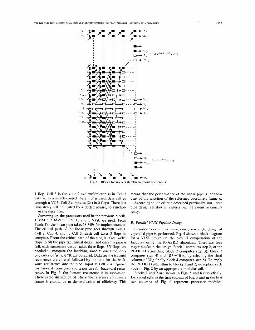
Fig. 4. Block diagram for VLSI on parallel computation of Jacobian

of two 3 X 1 vectors such as vector dot product and vector addition. We shall assume one scalar multiplication takes the same processing time as one scalar addition/subtraction in one floating-point operation (flop). Hence a vector dot product will take three flops, one multiplication and two additions. Table IV shows the number of MP's and flops for each of the MMP, MVP, VCP, and W A . We will use these MMP's, MVP's, VCP's, and WA's as building modular cells to complete our design of the Jacobian computation in a VLSI chip.

A . Linear VLSI Pipeline Design

Fig. 3 shows the data flow and systolic array implementation on the linear computation of the Jacobian using the generalized4 algorithm. In this linear pipeline design, five cells are needed. Cell 1 is a MMP. It computes (19) and (21) in 3 flops. Cell 2 is a MVP, which computes the second term of (20) and (22) in 3 flops. Cell 3 is a 2-to-1 multiplexer in which A, is a switch control. If A, =1, A is selected and k g , + l = 0. On the other hand, if A, = 0, B is selected; hence, the input data ( k R , and 2,) will be evaluated through a MVP. Cell 3 computes (23) in 2 flops. Cell 4 is a W A , which completes calculation of (20) and (22) in


k i i k+lR

Ltl i +.k L + I R

i+:

I I I I \

I I I I I I ; \ \ A-& LR, , ,

I I I I t) I I I I

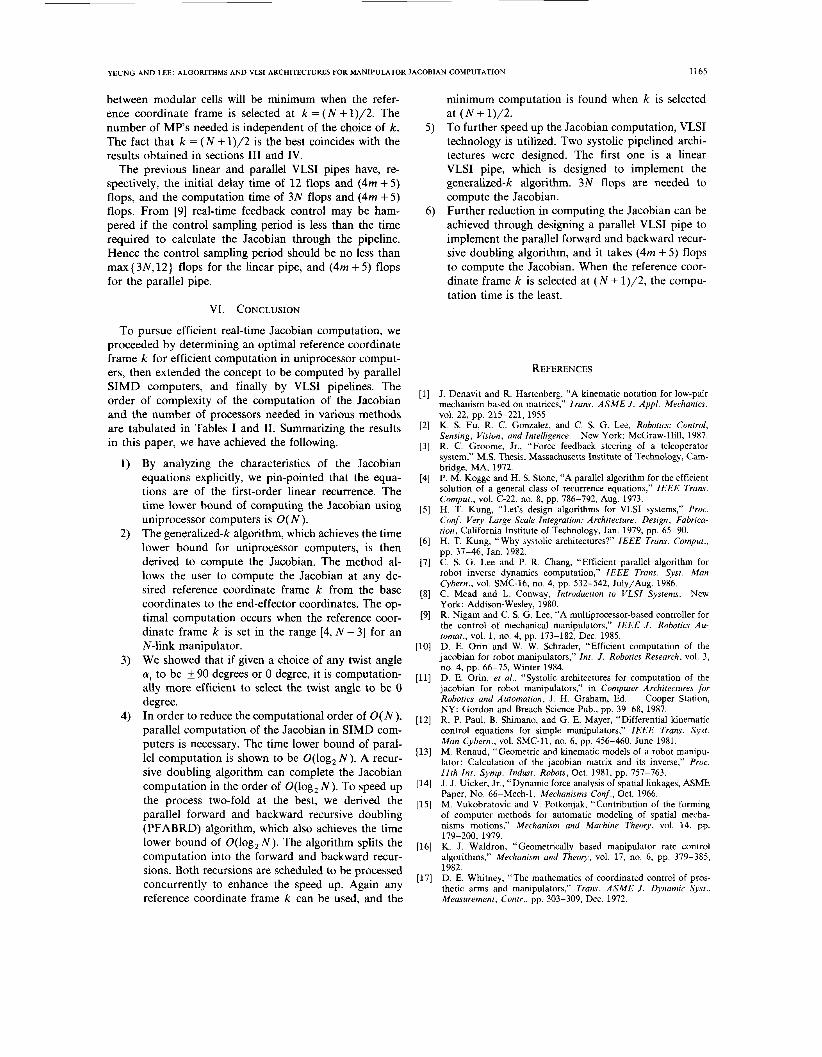
Fig. 5. Block 1 for any N with reference coordinate frame k

1 flop. Cell 5 is the same 2-to-1 multiplexer as in Cell 3 with A, as a switch control; here if B is used, data will go through a VCP. Cell 5 computes (24) in 2 flops. There is a time delay cell, indicated by a dotted square, to synchro- nize the data flow.

Summing up the processors used in the previous 5 cells, 1 MMP, 2 MVP’s, 1 VCP, and 1 W A are used. From Table IV, the linear pipe takes 18 MPs for implementation. The critical path of the linear pipe goes through Cell 1, Cell 2, Cell 4, and to Cell 5. Each cell takes 3 flops to compute. From the critical path of the pipe, it takes twelve flops to fill the pipe (i.e., initial delay), and once the pipe is full, each successive output takes three flops. 3N flops are needed to compute the Jacobian, since at one time, only one entry of kpl and k p , are obtained. Data for the forward recurrence are entered followed by the data for the backward recurrence into the pipe. Input at Cell 2 is negative for forward recurrence and is positive for backward recurrence. In Fig. 3, the forward recurrence is in succession. There is no distinction of where the reference coordinate frame k should be in the evaluation of efficiency. Ths

means that the performance of the linear pipe is independent of the selection of the reference coordinate frame k .

According to the criteria described previously, our linear pipe design satisfies all criteria but the extensive concurrency.

B. Parallel VLSI Pipeline Design

In order to exploit extensive concurrency, the design of a parallel pipe is performed. Fig. 4 shows a block diagram for a VLSI design on the parallel computation of the Jacobian using the PFABRD algorithm. There are four major blocks in the design. Block 1 computes step 2) of the PFABRD algorithm; block 2 computes step 3); block 3 computes step 4) and kPI* =kRIzo by selecting the third column of kRi; finally block 4 computes step 5). To apply the PFABRD algorithm to blocks 1 and 2, we replace each node in Fig. 2 by an appropriate modular cell.

Blocks 1 and 2 are shown in Figs. 5 and 6 respectively. Darkened cells in the first column of Fig. 5 and in the first two columns of Fig. 6 represent processor modules.


Fig. 6 . Block 2 for any N with reference coordinate frame k .

Columns thereafter represent operations at each successive time step, with darkened squares indicating numerical operations and open squares indicating null operations or pass of data. The arrows show how the data are being routed between processor modules. In block 1, each processor module is an MMP, and each time step takes 3 flops. There are ( N - 3) MMP's, and it takes m time steps or 3m flops to compute each new set of input data. In block 2, the darkened circles in column one are MVP's, and the darkened squares in column two are WA's. There are ( N - 2) MVP's and ( N - 3) WA's, and it takes ( m + 3) flops to compute.

Blocks 3 and 4 are shown in Figs. 7 and 8 respectively. Each square in these two figures represents a 2-to-1 multiplexer. A , is a switch control. When A; = 0, data at the top input will be used; when A, =1, data at the bottom input will be used. In block 3, when the top input is selected, the data will pass through an MVP, whereas in block 4, the data will pass through a VCP. In both cases, when the bottom input is selected, the output is the data at the input. Block 3 uses N MVPs and takes 3 flops to compute, whereas block 4 uses N VCP's and takes 2 flops to

r, "a;

Fig. 7. Block 3 for any N with reference coordinate frame k .

L. -

Fig. 8. Block 4 for any N with reference coordinate frame k .

compute. The total number of MP's needed to implement the parallel pipeline is (18N - 36).

From Fig. 4, the critical path of the parallel pipe starts from block 1 through block 2 to block 4. Hence the initial delay time of the parallel pipeline is (4m + 5) flops. Obvi- ously the initial delay time and the communication paths

YEUNG AND LEE: ALGORITHMS AND VLSI ARCHITECTURES FOR MANIPULATOR JACOBIAN COMPUTATION

~

1165

between modular cells will be minimum when the reference coordinate frame is selected at k = (N + 1)/2. The number of MP’s needed is independent of the choice of k . The fact that k = ( N + 1)/2 is the best coincides with the results obtained in sections I11 and IV.

The previous linear and parallel VLSI pipes have, respectively, the initial delay time of 12 flops and (4m + 5) flops, and the computation time of 3N flops and (4m + 5) flops. From [9] real-time feedback control may be ham- pered if the control sampling period is less than the time required to calculate the Jacobian through the pipeline. Hence the control sampling period should be no less than max {3N, 12) flops for the linear pipe, and (4m + 5) flops for the parallel pipe.

VI. CONCLUSION

To pursue efficient real-time Jacobian computation, we proceeded by determining an optimal reference coordinate frame k for efficient computation in uniprocessor computers, then extended the concept to be computed by parallel SIMD computers, and finally by VLSI pipelines. The order of complexity of the computation of the Jacobian and the number of processors needed in various methods are tabulated in Tables I and 11. Summarizing the results in this paper, we have achieved the following.

By analyzing the characteristics of the Jacobian equations explicitly, we pin-pointed that the equations are of the first-order linear recurrence. The time lower bound of computing the Jacobian using uniprocessor computers is O( N ) . The generalized-k algorithm, which achieves the time lower bound for uniprocessor computers, is then derived to compute the Jacobian. The method al- lows the user to compute the Jacobian at any desired reference coordinate frame k from the base coordinates to the end-effector coordinates. The optimal computation occurs when the reference coordinate frame k is set in the range [4, N - 31 for an N-link manipulator. We showed that if given a choice of any twist angle a, to be + 90 degrees or 0 degree, it is computationally more efficient to select the twist angle to be 0 degree. In order to reduce the computational order of O( N ) , parallel computation of the Jacobian in SIMD computers is necessary. The time lower bound of parallel computation is shown to be O(log,N). A recursive doubling algorithm can complete the Jacobian computation in the order of O(log, N ) . To speed up the process two-fold at the best, we derived the parallel forward and backward recursive doubling (PFABRD) algorithm, which also achieves the time lower bound of O(log, N ) . The algorithm splits the computation into the forward and backward recursions. Both recursions are scheduled to be processed concurrently to enhance the speed up. Again any reference coordinate frame k can be used, and the

minimum computation is found when k is selected at (N + 1)/2.

5 ) To further speed up the Jacobian computation, VLSI technology is utilized. Two systolic pipelined architectures were designed. The first one is a linear VLSI pipe, which is designed to implement the generalized-k algorithm. 3N flops are needed to compute the Jacobian. Further reduction in computing the Jacobian can be achieved through designing a parallel VLSI pipe to implement the parallel forward and backward recursive doubling algorithm, and it takes (4m + 5 ) flops to compute the Jacobian. When the reference coordinate frame k is selected at ( N + 1)/2, the computation time is the least.

6 )

REFERENCES

J. Denavit and R. Hartenberg, “A kinematic notation for low-pair mechanism based on matrices,’’ Trans. ASME J . Appl. Mechanics,

K. S. Fu, R. C. Gonzalez, and C. S . G. Lee, Robotics: Control, Sensing, Vision, and Intelligence. New York: McGraw-Hill, 1987. R. C. Groome, Jr., “Force feedback steering of a teleoperator system,” M.S. Thesis, Massachusetts Institute of Technology, Cam- bridge, MA, 1972. P. M. Kogge and H. S. Stone, “A parallel algorithm for the efficient solution of a general class of recurrence equations,” IEEE Trans. Comput., vol. C-22, no. 8, pp. 786-792, Aug. 1973. H. T. Kung, “Let’s design algorithms for VLSI systems,” Proc. Conf. Vety Large Scale Integration: Architecture, Design, Fahrica- tion, California Institute of Technology, Jan. 1979, pp. 65-90. H. T. Kung, “Why systolic architectures?” IEEE Trans. Comput., pp. 37-46, Jan. 1982. C. S. G. Lee and P. R. Chang, “Efficient parallel algorithm for robot inverse dynamics computation,” IEEE Trans. Syst. Man Cyhern., vol. SMC-16, no. 4, pp. 532-542, July/Aug. 1986. C. Mead and L. Conway, Introduction to VLSI Systems. New York: Addison-Wesley, 1980. R. Nigam and C. S. G. Lee, “A multiprocessor-based controller for the control of mechanical manipulators,” IEEE J . Robotics Au- tomat., vol. 1, no. 4, pp. 173-182, Dec. 1985. D. E. Orin and W. W. Schrader, “Efficient computation of the jacobian for robot manipulators,” Int. J . Robotics Research, vol. 3 , no. 4. pp. 66-75, Winter 1984. D. E. Orin, et al., “Systolic architectures for computation of the jacobian for robot manipulators,” in Computer Architectures for Robotics and Automation, J. H. Graham, Ed. Cooper Station, NY: Gordon and Breach Science Pub., pp. 39-68, 1987. R. P. Paul, B. Shimano, and G. E. Mayer, “Differential kinematic control equations for simple manipulators,” IEEE Tram. Syst. Man Cyhern., vol. SMC-11, no. 6, pp, 456-460, June 1981. M. Renaud, “Geometric and kinematic models of a robot manipulator: Calculation of the jacobian matrix and its inverse,” Proc. 11th Int. Symp. Indust. Robots, Oct. 1981, pp. 757-763. J. J. Uicker, Jr., “Dynamic force analysis of spatial linkages, ASME Paper, No. 66-Mech-1, Mechanisms Conf., Oct. 1966. M. Vukobratovic and V. Potkonjak, “Contribution of the forming of computer methods for automatic modeling of spatial mechanisms motions,” Mechanism and Machine Theoty, vol. 14, pp.

K. J. Waldron, “Geometrically based manipulator ratc control algorithms,” Mechanism and Theory, vol. 17, no. 6, pp. 379-385, 1982. D. E. Whitney, “The mathematics of coordinated control of pros- thetic arms and manipulators,” Trans. ASME J . Dynamic Syst., Measurement. Contr., pp. 303-309, Dec. 1972.

vol. 22, pp. 215-221, 1955.

179-200, 1979.


Tak Bun Yeung (M89) received the BSEE from the University of Texas, Austin in 1986, and the MSEE from Purdue University, West Lafayette, IN in 1987.

He was a Research Assistant in both of his undergraduate and graduate schools. His research interests include robotic control, parallel processing in computer architecture, and artifi- cial intelligence. He was with Seagate Technol- ogy Inc., Scotts Valley, CA in 1987-1989. He is now with LSI Logic Corp.

Mr. Yeung is a member of Tau Beta Pi, the National Society of Professional Engineers, and the Texas Society of Professional Engineers.

C. S. George Lee (S71-S78-M’78-SM’86) received the B.S. and M.S. degrees in electrical engineering from Washngton State University, Pull- man, WA in 1973 and 1974, respectively, and the Ph.D. degree from

Purdue University, West Lafayette, IN in 1978. In 1978-1985, he taught at Purdue University

and the University of Michigan. Since 1985, he has been with the School of Electrical Engineer- ing, Purdue University, where he is currently an Associate Professor. His current research interests include computational algorithms and architectures for robot control, intelligent multirobot assembly systems, and assembly planning.

Dr. Lee was an IEEE Computer Society Dis- tinguished Visitor in 1983-1986, and the Orga-

nizer and Chairman of the 1988 NATO Advanced Research Workshop on Sensor-Based Robots: Algorithms and Architectures. He is the Secre- tary of the IEEE Robotics and Automation Society, a technical editor of the IEEE Trunsactions on Robotics and Automation, a co-author of Robotics: Control, Sensing. Vision, and Intelligence (McGraw-Hill), and a co-editor of Tutorial on Robotics, (second ed), (IEEE Computer Society Press). He is a member of Sigma Xi and Tau Beta Pi.

Documents

Efficient parallel algorithms and VLSI architectures for manipulator Jacobian computation