Embed Size (px)
Citation preview
Rochester Institute of Technology Rochester Institute of Technology
RIT Scholar Works RIT Scholar Works
Theses
2006
Efficient job scheduling for a cellular manufacturing environment Efficient job scheduling for a cellular manufacturing environment
Joshua Dennie
Follow this and additional works at: https://scholarworks.rit.edu/theses
Recommended Citation Recommended Citation Dennie, Joshua, "Efficient job scheduling for a cellular manufacturing environment" (2006). Thesis. Rochester Institute of Technology. Accessed from
This Thesis is brought to you for free and open access by RIT Scholar Works. It has been accepted for inclusion in Theses by an authorized administrator of RIT Scholar Works. For more information, please contact [email protected].

Rochester Institute of Technology
EFFICIENT JOB SCHEDULING FOR A CELLULAR MANUFACTURING ENVIRONMENT
A Thesis
Submitted in partial fulfillment of the requirements for the degree of
Master of Science in Industrial Engineering
in the
Department of Industrial and Systems Engineering
Kate Gleason College of Engineering
by
Joshua S. Dennie
BS, Industrial Engineering
Rochester Institute of Technology, 2006

DEPARTMENT OF INDUSTRIAL AND SYSTEMS ENGINEERING
KATE GLEASON COLLEGE OF ENGINEERING
ROCHESTER INSTITUTE OF TECHNOLOGY
ROCHESTER, NY
CERTIFICATE OF APPROVAL
M.S. DEGREE THESIS
The M.S. Degree Thesis of Joshua S. Dennie
Has been examined and approved by the thesis committee
As satisfactory for the thesis requirement
For the Master of Science degree
Approved by:
Dr. Moises Sudit, Ph.D., Primary Advisor
Dr. Michael Kuhl, Ph.D., Advisor
ii
Abstract
An important aspect of any manufacturing environment is efficient job scheduling. With
an increase in manufacturing facilities focused on producing goods with a cellular manufacturing
approach, the need arises to schedule jobs optimally into cells at a specific time. A mathematical
model has been developed to represent a standard cellular manufacturing job scheduling problem.
The model incorporates important parameters of the jobs and the cells along with other system
constraints. With each job and each cell having its own distinguishing parameters, the task of
scheduling jobs via integer linear programming quickly becomes very difficult and time-
consuming. In fact, such a job scheduling problem is of the NP-Complete complexity class. In an
attempt to solve the problem within an acceptable amount of time, several heuristics have been
developed to be applied to the model and examined for problems of different sizes and difficulty
levels, culminating in an ultimate heuristic that can be applied to most size problems. The
ultimate heuristic uses a greedy multi-phase iterative process to first assign jobs to particular cells
and then to schedule the jobs within the assigned cells. The heuristic relaxes several variables and
constraints along the way, while taking into account the flexibility of the different jobs and the
current load of the different cells. Testing and analysis shows that when the heuristic is applied to
various size job scheduling problems, the solving time is significantly decreased, while still
resulting in a near optimal solution.
iii

TABLE OF CONTENTS
1 INTRODUCTION................................................................................................................. 1
1.1 PROBLEM STATEMENT ..................................................................................................... 1
1.2 LITERATURE REVIEW....................................................................................................... 9
2 FORMULATION................................................................................................................ 19
2.1 MATHEMATICAL MODEL ............................................................................................... 19
2.2 JOB SCHEDULING PROBLEM SIZES ................................................................................. 25
3 SOLUTION AND METHODOLOGY.............................................................................. 30
3.1 DEVELOPMENT AND EVOLUTION ................................................................................... 30
3.2 SMALL PROBLEMS ......................................................................................................... 31
3.3 MEDIUM PROBLEMS....................................................................................................... 33
3.4 LARGE PROBLEMS ......................................................................................................... 38
3.5 ULTIMATE HEURISTIC.................................................................................................... 43
4 RESULTS AND ANALYSIS ............................................................................................. 70
5 CONCLUSIONS AND FUTURE WORK........................................................................ 84
REFERENCES............................................................................................................................ 86
APPENDICES............................................................................................................................. 91
iv

1 Introduction
1.1 Problem Statement
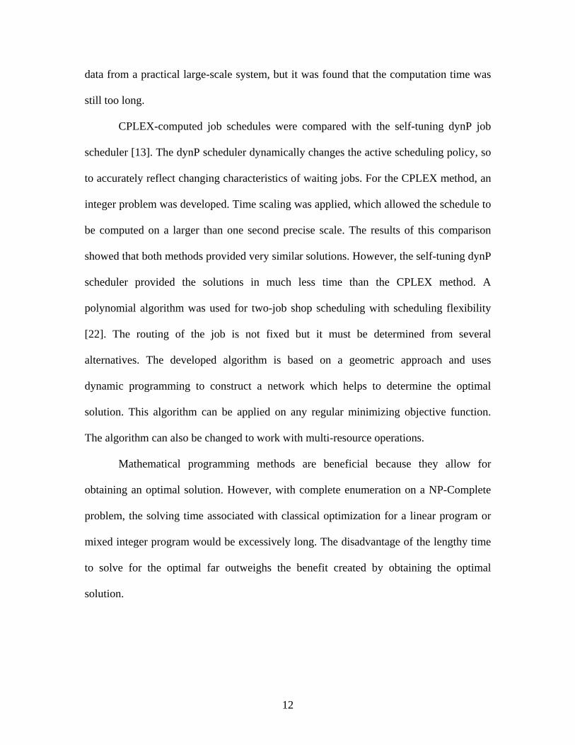
In today’s fast-paced and ever-changing society, significant value is placed on
efficiency, timing, and cost. Globalization is here to stay and will continue to impact the
way companies around the world conduct business. To remain competitive in comparison
to lower-cost manufacturers around the globe, more and more U.S. manufacturing
facilities are moving away from departmental manufacturing and turning towards cellular
manufacturing approaches, as shown in Figure 1.1, to improve efficiencies.
Generating
InspectionGrinding
Polishing
Ge
Gr Po
In Ge
In
Gr
In
Gr
Ge
Po
Po
Ge
Gr Po
In
Departmental Cellular
Figure 1.1: Shift from Departmental to Cellular Manufacturing
Within a departmental manufacturing environment, a job needs to travel through
several different work centers, each dedicated to completing a single step in the overall
process of manufacturing the job. This type of manufacturing setup lends itself to batch
and queue processing, resulting in jobs with excessive travel times and waiting times and
1
thus longer than necessary overall lead times. On the other hand, in a cellular
manufacturing environment, several work cells comprise the manufacturing space. Each
cell has the capability to complete each step in the process necessary to manufacture a
job. Once a job begins in a cell, each step in the overall process ensues until the job is
complete. This type of manufacturing setup promotes flow, resulting in minimal waiting
times and travel times, shorter lead times, and better customer responsiveness.
Optimax Systems, located in Ontario, NY, is an innovative manufacturer of
precision optics. They provide optical products, such as aspheres, cylinders, prisms,
spheres, and optical coatings. Optimax typically provides precision optics to customers
with a standard lead time between 6 weeks and 10 weeks. However, Optimax also offers
an expedited service that provides their customers optics in as little as one week at a
premium price. Two years ago, Optimax operated in a departmental manufacturing
environment. Each department specialized in one step of the process of making an optic.
For example, there was a grinding department that strictly focused on grinding the piece of
glass. After grinding, the piece would head to the polishing department to be polished.
This movement between the departments would continue until the optic completed each
assigned step in the designated process. This method of producing an optic was a huge
inefficiency. Each job would sit and wait on a shelf in a queue to be processed at each
department. Departments were not strategically located by distance, so when a job was
finished at one department, an employee had to walk the job to the next department and
set the job on the new department’s shelf. Furthermore, employees did not know which
job in the queue should be processed next. There was excessive and unnecessary work
accounted for in the process time, waiting time, and travel time. As the business continued
2
to grow, this type of manufacturing approach began to compromise Optimax’s key
strategies. It was necessary for Optimax to improve their approach to continue to be an
important player in the optics industry.
Recently, Optimax has undergone an enormous facelift. They have gone from
departmental, batch and queue processing to cellular, flow-focused manufacturing. Instead
of having several departments that only complete one step in the process, Optimax now
has several cells that complete all or most steps in the process. The next step in Optimax’s
transition is to optimize the scheduling of the jobs to the cells. Optimax has approximately
15 cells where jobs can be scheduled. Each cell has different parameters, including
employee skills, equipment cost, and capacity. Each job has different parameters, such as
potential profit, due date, specifications, and production requirements. Optimax is in need
of a job scheduling tool that allows for real-time scheduling, based on current jobs as well
as forecasted jobs. Furthermore, with frequent expedited orders, the job scheduler must be
able to dynamically handle the addition of these jobs in a short period of time where
capacity may be limited. The research performed in this thesis will aim to represent the
job scheduling problem that is currently faced by Optimax and many other companies that
operate in a cellular manufacturing environment. It will allow cellular manufacturers to
more optimally schedule jobs throughout their facility to keep up with their key strategies
and the ever-changing needs of their customers.
Most manufacturing facilities require some tool or technique to efficiently
schedule jobs through the facility, regardless of the manufacturing method. Inefficient
scheduling of jobs can compromise timeliness, quality, inventory, and most importantly
profits. A tool that schedules jobs in a cellular manufacturing environment would be
3

valuable to many facilities turning to this approach. The tool would allow manufacturers
to attempt to minimize cost. Potential byproducts of the tool would include the ability to
increase profits, while improving on-time delivery and customer responsiveness.
Additionally, the tool would provide additional forecasting capabilities. Manufacturers
could look ahead to see what type of cells have extra capacity or little capacity and quote
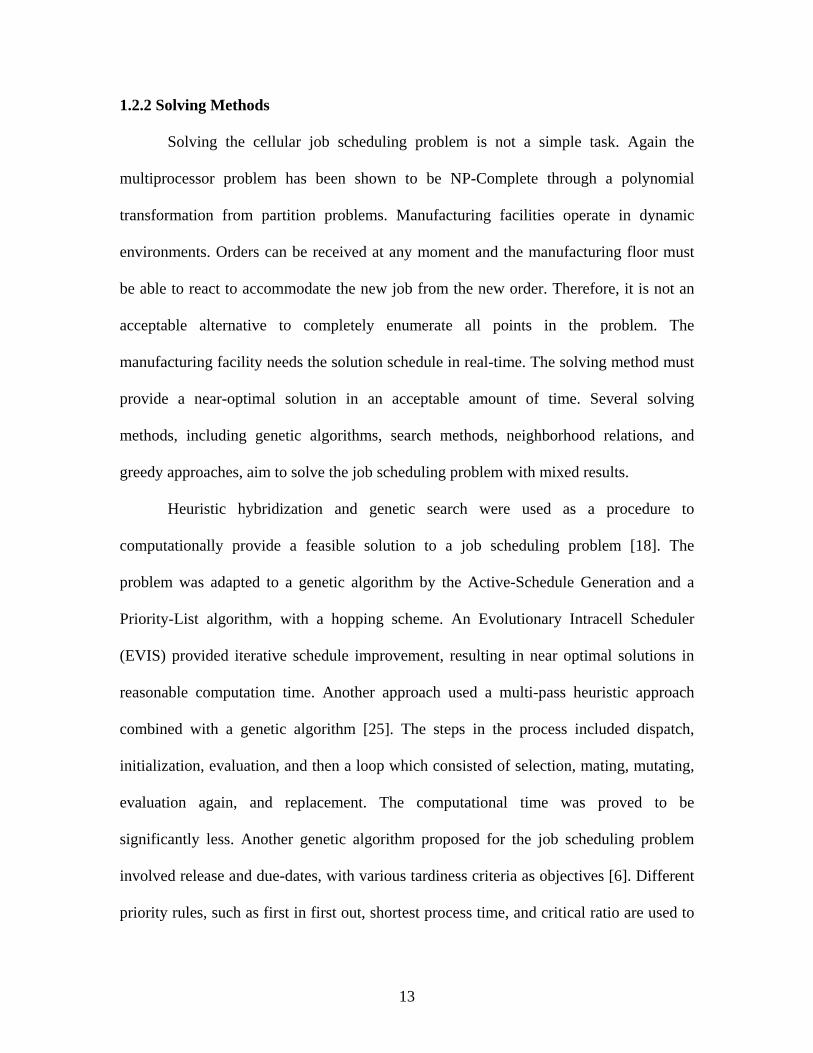
jobs accordingly, attempting to always keep a near full-capacity facility. Figure 1.2
displays the main concept of such a tool.
Figure 1.2: Job Scheduling Main Concept
There are several jobs, which are either in the work queue or forecasted to be
produced in the future. Each job has different properties or parameters as shown, which
may include completion time, early start date, due date, and production requirements.
Similarly, there are several different cells each with different properties, including
equipment, employee skills, feasibility, and cost. The goal of the job scheduler, through
PRODUCTION ORDERS Jobs in Jobs Queue Forecasted Cell 1
1 1Cell 2
2 2Job Scheduling
Algorithm
Cell p m n
Job Properties Cell Properties Completion Time • Equipment•
Employee Skills Early Start ••Due Date • Feasibility•Production Requirements Cost••
• Etc . • Etc.
4

the use of a job scheduler algorithm, is to optimally assign the jobs to the cells at a
specific time based upon an objective function that aims to maximize or minimize a
specific set of criteria.
Figure 1.3 is an example of a potential output that the job scheduler could
develop. Each job is assigned to a specific cell at a specific time. The duration of the job
is based upon the estimated completion time, as assigned by the process engineering
department or the manufacturing department. The chart shows the manufacturing facility
the blocks of time dedicated to producing jobs, as well as the blocks of time where there
is availability to potentially book an order for a job.
Time (days) t
0
Job #19Job #13
Job #7
Job #4
Job #15Job #8Job #10Job #5
Job #14Job #18 Job #12
Job #6Job #3
Job #17Job #16Job #9Job #11
Job #2
Job #1
1 2 3 4 5 6
Cell 1
Cell 2
Cell 3
Cell 4
Cell 5
Cell 6
Figure 1.3: Potential Job Scheduler Output
5

This output is not only helpful to the production control department, which may
schedule the jobs, but to the sales team as well. Since the job scheduler takes into account
forecasted jobs also, this type of output can also be used as a forecasting tool. When the
sales team is preparing a quote, they can look at the most up-to-date job schedule, to see
the plant capacity, and more specifically cell capacity, at any particular time. If the plant
or a specific cell has low availability at a particular time that a customer wants to place an
order, the sales team may choose to present a high quote to the customer. On the other
hand, if the plant or cell has high availability at a particular time, they may present a low
quote to ensure that they receive the job and keep the facility running at an acceptable
level. Therefore, if the facility receives an order during a low availability time period at a
higher price, the additional profit outweighs the extra cost, such as overtime, to complete
the job on time. Conversely, if the facility gains an order during a high availability time
period at a lower price, the sacrifice in profit is outweighed by keeping the workers busy
and not having to pay them without positive cash flow.
Providing such a schedule is not as simple as just placing jobs into cells at any
time. Several factors must be considered to ensure that all parameters of the problem are
met. For example, every job that needs to be scheduled has an associated due date driven
by the customer and agreed upon by the manufacturing company. Similarly, production
of a job may not be able to begin until a certain date, due to raw material or tooling
needs. Job to cell feasibility comes into play, as each cell may not have equal capabilities,
based on personnel and equipment, to produce a job. Therefore, each job will have a
corresponding list of potential feasible cells that the job can run in. The potential job
scheduler output also shows a few other important parameters of a cellular manufacturing
6

environment. Jobs are scheduled in only one cell, only one job is scheduled in a cell at
any particular time, and once a job is scheduled to begin it is produced without pre-
emption. All parameters of the different jobs and different cells, as well as the parameters
of cellular manufacturing can be described technically by a mathematical model, to be
displayed and discussed in more detail in Chapter 2. Through the use of integer linear
programming an optimal solution to a defined objective function can be achieved.
The mathematical representation of a cellular job scheduling problem is
intrinsically complex. To truly characterize the actual size of the job scheduling problem
faced by manufacturing facilities, such as Optimax, a representative number of jobs,
cells, and time periods are needed to provide a truly beneficial schedule. Several
parameters of the job and the cells must also be considered for added effectiveness.
Furthermore, due to the dynamic nature of manufacturing facilities, the scheduling
method must be a relatively quick process to be valuable. At every point that a new order
arrives, the job schedule must be rerun to accommodate the new job to supply the new
order. It is imperative that the job scheduling is as close to real-time scheduling as
possible. However, the size and complexity of the job scheduling problem significantly
impacts the time to solve for the optimal solution using integer linear programming via
the mathematical model. In fact, as David W. Sellers wrote in “A Survey of Approaches
to the Job Shop Scheduling Problem”, job scheduling problems are of the NP-Complete
complexity class [24]. It is practically impossible to investigate every potential feasible
solution, except in the easiest problem sets. More specifically, Garey and Johnson
showed that the multiprocessor scheduling problem is NP-Complete through a
polynomial transformation from partition problems [9]. The job scheduling problem to be
7
investigated in this thesis is a more specific case of the multiprocessor scheduling
problem in which the multiple cells represent multiple processors and tasks are
represented by jobs with their corresponding length (completion time) and deadline (due
date).
Therefore, the problem to be addressed in this thesis is realized. There is a need to
develop a job schedule for a cellular manufacturing facility. A mathematical model
allows for the cellular job scheduling problem to be represented, while integer linear
programming allows for the job schedule solution. However, the job schedule must be
realized in real-time due to the dynamic nature of manufacturing. Yet, due to the size and
complexity of the job scheduling problem as represented by the mathematical model, the
integer linear program cannot recognize even a feasible solution schedule, let alone an
optimal solution schedule, in a reasonable time frame to be of any value to the
manufacturing facility.
Since conventional optimization techniques cannot be used to solve the cellular
job scheduling problem faced by companies such as Optimax, it will be necessary to
develop alternative methods and apply them to the mathematical model to more
efficiently solve the scheduling problem to be of better use to the manufacturing facility.
The work in this thesis involves the creation of a mathematical model that represents a
cellular job scheduling problem and further work proves the complexity class of the
problem. The only way to guarantee an optimal solution is to completely enumerate all
points in the problem. Since this is not an acceptable alternative, due to time concerns,
the research in this thesis will investigate and examine heuristic methods that will create
more efficiency in the schedule solving process. The heuristic methods will aim to take
8

advantage of the structure of the problem detailed in Chapter 2 to allow for more
efficiency in the solving process. The heuristic methods will reduce the search space,
thereby attempting to reduce the overall solving time, while aiming to meet all of the
constraints of the problem. The attempted result is a near optimal solution schedule to a
NP-Complete job scheduling problem in a significantly decreased, acceptable amount of
computation time.
1.2 Literature Review
A tremendous amount of research and work has been done related to job
scheduling. A variety of heuristic procedures and classical optimization tools have been
used to solve several different job scheduling problems. In this literature review, several
methods of solving a wide range of difficult and complex job scheduling problems have
been investigated. The summary section will provide a brief explanation of the research
direction of this thesis.
1.2.1 Scheduling Methods
Much research has been done on job scheduling using decision rules. Research
was performed to determine optimal earliest time to start processing jobs [12]. Each job
must be processed on the same machine, with random time duration. Each job has its own
due date and a penalty for not meeting the due date, but also has an associated inventory
cost for being completed before the due date. Heuristics used in this problem focus on
decision-making regarding the random operations and cost parameters. The average
processing time combined with the central limit theorem is used to determine the
9
probability that a job will meet the due date. These probabilities and decision-making
rules can be used to determine the associated costs of completing the job early or late.
A team of researchers studied the development and implementation of a job
scheduler at a glass factory, where each job has a precedence constraint, an urgency
constraint, a due date, early date, and a late date [3]. Each job is made up of one or more
operations. An initial feasible solution is developed by quickly satisfying all precedence
and resource constraints, while intending to maximize machine utilization and minimize
work in process. After initialization, the jobs are assigned to machines by a priority
criterion and then an improving phase follows. Additional heuristics such as round robin,
parallel tasks, and work in next queue were investigated. A modified due date method
was decided upon which sufficiently satisfied due dates and work in progress.
Scheduling rules were developed for job shops that do not assume that the cost of
tardiness per unit is the same for each job and that the holding cost is not proportional to
the flowtime of the job [17]. A weighted slack rule was used that attempts to minimize
the maximum weighted tardiness and weighted variance of tardiness of jobs. A weighted
flow due date rule was also used, which attempts to yield the minimum values for the
maximum flow time and weighted variance of flow time of jobs. Another team
investigated the inapproximability of the no-wait job scheduling problem using the
makespan criterion [11]. In this type of environment there is no waiting allowed between
the executions of consecutive operations of the same job. Once a job is started, it must be
completed operation by operation, without pre-emption. It was found that the polynomial
time approximation scheme does not exist.
10

Decision rules are beneficial to job scheduling because they are relatively easy to
comprehend, fairly simple to relate to the problem, and normally improve solving time.
However, with problems of larger magnitude and complexity, the advantages of decision
rules tend to diminish. Decisions rules do not provide optimal solutions to problems, and
typically the more difficult the problems become, the further the decision rule solution is
from the optimal. Thus, developing a decision rule is not an ideal choice for a heuristic to
aid in solving the cellular job scheduling problem.
Mathematical programming is another scheduling method. Linear programming
and mixed integer programming are more specific methods that fall into this category.
Mathematical programming is advantageous because complete enumeration of the
problem can be achieved resulting in a true optimal solution. Researchers investigated
manufacturing systems where a high variety of products of different volumes must be
produced on a tight due date [15]. They used the feasibility function to schedule jobs in a
multi-machine random job shop. The objective is to balance the number of tardy and
early jobs, which will reduce the difference between the maximum and minimum lateness
of jobs. A simulation model with a multi-agent architecture was developed to allow for
comparison of a researched feasibility function method versus common scheduling rules.
The results show that the feasibility function is very beneficial for job scheduling.
An optimization-oriented method was used for simulation-based job scheduling,
which integrated capacity adjustment [4]. The goal of this method is to eliminate tardy
jobs within a manufacturing facility. The proposed method integrates parameter-space-
search-improvement into the scheduling procedure. To gain a near optimal solution, a
local search is completed to shorten the computation time. The method was tested using
11
data from a practical large-scale system, but it was found that the computation time was
still too long.
CPLEX-computed job schedules were compared with the self-tuning dynP job
scheduler [13]. The dynP scheduler dynamically changes the active scheduling policy, so
to accurately reflect changing characteristics of waiting jobs. For the CPLEX method, an
integer problem was developed. Time scaling was applied, which allowed the schedule to
be computed on a larger than one second precise scale. The results of this comparison
showed that both methods provided very similar solutions. However, the self-tuning dynP
scheduler provided the solutions in much less time than the CPLEX method. A
polynomial algorithm was used for two-job shop scheduling with scheduling flexibility
[22]. The routing of the job is not fixed but it must be determined from several
alternatives. The developed algorithm is based on a geometric approach and uses
dynamic programming to construct a network which helps to determine the optimal
solution. This algorithm can be applied on any regular minimizing objective function.
The algorithm can also be changed to work with multi-resource operations.
Mathematical programming methods are beneficial because they allow for
obtaining an optimal solution. However, with complete enumeration on a NP-Complete
problem, the solving time associated with classical optimization for a linear program or
mixed integer program would be excessively long. The disadvantage of the lengthy time
to solve for the optimal far outweighs the benefit created by obtaining the optimal
solution.
12
1.2.2 Solving Methods
Solving the cellular job scheduling problem is not a simple task. Again the
multiprocessor problem has been shown to be NP-Complete through a polynomial
transformation from partition problems. Manufacturing facilities operate in dynamic
environments. Orders can be received at any moment and the manufacturing floor must
be able to react to accommodate the new job from the new order. Therefore, it is not an
acceptable alternative to completely enumerate all points in the problem. The
manufacturing facility needs the solution schedule in real-time. The solving method must
provide a near-optimal solution in an acceptable amount of time. Several solving
methods, including genetic algorithms, search methods, neighborhood relations, and
greedy approaches, aim to solve the job scheduling problem with mixed results.
Heuristic hybridization and genetic search were used as a procedure to
computationally provide a feasible solution to a job scheduling problem [18]. The
problem was adapted to a genetic algorithm by the Active-Schedule Generation and a
Priority-List algorithm, with a hopping scheme. An Evolutionary Intracell Scheduler
(EVIS) provided iterative schedule improvement, resulting in near optimal solutions in
reasonable computation time. Another approach used a multi-pass heuristic approach
combined with a genetic algorithm [25]. The steps in the process included dispatch,
initialization, evaluation, and then a loop which consisted of selection, mating, mutating,
evaluation again, and replacement. The computational time was proved to be
significantly less. Another genetic algorithm proposed for the job scheduling problem
involved release and due-dates, with various tardiness criteria as objectives [6]. Different
priority rules, such as first in first out, shortest process time, and critical ratio are used to
13

improve the decision process. A permutation was developed which prioritizes any two
operations involved in the problem. They found that the capabilities of a genetic
algorithm decrease with an increasing problem size. With the help of a multi-stage
decomposition, the search space is reduced and the genetic algorithm works well.
Co-evolution and sub-evolution processes were introduced into a genetic
algorithm to tackle job scheduling [10]. Co-evolution was used to provide makespan and
idle time schedule criteria as the fitness functions of the operation-based genetic
algorithm. Subsequently, to provide high diversity for chromosome population, sub-
evolution was used so that the total job waiting time schedule constraint is the fitness
function for the genetic algorithm. With modifications to the standard deviation and
average of the computational results, this method shows robustness in solving the job
scheduling problem. Another genetic algorithm combined with a data mining based meta-
heuristic was proposed to solve the job scheduling problem [7]. This genetic algorithm
generates a learning population of feasible solutions, which are then mined by the mean
of classifier systems. The mining step produces decision rules that are transformed into a
meta-heuristic allowing for the efficient scheduling of operations to machines.
To build upon the efficiency of genetic algorithms, a team of researchers
proposed a hybrid heuristic genetic algorithm [8]. Scheduling rules, such as shortest
processing time and most work remaining were integrated into the genetic evolution
process. To improve the solution performance, the neighborhood search technique was
adopted as a supplementary procedure. The new hybrid genetic algorithm was proved to
be effective and efficient in comparison to other methods, including the neighborhood
search heuristic, simulated annealing, and traditional genetic algorithm. An immune
14

algorithm method was proposed that goes through a series of steps, including
initialization of antibodies, initialization of antigens, evaluation, generation, and
calculation [23]. The binary strings will gather to the point where the good value of the
fitness function is found. In comparison to genetic algorithms, the proposed immune
algorithms provide solutions in faster computation times.
A job scheduling method was investigated using group constraints, which means
that a job schedule for each line is decided upon and jobs dealing with the same process
must be grouped [14]. The research included a rapid generation of an initial feasible
solution by analyzing job flexibility according to an influential degree of a whole plan.
Improvement rules were used in combination with a tabu search, which resulted in
improvement of the total evaluation and confirmed effectiveness.
A stochastic strategy was developed for solving the job scheduling problem [16].
A tabu search was proposed and formalized to get a near optimal solution. The procedure
is based on an iterative “neighborhood search.” The tabu search keeps track of not only
short term information, but long term information as well. Two strategies, intensification
and diversification, are used to efficiently solve the problem in polynomial time. Another
search technique is based upon relaxing and then imposing the capacity constraints on a
few critical operations [24]. Subsequently, this technique is incorporated into a fast tabu
search algorithm. Results from this technique show that the approach is very effective, by
improving upon a range of test problems.
A heuristic was developed based on the tree search procedure for job scheduling
to minimize total weighted tardiness [5]. Each job has specific due dates and delay
penalties. A schedule is determined by minimizing the maximum tardiness subject to
15

fixed sub-schedules solved at each node of the search tree and the successor nodes are
generated, where the sub-schedules of the operations are fixed. Therefore, a schedule is
obtained at each node and the sub-optimum solution is determined among the obtained
schedules. Results show that the algorithm can find sub-optimum solutions with minimal
computation time.
An extension of the job scheduling problem was studied, where the job routings
are directed acyclic graphs that can model partial orders of operations and that contain
sets of alternative subgraphs consisting of several operations each [19]. A tabu search and
a genetic algorithm are used as heuristics, based upon two common subroutines. The first
inserts a set of operations into a partial schedule and the other improves a schedule with
fixed routing alternatives. The first subroutine relies on an efficient insertion technique,
while the second subroutine is a generalization of standard methods for job scheduling.
Results show that the methods proposed provide optimal solutions for three open
problems.
Methods were researched for manufacturing environments with random job
arrivals, non-deterministic processing times, and unpredictable events, such as machine
breakdowns. A complete multi-agent framework, including Lagrange multipliers, is used
to schedule jobs in this type of flexible workplace [1]. This approach combines real-time
decision making with predictive decision making, which can combat various different
scheduling problems. Another multi-agent scheduling method integrates earliness and
tardiness objectives for a flexible job shop, consistent with the just-in-time manufacturing
philosophy [27]. A job-routing and sequencing mechanism distinguishes jobs with one
16
operation left and jobs with multiple operations left. The results of the research show that
the proposed multi-agent scheduling method outperforms existing scheduling methods.
A job scheduling problem was researched, in which each job must process one
task on m machines [2]. The determination of the longest paths is the critical
computation. Heuristics are used by employing a neighborhood relation. To obtain a
neighbor, a single arc from a longest path is reversed and so these transition steps
guarantee a feasible schedule. Using logarithmic cooling schedules, the problem can be
solved within polynomial time.
A greedy heuristic was developed for the flexible job scheduling problem, which
is concerned with the assignment of operations to machines, as well as the sequence of
the operations [21]. The first job is fixed to start the polynomial algorithm. The next job,
with associated operations, is combined with the first job. The combinations are
organized in a Gantt chart according to the optimal schedule. The algorithm continues
until all jobs are formed into appropriate combinations, which gives the optimal job to
machine assignment.
A heuristic schedule was used based upon asymptotic optimality in probability for
open shops with job overlaps [20]. This approach focuses on scheduling applications
where parallel processing within a job is possible. The objective is to output an optimal
schedule while minimizing the summation of completion times of the jobs. The heuristic
orders the jobs by the average processing time of the operations of the job. A lower
bound on the optimal cost of each job is also introduced. The lower bound is used to
prove asymptotic optimality in probability of the heuristic when the processing times are
independently and identically distributed from any distribution with a finite variance.
17
Genetic algorithms, search methods, neighborhood relations, and greedy
approaches are all nice methods to solving the job scheduling problem. However, there is
no guarantee that any of these methods will achieve the goal of solving for a near-optimal
solution to a NP-Complete problem in an acceptable computation time to be of use to a
dynamic manufacturing environment. Therefore, this thesis will develop a heuristic that
can be applied to a mathematical model that represents a cellular job scheduling problem.
The heuristic will take advantage of the structure of the model to solve more efficiently,
while maintaining an acceptable level of optimality. The work will aim to leverage
several aspects of the mathematical model as well as specific characteristics of jobs and
cells contained in the scheduling problem to improve the efficiency of solving the cellular
job scheduling problem detailed in the mathematical model in Chapter 2.
18

2 Formulation
2.1 Mathematical Model
In this chapter, a developed mathematical model is presented to solve the job
scheduling problem that is representative of a cellular manufacturing environment. The
creation and design of the mathematical model is crucial to the types of heuristics that
can be applied to the problem. The research that is completed for the thesis will be based
upon this model. This mathematical model will schedule jobs in queue, as well as
forecasted jobs, to the best possible cell for production at the best possible time(s),
according to an objective function. It also describes important factors for jobs and cells,
using input parameters and constraints.
Notation
(1, 2,..., , 1, 2,..., )j job n n n n q= + + + (2.1)
• jobs in queue ( 1, 2,..., )n
• jobs forecasted ( 1, 2,..., )n n n q+ + +
(1, 2,..., )c cell p= (2.2)
(1,2,..., )t time r= (2.3)
Decision Variables
jcX = {1 if job j is assigned to cell c; 0 otherwise} (2.4)
jctY = {1 if job j is processed in cell c at time t; 0 otherwise} (2.5)
S j = time t that job j starts (2.6)
19

F j = time t that job j finishes (2.7)
Input Parameters
jd = time t that job j is due (2.8)
je = earliest time t to start job j (2.9)
ct j = length of time to complete job j (2.10)
jcf = job j to cell c feasibility (2.11)
• (1…feasible, 0…infeasible)
jcm = cost per unit time to produce job j in cell c (2.12)
Objective Function
( )* *jc jc jj c
Minimize Z X m ct=∑ ∑ (2.13)
Constraints
1jcc
X = ∀∑ j
c
(2.14)
,jc jcX f j≤ ∀ (2.15)
( )*jct jct
Y TIME X j≤∑ ,c∀
,c t
(2.16)
1jctj
Y ≤ ∀∑ (2.17)
( )* * 1jct jct jt Y TIME Y S j c t+ − ≥ ∀ , , (2.18)
20

*j jct , ,F t Y j c t≥ ∀ (2.19)
jct jcc t
Y ct= ∀∑∑ j (2.20)
jSe jj ∀≤ (2.21)
jdF jj ∀≤ (2.22)
jctSF jjj ∀−=− 1 (2.23)
The mathematical model is clearly represented by three indicies; job, cell, and
time. The job notation, in 2.1, describes the list of jobs to be scheduled, with
accompanying actual job numbers. The cell notation, in 2.2, describes the list of cells that
jobs can be scheduled in, with accompanying cell names. The time notation, in 2.3,
describes the length of the discetized time periods, with accompanying time units. The
three indicies will be used to schedule a job to a specific cell over specific time periods.
The mathematical model involves four decision variables. The assignment
variable, shown in 2.4, is a two-dimensional (job, cell) binary variable that is equal to 1 if
a job is assigned to a specific cell or 0 otherwise. Similarly, the schedule variable, shown
in 2.5, is a three-dimensional (job, cell, time) binary variable that is equal to 1 if a job is
assigned to a specific cell during a particular time. Otherwise the value of the variable is
equal to 0. The start time variable, shown in 2.6, gives the time period that a job is
scheduled to begin production, while the finish time variable, shown in 2.7, gives the
time period that a job is scheduled to complete production.
The first job parameter that will be included in the mathematical model is due date,
shown in 2.8. Due date is one of the main driving forces behind the scheduling of jobs.
21

Simply put, it provides a worst-case date for when the job must be completed that aligns
with the needs of the customer. The customer expects the job to be delivered in
accordance with the due date. If the job is not delivered on time it is likely that the
company’s reputation can be damaged or profits can be sacrificed. Therefore, due dates
supply a simple to understand baseline date that is to be met for each job.
Early start date, shown in 2.9, is another job parameter that will be included in the
mathematical model. Early start date operates in a similar manner to due date. It provides
a best-case date for when a job can actually begin manufacturing. Early start date is a
critical job parameter mainly for a few reasons. First, it comes into play with forecasted
jobs that have yet to be confirmed for production. Manufacturing facilities do not want to
begin production of a forecasted job, until there is a better understanding of whether the
job will truly come to fruition. Secondly, inventory concerns come into play. It costs time
and money to store products in inventory on both the producer and customer sides. The
producer doesn’t want the job to be completed too early, resulting in a significant finished
goods inventory cost. Similarly, the customer doesn’t want the product too soon before it
is needed, resulting in additional storage costs. Finally, the early start date is put in place
due to the availability of specialized tools and materials. Typically, there is some sort of
lead time associated with the delivery of raw materials or tools needed for the production
of a job. Obviously, the job cannot begin until the necessary materials and tools are
available to the cell.
The final job-specific parameter to be included in the mathematical model is
completion time, shown in 2.10. The completion time is defined as the number of time
periods that a job will take for full production. For the purposes of this research,
22

completion time will be of a deterministic nature. Typically, the completion time of a
particular job would be determined by historical manufacturing data and information
associated with similar past jobs. The completion time is important because is provides the
block of time that a job must be scheduled for within a cell.
One cell input parameter that will be included in the mathematical model is known
as feasibility, shown in 2.11. Each job is either feasible or infeasible with each of the
different cells. This method provides a simple, straight forward approach to assigning
feasibility of a job to a cell. Additionally, this method allows for compiling several
different parameters into one parameter. The feasibility looks at many job parameters and
cell parameters to determine the feasibility relationship between each job and each cell. At
a minimum, the feasibility parameter takes into account specifications and production
requirements of a job and the equipment and employee skills of a cell. If the necessary
specifications and production requirements of a job match the equipment and employee
skills that are located in a cell, the job is feasible for production in that particular cell. On
the other hand, if the specifications and production requirements of a job don’t align with
the equipment and employee skills of a cell, that relationship is infeasible.
The final parameter, cost, shown in 2.12, provides a cost per time unit of
manufacturing a particular job in a specific cell. Cost incorporates several different
smaller costs associated with the manufacturing of a job in a cell. For example, each cell
has an employee wage cost associated with it. Some cells have multiple employees and/or
high-skilled employees that increase the wage cost. In addition, there is a burden cost
associated with each cell that may incorporate equipment cost and square footage cost.
The cost parameter also serves as an extension of the feasibility parameter. Although the
23
feasibility parameter is binary, job to cell feasibility is actually not so cut and dry. For a
particular job, there are some cells that are very good matches for production, there are
some cells that are impossible for production, and there are some cells in between that
could produce the job if necessary. Thus, the cost parameter comes into play with the cells
in between to allow for some continuity within feasibility. For instance, Job A matches the
parameters of Cell X very well. More often than not, Job A should be scheduled for
production in Cell X. However, Job A could be scheduled to Cell Y, if Cell X is full and
production is absolutely necessary by a certain date. The cost parameter associated with
the Job A to Cell Y relationship can be inflated to an appropriate level to allow Job A to
be scheduled to Cell Y, but simultaneously ensures that it happens only if absolutely
necessary.
The goal of any firm or company should be to maximize profit. However since
profit is difficult to represent from a scheduling perspective, the objective, shown in 2.13,
in this model is to schedule the jobs accordingly to minimize the overall cost associated
with producing the set of jobs in their assigned cells.
There are several conditions or constraints that must be met while scheduling the
jobs, in accordance with cellular manufacturing principles. First each job must be
produced entirely within only one cell, as represented in 2.14 and known as the “one cell
only” constraint. The assigned cell for a particular job must be a feasible cell, as
represented in 2.15 and known as the “cell feasibility” constraint. If a job is not assigned
to a particular cell, it can’t be scheduled in that cell, as represented in 2.16 and known as
the “schedule only if assigned” constraint. TIME is defined as the value of the latest time
in the set of time periods. Furthermore, within one cell, only one job can be worked on at
24

any particular time, as represented in 2.17 and known as the “one job at a time”
constraint. The starting time of a job is determined using the “starting time” constraint,
shown in 2.18, while the finishing time of a job is determined using the “finishing time”
constraint, shown in 2.19. A job must be scheduled for the entirety of the designated
completion time, as represented in 2.20 and known as the “scheduled time equals
completion time” constraint, while not being scheduled before its early start date, as
represented by 2.21 and known as the “early start date” constraint, or after its due date, as
represented by 2.22 and known as the “due date” constraint. Once a job is scheduled for a
particular time, it must remain in the cell until completion, in a sequential manner, as
represented in 2.23 and known as the “sequential time” constraint.
For the purpose of this thesis, the mathematical model has been formulated using
a software program known as Optimization Programming Language (OPL), version 3.7,
from a company called ILOG. The problem will then be solved using OPL and a solution
tool known as CPLEX. The baseline OPL model along with a glossary of terms to allow
for easy translation can be found in Appendix A.
2.2 Job Scheduling Problem Sizes
There are an endless number of job scheduling problems that arise from the
numerous combinations of input parameters, as well as the quantity of jobs, cells, and
time periods. To address this concern, for the purpose of this work, the job scheduling
problems will reflect the general state of job scheduling problems at facilities that operate
in a cellular manufacturing environment, such as Optimax Systems, Inc., described in
Chapter 1.
25

Typically, at any given time, the manufacturing facility is approximately
operating at 85% capacity. This means that the jobs currently planned to be produced
occupy 85% of the facility’s physical work time to complete the jobs. Of course, this
number is not constant and can fluctuate higher and lower depending on the market
demand for goods.
A 10-week or 2.5-month time frame looking forward portrays the window of time
that most facilities are concerned with to be scheduled. This allows for scheduling of jobs
with a 6-10 week lead time. It also allows for scheduling of expedited jobs that must be
scheduled with shorter lead times, potentially delaying other jobs.
The completion time of jobs is dependent on the quantity of parts in the job and
the difficulty of the job. Simple jobs may take as little as one day to complete, while
more difficult jobs can take upwards of 5 days or a full work week for completion. Some
jobs can begin to be produced as soon as the order is confirmed. However, some jobs
must be delayed due to material, tool, inventory, or forecasting reasons. The early start
date takes these concerns into account, while adjusting the due date to provide a
reasonable window of time for completion for any particular job.
Cell break points of 5 cells, 10 cells, and 15 cells will be used for
experimentation. Obviously, jobs are not feasible to all cells, and a job may be a better fit
for a certain cell than another cell. On average, jobs are allocated as feasible to 40% of
the cells. This does not mean that each job is feasible to 40% of the cells, but overall 40%
of the cells are feasible for all the jobs. For example, in the case of a 5-cell problem, Job
1 is feasible to only one cell, but Job 2 is feasible to three cells. For Job 2, each of the
three feasible cells may not be equally feasible. This is where cost comes into play. The
26
most difficult feasible cell will be allocated a higher cost in comparison to the easier
feasible cells.
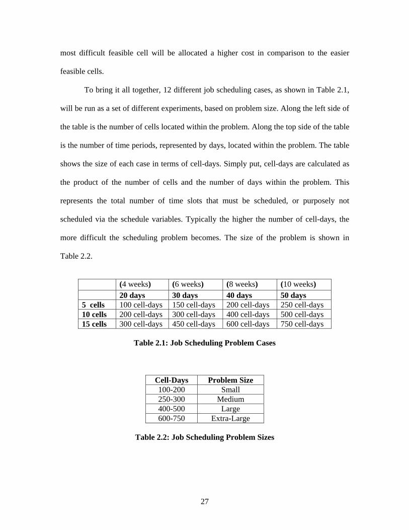
To bring it all together, 12 different job scheduling cases, as shown in Table 2.1,
will be run as a set of different experiments, based on problem size. Along the left side of
the table is the number of cells located within the problem. Along the top side of the table
is the number of time periods, represented by days, located within the problem. The table
shows the size of each case in terms of cell-days. Simply put, cell-days are calculated as
the product of the number of cells and the number of days within the problem. This
represents the total number of time slots that must be scheduled, or purposely not
scheduled via the schedule variables. Typically the higher the number of cell-days, the
more difficult the scheduling problem becomes. The size of the problem is shown in
Table 2.2.
(4 weeks) (6 weeks) (8 weeks) (10 weeks) 20 days 30 days 40 days 50 days 5 cells 100 cell-days 150 cell-days 200 cell-days 250 cell-days 10 cells 200 cell-days 300 cell-days 400 cell-days 500 cell-days 15 cells 300 cell-days 450 cell-days 600 cell-days 750 cell-days
Table 2.1: Job Scheduling Problem Cases
Cell-Days Problem Size 100-200 Small 250-300 Medium 400-500 Large 600-750 Extra-Large
Table 2.2: Job Scheduling Problem Sizes
27
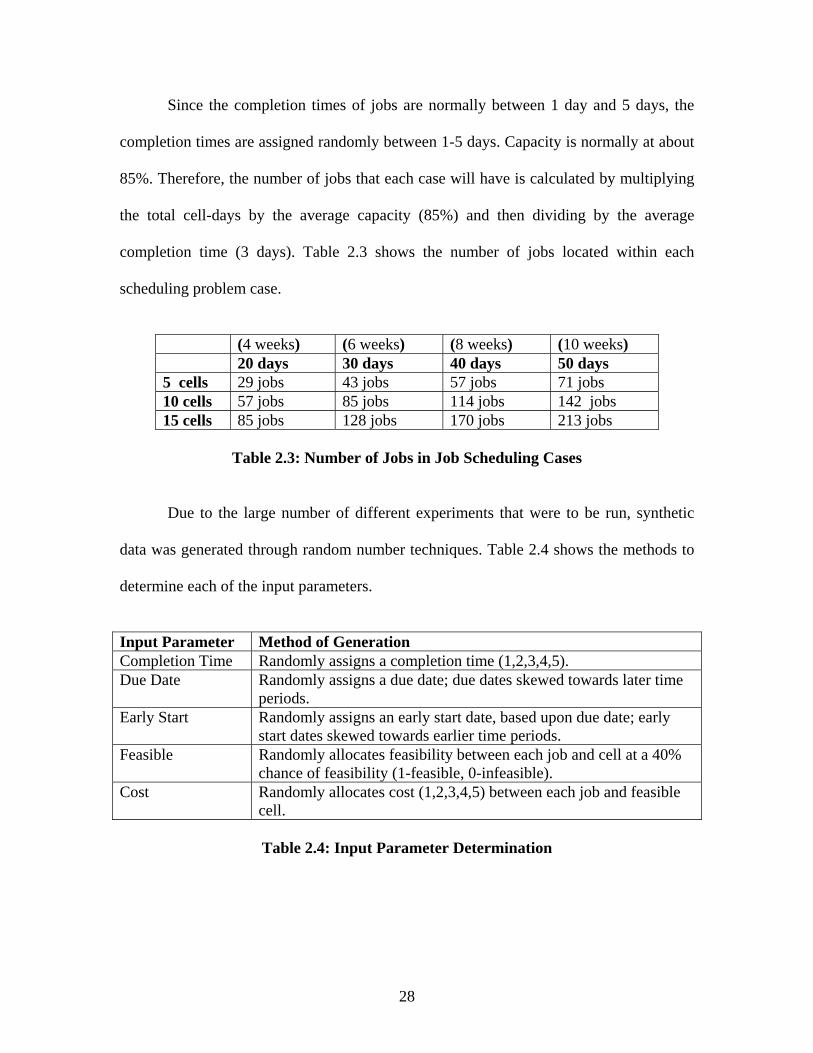
Since the completion times of jobs are normally between 1 day and 5 days, the
completion times are assigned randomly between 1-5 days. Capacity is normally at about
85%. Therefore, the number of jobs that each case will have is calculated by multiplying
the total cell-days by the average capacity (85%) and then dividing by the average
completion time (3 days). Table 2.3 shows the number of jobs located within each
scheduling problem case.
(4 weeks) (6 weeks) (8 weeks) (10 weeks) 20 days 30 days 40 days 50 days 5 cells 29 jobs 43 jobs 57 jobs 71 jobs 10 cells 57 jobs 85 jobs 114 jobs 142 jobs 15 cells 85 jobs 128 jobs 170 jobs 213 jobs
Table 2.3: Number of Jobs in Job Scheduling Cases
Due to the large number of different experiments that were to be run, synthetic
data was generated through random number techniques. Table 2.4 shows the methods to
determine each of the input parameters.
Input Parameter Method of Generation Completion Time Randomly assigns a completion time (1,2,3,4,5). Due Date Randomly assigns a due date; due dates skewed towards later time
periods. Early Start Randomly assigns an early start date, based upon due date; early
start dates skewed towards earlier time periods. Feasible Randomly allocates feasibility between each job and cell at a 40%
chance of feasibility (1-feasible, 0-infeasible). Cost Randomly allocates cost (1,2,3,4,5) between each job and feasible
cell.
Table 2.4: Input Parameter Determination
28
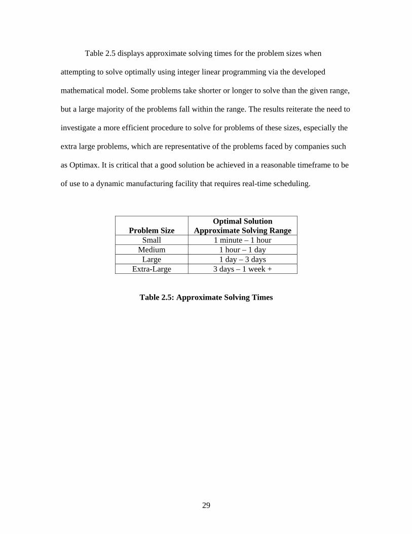
Table 2.5 displays approximate solving times for the problem sizes when
attempting to solve optimally using integer linear programming via the developed
mathematical model. Some problems take shorter or longer to solve than the given range,
but a large majority of the problems fall within the range. The results reiterate the need to
investigate a more efficient procedure to solve for problems of these sizes, especially the
extra large problems, which are representative of the problems faced by companies such
as Optimax. It is critical that a good solution be achieved in a reasonable timeframe to be
of use to a dynamic manufacturing facility that requires real-time scheduling.
Problem Size
Optimal Solution Approximate Solving Range
Small 1 minute – 1 hour Medium 1 hour – 1 day
Large 1 day – 3 days Extra-Large 3 days – 1 week +
Table 2.5: Approximate Solving Times
29

3 Solution Methodology
3.1 Development and Evolution
The formulation of the mathematical model significantly impacts the types of
heuristics that can be applied to more efficiently solve the problem. The goal of the
mathematical model was not only to represent the job scheduling problem of a cellular
manufacturing facility, but to also allow the acceptance of different potential heuristic
procedures. Once again, the objective of this job scheduling problem is to schedule all the
jobs to a specific cell over a designated amount of time, while minimizing overall cost. In
simplest form, only the schedule variable, Yjct, is necessary to deliver all the information
to the manufacturing facility. The schedule variable shows exactly what job is assigned to
what cell and at what time(s), through a binary notation. However, with the addition of
the assignment variable, Xjc, the problem can easily be broken down into two separate
phases, assigning (jobs to cells) and scheduling (jobs to times within assigned cells). The
ability to split the problem into separate phases, assigning and scheduling, enables the
problem to be simplified through heuristic techniques. The heuristic will take advantage
of the structure of the model to solve more efficiently, while maintaining an acceptable
level of optimality. The developed heuristic will work to leverage the structure of the
mathematical model of jobs and cells contained in the scheduling problem to improve the
efficiency of solving the cellular job scheduling problem detailed in the mathematical
model in Chapter 2.
A heuristic method does not just suddenly develop out of nowhere on its own.
Instead the heuristic evolves from several different ideas through a process of repetitive
trial and error, as well as significant experimentation. There are numerous ways to go
30
about creating a heuristic, including relaxing constraints and relaxing integer variables.
The size and difficulty of a job scheduling problem greatly impacts the capability of a
heuristic when applied to the problem. The evolution of the heuristic to be detailed in this
thesis started with attempts to solve small-sized problems and slowly progressed to
solving larger-sized problems. The techniques developed in the smaller problems are
adjusted and expanded upon so that they can be applied to the larger problems.
3.2 Small Problems
With 200 cell-days or less, small problems are the simplest class to be examined
within this research. Small problems are likely the type of problem that a department area
or small company, with smaller lead times, would face on a consistent basis. More often
than not, small problems can be solved optimally through use of the baseline
mathematical model, without the use of any heuristic procedures. Nevertheless, the
computation time for solving optimally can range anywhere from a couple seconds to a
couple minutes to a couple hours. By using just a few simple procedures, the problem-
solving can be quickened and a feasible (potentially optimal) solution can be found in a
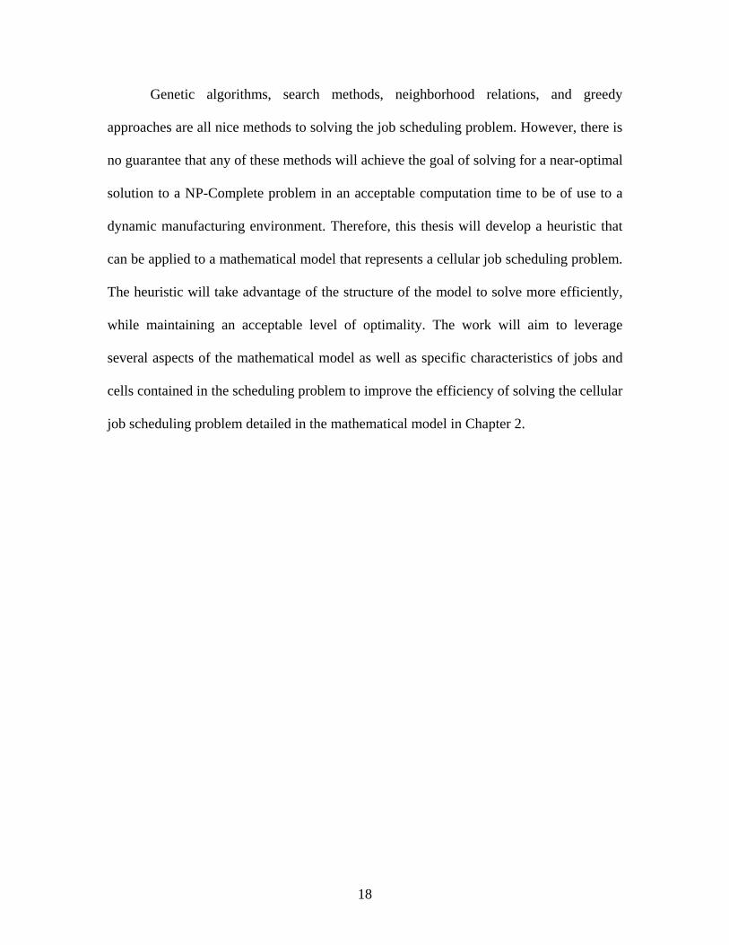
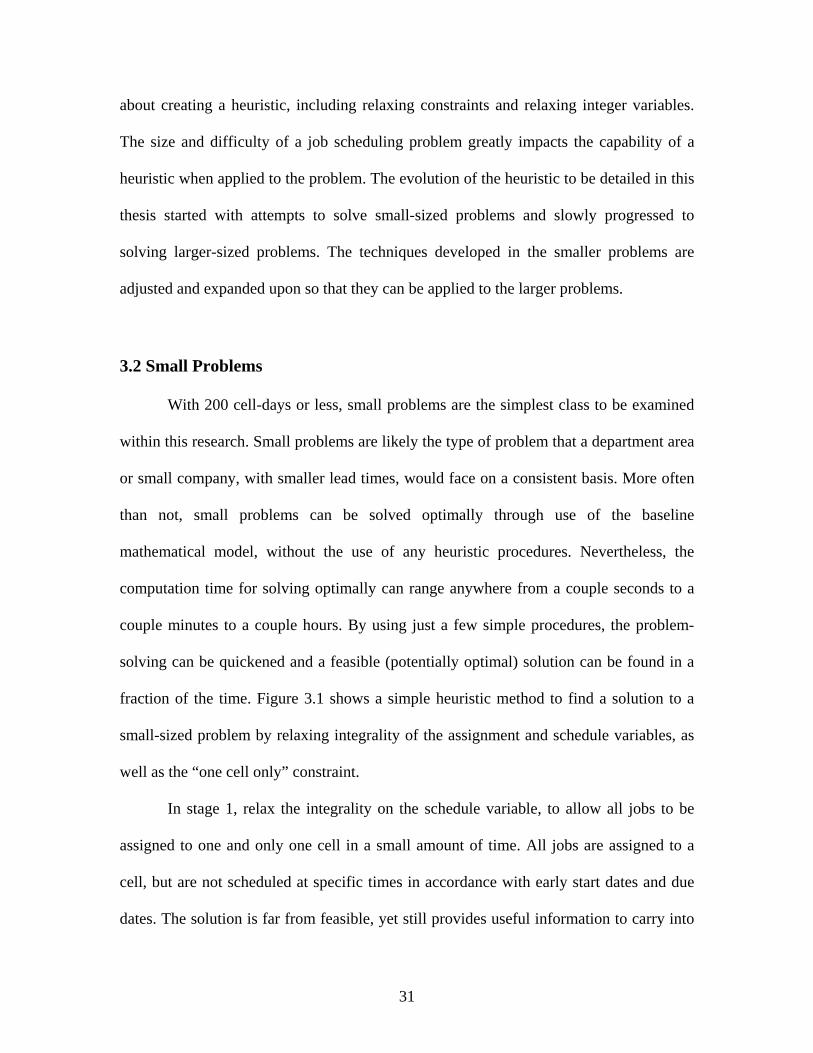
fraction of the time. Figure 3.1 shows a simple heuristic method to find a solution to a
small-sized problem by relaxing integrality of the assignment and schedule variables, as
well as the “one cell only” constraint.
In stage 1, relax the integrality on the schedule variable, to allow all jobs to be
assigned to one and only one cell in a small amount of time. All jobs are assigned to a
cell, but are not scheduled at specific times in accordance with early start dates and due
dates. The solution is far from feasible, yet still provides useful information to carry into
31
the next stage. Transform each job-to-cell assignment variable into a constraint and add
them to the mathematical model to be used in stage 2.
Run Model
Stage 1:Assign all jobs to only one cell
1. Relax integrality on schedule variable
Stage 2:Schedule jobs within assigned cells
1. Transform job-to-cell assignment variable into constraints2. Relax integrality on assignment variable3. Change schedule variable back to integer form4. Allow multiple cell assignments via constraint
Are all jobs still assigned to only
one cell?
Run Model
Optimal Solution
YES
NO
Stage 3...n:Reschedule infeasible jobs
1. Eliminate job-to-cell assignment constraint for job(s) that were assigned to multiple cells
Run Model
Are all jobs assigned to only
one cell?
Heuristic Feasible Solution
YES
NO
Figure 3.1: Heuristic Strategy #1 – Small Problem
For stage 2, change the schedule variable back to its original integer form. Instead
relax the integrality on the assignment variable. In addition, relax the “one cell only”
constraint, to now allow for multiple cell assignments per job. Since in stage 1, early start
dates and due dates were not met, it is possible that all jobs assigned to a cell cannot be
appropriately scheduled in that particular cell. Therefore, by relaxing the “one cell only”
constraint, a job can be assigned and scheduled over two cells, if necessary.
After running the model again, if a solution is found where all jobs are assigned to
only one cell, the solution is optimal. If one or more jobs are assigned to multiple cells,
32

the solution is infeasible. Eliminate the job-to-cell assignment constraint added in stage 2
for the job(s) that are assigned to multiple cells and run the model again. Continue this
process until all jobs are assigned to one and only one cell. At this point, a feasible
solution is found, with the possibility that the solution is still optimal. Normally, this
entire heuristic process takes no more than a few seconds depending on the magnitude of
the problem.
Beneficially, this heuristic procedure provides an optimal or feasible solution in a
short amount of computation time on a very consistent basis with problems of small
magnitude. On the other hand, the heuristic can get caught in a large loop at stage 3, if
jobs continue to get assigned to multiple cells. This leads to a longer computation time
and backtracks to a more difficult problem. Furthermore, as the size of the problem at
hand increases, the ability of this heuristic to provide a solution quickly diminishes. A
more difficult problem spells more cells, more time, and more jobs. With an increase in
the number of jobs, this heuristic has difficulty assigning all the jobs to one cell in stage
1. Additionally, as the number of cell-days increases, it is more difficult to schedule the
jobs even if they can be assigned to distinct cells.
3.3 Medium Problems
In one way or another, medium problems experience a slight increase in the
number of jobs, number of cells, or the number of time periods. Due to the increase of the
dimensions of the problem, the strategy to acquire a solution must be adapted in relation
to smaller problems. Medium problems still have a slim chance to be solved optimally,
without any modifications to the baseline mathematical model. Nonetheless, the solving
33

process could take several minutes or even several hours. By applying a three-stage
heuristic procedure to this size problem, the solving time can be significantly decreased,
while not sacrificing considerable optimality to the objective. The crucial part of this
heuristic is obtaining an initial feasible solution to the adjusted problem at hand as soon
as possible. After an initial feasible solution is found, useful bits of information from the
adjusted feasible solution can be adapted to the next stage to speed along the overall
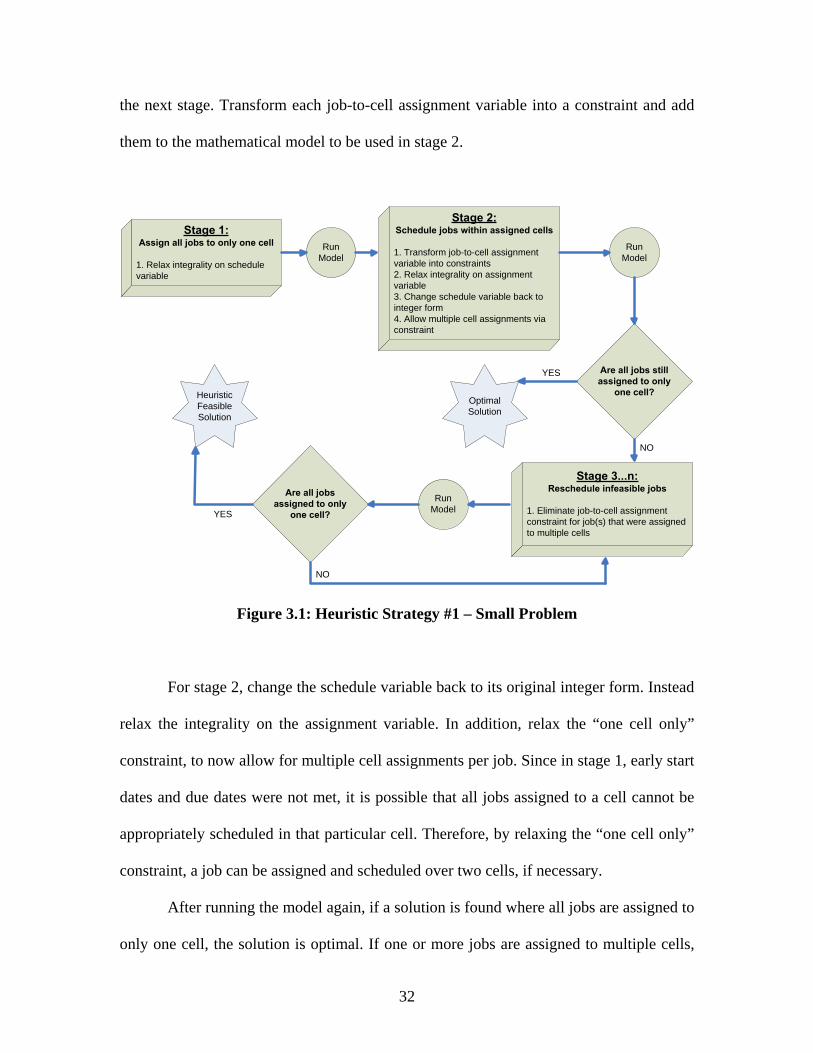
solution process. Figure 3.2 shows the basic concept of the heuristic procedure.
Figure 3.2: Heuristic Strategy #2 – Medium Problem
34

Stage 1 involves changing the assignment variable and the schedule variable from
the integer form to the continuous form. Since this is no longer an integer program
whatsoever, an optimal solution is quickly obtained in just a few seconds. Although this
solution is far from a good solution for the true problem, it provides useful information to
carry on to the next stage.
In stage 2, the assignment variables from the stage 1 solution are analyzed. If a
job-to-cell assignment variable is equal to 1, it represents a high importance, relative to
the objective function, to schedule that job within that cell. Thus the job-to-cell
assignment actually becomes a constraint and is added within the model. This occurs for
all job-to-cell assignment variables that are equal to 1. Usually between 60%-70% of jobs
are assigned solely to one cell after stage 1.
Before the model is run again, the schedule variable is changed back to a binary
integer variable. This is a step in the right direction towards the true mathematical model,
as jobs now must be scheduled for an entire time period, instead of portions of a time
period. Additionally, the “one cell only” constraint is modified to allow for multiple cell
assignments. Therefore, jobs can be assigned to more than just one cell. By changing this
constraint, a feasible solution is found significantly faster than by forcing all of the jobs
to be scheduled to only one cell. Now the model can be run once again.
The model has now been turned into a partial integer program. Understandably,
the solving process is more time-consuming. Nevertheless, since many of the jobs have
already been assigned to a distinct cell, a feasible solution is obtained to the problem at
hand, typically within about a minute. Next, a balancing act must occur as the longer
program runs, the better the solution becomes, resulting in better information to carry into
35
the next stage. After approximately 2 minutes, if the solution is not yet optimal, but is
feasible, the model can be stopped and the procedure can continue with the best feasible
solution. Two minutes was chosen for several reasons. First, time is not compromised
significantly as two minutes is a very short amount of time for such a problem of this
magnitude. Secondly, a feasible solution can typically be found within two minutes for
this set of problems. Finally, after two minutes, the solution doesn’t have much more
room for improvement, but the time to achieve the improvement is significant. In the
unlikely case that a feasible solution is not found within 2 minutes, allow the model to
continue to run until a feasible solution is found.
In stage 3, the schedule variables from the stage 2 solution are analyzed. If a job is
scheduled in only cell, the schedule variables for that job are transferred into the
mathematical model in the form of constraints. After stage 2, about 75% of the jobs will
be scheduled appropriately in one cell. This represents the eventual schedule for these
jobs. However, before it can become the actual schedule, the remaining jobs must be
scheduled. Since the schedule variables have been added to the mathematical model, all
assignment variable constraints that were added in stage 2 can be removed. The
remaining jobs are able to be scheduled to any feasible cell.
Before the model is run again, the mathematical model is changed back to its
original form. The assignment variable is changed back to integer form. In addition, the
“one cell only” constraint is changed back to allow for only one cell assignments. Now,
the model can be run again in an attempt to find a good feasible solution to the true job
scheduling problem. Typically, an optimal solution is found within one minute. The
36
model can be stopped after two minutes with a feasible solution, in the unlikely case that
the model hasn’t yet found an optimal solution. The best feasible solution is used.
Due to the fact that several jobs have already been locked into place after stage 2,
there is a chance that the problem is no longer feasible. Likely, one or two jobs could not
be scheduled because other jobs were already scheduled to necessary time slots. In this
case, adjustments must be made to achieve a workable solution. A workable solution
comes in the form of allowing jobs to be scheduled over multiple cells, if necessary. This
is a beneficial alternative, because the jobs are still completed on time, resulting in a
satisfied customer. The “one cell only” constraint is again changed to allow for multiple
cell assignments. However, another constraint, known as the “time overlap prevention”
constraint, as shown in 3.1, must be added to prevent a job from being scheduled in two
different cells at the same time.
1jct
cY ≤ ∀∑ ,j t (3.1)
The model is run again and a workable solution is likely found. In the very unlikely case
that the problem is still infeasible, the early start constraint can be relaxed to allow for
jobs to start earlier and/or the time overlap constraint can be eliminated to achieve a
workable solution.
Positively speaking, the heuristic strategy described in this section achieves a
feasible solution (majority of the time) or a workable solution, within a reasonable time
frame, without forfeiting significant portions of the objective. This strategy addresses
some of the concerns from the smaller problem strategy, which allows this heuristic
strategy to be applied to slightly larger problems. In contrast, the medium scale problem
37

heuristic strategy has a handful of downfalls that deduct from its usefulness. First and
foremost, infeasibility has a slight chance of coming into play, since some scheduled jobs
are locked into place before other jobs are scheduled. Though a workable solution can be
achieved by relaxing constraints that do not impact delivery of jobs to customers, it can
be very costly to the manufacturer to truly implement these relaxations on the
manufacturing floor. There is a lack of definitiveness to this heuristic. Especially when
the model is running within stage 2, an initial feasible solution is found at different times
depending on the specific problem. While two minutes is used as the reference point,
stopping the model for feasibility at different times can impact the final heuristic solution.
Finally, once again, this heuristic strategy will have difficulty performing as the
magnitude and difficulty of the job scheduling problem continues to amplify.
3.4 Large Problems
Once again, large problems increase in size over medium problems by adding
more jobs, more cells, and more time. Cell-days range from 400 to 500 days, while the
number of jobs is between 100 and 150 jobs. It is highly unlikely that a problem of this
size can be solved optimally with integer linear programming in conjunction with the
baseline mathematical model. With a larger, more difficult problem, creative techniques
must be used to expand upon the heuristic strategies developed for smaller problems. As
shown in Figure 3.3, an additional stage is added to create this heuristic strategy, while
adjusting other techniques developed in the heuristic strategies designed for smaller
problems.
38

Figure 3.3: Heuristic Strategy #3 – Large Problem
The heuristic strategy for this set of problems can be broken down into four main
stages. The main difference between this heuristic and the previous heuristic is that all
jobs are actually assigned to one and only one cell before any scheduling actually takes
place. Again, it is critical that an initial feasible solution to the problem at hand is
39

obtained as soon as possible, so that useful bits of the adapted feasible solution can be
transferred to the next stage to speed up the overall solution process.
Stage 1 involves relaxing the integrality of the assignment variable and the
schedule variable, to allow most jobs to be assigned to one cell in a short amount of
computation time. After the model is run, if a job is assigned to only one cell, the
corresponding job-to-cell assignment variable is transformed into a constraint and added
to the model. From here, the assignment variable is changed back to an integer variable,
to allow the remaining jobs to be scheduled. Additionally, the “one cell only” constraint
is relaxed to allow for multiple cell assignments. Therefore, jobs can be assigned to more
than just one cell. Jobs that were assigned to a specific cell in stage 1 are now flexible
enough to move to another cell if necessary. By changing this constraint, a feasible
solution is found significantly faster than by forcing all of the jobs to be scheduled to
only one cell. Now the model can be run once again for stage 2.
The model has now been turned into a partial integer program and as expected,
the solving process takes longer. Yet, many of the jobs have already been assigned to a
distinct cell, so a feasible solution is normally obtained to the problem on hand within a
minute or so. If an optimal solution has not been found after 2 minutes, the model can be
stopped and the procedure can continue with the best feasible solution. More likely than
not, all jobs will be assigned distinctly to one cell at the end of this stage.
In stage 3, all of the assignment variable constraints added in stage 2 are
eliminated. Instead, all of the new assignments from the stage 2 solution are analyzed. If
a job-to-cell assignment variable is equal to 1, the job-to-cell assignment is added as a
constraint within the model. The schedule variable is changed to integer form, while the
40

assignment variable is changed back once again to continuous form. Additionally, if
necessary, jobs can actually move to a different cell than the one assigned to in stage 1 or
stage 2. This is due to the fact that the model still allows for multiple cell assignments
and the assignment variable is continuous, which allows it to happen at a lower cost to
the objective.
Next, a balancing act must occur, as the longer program runs, the better the
solution becomes, delivering better results to transfer to stage 4. After approximately 2
minutes, if the solution is not yet optimal, the model can be stopped (so long as there is a
feasible solution) and the procedure can continue with the best feasible solution. Two
minutes was chosen for similar reasons, as stated in the previous section regarding the
medium problems.
In stage 4, the schedule variables from the stage 3 solution are analyzed. If a job is
scheduled in only cell, the schedule variables for that job are transferred into the
mathematical model in the form of constraints. After stage 2, normally over 90% of the
jobs have been scheduled appropriately in one cell. This represents the eventual schedule
for these jobs. However, before it can become the actual schedule, the remaining 10% of
the jobs must be scheduled. Since the schedule variables have been added to the
mathematical model, all assignment variable constraints that were added in stage 3 can be
removed.
Prior to the model running, the mathematical model is changed back to its original
form. The assignment variable is changed back to integer form and multiple cell
assignments are again disallowed. Now, the model can be run again in an attempt to find
a good feasible solution to the initial problem. Typically, an optimal solution is found
41

well within 2 minutes. However, in the unlikely case that it can’t, the model should be
stopped (so long as there is a feasible solution). The best feasible solution is used.
Because several jobs have already been locked into place after stage 3, there is the
possibility that the problem is no longer feasible. It is probable that a few jobs could not
be scheduled because other jobs were already scheduled to necessary time slots. In this
case, adjustments must be made to achieve a workable solution. The same modifications
as explained with heuristic strategy #2 can once more be used to tackle this setback.
The large problem heuristic is very similar to the medium problem heuristic. The
additional stage permits jobs to move from cell to cell, while also limiting the size of the
problem within each stage. Therefore, the heuristic allows for larger problems to be
solved feasibly, a majority of the time, within a reasonable computation time. Yet again,
however, this heuristic has its fair share of pitfalls. Although it can handle larger, more
difficult problems, infeasibility is now an even greater possibility, because significantly
more jobs are initially assigned, which leads to more jobs being scheduled before others.
Furthermore, there is still an uncertainty around when stages should be stopped. The
question arises, “When is a feasible solution good enough?” This is a very tough question
to answer and leads to ambiguity and inconsistency within the final solution. As problems
continue to become more difficult, due to increasing number of jobs, cells, and time
periods, the method of scheduling jobs detailed in this section and the two previous
sections will no longer be able to handle the more complicated problems.
42

3.5 Ultimate Heuristic
3.5.1 Background
Extra large problems consist of problems with 600-750 cell-days. The largest
problem that will be examined contains 15 cells, 50 time periods, and 213 jobs. This scale
problem is consistent of job scheduling problems face by several companies, including
Optimax. The number of cells is suggestive of a full-size manufacturing facility with
several different cells. The number of time periods is indicative of a business type in
which completion lead times are typically in the 6-10 week timeframe. To solve a
problem of this magnitude, a heuristic must innovatively be created that can handle the
difficulty of the problem, but also addresses all of the concerns of the small, medium, and
large problem heuristic strategies, previously presented. It is critical that the heuristic is
able to schedule all jobs feasibly, with a definitive approach, in a rational sum of
computation time.
Retrospectively, the previous heuristics go awry in a few critical areas. First,
when jobs are initially assigned to only one cell, only two factors are considered, cost and
cell time capacity (equivalent to total time periods). Due to the objective function
attempting to minimize cost, the mathematical model attempts to assign all jobs to the
corresponding least cost cell. Each job typically ends up being assigned to its least cost
cell, unless the cell capacity is maxed out, in which case, one or more jobs must be
moved to a different higher cost cell. This procedure is fine, but it overlooks three major
aspects of the problem, due dates and early start dates for each job, and current load (sum
of completion times for assigned jobs) for each cell. At this point, since the schedule
variable is not of integer form, several jobs can be assigned to the same cell, even though
43

it is impossible for all the jobs to meet the “early start” constraint and “due date”
constraint. Moreover, if one cell is cheaper across the board in comparison to other cells,
the load could be maxed out, while the other cells are just fractionally full. For the maxed
out cell, once the schedule variable is integer again, reviving the early start dates and due
date, it is very unlikely that all jobs assigned to the cell can actually be appropriately
scheduled within the cell. One or more jobs are scheduled over two separate cells and
must slide entirely out of the maxed out cell into another cell. However, in an attempt to
decrease the overall difficulty of the problem, heuristic strategies #2 and #3 call for
cementing appropriately scheduled jobs to cells at specific times through the use of
additional constraints. This is troublesome because the jobs that need to move to another
cell may not have another feasible timeframe, due to the fact that several jobs have
already been scheduled and forced into place. Since it is hard to understand where exactly
the conflict occurs, it is difficult to un-schedule a clashing job and thus infeasibility sets
in. The following tables illustrate this phenomenon using a simple problem, with 5 jobs, 3
cells, and 5 time periods. Table 3.1 simply shows the scheduling grid that the job
scheduler will attempt to fill with a feasible solution, while Table 3.2 displays the input
parameters for the problem.
1 2 3 4 5Cell 1Cell 2Cell 3
TIME
Table 3.1: Scheduling Grid
44

Comp. Time Due Date Early Start Cell 1 Cell 2 Cell 3Job 1 1 5 1 2 4 xJob 2 2 3 1 2 1 xJob 3 3 4 2 x 1Job 4 3 5 1 2 xJob 5 3 4 1 1 5 1
COST
45
*x denotes infeasible job-cell relationship
Table 3.2: Input Parameters
Table 3.3 shows the initial assignments, denoted by the completion time of the
job, which the model would have made according to heuristic strategies #2 and #3. The
cell load is also calculated for each cell at the bottom of the chart.
Cell 1 Cell 2 Cell 3Job 1 1Job 2 2Job 3 3Job 4 3Job 5 3
Cell Load 4 5 3
Table 3.3: Initial Assignments (with completion time) and Cell Loads
At first glance the assignments look excellent as cost (16) is at a minimum. Each
job is assigned to its least cost cell. Nevertheless, it is clearly noticeable that it is
impossible to schedule both Job 2 and Job 3 within Cell 2 once early start dates and due
dates are taken into account. In a larger problem, this conflict is not likely so apparent.
Equally intriguing is the fact that Cell 2 also has the greatest cell load, which, regardless
of the obvious conflict, makes it a greater candidate for a scheduling conflict once due
date and early start date constraints come back into play.
45

Regardless, heuristic strategies #2 and #3 push forward and begin scheduling jobs
using integer schedule variables, while now allowing multiple cell assignments. Table 3.4
shows the job schedule after this stage.
1 2 3 4 5Cell 1 Job2 Job4 Job4 Job4 Job1Cell 2 Job2 Job3 Job3 Job3Cell 3 Job5 Job5 Job5
TIME
Table 3.4: Initial Scheduling Grid
Job 1, Job 4, and Job 5 are able to be scheduled appropriately within their
respective assigned cells. As previously determined, both Job 2 and Job 3 were unable to
be scheduled within Cell 2. Since the cost to send Job 2 to Cell 1 is less than the cost to
send Job3 to Cell 3, one time unit of Job 2 is scheduled in Cell 1. Now to ease the
difficulty of the problem, heuristic strategies #2 and #3 call for all jobs that are scheduled
appropriately in only one cell be locked into place by a job-to-cell-to-time schedule
constraint. Thus, Job 1, Job 3, Job 4, and Job 5 are cemented into their current place.
Although the heuristics free Job 2 from any cell assignment, it is too late at this point. Job
2 no longer has a feasible time frame to be scheduled in. Cell 1 is the only other feasible
cell for Job 2 and there is only one time period left within the cell. The scheduling
problem is now infeasible. Jobs that were frozen in place captured time periods needed
for Job 2. However, the original problem does have an optimal feasible solution, as
shown in Table 3.5, with an objective value cost of 20. The heuristics could not achieve
the optimal solution because more jobs were assigned to a cell than could be scheduled
and furthermore, more flexible jobs were scheduled prior to less flexible jobs.
46

1 2 3 4 5Cell 1 Job2 Job2 Job4 Job4 Job4Cell 2 Job1 Job3 Job3 Job3Cell 3 Job5 Job5 Job5
TIME
Table 3.5: Optimal Solution Scheduling Grid
The take away point from this example is twofold. First, jobs that may be over-
assigned to a particular cell, according to cell load, must be allowed ample possibility to
move to another feasible cell. Additionally, a window of time can’t be locked up with a
job until there is a strong likelihood that the timeframe will not be needed by another less
flexible job. This is a critical balancing act, because permanently scheduling a job too
soon can lead to infeasibility, but not constraining a job leads to a more difficult problem
to solve.
Significant uncertainty creeps into the problem-solving process when a substantial
number of cell-days must be scheduled all at once. This is what leads to the guessing
game of when to stop the model after a feasible solution is found. The larger the problem
becomes, the more cell-days there are to be scheduled and the longer it takes to find a
feasible solution. Therefore, this issue will not be alleviated until a new method is in
place to limit the number of cell-days that must be scheduled at once, while still not
prematurely permanently scheduling jobs into a set time frame.
3.5.2 Techniques
The techniques used in the ultimate heuristic address the concerns of the smaller
sized problem heuristic strategies described previously. The ultimate heuristic uses
47

relaxations to multiple variables and constraints to create a framework, which leads into
an iterative greedy process that takes into account flexibility of the jobs and the current
loads of the cells.
First, all jobs must be assigned to one and only one cell, using a greedy approach.
This allows the scheduling of the jobs to occur at a much faster rate. The model does not
need to be concerned with assigning and scheduling all jobs simultaneously. Instead the
model can focus on scheduling the jobs within the assigned cells, and when necessary
move a job to a different cell. When dealing with so many jobs, the assignment process
must be completed over two stages. The first stage consists of relaxing integrality for
both the assignment variable and the schedule variable. If the assignment variable for a
particular job assigns the job to only one cell, the assignment variable is converted to a
constraint within the model. Now, the assignment variable is returned to its original
integer form and the model is run again, allowing multiple cell assignments via the “one
cell only” constraint. Multiple cell assignments are allowed to speed up the solving
process. Every job will now be distinctly assigned to only one cell. Yet again, each
assignment variable is converted into a constraint. By relaxing the “one cell only”
constraint, as shown in 3.2, a job will have the ability to move out of its assigned cell if it
is absolutely necessary.
1jii
X j≥ ∀∑ (3.2)
Up until this point, not much is different from the previous heuristic strategies.
This is a great method to assign jobs to cells because jobs are optimally assigned to the
48
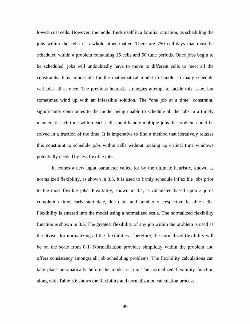
lowest cost cells. However, the model finds itself in a familiar situation, as scheduling the
jobs within the cells is a whole other matter. There are 750 cell-days that must be
scheduled within a problem containing 15 cells and 50 time periods. Once jobs begin to
be scheduled, jobs will undoubtedly have to move to different cells to meet all the
constraints. It is impossible for the mathematical model to handle so many schedule
variables all at once. The previous heuristic strategies attempt to tackle this issue, but
sometimes wind up with an infeasible solution. The “one job at a time” constraint,
significantly contributes to the model being unable to schedule all the jobs in a timely
manner. If each time within each cell, could handle multiple jobs the problem could be
solved in a fraction of the time. It is imperative to find a method that iteratively relaxes
this constraint to schedule jobs within cells without locking up critical time windows
potentially needed by less flexible jobs.
In comes a new input parameter called for by the ultimate heuristic, known as
normalized flexibility, as shown in 3.3. It is used to firmly schedule inflexible jobs prior
to the most flexible jobs. Flexibility, shown in 3.4, is calculated based upon a job’s
completion time, early start date, due date, and number of respective feasible cells.
Flexibility is entered into the model using a normalized scale. The normalized flexibility
function is shown in 3.5. The greatest flexibility of any job within the problem is used as
the divisor for normalizing all the flexibilities. Therefore, the normalized flexibility will
be on the scale from 0-1. Normalization provides simplicity within the problem and
offers consistency amongst all job scheduling problems. The flexibility calculations can
take place automatically before the model is run. The normalized flexibility function
along with Table 3.6 shows the flexibility and normalization calculation process.
49
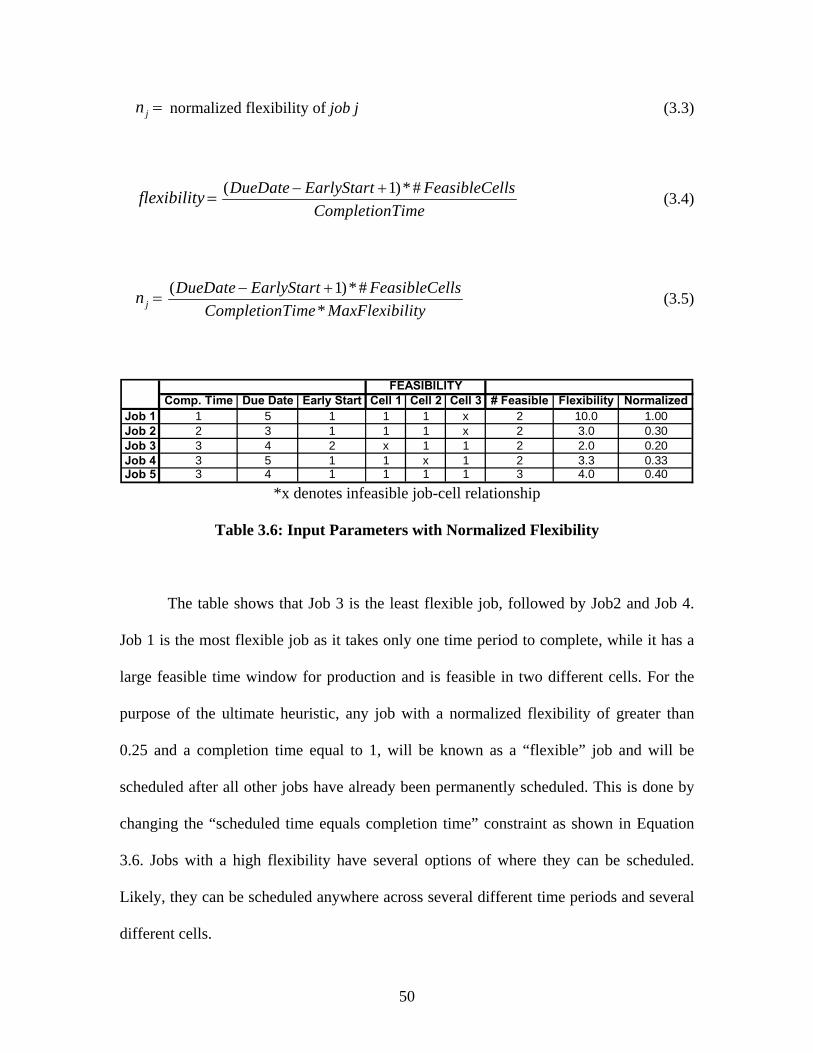
jn = normalized flexibility of job j (3.3)
flexibility = ( 1)*#DueDate EarlyStart FeasibleCellsCompletionTime
− + (3.4)
jn = ( 1)*#*
DueDate EarlyStart FeasibleCellsCompletionTime MaxFlexibility
− + (3.5)
Comp. Time Due Date Early Start Cell 1 Cell 2 Cell 3 # Feasible Flexibility NormalizedJob 1 1 5 1 1 1 x 2 10.0 1.00Job 2 2 3 1 1 1 x 2 3.0 0.30Job 3 3 4 2 x 1 1 2 2.0 0.20Job 4 3 5 1 1 x 1 2 3.3 0.33Job 5 3 4 1 1 1 1 3 4.0 0.40
FEASIBILITY
*x denotes infeasible job-cell relationship
Table 3.6: Input Parameters with Normalized Flexibility
The table shows that Job 3 is the least flexible job, followed by Job2 and Job 4.
Job 1 is the most flexible job as it takes only one time period to complete, while it has a
large feasible time window for production and is feasible in two different cells. For the
purpose of the ultimate heuristic, any job with a normalized flexibility of greater than
0.25 and a completion time equal to 1, will be known as a “flexible” job and will be
scheduled after all other jobs have already been permanently scheduled. This is done by
changing the “scheduled time equals completion time” constraint as shown in Equation
3.6. Jobs with a high flexibility have several options of where they can be scheduled.
Likely, they can be scheduled anywhere across several different time periods and several
different cells.
50
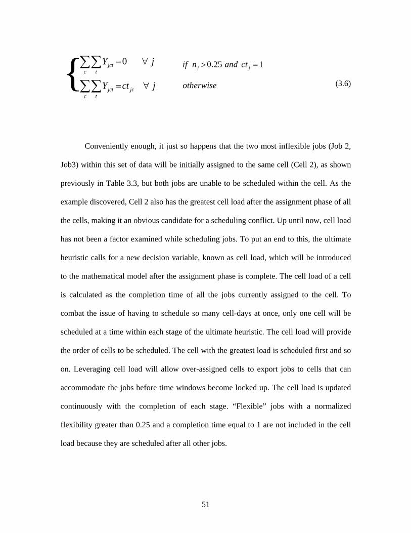
0.25 1j jif n and ct> =
jct jcc t
Y ct j= ∀∑∑ otherwise
0jctc t
Y j= ∀∑∑{ (3.6) Conveniently enough, it just so happens that the two most inflexible jobs (Job 2,
Job3) within this set of data will be initially assigned to the same cell (Cell 2), as shown
previously in Table 3.3, but both jobs are unable to be scheduled within the cell. As the
example discovered, Cell 2 also has the greatest cell load after the assignment phase of all
the cells, making it an obvious candidate for a scheduling conflict. Up until now, cell load
has not been a factor examined while scheduling jobs. To put an end to this, the ultimate
heuristic calls for a new decision variable, known as cell load, which will be introduced
to the mathematical model after the assignment phase is complete. The cell load of a cell
is calculated as the completion time of all the jobs currently assigned to the cell. To
combat the issue of having to schedule so many cell-days at once, only one cell will be
scheduled at a time within each stage of the ultimate heuristic. The cell load will provide
the order of cells to be scheduled. The cell with the greatest load is scheduled first and so
on. Leveraging cell load will allow over-assigned cells to export jobs to cells that can
accommodate the jobs before time windows become locked up. The cell load is updated
continuously with the completion of each stage. “Flexible” jobs with a normalized
flexibility greater than 0.25 and a completion time equal to 1 are not included in the cell
load because they are scheduled after all other jobs. 51
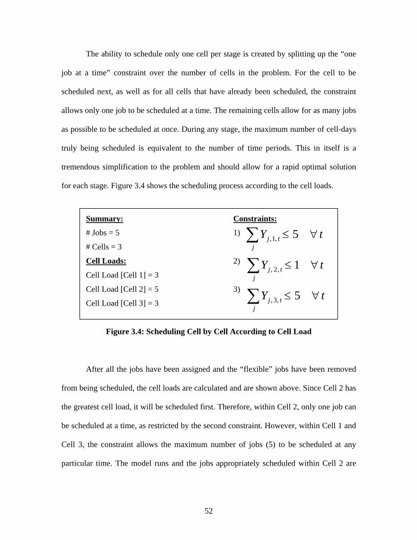
The ability to schedule only one cell per stage is created by splitting up the “one
job at a time” constraint over the number of cells in the problem. For the cell to be
scheduled next, as well as for all cells that have already been scheduled, the constraint
allows only one job to be scheduled at a time. The remaining cells allow for as many jobs
as possible to be scheduled at once. During any stage, the maximum number of cell-days
truly being scheduled is equivalent to the number of time periods. This in itself is a
tremendous simplification to the problem and should allow for a rapid optimal solution
for each stage. Figure 3.4 shows the scheduling process according to the cell loads.
Summary: Constraints:
# Jobs = 5 1) tYj
tj ∀≤∑ 5,1,# Cells = 3
Cell Loads: 2) tYj
tj ∀≤∑Cell Load [Cell 1] = 3
Cell Load [Cell 2] = 5 3)
Cell Load [Cell 3] = 3
1,2,
tYj
tj ∀≤∑ 5,3,
Figure 3.4: Scheduling Cell by Cell According to Cell Load
After all the jobs have been assigned and the “flexible” jobs have been removed
from being scheduled, the cell loads are calculated and are shown above. Since Cell 2 has
the greatest cell load, it will be scheduled first. Therefore, within Cell 2, only one job can
be scheduled at a time, as restricted by the second constraint. However, within Cell 1 and
Cell 3, the constraint allows the maximum number of jobs (5) to be scheduled at any
particular time. The model runs and the jobs appropriately scheduled within Cell 2 are
52
permanently scheduled. The jobs that are not correctly scheduled are reassigned to the
next best cell and the process continues with the cell with the next greatest load.
Figure 3.5 shows the flow diagram for the ultimate heuristic. The ultimate
heuristic uses a greedy multi-phase iterative process to first assign jobs to particular cells
and then to schedule the jobs within the assigned cells. The heuristic relaxes several
variables and constraints along the way, while taking into account the flexibility of the
different jobs and the current load of the different cells.
53

Run Model
Stage 1:Assign most jobs to only one cell
1. Relax integrality on assignment variable.2. Relax integrality on schedule variable.
Stage 2:Assign remaining jobs
to only one cell
1. If job is assigned to only one cell, transform job-to-cell assignment variable into constraints.2. Change assignment variable back to integer form.
Are all assignments
integer?
Stage 4...n:Schedule remaining cell with greatest cell load
1. For cell to be scheduled and all previously scheduled cells, allow only one job to be scheduled at one time.2. For all remaining cells, allow the maximum number of jobs to be scheduled at one time.
Heuristic Feasible Solution
Stage 3:Calculate cell loads
1. Add all job-to-cell assignment variables to the model as constraints. 2. Change constraint to not schedule “flexible” jobs.3. Add cell load variable and constraint to the model.
NO
Run Model
Run Model
Run Model
Run Model
1. Transform all schedule variables for current cell into constraints and add to the model.
≤ 20% cells not
scheduled?
YES
NO
1. If a job is assigned to two cells, one of which has already been scheduled, disallow assignment to the current cell only.2. If a job is assigned to multiple cells, change the assignment variable to the lowest value new cell that has not been scheduled yet and disallow assignment to the current cell.3. With the exception of the job(s) assigned to multiple cells, transform all schedule variables for current cell into constraints and add to the model.
Any newly assigned
cells already scheduled?
Stage n+1:Schedule remaining cells
and “flexible” jobs
1. For all cells, allow only one job to be scheduled at one time2. Change constraint to schedule “flexible” jobs.3. Eliminate all assignment variables added from stage 1 and stage 2.4. Change assignment variable back to integer form.
NO
Stage 0:Adjust mathematical model to
accommodate heuristic
1. Compute normalized flexibility input parameter.2. Split up “one job at a time” constraint for each cell.3. Adjust “schedule time equals completion time” constraint to accommodate “flexible” jobs
YES
YES
1. Relax integrality on assignment variable.2. Change schedule variable back to integer form.3. Change constraint to allow for multiple cell assignments.
Figure 3.5: Ultimate Heuristic
Several of the techniques present within this heuristic have already been partially
explained. To best describe the heuristic in its entirety and to illustrate the dynamics of
the whole procedure, the same simple problem will be used, but the heuristic will be
applied. Table 3.7 shows the input parameters for the problem.
54

Comp. Time Due Date Early Start Cell 1 Cell2 Cell3 Cell 1 Cell 2 Cell 3 # Feasible Flexibility NormalizedJob 1 1 5 1 2 4 x 1 1 x 2 10.0 1.00Job 2 2 3 1 2 1 x 1 1 x 2 3.0 0.30Job 3 3 4 2 x 1 4 x 1 1 2 2.0 0.20Job 4 3 5 1 2 x 5 1 x 1 2 3.3 0.33Job 5 3 4 1 3 5 1 1 1 1 3 4.0 0.40
FEASIBILITYCOST
*x denotes infeasible job-cell relationship
Table 3.7: Input Parameters with Normalized Flexibility
The following is the state of the OPL model and the OPL data after stage 0 is
complete. The grayed contents are additions or changes made to the baseline
mathematical model to accommodate the heuristic. A double backslash (//) denotes a
comment within the programming code and therefore the entire following line is not
actually used in the model.
OPL Model:
Notation:
int nbCell = ...; range Cell 1..nbCell; int nbTime = ...; range Time 1..nbTime; int nbJob = ...; range Job 1..nbJob; Input Parameters: float+ feasible[Job,Cell]=...; float+ completionTime[Job]=...; float+ earlyStart[Job]=...; float+ dueDate[Job]=...; float+ cost[Job,Cell]=...; float+ flexibility[Job]=...;
55

Decision Variables: var int+ assignment[Job,Cell] in 0..1; var int+ schedule[Job,Cell,Time] in 0..1; var float+ start[Job] in 1..nbTime; var float+ finish[Job] in 1..nbTime; //var float+ cellLoad[Cell] in 1..nbTime; Objective Function: minimize sum(j in Job, c in Cell) (assignment[j,c] * cost[j,c] * completionTime[j]) Constraints: subject to { //one cell only forall (j in Job) sum (c in Cell) assignment[j,c] = 1; //cell feasibility forall (j in Job & c in Cell) assignment[j,c]<=feasible[j,c]; //schedule only if assigned forall (j in Job, c in Cell) sum (t in Time) schedule[j,c,t] <= nbTime * assignment[j,c]; //one job at a time forall (t in Time) sum (j in Job) schedule[j,1,t] <= 1; forall (t in Time) sum (j in Job) schedule[j,2,t] <= 1; forall (t in Time) sum (j in Job) schedule[j,3,t] <= 1;
56
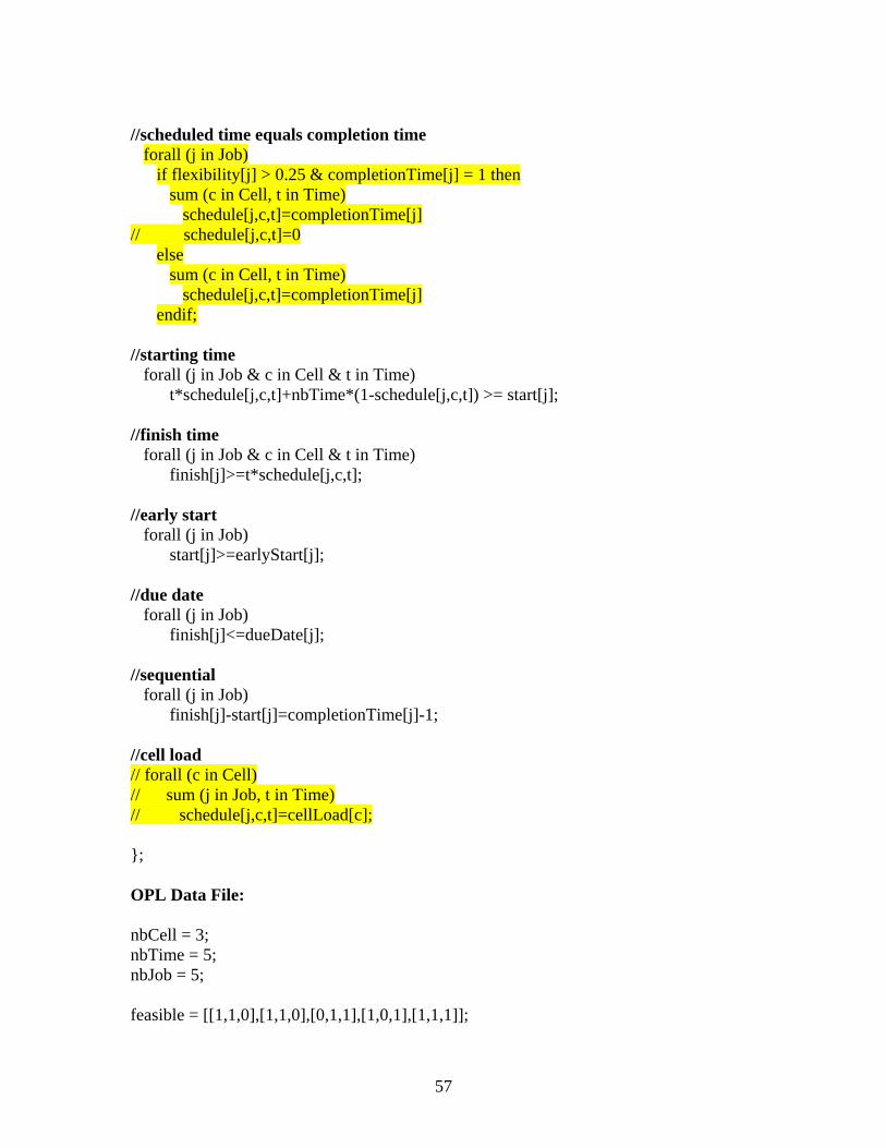
//scheduled time equals completion time forall (j in Job) if flexibility[j] > 0.25 & completionTime[j] = 1 then sum (c in Cell, t in Time) schedule[j,c,t]=completionTime[j] // schedule[j,c,t]=0 else sum (c in Cell, t in Time) schedule[j,c,t]=completionTime[j] endif; //starting time forall (j in Job & c in Cell & t in Time) t*schedule[j,c,t]+nbTime*(1-schedule[j,c,t]) >= start[j]; //finish time forall (j in Job & c in Cell & t in Time) finish[j]>=t*schedule[j,c,t]; //early start forall (j in Job) start[j]>=earlyStart[j]; //due date forall (j in Job) finish[j]<=dueDate[j]; //sequential forall (j in Job) finish[j]-start[j]=completionTime[j]-1; //cell load // forall (c in Cell) // sum (j in Job, t in Time) // schedule[j,c,t]=cellLoad[c]; }; OPL Data File: nbCell = 3; nbTime = 5; nbJob = 5; feasible = [[1,1,0],[1,1,0],[0,1,1],[1,0,1],[1,1,1]];
57

completionTime = [1,2,3,3,3]; earlyStart = [1,1,2,1,1]; dueDate = [5,3,4,5,4]; cost = [[2,4,0],[2,1,0],[0,1,4],[2,0,5],[1,5,1]]; flexibililty = [1.00,0.30,0.20,0.33,0.40]; During stage 0, the flexibility input parameter is added to the model and the
normalized flexibility values for each job are added into the data file. The cell load
variable and constraint is present in the model, but are commented out until stage 3, when
they are needed. The same can be said for the constraint that does not schedule “flexible”
jobs. Finally, as a whole, the “one job at a time” constraint is unchanged. However, it has
been split up over the three cells for ease of use starting at stage 4.
Modified Variables for Stage 1: var float+ assignment[Job,Cell] in 0..1; var float+ schedule[Job,Cell,Time] in 0..1;
In stage 1, both the integrality on the assignment variable and the schedule
variable is relaxed, in an attempt to assign as many jobs as possible in a short
computation time. The model is run and the assignment variable results are shown below.
Variable Results from Stage 1: (assigning initial jobs) assignment[1,1] = 1.0000 assignment[2,2] = 1.0000 assignment[3,2] = 1.0000 assignment[4,1] = 1.0000 assignment[5,1] = 0.6000 assignment[5,3] = 0.4000 New Constraints for Stage 2: assignment[1,1] = 1; assignment[2,2] = 1;
58
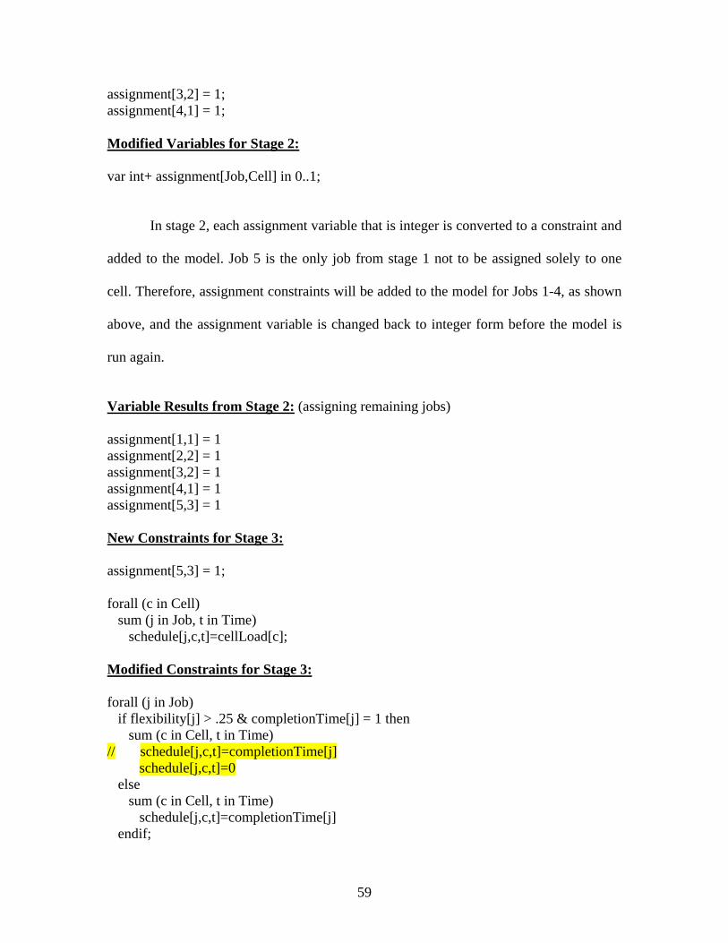
assignment[3,2] = 1; assignment[4,1] = 1; Modified Variables for Stage 2: var int+ assignment[Job,Cell] in 0..1;
In stage 2, each assignment variable that is integer is converted to a constraint and
added to the model. Job 5 is the only job from stage 1 not to be assigned solely to one
cell. Therefore, assignment constraints will be added to the model for Jobs 1-4, as shown
above, and the assignment variable is changed back to integer form before the model is
run again.
Variable Results from Stage 2: (assigning remaining jobs) assignment[1,1] = 1 assignment[2,2] = 1 assignment[3,2] = 1 assignment[4,1] = 1 assignment[5,3] = 1 New Constraints for Stage 3: assignment[5,3] = 1; forall (c in Cell) sum (j in Job, t in Time) schedule[j,c,t]=cellLoad[c]; Modified Constraints for Stage 3: forall (j in Job) if flexibility[j] > .25 & completionTime[j] = 1 then sum (c in Cell, t in Time) // schedule[j,c,t]=completionTime[j] schedule[j,c,t]=0 else sum (c in Cell, t in Time) schedule[j,c,t]=completionTime[j] endif;
59

New Variables for Stage 3: var float+ cellLoad[Cell] in 1..nbTime; Heading into stage 3, all jobs have been distinctly assigned to one cell, with Job 5
being constrained to Cell 3. The goal of stage 3 is to determine cell loads for each cell in
order to provide the cell scheduling order. Therefore, the cell load variable and constraint
are added to the model. This is its own stage for two main reasons. First, it takes
significantly longer to determine the cell load when all jobs are not already assigned to
one cell only. Secondly, the jobs that are “flexible” (flexibility > 0.25 and completion
time = 1), can be removed from the cell load, by the slight modification to the constraint
just shown. The commented line is removed and the line directly below is added to the
model. “Flexible” jobs are still assigned to a cell to provide time gaps that offer added
elasticity to the jobs that are scheduled first. The model is ready to be run again.
Variable Results from Stage 3: (calculating cell loads) cellLoad[1] = 3.0000 cellLoad[2] = 5.0000 cellLoad[3] = 3.0000 Modified Constraints for Stage 4: forall (t in Time) sum (j in Job) schedule[j,1,t] <= nbJob; forall (t in Time) sum (j in Job) schedule[j,2,t] <= 1;
60
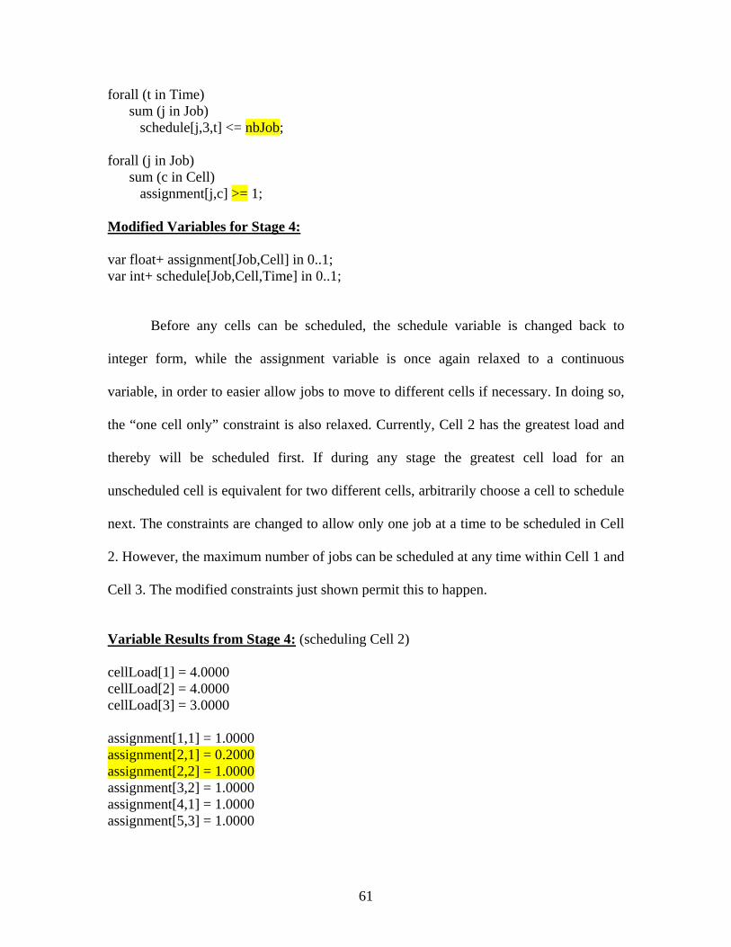
forall (t in Time) sum (j in Job) schedule[j,3,t] <= nbJob; forall (j in Job) sum (c in Cell) assignment[j,c] >= 1; Modified Variables for Stage 4: var float+ assignment[Job,Cell] in 0..1; var int+ schedule[Job,Cell,Time] in 0..1; Before any cells can be scheduled, the schedule variable is changed back to
integer form, while the assignment variable is once again relaxed to a continuous
variable, in order to easier allow jobs to move to different cells if necessary. In doing so,
the “one cell only” constraint is also relaxed. Currently, Cell 2 has the greatest load and
thereby will be scheduled first. If during any stage the greatest cell load for an
unscheduled cell is equivalent for two different cells, arbitrarily choose a cell to schedule
next. The constraints are changed to allow only one job at a time to be scheduled in Cell
2. However, the maximum number of jobs can be scheduled at any time within Cell 1 and
Cell 3. The modified constraints just shown permit this to happen.
Variable Results from Stage 4: (scheduling Cell 2) cellLoad[1] = 4.0000 cellLoad[2] = 4.0000 cellLoad[3] = 3.0000 assignment[1,1] = 1.0000 assignment[2,1] = 0.2000 assignment[2,2] = 1.0000 assignment[3,2] = 1.0000 assignment[4,1] = 1.0000 assignment[5,3] = 1.0000
61

schedule[2,1,2] = 1 schedule[4,1,1] = 1 schedule[4,1,2] = 1 schedule[4,1,3] = 1 schedule[2,2,1] = 1 schedule[3,2,2] = 1 schedule[3,2,3] = 1 schedule[3,2,4] = 1 schedule[5,3,1] = 1 schedule[5,3,2] = 1 schedule[5,3,3] = 1 New Constraints for Stage 5: assignment[2,1] = 1; schedule[3,2,2] = 1; schedule[3,2,3] = 1; schedule[3,2,4] = 1; Modified Constraints for Stage 5: assignment[2,2] = 0; forall (t in Time) sum (j in Job) schedule[j,1,t] <= 1;
The grayed variables from stage 4 show that Job 2 gets assigned to two different
cells and thus winds up getting scheduled across the two cells. Consequently, the
assignment variable constraint is changed to assign Job 2 to Cell 1, the next best cell
option cost-wise. If a job is assigned to multiple other un-scheduled cells with an
equivalent variable value, constrain the job to the cell with the smallest cell load. Another
assignment variable constraint is added to disallow Job 2 to be assigned to Cell 2 again. If
62

Cell 1 had already been scheduled, simply disallow scheduling to Cell 2, without forcing
the job to Cell 1. This occurs because it is likely that Cell 1, since it had already been
scheduled, will not have room for another job. To avoid changing the assignment again
after the next stage, this modified action is taken. The remaining jobs scheduled in Cell 2,
not assigned to multiple cells, now become permanently scheduled through use of the
schedule variable constraints. Notice that Job 1 was not scheduled anywhere because it is
a “flexible” job. Since Cell 1 has the greatest cell load of the jobs not yet scheduled, it
will be scheduled next and so the “one job at a time” constraint is applied for Cell 1. The
current state of the schedule, after Stage 4 and before Stage 5, is shown in Table 3.8.
1 2 3 4 5Cell 1Cell 2 Job3 Job3 Job3Cell 3
TIME
Table 3.8: State of Schedule after Stage 4
Variable Results from Stage 5: (scheduling Cell 1) cellLoad[1] = 5.0000 cellLoad[2] = 3.0000 cellLoad[3] = 3.0000 assignment[1,1] = 1.0000 assignment[2,1] = 1.0000 assignment[3,2] = 1.0000 assignment[4,1] = 1.0000 assignment[5,3] = 1.0000 schedule[2,1,1] = 1 schedule[2,1,2] = 1 schedule[4,1,3] = 1 schedule[4,1,4] = 1 schedule[4,1,5] = 1
63
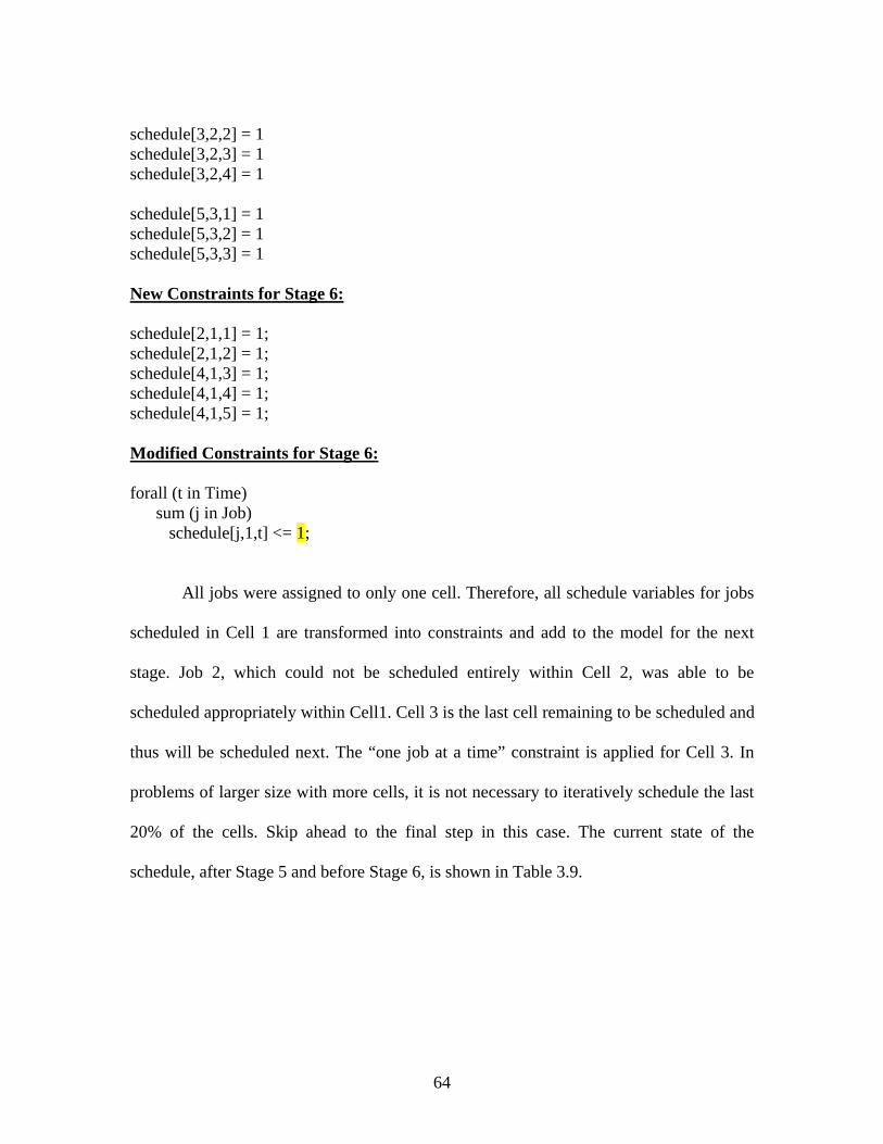
schedule[3,2,2] = 1 schedule[3,2,3] = 1 schedule[3,2,4] = 1 schedule[5,3,1] = 1 schedule[5,3,2] = 1 schedule[5,3,3] = 1 New Constraints for Stage 6: schedule[2,1,1] = 1; schedule[2,1,2] = 1; schedule[4,1,3] = 1; schedule[4,1,4] = 1; schedule[4,1,5] = 1; Modified Constraints for Stage 6: forall (t in Time) sum (j in Job) schedule[j,1,t] <= 1;
All jobs were assigned to only one cell. Therefore, all schedule variables for jobs
scheduled in Cell 1 are transformed into constraints and add to the model for the next
stage. Job 2, which could not be scheduled entirely within Cell 2, was able to be
scheduled appropriately within Cell1. Cell 3 is the last cell remaining to be scheduled and
thus will be scheduled next. The “one job at a time” constraint is applied for Cell 3. In
problems of larger size with more cells, it is not necessary to iteratively schedule the last
20% of the cells. Skip ahead to the final step in this case. The current state of the
schedule, after Stage 5 and before Stage 6, is shown in Table 3.9.
64
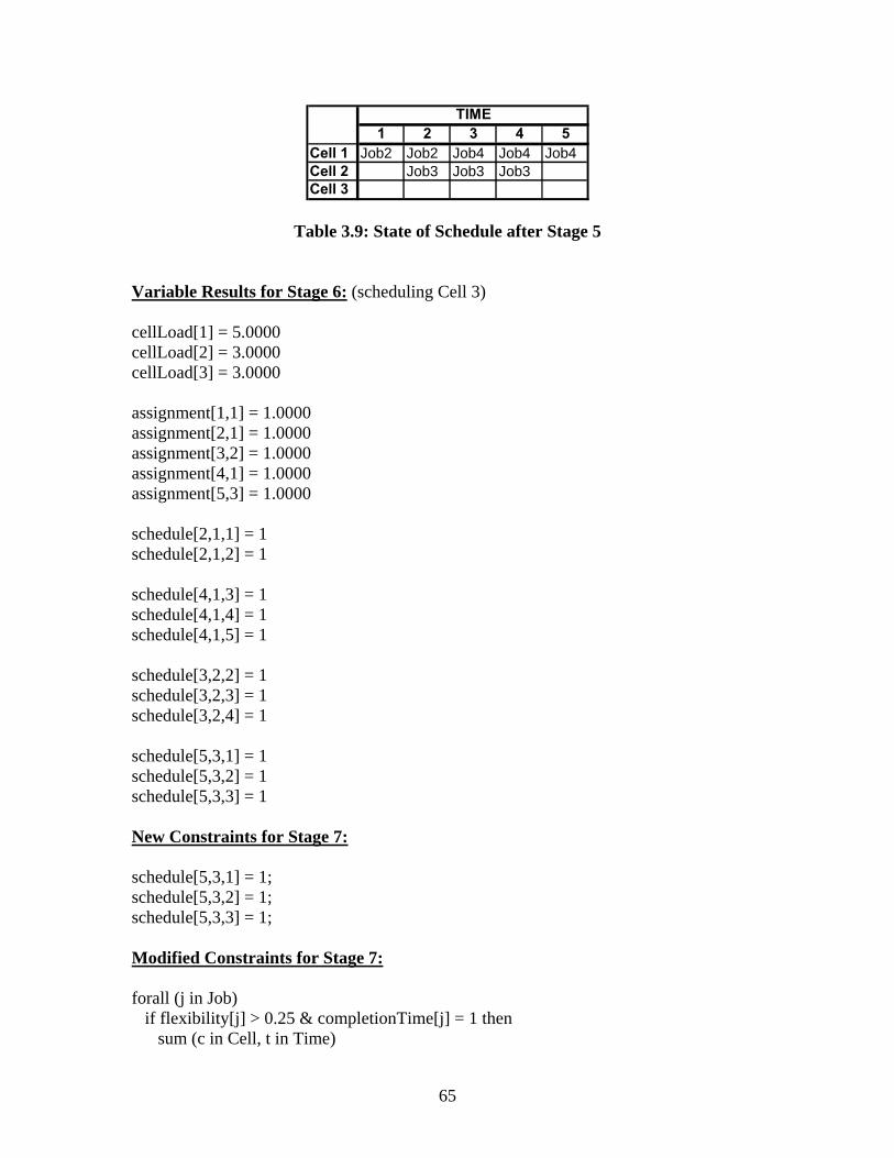
1 2 3 4 5Cell 1 Job2 Job2 Job4 Job4 Job4Cell 2 Job3 Job3 Job3Cell 3
TIME
Table 3.9: State of Schedule after Stage 5
Variable Results for Stage 6: (scheduling Cell 3) cellLoad[1] = 5.0000 cellLoad[2] = 3.0000 cellLoad[3] = 3.0000 assignment[1,1] = 1.0000 assignment[2,1] = 1.0000 assignment[3,2] = 1.0000 assignment[4,1] = 1.0000 assignment[5,3] = 1.0000 schedule[2,1,1] = 1 schedule[2,1,2] = 1 schedule[4,1,3] = 1 schedule[4,1,4] = 1 schedule[4,1,5] = 1 schedule[3,2,2] = 1 schedule[3,2,3] = 1 schedule[3,2,4] = 1 schedule[5,3,1] = 1 schedule[5,3,2] = 1 schedule[5,3,3] = 1 New Constraints for Stage 7: schedule[5,3,1] = 1; schedule[5,3,2] = 1; schedule[5,3,3] = 1; Modified Constraints for Stage 7: forall (j in Job) if flexibility[j] > 0.25 & completionTime[j] = 1 then sum (c in Cell, t in Time)
65
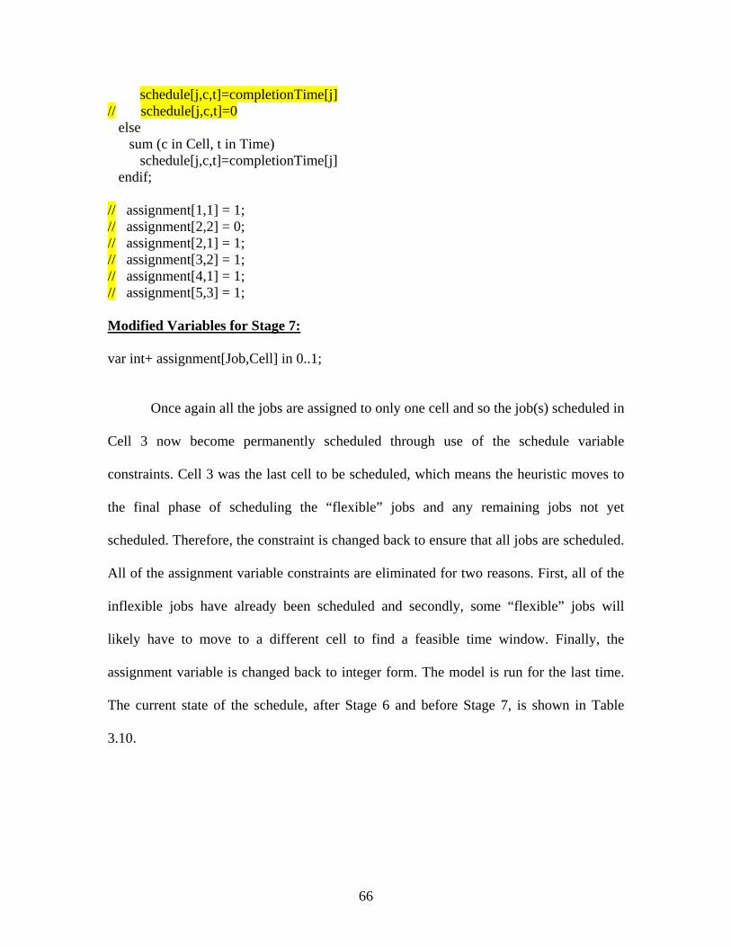
schedule[j,c,t]=completionTime[j] // schedule[j,c,t]=0 else sum (c in Cell, t in Time) schedule[j,c,t]=completionTime[j] endif; // assignment[1,1] = 1; // assignment[2,2] = 0; // assignment[2,1] = 1; // assignment[3,2] = 1; // assignment[4,1] = 1; // assignment[5,3] = 1; Modified Variables for Stage 7: var int+ assignment[Job,Cell] in 0..1; Once again all the jobs are assigned to only one cell and so the job(s) scheduled in
Cell 3 now become permanently scheduled through use of the schedule variable
constraints. Cell 3 was the last cell to be scheduled, which means the heuristic moves to
the final phase of scheduling the “flexible” jobs and any remaining jobs not yet
scheduled. Therefore, the constraint is changed back to ensure that all jobs are scheduled.
All of the assignment variable constraints are eliminated for two reasons. First, all of the
inflexible jobs have already been scheduled and secondly, some “flexible” jobs will
likely have to move to a different cell to find a feasible time window. Finally, the
assignment variable is changed back to integer form. The model is run for the last time.
The current state of the schedule, after Stage 6 and before Stage 7, is shown in Table
3.10.
66
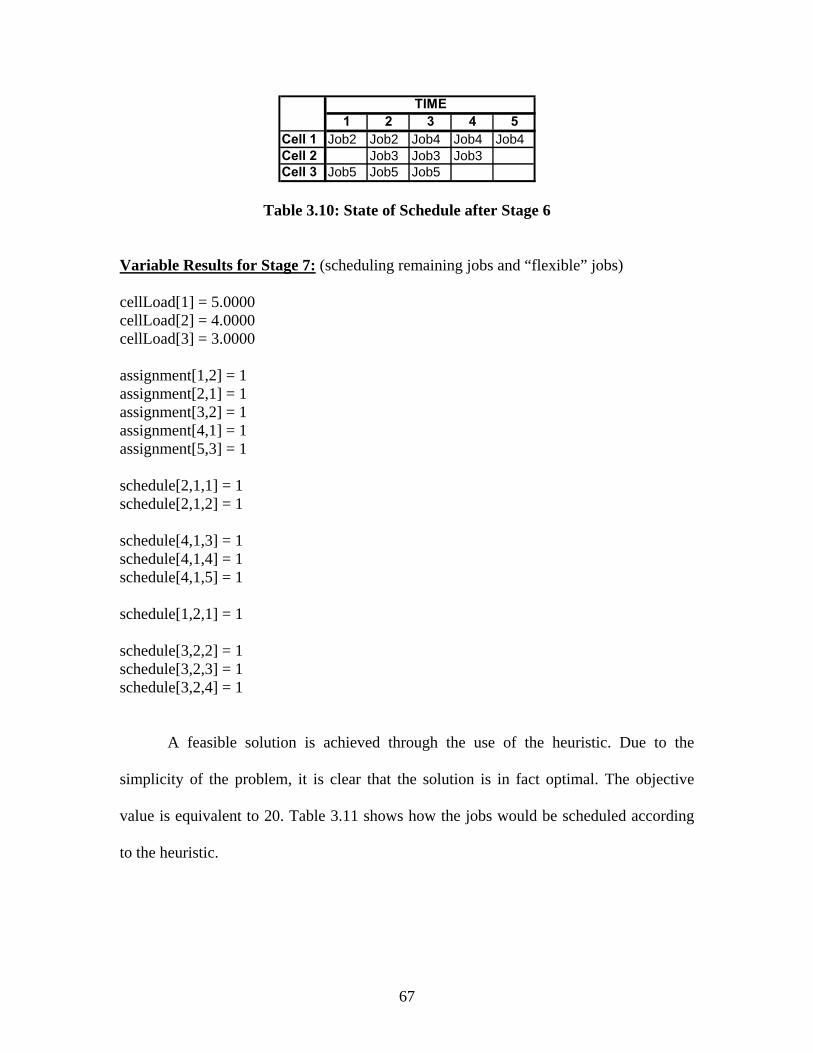
1 2 3 4 5Cell 1 Job2 Job2 Job4 Job4 Job4Cell 2 Job3 Job3 Job3Cell 3 Job5 Job5 Job5
TIME
Table 3.10: State of Schedule after Stage 6
Variable Results for Stage 7: (scheduling remaining jobs and “flexible” jobs) cellLoad[1] = 5.0000 cellLoad[2] = 4.0000 cellLoad[3] = 3.0000 assignment[1,2] = 1 assignment[2,1] = 1 assignment[3,2] = 1 assignment[4,1] = 1 assignment[5,3] = 1 schedule[2,1,1] = 1 schedule[2,1,2] = 1 schedule[4,1,3] = 1 schedule[4,1,4] = 1 schedule[4,1,5] = 1 schedule[1,2,1] = 1 schedule[3,2,2] = 1 schedule[3,2,3] = 1 schedule[3,2,4] = 1 A feasible solution is achieved through the use of the heuristic. Due to the
simplicity of the problem, it is clear that the solution is in fact optimal. The objective
value is equivalent to 20. Table 3.11 shows how the jobs would be scheduled according
to the heuristic.
67

1 2 3 4 5Cell 1 Job2 Job2 Job4 Job4 Job4Cell 2 Job1 Job3 Job3 Job3Cell 3 Job5 Job5 Job5
TIME
Table 3.11: Heuristic Feasible Solution Schedule
3.5.4 Summary
The ultimate heuristic takes advantage of several techniques to arrive at a near
optimal solution in a practical amount of solving time. The separation of the assignment
process and schedule process allows the overall schedule to be broken down into two
logical phases. Once the jobs are assigned to cells, the iterative scheduling phase is able
to begin. Postponing the scheduling of “flexible” jobs and scheduling the greatest load
cells first, limit the number of cell-days that must be scheduled at one time, while
allowing ample space for the movement of jobs to different cells or time periods, before
locking other jobs into specific positions. This vastly improves the feasibility chances of
the final heuristic solution, especially on larger problems.
To further improve the solving time of the problem using the heuristic, a time
limit could be placed on each stage. At times, the solver gets stuck in one stage for an
extended period of time with a very slight opportunity for improvement. A time limit
would stop the solver and proceed with the best feasible solution. Likely, the overall
solution will not be as good, but if timing is an important factor, this could be a direction
to consider.
To additionally aid to the efficiency of the heuristic, it is beneficial to assign
different costs to each feasible cell for a particular job. For example, if it is equally cost
effective to produce Job 1 in Cell 1 and Cell2, the cost input parameter would be the
68
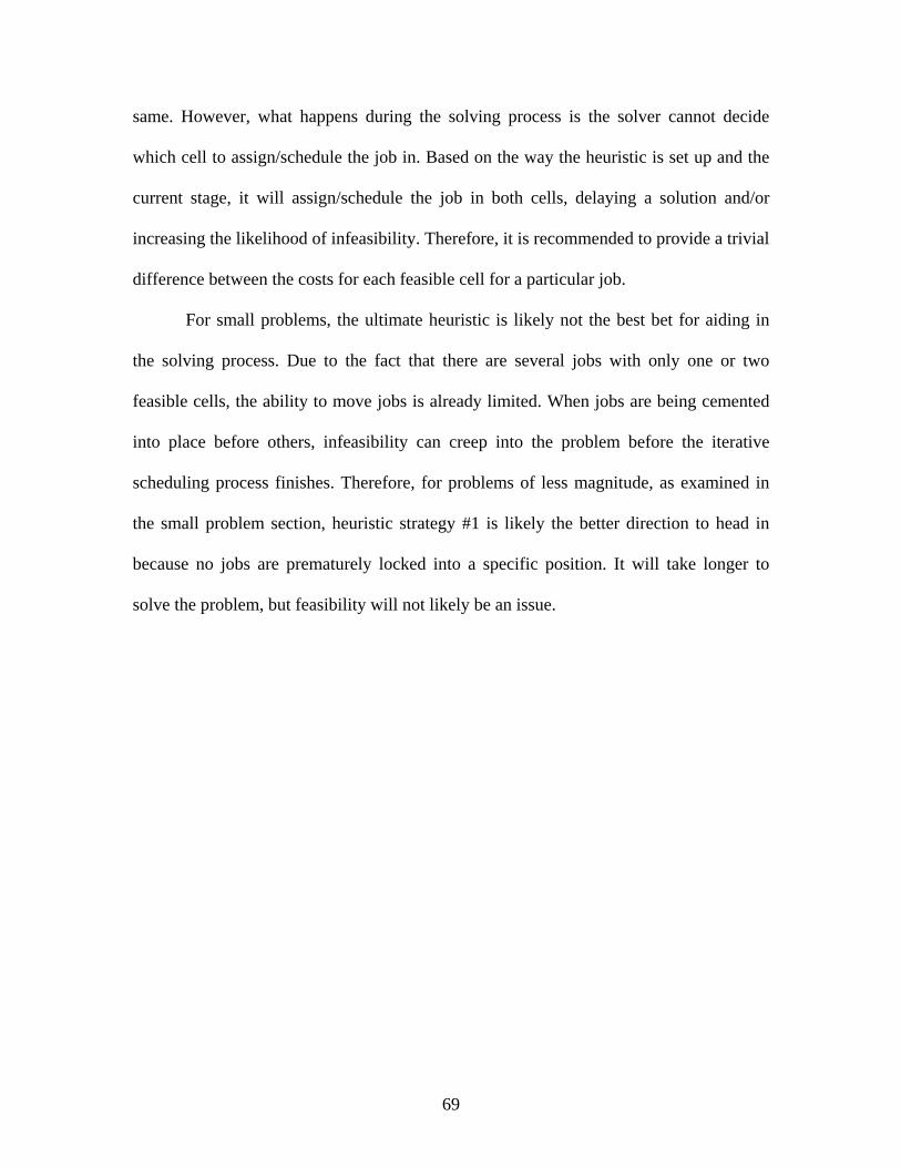
same. However, what happens during the solving process is the solver cannot decide
which cell to assign/schedule the job in. Based on the way the heuristic is set up and the
current stage, it will assign/schedule the job in both cells, delaying a solution and/or
increasing the likelihood of infeasibility. Therefore, it is recommended to provide a trivial
difference between the costs for each feasible cell for a particular job.
For small problems, the ultimate heuristic is likely not the best bet for aiding in
the solving process. Due to the fact that there are several jobs with only one or two
feasible cells, the ability to move jobs is already limited. When jobs are being cemented
into place before others, infeasibility can creep into the problem before the iterative
scheduling process finishes. Therefore, for problems of less magnitude, as examined in
the small problem section, heuristic strategy #1 is likely the better direction to head in
because no jobs are prematurely locked into a specific position. It will take longer to
solve the problem, but feasibility will not likely be an issue.
69

4 Results and Analysis
4.1 Small Problem Testing
Of the 30 small problems that were tested, only 16 problems could be solved
optimally within an hour. One hour was used as the measuring point for the sensible
purpose that a job schedule must be realized within a practical timeframe to be of
usefulness. An additional eight problems were able to render a feasible solution within
the one-hour window. The remaining problems went unsolved and thus the bound will be
used as the baseline value. The bound is not the optimal solution, but instead it is the best
possible solution. No solution can be better than the bound. Nevertheless, it is very likely
that the bound and the true optimal solution differ by some immeasurable amount. Each
of the 30 problems was also solved using the ultimate heuristic methods. Table 4.1 shows
the solution results for this set of problems.
For the first test, the heuristic solution is compared to the best possible solution.
In this case, it is either the optimal solution or the bound. If a problem has an optimal
solution, it is used. Otherwise, the bound is used. Each of the 30 problems is used within
this test. A one sample t-test is used to provide the analysis instead of a paired t-test, due
to the fact that the heuristic solution is impacted by the true value of the optimal solution.
For example, Problem A has an optimal solution of 100 and a heuristic solution of 105,
while Problem B has an optimal solution of 200 and a heuristic solution of 205. Both
heuristic solutions differ from their respective optimal solutions by 5, but problem B
actually has the better heuristic solution because the deviation is less from a percentage
standpoint. Problem A deviates by 5%, while problem B only deviates by 2.5%.
70
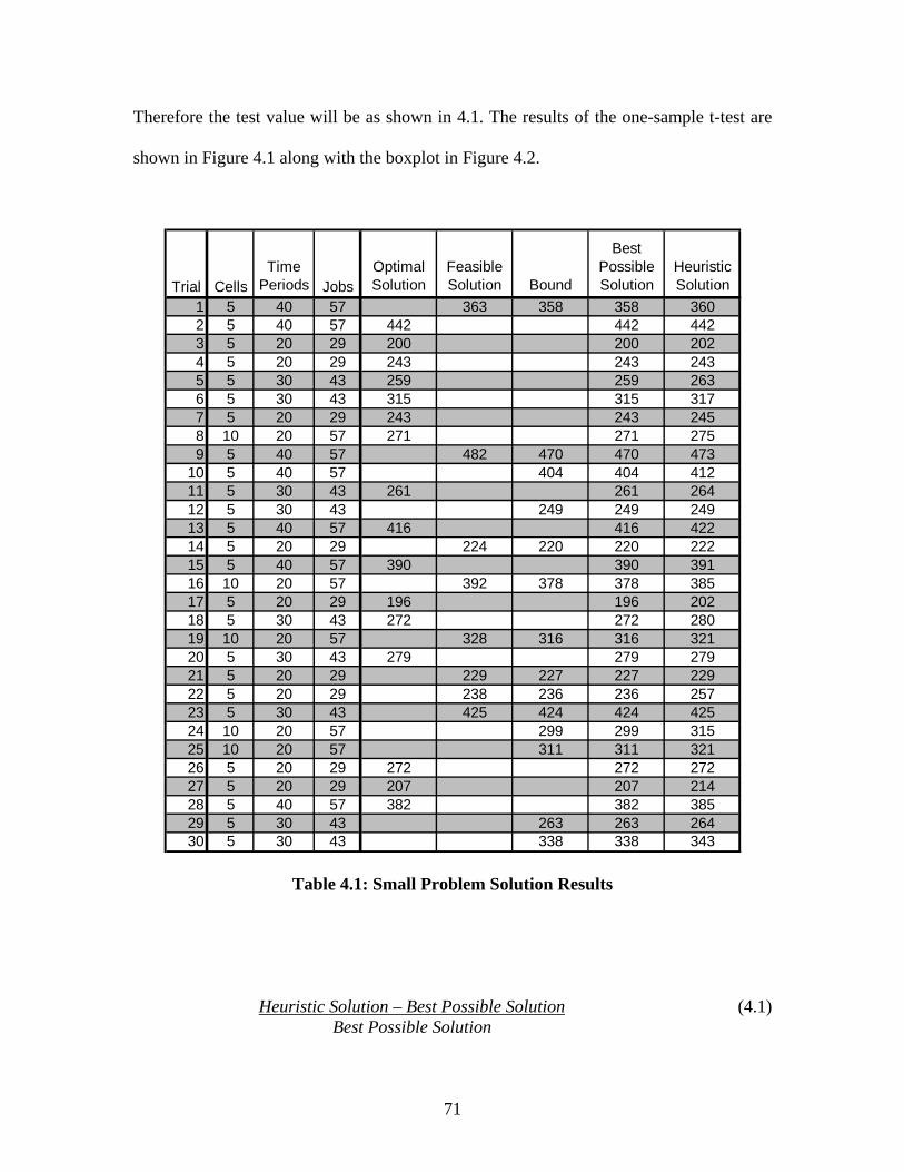
Therefore the test value will be as shown in 4.1. The results of the one-sample t-test are
shown in Figure 4.1 along with the boxplot in Figure 4.2.
Trial CellsTime
Periods JobsOptimal Solution
Feasible Solution Bound
Best Possible Solution
Heuristic Solution
1 5 40 57 363 358 358 3602 5 40 57 442 442 4423 5 20 29 200 200 2024 5 20 29 243 243 2435 5 30 43 259 259 2636 5 30 43 315 315 3177 5 20 29 243 243 2458 10 20 57 271 271 2759 5 40 57 482 470 470 473
10 5 40 57 404 404 41211 5 30 43 261 261 26412 5 30 43 249 249 24913 5 40 57 416 416 42214 5 20 29 224 220 220 22215 5 40 57 390 390 39116 10 20 57 392 378 378 38517 5 20 29 196 196 20218 5 30 43 272 272 28019 10 20 57 328 316 316 32120 5 30 43 279 279 27921 5 20 29 229 227 227 22922 5 20 29 238 236 236 25723 5 30 43 425 424 424 42524 10 20 57 299 299 31525 10 20 57 311 311 32126 5 20 29 272 272 27227 5 20 29 207 207 21428 5 40 57 382 382 38529 5 30 43 263 263 26430 5 30 43 338 338 343
Table 4.1: Small Problem Solution Results
Heuristic Solution – Best Possible Solution (4.1) Best Possible Solution
71

One-Sample T-Test: Deviation from Best Possible Solution Test of µ = 0 vs not = 0 Variable N Mean StDev SE Mean T P Deviation from Best 30 0.015485 0.018658 0.003406 4.55 0.000 95% Confidence Interval (0.008518, 0.022452)
Figure 4.1: One-Sample T-Test for Deviation from Best Possible Solution
Deviation from Best Possible Solution0.090.080.070.060.050.040.030.020.010.00
_X
Ho
Small Problem Boxplot of Deviation from Best Possible Solution(with Ho and 95% t-confidence interval for the mean)
Figure 4.2: Small Problem Boxplot of Deviation from Best Possible Solution
For the second test, only the problems that had an optimal solution were analyzed.
The heuristic solution is compared to the optimal solution. The test value for the 16
problems is as shown in 4.2. The results of the one-sample t-test are displayed in Figure
4.3.
72

Heuristic Solution – Optimal Solution (4.2) Optimal Solution
One-Sample T-Test: Deviation from Optimal Solution Test of µ = 0 vs not = 0 Variable N Mean StDev SE Mean T P Deviation from Optimal 16 0.011559 0.011197 0.002799 4.13 0.001 95% Confidence Interval (0.005592, 0.017525)
Figure 4.3: One-Sample T-Test for Deviation from Optimal Solution
The final test for this set looks only at problems that found a real solution.
Problems with an optimal solution or a feasible solution are used within the test. The
heuristic solution is compared to the optimal solution or feasible solution for each
problem. The test value is as shown in 4.3. The results of the one-sample t-test are
displayed in Figure 4.4.
Heuristic Solution – Real Solution (4.3) Real Solution
73

One-Sample T-Test: Deviation from Real Solution (Optimal or Feasible) Test of µ = 0 vs not = 0 Variable N Mean StDev SE Mean T P Deviation from Real 24 0.007905 0.021020 0.004291 1.84 0.078 95% Confidence Interval (-0.000971, 0.016781)
Figure 4.4: One-Sample T-Test for Deviation from Real Solution
Based upon the first test, there is a significant deviation between the heuristic
solution and the best possible solution. However, as the 95% confidence interval shows,
the deviation is not great. On average, the deviation is only 1.5%, with a 95% confidence
upper limit of 2.2%. The boxplot in Figure 4.2 shows that the majority of the problems
deviate by less than 2%, while a few problems with greater deviations are slightly
skewing the results. As the problems without an optimal solution are faded out, the
numbers improve. The second test shows that when an optimal solution was found, there
is still a slight deviation from the optimal solution with the heuristic solution. Again,
however, the difference is minimal, with an approximate mean of 1.1%. In the third test
as problems with feasible solutions are added, the deviation decreases once again. In fact,
more often than not, the heuristic solution is lower than the feasible solution. When the
best real solution is compared to the heuristic solution, with 95% confidence, there is not
a significant deviation between the heuristic solution and the real solution.
Though the heuristic solution may be slightly greater than the optimal solution,
the solving time that it takes to achieve the heuristic solution is substantially less than the
respective time for the optimal solution. Table 4.2 shows the computation time for each
74

heuristic solution, as well as the computation time for the optimal solutions, where
applicable.
TrialOptimal Solution
Solving Time (sec)Heuristic Solution
Solving Time (sec)1 92 248 123 50 24 7 25 695 126 21 87 13 18 63 79 1
10 2111 111 612 713 1591 1114 215 110 4916 1417 94 218 59 719 1220 1473 621 222 223 2624 1425 1126 79 227 18 128 798 829 1430 10
6
Table 4.2: Small Problem Solving Time Results
The following paired t-test in Figure 4.5 shows the significance of the difference
in solving time for the heuristic solution in comparison with the solving time for the
optimal solution. The 95% confidence interval shows that the true mean difference in
75

solving time is anywhere between approximately one minute and 10 minutes. Keep in
mind, that the results are based upon small problems. As the problems get larger, the
difference in solving time will becomes very difficult to measure, because the time to
solve optimally is so long.
Paired T-Test and Confidence Interval:
Optimal Solution Solving Time vs. Heuristic Solution Solving Time Paired T for Optimal Solution Solving Time - Heuristic Solution Solving Time N Mean StDev SE Mean Optimal Solution 16 339.375 522.173 130.543 Heuristic Soluti 16 8.500 11.460 2.865 Difference 16 330.875 521.602 130.401 95% Confidence Interval for mean difference: (52.933, 608.817) T-Test of mean difference = 0 (vs not = 0): T-Value = 2.54 P-Value = 0.023
Figure 4.5: Paired T-Test for Optimal Solving Time vs. Heuristic Solving Time
4.2 Medium Problem Testing
Fifteen problems were analyzed in the medium size class. However, only two
problems could even find a feasible solution, while none of the problems were able to
achieve an optimal solution even after running overnight or for several hours. Therefore,
from here on out, each heuristic solution will be compared against the respective bound
for the problem, with the test value being as shown in 4.4.
Heuristic Solution – Bound (4.4) Bound
76

Obviously, the deviation from the bound will be greater than or equal to the deviation
from the true optimal. Since the optimal solution is extremely difficult to solve for, the
bound will provide a conservative baseline to gauge the efficiency of the heuristic. The
results of the medium problems are shown in Table 4.3. The results of the one-sample t-
test are displayed in Figure 4.6.
Trial CellsTime
Periods JobsFeasible Solution Bound
Heuristic Solution
Heuristic Solving Time (sec)
1 5 50 71 502 508 622 5 50 71 503 516 513 15 20 85 309 312 244 15 20 85 307 325 845 15 20 85 258 263 326 15 20 85 307 308 367 10 30 85 426 426 508 10 30 85 560 561 539 5 50 71 459 469 75
10 10 30 85 473 473 3811 15 20 85 298 308 4512 5 50 71 567 573 3313 10 30 85 444 442 442 3714 10 30 85 396 405 5115 5 50 71 500 498 502 27
Table 4.3: Medium Problem Solution Results
One-Sample T-Test: Deviation from Bound Test of µ = 0 vs not = 0 Variable N Mean StDev SE Mean T P Deviation from Bound 15 0.015150 0.015998 0.004131 3.67 0.003 95% Confidence Interval (0.006291, 0.024009)
Figure 4.6: One-Sample T-Test for Deviation from Bound
77

Once again the t-test shows that when using 95% confidence, there is a significant
deviation of the heuristic solution from the bound. However, the deviation is obviously
very minimal, with the mean hovering around 1.5%. The heuristic solution’s deviation
from the true optimal solution is undoubtedly even lower. As Table 4.3 shows, the time to
solve heuristically is less than two minutes for each trial. Combining the slight deviation
with the minimal solving time, leads one to believe that the heuristic provides an efficient
procedure to solve problems of this size. The boxplot in Figure 4.7 shows that one
problem has a deviation of approximately 6%, but most of the remaining problems have a
deviation of less than 3%.
Deviation from Bound0.060.050.040.030.020.010.00
_X
Ho
Medium Problem Boxplot of Deviation from Bound(with Ho and 95% t-confidence interval for the mean)
Figure 4.7: Medium Problem Boxplot of Deviation from Bound
78
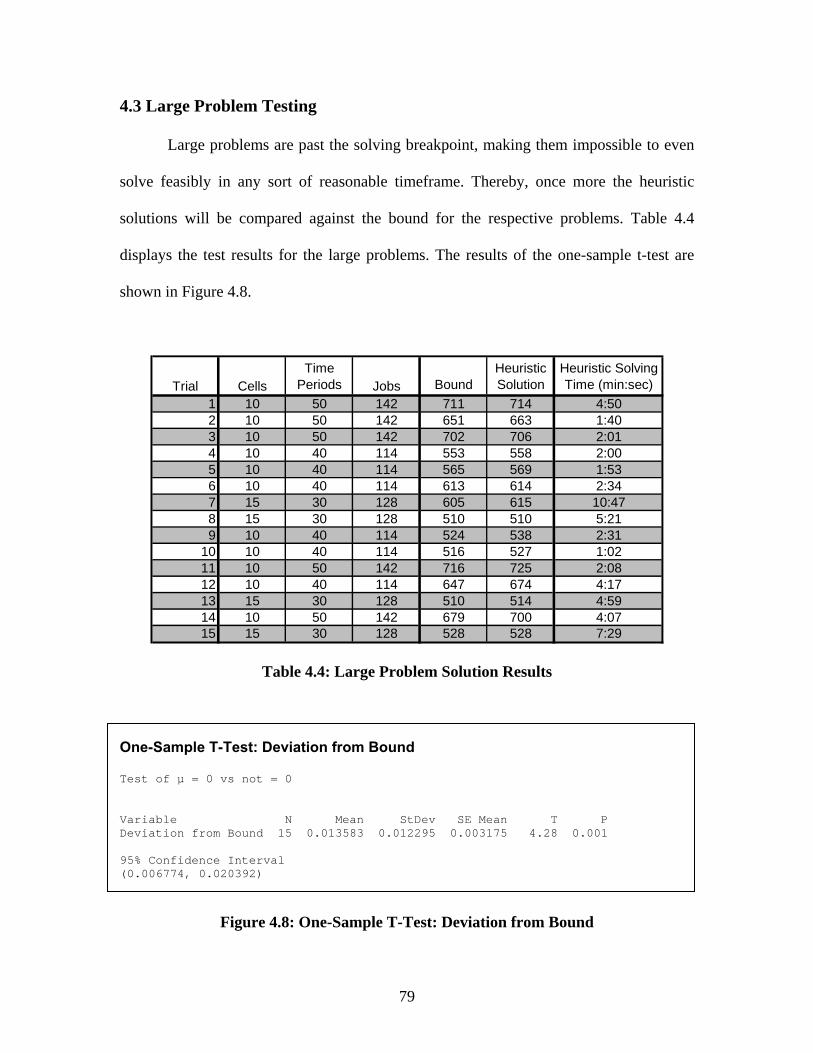
4.3 Large Problem Testing
Large problems are past the solving breakpoint, making them impossible to even
solve feasibly in any sort of reasonable timeframe. Thereby, once more the heuristic
solutions will be compared against the bound for the respective problems. Table 4.4
displays the test results for the large problems. The results of the one-sample t-test are
shown in Figure 4.8.
Trial CellsTime
Periods Jobs BoundHeuristic Solution
Heuristic Solving Time (min:sec)
1 10 50 142 711 714 4:502 10 50 142 651 663 1:403 10 50 142 702 706 2:014 10 40 114 553 558 2:005 10 40 114 565 569 1:536 10 40 114 613 614 2:347 15 30 128 605 615 10:478 15 30 128 510 510 5:219 10 40 114 524 538 2:31
10 10 40 114 516 527 1:0211 10 50 142 716 725 2:0812 10 40 114 647 674 4:1713 15 30 128 510 514 4:5914 10 50 142 679 700 4:0715 15 30 128 528 528 7:29
Table 4.4: Large Problem Solution Results
One-Sample T-Test: Deviation from Bound Test of µ = 0 vs not = 0 Variable N Mean StDev SE Mean T P Deviation from Bound 15 0.013583 0.012295 0.003175 4.28 0.001 95% Confidence Interval (0.006774, 0.020392)
Figure 4.8: One-Sample T-Test: Deviation from Bound
79

The t-test shows a significant deviation for the heuristic solution from the bound.
Yet, the deviation is very slight, with a mean deviation of 1.4% and a 95% confidence
upper limit mean of just over 2.0%. Taking into account the certainty that the heuristic
solution deviation is less from the optimal solution, the heuristic provides a proficient
method to arrive at a good feasible solution for large problems. The solving time using
the heuristic is typically no more than 10 minutes. The boxplot in Figure 4.9 displays the
spread of the deviation for all of the test problems.
Deviation from Bound0.040.030.020.010.00
_X
Ho
Large Problem Boxplot of Deviation from Bound(with Ho and 95% t-confidence interval for the mean)
Figure 4.9: Large Problem Boxplot of Deviation from Bound
4.4 Extra Large Problem Testing
The extra large problems are the most difficult problem that were tested and will
provide a good gauge as to how efficient the heuristic is for problems similar to real-life
80

applications and true industry scenarios. Yet again, extra large problems are a far cry
from being solved optimally, so the bound is used as the comparison standard. Table 4.5
displays the solution and timing results for the extra large problems. The results of the
one-sample t-test are displayed in Figure 4.10.
Trial CellsTime
Periods Jobs BoundHeuristic Solution
Heuristic Solving Time (min:sec)
1 15 50 213 855 867 5:592 15 50 213 819 854 8:093 15 40 170 768 796 6:314 15 50 213 898 906 11:215 15 50 213 834 849 9:476 15 50 213 899 906 8:417 15 40 170 773 780 8:068 15 40 170 695 706 8:159 15 40 170 728 737 11:50
10 15 40 170 709 710 8:40
Table 4.5: Extra Large Problem Solution Results
One-Sample T-Test: Deviation from Bound Test of µ = 0 vs not = 0 Variable N Mean StDev SE Mean T P Deviation from Bound 10 0.016659 0.013034 0.004122 4.04 0.003 95% CI (0.007335, 0.025983)
Figure 4.10: One-Sample T-Test for Deviation from Bound
Though the problems are getting much larger, the deviation from the bound does
not seem to be rising at the same rate. Again, there is a statistical significant deviation,
but it very minimal, averaging only 1.7% for the largest size problem set. The 95%
confidence upper limit has the mean deviation at only 2.6%. The extra large problems are
81

consistently able to be solved with the aid of the heuristic in less than 12 minutes. The
boxplot in Figure 4.11 illustrates the reliability of the heuristic in providing a good
feasible solution.
Deviation from Bound0.040.030.020.010.00
_X
Ho
Extra Large Problem Boxplot of Deviation from Bound(with Ho and 95% t-confidence interval for the mean)
Figure 4.11: Extra Large Problem Boxplot of Deviation from Bound
4.5 Overall Problem Testing
Since the mean deviation does not change much between the size of problems, all
of the data can be combined together to provide a more powerful test. The following t-
test uses all 70 data points from each of the different problem size classes. For the small
problems, in which an optimal solution was found, the optimal solution is used as the
comparison standard. For all other problems, the bound is using as the measuring point.
82

Therefore, the formula for the test value will be the same as 4.4. The results of the one-
sample t-test are displayed in Figure 4.12.
One-Sample T-Test: Deviation from Best Possible Test of µ = 0 vs not = 0 Variable N Mean StDev SE Mean T P Deviation from Best 70 0.015173 0.015874 0.001897 8.00 0.000 95% Confidence Interval (0.011388, 0.018958)
Figure 4.12: One Sample T-Test for Deviation from Best Possible Solution
As expected, the combined results do not differ greatly from the problem size
separated results. The mean deviation for the heuristic solution from the best possible
solution is approximately 1.5% and has a 95% confidence interval between 1.1% and
1.9%.
83

5 Conclusions and Future Work
The ultimate heuristic created in this thesis offers a framework for substantial
future work and the possibility of making the heuristic dynamic and even more efficient.
The flexibility rating is an interesting concept that could be examined substantially more
in depth. Questions arise such as, “What is the best way to determine the flexibility of a
job?” and “At what breakpoint should a job be considered ‘flexible’?”. Postponing the
scheduling of more or less “flexible” jobs could dramatically impact the efficiency and/or
feasibility of the heuristic. The cell load is also another technique that could be pondered
further. Is it best to always schedule the greatest load cell next or would another order
provide better, more efficient results? Furthermore, there may be a better way to calculate
the cell load. Currently, the cell load is equivalent to the time units to be scheduled in the
cell. Perhaps the cell load should also take into account the specific jobs assigned to each
cell and at what times, based on early start dates and due dates, each job could feasibly be
scheduled. The cell with the greatest load is not always the most difficult to schedule.
This thesis has investigated heuristic methods to aid in the solution process of
cellular job scheduling problems. Several heuristic procedures were proposed to help
provide a near optimal solution in acceptable computation time, concluding with an
ultimate heuristic that can be applied to several different size problems. The ultimate
heuristic applies several techniques to the mathematical model to improve the solving
process, while not deviating far from the true optimal solution. Techniques such as
relaxing integrality on variables and relaxing constraints at timely positions within the
solving process were vital to the overall efficiency of the heuristic. Incorporating a new
input parameter known as flexibility and also considering current cell load during the
84
iterative scheduling procedure was critical in maintaining feasibility throughout the
solving process. Undoubtedly, as the results show, the ultimate heuristic provides a
quality solution to a wide variety of difficult job scheduling problems within a tractable
amount of solving time.
85

References
[1] Abdelrahman, M., Liu, N., & Ramaswamy, S., A Multi-Agent Model for Reactive
Job Shop Scheduling, Proceedings of the Southeastern Symposium on System
Theory, Catalog #04EX792, 2004, pp 241-245.
[2] Albrecht, A., Steinhofel, K., & Wong, C., Fast parallel heuristics for the job shop
scheduling problem, Computers and Operations Research, v 29, n 2, 2001, pp
151-169.
[3] Alvares-Valdes, R., Fuertes, A., Gimenez, G., Ramos, R., & Tamarit, J., A
heuristic to schedule flexible job-shop in a glass factory, European Journal of
Operations Research, v 165, n 2, 2005, pp 525-534.
[4] Arawaka, M., Fuyuki, M., & Inoue, I., An optimization-oriented method for
simulation-based job shop scheduling incorporating capacity adjustment function,
International Journal of Production Economics, v 85, n 3, 2003, pp 359-369.
[5] Asano, M. & Ohta, H., A heuristic for job shop scheduling to minimize total
weighted tardiness, Computers & Industrial Engineering, v 42, n 2-4, 2002, pp
137-147.
86

[6] Bierwirth C. & Mattfeld, D., An efficient genetic algorithm for job shop
scheduling with tardiness objectives, European Journal of Operations Research,
v 155, n 3, 2004, pp 616-630.
[7] Chebel-Morello, B., Harrath Y., & Zerhouni, N., A Genetic algorithm and Data
mining based Meta-Heuristic for Job Shop Scheduling Problem, IEEE
International Conference on Systems, Man, and Cybernetics, v 7, 2002, pp 280-
285.
[8] Feng, Y., Han, L., & Zhou, H., The hybrid heuristic genetic algorithm for job
shop scheduling, Computers and Industrial Engineering, v 40, n 3, 2001, pp 191-
200.
[9] Garey, Michael R. & Johnson, David S., Computers and Intractability – A Guide
to the Theory of NP-Completeness, W.H. Freeman and Company, New York,
1979.
[10] Gen, M., Mafune, Y., & Tsujimura, Y., Introducing Co-evolution and Sub-
evolution Processes into Genetic Algorithm for Job-Shop Scheduling, IEEE
International Conference on Industrial Electronics, Control, and Instrumentation,
v 4, Catalog #00CH37141, 2000, pp 2827-2830.
87
[11] Gerhard, G.J., & Woeginger, J., Inapproximability results for no-wait job shop
scheduling, Operations Research Letters, v 32, n 4, 2004, pp 320-325.
[12] Golenko-Ginzburg, D. & Gonik, A., Optimal job-shop scheduling with random
operations and cost objectives, International Journal of Production Economics, v
76, n 2, 2002, pp 147-157.
[13] Grothklags, S. & Streit, A., On the Comparison of CPLEX-Computed Job
Schedules with the Self-Tuning dynP Job Scheduler, Proceedings of the
International Parallel and Distributed Processing Symposium, 2004, pp 250-256.
[14] Hamamoto, H., Horiuchi, K., Ikkai, Y., Komoda, N., & Ohmae, H., A High Speed
Scheduling Method by Analyzing Job Flexibility and Taboo Search for a Large-
Scale Job Shop Problem with Group Constraints, Proceedings of the IEEE
Conference on Emerging Technologies and Factory Automation, v 2, Catalog
#03TH8696, 2003, pp 227-232.
[15] Hatono, I., Lengyel, A., & Ueda, K., Scheduling for on-time completion in job
shops using feasibility function, Computers and Industrial Engineering, v 45,
2003, pp 215-229.
88

[16] Huang, W. & Yin, A., A Stochastic Strategy for Solving Job Shop Scheduling
Problem, Proceedings of International Conference on Machine Learning and
Cybernetics, v 1, 2002, pp 434-439.
[17] Jayamohan, M. & Rajendran, C., Development and analysis of cost-based
dispatching rules for job shop scheduling, European Journal of Operational
Research, v 157, n 2, 2004, pp 307-321.
[18] Kim, G. & Lee C., An Evolutionary Approach to the Job-shop Scheduling
Problem, Proceedings – IEEE International Conference on Robotics and
Automation, 1994, pp 501-506.
[19] Kis, T., Job-shop scheduling with processing alternatives, European Journal of
Operational Research, v 151, n 2, 2003, pp 307-332.
[20] Lann, A., Mosheiov, G., & Rinott, Y., Asymptotic optimality in probability of a
heuristic schedule for open shops with job overlaps, Operations Research Letters,
v 22, n2-3, 1998, pp 63-68.
[21] Mati, Y., Rezg, N., & Xie, X., An Integrated Greedy Heuristic for a Flexible Job
Shop Scheduling Problem, IEEE International Conference on Systems, Man, and
Cybernetics, v 9, Catalog #01CH37236, 2001, pp 2534-2539.
89

[22] Mati, Y. & Xie, X., A Polynomial Algorithm for a Two-job shop Scheduling
Problem with Routing Flexibility, IEEE International Conference on Robotics
and Automation, v1, Catalog #03CH37422, 2003, pp 157-162.
[23] Miyashita, T., An Application of Immune Algorithms for Job-Shop Scheduling
Problems, Proceedings of the IEEE International Symposium on Assembly and
Task Planning, Catalog #03TH8673, 2003, pp 146-150.
[24] Pan, Y. & Shi, L., An Efficient Search Method for Job-Shop Scheduling
Problems, IEEE Transactions on Automation, Science, and Engineering, v 2, n 1,
2005, pp 73-77.
[25] Patkai, B. & Torvinen, S., An Evolutionary Approach to the Job-shop Scheduling
Problem, Proceedings of the SPIE – The International Society for Optical
Engineering, v 3833, 1999, pp 54-62.
[26] Sellers, David W., A Survey of Approaches to the Job Shop Scheduling Problem,
Proceedings of the Annual Southeastern Symposium System Theory, 1996, pp
396-400.
[27] Wu, Z. & Weng, M., Multiagent Scheduling Method with Earliness and Tardiness
Objectives in Flexible Job Shops, IEEE Transactions on Systems, Man, and
Cybernetics, v 35, n2, 2005, pp 293-301.
90

APPENDIX A: Optimization Programming Language Model
Notation:
int nbJob = ...; range Job 1..nbJob; int nbCell = ...; range Cell 1..nbCell; int nbTime = ...; range Time 1..nbTime; Input Parameters: float+ feasible[Job,Cell]=...; float+ completionTime[Job]=...; float+ earlyStart[Job]=...; float+ dueDate[Job]=...; float+ cost[Job,Cell]=...; Decision Variables: var int+ assignment[Job,Cell] in 0..1; var int+ schedule[Job,Cell,Time] in 0..1; var float+ start[Job] in 1..nbTime; var float+ finish[Job] in 1..nbTime; Objective Function: minimize sum(j in Job, c in Cell) (assignment[j,c] * cost[j,c] * completionTime[j]) Constraints: subject to { //one cell only forall (j in Job) sum (c in Cell) assignment[j,c] = 1;
91

//cell feasibility forall (j in Job, c in Cell) assignment[j,c]<=feasible[j,c]; //schedule only if assigned forall (j in Job, c in Cell) sum (t in Time) schedule[j,c,t] <= nbTime * assignment[j,c]; //one job at a time forall (c in Cell, t in Time) sum (j in Job) schedule[j,c,t] <= 1; //schedule time = completion time forall (j in Job) sum (c in Cell, t in Time) schedule[j,c,t]=completionTime[j]; //starting time forall (j in Job, c in Cell, t in Time) t*schedule[j,c,t]+nbTime*(1-schedule[j,c,t]) >= start[j]; //finishing time forall (j in Job, c in Cell, t in Time) finish[j]>=t*schedule[j,c,t]; //early start forall (j in Job) start[j]>=earlyStart[j]; //due date forall (j in Job, t in Time) sum (c in Cell) t*schedule[j,c,t]<=dueDate[j]; //sequential forall (j in Job) finish[j]-start[j]=completionTime[j]-1; };
92
APPENDIX B: Glossary of OPL Terms
Notation:
Job – job notation; represented by (j)
Cell – cell notation; represented by (c)
Time – time notation; represented by (t)
int –integer value
nbJob – total number of jobs
nbCell – total number of cells
nbTime – total number of time periods
range Job 1..nbJob – creates array of jobs from 1 to the total number of jobs
range Cell 1..nbCell – creates array of cells from 1 to the total number of cells
range Time 1..nbTime – creates array of time periods from 1 to the total number of time periods
Input Parameters:
float+ – continuous parameter value
feasible[Job,Cell] – normalized feasibility parameter represented by job and cell
completitionTime[Job] – completion time parameter represented by job
earlyStart[Job] – early start date parameter represented by job
dueDate[Job] – due date parameter represented by job
cost[Job,Cell] – cost parameter represented by job and cell
93

Decision Variables:
var int+ – integer variable value
var float+ – float variable value
assignment[Job,Cell] in 0..1 – forces the assignment variable to be in the range of 0-1
schedule[Job,Cell,Time] in 0..1 – forces the schedule variable to be in the range of 0-1
start [Job] in 1..nbTime – forces the start variable to be in the range of 1-max time
finish[Job] in 1..nbTime – forces the finish variable to be in the range of 1-max time
Objective Function:
minimize – calls for minimization of the objective function
sum (j in Job, c in Cell) – sum operation over all jobs and all cells
Constraints:
subject to { } – calls for constraints of the problem
forall (j in Job) – perform operation for all jobs
forall (c in Cell) – perform operation for all cells
forall (t in Time) – perform operation for all times
sum (j in Job) – sum operation over all jobs
sum (c in Cell) – sum operation over all cells
sum (t in Time) – sum operation over all times
94