Efficient Inference in Fully Connected CRFs withGaussian Edge Potentials

Philipp KrahenbuhlComputer Science Department

Stanford Universityphilkr@cs.stanford.edu

Vladlen KoltunComputer Science Department

Stanford Universityvladlen@cs.stanford.edu

Abstract

Most state-of-the-art techniques for multi-class image segmentation and labelinguse conditional random fields defined over pixels or image regions. While region-level models often feature dense pairwise connectivity, pixel-level models are con-siderably larger and have only permitted sparse graph structures. In this paper, weconsider fully connected CRF models defined on the complete set of pixels in animage. The resulting graphs have billions of edges, making traditional inferencealgorithms impractical. Our main contribution is a highly efficient approximateinference algorithm for fully connected CRF models in which the pairwise edgepotentials are defined by a linear combination of Gaussian kernels. Our experi-ments demonstrate that dense connectivity at the pixel level substantially improvessegmentation and labeling accuracy.

1 Introduction

Multi-class image segmentation and labeling is one of the most challenging and actively studiedproblems in computer vision. The goal is to label every pixel in the image with one of several prede-termined object categories, thus concurrently performing recognition and segmentation of multipleobject classes. A common approach is to pose this problem as maximum a posteriori (MAP) infer-ence in a conditional random field (CRF) defined over pixels or image patches [8, 12, 18, 19, 9].The CRF potentials incorporate smoothness terms that maximize label agreement between similarpixels, and can integrate more elaborate terms that model contextual relationships between objectclasses.

Basic CRF models are composed of unary potentials on individual pixels or image patches and pair-wise potentials on neighboring pixels or patches [19, 23, 7, 5]. The resulting adjacency CRF struc-ture is limited in its ability to model long-range connections within the image and generally resultsin excessive smoothing of object boundaries. In order to improve segmentation and labeling accu-racy, researchers have expanded the basic CRF framework to incorporate hierarchical connectivityand higher-order potentials defined on image regions [8, 12, 9, 13]. However, the accuracy of theseapproaches is necessarily restricted by the accuracy of unsupervised image segmentation, which isused to compute the regions on which the model operates. This limits the ability of region-basedapproaches to produce accurate label assignments around complex object boundaries, although sig-nificant progress has been made [9, 13, 14].

In this paper, we explore a different model structure for accurate semantic segmentation and labeling.We use a fully connected CRF that establishes pairwise potentials on all pairs of pixels in the image.Fully connected CRFs have been used for semantic image labeling in the past [18, 22, 6, 17], but thecomplexity of inference in fully connected models has restricted their application to sets of hundredsof image regions or fewer. The segmentation accuracy achieved by these approaches is again limitedby the unsupervised segmentation that produces the regions. In contrast, our model connects all

1

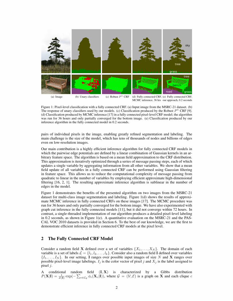
(a) Image (b) Unary classifiers (c) Robust Pn CRF (d) Fully connected CRF,MCMC inference, 36 hrs

sky

tree

grass

bench

tree

road grass

(e) Fully connected CRF,our approach, 0.2 seconds

Figure 1: Pixel-level classification with a fully connected CRF. (a) Input image from the MSRC-21 dataset. (b)The response of unary classifiers used by our models. (c) Classification produced by the Robust Pn CRF [9].(d) Classification produced by MCMC inference [17] in a fully connected pixel-level CRF model; the algorithmwas run for 36 hours and only partially converged for the bottom image. (e) Classification produced by ourinference algorithm in the fully connected model in 0.2 seconds.

pairs of individual pixels in the image, enabling greatly refined segmentation and labeling. Themain challenge is the size of the model, which has tens of thousands of nodes and billions of edgeseven on low-resolution images.

Our main contribution is a highly efficient inference algorithm for fully connected CRF models inwhich the pairwise edge potentials are defined by a linear combination of Gaussian kernels in an ar-bitrary feature space. The algorithm is based on a mean field approximation to the CRF distribution.This approximation is iteratively optimized through a series of message passing steps, each of whichupdates a single variable by aggregating information from all other variables. We show that a meanfield update of all variables in a fully connected CRF can be performed using Gaussian filteringin feature space. This allows us to reduce the computational complexity of message passing fromquadratic to linear in the number of variables by employing efficient approximate high-dimensionalfiltering [16, 2, 1]. The resulting approximate inference algorithm is sublinear in the number ofedges in the model.

Figure 1 demonstrates the benefits of the presented algorithm on two images from the MSRC-21dataset for multi-class image segmentation and labeling. Figure 1(d) shows the results of approxi-mate MCMC inference in fully connected CRFs on these images [17]. The MCMC procedure wasrun for 36 hours and only partially converged for the bottom image. We have also experimented withgraph cut inference in the fully connected models [11], but it did not converge within 72 hours. Incontrast, a single-threaded implementation of our algorithm produces a detailed pixel-level labelingin 0.2 seconds, as shown in Figure 1(e). A quantitative evaluation on the MSRC-21 and the PAS-CAL VOC 2010 datasets is provided in Section 6. To the best of our knowledge, we are the first todemonstrate efficient inference in fully connected CRF models at the pixel level.

2 The Fully Connected CRF Model

Consider a random field X defined over a set of variables {X1, . . . , XN}. The domain of eachvariable is a set of labels L = {l1, l2, . . . , lk}. Consider also a random field I defined over variables{I1, . . . , IN}. In our setting, I ranges over possible input images of size N and X ranges overpossible pixel-level image labelings. Ij is the color vector of pixel j and Xj is the label assigned topixel j.

A conditional random field (I,X) is characterized by a Gibbs distributionP (X|I) = 1

Z(I) exp(−∑c∈CG φc(Xc|I)), where G = (V, E) is a graph on X and each clique c

2

in a set of cliques CG in G induces a potential φc [15]. The Gibbs energy of a labeling x ∈ LNis E(x|I) =

∑c∈CG φc(xc|I). The maximum a posteriori (MAP) labeling of the random field is

x∗ = arg maxx∈LN P (x|I). For notational convenience we will omit the conditioning in the rest ofthe paper and use ψc(xc) to denote φc(xc|I).

In the fully connected pairwise CRF model, G is the complete graph on X and CG is the set of allunary and pairwise cliques. The corresponding Gibbs energy is

E(x) =∑i

ψu(xi) +∑i<j

ψp(xi, xj), (1)

where i and j range from 1 to N . The unary potential ψu(xi) is computed independently for eachpixel by a classifier that produces a distribution over the label assignment xi given image features.The unary potential used in our implementation incorporates shape, texture, location, and colordescriptors and is described in Section 5. Since the output of the unary classifier for each pixelis produced independently from the outputs of the classifiers for other pixels, the MAP labelingproduced by the unary classifiers alone is generally noisy and inconsistent, as shown in Figure 1(b).

The pairwise potentials in our model have the form

ψp(xi, xj) = µ(xi, xj)∑Km=1 w

(m)k(m)(fi, fj)︸ ︷︷ ︸k(fi,fj)

, (2)

where each k(m) is a Gaussian kernel k(m)(fi, fj) = exp(− 12 (fi − fj)

TΛ(m)(fi − fj)), the vectors fiand fj are feature vectors for pixels i and j in an arbitrary feature space, w(m) are linear combinationweights, and µ is a label compatibility function. Each kernel k(m) is characterized by a symmetric,positive-definite precision matrix Λ(m), which defines its shape.

For multi-class image segmentation and labeling we use contrast-sensitive two-kernel potentials,defined in terms of the color vectors Ii and Ij and positions pi and pj :

k(fi, fj) = w(1) exp

(−|pi − pj |

2

2θ2α

− |Ii − Ij |2

2θ2β

)︸ ︷︷ ︸

appearance kernel

+w(2) exp

(−|pi − pj |

2

2θ2γ

)︸ ︷︷ ︸

smoothness kernel

. (3)

The appearance kernel is inspired by the observation that nearby pixels with similar color are likelyto be in the same class. The degrees of nearness and similarity are controlled by parameters θα andθβ . The smoothness kernel removes small isolated regions [19]. The parameters are learned fromdata, as described in Section 4.

A simple label compatibility function µ is given by the Potts model, µ(xi, xj) = [xi 6= xj ]. Itintroduces a penalty for nearby similar pixels that are assigned different labels. While this simplemodel works well in practice, it is insensitive to compatibility between labels. For example, itpenalizes a pair of nearby pixels labeled “sky” and “bird” to the same extent as pixels labeled “sky”and “cat”. We can instead learn a general symmetric compatibility function µ(xi, xj) that takesinteractions between labels into account, as described in Section 4.

3 Efficient Inference in Fully Connected CRFs

Our algorithm is based on a mean field approximation to the CRF distribution. This approxima-tion yields an iterative message passing algorithm for approximate inference. Our key observationis that message passing in the presented model can be performed using Gaussian filtering in fea-ture space. This enables us to utilize highly efficient approximations for high-dimensional filtering,which reduce the complexity of message passing from quadratic to linear, resulting in an approxi-mate inference algorithm for fully connected CRFs that is linear in the number of variables N andsublinear in the number of edges in the model.

3.1 Mean Field Approximation

Instead of computing the exact distribution P (X), the mean field approximation computes a dis-tribution Q(X) that minimizes the KL-divergence D(Q‖P ) among all distributions Q that can beexpressed as a product of independent marginals, Q(X) =

∏iQi(Xi) [10].

3

Minimizing the KL-divergence, while constraining Q(X) and Qi(Xi) to be valid distributions,yields the following iterative update equation:

Qi(xi = l) =1

Ziexp

−ψu(xi)−∑l′∈L

µ(l, l′)

K∑m=1

w(m)∑j 6=i

k(m)(fi, fj)Qj(l′)

. (4)

A detailed derivation of Equation 4 is given in the supplementary material. This update equationleads to the following inference algorithm:

Algorithm 1 Mean field in fully connected CRFs

Initialize Q . Qi(xi)← 1Zi

exp{−φu(xi)}while not converged do . See Section 6 for convergence analysis

Q(m)i (l)←

∑j 6=i k

(m)(fi, fj)Qj(l) for all m . Message passing from all Xj to all Xi

Qi(xi)←∑l∈L µ

(m)(xi, l)∑m w

(m)Q(m)i (l) . Compatibility transform

Qi(xi)← exp{−ψu(xi)− Qi(xi)} . Local updatenormalize Qi(xi)

end while

Each iteration of Algorithm 1 performs a message passing step, a compatibility transform, and alocal update. Both the compatibility transform and the local update run in linear time and are highlyefficient. The computational bottleneck is message passing. For each variable, this step requiresevaluating a sum over all other variables. A naive implementation thus has quadratic complexity inthe number of variables N . Next, we show how approximate high-dimensional filtering can be usedto reduce the computational cost of message passing to linear.

3.2 Efficient Message Passing Using High-Dimensional Filtering

From a signal processing standpoint, the message passing step can be expressed as a convolutionwith a Gaussian kernel GΛ(m) in feature space:

Q(m)i (l) =

∑j∈V k

(m)(fi, fj)Qj(l)−Qi(l)︸ ︷︷ ︸message passing

= [GΛ(m) ⊗Q(l)] (fi)︸ ︷︷ ︸Q

(m)i (l)

−Qi(l). (5)

We subtract Qi(l) from the convolved function Q(m)

i (l) because the convolution sums over all vari-ables, while message passing does not sum over Qi.

This convolution performs a low-pass filter, essentially band-limiting Q(m)

i (l). By the samplingtheorem, this function can be reconstructed from a set of samples whose spacing is proportionalto the standard deviation of the filter [20]. We can thus perform the convolution by downsamplingQ(l), convolving the samples with GΛ(m) , and upsampling the result at the feature points [16].

Algorithm 2 Efficient message passing: Q(m)

i (l) =∑j∈V k

(m)(fi, fj)Qj(l)

Q↓(l)← downsample(Q(l)) . Downsample∀i∈V↓Q

(m)

↓i (l)←∑j∈V↓ k

(m)(f↓i, f↓j)Q↓j(l) . Convolution on samples f↓

Q(m)

(l)← upsample(Q(m)

↓ (l)) . Upsample

A common approximation to the Gaussian kernel is a truncated Gaussian, where all values beyondtwo standard deviations are set to zero. Since the spacing of the samples is proportional to the stan-dard deviation, the support of the truncated kernel contains only a constant number of sample points.Thus the convolution can be approximately computed at each sample by aggregating values fromonly a constant number of neighboring samples. This implies that approximate message passing canbe performed in O(N) time [16].

High-dimensional filtering algorithms that follow this approach can still have computational com-plexity exponential in d. However, a clever filtering scheme can reduce the complexity of the con-volution operation to O(Nd). We use the permutohedral lattice, a highly efficient convolution data

4

structure that tiles the feature space with simplices arranged along d+1 axes [1]. The permutohedrallattice exploits the separability of unit variance Gaussian kernels. Thus we need to apply a whiteningtransform f = U f to the feature space in order to use it. The whitening transformation is found us-ing the Cholesky decomposition of Λ(m) into UUT. In the transformed space, the high-dimensionalconvolution can be separated into a sequence of one-dimensional convolutions along the axes of thelattice. The resulting approximate message passing procedure is highly efficient even with a fullysequential implementation that does not make use of parallelism or the streaming capabilities ofgraphics hardware, which can provide further acceleration if desired.

4 Learning

We learn the parameters of the model by piecewise training. First, the boosted unary classifiers aretrained using the JointBoost algorithm [21], using the features described in Section 5. Next we learnthe appearance kernel parameters w(1), θα, and θβ for the Potts model. w(1) can be found efficientlyby a combination of expectation maximization and high-dimensional filtering. Unfortunately, thekernel widths θα and θβ cannot be computed effectively with this approach, since their gradientinvolves a sum of non-Gaussian kernels, which are not amenable to the same acceleration techniques.We found it to be more efficient to use grid search on a holdout validation set for all three kernelparameters w(1), θα and θβ .

The smoothness kernel parameters w(2) and θγ do not significantly affect classification accuracy,but yield a small visual improvement. We found w(2) = θγ = 1 to work well in practice.

The compatibility parameters µ(a, b) = µ(b, a) are learned using L-BFGS to maximize the log-likelihood `(µ : I, T ) of the model for a validation set of images I with corresponding groundtruth labelings T . L-BFGS requires the computation of the gradient of `, which is intractable toestimate exactly, since it requires computing the gradient of the partition function Z. Instead, weuse the mean field approximation described in Section 3 to estimate the gradient of Z. This leads toa simple approximation of the gradient for each training image:

∂

∂µ(a, b)`(µ : I(n), T (n)) ≈ −

∑i

T (n)i (a)

∑j 6=i

k(fi, fj)T (n)j (b) +

∑i

Qi(a)∑j 6=i

k(fi, fj)Qi(b),

(6)

where (I(n), T (n)) is a single training image with its ground truth labeling and T (n)(a) is a binaryimage in which the ith pixel T (n)

i (a) has value 1 if the ground truth label at the ith pixel of T (n) isa and 0 otherwise. A detailed derivation of Equation 6 is given in the supplementary material.

The sums∑j 6=i k(fi, fj)Tj(b) and

∑j 6=i k(fi, fj)Qi(b) are both computationally expensive to eval-

uate directly. As in Section 3.2, we use high-dimensional filtering to compute both sums efficiently.The runtime of the final learning algorithm is linear in the number of variables N .

5 Implementation

The unary potentials used in our implementation are derived from TextonBoost [19, 13]. We usethe 17-dimensional filter bank suggested by Shotton et al. [19], and follow Ladicky et al. [13] byadding color, histogram of oriented gradients (HOG), and pixel location features. Our evaluationon the MSRC-21 dataset uses this extended version of TextonBoost for the unary potentials. Forthe VOC 2010 dataset we include the response of bounding box object detectors [4] for each objectclass as 20 additional features. This increases the performance of the unary classifiers on the VOC2010 from 13% to 22%. We gain an additional 5% by training a logistic regression classifier on theresponses of the boosted classifier.

For efficient high-dimensional filtering, we use a publicly available implementation of the permuto-hedral lattice [1]. We found a downsampling rate of one standard deviation to work best for all ourexperiments. Sampling-based filtering algorithms underestimate the edge strength k(fi, fj) for verysimilar feature points. Proper normalization can cancel out most of this error. The permutohedrallattice allows for two types of normalizations. A global normalization by the average kernel strength

5

k = 1N

∑i,j k(fi, fj) can correct for constant error. A pixelwise normalization by ki =

∑j k(fi, fj)

handles regional errors as well, but violates the CRF symmetry assumption ψp(xi, xj) = ψp(xj , xi).We found the pixelwise normalization to work better in practice.

6 Evaluation

We evaluate the presented algorithm on two standard benchmarks for multi-class image segmen-tation and labeling. The first is the MSRC-21 dataset, which consists of 591 color images of size320 × 213 with corresponding ground truth labelings of 21 object classes [19]. The second is thePASCAL VOC 2010 dataset, which contains 1928 color images of size approximately 500 × 400,with a total of 20 object classes and one background class [3]. The presented approach was evalu-ated alongside the adjacency (grid) CRF of Shotton et al. [19] and the Robust Pn CRF of Kohli etal. [9], using publicly available reference implementations. To ensure a fair comparison, all modelsused the unary potentials described in Section 5. All experiments were conducted on an Intel i7-930processor clocked at 2.80GHz. Eight CPU cores were used for training; all other experiments wereperformed on a single core. The inference algorithm was implemented in a single CPU thread.

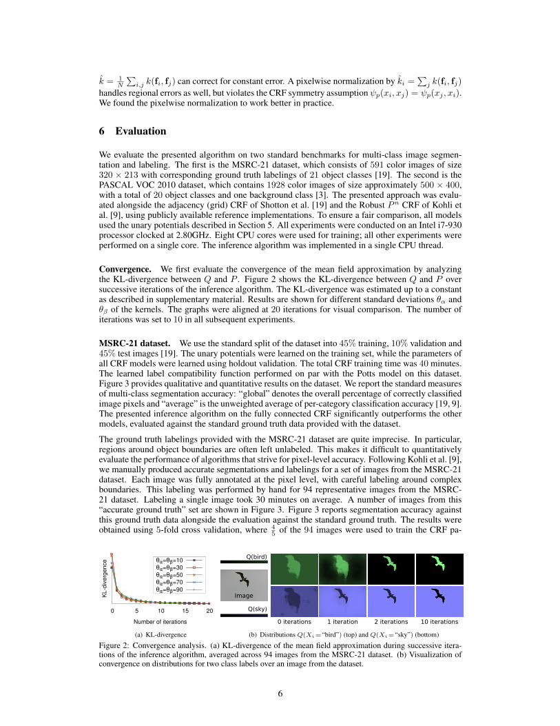
Convergence. We first evaluate the convergence of the mean field approximation by analyzingthe KL-divergence between Q and P . Figure 2 shows the KL-divergence between Q and P oversuccessive iterations of the inference algorithm. The KL-divergence was estimated up to a constantas described in supplementary material. Results are shown for different standard deviations θα andθβ of the kernels. The graphs were aligned at 20 iterations for visual comparison. The number ofiterations was set to 10 in all subsequent experiments.

MSRC-21 dataset. We use the standard split of the dataset into 45% training, 10% validation and45% test images [19]. The unary potentials were learned on the training set, while the parameters ofall CRF models were learned using holdout validation. The total CRF training time was 40 minutes.The learned label compatibility function performed on par with the Potts model on this dataset.Figure 3 provides qualitative and quantitative results on the dataset. We report the standard measuresof multi-class segmentation accuracy: “global” denotes the overall percentage of correctly classifiedimage pixels and “average” is the unweighted average of per-category classification accuracy [19, 9].The presented inference algorithm on the fully connected CRF significantly outperforms the othermodels, evaluated against the standard ground truth data provided with the dataset.

The ground truth labelings provided with the MSRC-21 dataset are quite imprecise. In particular,regions around object boundaries are often left unlabeled. This makes it difficult to quantitativelyevaluate the performance of algorithms that strive for pixel-level accuracy. Following Kohli et al. [9],we manually produced accurate segmentations and labelings for a set of images from the MSRC-21dataset. Each image was fully annotated at the pixel level, with careful labeling around complexboundaries. This labeling was performed by hand for 94 representative images from the MSRC-21 dataset. Labeling a single image took 30 minutes on average. A number of images from this“accurate ground truth” set are shown in Figure 3. Figure 3 reports segmentation accuracy againstthis ground truth data alongside the evaluation against the standard ground truth. The results wereobtained using 5-fold cross validation, where 4

5 of the 94 images were used to train the CRF pa-

0 5 10 15 20

KL-

dive

rgen

ce

Number of iterations

θα=θβ=10 θα=θβ=30 θα=θβ=50 θα=θβ=70 θα=θβ=90

(a) KL-divergence

Image

Q(sky)

Q(bird)

0 iterations 1 iteration 2 iterations 10 iterations

(b) Distributions Q(Xi =“bird”) (top) and Q(Xi =“sky”) (bottom)

Figure 2: Convergence analysis. (a) KL-divergence of the mean field approximation during successive itera-tions of the inference algorithm, averaged across 94 images from the MSRC-21 dataset. (b) Visualization ofconvergence on distributions for two class labels over an image from the dataset.

6

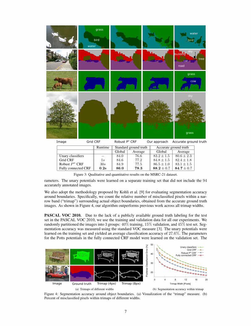
Image Grid CRF Robust Pn CRF Our approach Accurate ground truth

bird

water

road

car

sky

tree

building

grass

cow

sky

tree

grass

grass

water

bird

Runtime Standard ground truth Accurate ground truthGlobal Average Global Average

Unary classifiers − 84.0 76.6 83.2± 1.5 80.6± 2.3Grid CRF 1s 84.6 77.2 84.8± 1.5 82.4± 1.8Robust Pn CRF 30s 84.9 77.5 86.5± 1.0 83.1± 1.5Fully connected CRF 0.2s 86.0 78.3 88.2± 0.7 84.7± 0.7

Figure 3: Qualitative and quantitative results on the MSRC-21 dataset.

rameters. The unary potentials were learned on a separate training set that did not include the 94accurately annotated images.

We also adopt the methodology proposed by Kohli et al. [9] for evaluating segmentation accuracyaround boundaries. Specifically, we count the relative number of misclassified pixels within a nar-row band (“trimap”) surrounding actual object boundaries, obtained from the accurate ground truthimages. As shown in Figure 4, our algorithm outperforms previous work across all trimap widths.

PASCAL VOC 2010. Due to the lack of a publicly available ground truth labeling for the testset in the PASCAL VOC 2010, we use the training and validation data for all our experiments. Werandomly partitioned the images into 3 groups: 40% training, 15% validation, and 45% test set. Seg-mentation accuracy was measured using the standard VOC measure [3]. The unary potentials werelearned on the training set and yielded an average classification accuracy of 27.6%. The parametersfor the Potts potentials in the fully connected CRF model were learned on the validation set. The

Image Ground truth Trimap (4px) Trimap (8px)

(a) Trimaps of different widths

20

30

40

50

0 4 8 12 16 20

Pix

elw

ise

Cla

ssifi

actio

n E

rror

[%]

Trimap Width [Pixels]

Unary classifiersGrid CRF

Robust Pn CRFFully connected CRF

(b) Segmentation accuracy within trimap

Figure 4: Segmentation accuracy around object boundaries. (a) Visualization of the “trimap” measure. (b)Percent of misclassified pixels within trimaps of different widths.

7

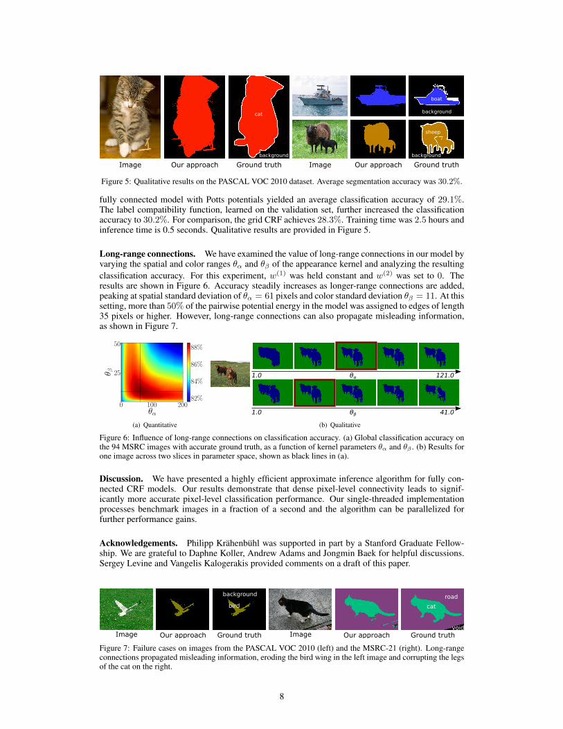
Image Ground truth

cat

background

Our approach Ground truth

boat

background

sheep

background

Our approachImage

Figure 5: Qualitative results on the PASCAL VOC 2010 dataset. Average segmentation accuracy was 30.2%.

fully connected model with Potts potentials yielded an average classification accuracy of 29.1%.The label compatibility function, learned on the validation set, further increased the classificationaccuracy to 30.2%. For comparison, the grid CRF achieves 28.3%. Training time was 2.5 hours andinference time is 0.5 seconds. Qualitative results are provided in Figure 5.

Long-range connections. We have examined the value of long-range connections in our model byvarying the spatial and color ranges θα and θβ of the appearance kernel and analyzing the resultingclassification accuracy. For this experiment, w(1) was held constant and w(2) was set to 0. Theresults are shown in Figure 6. Accuracy steadily increases as longer-range connections are added,peaking at spatial standard deviation of θα = 61 pixels and color standard deviation θβ = 11. At thissetting, more than 50% of the pairwise potential energy in the model was assigned to edges of length35 pixels or higher. However, long-range connections can also propagate misleading information,as shown in Figure 7.

0 100 200θα

25

50

θ β

82%

84%

86%

88%

(a) Quantitative

θα1.0 121.0

θβ1.0 41.0

(b) Qualitative

Figure 6: Influence of long-range connections on classification accuracy. (a) Global classification accuracy onthe 94 MSRC images with accurate ground truth, as a function of kernel parameters θα and θβ . (b) Results forone image across two slices in parameter space, shown as black lines in (a).

Discussion. We have presented a highly efficient approximate inference algorithm for fully con-nected CRF models. Our results demonstrate that dense pixel-level connectivity leads to signif-icantly more accurate pixel-level classification performance. Our single-threaded implementationprocesses benchmark images in a fraction of a second and the algorithm can be parallelized forfurther performance gains.

Acknowledgements. Philipp Krahenbuhl was supported in part by a Stanford Graduate Fellow-ship. We are grateful to Daphne Koller, Andrew Adams and Jongmin Baek for helpful discussions.Sergey Levine and Vangelis Kalogerakis provided comments on a draft of this paper.

Image Our approach Ground truth Image Our approach Ground truth

bird

background

void

road

cat

Figure 7: Failure cases on images from the PASCAL VOC 2010 (left) and the MSRC-21 (right). Long-rangeconnections propagated misleading information, eroding the bird wing in the left image and corrupting the legsof the cat on the right.

8

References[1] A. Adams, J. Baek, and M. A. Davis. Fast high-dimensional filtering using the permutohedral lattice.

Computer Graphics Forum, 29(2), 2010. 2, 5

[2] A. Adams, N. Gelfand, J. Dolson, and M. Levoy. Gaussian kd-trees for fast high-dimensional filtering.ACM Transactions on Graphics, 28(3), 2009. 2

[3] M. Everingham, L. Van Gool, C. K. I. Williams, J. Winn, and A. Zisserman. The PASCAL Visual ObjectClasses (VOC) challenge. IJCV, 88(2), 2010. 6, 7

[4] P. F. Felzenszwalb, R. B. Girshick, and D. A. McAllester. Cascade object detection with deformable partmodels. In Proc. CVPR, 2010. 5

[5] B. Fulkerson, A. Vedaldi, and S. Soatto. Class segmentation and object localization with superpixelneighborhoods. In Proc. ICCV, 2009. 1

[6] C. Galleguillos, A. Rabinovich, and S. Belongie. Object categorization using co-occurrence, location andappearance. In Proc. CVPR, 2008. 1

[7] S. Gould, J. Rodgers, D. Cohen, G. Elidan, and D. Koller. Multi-class segmentation with relative locationprior. IJCV, 80(3), 2008. 1

[8] X. He, R. S. Zemel, and M. A. Carreira-Perpinan. Multiscale conditional random fields for image labeling.In Proc. CVPR, 2004. 1

[9] P. Kohli, L. Ladicky, and P. H. S. Torr. Robust higher order potentials for enforcing label consistency.IJCV, 82(3), 2009. 1, 2, 6, 7

[10] D. Koller and N. Friedman. Probabilistic Graphical Models: Principles and Techniques. MIT Press,2009. 3

[11] V. Kolmogorov and R. Zabih. What energy functions can be minimized via graph cuts? PAMI, 26(2),2004. 2

[12] S. Kumar and M. Hebert. A hierarchical field framework for unified context-based classification. In Proc.ICCV, 2005. 1

[13] L. Ladicky, C. Russell, P. Kohli, and P. H. S. Torr. Associative hierarchical crfs for object class imagesegmentation. In Proc. ICCV, 2009. 1, 5

[14] L. Ladicky, C. Russell, P. Kohli, and P. H. S. Torr. Graph cut based inference with co-occurrence statistics.In Proc. ECCV, 2010. 1

[15] J. D. Lafferty, A. McCallum, and F. C. N. Pereira. Conditional random fields: Probabilistic models forsegmenting and labeling sequence data. In Proc. ICML, 2001. 3

[16] S. Paris and F. Durand. A fast approximation of the bilateral filter using a signal processing approach.IJCV, 81(1), 2009. 2, 4

[17] N. Payet and S. Todorovic. (RF)2 – random forest random field. In Proc. NIPS. 2010. 1, 2

[18] A. Rabinovich, A. Vedaldi, C. Galleguillos, E. Wiewiora, and S. Belongie. Objects in context. In Proc.ICCV, 2007. 1

[19] J. Shotton, J. M. Winn, C. Rother, and A. Criminisi. Textonboost for image understanding: Multi-classobject recognition and segmentation by jointly modeling texture, layout, and context. IJCV, 81(1), 2009.1, 3, 5, 6

[20] S. W. Smith. The scientist and engineer’s guide to digital signal processing. California Technical Pub-lishing, 1997. 4

[21] A. Torralba, K. P. Murphy, and W. T. Freeman. Sharing visual features for multiclass and multiview objectdetection. PAMI, 29(5), 2007. 5

[22] T. Toyoda and O. Hasegawa. Random field model for integration of local information and global infor-mation. PAMI, 30, 2008. 1

[23] J. J. Verbeek and B. Triggs. Scene segmentation with crfs learned from partially labeled images. In Proc.NIPS, 2007. 1

9