IT 11 069

Examensarbete 30 hpSeptember 2011

Efficient Implementation of Polyline Simplification for Large Datasets and Usability Evaluation

Institutionen för informationsteknologiDepartment of Information Technology

Şadan Ekdemir

Teknisk- naturvetenskaplig fakultet UTH-enheten

Besöksadress: Ångströmlaboratoriet Lägerhyddsvägen 1 Hus 4, Plan 0

Postadress: Box 536 751 21 Uppsala

Telefon:018 – 471 30 03

Telefax: 018 – 471 30 00

Hemsida:http://www.teknat.uu.se/student

Abstract

Efficient Implementation of Polyline Simplification forLarge Datasets and Usability Evaluation

An in-depth analysis and survey of polyline simplification routines is performed withinthe project. The research is conducted using different simplification routines andperforming evaluative tests on the outputs of each simplification routine. The projectlies in between two major fields, namely Computer Graphics and Cartography,combining the needs of both sides and uses the algorithms that are developed foreach field. After the implementation of the algorithms, a scientific survey is performedby comparing them according to the evaluation benchmarks, which are performance,reduction rate and visual similarity. Apart from the existing routines, one newsimplification routine, triangular routine is developed and recursive Douglas-Peuckerroutine is converted into non-recursive. As a preprocessing part, Gaussian smoothingkernel is used to reduce noise and complexity of the polyline, and betterperformances are achieved. The end of research shows that there is no best modelinstead there are advantages and disadvantages of each simplification routine,depending on the prior need. It is also shown that usage of Gaussian smoothing as afiltering process improves the performance of each simplification routine.

Tryckt av: Reprocentralen ITCIT 11 069Examinator: Anders JanssonÄmnesgranskare: Stefan SeipelHandledare: Jörn Letnes

Şadan Ekdemir

To all, whom I met in my life that taught me how to live, how to think,how to feel and how to comprehend the world.

And to my grandfather, who has unfortunately passed away this summer.

Not of a greater debt that I have to my dear parents,to my sister, Sibel for her invaluable support, for

holding my hand within each step I have taken in life,to my friends, and Susanne for giving me peace, I owe.

Acknowledgments

First and foremost, I would like to thank to my parents and my sister for all their invaluablesupport on my survey of finding what I actually want to do in my life, and that I could havebrought myself so far.

I owe a big thank to my dear teacher, Maya Neytcheva for giving me self confidence in theproject work I did with her, and introducing me an amazing option for my thesis project andproviding contact people from the Schlumberger Company. Special thanks to Jørn Letnes, whohas been the supervisor of my thesis project and his inputs on my project progress. Also toStefan Seipel, my reviewer, who has been overseeing my thesis project project and providinghis own ideas.

Apart from all, I would like to thank Cris Luego, who has been great of help to with all hisvoluntarily and invaluable support and interest on my thesis project, generating new ideas andassisting me with my never ending questions. Lastly, very special thanks to Elmar de Koningfor his inspirational work on polyline simplification and his personal support on my project.

Computer Graphics has been my favorite field, and I am deeply thankful to everyone whomade this project possible.

Contents

1 Background 1

2 Objectives 2

3 Related Work 3

4 Theory and Applications 44.1 Line simplification algorithms . . . . . . . . . . . . . . . . . . . . . . . . . . . . . 54.2 Independent point routines . . . . . . . . . . . . . . . . . . . . . . . . . . . . . . 5

4.2.1 Nth point routine . . . . . . . . . . . . . . . . . . . . . . . . . . . . . . . . 64.3 Local Processing Routines . . . . . . . . . . . . . . . . . . . . . . . . . . . . . . . 6

4.3.1 Reumann-Witkam Routine . . . . . . . . . . . . . . . . . . . . . . . . . . 74.3.2 Triangular Routine . . . . . . . . . . . . . . . . . . . . . . . . . . . . . . . 84.3.3 Lang Routine . . . . . . . . . . . . . . . . . . . . . . . . . . . . . . . . . . 10

4.4 Global Routines . . . . . . . . . . . . . . . . . . . . . . . . . . . . . . . . . . . . . 114.4.1 Douglas-Peucker Routine . . . . . . . . . . . . . . . . . . . . . . . . . . . 11

4.5 Line smoothing . . . . . . . . . . . . . . . . . . . . . . . . . . . . . . . . . . . . . 114.6 Measurement & Error Analysis for Line Simplification . . . . . . . . . . . . . . . 15

5 Methods 195.1 Modified Algorithms . . . . . . . . . . . . . . . . . . . . . . . . . . . . . . . . . . 19

5.1.1 Converting recursive Douglas-Peucker algorithm into non-recursive . . . . 195.1.2 Employing Gaussian filtering as part of simplification . . . . . . . . . . . 20

5.2 Implementations . . . . . . . . . . . . . . . . . . . . . . . . . . . . . . . . . . . . 215.3 Algorithms . . . . . . . . . . . . . . . . . . . . . . . . . . . . . . . . . . . . . . . 225.4 Determination of tolerance value and handling random datasets . . . . . . . . . . 265.5 Evaluation methods . . . . . . . . . . . . . . . . . . . . . . . . . . . . . . . . . . 27

6 Results 286.1 Work Bench . . . . . . . . . . . . . . . . . . . . . . . . . . . . . . . . . . . . . . . 286.2 Evaluation of the line simplification algorithms . . . . . . . . . . . . . . . . . . . 29

6.2.1 Performance Analysis . . . . . . . . . . . . . . . . . . . . . . . . . . . . . 296.2.2 Reduction rate comparison . . . . . . . . . . . . . . . . . . . . . . . . . . 326.2.3 Dissimilarity measure comparison . . . . . . . . . . . . . . . . . . . . . . . 326.2.4 Lang routine parameterization . . . . . . . . . . . . . . . . . . . . . . . . 35

6.3 Gaussian smoothing . . . . . . . . . . . . . . . . . . . . . . . . . . . . . . . . . . 35

7 Discussion & Conclusions 42

8 Future Work 45

9 Appendix 46

1 Background

In computer graphics, polygonal models currently dominate a huge portion in interactivity.This is mainly because of their mathematical simplicity; polygonal models lend themselves tosimple, regular rendering algorithms that is embedded well in hardware, which has a significantrendering acceleration in turn. However, the complexity of these models seem to grow fasterthan the ability of our graphics hardware to render them interactively. In other words, thenumber of polygons we want always has the tendency to exceed the number of polygons we canafford.

As a solution to that problem, various polygonal simplification techniques are used forgrappling with complex polygonal models. The main function of these methods is to simplifythe polygonal geometry of small, distant, or unimportant portions, looking for available partsto reduce the rendering cost without a significant loss in the visual content of what is seen onthe scene [?]. Indeed, this is a both current and a very old idea in computer graphics, thanks tothe research of James Clark, Communications of the ACM, in 1976 [?], which is called levels-of-details. At that time, computers were monolithic and rare, and work on graphics was mainlydriven by researchers. The hardware itself was completely different, both architecturally andperformance-wise. Therefore the simplification was a crucial factor in terms of performance.The following figure depicts one example of level-of-detail on 3-dimensional modeling 1.

Figure 1: Representation of LOD in action on computer generated version of Mozart’s statue

The original algorithm was presented as a generic approach which would be convenient forall kinds of polygonal operations with the following concern: ’Increased complexity of a scene,or increased information in the database, has less value as the resolution limits of the displayare approached. It makes no sense to use 500 polygons describing an object if it only covers20 raster units of the display.’ Then comes the actual question: How can we select only theportion of the database that has meaning in the context of the resolution of the viewing device?To put in other way, we would like to present the minimal information needed to convey themeaning of what is being viewed. As an example, if we are to view a human body from a suffi-ciently large distance, we might only need to present the ’specks’ for the eyes, and perhaps justa block for the head, instead of presenting the entire details and features of the body and face. [2]

With no doubt, there are various need for the simplification of polygonal objects, to eliminatethe redundant geometry in volumetric surfaces, or reducing model size for a comprehensive and

1Image is generated by using OpenSG 2 Vision (http://www.opensg.org/)

1

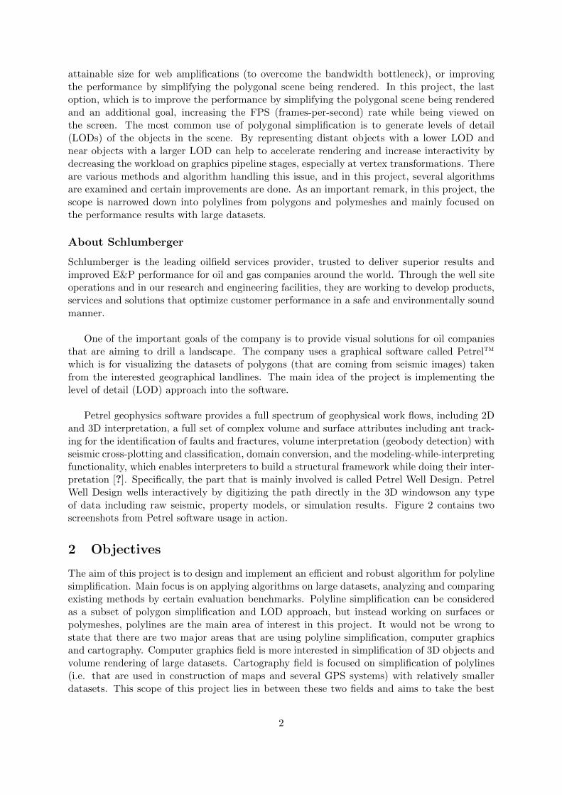
attainable size for web amplifications (to overcome the bandwidth bottleneck), or improvingthe performance by simplifying the polygonal scene being rendered. In this project, the lastoption, which is to improve the performance by simplifying the polygonal scene being renderedand an additional goal, increasing the FPS (frames-per-second) rate while being viewed onthe screen. The most common use of polygonal simplification is to generate levels of detail(LODs) of the objects in the scene. By representing distant objects with a lower LOD andnear objects with a larger LOD can help to accelerate rendering and increase interactivity bydecreasing the workload on graphics pipeline stages, especially at vertex transformations. Thereare various methods and algorithm handling this issue, and in this project, several algorithmsare examined and certain improvements are done. As an important remark, in this project, thescope is narrowed down into polylines from polygons and polymeshes and mainly focused onthe performance results with large datasets.

About Schlumberger

Schlumberger is the leading oilfield services provider, trusted to deliver superior results andimproved E&P performance for oil and gas companies around the world. Through the well siteoperations and in our research and engineering facilities, they are working to develop products,services and solutions that optimize customer performance in a safe and environmentally soundmanner.

One of the important goals of the company is to provide visual solutions for oil companiesthat are aiming to drill a landscape. The company uses a graphical software called Petreltm

which is for visualizing the datasets of polygons (that are coming from seismic images) takenfrom the interested geographical landlines. The main idea of the project is implementing thelevel of detail (LOD) approach into the software.

Petrel geophysics software provides a full spectrum of geophysical work flows, including 2Dand 3D interpretation, a full set of complex volume and surface attributes including ant track-ing for the identification of faults and fractures, volume interpretation (geobody detection) withseismic cross-plotting and classification, domain conversion, and the modeling-while-interpretingfunctionality, which enables interpreters to build a structural framework while doing their inter-pretation [?]. Specifically, the part that is mainly involved is called Petrel Well Design. PetrelWell Design wells interactively by digitizing the path directly in the 3D windowson any typeof data including raw seismic, property models, or simulation results. Figure 2 contains twoscreenshots from Petrel software usage in action.

2 Objectives

The aim of this project is to design and implement an efficient and robust algorithm for polylinesimplification. Main focus is on applying algorithms on large datasets, analyzing and comparingexisting methods by certain evaluation benchmarks. Polyline simplification can be consideredas a subset of polygon simplification and LOD approach, but instead working on surfaces orpolymeshes, polylines are the main area of interest in this project. It would not be wrong tostate that there are two major areas that are using polyline simplification, computer graphicsand cartography. Computer graphics field is more interested in simplification of 3D objects andvolume rendering of large datasets. Cartography field is focused on simplification of polylines(i.e. that are used in construction of maps and several GPS systems) with relatively smallerdatasets. This scope of this project lies in between these two fields and aims to take the best

2

Figure 2: Screenshots of Petrel

sides of these two fields in order to get an efficient implementation of simplification. The meth-ods developed for polyline simplifications are used in both fields and in this report, some ofthose methods are discussed and several improvements are performed.

3 Related Work

As it is stated, polyline (or polygon) simplification approach is both used in Computer Graphicsfield (LOD) and also in Cartography field. Before going deep into the project, the reader mightwonder the usage areas of the simplification approach in both fields. The major need for LODapproach in graphics field has risen when virtual reality applications exceed the capacity ofmodern graphical hardware. These scenes have complex structures and their display requiresa huge number of polygons, even when only a little portion of the scene that is visible for thegiven frame. In 1976, it is suggested to use simpler versions of the geometry for objects that

3

had lesser visual importance, such as those would be far away from the viewer, and this simpli-fication approach is called Levels of Details (LODs)[?].

There are many aspects of LODs, one of which is to filter the geometry to produce amodel with fewer polygons. The aim of the polygonal simplification is to remove primitivesfrom an original mesh in order to produce simpler models which retain the important visualcharacteristics of the original object. The idea, in order to maintain a constant frame rate, isto find a good balance between the richness of the models and the time it takes to display them(i.e. rendering time). In terms of describing a way to classify the kinds of hierarchies used tobuild a simplification algorithm, there are three main classes:

• Discrete: Discrete LOD hierarchy encodes a few LODs at very coarse granularity. They aresimple to use, and offer the advanced that each LOD may be converted into an optimizedform of rendering.

• Continuous: This is a very fine-grained discrete LOD hierarchy. It allows more fine-grained selection of the number of primitives to use for representation of the object. Thismethod has many advantages as it can adjust the levels of detail in the run time. Itprovides, better granularity, which leads to have better fidelity and smoother transitionsin different parts of the simplified object.

• View-dependent : This is the most complex form of LOD representation, which allows notonly fine-grained selection of LODs but also permits the detail to be varied across differentportions of the same object, based on viewing parameters. For example, closer portionsof an object can be shown in more detail than farther ones[?].

In Computer Graphics, meshes are the most widely used type of model in LOD applica-tions, whereas in Cartography, polylines and line generalization are used as the type of model.In Computer Graphics, 3-dimensional geometry plays an important role in terms of visual qual-ity, the trade-off between retaining of the details and rendering speed and such, in Cartography,vectorial displacement measure is the key-factor [?]. Moreover, Cartography mainly deals with2-dimensional (or even 1-dimensional) polylines (i.e. landlines in maps and topological rep-resentations), and Computer Graphics deal with meshes and polygonal surfaces. Hence, thealgorithms for LOD varies depending on the usage of the field.

In this project, algorithms for polyline simplification are taken from the ones that are usedin Cartography field, as the main concern is to perform simplification on seismic image repre-sentation, but for the evaluation of the different simplification routines, the criteria which aremainly used by Computer Graphics are used as the software generates a 3-dimensional imageafter the simplification.

4 Theory and Applications

Line simplification is an important function in cartography, for topological representations andalso is widely used in commercial GIS software packages. Most line simplification algorithmsrequire the user to supply a tolerance value, which is used to determine the extent to whichsimplification is to be applied. Apart from that, it is also possible and might be a good optionto determine the optimal tolerance automatically, depending on the variation on the dataset.Simplification algorithms weed from the line redundant or unnecessary coordinate pairs. Themajority of simplification algorithms do not, however, operate by identifying this redundancy,

4

but calculate and retain the prominent features of the polyline. Most simplification routinesselect the critical points based on the topological relationships of points and their neighbors,where the extent of this neighborhood search varies greatly between the algorithms. While suchsimplification routines only retain or eliminate coordinate data, smoothing algorithms displacespoints in attempt to reduce angularity and give the line a more smoother appearance. [?]All line simplification algorithms induce positional errors in the data set, because of the fact thatthey produce a discrepancy between the original line and its simplified version. The amountof this error depends both on the tolerance value and the shape of the line itself. What isusually important from the user perspective, is to maintain a specific level of quality, and notthe tolerance value itself. Furthermore, line simplification involves the selective eliminationof vertices along a line to remove unwanted information. This determining of the removal ofunwanted information is an important process, as it directly effects the visual perceptual qualityof the simplified version[?][?].In order to clarify the need for line simplification and the main considerations for the dataelimination, we can say that there are three major considerations:

• Reduced storage space: this may reduce a dataset, which will result in faster data retrievaland management, and also rendering and putting on the screen

• Faster vector processing: for example, a simplified polygon boundary would enable usto reduce the number of boundary segments to be checked for shading or point to pointinteraction within the polygon

• Reduced rendering time [?]

4.1 Line simplification algorithms

For those and many other reasons which are specified above, there are several line simplifi-cation algorithms and they all have different strengths and weaknesses for specific conditions.Simplification algorithms may be clustered as follows:

• Independent point routines

• Localized processing routines

– Unconstrained extended local processing routines

– Constrained extended local processing routines

• Global routines

4.2 Independent point routines

Independent point algorithms are rather simple in nature and do not take into account the math-ematical relationship of neighboring co-ordinating points. It is basically focused on removing aspecific point which is predefined from the original polyline. An example of this method couldbe the nth point routine.

5

4.2.1 Nth point routine

Nth point routine is a navie O(n) algorithm for polyline simplification. It basically retains onlyfirst, last and each nth point on the origial polyline. As can be imagined, these routines arevery much computationally effective, however, they are not acceptable under the considerationof accuracy, as it doesn’t check any of the curvature information along the polyline[?].

In Figure 3, an illustration of nth point routine can be seen.

Figure 3: Illustration of nth point routine for a 10-point polyline where n=3

The illustration above shows a polyline consisting of 8 vertices: {v1, v2, ... , v8} and thesimplification process by using nth point routine while n = 3. The resulting simplification isincluding vertices: {v1, v4, v7, v8}. The algorithm is extremely fast, but unfortunately it isnot very good at preserving geometric features (i.e. curvature information) of the line. For abetter representation of this unwanted situation, a 100-point polyline with randomized pointsis generated which can be seen on Figure 4. The original line is represented in black and thesimplified version is represented by the red line.

Figure 4: Illustration of nth point routine for a 100-point polyline where n=3

4.3 Local Processing Routines

This category regards a relationship between every two or three consecutive original points.Two examples for this relation can be told as;

• the distance between the two consecutive points

• the perpendicular distance from a line connecting two points to an intermediate point

These distances should not be smaller than their individual tolerance bandwidths (a user de-fined tolerance or angular change). Points within the bandwidth are eliminated, whereas points

6

exceeding the bandwidth are retained. [6] A fundamental routine for this case would be Per-pendicular distance routine, which is illustrated below.

Figure 5: Illustration of perpendicular distance algorithm

Unconstrained Extended Local Processing Routines

This category means that it is an extension to the regular local processing routines, and it doesnot have a constraint; it evaluates relations over sections of the line. One good example for thiscategory is Reumann - Witkam routine.

4.3.1 Reumann-Witkam Routine

The method creates line strip and traverses the original polyline by moving this strip. This striphas the thickness which is the tolerance value (either user defined or calculated) and it is createdby connecting the successive points in the polyline. The first strip is created by connecting thefirst two points of the polyline, and then the strip is shifted over the polyline into the directionof its initial tangent, until the strip hits the line. By following the strip, for each incrementalvertex vi, its perpendicular distance to this line is calculated. A new key index is found at vi-1,when this distance exceeds the specified tolerance value. The vertices vi and vi+1 are thenused to define a new line and line strip. This process is done iteratively, until the last point ofthe polyline is reached[?].

There is one other interesting method under this category, which is a sleeve-fitting polylinesimplification method, proposed by Zhao and Saafeld (1997). The algorithm is similar to theReumann-Witkam routine as it also divides the original line into sections, but not by using linestrips, by using a rectangle (with user defined width). Due to time considerations this methodis not used within the context of the project, therefore will not be explained in detail.

7

Figure 6: Illustration of Reumann-Witkam routine for a 9-point polyline

4.3.2 Triangular Routine

This method is my own invention, idea came to my mind after checking some of the existingalgorithms, especially the one called ’Perpendicular Distance’ routine. Perpendicular distanceroutine is a method that uses a point-to-segment distance tolerance. For each vertex vi, itsperpendicular distance to the segment S(vi-1, vi+1) is computed. All vertices whose distance issmaller than the given tolerance are removed from the original polyline. In action, initially thefirst three vertices of the polyline are processed, and the perpendicular distance of the secondvertex is calculated. After comparing this distance against the tolerance, the second vertex isconsidered to be a part of the simplification. The algorithm continues by moving one vertexup on the polyline and applies the same method for the successive set of three vertices andchecks the perpendicular distances to the line segments. The calculated distance falls below thetolerance and this the intermediate vertex is remoed. The algorithm shifts over the polylineuntil the last point is reached.

What triangular routine does can be described as one step further than the perpendiculardistance routine. After finding the perpendicular distance from the vertix vi to the line segment,the length of the line segment S(vi-1, vi+1) is also computed. So, a triangle T with the vertices

8

T(vi-1, vi, vi+1) is formed with calculated segment and height values. With this information,by applying the geometrical formula to compute the area of triangle, the area is obtained. Ifthe area value of the specific triangle is greater than the tolerance value, the vertex vi is keptand it becomes the new first point for the next triangle. If the condition is not met, vertex viis omitted and the new first point for the next triangle becomes vi+1. This process continuesuntil the last point of the polyline is reached. Figure 7 depicts the triangular routine.

Figure 7: Illustration of triangular routine for a 10-point polyline

The reason why I went for calculating the triangular area is mainly inspired by a mathematicalmeasurement method for line simplification method introduced by McMaster [9]. The arealreplacement between the original and simplified polyline is defined as a criterion of dissimilaritymeasurement for the simplification. Although it works very similar to perpendicular distanceroutine, it differs in the way that it considers both the perpendicular distance between thespecific vertex and the line segment and the length of the line segment as well. This is thoughtto preserve more details in the simplified polygon after the process.

Constrained Extended Local Processing Routines

Constrained extended local processing routines are utilizing the criteria in the unconstrainedextended local processing routines and using additional constraints to define a search regionfor the original line. This search region is used to divide original line into sections and makecalculations. Therefore altering parameters yields different results, which gives more degrees offreedom for the simplification method. An important example for this routine is Lang simplifi-cation algorithm, which was developed by Lang in 1969.

9

4.3.3 Lang Routine

The search region is defined by the user and the perpendicular distance from a segment connect-ing two original points to the original points between them. Each search region is initialized asa region containing a fixed number of consecutive original points. The perpendicular distancesfrom the segment to the intermediate points are calculated and if the calculated distance islarger than the user defined tolerance value, the search region is shrunk by excluding its lastpoint and the distances are calculated again. This process will continue until all the calculatedperpendicular distances from intermediate points are below the user defined tolerance value,or until there are no more intermediate points. Once all the intermediate points are moved, anew search region is defined by stating at last point of the latest (or most recent) search region.This process is repeated and shifted over the original line, until the last point of the polyline isreached[?].

Figure 8: Illustration of lang routine for an 10-point polyline where search region = 5

10

4.4 Global Routines

The methods described above are algorithms which process a line piece by piece, from thebeginning to the end. This category describes a different, more holistic approach to the polylinesimplification. A global routine differs from local routines by considering the line in its entiretywhile processing it. The only existing global simplification algorithm which is commonly usedin both cartography and computer graphics is Douglas Peucker algorithm. This algorithm isnot only a mathematical but also a perceptually superior, as it produces the best results interms of both vector displacement and area displacement.

4.4.1 Douglas-Peucker Routine

Douglas Peucker algorithm is a method that tries to preserve directional trends in a line usinga tolerance factor. This algorithm is also known as the iterative end-point fit algorithm orsplit-and-merge algorithm. In the original paper by Douglas and Peucker, 1973, the authorsdescribe two methods for reducing the number of points required to represent a polyline. Thefirst point on the line is defined as the ’anchor’ and the last point as a ’floater’. These two pointsare connected by a straight line segment and perpendicular distances from this segment to allintervening points are calculated. In the case that none of the perpendicular distances exceed auser specified tolerance (it is a distance value), then the straight line segment is deemed suitableto present the whole line in the simplified form[?].

If the condition is not met, then that specific point with the greatest perpendicular distancefrom the straight line segment is selected as a new floating point. This process is repeated,and a new straight line segment is being defined by the anchor and the new floater. Offsetsfor intervening points are then recalculated as perpendicular to this new segment. This processcontinues; the line is being repeatedly subdivided into subpolylines with selected floating pointsbeing stored in a stack, until the tolerance criteria is met. Once the tolerance criteria is met,the anchor is moved to the most recently selected floater, and the new floating point is selectedfrom the top of the stack of previously selected floaters. This process is repeated successivelyand eventually, the anchor point reaches the last point on the line, and then the simplificationprocess is completed. At the end of this process, points previously assigned as anchors areconnected by a straight line to form a simplified line[?], [?]. Here the important thing to keep inmind is that specifying a low tolerance value results in little line detail being removed whereasspecifying a high tolerance value results in all but the most general features of the line beingremoved. In the Figure 9, Douglas-Peucker routine is illustrated in detail.

At this point, it can be understood that Douglas - Peucker method is a Divide-and-conqueralgorithm, where a polyline is divided into smaller pieces and processed. Such algorithms areknown to be recursive algorithms, as the same task is done for smaller pieces of the originaldataset. Here, the reader should be warned that recursive algorithms are subject to causestack-overflow problems with large datasets, which is the case in my project. Hence, severalmodifications are implemented on the original algorithm to convert it into an iterative, non-recursive algorithm to have a more robust and stable method. Further details can be found inResults section.

4.5 Line smoothing

Smoothing is a process by which data points are averaged with their neighbors in a series, suchas a time series, or image. the biggest usage of smoothing is the image processing, but it isalso used as a filtering method, simply because smoothing has the effect of suppressing high

11

Figure 9: Illustration of Douglas - Peucker routine for an 10-point polyline

frequency signal and enhancing low frequency signal. As Robert B. McMaster has stated in hisarticle in 1992 [?], smoothing algorithms can be used as a part of line simplification algorithms,as they are capable of displacing points in an attempt to reduce angularity and give the linea more flowing appearance. Apart from that, using a smoothing kernel may help to reducethe dataset size as noise can be reduced and less points would be needed to retain the detailsof the original line. Since the dataset type I had in my project is very large and having avery fluctuating character, using smoothing algorithm is thought to be a doable idea for myproject. There are many different methods of smoothing, but in this project, I have used andimplemented smoothing with a Gaussian kernel.Gaussian filter (or kernel) is a windowed filter of linear class, by its nature is weighted mean.Named after famous scientist Carl Gauss because weights in the filter calculated according toGaussian distribution - the function Carl used in his works.The reasons why line smoothing is decided to be used in the project are:

• Reducing the number of data points without losing the curvature information

12

• Reduce the complexity for the usage of global routines (refer to complexity analysis)

Gaussian filter

For 1-Dimensional case, the one-dimensional Gaussian filter has an impulse response given by:

g(x) =

√a

πe−ax

2(1)

and when the standard deviation is added as parameter, we obtain a very general formula:

g(x) =1√2πσ

e−(x−a)2

2σ2 (2)

Here the plot of the equation is depicted below:

Figure 10: Gaussian distribution illustrated

In our 1-dimensional case, we can presume parameter a, which is called distribution meanor statistical expectation, responsible for distribution shifting along x-axis to be zero, i.e. a = 0and then we can obtain the simplified form given below:

g(x) =1√2πσ

e−x2

2σ2 (3)

From this, it can be seen that the function is negative exponential one of squared argument.Argument divider σ plays the role of scale factor. σ parameter has a special name, standarddeviation and its square σ2 gives the variance. (Practically, σ can be called as the ’key factor’ forthe simplification, and can be said that lower value of σ gives more accurate (or less simplifiedoutput)). Here the reader must be aware that the function is defined everywhere on the realaxis x ε (-∞,∞), which means it spreads endlessly to the left and right hand sides.At this point, the first thing is that we are working in a discrete realm, so our Gaussiandistribution should not work on infinite values, instead it should turn into set of values atdiscrete points.Secondly, our Gaussian distribution must be truncated into a frame, to be discretized. In myapproach, I have selected the value of 2σ as the truncation values. So the yielding plot can bedepicted as follows:Thus, depending on which value is selected for σ (which is user-defined), the area under thetruncated part can be calculated by the following formula:

13

Figure 11: Gaussian distribution truncated at points ± 2 σ illustrated

S =1√2πσ

∫ 2σ

2σe−

x2

2σ2 dx =1√2π

∫ 2

2e−

x2

2 dx (4)

After obtaining this relationship, we can use those as window weights. That means we cancalculate the values on the 1-dimensional dataset by using the integral, and using convolutionto smoothen the data. Here, the key point is the accuracy; by altering the σ value, we can tunethe noise in the dataset.

The convolution of the curve with the filter is computed in a discrete space, where the line hasfirst been re-sampled. Every point in the 1-dimensional curve has a homologous point on thesmoothed line so that holding the following equality:

yn =2σ∑

k=2σ

y(i− k)g(k) (5)

where k stands for the each discrete point within the filter. The value of σ (number of neigh-boring points taken into account to compute an average position) characterizes the smoothingscale. The higher the σ value, the stronger the smoothing. Thus, the choice of the σ value de-pends on the level of analysis. As a side note, in my implementation, I have created subsamplesto skip while applying convolution, as they are calculated by the Gaussian kernel, there is nopoint of computing them individually. More details can be found at the Appendix part.

Here is an rough example to show the smoothing effect of the Gaussian filter.

Figure 12: Gaussian smoothing on a dataset size of 20 points, where σ = 0.75

To illustrate how σ value effects the output after the filtering process, the following figures canbe observed. (Polyline with red color represents the filtered output)As it is seen, decreasing σ value is yielding more accurate output results, with the cost of re-duced simplification. In this example, when σ value of 1 is used, dataset size is reducing to 63from 100 points. This would yield remarkable speed-up in the performance when working on

14

(a) σ = 1

(b) σ = 0.75

(c) σ = 0.5

Figure 13: Effect of σ value in the output image for dataset size of 100-points

vast dataset sizes.

4.6 Measurement & Error Analysis for Line Simplification

Line simplification comes with the cost of positional uncertainty in the output image. As anartifact of the simplification process, the simplified polyline has a different outline than theoriginal polyline, hence causes a shape distortion. In this project, the error measurements areperformed in order to check and conclude on the accuracy of the simplification routines. In orderto calculate an acceptable surrogate for the perceptual distance, vector displacement measure isconcluded to be a convenient method in terms of geometrical closeness in between the originalline and simplified line (Jenks, 1985) [15]. It is also clear that larger displacement are the mostperceptually significant.There are two major types of error measurements used within the project; namely positionalerror sum measure, which is a distance-based measurement in which the perpendicular distancesbetween the vertices of the original line and its simplified version are taken into account, andareal distance measure [9] which calculated the areal difference between the original line and itssimplified version.

Positional Error Sum Measure

Positional error sum measure derives an uncertainty (or error) description for the original lineand the perpendicular distances of each vertex to the simplified line. It basically looks at thelocational difference between the original and its simplified version. For each original point,the positional error sum is calculated by summing all the perpendicular distances between each

15

original line vertex and the corresponding line segment of its simplified version. The positionalerror sum (PES) can be expressed as:

PES =

nv∑i=0

vls(i) (6)

where nv is the number of vector displacements between the original line and its simplifiedversion, vls is the length of than individual perpendicular distance from the vertex on theoriginal line to the line segment of the simplified line.

Figure 15 depicts the measurement method.

Figure 14: Positional Error Sum

Areal Difference Measure

The positional error sum measure is good at finding the local vector displacements but it doesnot give sufficient quantification for the global geometrical characteristics of the simplified line.While comparing different simplification methods, one method can create a greater error localerror when yielding a smaller global error (i.e. geometrical likeliness of the layout). In orderto capture this error measurement, areal difference method is used and areas are calculated byusing Trapezoidal rule and Simpsons rule.

In order to calculate the areal difference between the original and simplified line, first thetotal area of the original line is calculated. After that, total area of the simplified line calculatedand the absolute difference between the two areas is determined as the areal difference betweenthe original and simplified line. Total areal difference (TAD) can be expressed as:

TAD = Total area under the original line - Total area under the simplified line

16

Figure 15: Areal Difference Error

Trapezoidal Rule

Trapezoidal rule is an approximation method for calculating the definite integral∫ b

af(x)dx (7)

The way the trapezoidal rule works can be described by approximation of the region underthe graph of the function f(x) as a trapezoid and calculating its area.

Figure 16: Trapezoidal Rule

∫ b

af(x)dx ≈ (b− a)

f(a) + f(b)

2(8)

17

It is a fundamental method but since in the project polylines are taken into account, and eachsuccessive vertex can be considered to create a trapezoid with its predecessor vertex. In Figure17, the idea behind the implemented method is depicted. Each area between the two verticesand the x-axis forms a trapezoid and An is calculated by the Trapezoidal rule.

Figure 17: Trapezoidal Rule for calculating the area under the polyline

Simpsons Rule

Simpson’s rule is another type of approximation to evaluate the integral of a function f usingquadratic polynomials (i.e. parabolic arcs instead of the straight line segments used in theTrapezoidal rule described above). Simpson’s rule can be derived by integrating a third-orderLagrange interpolating polynomial fit to the function at three equally spaced points. In anutshell, we can assume that the function f can be tabulated at points x0, x1 and x2 which areequally spaced by distance h, and can be denoted fn = f(xn). The Simpson’s rule conciselystates that ∫ x2

x0

f(x)dx =

∫ x0+2h

x0

f(x)dx (9)

which equals to:

1

3h(f0 + 4f1 + f2) (10)

after the approximation. Here, the point x1 is the midpoint between x0 and x2. We can replacethe integrand f(x) by the quadratic polynomial P (x) which takes the same valuves as f(x) atthe end points x0 and x2 with the midpoint x1. Lagrange polynomial interpolation for thispolynomial can be stated as

18

P (x) = f(x0)(x− x1)(x− x2)

(x0 − x1)(x0 − x2)+ f(x1)

(x− x0)(x− x2)(x1 − x0)(x1 − x2)

+ f(x2)(x− x0)(x− x1)

(x2 − x0)(x2 − x1)(11)

which can be simplified as∫ x2

x0

P (x)dx =x2 − x0

6(f(x0) + 4f(x1) + f(x2)) (12)

where x1 = (x0 + x2)/2, by the Simpson’s rule[?].

In the project, Simpson’s rule is used when calculating the area under the filtered polyline.Gaussian smoothing method is used for filtering and since it alters the local minimum andmaximum vertices of the polyline while filtering, a more precise areal calculation method thantrapezoidal rule is needed. Therefore Simpson’s rule is used while performing areal calculationsfor evaluating simplification methods including the filtering as a preprocessing step.

5 Methods

In this section, reader can find detailed information about the methods and modification thatare used during the project. Modifications are mainly done at the implementation parts.

5.1 Modified Algorithms

5.1.1 Converting recursive Douglas-Peucker algorithm into non-recursive

As it will be also discussed in detail in the Discussion section, Douglas-Peucker method is ableto yield by far the best simplification output, as in comparison to other existing methods. AsMcMaster [?] stated, this method is ranked as a mathematically superior since it yields reallyeffective results in dissimilarity measurements. Douglas-Peucker method is also considered to bebest at choosing critical points and yielding the best perceptual representations of the originallines [?]. Despite having many advantages, Douglas-Peucker method is originally defined as arecursive method which leads to non-robustness and stack overflow issue in large datasets withunstable values.

Stack overflow occurs when too much memory is used on the call stack. The call stack is alimited amount of memory which is mainly determined at the starting of the program. Stackoverflow typically causes the program to crash and it can be called as bug in the program,hence the cause for that should be avoided. One major cause of a stack overflow results froman attempt to allocate more memory on the stack than it would fit. In other words, using verylarge stack variables and calling them too many times by the program causes a stack overflow.

Stack is a region of memory on which the local automatic variables are created and functionarguments are passed. The implementation allocates a default stack size per process and onmodern operating systems, a typical stack has at least 1 megabyte, which can be sufficient formost purposes. However, under some special anomalous conditions, the program exceeds itsstack limit and this causes stack overflow.

Douglas-Peucker method follows a heuristic improvement by stacking ’anchors’ by a recursiveprocedure. This routine splits the polyline into two sub-polylines and processes each sub-polylinewith the same method. Here, the problem arises when a large dataset is being processed on thestack; too many recursive calls to the same stack lead to stack overflow and cause the programcrash. The psedo code for Douglas-Peucker routine is given in Table 1.

19

Table 1: Douglas-Peucker recursive algorithm

Suppose that V is an array of vertices, any call to Douglas-Peucker(V,i,j) does the functionof simplifying the subchain from Vi to Vj

Procedure Douglas-Peucker(V,i,j)Find the vertex Vf which is furthest from the line ViVjLet dist be the distanceif dist > ε then

Douglas-Peucker(V,i,f) aaaaaaa // Split at Vf and approximate recursivelyDouglas-Peucker(V,f,j)

elseOutput (V iV j)

end if

Throughout the work was done on the project, my first task was to implement a robustalgorithm for Douglas-Peucker method, therefore I have converted the recursive algorithm intonon-recursive by using an internal stack. The non-recursive routine is basically mimicking theoriginal method, just by using internal memory stack. The new pseudo-algorithm is explainedin Table 2.

Table 2: Douglas-Peucker non-recursive algorithm

Suppose that V is an array of vertices, any call to Douglas-Peucker(V,i,j) does the functionof simplifying the subchain from Vi to Vj

Procedure Douglas-Peucker(V,i,j)Create the internal stack and add the complete polyline into the stackwhile stack is not empty do

Find the vertex Vf which is furthest from the line ViVjLet dist be the distanceif dist > ε then

Add (V,f,j) into the stack aaaaaaa //Split at Vf and add the right part on thestackAdd (V,i,f) into the stack aaaaaaa //Add the first part after the right part

elseOutput (V iV j)

end ifend while

5.1.2 Employing Gaussian filtering as part of simplification

As it is described in the theory section, Gaussian filtering is a smoothing filter which eliminatesthe noise from the targeted dataset. In my project I used Gaussian filtering as a preprocessingstep and afterwards applied to the simplification routines and got the results. The results can

20

be seen at the Results section.

5.2 Implementations

For all the implementations, Microsoft Visual Studio 2008 is used. All code is developed inC++ and OpenInventor. The company provided a limited version of the source code of Petrelsoftware and apart from that I have implemented my own framework to run experiments andperform observations by using OpenGL. Each simplification methods are implemented on myown framework first, tested and then merged into the source code of Petrel.

21

5.3 Algorithms

In the implementation of each simplification routine, a similar method is used;

• Generation of dataset with user defined size, create the original polyline.

• Calling one specific simplification or smoothing method and getting the simplified polyline.

• Apply the error analysis and get the dissimilarity measures.

• Splash the output on the screen by using OpenGL.

Implementation of each routine is explained below. The entire source code can be found inthe Appendix section.

Nth point routine

It is a brute-force algorithm, it basically traverses along the polyline and keeps only the first,last and each nth element in the polyline.

void nthPoint ( Vector3d samples , vec to r <int> r e su l t , int lower bound ,int upper bound , int n) {

/∗ v a r i a b l e s :∗ Vector3d samples −− o r i g i n a l po l y l i n e , be ing passed to the funct ion ,∗ not empty∗ vector<in t> r e s u l t −− s imp l i f i e d p o l y l i n e ind ices , c rea ted as empty ,∗ s t o r e s the key ind i c e s∗ i n t lower bound −− f i r s t po in t index o f the p o l y l i n e∗ i n t upper bound −− l a s t po in t index o f the p o l y l i n e∗ i n t n −− nth po in t∗/

int key = lower bound ;r e s u l t . push back ( s amp l e i nd i c e s [ key ] ) ;// the f i r s t po in t i s always par t o f t h i s s imp l i f i c a t i o n

int k = ( upper bound−1)/n ;// number o f nth po in t s a f t e r f i r s t po in tint r = upper bound − k∗n − 1 ;// number o f po in t s between the f i n a l// nth po in t and l a s t po in t

for ( int i=lower bound ; i<k ; ++i ){key += n ;r e s u l t . push back ( [ key ] ) ;

}i f ( r ){

key += r ;r e s u l t . push back ( [ key ] ) ;

}}

Douglas Peucker routine

As described above, Douglas-Peucker routine was initially a recursive algorithm and it lead tocause stack overflows with large datasets with fluctuations. Pursuing a robust algorithm, therecursion is removed from the algorithm by employing an internal memory stack. Apart fromthis crucial change, the main idea is kept the same as developed by Douglas and Peucker. [7]Here is the implementation for the recursive algoritm:

22

void douglasPeucker ( Vector3D ∗ samples , int lower bound ,int upper bound , vector< int > &re su l t ,double max error ) {

/∗ v a r i a b l e s :∗ Vector3d samples −− o r i g i n a l po l y l i n e , be ing passed to the funct ion ,∗ not empty∗ vector<in t> r e s u l t −− s imp l i f i e d p o l y l i n e ind ices , c rea ted as empty ,∗ s t o r e s the key ind i c e s∗ i n t lower bound −− f i r s t po in t index o f the p o l y l i n e∗ i n t upper bound −− l a s t po in t index o f the p o l y l i n e∗ doub le max error −− error t o l e rance va lue de f ined by the user∗/

int max index = −1;// i s a check va lue f o r determining the key

KeyPoint key = findKey ( samples , sample ind i c e s , lower bound , upper bound , error bound ) ;// findKey i s a func t i on tha t c a l c u l a t e s a l l the perpend icu lar d i s t ance s// from the in termed ia te v e r t i c e s to the l i n e segment formed by connect ing// lower bound to upper boundmax index = key . index ; // key i s foundmax error = key . maxDist ; // d i s t ance from the key to the l i n e i s s to red

// I f present , the v e r t e x with the l a r g e s t error ( l a r g e r than the error bound )// i s used to s p l i t the reg ion in to two , which are then processed r e c u r s i v e l y .i f ( max index == −1)

return ;

vector< int > l h s ;vector< int > rhs ;

douglasPeucker ( samples , lower bound , max index , lhs , error bound ) ;douglasPeucker ( samples , max index , upper bound , rhs , error bound ) ;

r e s u l t . i n s e r t ( r e s u l t . end ( ) , l h s . begin ( ) , l h s . end ( ) ) ;r e s u l t . push back ( s amp l e i nd i c e s [ max index ] ) ;r e s u l t . i n s e r t ( r e s u l t . end ( ) , rhs . begin ( ) , rhs . end ( ) ) ;

}

In the project, non-recursive version is implemented as:

void douglasPeucker ( Vector3D ∗ samples , int lower bound ,int upper bound , vector< int > &re su l t ,double max error ) {

/∗ v a r i a b l e s :∗ Vector3d samples −− o r i g i n a l po l y l i n e , be ing passed to the funct ion ,∗ not empty∗ vector<in t> r e s u l t −− s imp l i f i e d p o l y l i n e ind ices , c rea ted as empty ,∗ s t o r e s the key ind i c e s∗ i n t lower bound −− f i r s t po in t index o f the p o l y l i n e∗ i n t upper bound −− l a s t po in t index o f the p o l y l i n e∗ doub le max error −− error t o l e rance va lue de f ined by the user∗/

typedef std : : stack<SubPoly> Stack ;// the job queue f o r the s tack i s crea tedStack stack ; // i n t e r na l s t ack

SubPoly subPoly ( lower bound , upper bound ) ;s tack . push ( subPoly ) ;//add the complete p o l y l i n e in to the s tack queue

vector<int> s t o r e ( upper bound , 0 ) ;s t o r e [ 0 ] = 1 ;s t o r e [ upper bound−1] = 1 ;// s t o r e i s the array fo r s t o r i n g the key ind i c e s

// the recurs ion i s mimicked here in t h i s wh i l e loopwhile ( ! s tack . empty ( ) ){

23

subPoly = stack . top ( ) ;// take a sub p o l y l i n e from the tops tack . pop ( ) ;// f ind i t s key and remove from the job queue

KeyPoint key = findKey ( samples , sample ind i c e s , subPoly . f i r s t ,subPoly . l a s t , e rror bound ) ;i f ( key . index != subPoly . l a s t && key . index != −1){

//1−s t o r e the key po in t i f i t ’ s v a l i ds t o r e [ key . index ]=1;//2− s p l i t the p o l y l i n e at the key and cont inue in two sub par t ss tack . push ( SubPoly ( key . index , subPoly . l a s t ) ) ;s tack . push ( SubPoly ( subPoly . f i r s t , key . index ) ) ;

}}for ( int i=0 ; i<upper bound ; i++){

i f ( s t o r e [ i ] )r e s u l t . push back ( i ) ;

}}

Lang routine

This routine uses a fixed size search-region and traverses the original polyline with this kernel.The first and last points of the search region form a line segment and it is used to calculatethe perpendicular distance to each intermediate point. The detailed explanation was alreadydefined at the Theory section.

void langAlgorithm (Vector3D ∗ samples , int lower bound ,int upper bound , vector< int > &re su l t , int s e a r c h r e g i o n s i z edouble max error ) {

/∗ v a r i a b l e s :∗ Vector3d samples −− o r i g i n a l po l y l i n e , be ing passed to the funct ion ,∗ not empty∗ vector<in t> r e s u l t −− s imp l i f i e d p o l y l i n e ind ices , c rea ted as empty ,∗ s t o r e s the key ind i c e s∗ i n t lower bound −− f i r s t po in t index o f the p o l y l i n e∗ i n t upper bound −− l a s t po in t index o f the p o l y l i n e∗ i n t s e a r c h r e g i on s i z e −− s i z e o f the search reg ion∗ doub le max error −− error t o l e rance va lue de f ined by the user∗/

int cur rent = lower bound ; // the current keyint next = lower bound ; // to f i nd the next keyint temp , moved ;

int remaining = upper bound−1;// number o f po in t s remaining a f t e r current po s i t i ontemp = min( s ea r ch r eg i on , remaining ) ;next += temp ;remaining −= temp ;moved = temp ;

r e s u l t . push back ( cur rent ) ;// f i r s t po in t s shou ld always be s to red as key

while (moved){int d2 = 0 ;// current += 1;int p = current ;p += 1 ;

while (p != next ){d2 = max(d2 , minDistance ( samples [ cur r ent ] , samples [ next ] , samples [ p ] ) ) ;

// minDistance i s a func t i on tha t c a l c u l a t e s the minimum di s tance ( i . e

24

// perpend icu lar d i s t ance ) from a poin t to to a l i n e segmenti f ( d2 > error bound ) // i f d i s t ance i s g r ea t e r than the t o l e rance

break ;p += 1 ;

}i f ( d2 < error bound ){

cur rent = next ;r e s u l t . push back ( cur rent ) ;temp = min( s ea r ch r eg i on , remaining ) ;next += temp ;remaining −= temp ;moved = temp ;

}else {

next −= 1 ;remaining += 1 ;

}}

}

Reumann-Witkam routine

void reumanWitkamAlgorithm (Vector3D ∗ samples , int lower bound ,int upper bound , vector< int > &re su l t , double max error ) {

/∗ v a r i a b l e s :∗ Vector3d samples −− o r i g i n a l po l y l i n e , be ing passed to the funct ion ,∗ not empty∗ vector<in t> r e s u l t −− s imp l i f i e d p o l y l i n e ind ices , c rea ted as empty ,∗ s t o r e s the key ind i c e s∗ i n t lower bound −− f i r s t po in t index o f the p o l y l i n e∗ i n t upper bound −− l a s t po in t index o f the p o l y l i n e∗ doub le max error −− error t o l e rance va lue de f ined by the user∗/

// de f ine the l i n e L(p0 , p1 )int p0 = lower bound ;int p1 = lower bound ;p1 += 1 ;

// important to keep t rack o f two t e s t po in t sint pi = p1 ; // prev ious t e s t po in tint pj = p1 ; // current t e s t po in t ( p i+1)

r e s u l t . push back ( p0 ) ;// f i r s t po in t s i s always the par t o f s imp l i f i c a t i o n

for ( int j=2 ; j<upper bound ; ++j ){pi = pj ;pj += 1 ;

i f ( minDistance ( samples [ p0 ] , samples [ p1 ] , samples [ pj ] ) < error bound ){continue ;

}r e s u l t . push back ( p i ) ;

// found the next key at p ip0 = pi ; // de f ine new l i n e L( pi , p j )p1 = pj ;

}

r e s u l t . push back ( pj ) ;}

Triangular routine

void t r i angu la rA lgor i thm (Vector3D ∗ samples , int lower bound ,int upper bound , vector< int > &re su l t , double a r e a l t o l e r a n c e ) {

25

/∗ v a r i a b l e s :∗ Vector3d samples −− o r i g i n a l po l y l i n e , be ing passed to the funct ion ,∗ not empty∗ vector<in t> r e s u l t −− s imp l i f i e d p o l y l i n e ind ices , c rea ted as empty ,∗ s t o r e s the key ind i c e s∗ i n t lower bound −− f i r s t po in t index o f the p o l y l i n e∗ i n t upper bound −− l a s t po in t index o f the p o l y l i n e∗ doub le a r e a l t o l e r an c e −− area l error t o l e rance va lue de f ined by the user∗/

// de f ine the l i n e L(p0 , p1 )int p0 = lower bound ;int p1 = lower bound ;p1 += 1 ;int p2 = p1 ;p2 += 1 ;

f loat t r i a n g l e h e i g h t ;f loat t r i a n g l e b a s e ;f loat t r i a n g l e a r e a ;f loat ∗ t r i a n g l e a r e a a r r a y = new float [ upper bound ] ;f loat area counte r = 0 ;int i =0;

r e s u l t . push back ( p0 ) ; // f i r s t po in t s i s always the par t o f s imp l i f i c a t i o n

while ( p2 != upper bound ){// t e s t p1 aga ins t l i n e segment S(p0 , p2 )t r i a n g l e h e i g h t = minDistance ( samples [ p0 ] , samples [ p2 ] , samples [ p1 ] ) ;t r i a n g l e b a s e = ( samples [ p2]− samples [ p0 ] ) . l ength ( ) ;t r i a n g l e a r e a = t r i a n g l e b a s e ∗ t r i a n g l e h e i g h t / 2 ;i f ( abs ( t r i a n g l e a r e a ) < a r e a l t o l e r a n c e ) {

r e s u l t . push back ( p2 ) ;p0 = p2 ;p1 += 2 ;i f ( p1 == upper bound )

break ;p2 += 2 ;

}else {

r e s u l t . push back ( p1 ) ;//move up by one po in tp0 = p1 ;p1 = p2 ;p2 += 1 ;

}}

i f ( p1 != upper bound )r e s u l t . push back ( p1 ) ;

}

5.4 Determination of tolerance value and handling random datasets

In the project, one important point was to determine the tolerance value that is used as criteriafor the simplification routine. Among the articles and journals I have been through, I didnot obtain a precise information for selecting the optimal threshold and I decided to selecton threshold value for all the simplification routines and make the comparisons around thistolerance value. Tolerance value is evaluated by calculating the average value of the distancesfrom intermediate points to the line segment constructed by connecting the first and last pointsof the polyline.Moreover, since the dataset generation is about generating purely random datasets, and thevalues vary each time they are generated, I created 3 datasets with random numbers, andperformed the experiments on each dataset, later took the average for the evaluation of theroutines.

26

5.5 Evaluation methods

Several methods and improvements are implemented, and the results are evaluated. At thissection, the benchmarking system for the evaluation is described.

Performance, process time and speed

Since we are considering large datasets, performance plays an important role while evaluatinga routine. The routine might be yielding a prominently good output but if it takes too longtime to process, it might not be plausible to use it, as one of the main concerns to simplify thedataset is to reduce overall rendering time. Therefore, several runs are performed with varyingdataset sizes and results are plotted.

Reduction Rate

As result of simplification, certain amount of reduction will be done. High amount of reductionwould yield a fast rendering time, however it might cause a long process time or low-qualityin the output. Another great impact of reduction rate is on the rendering time. Petrel usesOpenInventor for visualization purpose and it uses OpenGl for rendering the images. Renderingtime is directly proportional with the dataset size and it linearly increases with the increasingdataset size[?]. Therefore, it is another key factor to determine simplification quality.

Error Sum

Another important key point is to quantify the difference between the input and output poly-lines. In other words, the error in between the input and output should be measured in orderto get a clear picture of the simplification result. In this project, the error calculation is done in2 different ways; shape distortion, which is Positional Error Calculation, and visual perceptualdifference, which is total areal displacement. Total areal displacement is calculated by using twodifferent methods, namely Areal Calculation by using Trapezoidal Rule, and Areal Calculationby using Simpsons Method.

27

6 Results

In this section, the experiment results are given according to the evaluation methods describedabove.

6.1 Work Bench

Since real-life geographical information datasets are confidential to the Schlumberger company,I decided to work with my own generated data. In order to imitate the real life conditions,a purely randomized dataset is used. Unlike cartographic images, here we have 3-dimensionaldataset vertices, one of which is the height, and the simplification is done on that. One sampleoutput to visualize the simplification is given in Figure 18

(a) original dataset with 1000 vertices

(b) simplified dataset with 281 vertices by using Lang method

Figure 18: Screen shots of Petrel and simplification

After observing the working principle of Petrel, I started developing my own framework bytrying use same way of notation as it is done in Petrel. While working on my own workbench,I used OpenGL for visualizing the simplification routines. I decided to put the original polylineand its simplified version on top of each other so that the simplification can be seen clearly

28

on the original polyline. Figure 19 depicts on sample output for a 150-point polyline and itssimplified version by using Douglas-Peucker routine.

Figure 19: 150-point polyline and its simplified version by using Douglas-Peucker routine

6.2 Evaluation of the line simplification algorithms

After implementing all the simplification routines, different versions of the simplified line gen-erated by the specific algorithm are compared according to the benchmarks that are describedabove. After creating the framework, several datasets are generated with varying sizes. Eachdataset is used to generate the original polyline and experiments are performed by using differ-ent simplification routines. Sample outputs for 100-point polyline and the simplified versionsby different methods are given in Figure 20

6.2.1 Performance Analysis

In this subsection, the performances of different simplification routines are analyzed and com-pared. The run-time performances for varying dataset sizes from 100 vertices to 1 000 000vertices are obtained and compared. First of all, as it is describe in the previous sections, re-cursive Douglas-Peucker routine was not robust as it has the possibility to cause stack overflowswith large datasets, therefore recursive and non-recursive Douglas-Peucker routines are testedfor varying dataset and the Table 3 shows the process times according to the dataset size.

Table 3: Process times for varying dataset sizes with recursive and non-recursive Douglas-Peucker algorithm

Datasetsize

Process time withDouglas-Peucker

non-recursive

Process time withDouglas-Peucker

recursive

difference(%)

5000 1944 1969 1.28

10000 7863 7857 0.07

15000 19372 19375 0.01

20000 32459 32742 0.87

22500 36785 stack overflow N/A N/A

As it is clearly seen in Table 3, recursive Douglas-Peucker routine fails dataset sizes larger 20000 data points, which is not convenient to use for large dataset sizes. Therefore, non-recursiveDouglas-Peucker routine is used for the performance analysis.

All the results are put into the chart as given in Figure 21. What is seen on Figure 21is that Douglas-Peucker algorithm works the slowest and after the size of 10 000 points, the

29

(a) original and simplified version of the polyline with100 vertices by using Douglas-Peucker routine

(b) original and simplified version of the polyline with100 vertices by using with nth point routine when n=3

(c) original and simplified version of the polyline with100 vertices by using with Lang routine

(d) original and simplified version of the polyline with100 vertices by using with Reumann-Witkam routine

(e) original and simplified version of the polyline with100 vertices by using with triangular routine

Figure 20: A set of 100-point polyline with randomized dataset and simplified versions of it byusing different simplification routines

process takes too long time to be compared with other methods, therefore process time forDouglas-Peucker after that point is disregarded. Moreover, it is also observed that nth-pointroutine (where n equals to 3) works fastest, compared to other tested routines.As a different way of thinking, in order to see the comparison of the simplification methods morecomprehensively, each method’s speed can be checked. Speed is a relative concept , which inthis context means dataset size divided by process time in milliseconds. It can be seen in Figure22, nth-point routine (where n equals to 3) has the highest speed and also Reumann-Witkammethod and Lang method have very similar speeds.

30

Figure 21: Comparison of routines in terms of performance (process time in ms)

Figure 22: Comparison of routines in terms of speed (dataset size / process time (ms))

31

6.2.2 Reduction rate comparison

Reduction rate is another important concept while comparing the simplification routines. Whensimplification routines work, they reduce the number of vertices in the polyline, but at the sametime shape distortion may occur as a result of reduction. Reduction rates of each individualsimplification method are calculated and compared in Figure 23. There are several observationthat can be done by looking at Figure 23; nth-point routine gives a constant reduction ratepercentage with 65% (which is due to the value of n that is 3), triangular routine gives the leastamount of reduction rate percentage with 32%, and Douglas-Peucker routine yields the highestamount of reduction rate percentage with an average of 75% reduction rate.

Figure 23: Comparison of reduction rates of the simplification routines in percentage

6.2.3 Dissimilarity measure comparison

Once the simplification is done on the original polyline, shape distortion appears. This distor-tion is another important concept to analyze as it refers to visual perception of the simplificationresult. After obtaining the simplified polylines, dissimilarity measurements are done by mea-suring; a) positional error sum, b) total areal difference. Positional error sum considers thepoint-wise local dissimilarities between the original and simplified polyline, and it sums up thecalculated perpendicular distances between the original line vertices and its simplified version.Total areal difference on the other hand, focuses on the difference between the areas under theoriginal and simplified polylines. The idea of considering the areas under the polylines is be-cause of the fact that some algorithms may keep the curvature or global features of the originalline and this could not be visible when only calculating positional error sum.

Positional error sum

For the sake of simplicity, positional error sum calculation is divided into two parts, for largeand small dataset sizes, and the results are given in Figure 24 and Figure 25.

Looking at both of the figures, what can is observed that Reumann-Witkam routine is givingthe highest value of positional error sum, which means the original polyline and its simplifiedversion are differing the most in point-wise perspective. After that, nth point and Lang routinesyield the highest positional error sums. On the other hand, triangular method is yielding leastamount of positional error sum with a very similar error value with Douglas-Peucker routine.

32

Figure 24: Comparison of positional error sums of all simplification routines for large datasetsize

Figure 25: Comparison of positional error sums of all simplification routines for small datasetsize

33

Total areal difference

After comparing the local dissimilarities in between the original line and its simplified version,I have compared total areal differences in between the polylines. Main idea of this approachis to quantify the difference in between the original and simplified polylines by checking theshape similarities rather than local coordinate similarities. For specific dataset sizes, total arealdifferences are compared with different simplification routine outputs. At this section, in orderto calculate the areas, trapezoidal rule is used and the results are shown in Figure 26.

Figure 26: Comparison of total areal error sums of all simplification routines

On large dataset sizes, (i.e. as of the dataset size of 10 000 points) the total areal errors arevarying depending on the size. Considering that the datasets are randomly generated, and totalareal difference is not sufficient to determine which method is having the least error. However,it can be seen that nth-point routine is showing a very unstable trend which proves that it doesnot guarantee any visual quality after simplification. On the other hand, it is observed thattriangular method is yield relatively less error than the other routines in overall.

34

6.2.4 Lang routine parameterization

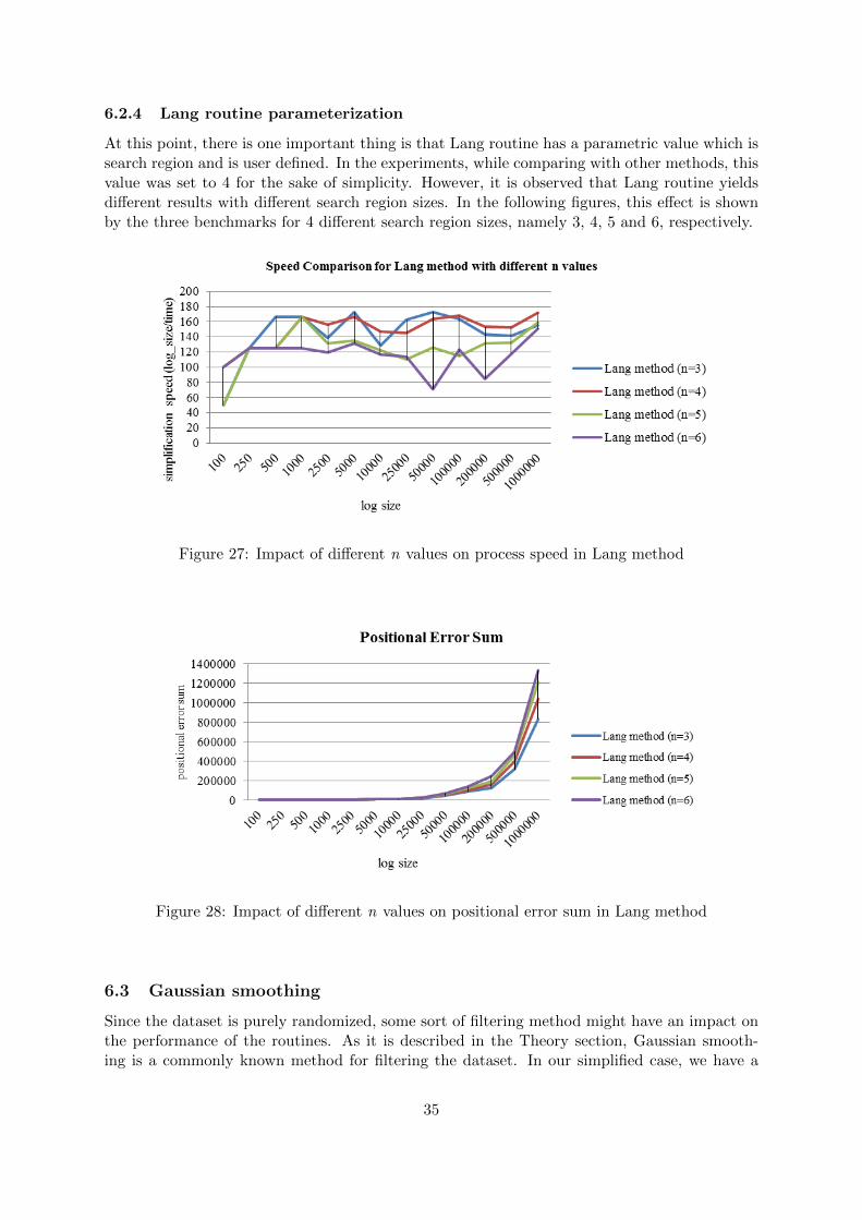
At this point, there is one important thing is that Lang routine has a parametric value which issearch region and is user defined. In the experiments, while comparing with other methods, thisvalue was set to 4 for the sake of simplicity. However, it is observed that Lang routine yieldsdifferent results with different search region sizes. In the following figures, this effect is shownby the three benchmarks for 4 different search region sizes, namely 3, 4, 5 and 6, respectively.

Figure 27: Impact of different n values on process speed in Lang method

Figure 28: Impact of different n values on positional error sum in Lang method

6.3 Gaussian smoothing

Since the dataset is purely randomized, some sort of filtering method might have an impact onthe performance of the routines. As it is described in the Theory section, Gaussian smooth-ing is a commonly known method for filtering the dataset. In our simplified case, we have a

35

Figure 29: Impact of different n values on total areal difference in Lang method

1-dimensional dataset with randomized values. The idea behind using the Gaussian smoothingis to have a preprocessing by filtering the dataset so that we could have a smoother line withthe same characteristics as the original polyline, but having a faster and more accurate sim-plification process. The emerged results are thought to be interesting enough to be consideredfor using as a preprocessing method for simplification. Since using filtering as preprocessingmethod yields slightly different results, it is decided to be given at a different section than theother results.

In order to see how Gaussian smoothing is used as a preprocessing process, Figure 30 can beobserved. The black line denotes the original polyline, the yellow line is the filtered version ofthe original polyline where σ = 0.70 and the red line represents the simplified version of filteredpolyline. It can be seen that local maximum and minimum points of the original polylineare shifted upwards and downwards due to the filtering effect, however, the global curvaturecharacteristics of the original polyline line is retained.

Figure 30: 50-point polyline filtered and then simplified (σ = 0.75) by using Douglas-Peuckerroutine

Determination of σ value

In order to determine which σ value to be used, I have performed an experiment to check thepositional error sum and total areal error sum wih different values of σ value for fixed datasetsize and also compared the time of the filtering process. The results for the distance measure

36

for different values of σ are given in Figure 31. As it is seen on the figure, a σ value around 0.7is yielding the lowest error in the results.

(a) Comparison of different σ values on totalareal error for 1000 dataset size

(b) Comparison of different σ values on positionalerror sum for 1000 dataset size

Figure 31: Determination of σ value according to the distance measure

Apart from the error measurements, time needed for the filtering is also measured. Accordingto the nature of Gaussian kernel filtering, for σ = 1, the dataset size is reduced by the factorof 2. (Refer to the Gaussian smoothing description, dataset size after smoothing = (originaldataset size / 2σ)). Therefore, there’s a drastic change for the filtration time for integer valuesof 2σ (i.e. when σ = 1, 1.5, 2, 2.5 etc.). However, increasing σ value to greater value than 1causes a drastic increase in the error measurements. For this reason, σ value is decided to betaken as 0.7 in the experiments.

Impact of Gaussian smoothing on performance - Process speed

In order to have a sound comparison, preprocessing method is used to filter the dataset and thefiltered dataset is simplified by using each implemented simplification routines. It is observedthat simplification speed is actually increasing on when it is used with Douglas-Peucker routine.In all other routines, preprocessing yields lower speeds than the non-filtered processes. In Figure32, the impact of filtering on the performance of Douglas-Peucker can be seen. The importantoutcome of this find is that Douglas-Peucker routine is yielding the most accurate simplifiedoutput compared to other existing routines and the biggest known drawback of the routine isthe very low-speed. [16] Here is an opportunity area to increase the process speed by usingfiltration.

Impact of Gaussian smoothing on performance - Reduction rate

After comparing the process speed, the impact of filtering on the reduction rates are investigated.Filtering has an obvious impact on the reduction rates of all simplification routines. Theexperiments showed that reduction rates of all simplification routines except for nth-Pointroutine are increased, as can be seen on Figure 33. The reason of no change in nth-Pointroutine is simple; the number of points after filtration is not changed unless the σ is not greaterthan 1, in the experiments, σ = 0.7.

Latter to the individual comparison, reduction rates of all the methods are compared andit is observed that Douglas-Peucker routine achieves the highest amount of reduction rate per-centages in all dataset sizes, compared to the other simplification routines.

37

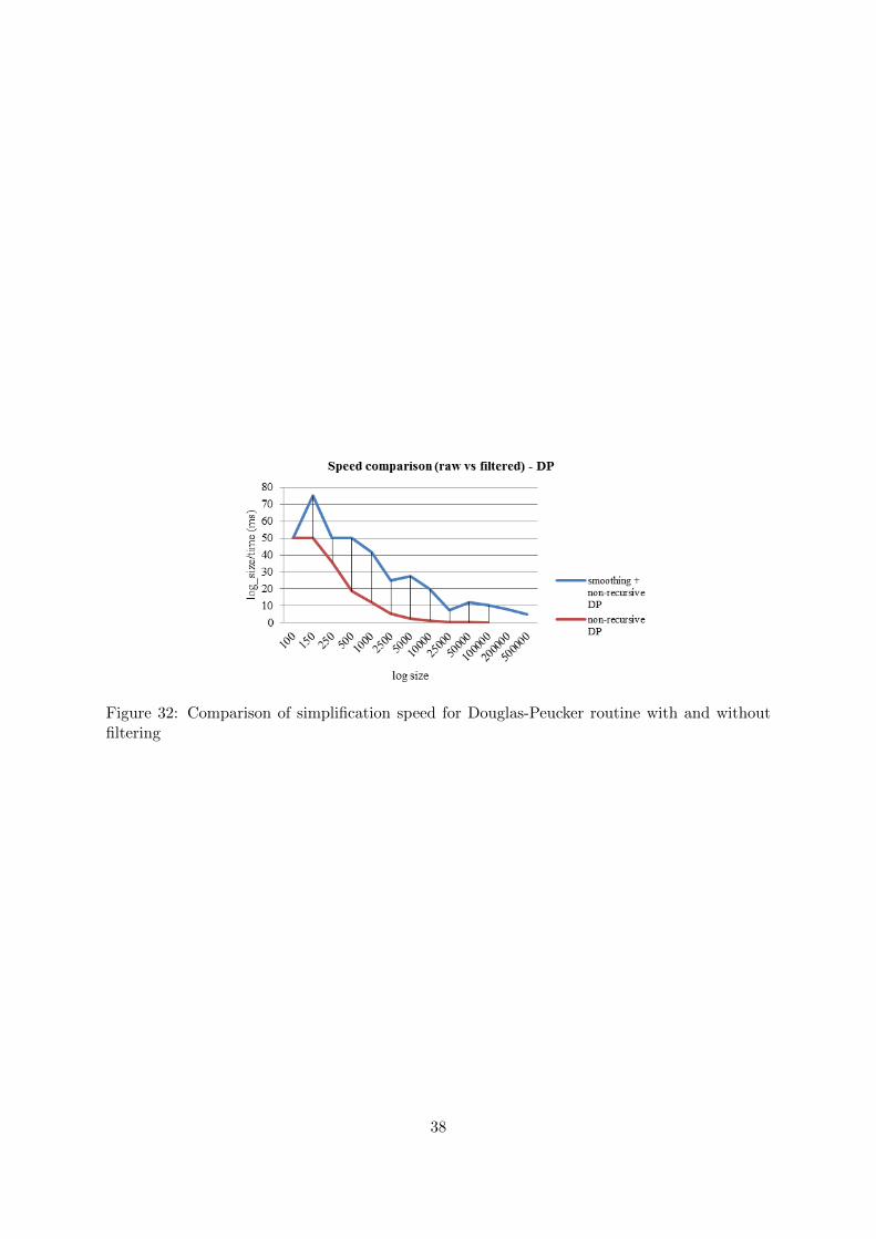
Figure 32: Comparison of simplification speed for Douglas-Peucker routine with and withoutfiltering

38

(a) reduction rate comparison for Douglas-Peucker rou-tine, filtered vs non-filtered dataset

(b) reduction rate comparison for nthPoint routine,filtered vs non-filtered dataset

(c) reduction rate comparison for Lang routine, fil-tered vs non-filtered dataset

(d) reduction rate comparison for Reumann-Witkamroutine, filtered vs non-filtered dataset

(e) reduction rate comparison for triangular rou-tine, filtered vs non-filtered dataset

Figure 33: Comparison of reduction rates for each simplification routines with and withoutfiltering

39

Impact of Gaussian smoothing on performance - Dissimilarity Measure

When using filtration as a preprocessing step, filtering the original dataset leaves offset whichcauses a high amount of positional displacement. So, looking at the positional error sum whileevaluating the impact of filtering is not meaningful. For this reason, dissimilarity measure isdone by calculating the total areas under the original and filtered and simplified polylines byusing Simpsons rule. One crucial finding was that, total areal error was lowered in all thesimplification routines when filtration is used. Figure 34 shows the total areal error of allsimplification methods with and without smoothing used as a preprocessing. On the mutipleplot, the effect of filtration on total areal error can be seen very easily. The number units for thetotal areal error are calculated by assuming all the units are in meters. More important thanunits, relative comparison of the total areal errors are deemed more important. The impactof filtration can be seen that all simplification routines are having less total areal error whensmoothing is used as preprocessing. It is observed that triangular method with smoothing aspreprocessing yields the lowest total areal error. After that, smoothing with Reumann-Witkamroutine yields the lowest areal error and after that Lang routine (with search region = 5) andDouglas-Peucker routines are filling up.

Figure 34: Comparison of total areal errors for all simplification routines with and withoutfiltering

Overall comparison

After performing all the evaluations, the performance evaluation results are observed and in or-der to put everything together, following table is generated. Table 4 represents the performanceevaluation of the simplification methods as stars, more stars mean to have a positive effect onthat side. To have the overview, total number of stars are enumerated in Total column.

40

Table 4: Overall comparison of the simplification algorithms according to 4 criteria, which areperformance (speed), shape distortion (positional error sum), visual difference (total areal sum)and rendering speed (reduction rate)

Simplificationroutine

Performance(speed)

Shapedistortion(PositionalError Sum)

VisualDifference

(Total ArealSum)

RenderingSpeed

(Reductionrate)

Total

Douglas-Peucker * *** *** **** 11Lang ** *** * *** 8

Reumann-Witkam *** * **** *** 11nth point **** ** ** ** 10

Triangular area *** **** *** * 11

41

7 Discussion & Conclusions

The pursued goal in this project has been to implement and analyze the existing simplificationroutines on large datasets and determine the usability of each simplification method and toobtain a comprehensive performance analysis of each routine.

In order to achieve this purpose, a series of datasets are generated and impact of simplifica-tion routines on these datasets are being evaluated. While generating the datasets, the inputfrom the company was stating that there was a lot of fluctuations in the data points they obtainfrom the clients, and simplification was needed to be applied on those noise-dominant regions,therefore datasets are generated as random coordinate pairs, varying between 10 and 20 meters.Datasets have varying sizes from 100 to 1 000 000 data points. After implementing the randomdataset generator, instead of working on Schlumberger’s Petrel, I decided to create my ownframework and perform the experiments on it. The main reason for that was that the sourcecode Petrel was having an huge size and dependencies among the internal classes, so that aminor change in the specific parts of the code would cause unpredictable results in the overallprocess. Furthermore, what has been developed in my own framework are totally Petrel ori-ented so that the code pieces from my framework could be very easily plugged into Petrel’sframework. After achieving the performance evaluations, all the code is tested on Petrel andis proven to work smoothly.

Although the coordinates are being generated in 3D space, it is narrowed down to 2D spacein order to focus only on polyline simplification. At that point, the main approach of the projectstood in between two different areas; digital cartography and level of detail (LOD) approach.Polyline simplification is the major interest of digital cartography, however, in cartography thedataset sizes are relatively smaller than as of they are in LOD approach. In cartography, most ofthe polylines are circular and intersecting with themselves as they are representing a piece of aland or geographical structure from the top-view. However, in this project, non of the polylinesare circular, nor intersecting themselves in any condition. They are laying on the x-axis of thegeographical structure with incrementing values. Since the main focus of the project was onimplementing an efficient algorithm on large datasets, the knowledge and experiences from bothareas has been benefited in order the pursue the simplification process.

The first major objective of the project was to implement a robust, fail-free algorithm sothat it would work in all different sizes of datasets. In terms of robustness, a recursive algorithmalways has the potential to cause stack overflow errors with large data sizes or high amountof function calls, therefore any kind of recursion should be kept away from the routines. OnlyDouglas-Peucker routine had a recursive implementation and in order to obtain robustness, therecursive Douglas-Peucker routine has been converted into non-recursive routine by modifyingthe implementation. The performance results of each routine are checked and a very low differ-ence percentage around 1.1 % has been observed in comparison. Moreover, it is observed thatrecursive algorithm encountered a stack overflow error with the dataset sizes larger than 20 000data points.

After implementing each simplification routine, benchmarks for evaluations are determinedand several tests are performed. The evaluation benchmarks are divided into 3 subgroups; pro-cess time and speed comparison, reduction rate comparison, dissimilarity measure comparison,each of which signifies a different quality in terms of simplification. In terms of process time,Douglas-Peucker routine has yielded the highest process time, which in other words means has

42

the slowest speed in simplification process. On the other hand, nth point routine achieved thefastest process speed among the other simplification routines. The main reason for Douglas-Peucker routine to be that slow is that it is a global simplification process which means ineach step of simplification, it checks the entire piece of the sub-polyline. For that reason, thecomplexity of the routine is O(n2), therefore with the enlarging dataset size, the process speedvanishes. Oppositely, nth point routine has the fastest speed and the reason is that it is abrute-force routine, which is basically a memory allocation process, retaining only the first, lastand the nth point of the polyline after simplification. It does not guarantee any kind of shapesimilarity after the simplification and it does not consider the curvature or the overall geometryof the polyline. On the other hand, Douglas-Peucker routine is a much more sophisticatedroutine. In between Douglas-Peucker and nth point routine, there are Triangular area routine,Reumann-Witkam routine and Lang routine are laying down, respectively. Reumann-Witkamand Triangular routines have very similar process time and speed results, whereas Lang routineachieved a lower result than them.

Second important benchmark is the reduction rate, which basically means the number ofthe remaining points after the simplification, and has a direct relationship with the renderingspeed. In terms of reduction rate, Douglas-Peucker routine has achieved the highest amount ofreduction rate, whereas the triangular area routine yielded a very poor reduction rate, around32% of value. The other remaining routines achieved similar reduction rates to each other.Douglas-Peucker routine achieved such a high amount of reduction rate mainly due to its so-phisticated searching algorithm for the crucial peak points and omitting all the other minorchanges on the entire polyline set [?]. Douglas-Peucker yields this highest amount of reductionwith the cost of really long process time. It can be considered as the trade-off between theprocess time and reduction rate (or rendering time), we might need a high amount of accuratereduction but if takes more than 2 minutes, it might not be a feasible option to use it.

Another important quality criteria is the dissimilarity measure, which is also very importantfor determining the visual perceptional quality of the simplification. As McMaster stated earlier[9], there should be two different groups for quantifying the dissimilarity measure, one of whichis the positional error and the other one is the areal displacement measure. Positional errorsum basically means the positional difference of each vertex on the original polyline from itssimplified version. It is a cumulative value, where it reflects how much of the shape is distortedor not. The overall comparison of each method showed that triangular area routine yields theleast amount of positional error sum, mainly because of the fact that it performs a very detailedsearch considering each 3 successive vertices of the polyline while processing the simplification.On the other hand, Reumann-Witkam routine yields the highest amount of positional errorsum. Nth point follows it by the second highest amount of error summation. Douglas-Peuckerroutine has the second lowest cumulative positional error. Here comes an important question,does the fact Reumann-Witkam routine yields the highest positional error sum mean that ityields the worst visual perceptional quality? In order to answer this question, the total arealdisplacement has to be evaluated and compared. Because during the simplification method,the simplification routine might cause a lot of shape distortions but it might retain the globalcharacteristics of the polyline, which is also an important criteria. While evaluating the totalareal displacement, the areas under the original and the simplified polylines are calculated andthe difference is deemed as the areal error of the simplification. It is observed that Lang methodachieved the highest total areal displacement after the simplification, which means the overallshape of the simplified polyline has changed the most when Lang method is used. On the otherhand, Reumann-Witkam routine, which yielded the highest positional error sum in the compar-

43

ison, yielded one of the least amount of total areal displacement in between the original and thesimplified polylines. Reumann-Witkam, Douglas-Peucker and triangular area routine yieldedvery similar and relative low total areal errors, where Douglas-Peucker routine was observed tohave a more robust areal error displacement, compared to the other 2 routines.

As an overall picture at this point, it has been remarked that each simplification routinehas a different advantage in different aspect. Triangular areal method is achieving a really lowpositonal and areal error sum with an acceptable process speed, whereas it yields a very lowreduction rate which yields a long rendering time after simplification. On the other hand, amathematical superior, Douglas-Peucker routine yields quite good results in dissimilarity mea-sures and reduction rate, whereas it yields the slowest process speed for the simplification. Twomethods which are having similar principles, Lang and Reumann-Witkam routines yield veryclose results to each other in many performance criteria, except for the total areal displace-ment. Reumann-Witkam routine yields a lower total areal displacement than Lang routinewhich means that Reumann-Witkam routine is better at preserving global characteristics of thepolyline.

After comparing each simplification routines’ performances, a new idea as preprocessing stepis implemented: filtering, or smoothing algorithm. The main concern for the smoothing processis to reduce the noise in the original polyline so that it can get easier and faster to performsimplification routines. As an initial trial, Gaussian smoothing kernel is used with varying σvalues. Three different σ values are tested, from 0.5 to 1 and σ value of 0.70 is selected to beused for smoothing processes, as it yielded a very low total areal error after smoothing process.Employing smoothing process at the beginning of the simplification, and then applying the sim-plification routines, indeed had an interesting impact on the performance results. First of all,the process speed of Douglas-Peucker routine has increased drastically whereas for all the otherroutines, using smoothing as preprocessing caused lower process speeds. This is an importantfinding as the main disadvantage of Douglas-Peucker routine was its slow speed. Apart from theprocess time comparison, reduction rates of each method is compared with and without usingsmoothing process, and as expected, it was observed that all the reduction rates are increasedwhen smoothing is used. This is expected because smoothing process already reduces the noisewithin the original polyline therefore the reduction rate results after the simplification are lower.An important outcome of this is that triangular area routine, which yields the lowest reductionrate 32% could achieve a reduction rate of 50%.

The effect of smoothing in terms of dissimilarity measure could only be quantified for thetotal areal error sum. It was not feasible to check the positional error sum as smoothing processchanges the coordinates of all the points, therefore very high positional error would be observed.However, this does not mean that the smoothing process causes a very different visual percep-tion, as it retains the curvature details of the original polyline. Therefore, the total areal errorresults are taken into account while evaluating the effect of smoothing. When all the results areput on one plot, in Figure 34, it is observed that all the routines yield lower areal error sumswhen the smoothing used as a preprocessing speed. Among the ones with smoothing process,triangular area routine yielded the least areal error sum, Lang and Reumann-Witkam routinesfollowed it by the second and third least areal error sum. Looking at the big picture, it couldbe said that using smoothing algorithm as a preprocessing step had a positive impact on theperformance of all simplification routines.

To sum up all the evaluations, the reader should now be referred to the Table 4 to check

44

the overall rates of all the simplification routines that are used and tested in this project. Itis clearly seen that Douglas-Peucker, Reumann-Witkam and triangular area routines have thesame cumulative ratings in terms of performance criteria. Each of them have different strengthsand weaknesses among each other, depending on the quality criteria. It can also be concludedthat smoothing has a positive effect on the overall simplification process, except for the processtime on the simplification routines apart from Douglas-Peucker.

8 Future Work

In this project, there has been 5 simplification routines under consideration and all the evalua-tions and comparisons are done around those routines. It is known that there are other existingsimplification routines, namely Opheim algorithm, Visvalingam-Whyatt algorithm, Zhao algo-rithm and Saalfeld’s algorithm routines [6]. Many of those algorithms are developed for digitalcartography usage and not tested on large datasets. It would be interesting to implement thosealgorithms on large datasets and obtain the performance results.

Another important next step would be to work on implementing and investigating the im-provements on the speed of Douglas-Peucker simplification routine, as Douglas-Peucker routineyields quite good results in many performance criteria aspects. One important finding is that,applying a convex hull algorithm into the Douglas-Peucker routine is found to achieve fasterresults on simplification process [?]. Apart from that, it might also be an interesting approachto parallelize the simplification process, and using different processors while treating each sub-polyline. I reckon this would have a great impact on the performance of the Douglas-Peuckerroutine.

While determining the dissimilarity measure, only positional and areal error sums are eval-uated and compared, but also angular dissimilarities in between the original and simplifiedpolylines could be compared, to have a different perspective on quantifying the dissimilarity.

Interactivity is another important area since after all Petrel is a visualization toolkit whichenables the user of the tool to interact with the dataset. In terms of interactivity, FPS (framesper second) measure is an important benchmark, but more parameters could be changed inthe current status. One example would be to implement a better LOD approach, which mightbe considered as having 3 or 4 different visual qualities in the object shown on the screen,depending on the distance to the camera. In the furthest point from the user, the object couldbe simplified in the most rough but fastest way so that the visual quality would not play animportant role. As the object gets closer to the camera, it can get more and more details,by using different simplification methods. Moreover, since the main focus is on large datasets,and they are viewed on the screen with perspective, the further parts of the polyline can besimplified differently than closer parts to the camera (i.e. more simplification on further partsof the polyline).

45

9 Appendix

Positional Error Sum calculation on c++ code script:

Vector3D s im p l i f i e d f i r s t , s imp l i f i e d p r e v , s imp l i f i e d l a s t , o r i g i n a l f i r s t , o r i g i n a l l a s t ;s i m p l i f i e d f i r s t = po in t s s imp l [ 0 ] ;s i m p l i f i e d l a s t = po in t s s imp l [ num vert i ces out −1] ;o r i g i n a l f i r s t = po in t s [ 0 ] ;o r i g i n a l l a s t = po in t s [ l o g s i z e −1] ;s imp l i f i e d p r e v = s i m p l i f i e d f i r s t ;s i m p l i f i e d f i r s t = po in t s s imp l [ 1 ] ;

int kk=0;int mm=0;while ( s i m p l i f i e d f i r s t . operator ==(s im p l i f i e d l a s t ) == fa l se ){

while ( o r i g i n a l f i r s t . operator == ( o r i g i n a l l a s t ) == fa l se && ( o r i g i n a l f i r s t . operator == ( s i m p l i f i e d f i r s t )==fa l se ) ) {r e s u l t += minDistance ( s imp l i f i e d p r e v , s i m p l i f i e d f i r s t , o r i g i n a l f i r s t ) ;kk++;o r i g i n a l f i r s t = po in t s [ kk ] ;

}s imp l i f i e d p r e v = s i m p l i f i e d f i r s t ;mm++;s i m p l i f i e d f i r s t = po in t s s imp l [mm+1] ;}

}

Total Areal Sum calculation by Trapezoidal method in between the original and simplifiedpolyline c++ code script:

double sumTrapezoidal org = 0 . 0 ;double sumTrapezoidal s impl = 0 . 0 ;double s umTrape zo i da l s imp l f i l t = 0 . 0 ;for ( int i = 1 ; i < l o g s i z e ; i++) {

sumTrapezoidal org += ( po in t s [ i ] . x ( ) − po in t s [ i −1] . x ( ) ) ∗ ( po in t s [ i ] . y()+ po in t s [ i −1] . y ( ) ) ;}sumTrapezoidal org = sumTrapezoidal org ∗ 0 . 5 ;

for ( int i = 1 ; i < num ver t i c e s out ; i++) {sumTrapezoidal s impl += ( po in t s [ o u t i n d i c e s [ i ] ] . x ( ) − po in t s [ o u t i n d i c e s [ i −1 ] ] . x ( ) ) ∗ ( po in t s [ o u t i n d i c e s [ i ] ] . y()+ po in t s [ o u t i n d i c e s [ i −1 ] ] . y ( ) ) ;

}sumTrapezoidal s impl = sumTrapezoidal s impl ∗ 0 . 5 ;

for ( int i = 1 ; i < num v e r t i c e s o u t f i l t ; i++) {s umTrape zo i da l s imp l f i l t += ( samp l e sF i l t e r ed [ o u t i n d i c e s f i l t e r e d [ i ] ] . x ( ) − s amp l e sF i l t e r ed [ o u t i n d i c e s f i l t e r e d [ i −1 ] ] . x ( ) ) ∗ ( s amp l e sF i l t e r ed [ o u t i n d i c e s f i l t e r e d [ i ] ] . y()+ samp l e sF i l t e r ed [ o u t i n d i c e s f i l t e r e d [ i −1 ] ] . y ( ) ) ;

}s umTrape zo i da l s imp l f i l t = sumTrape zo i da l s imp l f i l t ∗ 0 . 5 ;

double e r r o r a r e a l t r a p e z o i d a l = abs ( sumTrapezoidal org−sumTrapezoidal s impl ) ;}

Total Areal Sum calculation by Simpson’s method in between the original and simplified polylinec++ code script:

double sumSimpsons org = 0 . 0 ;double sumSimpsons simpl = 0 . 0 ;double sumSimpsons f i l t = 0 . 0 ;double sumSimpsons f i l t s imp l = 0 . 0 ;for ( int i = 1 ; i < l o g s i z e ; i++) {

sumSimpsons org += ( po in t s [ i ] . x ( ) − po in t s [ i −1] . x ( ) ) ∗ ( po in t s [ i −1] . y ( ) + 4 ∗ ( po in t s [ i ] . y ( ) + po in t s [ i −1] . y ( ) ) / 2 + po in t s [ i ] . y ( ) ) ;}sumSimpsons org = sumSimpsons org ∗ 1/6 ;

for ( int i = 1 ; i < num ver t i c e s out ; i++) {sumSimpsons simpl += ( po in t s [ o u t i n d i c e s [ i ] ] . x ( ) − po in t s [ o u t i n d i c e s [ i −1 ] ] . x ( ) ) ∗ ( po in t s [ o u t i n d i c e s [ i −1 ] ] . y ( ) + 4 ∗ ( po in t s [ o u t i n d i c e s [ i −1 ] ] . y ( ) + po in t s [ o u t i n d i c e s [ i ] ] . y ( ) ) / 2 + po in t s [ o u t i n d i c e s [ i ] ] . y ( ) ) ;

}sumSimpsons simpl = sumSimpsons simpl ∗ 1/6 ;

for ( int i = 1 ; i < newSize ; i++) {sumSimpsons f i l t += ( samp l e sF i l t e r ed [ i ] . x ( ) − s amp l e sF i l t e r ed [ i −1] . x ( ) ) ∗ ( s amp l e sF i l t e r ed [ i −1] . y ( ) + 4 ∗ ( s amp l e sF i l t e r ed [ i ] . y ( ) + samp l e sF i l t e r ed [ i −1] . y ( ) ) / 2 + samp l e sF i l t e r ed [ i ] . y ( ) ) ;

}

46

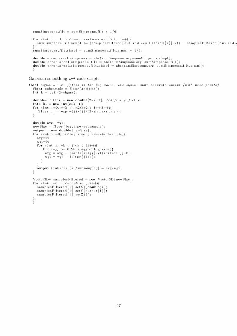
sumSimpsons f i l t = sumSimpsons f i l t ∗ 1/6 ;

for ( int i = 1 ; i < num v e r t i c e s o u t f i l t ; i++) {sumS impsons f i l t s imp l += ( samp l e sF i l t e r ed [ o u t i n d i c e s f i l t e r e d [ i ] ] . x ( ) − s amp l e sF i l t e r ed [ o u t i n d i c e s f i l t e r e d [ i −1 ] ] . x ( ) ) ∗ ( s amp l e sF i l t e r ed [ o u t i n d i c e s f i l t e r e d [ i −1 ] ] . y ( ) + 4 ∗ ( s amp l e sF i l t e r ed [ o u t i n d i c e s f i l t e r e d [ i −1 ] ] . y ( ) + samp l e sF i l t e r ed [ o u t i n d i c e s f i l t e r e d [ i ] ] . y ( ) ) / 2 + samp l e sF i l t e r ed [ o u t i n d i c e s f i l t e r e d [ i ] ] . y ( ) ) ;

}sumS impsons f i l t s imp l = sumSimpsons f i l t s imp l ∗ 1/6 ;

double e r r o r a r e a l s imp s on s = abs ( sumSimpsons org−sumSimpsons simpl ) ;double e r r o r a r e a l s i m p s o n s f i l t = abs ( sumSimpsons org−sumSimpsons f i l t ) ;double e r r o r a r e a l s imp s o n s f i l t s im p l = abs ( sumSimpsons org−sumSimpsons f i l t s imp l ) ;}

Gaussian smoothing c++ code script:

f loat sigma = 0 . 8 ; // t h i s i s the key va lue . low sigma , more accurate output ( with more po in t s )f loat subsample = f l o o r (2∗ sigma ) ;int k = c e i l (2∗ sigma ) ;

double∗ f i l t e r = new double [ 2∗ k+1] ; // de f i n i n g f i l t e rint∗ k = new int [ 2∗ k+1] ;for ( int i =0, j=−k ; i<2∗k+2 ; i++, j++){

f i l t e r [ i ] = exp(−( j )∗ ( j )/(2∗ sigma∗ sigma ) ) ;}

double avg , wgt ;newSize = f l o o r ( l o g s i z e / subsample ) ;output = new double [ newSize ] ;for ( int i i =0; i i < l o g s i z e ; i i= i i+subsample ){

avg=0;wgt=0;for ( int j j=−k ; j j<k ; j j ++){

i f ( i i+j j >= 0 && i i+j j < l o g s i z e ){avg = avg + po in t s [ i i+j j ] . y ( )∗ f i l t e r [ j j+k ] ;wgt = wgt + f i l t e r [ j j+k ] ;

}}output [ ( int ) c e i l ( i i / subsample ) ] = avg/wgt ;

}

Vector3D∗ s amp l e sF i l t e r ed = new Vector3D [ newSize ] ;for ( int i=0 ; i<=newSize ; i++){

s amp l e sF i l t e r ed [ i ] . setX ( (double ) i ) ;s amp l e sF i l t e r ed [ i ] . setY ( output [ i ] ) ;s amp l e sF i l t e r ed [ i ] . setZ ( 1 ) ;

}}

47