Embed Size (px)
Citation preview
HAL Id: inria-00181445https://hal.inria.fr/inria-00181445
Submitted on 24 Oct 2007
HAL is a multi-disciplinary open accessarchive for the deposit and dissemination of sci-entific research documents, whether they are pub-lished or not. The documents may come fromteaching and research institutions in France orabroad, or from public or private research centers.
L’archive ouverte pluridisciplinaire HAL, estdestinée au dépôt et à la diffusion de documentsscientifiques de niveau recherche, publiés ou non,émanant des établissements d’enseignement et derecherche français ou étrangers, des laboratoirespublics ou privés.
Efficient GPU-based Construction of Occupancy GridsUsing several Laser Range-finders
Manuel Yguel, Olivier Aycard, Christian Laugier
To cite this version:Manuel Yguel, Olivier Aycard, Christian Laugier. Efficient GPU-based Construction of OccupancyGrids Using several Laser Range-finders. International Journal Of Autonomous Vehicles, 2007, ToAppear Spring. <inria-00181445>
Efficient GPU-based Construction of OccupancyGrids Using several Laser Range-finders.
Manuel Yguel, Olivier Aycard and Christian LaugierINRIA Rhone-Alpes,
Grenoble, Franceemail: [email protected]
Abstract— Building occupancy grids (OGs) in order to modelthe surrounding environment of a vehicle implies to fusion occu-pancy information provided by the different embedded sensors inthe same grid. The principal difficulty comes from the fact thateach can have a different resolution, but also that the resolutionof some sensors varies with the location in the field of view. Inthis article we present a new efficient approach to this issuebasedupon a graphical processor unit (GPU). In that perspective,weexplain why the problem of switching coordinate systems is aninstance of the texture mapping problem in computer graphics.We also present an exact algorithm in order to evaluate theaccuracy of such a device, which is not precisely known due tothe several approximations made by the hardware. To validateour method, the results with GPU are also compared to resultsobtained through the exact approach and the GPU precisionis shown to be good enough for robotic applications. Thereforewe describe a whole and general calculus architecture to buildoccupancy grids for any kind of range-finder with a graphicalprocessor unit (GPU). And we present computational time resultsthat can allow to compute occupancy grids for 50 sensors at framerate even for a very fine grid.
I. I NTRODUCTION
At the end of the 1980s, Elfes and Moravec introduceda new framework to multi-sensor fusion called occupancygrids (OGs). An OG is a stochastic tessellated representationof spatial information that maintains probabilistic estimatesof the occupancy state of each cell in a lattice [1]. Inthis framework, each cell is considered separately for eachsensor measurement, and the only difference between cellsis the position in the grid. For most common robotic tasks,the simplicity of the grid-based representation is essential,allowing robust scan matching [2], accurate localizationand mapping [3], efficient path planning algorithms [4] andocclusion handling for multiple target-tracking algorithms [5].The main advantage of this approach is the ability to integrateseveral sensors in the same framework, taking the inherentuncertainty of each sensor reading into account, contraryto the Geometric Paradigm[1], a method that categorizesthe world features into a set of geometric primitives. Themajor drawback of the geometric approach is the numberof different data structures for each geometric primitivethat the mapping system must handle: segments, polygons,ellipses, etc. Taking into account the uncertainty of the sensormeasurements for each sequence of different primitives isvery complex, whereas the cell-based framework is genericand therefore can fit every kind of shape and be used to
interpret any kind and any number of sensors. Moreover, OGsallow easily the combination of redundant sensors that limitsthe effects of sensor breakdown and enlarges the robot fieldof view.
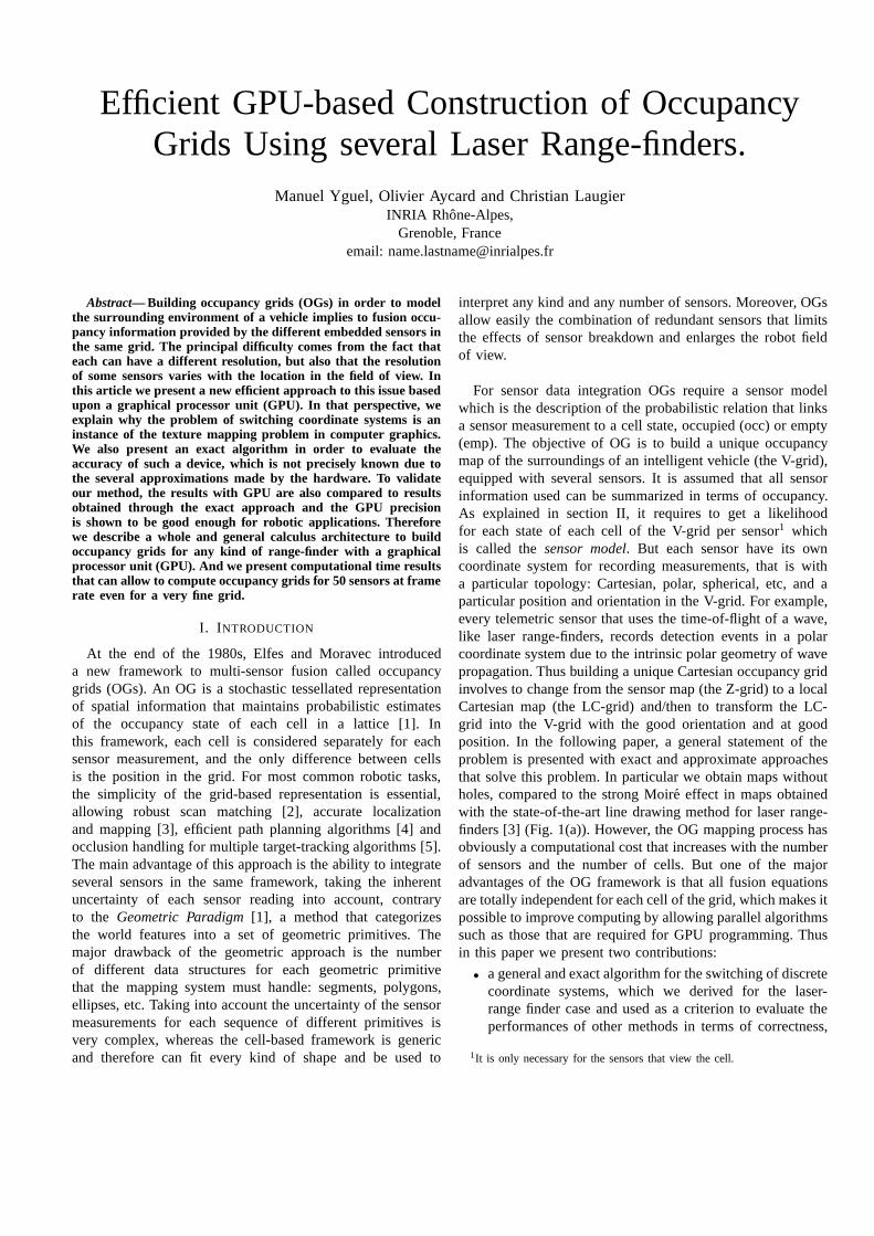
For sensor data integration OGs require a sensor modelwhich is the description of the probabilistic relation thatlinksa sensor measurement to a cell state, occupied (occ) or empty(emp). The objective of OG is to build a unique occupancymap of the surroundings of an intelligent vehicle (the V-grid),equipped with several sensors. It is assumed that all sensorinformation used can be summarized in terms of occupancy.As explained in section II, it requires to get a likelihoodfor each state of each cell of the V-grid per sensor1 whichis called thesensor model. But each sensor have its owncoordinate system for recording measurements, that is witha particular topology: Cartesian, polar, spherical, etc, and aparticular position and orientation in the V-grid. For example,every telemetric sensor that uses the time-of-flight of a wave,like laser range-finders, records detection events in a polarcoordinate system due to the intrinsic polar geometry of wavepropagation. Thus building a unique Cartesian occupancy gridinvolves to change from the sensor map (the Z-grid) to a localCartesian map (the LC-grid) and/then to transform the LC-grid into the V-grid with the good orientation and at goodposition. In the following paper, a general statement of theproblem is presented with exact and approximate approachesthat solve this problem. In particular we obtain maps withoutholes, compared to the strong Moire effect in maps obtainedwith the state-of-the-art line drawing method for laser range-finders [3] (Fig. 1(a)). However, the OG mapping process hasobviously a computational cost that increases with the numberof sensors and the number of cells. But one of the majoradvantages of the OG framework is that all fusion equationsare totally independent for each cell of the grid, which makes itpossible to improve computing by allowing parallel algorithmssuch as those that are required for GPU programming. Thusin this paper we present two contributions:
• a general and exact algorithm for the switching of discretecoordinate systems, which we derived for the laser-range finder case and used as a criterion to evaluate theperformances of other methods in terms of correctness,
1It is only necessary for the sensors that view the cell.
(a) (b)
Fig. 1. (a) 2D OG obtained by drawing lines with 1D occupancy mapping (for a SICK laser-range finder). The consequences area Moire effect (artificialdiscontinuities between rays far from origin). (b) 2D OG obtained from the exact algorithm. All the OGs are 60m× 30m with a cell side of 5cm,i.e. 720000cells.
precision and computing advantages.• a very efficient GPU implementation of multi-sensor
fusion for occupancy grids including the switch of co-ordinate systems validated by the results of the previousmethod.
In the conclusions of the first study we demonstrate theequivalence between the occupancy grid sensor fusion and thetexture mapping problem in computer graphics [6]. And inthe second contribution, we use the parallel texture mappingcapabilities of GPU, to obtain a fast procedure of fusion andcoordinate system switch. Thus, the experiments show thatGPU allows to produce occupancy grid fusion for 50 sensorssimultaneously at sensor measurement rate.
The paper is organized as follows: we present first math-ematical equations of sensor fusion and the 1D equations oftelemetric sensor model we use. Then we focus on the switchof coordinate systems from polar to Cartesian because formost telemetric sensors the intrinsic geometry is polar. Thenwe explain how to simplify the above switch of coordinatesystems to improve the computational time with parallelism,taking into account precision and/or safety. Finally in thelastsections we present our GPU-based implementation and theresults of fusion obtained for 4 sick laser range-finders withcentimetric precision.
II. SENSORFUSION IN OCCUPANCY GRIDS
A. Bayesian sensor fusion.
The general problem of sensor fusion for OG is presentedhere first for a grid cell and several sensors.
a) Probabilistic variable definitions:
•−→Z = (Z1, . . . , Zs) a vector ofs random variables2, onevariable for each sensor. We consider that each sensorican return measurements from a setZi.
• Ox,y ∈ O ≡ occ, emp. Ox,y is the state of the bin(x, y), where(x, y) ∈ Z
2.Z
2 is the set of indexes of all the cells in the monitoredarea.
2For a certain variableV we will note in capital case the variable, innormal casev one of its realization, and we will notep(v) for P ([V = v])the probability of a realization of the variable.
b) Joint probabilistic distribution: the lattice of cells isa type of Markov field and many assumptions can be madeabout the dependencies between cells and especially adjacentcells in the lattice [7]. In this article sensor models are usedfor independent cells i.e. without any dependencies, whichis a strong hypothesis but very efficient in practice since allcalculus could be made for each cell separately. It leads to thefollowing expression of a joint distribution for each cell.
P (Ox,y,−→Z ) = P (Ox,y)
s∏
i=1
P (Zi|Ox,y) (1)
Given a vector of sensor measurements−→z = (z1, . . . , zs)we apply the Bayes rule to derive the probability for cell(x, y)to be occupied:
p(ox,y|−→z ) =
p(ox,y)∏s
i=1 p(zi|ox,y)
p(occ)∏s
i=1 p(zi|occ) + p(emp)∏s
i=1 p(zi|emp)(2)
For each sensori, the two conditional distributionsP (Zi|occ) and P (Zi|emp) must be specified. This is calledthe sensor modeldefinition.
B. General form of telemetric sensor model
For the 1D-case, the sensor models, used here (eq. (7),(8)),are based upon the Elfes and Moravec Bayesian telemetricsensor models [1]. Now, is presented our own demonstration ofthe results of [1], which add a complete formalism to expressthe dependency of the sensor model on the initial occupancyof the grid cells. This initial hypothesis is called theprior.
The whole presentation is based upon the assumption thatthe telemetric sensor is of a time-of-flight type. This is anactive kind of sensor which basically emits a signal with afixed velocityv at timet0, then receives the echo of this signalat time t1, and then computes the distance of the obstaclesfrom the source with:d = t1−t0
v. We callΩ the source location
of the emitted signal.First, we consider an ideal case: when there are severalobstacles in the visibility area, only the first one (in termsof time of flight) is detected.
1) Probabilistic variable definitions:Only one sensor isconsidered.
• Z ∈ “no impact”⋃Z. Z belongs to the set of allpossible values for the sensor with the additional value:“no impact” which means that the entire scanned regionis free.
• Ox ∈ O ≡ occ, emp. ox is the state of the binxeither “occupied” or “empty”, wherex ∈ [[1; N ]]. N isthe number of cells in the 1D visibility area for a singlesensor shot.
• Gx ∈ Gx ≡ occ, emp[[1;N ]]\x. gx represents astate of all the cells in the visibility area except thex one. Gx takes its values in the t-uples of cells(c1 = o1, . . . , cx−1 = ox−1, cx+1 = ox+1, . . . , cN = oN )whereci is the celli (fig. 2).
2) Joint distributions: The probabilistic distribution de-scribing the interaction between sensor values and a cell stateis, following an exact Bayes decomposition:
P (Z, Ox, Gx) = P (Ox)P (Gx|Ox)P (Z|Gx, Ox)
• P (Ox) is the prior: this is the probability that in a celllies a surface that is reflective for the telemetric sensorused. In this case the cell is called occupied. We notethe probability that a cell contains no reflective surface(empty):u.
• P (Gx|Ox) is the probability that, knowing the state of acell, the whole visibility area is in a particular state. Here,we make a strong assumption: we assume that the stateof the cellx is non informative for the states of the othercells. So formally:P (Gx|Ox) ≡ P (Gx). However notany hypothesis about the probability of some particularstate ofGx is made. Then: the sole hypothesis is thatP (Gx) only depends on the number of empty or occupiedcells3.
• P (Z|Ox, Gx) depends of the sensor, but for all(ox, gx) ∈[[1; N ]]×Gx, the distribution overZ depends only of thefirst occupied cell. Then we suppose that knowing theposition of the first occupied cellck in the sensor viewgx, P (Z|ox, gx) behaves as if there were onlyck occupiedin all the area. We call this particular distribution overZ:the elementary sensor modelPk(Z).
To computeP (Z, Ox) we derive, now, equations for themarginalization over all the possible states ofGx.
3) Inference :To avoid the numerical pitfall of consideringall the possible cell states ofGx, an inference calculus isdone here based upon a marginalization sum. The heart of thesolution to the inference problem is to deal with the visibilityof a bin. Considering a perfect case, the first occupied cellin the visibility area causes a detection. So knowing that thecell x is occupied, that cell is the last one which can cause adetection.Therefore we give the next definition.
3which is a more general modeling than the uniform choice madein [1].
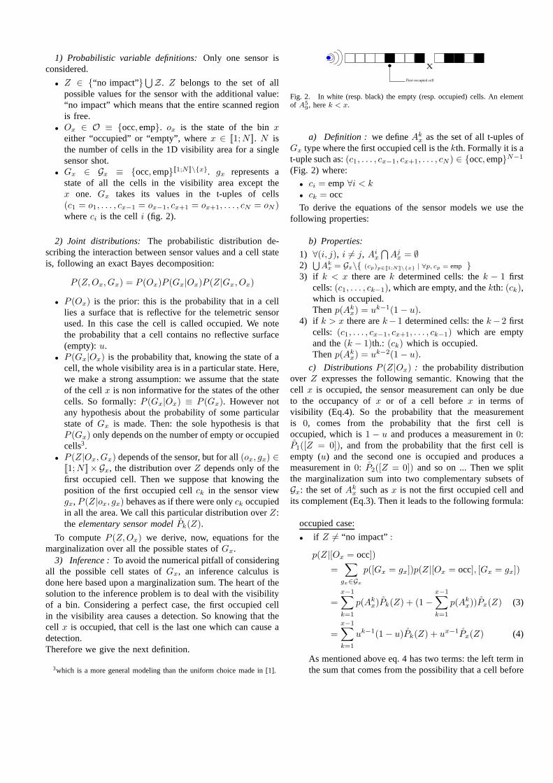
First occupied cell
X
Fig. 2. In white (resp. black) the empty (resp. occupied) cells. An elementof A5
9, herek < x.
a) Definition : we defineAkx as the set of all t-uples of
Gx type where the first occupied cell is thekth. Formally it is at-uple such as:(c1, . . . , cx−1, cx+1, . . . , cN ) ∈ occ, empN−1
(Fig. 2) where:
• ci = emp∀i < k• ck = occ
To derive the equations of the sensor models we use thefollowing properties:
b) Properties:
1) ∀(i, j), i 6= j, Aix
⋂
Ajx = ∅
2)S
Akx = Gx\ (cp)p∈[[1;N ]]\x | ∀p, cp = emp
3) if k < x there arek determined cells: thek − 1 firstcells:(c1, . . . , ck−1), which are empty, and thekth: (ck),which is occupied.Thenp(Ak
x) = uk−1(1− u).4) if k > x there arek− 1 determined cells: thek− 2 first
cells: (c1, . . . , cx−1, cx+1, . . . , ck−1) which are emptyand the(k − 1)th.: (ck) which is occupied.Thenp(Ak
x) = uk−2(1− u).
c) DistributionsP (Z|Ox) : the probability distributionover Z expresses the following semantic. Knowing that thecell x is occupied, the sensor measurement can only be dueto the occupancy ofx or of a cell beforex in terms ofvisibility (Eq.4). So the probability that the measurementis 0, comes from the probability that the first cell isoccupied, which is1 − u and produces a measurement in0:P1([Z = 0]), and from the probability that the first cell isempty (u) and the second one is occupied and produces ameasurement in0: P2([Z = 0]) and so on ... Then we splitthe marginalization sum into two complementary subsets ofGx: the set ofAk
x such asx is not the first occupied cell andits complement (Eq.3). Then it leads to the following formula:
occupied case:
• if Z 6= “no impact” :
p(Z|[Ox = occ])
=∑
gx∈Gx
p([Gx = gx])p(Z|[Ox = occ], [Gx = gx])
=x−1∑
k=1
p(Akx)Pk(Z) + (1−
x−1∑
k=1
p(Akx))Px(Z) (3)
=
x−1∑
k=1
uk−1(1− u)Pk(Z) + ux−1Px(Z) (4)
As mentioned above eq. 4 has two terms: the left term inthe sum that comes from the possibility that a cell before
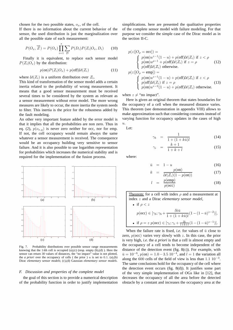
x is occupied and the right term that comes from theaggregation of all the remaining probabilities around thelast possible cell that can produce a detection event:x. Inthe case of a Diracelementary sensor model, the precisionis perfect and the aggregation is completed atx fig. 7(a).The “no impact” case ensures that the distribution isnormalized.
• if Z = “no impact”:p([Z = ”no impact”]|[Ox = occ])= 1−∑
r 6=”no impact” p([Z = r]|[Ox = occ])
empty case:
•if Z 6= “no impact” :we note open= (cp)p∈[[1;N ]]\x | ∀p, cp = emp
p(Z|[Ox = emp]) (5)
=∑
gx∈Gx
p([Gx = gx])p(Z|[Ox = emp], [Gx = gx])
=N
∑
k=1,k 6=x
p(Akx)Pk(Z) + p(open)δZ=”no impact”
=
x−1∑
k=1
uk−1(1 − u)Pk(Z)
+n
∑
k=x+1
uk−2(1− u)Px(Z) + un−1δZ=”no impact”(6)
There are three terms in the empty case: before theimpact, after and the term “no impact”. What is veryinteresting is that in both occupied and empty model theterm before impact (left term) is exactly the same fig. 7(a)and fig. 7(b). As above, the “no impact” case ensures thatevery case is considered.
• if Z = “no impact”:p([Z = ”no impact”]|[Ox = emp])= 1− (
∑
r p([Z = r]|[Ox = emp])) + uN−1δZ=”no impact”
4) Numerical models:The information to handle to define theelementary sensormodelare:
• the range of possible values returned by the sensor whichinclude maximal and minimal sensor field of view butalso granularity of the measures;
• the precision or uncertainty of a sensor measure whichcan varies with the obstacle distance for example. Whena range sensor measures the distance to an obstacle overtime, it records different measures due to the sensor ownuncertainty. For an acceptable sensor, all the records arein the close surroundings of the real obstacle distance.The probability distribution of those records defines theelementary sensor model.
The first kind of information is provided in the technicalmanuals of sensors whereas the second is often only partiallydescribed, therefore full equations are given here.
a) Dirac model: when the sensor is ideal or has astandard deviation that is far smaller than the cell size in theoccupancy grid, it is suitable to modelP (Z) with a Diracdistribution4 (Fig. 7(a)-7(b)):
Pk([Z = z]) =
1.0 if z = k0.0 otherwise.
b) Gaussian models:as all telemetric sensors are farfrom perfect, the Dirac model is obviously inappropriatein many cases. At this point the traditional choice [8]–[10]favors Gaussian distributions, centered onk and with avariance that increases withk.It models the failures of the sensor well. However in thecase of a telemetric sensor the possible values for themeasurements are always positive, but Gaussian assign nonzero probabilities to negative values. Worst, close to theorigin i.e. z = 0, this distribution assigns high values to thenegative measurements. Therefore we propose the followingdiscrete distribution based on the Gaussian5 N (µ, σ):
Pk([Z = z]) =
if z ∈ [0; 1] :∫
]−∞;1]N (k − 0.5, σ(k − 0.5))(u)du
if z ∈]1; n] :∫ ⌊z⌋+1
⌊z⌋ N (k − 0.5, σ(k − 0.5))(u)du
if z =”no impact” :∫
]n;+∞[N (k − 0.5, σ(k − 0.5))(u)du.
Whereσ(x) is an increasing function ofx. We notice thatthe probability of “no impact” is increased by the integral ofthe Gaussian over]n; +∞], which means that all the impactsurfaces beyond the sensor field of view are not detected.
An other Gaussian-based modeling was suggested in [11],to take into account all short reflections that could drivethe echo to the signal receiver before the sensor has fin-ished transmitting. These kind of telemetric sensor lis-ten and emit by the same channel, so the sensor cannotstand in both states: receiver and emitter, at same time.Pk([Z = z]) =
if z =”no impact” :∫
]−∞;1]∪]n;+∞[N (k − 0.5, σ(k − 0.5))(u)du
else:∫ ⌊z⌋+1
⌊z⌋ N (k − 0.5, σ(k − 0.5))(u)du.
Thus, we notice that the probability of “no impact” isincreased by the integral of the Gaussian over] − ∞, 1]. Inthis two modeling, introducing the special case of “no impact”is necessary to take the missed detections into account.
4Here we suppose thatz is an integer which represents the cell index, whichthe sensor measurement corresponds to: ifz is real it is⌊z⌋ + 1.
5Here we assume thatk is the index of the cell which represents all thepoints with radial coordinate in]k − 1; k], i.e. we assume a length of1 forcell, for simplicity.
C. Discussions and model properties
the goal of this section is to underline the link betweenthe above sensor model (fig. 7) and the well known shape ofOG after a detection event (fig. 3, 4 blue curves) that showthree distinct area of occupancy: empty before the obstacle,occupied at the obstacle and unknown after the obstacle. In theprecedent section, the sensor model is defined for a certain celland for each possible sensor measurements. In opposite, hereare presented the qualitative properties of the sensor modelfrom different cells point of view but for the same sensorreading. For that purpose we consider very simple cases. Inthe Diracelementary sensor modelscase, the equations for thecell numberρ are:
p(z|[Oρ = occ]) =
uz−1(1− u) if z < ρuρ−1 if z = ρ0 otherwise.
(7)
p(z|[Oρ = emp]) =
uz−1(1− u) if z < ρ0 if z = ρuz−2(1− u) otherwise.
(8)
when z 6= “no impact” and z ≥ 1 and ρ ≥ 1. Thusthe equations of [1] holds if the uniform prior hypothesisu = 1 − u = 1/2 is used. It is very interesting to notice,that in the Dirac case, only three values are used to define thevalues of a sensor model all along the sensor field of view.For the otherelementary sensor modelsproposed, only morevalues are needed close to the cell where a detection eventoccurs.
WhenP (Ox) is uniform, the inference calculus gives:
p(occ|z) =p(z|occ)
p(z|occ) + p(z|emp).
Thus in the case of all the aboveelementary sensor models,the following qualitative properties hold:
• if x≪ r and∀k ∈ [[1; x]], Pk([Z = r]) ≃ 0 which is thecase for Gaussian elementary sensor model, according toeq. 4, fig. 7(a)p(z|occ) ≃ 0 while according to eq. 6,fig. 7(b) p(z|emp) > 0.So p([Z = r]|[Ox = emp]) ≫ p([Z = r]|[Ox = occ])therefore:
p(occ|r) ≃ 0
It means that, if there is a measurement inr, there is nooccupied cell beforer.
• if x≫ r then, almost only the left term in eq. 4 and eq. 6are used to calculate the posterior and they are identical.Thusp(occ|r) ≃ 0.5That what ensures that after the impact all the cells havethe same probability, which means: no state (occupied orempty) is preferred. That is the required behavior becausethose cells are hidden. The equality holds in the Diraccase but for otherelementary sensor modelsit dependson the uncertainty in the location of the cell that producesthe impact. For example, for Gaussianelementary sensor
modelsthe equality numerically holds far enough -4σ(k−0.5) is enough- behind the impact location.
D. elementary sensor modeluncertainty
1) Problem statement:The aim of this section is to showhow a wrong modeling of theelementary sensor modeldis-tribution can lead to a wrong OG in the current bayesianmodel. In particular, it is possible to simulate sensor readingsaccording to an uncertainty model and obtain the resultingOG. It is also equivalent to apply a convolution operationbetweenelementary sensor modelsand the uncertainty modelto obtain the shape of the resulting OG. Therefore, in the firstparagraphs, the use of a model without uncertainty (a Diracmodel) is simulated with a noisy sensor. Then a statisticalanalysis of the laser range-finder uncertainty which is usedinthe experiments follows.
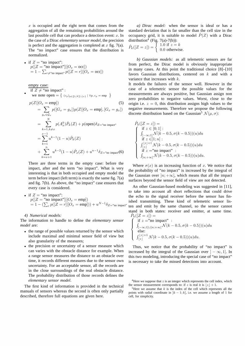
2) Dirac example:suppose that the Diracelementary sen-sor modelis the choosen model but the sensor uncertainty isa Gaussian. Despite the fact that the convolution of a Diracby a Gaussian is a Gaussian, the convolution of the Diracelementary sensor modelby a Gaussian gives an occupancyfunction with the first occupied cell6 several cells behind theobstacle cell (fig. 3).
0
0.1
0.2
0.3
0.4
0.5
0.6
0.7
0.8
0.9
1
40 50 60 70 80 90 100 110 120 130 140 150 160 170 180
Fig. 3. A 1D environement with only one obstacle in cell120, theelementarysensor modelis a Dirac one (in blue for a precise measurement). In black, themeasurement noise is a Gaussian with a std of 5 cells. In red, the occupancyfunction that results of the observation of10000 range measurements withthe noise (normalized).
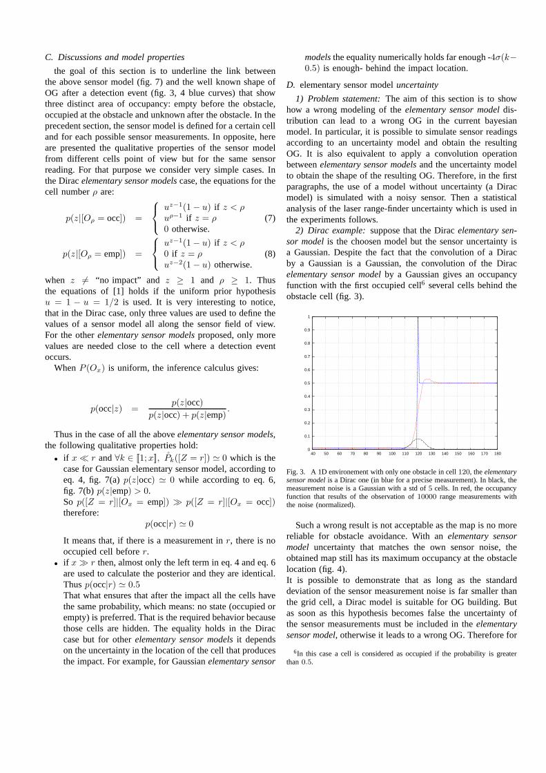
Such a wrong result is not acceptable as the map is no morereliable for obstacle avoidance. With anelementary sensormodel uncertainty that matches the own sensor noise, theobtained map still has its maximum occupancy at the obstaclelocation (fig. 4).It is possible to demonstrate that as long as the standarddeviation of the sensor measurement noise is far smaller thanthe grid cell, a Dirac model is suitable for OG building. Butas soon as this hypothesis becomes false the uncertainty ofthe sensor measurements must be included in theelementarysensor model, otherwise it leads to a wrong OG. Therefore for
6In this case a cell is considered as occupied if the probability is greaterthan0.5.
an uncertain range-finder such as stereo camera, uncertaintymust be included. But for a precise range-finder such as a laserrange-finder and large enough cells, Dirac model is suitable.Next section gives the estimated values that characterizestheuncertainty of a typical laser range-finder which allows todefine the OG and sensor model parameters.
0
0.1
0.2
0.3
0.4
0.5
0.6
0.7
0.8
0.9
1
40 50 60 70 80 90 100 110 120 130 140 150 160 170 180
Fig. 4. A 1D environement with only one obstacle in cell120, theelementarysensor modelis a Gaussian one, with a std of cells (in blue for a precisemeasurement ). In black, the measurement noise is a Gaussianwith a std of 5cells. In red, the occupancy function that results of the observation of10000range measurements with the noise (normalized).
0
0.01
0.02
0.03
0.04
0.05
0 5 10 15 20 25 30 35 40 45
Fig. 5. Estimation of the standard deviation in meter in ordinate in our dataset plotted against the mean in meter in abscissa.
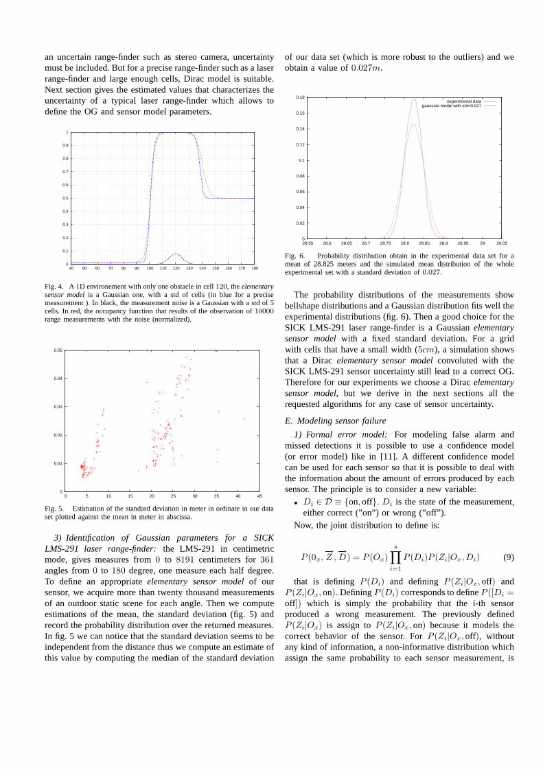
3) Identification of Gaussian parameters for a SICKLMS-291 laser range-finder:the LMS-291 in centimetricmode, gives measures from0 to 8191 centimeters for361angles from0 to 180 degree, one measure each half degree.To define an appropriateelementary sensor modelof oursensor, we acquire more than twenty thousand measurementsof an outdoor static scene for each angle. Then we computeestimations of the mean, the standard deviation (fig. 5) andrecord the probability distribution over the returned measures.In fig. 5 we can notice that the standard deviation seems to beindependent from the distance thus we compute an estimate ofthis value by computing the median of the standard deviation
of our data set (which is more robust to the outliers) and weobtain a value of0.027m.
0
0.02
0.04
0.06
0.08
0.1
0.12
0.14
0.16
0.18
28.55 28.6 28.65 28.7 28.75 28.8 28.85 28.9 28.95 29 29.05
experimental datagaussian model with std=0.027
Fig. 6. Probability distribution obtain in the experimental data set for amean of 28.825 meters and the simulated mean distribution ofthe wholeexperimental set with a standard deviation of0.027.
The probability distributions of the measurements showbellshape distributions and a Gaussian distribution fits well theexperimental distributions (fig. 6). Then a good choice for theSICK LMS-291 laser range-finder is a Gaussianelementarysensor modelwith a fixed standard deviation. For a gridwith cells that have a small width (5cm), a simulation showsthat a Diracelementary sensor modelconvoluted with theSICK LMS-291 sensor uncertainty still lead to a correct OG.Therefore for our experiments we choose a Diracelementarysensor model, but we derive in the next sections all therequested algorithms for any case of sensor uncertainty.
E. Modeling sensor failure
1) Formal error model: For modeling false alarm andmissed detections it is possible to use a confidence model(or error model) like in [11]. A different confidence modelcan be used for each sensor so that it is possible to deal withthe information about the amount of errors produced by eachsensor. The principle is to consider a new variable:
• Di ∈ D ≡ on, off. Di is the state of the measurement,either correct (”on”) or wrong (”off”).
Now, the joint distribution to define is:
P (0x,−→Z ,−→D) = P (Ox)
s∏
i=1
P (Di)P (Zi|Ox, Di) (9)
that is definingP (Di) and definingP (Zi|Ox, off) andP (Zi|Ox, on). DefiningP (Di) corresponds to defineP ([Di =off]) which is simply the probability that the i-th sensorproduced a wrong measurement. The previously definedP (Zi|Ox) is assign toP (Zi|Ox, on) because it models thecorrect behavior of the sensor. ForP (Zi|Ox, off), withoutany kind of information, a non-informative distribution whichassign the same probability to each sensor measurement, is
chosen for the two possible states,ox, of the cell.If there is no information about the current behavior of thesensor, the used distribution is just the marginalization overall the possible state of each measurement:
P (Ox,−→Z ) = P (Ox)
s∏
i=1
∑
D
P (Di)P (Zi|Ox, Di) (10)
Finally it is equivalent, to replace each sensor modelP (Zi|Ox) by the distribution:
p(on)P (Zi|Ox) + p(off)U(Zi) (11)
whereU(Zi) is a uniform distribution overZi.This kind of transformation of the sensor model adds a certaininertia related to the probability of wrong measurement. Itmeans that a good sensor measurement must be receivedseveral times to be considered by the system as relevant asa sensor measurement without error model. The more wrongmeasures are likely to occur, the more inertia the system needsto filter. This inertia is the price for the robustness added bythe fault modeling.An other very important feature added by the error model isthat it implies that all the probabilities are non zero. Thusineq. (2), p(ox,y) is never zero neither for occ, nor for emp.If not, the cell occupancy would remain always the samewhatever a sensor measurement is received. The consequencewould be an occupancy building very sensitive to sensorfailure. And it is also possible to use logarithm representationfor probabilities which increases the numerical stabilityand isrequired for the implementation of the fusion process.
0
0.05
0.1
0.15
0.2
0.25
0 5 10 15 20 25 30
(a) 0
0.05
0.1
0.15
0.2
0.25
0 5 10 15 20 25 30
(b)
0
0.02
0.04
0.06
0.08
0.1
0 5 10 15 20 25 30
(c) 0
0.02
0.04
0.06
0.08
0.1
0 5 10 15 20 25 30
(d)
Fig. 7. Probability distributions over possible sensor range measurementsknowing that the14th cell is occupied (a),(c) (resp. empty (b),(d) ). Here thesensor can return30 values of distances, the “no impact” value is not plotted,the a priori over the occupancy of cells ( the prior )u is set to0.1. (a),(b)Dirac elementary sensor models; (c),(d) Gaussianelementary sensor models.
F. Discussion and properties of the complete model
the goal of this section is to provide a numerical descriptionof the probability function in order to justify implementation
simplifications. here are presented the qualitative propertiesof the complete sensor model with failure modeling. For thatpurpose we consider the simple case of the Dirac model as inthe section II-C.
p(z|[Oρ = occ]) =
p(on)uz−1(1− u) + p(off)U(Zi) if z < ρp(on)uρ−1 + p(off)U(Zi) if z = ρp(off)U(Zi) otherwise.
(12)
p(z|[Oρ = emp]) =
p(on)uz−1(1− u) + p(off)U(Zi) if z < ρp(off)U(Zi) if z = ρp(on)uz−2(1− u) + p(off)U(Zi) otherwise.
(13)
whenz 6= “no impact”.Here is given an original theorem that states boundaries for
the occupancy of a cell when the measured distance varies.This theorem (see demonstration in appendix VIII) allows tomake approximation such that considering constants instead ofvarying function for occupancy updates in the cases of highu.
Let:
γb =1
1 + (1 + ku)l(14)
γi =k + 1
1 + k + l(15)
where:
u = 1− u (16)
k =p(on)
U(Zi)(1− p(on))(17)
l =p(emp)p(occ)
(18)
Theorem:for a cell with indexρ and a measurement atindex z and a Diracelementary sensor model,
• if ρ < z
p(occ) ∈ [γb; γb +lku
1 + (1 + ku)l(1− (1− u)z−2)],
• if ρ = z p(occ) ∈ [γi; γi +lk
1+k+l(1− (1− u)z−1)].
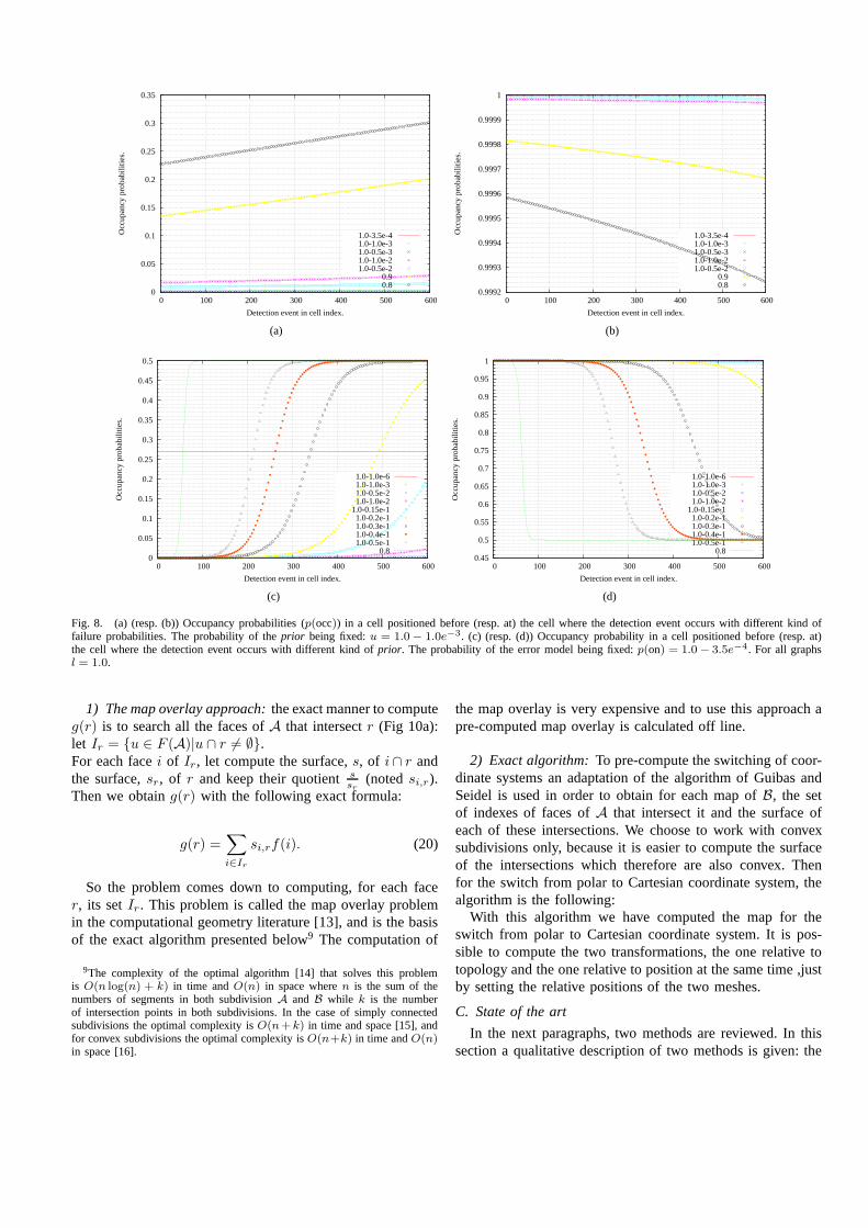
When the failure rate is fixed,i.e. for values ofu close tozero,p(occ) varies very slowly withz. In this case, the prioris very high,i.e. thea priori is that a cell is almost empty andthe occupancy of a cell tends to become independent of thedistance of the detection event (fig. 8(c)). For example, withu = 10−6, p(on) = 1.0−3.5 10−4, andl = 1 the variation allalong the600 cells of the field of view is less than1.1 10−3.The same conclusions hold for the occupancy of the cell wherethe detection event occurs (fig. 8(d)). It justifies some partof the very simple implementation of OGs like in [12], thatdecreases the occupancy of all the area before the detectedobstacle by a constant and increases the occupancy area at the
detected obstacle by a constant7. And it is a property that canspeed up the OG building if choosing such hypothesis aboutoccupancy prior. In particular, storing the whole conditionalprobability distribution over the sensor measurements foreachcell position can be avoided. It saves the memory of twomatrices ofN × (N + 1) values, one for each occupancystate occ and emp but more important: it saves all the memoryaccess to these values which is the major time consuming taskin hardware implementations (see section V).
When theprior is fixed, the change of confidence in theerror model produces a global translation of the occupancyprobability (Fig. 8(a) and 8(b)). The more failure are likely tooccur, the smaller is the change in the occupancy (occupancyis close to0.5) for each measurement.
G. Extension to 2D occupancy grids
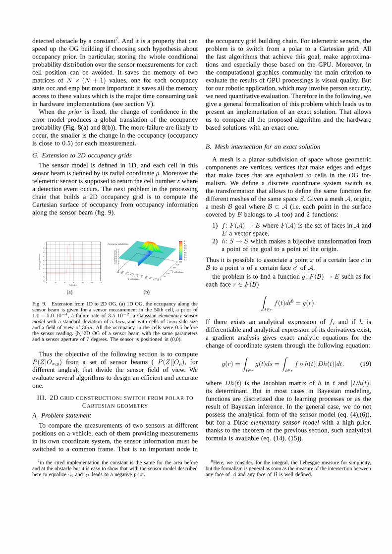
The sensor model is defined in 1D, and each cell in thissensor beam is defined by its radial coordinateρ. Moreover thetelemetric sensor is supposed to return the cell numberz wherea detection event occurs. The next problem in the processingchain that builds a 2D occupancy grid is to compute theCartesian surface of occupancy from occupancy informationalong the sensor beam (fig. 9).
0.1
0.2
0.3
0.4
0.5
0.6
0.7
0.8
0.9
1
0 20 40 60 80 100 120
Occ
upan
cy p
roba
bilit
ies.
Cell indices.
(a)
0.3 0.4 0.5 0.6 0.7 0.8 0.9 1 1.1
-25 -20 -15 -10 -5 0 5 10 15 20 25X cell indices. 0 50
100 150
200 250
300
Y cell indices.
0.2 0.3 0.4 0.5 0.6 0.7 0.8 0.9
1
Occupancy probabilities.
(b)
Fig. 9. Extension from 1D to 2D OG. (a) 1D OG, the occupancy along thesensor beam is given for a sensor measurement in the 50th cell, a prior of1.0 − 5.0 10−4, a failure rate of3.5 10−2, a Gaussianelementary sensormodelwith a standard deviation of5.4cm, and with cells of5cm side sizeand a field of view of30m. All the occupancy in the cells were0.5 beforethe sensor reading. (b) 2D OG of a sensor beam with the same parametersand a sensor aperture of7 degrees. The sensor is positioned in (0,0).
Thus the objective of the following section is to computeP (Z|Ox,y) from a set of sensor beams (P (Z|[Oρ), fordifferent angles), that divide the sensor field of view. Weevaluate several algorithms to design an efficient and accurateone.
III. 2D GRID CONSTRUCTION: SWITCH FROM POLAR TO
CARTESIAN GEOMETRY
A. Problem statement
To compare the measurements of two sensors at differentpositions on a vehicle, each of them providing measurementsin its own coordinate system, the sensor information must beswitched to a common frame. That is an important node in
7in the cited implementation the constant is the same for the area beforeand at the obstacle but it is easy to show that with the sensor model describedhere to equalizeγi andγb leads to a negative prior.
the occupancy grid building chain. For telemetric sensors,theproblem is to switch from a polar to a Cartesian grid. Allthe fast algorithms that achieve this goal, make approxima-tions and especially those based on the GPU. Moreover, inthe computational graphics community the main criterion toevaluate the results of GPU processings is visual quality. Butfor our robotic application, which may involve person security,we need quantitative evaluation. Therefore in the following, wegive a general formalization of this problem which leads us topresent an implementation of an exact solution. That allowsus to compare all the proposed algorithm and the hardwarebased solutions with an exact one.
B. Mesh intersection for an exact solution
A mesh is a planar subdivision of space whose geometriccomponents are vertices, vertices that make edges and edgesthat make faces that are equivalent to cells in the OG for-malism. We define a discrete coordinate system switch asthe transformation that allows to define the same function fordifferent meshes of the same spaceS. Given a meshA, origin,a meshB goal whereB ⊂ A (i.e. each point in the surfacecovered byB belongs toA too) and 2 functions:
1) f : F (A)→ E whereF (A) is the set of faces inA andE a vector space,
2) h: S → S which makes a bijective transformation froma point of the goal to a point of the origin.
Thus it is possible to associate a pointx of a certain facec inB to a pointu of a certain facec′ of A.
the problem is to find a functiong: F (B)→ E such as foreach facer ∈ F (B)
∫
t∈r
f(t)dt8 = g(r).
If there exists an analytical expression off , and if h isdifferentiable and analytical expression of its derivatives exist,a gradient analysis gives exact analytic equations for thechange of coordinate system through the following equation:
g(r) =
∫
t∈r
g(t)ds =
∫
t∈r
f h(t)|Dh(t)|dt. (19)
where Dh(t) is the Jacobian matrix ofh in t and |Dh(t)|its determinant. But in most cases in Bayesian modeling,functions are discretized due to learning processes or as theresult of Bayesian inference. In the general case, we do notpossess the analytical form of the sensor model (eq. (4),(6)),but for a Diracelementary sensor modelwith a high prior,thanks to the theorem of the previous section, such analyticalformula is available (eq. (14), (15)).
8Here, we consider, for the integral, the Lebesgue measure for simplicity,but the formalism is general as soon as the measure of the intersection betweenany face ofA and any face ofB is well defined.
0
0.05
0.1
0.15
0.2
0.25
0.3
0.35
0 100 200 300 400 500 600
Occ
upan
cy p
roba
bilit
ies.
Detection event in cell index.
1.0-3.5e-41.0-1.0e-31.0-0.5e-31.0-1.0e-21.0-0.5e-2
0.90.8
(a)
0.9992
0.9993
0.9994
0.9995
0.9996
0.9997
0.9998
0.9999
1
0 100 200 300 400 500 600
Occ
upan
cy p
roba
bilit
ies.
Detection event in cell index.
1.0-3.5e-41.0-1.0e-31.0-0.5e-31.0-1.0e-21.0-0.5e-2
0.90.8
(b)
0
0.05
0.1
0.15
0.2
0.25
0.3
0.35
0.4
0.45
0.5
0 100 200 300 400 500 600
Occ
upan
cy p
roba
bilit
ies.
Detection event in cell index.
1.0-1.0e-61.0-1.0e-31.0-0.5e-21.0-1.0e-2
1.0-0.15e-11.0-0.2e-11.0-0.3e-11.0-0.4e-11.0-0.5e-1
0.8
(c)
0.45
0.5
0.55
0.6
0.65
0.7
0.75
0.8
0.85
0.9
0.95
1
0 100 200 300 400 500 600
Occ
upan
cy p
roba
bilit
ies.
Detection event in cell index.
1.0-1.0e-61.0-1.0e-31.0-0.5e-21.0-1.0e-2
1.0-0.15e-11.0-0.2e-11.0-0.3e-11.0-0.4e-11.0-0.5e-1
0.8
(d)
Fig. 8. (a) (resp. (b)) Occupancy probabilities (p(occ)) in a cell positioned before (resp. at) the cell where the detection event occurs with different kind offailure probabilities. The probability of theprior being fixed:u = 1.0 − 1.0e−3. (c) (resp. (d)) Occupancy probability in a cell positionedbefore (resp. at)the cell where the detection event occurs with different kind of prior. The probability of the error model being fixed:p(on) = 1.0 − 3.5e−4. For all graphsl = 1.0.
1) The map overlay approach:the exact manner to computeg(r) is to search all the faces ofA that intersectr (Fig 10a):let Ir = u ∈ F (A)|u ∩ r 6= ∅.For each facei of Ir, let compute the surface,s, of i∩ r andthe surface,sr, of r and keep their quotients
sr(notedsi,r).
Then we obtaing(r) with the following exact formula:
g(r) =∑
i∈Ir
si,rf(i). (20)
So the problem comes down to computing, for each facer, its setIr. This problem is called the map overlay problemin the computational geometry literature [13], and is the basisof the exact algorithm presented below9 The computation of
9The complexity of the optimal algorithm [14] that solves this problemis O(n log(n) + k) in time andO(n) in space wheren is the sum of thenumbers of segments in both subdivisionA and B while k is the numberof intersection points in both subdivisions. In the case of simply connectedsubdivisions the optimal complexity isO(n+ k) in time and space [15], andfor convex subdivisions the optimal complexity isO(n+k) in time andO(n)in space [16].
the map overlay is very expensive and to use this approach apre-computed map overlay is calculated off line.
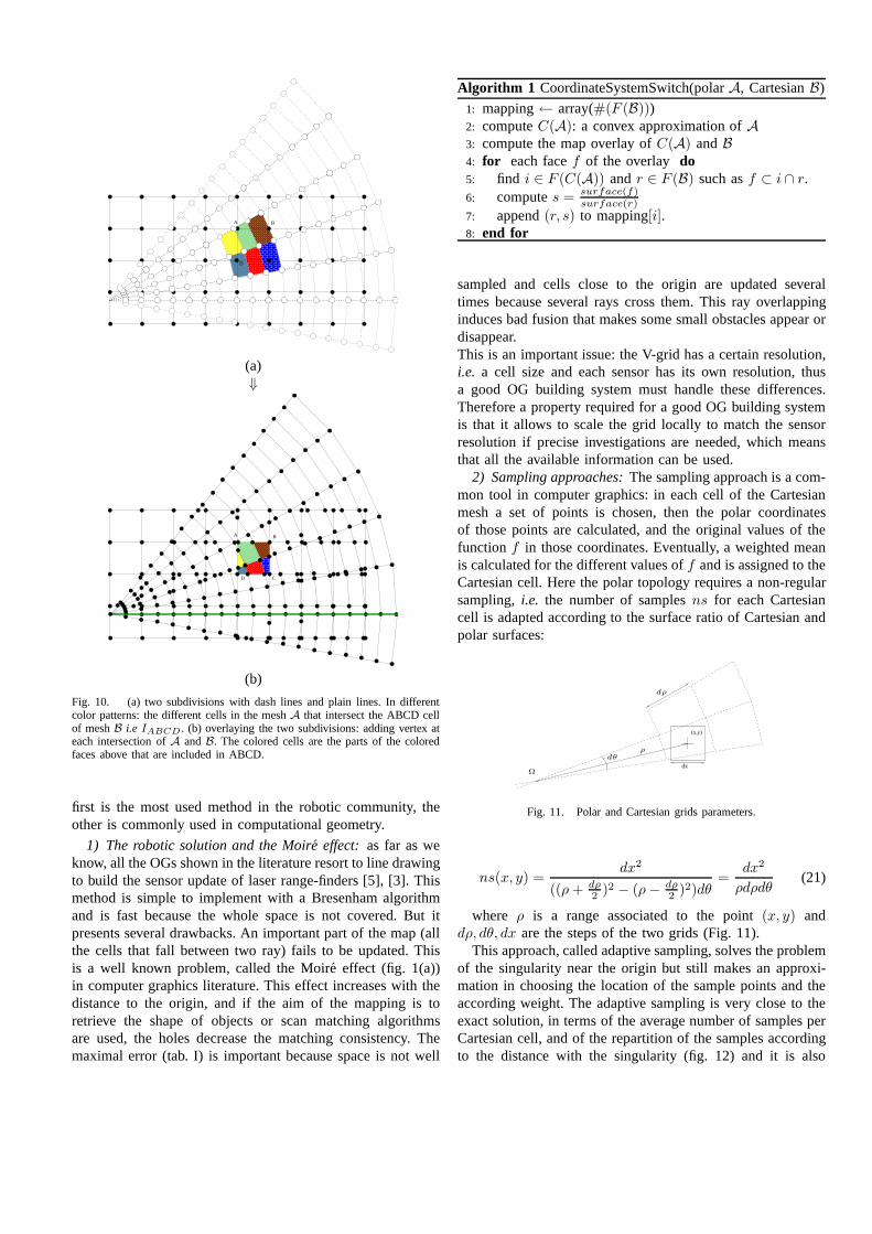
2) Exact algorithm:To pre-compute the switching of coor-dinate systems an adaptation of the algorithm of Guibas andSeidel is used in order to obtain for each map ofB, the setof indexes of faces ofA that intersect it and the surface ofeach of these intersections. We choose to work with convexsubdivisions only, because it is easier to compute the surfaceof the intersections which therefore are also convex. Thenfor the switch from polar to Cartesian coordinate system, thealgorithm is the following:
With this algorithm we have computed the map for theswitch from polar to Cartesian coordinate system. It is pos-sible to compute the two transformations, the one relative totopology and the one relative to position at the same time ,justby setting the relative positions of the two meshes.
C. State of the art
In the next paragraphs, two methods are reviewed. In thissection a qualitative description of two methods is given: the
A B
D C
(a)⇓
A B
CD
(b)
Fig. 10. (a) two subdivisions with dash lines and plain lines. In differentcolor patterns: the different cells in the meshA that intersect the ABCD cellof meshB i.e IABCD . (b) overlaying the two subdivisions: adding vertex ateach intersection ofA andB. The colored cells are the parts of the coloredfaces above that are included in ABCD.
first is the most used method in the robotic community, theother is commonly used in computational geometry.
1) The robotic solution and the Moire effect: as far as weknow, all the OGs shown in the literature resort to line drawingto build the sensor update of laser range-finders [5], [3]. Thismethod is simple to implement with a Bresenham algorithmand is fast because the whole space is not covered. But itpresents several drawbacks. An important part of the map (allthe cells that fall between two ray) fails to be updated. Thisis a well known problem, called the Moire effect (fig. 1(a))in computer graphics literature. This effect increases with thedistance to the origin, and if the aim of the mapping is toretrieve the shape of objects or scan matching algorithmsare used, the holes decrease the matching consistency. Themaximal error (tab. I) is important because space is not well
Algorithm 1 CoordinateSystemSwitch(polarA, CartesianB)
1: mapping← array(#(F (B)))2: computeC(A): a convex approximation ofA3: compute the map overlay ofC(A) andB4: for each facef of the overlay do5: find i ∈ F (C(A)) andr ∈ F (B) such asf ⊂ i ∩ r.6: computes = surface(f)
surface(r)
7: append(r, s) to mapping[i].8: end for
sampled and cells close to the origin are updated severaltimes because several rays cross them. This ray overlappinginduces bad fusion that makes some small obstacles appear ordisappear.This is an important issue: the V-grid has a certain resolution,i.e. a cell size and each sensor has its own resolution, thusa good OG building system must handle these differences.Therefore a property required for a good OG building systemis that it allows to scale the grid locally to match the sensorresolution if precise investigations are needed, which meansthat all the available information can be used.
2) Sampling approaches:The sampling approach is a com-mon tool in computer graphics: in each cell of the Cartesianmesh a set of points is chosen, then the polar coordinatesof those points are calculated, and the original values of thefunction f in those coordinates. Eventually, a weighted meanis calculated for the different values off and is assigned to theCartesian cell. Here the polar topology requires a non-regularsampling,i.e. the number of samplesns for each Cartesiancell is adapted according to the surface ratio of Cartesian andpolar surfaces:
(x,y)
dx
dρ
ρdθ
Ω
Fig. 11. Polar and Cartesian grids parameters.
ns(x, y) =dx2
((ρ + dρ2 )2 − (ρ− dρ
2 )2)dθ=
dx2
ρdρdθ(21)
where ρ is a range associated to the point(x, y) anddρ, dθ, dx are the steps of the two grids (Fig. 11).
This approach, called adaptive sampling, solves the problemof the singularity near the origin but still makes an approxi-mation in choosing the location of the sample points and theaccording weight. The adaptive sampling is very close to theexact solution, in terms of the average number of samples perCartesian cell, and of the repartition of the samples accordingto the distance with the singularity (fig. 12) and it is also
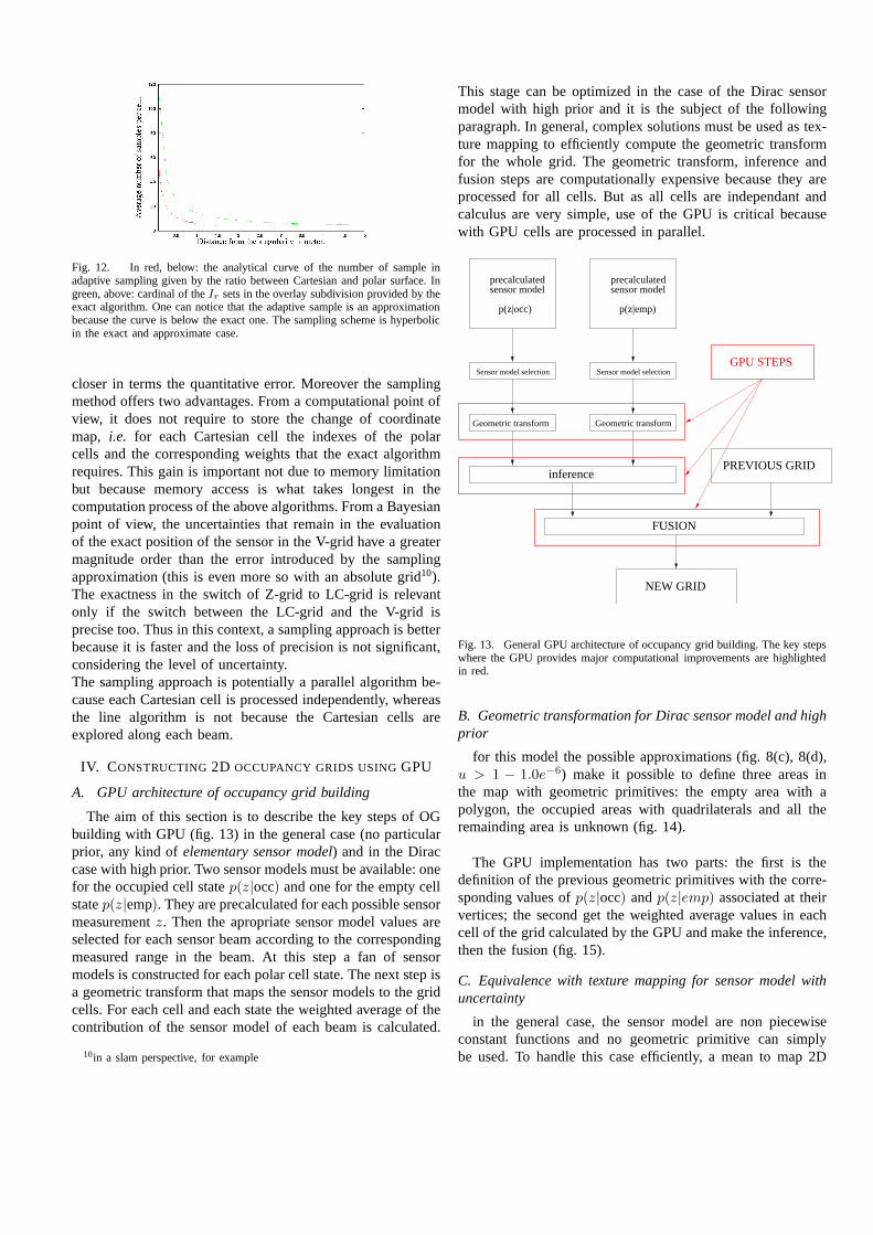
Fig. 12. In red, below: the analytical curve of the number of sample inadaptive sampling given by the ratio between Cartesian and polar surface. Ingreen, above: cardinal of theIr sets in the overlay subdivision provided by theexact algorithm. One can notice that the adaptive sample is an approximationbecause the curve is below the exact one. The sampling schemeis hyperbolicin the exact and approximate case.
closer in terms the quantitative error. Moreover the samplingmethod offers two advantages. From a computational point ofview, it does not require to store the change of coordinatemap, i.e. for each Cartesian cell the indexes of the polarcells and the corresponding weights that the exact algorithmrequires. This gain is important not due to memory limitationbut because memory access is what takes longest in thecomputation process of the above algorithms. From a Bayesianpoint of view, the uncertainties that remain in the evaluationof the exact position of the sensor in the V-grid have a greatermagnitude order than the error introduced by the samplingapproximation (this is even more so with an absolute grid10).The exactness in the switch of Z-grid to LC-grid is relevantonly if the switch between the LC-grid and the V-grid isprecise too. Thus in this context, a sampling approach is betterbecause it is faster and the loss of precision is not significant,considering the level of uncertainty.The sampling approach is potentially a parallel algorithm be-cause each Cartesian cell is processed independently, whereasthe line algorithm is not because the Cartesian cells areexplored along each beam.
IV. CONSTRUCTING2D OCCUPANCY GRIDS USINGGPU
A. GPU architecture of occupancy grid building
The aim of this section is to describe the key steps of OGbuilding with GPU (fig. 13) in the general case (no particularprior, any kind ofelementary sensor model) and in the Diraccase with high prior. Two sensor models must be available: onefor the occupied cell statep(z|occ) and one for the empty cellstatep(z|emp). They are precalculated for each possible sensormeasurementz. Then the apropriate sensor model values areselected for each sensor beam according to the correspondingmeasured range in the beam. At this step a fan of sensormodels is constructed for each polar cell state. The next step isa geometric transform that maps the sensor models to the gridcells. For each cell and each state the weighted average of thecontribution of the sensor model of each beam is calculated.
10in a slam perspective, for example
This stage can be optimized in the case of the Dirac sensormodel with high prior and it is the subject of the followingparagraph. In general, complex solutions must be used as tex-ture mapping to efficiently compute the geometric transformfor the whole grid. The geometric transform, inference andfusion steps are computationally expensive because they areprocessed for all cells. But as all cells are independant andcalculus are very simple, use of the GPU is critical becausewith GPU cells are processed in parallel.
FUSION
NEW GRID
inferencePREVIOUS GRID
GPU STEPS
p(z|occ)
precalculatedsensor model
p(z|emp)
precalculatedsensor model
Geometric transform Geometric transform
Sensor model selectionSensor model selection
Fig. 13. General GPU architecture of occupancy grid building. The key stepswhere the GPU provides major computational improvements are highlightedin red.
B. Geometric transformation for Dirac sensor model and highprior
for this model the possible approximations (fig. 8(c), 8(d),u > 1 − 1.0e−6) make it possible to define three areas inthe map with geometric primitives: the empty area with apolygon, the occupied areas with quadrilaterals and all theremainding area is unknown (fig. 14).
The GPU implementation has two parts: the first is thedefinition of the previous geometric primitives with the corre-sponding values ofp(z|occ) andp(z|emp) associated at theirvertices; the second get the weighted average values in eachcell of the grid calculated by the GPU and make the inference,then the fusion (fig. 15).
C. Equivalence with texture mapping for sensor model withuncertainty
in the general case, the sensor model are non piecewiseconstant functions and no geometric primitive can simplybe used. To handle this case efficiently, a mean to map 2D
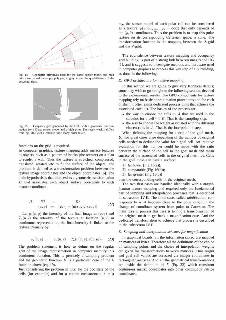
Fig. 14. Geometric primitives used for the Dirac sensor model and highprior case: in red the empty polygon, in grey stripes the quadrilaterals of theoccupied areas.
Fig. 15. Occupancy grid generated by the GPU with a geometrictransfor-mation for a Dirac sensor model and a high prior. The result weakly differsfrom fig. 1(b) with a calculus time many order faster.
functions on the grid is required.In computer graphics, texture mapping adds surface featuresto objects, such as a pattern of bricks (the texture) on a planto render a wall. Thus the texture is stretched, compressed,translated, rotated, etc to fit the surface of the object. Theproblem is defined as a transformation problem between thetexture image coordinates and the object coordinates [6]. Themain hypothesis is that there exists a geometric transformationH that associates each object surface coordinate to eachtexture coordinate:
H : R2 → R2
(x, y) 7→ (u, v) = (u(x, y), v(x, y))(22)
Let ga(x, y) the intensity of the final image at(x, y) andTa(u, v) the intensity of the texture at location(u, v) incontinuous representation, the final intensity is linked tothetexture intensity by:
ga(x, y) = Ta(u, v) = Ta(u(x, y), v(x, y)). (23)
The problem statement is how to define on the regulargrid of the image representation in computer memory thiscontinuous function. This is precisely a sampling problemand the geometric functionH is a particular case of thehfunction above (eq. 19).Just considering the problem in OG: for the occ state of thecells (for example) and for a certain measurementz in a
ray, the sensor model of each polar cell can be consideredas a texture:p(z|[O(u,v)=(ρ,θ) = occ]) that only depends ofthe (ρ, θ) coordinates. Thus the problem is to map this polartexture on its corresponding Cartesian space: a cone. Thetransformation function is the mapping between the Z-gridand the V-grid.
The equivalence between texture mapping and occupancygrid building, is part of a strong link between images and OG[1], and it suggests to investigate methods and hardware usedin computer graphics to process this key step of OG building,as done in the following.
D. GPU architecture for texture mapping
In this section we are going to give very technical details;some may wish to go straight to the following section, devotedto the experimental results. The GPU components for texturemapping rely on basic approximation procedures and for eachof them it often exists dedicated process units that achievetheassociated calculus. The basics of the process are
• the way to choose the cells inA that are used in thecalculus for a cellr ∈ B. That is the sampling step.
• the way to choose the weight associated with the differentchosen cells inA. That is the interpolation step.
When defining the mapping for a cell of the goal mesh,B, two great cases arise depending of the number of originalcells needed to deduce the value for a goal cell. An intuitiveevaluation for this number could be made with the ratiobetween the surface of the cell in the goal mesh and meansurface of the associated cells in the original mesh,A. Cellsin the goal mesh can have a surface:
1) far lower (Fig 16(a));2) comparable (Fig 16(b));3) far greater (Fig 16(c))
than the corresponding cells in the original mesh.The two first cases are handled identically with amagni-
fication texture mapping and required only the fundamentalpart of sampling and interpolation processes that is describedin subsection IV-E. The third case, calledminification, cor-responds to what happens close to the polar origin in thechange of coordinate system from polar to Cartesian. Themain idea to process this case is to find a transformation ofthe original mesh to get back a magnification case. And thededicated transformation to achieve that process is describedin the subsection IV-F.
E. Sampling and interpolation schemes for magnification
In graphical boards, all the information stored are mappedon matrices of bytes. Therefore all the definitions of the choiceof sampling points and the choice of interpolation weightsare given for transformations between matrices. Thus originand goal cell values are accessed via integer coordinates inrectangular matrices. And all the geometrical transformationsare inside the definition ofF (Eq. 22) which transformcontinuous matrix coordinates into other continuous Patricecoordinates.
(a) (b) (c)
Fig. 16. (a) and (b) cases of magnification: the goal cell overlap with few cells in the original mesh. (c) case of minification: the goal cell overlap manycells in the original mesh.
0 1 2
0.4 0.6
[0.0;3.0]
A
B
c0(0.5) c1(0.5)
sample:u(0.9)
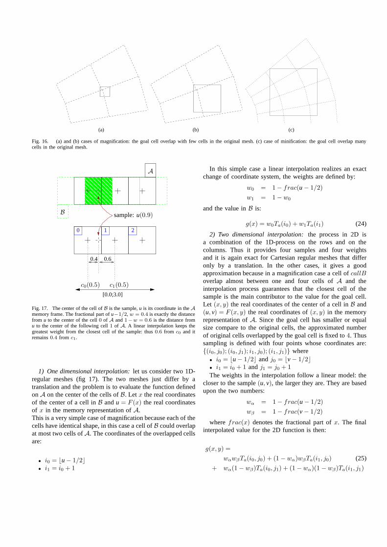
Fig. 17. The center of the cell ofB is the sample,u is its coordinate in theAmemory frame. The fractional part ofu−1/2, w = 0.4 is exactly the distancefrom u to the center of the cell0 of A and1−w = 0.6 is the distance fromu to the center of the following cell1 of A. A linear interpolation keeps thegreatest weight from the closest cell of the sample: thus0.6 from c0 and itremains0.4 from c1.
1) One dimensional interpolation:let us consider two 1D-regular meshes (fig 17). The two meshes just differ by atranslation and the problem is to evaluate the function definedonA on the center of the cells ofB. Let x the real coordinatesof the center of a cell inB andu = F (x) the real coordinatesof x in the memory representation ofA.This is a very simple case of magnification because each of thecells have identical shape, in this case a cell ofB could overlapat most two cells ofA. The coordinates of the overlapped cellsare:
• i0 = ⌊u− 1/2⌋• i1 = i0 + 1
In this simple case a linear interpolation realizes an exactchange of coordinate system, the weights are defined by:
w0 = 1− frac(u− 1/2)
w1 = 1− w0
and the value inB is:
g(x) = w0Ta(i0) + w1Ta(i1) (24)
2) Two dimensional interpolation:the process in 2D isa combination of the 1D-process on the rows and on thecolumns. Thus it provides four samples and four weightsand it is again exact for Cartesian regular meshes that differonly by a translation. In the other cases, it gives a goodapproximation because in a magnification case a cell ofcallBoverlap almost between one and four cells ofA and theinterpolation process guarantees that the closest cell of thesample is the main contributor to the value for the goal cell.Let (x, y) the real coordinates of the center of a cell inB and(u, v) = F (x, y) the real coordinates of(x, y) in the memoryrepresentation ofA. Since the goal cell has smaller or equalsize compare to the original cells, the approximated numberof original cells overlapped by the goal cell is fixed to4. Thussampling is defined with four points whose coordinates are:(i0, j0); (i0, j1); i1, j0); (i1, j1) where
• i0 = ⌊u− 1/2⌋ andj0 = ⌊v− 1/2⌋• i1 = i0 + 1 andj1 = j0 + 1
The weights in the interpolation follow a linear model: thecloser to the sample(u, v), the larger they are. They are basedupon the two numbers:
wα = 1− frac(u− 1/2)
wβ = 1− frac(v− 1/2)
wherefrac(x) denotes the fractional part ofx. The finalinterpolated value for the 2D function is then:
g(x, y) =
wαwβTa(i0, j0) + (1− wα)wβTa(i1, j0) (25)
+ wα(1 − wβ)Ta(i0, j1) + (1− wα)(1 − wβ)Ta(i1, j1)
F. Minification and mipmapping
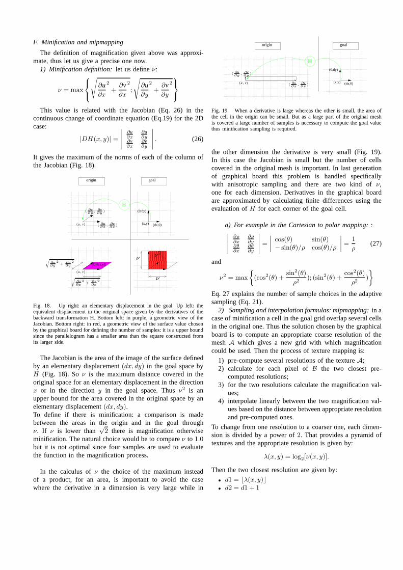
The definition of magnification given above was approxi-mate, thus let us give a precise one now.
1) Minification definition: let us defineν:
ν = max
√
∂u∂x
2
+∂v∂x
2
;
√
∂u∂y
2
+∂v∂y
2
This value is related with the Jacobian (Eq. 26) in thecontinuous change of coordinate equation (Eq.19) for the 2Dcase:
|DH(x, y)| =∣
∣
∣
∣
∣
∂u∂x
∂u∂y
∂v∂x
∂v∂y
∣
∣
∣
∣
∣
. (26)
It gives the maximum of the norms of each of the column ofthe Jacobian (Fig. 18).
origin goal
(x,y) (dx,0)
(0,dy)
H
|DH(x,y)|
(u, v)
(u, v)
( ∂u∂y
, ∂v∂y
)
( ∂u∂x
, ∂v∂x
)
r
∂u∂x
2+ ∂v
∂x2
r
∂u∂y
2+ ∂v
∂y2
ν
ν
ν2
Fig. 18. Up right: an elementary displacement in the goal. Upleft: theequivalent displacement in the original space given by the derivatives of thebackward transformation H. Bottom left: in purple, a geometric view of theJacobian. Bottom right: in red, a geometric view of the surface value chosenby the graphical board for defining the number of samples: it is a upper boundsince the parallelogram has a smaller area than the square constructed fromits larger side.
The Jacobian is the area of the image of the surface definedby an elementary displacement(dx, dy) in the goal space byH (Fig. 18). Soν is the maximum distance covered in theoriginal space for an elementary displacement in the directionx or in the directiony in the goal space. Thusν2 is anupper bound for the area covered in the original space by anelementary displacement(dx, dy).To define if there is minification: a comparison is madebetween the areas in the origin and in the goal throughν. If ν is lower than
√2 there is magnification otherwise
minification. The natural choice would be to compareν to 1.0but it is not optimal since four samples are used to evaluatethe function in the magnification process.
In the calculus ofν the choice of the maximum insteadof a product, for an area, is important to avoid the casewhere the derivative in a dimension is very large while in
origin
(x,y) (dx,0)
(0,dy)
goal
H
(u, v)
( ∂u∂y
, ∂v∂y
)
( ∂u∂x
, ∂v∂x
)
Fig. 19. When a derivative is large whereas the other is small, the area ofthe cell in the origin can be small. But as a large part of the original meshis covered a large number of samples is necessary to compute the goal valuethus minification sampling is required.
the other dimension the derivative is very small (Fig. 19).In this case the Jacobian is small but the number of cellscovered in the original mesh is important. In last generationof graphical board this problem is handled specificallywith anisotropic sampling and there are two kind ofν,one for each dimension. Derivatives in the graphical boardare approximated by calculating finite differences using theevaluation ofH for each corner of the goal cell.
a) For example in the Cartesian to polar mapping: :∣
∣
∣
∣
∣
∂ρ∂x
∂ρ∂y
∂θ∂x
∂θ∂y
∣
∣
∣
∣
∣
=
∣
∣
∣
∣
cos(θ) sin(θ)− sin(θ)/ρ cos(θ)/ρ
∣
∣
∣
∣
=1
ρ(27)
and
ν2 = max
(cos2(θ) +sin2(θ)
ρ2); (sin2(θ) +
cos2(θ)
ρ2)
Eq. 27 explains the number of sample choices in the adaptivesampling (Eq. 21).
2) Sampling and interpolation formulas: mipmapping:in acase of minification a cell in the goal grid overlap several cellsin the original one. Thus the solution chosen by the graphicalboard is to compute an appropriate coarse resolution of themeshA which gives a new grid with which magnificationcould be used. Then the process of texture mapping is:
1) pre-compute several resolutions of the textureA;2) calculate for each pixel ofB the two closest pre-
computed resolutions;3) for the two resolutions calculate the magnification val-
ues;4) interpolate linearly between the two magnification val-
ues based on the distance between appropriate resolutionand pre-computed ones.
To change from one resolution to a coarser one, each dimen-sion is divided by a power of2. That provides a pyramid oftextures and the appropriate resolution is given by:
λ(x, y) = log2[ν(x, y)].
Then the two closest resolution are given by:
• d1 = ⌊λ(x, y)⌋• d2 = d1 + 1
The magnification rules for sampling and interpolating are thenapplied to each of the selected texture, yielding two corre-sponding valuesg1(x, y) for the d1 resolution andg2(x, y)for d2 resolution. The final value for the cell(x, y) is thenfound as a 1D interpolation between the two resolutions:
g(x, y) = (1−frac(λ(x, y)))g1(x, y)+frac(λ(x, y))g2(x, y)
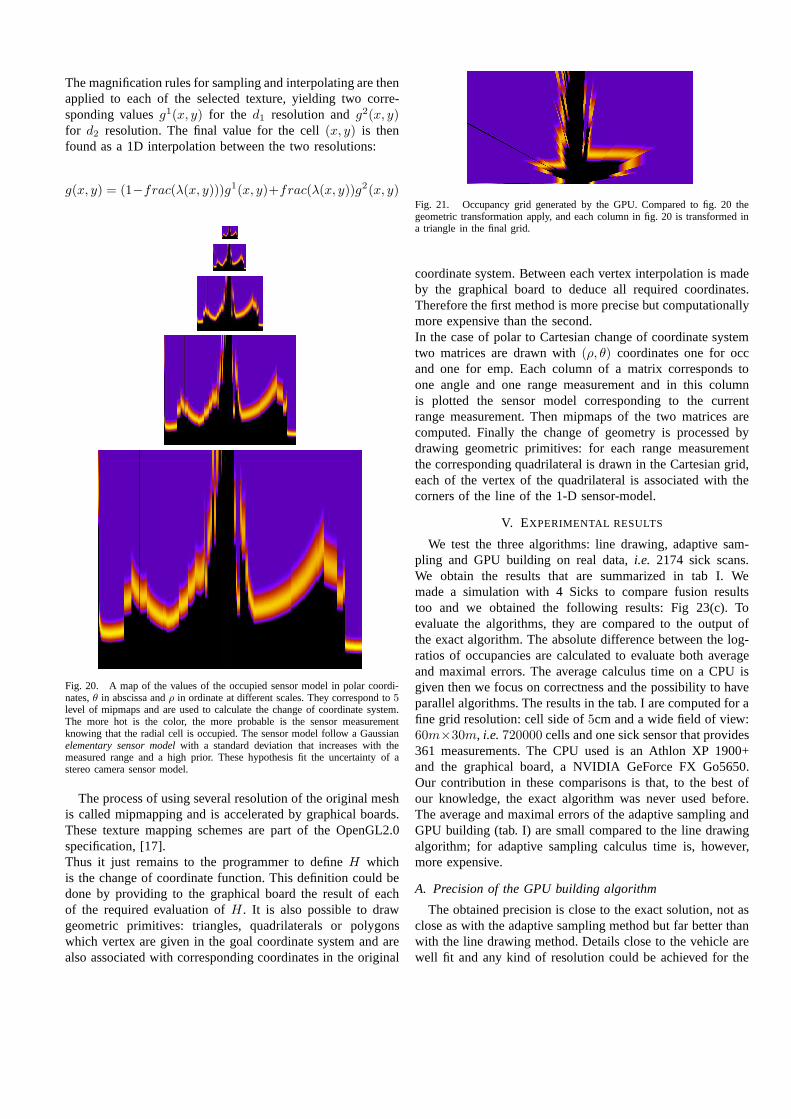
Fig. 20. A map of the values of the occupied sensor model in polar coordi-nates,θ in abscissa andρ in ordinate at different scales. They correspond to5level of mipmaps and are used to calculate the change of coordinate system.The more hot is the color, the more probable is the sensor measurementknowing that the radial cell is occupied. The sensor model follow a Gaussianelementary sensor modelwith a standard deviation that increases with themeasured range and a high prior. These hypothesis fit the uncertainty of astereo camera sensor model.
The process of using several resolution of the original meshis called mipmapping and is accelerated by graphical boards.These texture mapping schemes are part of the OpenGL2.0specification, [17].Thus it just remains to the programmer to defineH whichis the change of coordinate function. This definition could bedone by providing to the graphical board the result of eachof the required evaluation ofH . It is also possible to drawgeometric primitives: triangles, quadrilaterals or polygonswhich vertex are given in the goal coordinate system and arealso associated with corresponding coordinates in the original
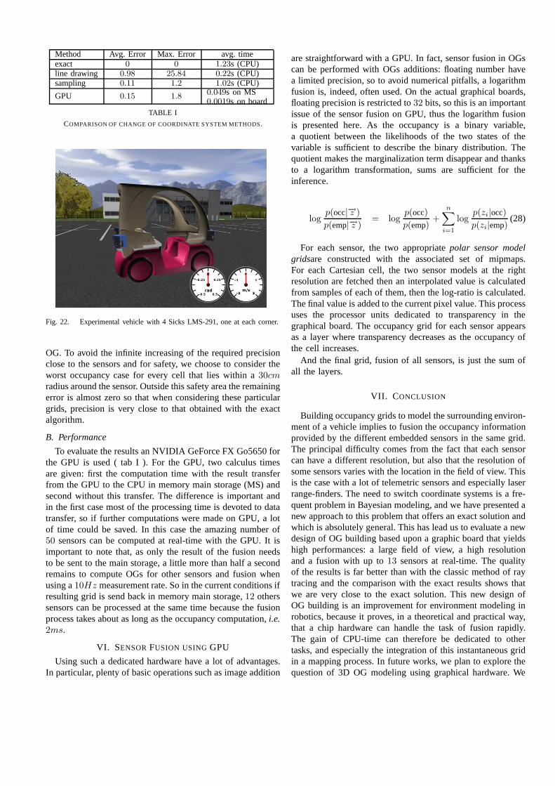
Fig. 21. Occupancy grid generated by the GPU. Compared to fig.20 thegeometric transformation apply, and each column in fig. 20 istransformed ina triangle in the final grid.
coordinate system. Between each vertex interpolation is madeby the graphical board to deduce all required coordinates.Therefore the first method is more precise but computationallymore expensive than the second.In the case of polar to Cartesian change of coordinate systemtwo matrices are drawn with(ρ, θ) coordinates one for occand one for emp. Each column of a matrix corresponds toone angle and one range measurement and in this columnis plotted the sensor model corresponding to the currentrange measurement. Then mipmaps of the two matrices arecomputed. Finally the change of geometry is processed bydrawing geometric primitives: for each range measurementthe corresponding quadrilateral is drawn in the Cartesian grid,each of the vertex of the quadrilateral is associated with thecorners of the line of the 1-D sensor-model.
V. EXPERIMENTAL RESULTS
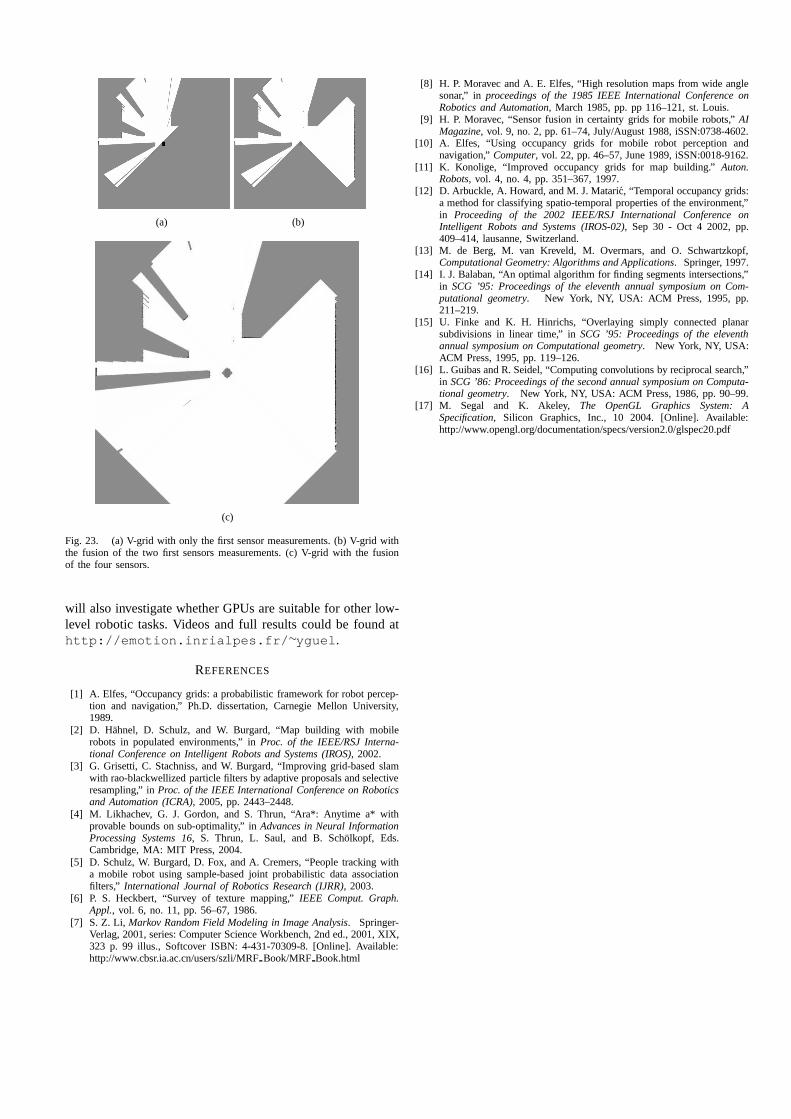
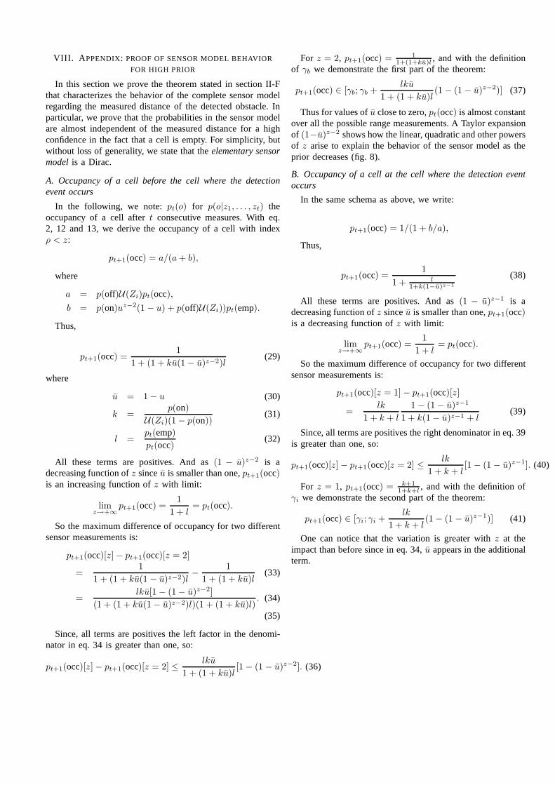
We test the three algorithms: line drawing, adaptive sam-pling and GPU building on real data,i.e. 2174 sick scans.We obtain the results that are summarized in tab I. Wemade a simulation with 4 Sicks to compare fusion resultstoo and we obtained the following results: Fig 23(c). Toevaluate the algorithms, they are compared to the output ofthe exact algorithm. The absolute difference between the log-ratios of occupancies are calculated to evaluate both averageand maximal errors. The average calculus time on a CPU isgiven then we focus on correctness and the possibility to haveparallel algorithms. The results in the tab. I are computed for afine grid resolution: cell side of5cm and a wide field of view:60m×30m, i.e.720000 cells and one sick sensor that provides361 measurements. The CPU used is an Athlon XP 1900+and the graphical board, a NVIDIA GeForce FX Go5650.Our contribution in these comparisons is that, to the best ofour knowledge, the exact algorithm was never used before.The average and maximal errors of the adaptive sampling andGPU building (tab. I) are small compared to the line drawingalgorithm; for adaptive sampling calculus time is, however,more expensive.
A. Precision of the GPU building algorithm
The obtained precision is close to the exact solution, not asclose as with the adaptive sampling method but far better thanwith the line drawing method. Details close to the vehicle arewell fit and any kind of resolution could be achieved for the
Method Avg. Error Max. Error avg. timeexact 0 0 1.23s (CPU)line drawing 0.98 25.84 0.22s (CPU)sampling 0.11 1.2 1.02s (CPU)
GPU 0.15 1.80.049s on MS0.0019s on board
TABLE I
COMPARISON OF CHANGE OF COORDINATE SYSTEM METHODS.
Fig. 22. Experimental vehicle with 4 Sicks LMS-291, one at each corner.
OG. To avoid the infinite increasing of the required precisionclose to the sensors and for safety, we choose to consider theworst occupancy case for every cell that lies within a30cmradius around the sensor. Outside this safety area the remainingerror is almost zero so that when considering these particulargrids, precision is very close to that obtained with the exactalgorithm.
B. Performance
To evaluate the results an NVIDIA GeForce FX Go5650 forthe GPU is used ( tab I ). For the GPU, two calculus timesare given: first the computation time with the result transferfrom the GPU to the CPU in memory main storage (MS) andsecond without this transfer. The difference is important andin the first case most of the processing time is devoted to datatransfer, so if further computations were made on GPU, a lotof time could be saved. In this case the amazing number of50 sensors can be computed at real-time with the GPU. It isimportant to note that, as only the result of the fusion needsto be sent to the main storage, a little more than half a secondremains to compute OGs for other sensors and fusion whenusing a10Hz measurement rate. So in the current conditions ifresulting grid is send back in memory main storage,12 otherssensors can be processed at the same time because the fusionprocess takes about as long as the occupancy computation,i.e.2ms.
VI. SENSORFUSION USINGGPU
Using such a dedicated hardware have a lot of advantages.In particular, plenty of basic operations such as image addition
are straightforward with a GPU. In fact, sensor fusion in OGscan be performed with OGs additions: floating number havea limited precision, so to avoid numerical pitfalls, a logarithmfusion is, indeed, often used. On the actual graphical boards,floating precision is restricted to32 bits, so this is an importantissue of the sensor fusion on GPU, thus the logarithm fusionis presented here. As the occupancy is a binary variable,a quotient between the likelihoods of the two states of thevariable is sufficient to describe the binary distribution.Thequotient makes the marginalization term disappear and thanksto a logarithm transformation, sums are sufficient for theinference.
logp(occ|−→z )
p(emp|−→z )= log
p(occ)
p(emp)+
n∑
i=1
logp(zi|occ)
p(zi|emp)(28)
For each sensor, the two appropriatepolar sensor modelgridsare constructed with the associated set of mipmaps.For each Cartesian cell, the two sensor models at the rightresolution are fetched then an interpolated value is calculatedfrom samples of each of them, then the log-ratio is calculated.The final value is added to the current pixel value. This processuses the processor units dedicated to transparency in thegraphical board. The occupancy grid for each sensor appearsas a layer where transparency decreases as the occupancy ofthe cell increases.
And the final grid, fusion of all sensors, is just the sum ofall the layers.
VII. C ONCLUSION
Building occupancy grids to model the surrounding environ-ment of a vehicle implies to fusion the occupancy informationprovided by the different embedded sensors in the same grid.The principal difficulty comes from the fact that each sensorcan have a different resolution, but also that the resolution ofsome sensors varies with the location in the field of view. Thisis the case with a lot of telemetric sensors and especially laserrange-finders. The need to switch coordinate systems is a fre-quent problem in Bayesian modeling, and we have presented anew approach to this problem that offers an exact solution andwhich is absolutely general. This has lead us to evaluate a newdesign of OG building based upon a graphic board that yieldshigh performances: a large field of view, a high resolutionand a fusion with up to13 sensors at real-time. The qualityof the results is far better than with the classic method of raytracing and the comparison with the exact results shows thatwe are very close to the exact solution. This new design ofOG building is an improvement for environment modeling inrobotics, because it proves, in a theoretical and practicalway,that a chip hardware can handle the task of fusion rapidly.The gain of CPU-time can therefore be dedicated to othertasks, and especially the integration of this instantaneous gridin a mapping process. In future works, we plan to explore thequestion of 3D OG modeling using graphical hardware. We
(a) (b)
(c)
Fig. 23. (a) V-grid with only the first sensor measurements. (b) V-grid withthe fusion of the two first sensors measurements. (c) V-grid with the fusionof the four sensors.
will also investigate whether GPUs are suitable for other low-level robotic tasks. Videos and full results could be found athttp://emotion.inrialpes.fr/∼yguel.
REFERENCES
[1] A. Elfes, “Occupancy grids: a probabilistic framework for robot percep-tion and navigation,” Ph.D. dissertation, Carnegie MellonUniversity,1989.
[2] D. Hahnel, D. Schulz, and W. Burgard, “Map building withmobilerobots in populated environments,” inProc. of the IEEE/RSJ Interna-tional Conference on Intelligent Robots and Systems (IROS), 2002.
[3] G. Grisetti, C. Stachniss, and W. Burgard, “Improving grid-based slamwith rao-blackwellized particle filters by adaptive proposals and selectiveresampling,” inProc. of the IEEE International Conference on Roboticsand Automation (ICRA), 2005, pp. 2443–2448.
[4] M. Likhachev, G. J. Gordon, and S. Thrun, “Ara*: Anytime a* withprovable bounds on sub-optimality,” inAdvances in Neural InformationProcessing Systems 16, S. Thrun, L. Saul, and B. Scholkopf, Eds.Cambridge, MA: MIT Press, 2004.
[5] D. Schulz, W. Burgard, D. Fox, and A. Cremers, “People tracking witha mobile robot using sample-based joint probabilistic dataassociationfilters,” International Journal of Robotics Research (IJRR), 2003.
[6] P. S. Heckbert, “Survey of texture mapping,”IEEE Comput. Graph.Appl., vol. 6, no. 11, pp. 56–67, 1986.
[7] S. Z. Li, Markov Random Field Modeling in Image Analysis. Springer-Verlag, 2001, series: Computer Science Workbench, 2nd ed.,2001, XIX,323 p. 99 illus., Softcover ISBN: 4-431-70309-8. [Online].Available:http://www.cbsr.ia.ac.cn/users/szli/MRFBook/MRF Book.html
[8] H. P. Moravec and A. E. Elfes, “High resolution maps from wide anglesonar,” in proceedings of the 1985 IEEE International Conference onRobotics and Automation, March 1985, pp. pp 116–121, st. Louis.
[9] H. P. Moravec, “Sensor fusion in certainty grids for mobile robots,”AIMagazine, vol. 9, no. 2, pp. 61–74, July/August 1988, iSSN:0738-4602.
[10] A. Elfes, “Using occupancy grids for mobile robot perception andnavigation,”Computer, vol. 22, pp. 46–57, June 1989, iSSN:0018-9162.
[11] K. Konolige, “Improved occupancy grids for map building.” Auton.Robots, vol. 4, no. 4, pp. 351–367, 1997.
[12] D. Arbuckle, A. Howard, and M. J. Mataric, “Temporal occupancy grids:a method for classifying spatio-temporal properties of theenvironment,”in Proceeding of the 2002 IEEE/RSJ International Conference onIntelligent Robots and Systems (IROS-02), Sep 30 - Oct 4 2002, pp.409–414, lausanne, Switzerland.
[13] M. de Berg, M. van Kreveld, M. Overmars, and O. Schwartzkopf,Computational Geometry: Algorithms and Applications. Springer, 1997.
[14] I. J. Balaban, “An optimal algorithm for finding segments intersections,”in SCG ’95: Proceedings of the eleventh annual symposium on Com-putational geometry. New York, NY, USA: ACM Press, 1995, pp.211–219.
[15] U. Finke and K. H. Hinrichs, “Overlaying simply connected planarsubdivisions in linear time,” inSCG ’95: Proceedings of the eleventhannual symposium on Computational geometry. New York, NY, USA:ACM Press, 1995, pp. 119–126.
[16] L. Guibas and R. Seidel, “Computing convolutions by reciprocal search,”in SCG ’86: Proceedings of the second annual symposium on Computa-tional geometry. New York, NY, USA: ACM Press, 1986, pp. 90–99.
[17] M. Segal and K. Akeley, The OpenGL Graphics System: ASpecification, Silicon Graphics, Inc., 10 2004. [Online]. Available:http://www.opengl.org/documentation/specs/version2.0/glspec20.pdf
VIII. A PPENDIX: PROOF OF SENSOR MODEL BEHAVIOR
FOR HIGH PRIOR
In this section we prove the theorem stated in section II-Fthat characterizes the behavior of the complete sensor modelregarding the measured distance of the detected obstacle. Inparticular, we prove that the probabilities in the sensor modelare almost independent of the measured distance for a highconfidence in the fact that a cell is empty. For simplicity, butwithout loss of generality, we state that theelementary sensormodelis a Dirac.
A. Occupancy of a cell before the cell where the detectionevent occurs
In the following, we note:pt(o) for p(o|z1, . . . , zt) theoccupancy of a cell aftert consecutive measures. With eq.2, 12 and 13, we derive the occupancy of a cell with indexρ < z:
pt+1(occ) = a/(a + b),
where
a = p(off)U(Zi)pt(occ),
b = p(on)uz−2(1− u) + p(off)U(Zi))pt(emp).
Thus,
pt+1(occ) =1
1 + (1 + ku(1− u)z−2)l(29)
where
u = 1− u (30)
k =p(on)
U(Zi)(1− p(on))(31)
l =pt(emp)pt(occ)
(32)
All these terms are positives. And as(1 − u)z−2 is adecreasing function ofz sinceu is smaller than one,pt+1(occ)is an increasing function ofz with limit:
limz→+∞
pt+1(occ) =1
1 + l= pt(occ).
So the maximum difference of occupancy for two differentsensor measurements is:
pt+1(occ)[z]− pt+1(occ)[z = 2]
=1
1 + (1 + ku(1 − u)z−2)l− 1
1 + (1 + ku)l(33)
=lku[1− (1− u)z−2]
(1 + (1 + ku(1− u)z−2)l)(1 + (1 + ku)l). (34)
(35)
Since, all terms are positives the left factor in the denomi-nator in eq. 34 is greater than one, so:
pt+1(occ)[z]− pt+1(occ)[z = 2] ≤ lku
1 + (1 + ku)l[1− (1− u)z−2]. (36)
For z = 2, pt+1(occ) = 11+(1+ku)l , and with the definition
of γb we demonstrate the first part of the theorem:
pt+1(occ) ∈ [γb; γb +lku
1 + (1 + ku)l(1− (1− u)z−2)] (37)
Thus for values ofu close to zero,pt(occ) is almost constantover all the possible range measurements. A Taylor expansionof (1−u)z−2 shows how the linear, quadratic and other powersof z arise to explain the behavior of the sensor model as theprior decreases (fig. 8).
B. Occupancy of a cell at the cell where the detection eventoccurs
In the same schema as above, we write:
pt+1(occ) = 1/(1 + b/a),
Thus,
pt+1(occ) =1
1 + l1+k(1−u)z−1
(38)
All these terms are positives. And as(1 − u)z−1 is adecreasing function ofz sinceu is smaller than one,pt+1(occ)is a decreasing function ofz with limit:
limz→+∞
pt+1(occ) =1
1 + l= pt(occ).
So the maximum difference of occupancy for two differentsensor measurements is:
pt+1(occ)[z = 1]− pt+1(occ)[z]
=lk
1 + k + l
1− (1− u)z−1
1 + k(1− u)z−1 + l(39)
Since, all terms are positives the right denominator in eq. 39is greater than one, so:
pt+1(occ)[z]− pt+1(occ)[z = 2] ≤ lk
1 + k + l[1− (1 − u)z−1]. (40)
For z = 1, pt+1(occ) = k+11+k+l
, and with the definition ofγi we demonstrate the second part of the theorem:
pt+1(occ) ∈ [γi; γi +lk
1 + k + l(1− (1 − u)z−1)] (41)
One can notice that the variation is greater withz at theimpact than before since in eq. 34,u appears in the additionalterm.