Embed Size (px)
Citation preview
EFFICIENT FOURIER-BASED ALGORITHMS FOR TIME-PERIODIC
UNSTEADY PROBLEMS
A DISSERTATION
SUBMITTED TO THE DEPARTMENT OF AERONAUTICS AND
ASTRONAUTICS
AND THE COMMITTEE ON GRADUATE STUDIES
OF STANFORD UNIVERSITY
IN PARTIAL FULFILLMENT OF THE REQUIREMENTS
FOR THE DEGREE OF
DOCTOR OF PHILOSOPHY
Arathi Kamath Gopinath
April 2007

c© Copyright by Arathi Kamath Gopinath 2007
All Rights Reserved
ii
I certify that I have read this dissertation and that, in my opinion, it is fully
adequate in scope and quality as a dissertation for the degree of Doctor of
Philosophy.
(Prof. Antony Jameson) Principal Adviser
I certify that I have read this dissertation and that, in my opinion, it is fully
adequate in scope and quality as a dissertation for the degree of Doctor of
Philosophy.
(Prof. Juan J. Alonso)
I certify that I have read this dissertation and that, in my opinion, it is fully
adequate in scope and quality as a dissertation for the degree of Doctor of
Philosophy.
(Prof. Robert MacCormack)
Approved for the University Committee on Graduate Studies.
iii

Preface
This dissertation work proposes two algorithms for the simulation of time-periodic un-
steady problems via the solution of Unsteady Reynolds-Averaged Navier-Stokes (URANS)
equations. These algorithms use a Fourier representation in time and hence solve for the
periodic state directly without resolving transients (which consume most of the resources in
a time-accurate scheme). In contrast to conventional Fourier-based techniques which solve
the governing equations in frequency space, the new algorithms perform all the calculations
in the time domain, and hence require minimal modifications to an existing solver. The
complete space-time solution is obtained by iterating in a fifth pseudo-time dimension.
Various time-periodic problems such as helicopter rotors, wind turbines, turbomachinery
and flapping-wings can be simulated using the Time Spectral method. The algorithm is
first validated using pitching airfoil/wing test cases. The method is further extended to
turbomachinery problems, and computational results verified by comparison with a time-
accurate calculation. The technique can be very memory intensive for large problems, since
the solution is computed (and hence stored) simultaneously at all time levels. Often, the
blade counts of a turbomachine are rescaled such that a periodic fraction of the annulus
can be solved. This approximation enables the solution to obtained at a fraction of the cost
of a full-scale time-accurate solution. For a viscous computation over a three-dimensional
single-stage rescaled compressor, an order of magnitude savings is achieved.
The second algorithm, the reduced-order Harmonic Balance method is applicable only
to turbomachinery flows, and offers even larger computational savings than the Time Spec-
tral method. It simulates the true geometry of the turbomachine using only one blade
passage per blade row as the computational domain. In each blade row of the turboma-
chine, only the dominant frequencies are resolved, namely, combinations of neighbor’s blade
passing. An appropriate set of frequencies can be chosen by the analyst/designer based
on a trade-off between accuracy and computational resources available. A cost comparison
iv

with a time-accurate computation for an Euler calculation on a two-dimensional multi-
stage compressor obtained an order of magnitude savings, and a RANS calculation on a
three-dimensional single-stage compressor achieved two orders of magnitude savings, with
comparable accuracy.
v
Acknowledgement
I would like to express my gratitude to all the people who have made my years at Stanford
a memorable experience.
I would like to thank my adviser Prof. Antony Jameson for all the support and encour-
agement he has provided through the years of my Ph.D. He motivated me to choose topics
of my interest and encouraged me to think independently. He has always been there for his
students and has shown keen interest in their development. I would also like to thank Prof.
Juan Alonso who was my Master’s adviser and established my basic knowledge of CFD
concepts. He was also very encouraging with respect to the implementation of our algo-
rithms into SUmb for turbomachinery calculations. I would like to thank my third reading
committee member, Prof. MacCormack, whose AA214 classes provided the groundwork for
basic CFD.
I cannot thank Edwin van der Weide enough for all the help he has provided during the
implementation of our algorithms in SUmb. Without his backing, this would not have been
possible. I have also had the opportunity to learn immensely from his experience. In the
initial years of my struggles with CFD, I could always turn to the past students of our lab,
they have spared me hours of debugging time and I’m very thankful to them. I am very
grateful to Dr. John Vassberg, who has been a wonderful mentor.
I would like to the ASC program for continued financial support over the past five years
of my Ph.D.
Finally, I owe my Ph.D. to my family, my parents, my brother, my in-laws and my
beloved husband, Raghav, without whose support this day would have remained a dream
forever!
vi
Contents
Preface iv
Acknowledgement vi
1 Introduction 1
1.1 Introduction: Simulation of Time-Periodic Flows . . . . . . . . . . . . . . . 1
1.2 Governing Equations . . . . . . . . . . . . . . . . . . . . . . . . . . . . . . . 3
1.2.1 Discretization in Time . . . . . . . . . . . . . . . . . . . . . . . . . . 4
1.3 Past Efforts in Time-Periodic Unsteady Algorithms . . . . . . . . . . . . . . 9
1.3.1 Past Efforts for Turbomachinery Applications . . . . . . . . . . . . . 11
1.4 Current Approach: Fourier-Based Time Domain Techniques . . . . . . . . . 12
1.5 Dissertation Outline . . . . . . . . . . . . . . . . . . . . . . . . . . . . . . . 14
2 Time Spectral Method 15
2.1 Time Derivative Term as a Matrix Operator . . . . . . . . . . . . . . . . . . 15
2.2 Results . . . . . . . . . . . . . . . . . . . . . . . . . . . . . . . . . . . . . . . 19
2.2.1 Pitching Airfoil . . . . . . . . . . . . . . . . . . . . . . . . . . . . . . 20
2.2.2 Pitching Wing . . . . . . . . . . . . . . . . . . . . . . . . . . . . . . 23
2.3 Temporal Convergence . . . . . . . . . . . . . . . . . . . . . . . . . . . . . . 28
3 Periodic Unsteady Vortex Shedding Problems 30
3.1 Gradient-based method for computing the Time Period . . . . . . . . . . . 31
3.2 Results . . . . . . . . . . . . . . . . . . . . . . . . . . . . . . . . . . . . . . . 32
3.2.1 Cylinder Flow . . . . . . . . . . . . . . . . . . . . . . . . . . . . . . . 32
3.2.2 High Angle of Attack Airfoil . . . . . . . . . . . . . . . . . . . . . . 36
vii

4 Algorithms for Turbomachinery Calculations 41
4.1 Time Spectral method for Periodic Sectors . . . . . . . . . . . . . . . . . . . 41
4.1.1 Results: Scaled NASA Stage 35 Compressor . . . . . . . . . . . . . . 44
4.2 The Reduced-Order Harmonic Balance Method . . . . . . . . . . . . . . . . 52
4.2.1 Frequencies and Time Derivative Matrix . . . . . . . . . . . . . . . . 52
4.2.2 Periodic Boundary Conditions . . . . . . . . . . . . . . . . . . . . . 54
4.2.3 Sliding Meshes and Multistage Coupling . . . . . . . . . . . . . . . . 56
4.2.4 Results . . . . . . . . . . . . . . . . . . . . . . . . . . . . . . . . . . 59
5 Conclusions and Future Work 77
5.1 Summary: Time Spectral Method . . . . . . . . . . . . . . . . . . . . . . . . 77
5.1.1 Future Directions: Time Spectral Method . . . . . . . . . . . . . . . 79
5.2 Summary: Reduced-Order Harmonic Balance Method . . . . . . . . . . . . 80
5.2.1 Future Directions: Harmonic Balance Method . . . . . . . . . . . . . 81
A Navier-Stokes Equations 82
B Matrix Operators for Numerical Differentiation 84
B.1 Even Formulation . . . . . . . . . . . . . . . . . . . . . . . . . . . . . . . . . 84
B.2 Odd Formulation . . . . . . . . . . . . . . . . . . . . . . . . . . . . . . . . . 87
C Time Spectral Algorithm for Periodic Sectors 89
Bibliography 92
viii

List of Tables
2.1 Characteristics of the pitching airfoil/wing test cases . . . . . . . . . . . . . 20
3.1 Time-Averaged coefficients and Strouhal number from previous investigators 33
3.2 Time-Averaged coefficients and Strouhal number computed with various #Time
Intervals . . . . . . . . . . . . . . . . . . . . . . . . . . . . . . . . . . . . . . 34
4.1 Frequency Combinations for the Single Excitation Frequency case . . . . . . 61
4.2 Geometric and fluid dynamic parameters for Configuration D compressor . 71
4.3 Frequency Combinations for the Multiple Excitation Frequency case . . . . 72
ix
List of Figures
1.1 Modified wave number analysis for the second-order BDF scheme . . . . . . 7
1.2 BDF scheme: Reaching periodic state after resolving transients . . . . . . . 8
2.1 Near-field O- and C-mesh resolution used for the AGARD CT6 test case . . 21
2.2 Instantaneous Pressure Distribution around Pitching Airfoil at 4 equally
spaced time levels . . . . . . . . . . . . . . . . . . . . . . . . . . . . . . . . . 22
2.3 Comparison of Cl data with experimental results for the AGARD CT6 test
case. . . . . . . . . . . . . . . . . . . . . . . . . . . . . . . . . . . . . . . . . 22
2.4 Comparison of Cm data with experimental results for the AGARD CT6 test
case. . . . . . . . . . . . . . . . . . . . . . . . . . . . . . . . . . . . . . . . . 23
2.5 Convergence History - CT6 - Euler calculations . . . . . . . . . . . . . . . . 24
2.6 Convergence History - CT6 - RANS Calculations . . . . . . . . . . . . . . . 24
2.7 Pressure Distribution At 20% Span : Verification with Experimental and a
VII Numerical Method . . . . . . . . . . . . . . . . . . . . . . . . . . . . . . 25
2.8 Pressure Distribution At 65% Span : Verification with Experimental and a
VII Numerical Method . . . . . . . . . . . . . . . . . . . . . . . . . . . . . . 26
2.9 Instantaneous Pressure and Entropy Distribution on the pitching LANN wing
at mean angle of attack. . . . . . . . . . . . . . . . . . . . . . . . . . . . . . 26
2.10 Convergence History - LANN Wing - RANS calculation . . . . . . . . . . . 27
2.11 Temporal Convergence: (a) Variation of angle of attack over one time period
(b) Frequency spectrum of this periodic variation . . . . . . . . . . . . . . . 28
2.12 Cl-α and Cm-α plots showing temporal convergence . . . . . . . . . . . . . 29
3.1 Nearfield resolution of the meshes used to predict laminar vortex shedding . 33
3.2 Cylinder flow : Variation of Cd and Cpb over one period using varying tem-
poral resolution . . . . . . . . . . . . . . . . . . . . . . . . . . . . . . . . . . 34
x
3.3 Cylinder flow : Entropy contours at various time instances over one period
computed using 9 time levels . . . . . . . . . . . . . . . . . . . . . . . . . . 35
3.4 Cylinder flow : Stream traces colored by Mach number at various time in-
stances over one period computed using 9 time levels . . . . . . . . . . . . . 35
3.5 High Alpha NACA0012 case : Convergence from initial guess to exact Time
Period with varying temporal resolution . . . . . . . . . . . . . . . . . . . . 37
3.6 High Alpha NACA0012 case : Variation of error between computed and exact
time period using varying temporal resolution . . . . . . . . . . . . . . . . . 37
3.7 High Alpha NACA0012 : Variation of Cd and Cl over one period using varying
temporal resolution . . . . . . . . . . . . . . . . . . . . . . . . . . . . . . . . 38
3.8 High Alpha NACA0012 Case : Various time period starting guesses converg-
ing to same exact time period . . . . . . . . . . . . . . . . . . . . . . . . . . 38
3.9 High Alpha NACA0012 Case : Convergence of RMS Density Residual with
approx and exact time period . . . . . . . . . . . . . . . . . . . . . . . . . . 39
3.10 High Alpha NACA0012 : Entropy contours at various time instances over
one period computed using 9 time levels . . . . . . . . . . . . . . . . . . . . 40
3.11 High Alpha NACA0012 : Stream traces colored by Mach number at various
time instances over one period computed using 9 time levels. . . . . . . . . 40
4.1 1-1 scaled geometry of the NASA Stage 35 compressor . . . . . . . . . . . . 45
4.2 Multi-block structured mesh of the scaled Stage 35 compressor containing
773,184 cells . . . . . . . . . . . . . . . . . . . . . . . . . . . . . . . . . . . . 45
4.3 Instantaneous pressure and entropy distribution on a surface of constant
radius halfway between the hub and the case for the 1-1 scaled NASA Stage35
compressor using the BDF technique . . . . . . . . . . . . . . . . . . . . . . 46
4.4 Computed mass flow rate at inlet (a) and outlet (b) plotted every 50 time
steps using the BDF scheme for the 1-1 scaled Stage35 compressor. . . . . . 46
4.5 Computed torque on the rotor (a) and stator (b) blades plotted every 50 time
steps using the BDF scheme for the 1-1 scaled Stage 35 compressor. . . . . 47
4.6 Convergence history of the residuals using the Time Spectral Method for the
1-1 scaled Stage 35 compressor. Part I: Mixing plane solution, Part II: 3 time
levels, Part III: 9 time levels, Part IV: 11 time levels . . . . . . . . . . . . . 48
xi
4.7 Computed torque on the rotor blade for the 1-1 Scaled Stage 35 compressor
during one blade passing; (a) Temporal Convergence using the Time Spectral
Method, (b) Comparison between converged Time Spectral solution and BDF
solutions . . . . . . . . . . . . . . . . . . . . . . . . . . . . . . . . . . . . . . 48
4.8 Frequency spectrum of the computed torque on the rotor blade for the 1-1
Scaled Stage 35 compressor. (a) Time Spectral results with various amounts
of temporal resolution, (b) Comparison between converged Time Spectral
solution and BDF solutions . . . . . . . . . . . . . . . . . . . . . . . . . . . 49
4.9 Computed torque on the stator blade for the 1-1 Scaled Stage 35 compressor
during one blade passing; (a) Temporal Convergence using the Time Spectral
Method, (b) Comparison between converged Time Spectral solution and BDF
solutions . . . . . . . . . . . . . . . . . . . . . . . . . . . . . . . . . . . . . . 50
4.10 Frequency spectrum of the computed torque on the stator blade for the 1-1
Scaled Stage 35 compressor. (a) Time Spectral results with various amounts
of temporal resolution, (b) Comparison between converged Time Spectral
solution and BDF solutions . . . . . . . . . . . . . . . . . . . . . . . . . . . 50
4.11 Multiblock structured mesh of the NASA Stage 35 Compressor used for the
HB computation (Every alternate grid line shown for clarity) . . . . . . . . 60
4.12 NASA Stage 35 compressor: pressure and entropy distribution on a surface
at constant radius half way between the hub and the casing (R=8.5) using a
Mixing Plane computation . . . . . . . . . . . . . . . . . . . . . . . . . . . . 62
4.13 NASA Stage 35 compressor instantaneous pressure and entropy distribution
on a surface at constant radius half way between the hub and the casing
(R=8.5) using the Harmonic Balance Technique (K=4) . . . . . . . . . . . . 62
4.14 NASA Stage 35 compressor instantaneous entropy distribution at two differ-
ent surface locations (R=8.0 and R=9.0) using the Harmonic Balance Tech-
nique (K=4) . . . . . . . . . . . . . . . . . . . . . . . . . . . . . . . . . . . . 63
4.15 NASA Stage35 compressor force and torque variation on rotor using Har-
monic Balance method (various number of frequencies). Plotted as a function
of time spanning one time period of stator passing. . . . . . . . . . . . . . 64
4.16 NASA Stage 35 compressor force and torque variation on stator using Har-
monic Balance method (various number of frequencies). Plotted as a function
of time spanning one time period of rotor passing. . . . . . . . . . . . . . . 64
xii
4.17 NASA Stage 35 Test Case: Convergence History using the Harmonic Balance
method(various number of frequencies). . . . . . . . . . . . . . . . . . . . . 65
4.18 NASA Stage 35 compressor: torque variation on rotor and stator blades:
Comparison between results from Harmonic Balance method, second-order
Backward Difference Formula (BDF) and the Mixing Plane approach. . . . 66
4.19 NASA Stage 35 compressor: Frequency spectrum of the torque on the ro-
tor and stator blades as computed by the second-order Backward Difference
Formula (BDF) on the half the annulus. . . . . . . . . . . . . . . . . . . . 67
4.20 NASA Stage 35 compressor: Pressure distribution on the rotor blade near
its leading edge and close to the casing. . . . . . . . . . . . . . . . . . . . . 67
4.21 NASA Stage 35 compressor: Absolute value of the difference in the pressure
computed by the Harmonic Balance method and the BDF method at various
surfaces of constant radii from the center of the annulus. . . . . . . . . . . . 68
4.22 Geometry of the middle three blade rows of Configuration D compressor . . 70
4.23 Multi-block structured mesh of Configuration D (middle three blade rows)
used for the HB computation (Every alternate grid line shown for clarity) . 71
4.24 Configuration D: Instantaneous pressure distribution computed using Har-
monic Balance method(various number of frequencies) and the time-accurate
BDF scheme. . . . . . . . . . . . . . . . . . . . . . . . . . . . . . . . . . . . 73
4.25 Configuration D using BDF: Force variation on the three blades as the BDF
scheme resolves transients to reach periodic state(Plotted once every 25 phys-
ical time steps) . . . . . . . . . . . . . . . . . . . . . . . . . . . . . . . . . . 75
4.26 Configuration D using BDF and HB: Force variation on the rotor computed
using the BDF scheme and compared with the HB computations using various
frequency sets. . . . . . . . . . . . . . . . . . . . . . . . . . . . . . . . . . . 75
4.27 Configuration D using BDF: Frequency content of the force once it has
reached periodic state. . . . . . . . . . . . . . . . . . . . . . . . . . . . . . 76
C.1 Sector periodic subproblem with N time steps and entire wheel with M time
steps, where M = PN , P is an integer; for the case shown P = 5. . . . . . 90
xiii
Chapter 1
Introduction
1.1 Introduction: Simulation of Time-Periodic Flows
Most devices based on principles of fluid mechanics that produce useful lift or propulsive
forces are designed to operate in a flow environment that is either steady or periodically
unsteady. The goal of this dissertation work is to develop algorithms that can predict flows
that fall into the latter category using Computational Fluid Dynamics (CFD) techniques.
Modern CFD methods have reached a significant level of maturity over the past decades:
CFD tools are routinely used to provide significant insights into the most complex engineer-
ing problems. Steady-state computations have improved to such an extent that they have
become an everyday design tool. Such widespread acceptance across disciplines has been
achieved due to continuous reduction in computational costs which stem from both improve-
ments in computer hardware as well as faster and more accurate algorithms. The situation
is quite different, however, for unsteady flow computations as they typically require long
integration times and a significant computational investment. Therefore, they have not
quite reached the same level of maturity and acceptance as their steady counterparts.
The key trade-off in the computation of unsteady flows is between the accuracy of the
method and the cost or computational efficiency with which a solution can be obtained.
Highly accurate and well-resolved models tend to be limited by the available computing
power, while most reduced-order models usually neglect a significant amount of the physics.
The effective use of algorithms requires the engineer/designer to be aware of a method’s
capabilities as well as its limitations.
Periodically unsteady flows are characterised by flow features that repeat after regular
1
CHAPTER 1. INTRODUCTION 2
intervals of time. Conventionally, these flows have been treated in the same fashion as
unsteady problems. “Time” has been regarded as the fourth coordinate direction in which
a time “grid” is specified. Most solution methodologies developed in the past advance in
a time-marching manner. This is so because in the time direction, unlike in space, the
solution at any time can influence only the solution in the future. This parabolic-like
treatment of the time coordinate is acceptable while predicting most unsteady flows like
impulsive starts, maneuvering etc., where the specified initial conditions have to be accurate
and the transient solution is of significance. However in the case of periodically unsteady
problems, this assumption of forward influence is no longer valid: the solution at any time
influences the solution at all other times within the converged periodic cycle. In general,
during the prediction of such flows, the initial condition and transients are only a means to
the final periodic solution and are discarded when the periodic state has been reached. It is
very well possible that the time scale of decay of these transients is very long, and, in such
a case, the majority of the CPU resources could be spent resolving these. In situations like
these, a time-marching scheme could prove to be prohibitively expensive especially for large
three-dimensional problems. Clearly, an algorithm is desired that can directly solve for the
periodic solution avoiding the expensive transients typical of time-marching schemes.
A wide variety of time-periodic applications can be listed. The first category of time-
periodic problems are characterized by flow fields that respond to a forcing function. Prac-
tical problems under this category include the flow around helicopter blades in forward
flight, internal flow within rotor-stator combinations in turbomachinery, flow around wind
turbine blades and the flow around flapping-wing propulsion mechanisms. For example,
the flow field around the wind turbine is characterized by frequencies corresponding to the
rate of rotation of the blades, and the flow field around an insect in flight is composed
of the flapping frequency of its wings. These forced responses on a macroscopic level, are
a consequence of the periodic motion of the body. The other category of time-periodic
problems is where the frequency of unsteadiness is not predetermined. The prediction of
flutter and limit-cycle oscillations are such examples. Wakes behind bluff bodies are un-
steady (and under certain flow sometimes periodic) under most conditions. The accurate
prediction of unsteady wakes is very important in several practical applications in the form
of base drag reduction on cars, trucks, aircraft after-bodies and other vehicles. Delta wings,
pointed cylinders and prolate spheroids are some examples where the behavior of the body
is related to the dynamics of the vortices released from the body surface.
CHAPTER 1. INTRODUCTION 3
Clearly, there is a whole class of time-periodic engineering problems that could benefit
from an efficient, robust and accurate algorithm that can predict these flows at reasonable
costs and at fast turn-around times.
1.2 Governing Equations
The Navier-Stokes equations govern the behavior of fluids in the presence of external and
internal forces: a manifestation of Newton’s laws of motion. This set of equations (as de-
scribed in Appendix A) will have to be numerically solved in order to compute the solution
to complex flow problems that do not have an analytical solution. If all the spatial and time
scales of a truly turbulent flow are required to be resolved, then a Direct Numerical Simula-
tion (DNS) would be necessary. This will be a very expensive proposition even with respect
to the best computing resources available today. A relatively less expensive alternative,
but an approximation, are the Reynolds-Averaged Navier-Stokes (RANS) equations derived
from the original Navier-Stokes equations by averaging the equations over time (if the flow
is statistically steady or the time scale of unsteadiness is much bigger than the time scale
of the fluctuating quantities which will be averaged). In this approach, the instantaneous
velocity is split into a mean and a fluctuating component. Substituting this into the original
Navier-Stokes equations introduces Reynolds stress terms due to the nonlinear nature of
the equations. Closure will have to be provided to these set of equations by modeling the
turbulence quantities. These RANS equations will be solved as an approximation to the
original Navier-Stokes equations for the purposes of this work.
The RANS equations can be discretized by dividing the flow domain into smaller
cells/volumes in a finite volume framework. The volume of each cell is denoted by V .
Applying the RANS equations to every cell in the mesh, a semi-discretized form of the
governing equations can be arrived at as follows:
V∂w
∂t+ R(w) = 0. (1.1)
The term R(w) summarizes the discretized spatial part of the equations. Since this dis-
sertation work focuses on the treatment of the time “coordinate” in the unsteady RANS
equations, henceforth, the semi-discretized form given by equation (1.1) will be considered.
This will facilitate isolation of the spatial and temporal parts of the governing equations in
order to focus on the discretization of the time dependent terms.
CHAPTER 1. INTRODUCTION 4
1.2.1 Discretization in Time
There are a number of ways in which the time derivative term can be treated. Explicit
methods like the predictor-corrector methods and multi-point methods have been very pop-
ular with steady-state solvers. The size of the time step used by these methods is limited by
the stability criterion which is determined by the size of the computational cell at which a
solution is sought, and the speed of the travelling waves in the flow field. Nevertheless, these
time marching schemes are implemented in combination with local time stepping where the
time step is allowed to vary between the cells. But for time-accurate solvers, variable time
steps are not permitted since the solution on the entire computational domain has to be
marched together forward in time. Hence a common time step equal to the minimum time
step over the entire computational domain is used in every cell. This minimum time step is
typically determined by the smallest cell in the domain. The higher the Reynolds number
of the flow, the smaller the mesh spacing required in the boundary layer. This limits the
size of the time step that can be used for the time-marching scheme, rendering the process
extremely slow.
In contrast, implicit methods are not bound by the stability criterion. Unconditionally
stable methods theoretically can use a time step of any size, but are limited by the accuracy
of the temporal variation that is desired. Implicit methods also require information that has
not been computed yet and thus are more computationally intensive. In a number of test
cases in this thesis, computational results obtained using the proposed algorithm will be
compared with results from an A-stable algorithm, the second-order Backward Difference
Formula (BDF) [1]. A short description of the algorithm is presented next.
Backward Difference Formula
The second-order BDF scheme treats the time derivative term, ∂∂t
= Dt, in the following
way,
Dtwn =
3wn − 4wn−1 + wn−2
2∆t, (1.2)
where n is the index of the physical time. Observe that the time derivative at time n
depends on the solution at the previous two time instances (n− 1 and n− 2) as well as the
solution at time instance n, which has not been computed yet. The governing equations to
be solved, then are,
V3wn − 4wn−1 + wn−2
2∆t+ R(wn) = 0, (1.3)
CHAPTER 1. INTRODUCTION 5
where it is assumed that the cell volume of the mesh does not change from time step to time
step. One way to solve these equations would be to linearize [2, 3] the nonlinear residual
term (R(wn)) and solve the system of equations in delta form for ∆w = wn − wn−1.
This would require inverting a matrix using LU factorization or some other method. This
procedure could get very expensive for three-dimensional problems which typically have
wide bandwidths.
An alternative method to linearization, and the one that will be used in this work,
requires inner iterations to obtain the solution at n before proceeding to the next time
step. This is done by casting the problem as a steady-state problem in pseudo-time t∗
and by using the time derivative term as a solution-dependent source term in pseudo-time
iteration. With the addition of a fictitious pseudo-time derivative term, the advancement of
the solution to the next physical time step is achieved by marching these equations forward
in t∗ until a steady-state (in pseudo-time) has been reached. Namely, the following problem
is solved,
V∂wn
∂t∗+ V Dtw
n + R(wn) = 0, (1.4)
or,
V∂wn
∂t∗+ R∗(wn) = 0. (1.5)
The residual at each physical time step is converged sufficiently so the accuracy of the
scheme is not affected. Standard convergence acceleration techniques like multigrid and
local time stepping in pseudo-time can be used for driving the inner iterations without
compromising the temporal accuracy. Because of the co-existence of physical and pseudo-
time, this solution approach has often been called the dual-time stepping BDF scheme [4].
Since the scheme is A-stable (unconditionally stable for any ∆t if the physical equations
are stable), the physical time step ∆t, can be chosen to be arbitrarily large. In practice,
however, ∆t is chosen such that the relevant time scales of interest are captured accurately
(see modified wave number analysis below). For highly-stretched meshes typical of high-
Reynolds number calculations, this implicit scheme can be significantly less expensive than
the explicit alternative.
The modified wavenumber analysis for the BDF scheme will be presented here. This
analysis essentially estimates the extent to which the finite difference operator Dt can ap-
proximate the derivative of u = eikt, characterized by the wavenumber k. For a mesh of
CHAPTER 1. INTRODUCTION 6
given size, this analysis would basically give an idea of the accuracy with which a given
wavenumber component of the solution is resolved, for the entire wavenumber range. A
periodic signal like u will be exactly differentiated if a spectral operator with sufficient
resolution were used for Dt. The exact derivative will be equal to,
Dtun = ikeiktn = ikun
or
Dexactt = ik.
Let the finite difference operator Dt be,
Dt = ik′,
where k′ is the modified wavenumber. The modified wavenumber is so named because it
appears where the wavenumber k appears in the exact expression. The degree to which the
modified wavenumber approximates the actual wavenumber is a measure of the accuracy of
the finite difference operator. The form of k ′ will depend on the discretization scheme used
for Dt. For the second-order BDF scheme, substitute eiktn for wn in equation (1.2). This
gives,
DBDFt =
3 − 4e−ik∆t + e−ik2∆t
2∆t
or
k′∆t =(4 sin(k∆t) − sin(2k∆t)) − i(3 − 4 cos(k∆t) + cos(2k∆t))
2.
Since k is an integer representing the wavenumber of a frequency and k ′ is being compared
with k, any imaginary part of k′ is an error. Whereas, the real part of k ′ is expected to
match k and any deviation from k depicts error. These errors manifest as discrepancies
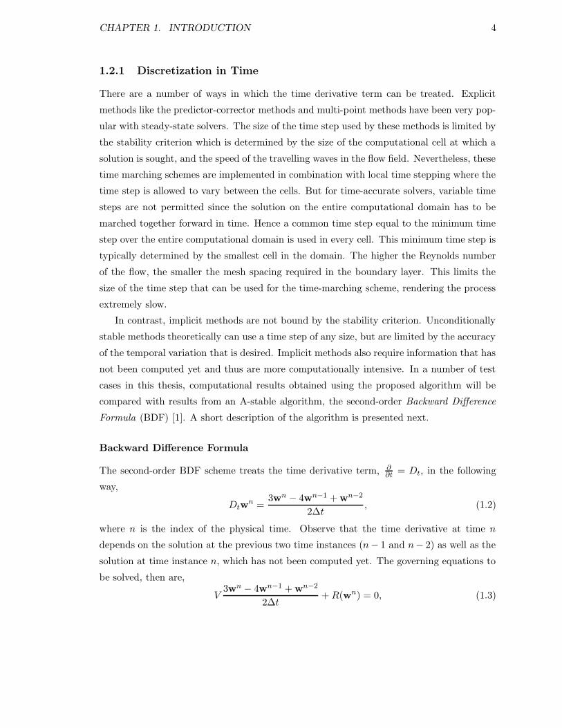
in predicting the amplitude and phase of the periodic solution. Figure 1.1 plots the real
and imaginary parts of k′∆t as a function of k∆t. The plot with the real component also
depicts the linear curve (typical of spectral operators) that k ′∆t should match closely for
accurately capturing as many wavenumbers as possible.
According to the sampling theorem [5], a spectral operator would require at least two
points per wavelength to capture the signal exactly. Hence the wavenumber and number of
CHAPTER 1. INTRODUCTION 7
0 0.5 1 1.5 2 2.5 30
0.5
1
1.5
2
2.5
3
k∆t
Real
(k’∆
t) Real(k’∆t)
k∆t
N=4
N=8
N=16
(a) Real component
0 0.5 1 1.5 2 2.5 30
0.5
1
1.5
2
2.5
3
3.5
4
Imag
(|k’∆
t|)
Imag(|k’∆t|)
N=4
N=8
k∆t
(b) Imaginary component
Figure 1.1: Modified wave number analysis for the second-order BDF scheme
points (N) used to discretize a signal with time period T are closely related by,
N =T
∆t=
2π
k∆t.
Note from the figure that k∆t ranges from 0 to π. k∆t = π corresponds to N = 2, the
minimum number of points per wavelength required by a spectral operator. Figure 1.1
essentially depicts the capability of the BDF scheme to accurately represent the derivative
of a signal with various amounts of resolution. The deviation from the exact representation
(linear curve in the real component and zero in the imaginary component) by the BDF
operator becomes significant for N < 16 (N = 16 corresponds to 5% error in the real
component and 0.5% error in the imaginary component). This implies that while a spectral
operator would require 2 points per wavelength, the BDF operator requires at least 16
points per wavelength for reasonable accuracy.
The topic of this thesis is developing algorithms for time-periodic unsteady flows. As
explained before, the dual-time stepping Backward Difference Formula can be used for
any unsteady problem, and is not restricted to time-periodic problems. With respect to
accuracy, it has also been shown that for a periodic problem, a spectral operator for the
time derivative term would score far better than the BDF scheme with the same number
of time “grid” points. Another advantage of using spectral based methods is that the
CHAPTER 1. INTRODUCTION 8
−1.5 −1 −0.5 0 0.5 1 1.5
−0.1
−0.05
0
0.05
0.1
0.15
Angle of Attack (α)
Coef
ficie
nt o
f Lift
(Cl)
Initial Solution
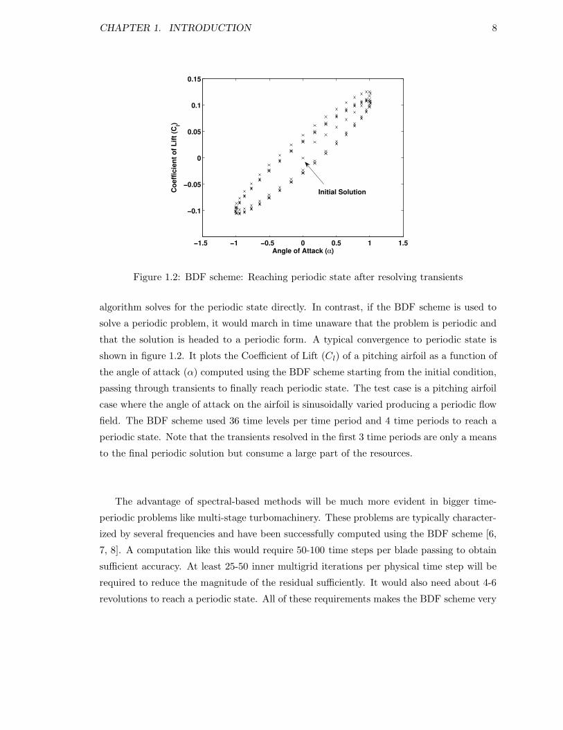
Figure 1.2: BDF scheme: Reaching periodic state after resolving transients
algorithm solves for the periodic state directly. In contrast, if the BDF scheme is used to
solve a periodic problem, it would march in time unaware that the problem is periodic and
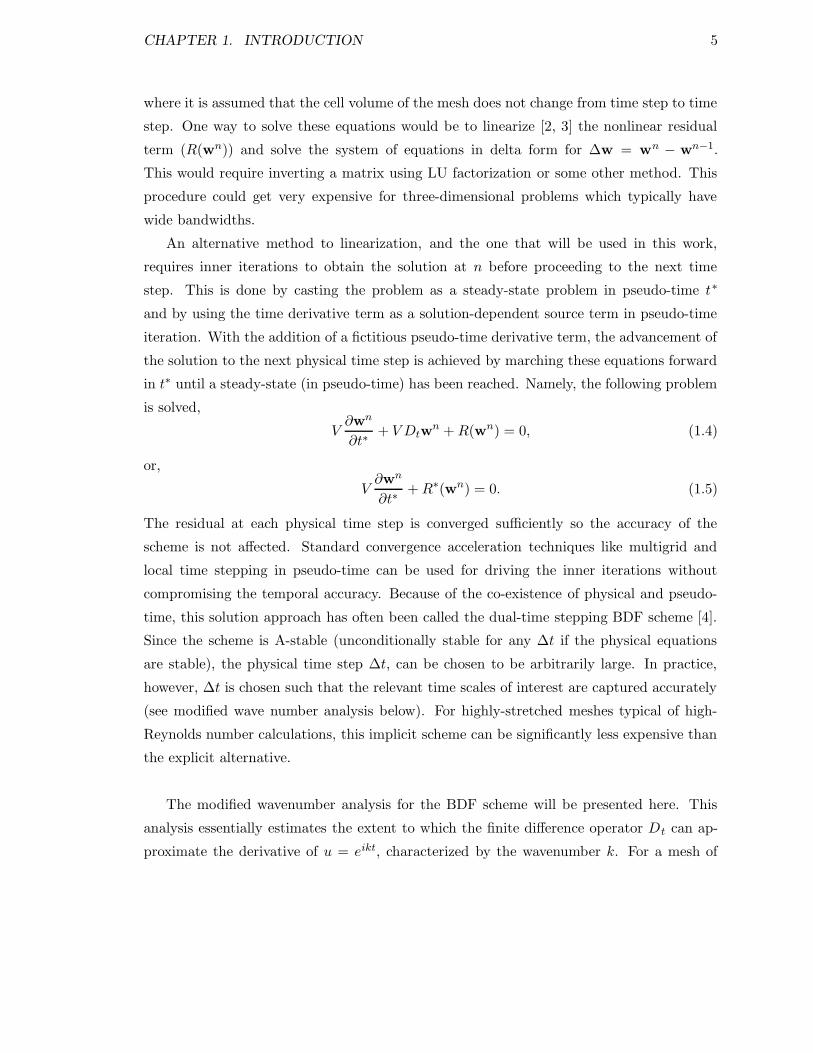
that the solution is headed to a periodic form. A typical convergence to periodic state is
shown in figure 1.2. It plots the Coefficient of Lift (Cl) of a pitching airfoil as a function of
the angle of attack (α) computed using the BDF scheme starting from the initial condition,
passing through transients to finally reach periodic state. The test case is a pitching airfoil
case where the angle of attack on the airfoil is sinusoidally varied producing a periodic flow
field. The BDF scheme used 36 time levels per time period and 4 time periods to reach a
periodic state. Note that the transients resolved in the first 3 time periods are only a means
to the final periodic solution but consume a large part of the resources.
The advantage of spectral-based methods will be much more evident in bigger time-
periodic problems like multi-stage turbomachinery. These problems are typically character-
ized by several frequencies and have been successfully computed using the BDF scheme [6,
7, 8]. A computation like this would require 50-100 time steps per blade passing to obtain
sufficient accuracy. At least 25-50 inner multigrid iterations per physical time step will be
required to reduce the magnitude of the residual sufficiently. It would also need about 4-6
revolutions to reach a periodic state. All of these requirements makes the BDF scheme very
CHAPTER 1. INTRODUCTION 9
expensive for turbomachinery applications.
1.3 Past Efforts in Time-Periodic Unsteady Algorithms
The concept of using Fourier-based methods in time to solve a time-periodic problem is
a fairly established notion. The idea, however, has evolved over the last two decades and
has been heavily influenced by the computing power available. These methods are broadly
termed the Frequency-Domain methods, and have gained widespread popularity in aeroe-
lastic applications.
In their earliest forms, they were used in combination with time-linearized governing
equations. The flow variables were split into a steady part and an unsteady part that was
assumed to be small compared to the mean. Second and higher order terms arising from the
nonlinear equations would be dropped resulting in the steady flow equations and another set
of linear constant-coefficient partial differential equations for the unsteady perturbations.
The steady flow equations would be solved first and then used to construct the constant
coefficients in the equations governing the unsteady component. These unsteady equations
were cast in complex harmonic form leading to a set of equations decoupled for each mode
comprising the harmonic content of the unsteady variation [9, 10]. The computational
requirements for this treatment were very low and also the storage demands were minimal.
This was the case because the various modes were decoupled, and so it was not necessary
that all of them be solved/stored simultaneously. However, solutions to problems were not
predicted well when significant nonlinear effects like shocks were present, and where energy
exchange between different modes was of importance.
Adamczyk [11] proposed a method where the time variation of the flow variables is split
in a different way. The unsteady perturbations were no longer assumed to be small. The flow
variables were split into a time-averaged part and an unsteady part. Due to the nonlinear
nature of the momentum and energy equations, the time-averaging generated extra terms
called deterministic stress terms. These terms were modeled to provide closure. Once the
time-averaged solution had been obtained, these were used to solve the linear equations
for the unsteady perturbations. This procedure did include some nonlinear effects but not
all of them. Also the interaction between the time-average and the unsteady modes was
obvious, but not the interaction between different modes.
CHAPTER 1. INTRODUCTION 10
In order to resolve all the nonlinear effects, the nonlinear harmonic method was pro-
posed by He [12] and further developed for aeroelastic [13, 14] applications and blade-row
interactions [15]. The flow variables were again decomposed into a time-averaged part and
an unsteady part leading to two sets of equations, one for each part. The unsteady part was
obtained by balancing harmonic terms for each frequency. In this procedure, the determinis-
tic stress terms were not modeled anymore. The two sets of equations were interdependent:
the time-averaged equations depended on the perturbations to compute the extra terms,
and the unsteady perturbation equations depended on the time-averaged solution for their
Jacobian matrices. Hence these were solved iteratively until the whole system converged.
The Harmonic Balance method used by Hall et al. has over the years changed its
form as new methodologies developed and more computing resources became available.
The method was first used as a frequency domain technique for linearized unsteady Euler
equations [16, 17]. The first few applications were oscillating cascades and gust response
problems [18, 19]. More recently, the group has pursued full nonlinear and time domain
techniques for the simulation of flutter and multi-stage turbomachinery [20, 21].
McMullen et al. [22, 23] proposed the Non-Linear Frequency Domain (NLFD) method
which solves for the full nonlinear Euler/RANS equations in the frequency domain. All
the flow variables and their corresponding residuals are cast in harmonic form such that
equation (1.1) is transformed to,
V ikwk + Rk = 0.
for each wavenumber/frequency corresponding to k. The equations are not really decoupled
for each mode k. The nonlinear residual term Rk cannot be evaluated directly from wk so
R(wn) is computed from wn and then Fourier transformed to get Rk. But, note that the
Fourier transform operator requires R(w) at all discrete time “grid” points to compute Rk
hence coupling all the modes. First of all, the storage needs are larger since the solution at
all time levels will have to be stored and the computational effort is higher since at least two
Fourier transformations are required every iteration to transform the residuals. However,
all nonlinear effects are accounted for in this method.
CHAPTER 1. INTRODUCTION 11
1.3.1 Past Efforts for Turbomachinery Applications
One of the major applications for which the algorithms proposed in this thesis has been
implemented for is the computation of Turbomachinery flows. A short description of the
various methods used in the turbomachinery field will be appropriate here.
Full-scale time-dependent calculations for unsteady turbomachinery flows are still too
expensive to be suitable for daily design purposes. As explained in Section 1.2.1, a time
accurate calculation using the dual-time stepping BDF scheme for a multi-stage turboma-
chine [6, 7, 8] could be prohibitively expensive. This time-marching scheme can theoretically
take time steps of arbitrary size due to its A-stable nature, but is limited in the time step
size by the requirement on accuracy, such that the relevant time scales are captured. This
scheme resolves all the transients, which typically have very long decay rates, before reaching
a periodic steady-state.
Different variations of reduced-order models have been used over the years in order
to realize fast turn-around times. The simplest of them for turbomachinery problems is
the mixing-plane approach [24], which is a steady approximation to an unsteady problem.
The size of the spatial problem is reduced to a single passage in each blade row, and
a steady computation is carried out in each row. At the interface between blade rows,
a circumferential average of the flow variables is passed to the neighbor: all unsteady
interactions are ignored.
The BDF and Frequency Domain methods do accommodate unsteady interactions but
often include other approximations to lower computational costs. The BDF scheme is
frequently used in combination with scaled geometries (the blade counts of the blade rows
are modified such that a representative periodic fraction of the annulus is produced while
maintaining solidity), such that a periodic fraction of the annulus is solved instead of the
whole annulus. In the Frequency Domain methods, the size of the spatial problem is often
confined to a single blade passage per blade row using phase shifted boundary conditions
on the upper and lower azimuthal locations of the single passage computational domain.
These phase-lag conditions have changed their form from the first “direct store” method
proposed by Erdos et al. [25, 26] through the time-inclination method by Giles [27], to the
Fourier series based “shape correction method” by He [28, 29]. They have been extensively
used in turbomachinery analysis codes like MSU-TURBO [30].
Ekici and Hall [31] proposed the mixed time-domain / frequency-domain Harmonic Bal-
ance method to solve the full nonlinear RANS equations for multi-stage turbomachinery
CHAPTER 1. INTRODUCTION 12
problems. The distinguishing feature of this reduced-order model (compared with the orig-
inal Harmonic Balance method [19]) is that only a specified set of frequencies (comprising
combinations of the neighbor’s blade passing frequencies) is resolved in each blade row.
Unlike single stage problems, in multi-stage machinery (each blade row has more than one
neighbor), this would amount to resolving frequencies that are not multiples of a single
fundamental frequency. Solution over a smaller time span and a smaller computational
domain yields considerable computational savings. However, the transfer of information at
the interface between blade rows is carried out in the frequency space via an exchange of
Fourier coefficients. This requires a radially matched grid for the computation, which might
be restrictive and also can be regarded as a drawback, since an extension to unstructured
grids will not be straightforward.
1.4 Current Approach: Fourier-Based Time Domain Tech-
niques
The main objective of this work is to compute the solution to time-periodic problems us-
ing Fourier-based algorithms that can take advantage of the periodicity of the problem.
This way, the periodic solution can be directly obtained gaining immensely on efficiency,
instead of resolving inconsequential transients that are typical of time-marching schemes.
As mentioned in the previous section, traditionally, Fourier-based methods cast the govern-
ing equations in the frequency domain. The transformation of the variables to and from
the frequency domain in a nonlinear framework somewhat restricts the ease with which an
already existing solver can be modified to suit the simulation of periodically unsteady flows.
The core of the new algorithm, the Time Spectral Method, stems from these ideas. It is
a Fourier-based algorithm, but it solves the governing equations purely in the time domain.
The algorithm discretizes the time derivative term in equation (1.1) and transforms it into
a matrix-vector product that is added to the spatial discrete part. The matrix-vector
product couples the variables at all time levels in the periodic interval. The variables at
every time level are simultaneously iterated until the periodic steady-state is reached, unlike
time-marching schemes. The addition of the time derivative matrix-vector product to the
spatial part of the residual results in a modified residual term which can then be driven to
zero by introducing a pseudo-time derivative and iterating to steady-state in pseudo-time.
This facilitates the use of an already existing solver, that can benefit from state-of-the-art
CHAPTER 1. INTRODUCTION 13
methodologies like multigrid, local time stepping in pseudo-time, parallelization in space
etc.
In order to take advantage of the periodicity of the problem, the Time Spectral method
is provided indirectly (through the Fourier basis) with the time period or frequency of un-
steadiness of the problem. Furnishing the time period is fairly straightforward in cases
where the frequency is predetermined, mostly due to the geometry or motion of the body.
It is not as easy when the frequency is not known a priori. In such cases, the Time Spec-
tral method is used in combination with a gradient-based approach, based on McMullen’s
GBVTP method [23] that was proposed with the NLFD technique. Using this approach,
starting from an initial guess of the time period, the exact frequency of unsteadiness is
computed iteratively as part of the solution.
The benefits of the Time Spectral method over conventional time-marching schemes will
be much more evident when applied to practical three-dimensional time-periodic problems.
To this effect, turbomachinery applications have been chosen in this work to demonstrate
the efficiency and accuracy of the proposed algorithm. The Time Spectral method is mod-
ified so that it can be applied to periodic sector problems (this might require a scaling of
the geometry) in a Cartesian framework. Traditionally, due to the wide popularity of Fast
Fourier Transforms (FFT), Fourier-based methods have used an even (more precisely 2n,
although other FFTs do exist that use number of points equal to a product of prime num-
bers) number of grid points. The Time Spectral method does not use FFTs and hence does
not suffer from this restriction. The algorithm has both an even and an odd formulation,
but the even formulation has proved to permit odd-even decoupling of the time levels, which
could destabilize the algorithm in cases where the unsteady effects are predominant.
Further improvements in computational efficiency can be realized for multi-stage tur-
bomachinery problems using a reduced-order Harmonic Balance method similar to the one
proposed by Kick and Hall [31]. The key difference between the two methodologies is that
the current approach is implemented purely in the time domain, whereas the one proposed
by Ekici and Hall is a mixed time domain / frequency domain approach which requires the
extra storage of Fourier coefficients and transformations using Fourier transforms. Only
a specified set of dominant frequencies in each blade row is resolved in the time domain
reduced-order Harmonic Balance method, similar to its frequency domain counterpart. So-
lutions are also sought over a smaller time span and a smaller computational domain com-
pared to the Time Spectral method, leading to tremendous savings. However, the time
CHAPTER 1. INTRODUCTION 14
domain technique, suffers from aliasing errors that can destabilize a computation. De-
aliasing procedures have to be performed to “cleanse” the solution off these high frequency
errors.
1.5 Dissertation Outline
The rest of this dissertation delves into the details of the proposed algorithms and demon-
strates the validity of its accuracy and efficiency through test cases that compare results
obtained using them with experimental and other numerical results where appropriate.
Chapter 2 outlines the derivation of the Time Spectral method for even and odd numbers
of discretization points in time. The derivation of an analytic expression for the terms
of the time derivative operator is presented from basic principles of Fourier transforms.
The performance of the method is demonstrated using simple two- and three-dimensional
validation test cases. These results verify that a small number of modes/time levels are
sufficient to capture forced response problems.
The Time Spectral method is modified for predicting time-periodic flows where the
periodicity is not enforced and hence is not known a priori. The gradient-based approach
used to iteratively solve for the time period is illustrated in Chapter 3. The method is tested
for two-dimensional laminar vortex shedding cases and results compared with experimental
and numerical data.
The Time Spectral method and the time-domain reduced-order Harmonic Balance method
are applied to turbomachinery problems in Chapter 4. Three-dimensional results are pre-
sented for a single stage compressor and two-dimensional results for a multi-stage compres-
sor. These results are compared with results from conventional time-accurate computations.
Accuracy and cost comparisons are presented and the capabilities and limitations of each
of these algorithms are discussed.
Chapter 5, finally surveys the results from all the chapters and summarizes them. Future
directions for research and improvements to the current work are also suggested.
Chapter 2
Time Spectral Method
This chapter addresses periodic unsteady problems for which the frequency of unsteadiness
is known a priori. Such is the case when the boundary conditions force unsteadiness at
predetermined frequencies. Typical examples of this class of unsteady problems are rotor-
stator combinations in turbomachinery, helicopter rotors in forward flight and wind turbines,
to name a few. In all these examples, the flow is periodic with the time period of the moving
parts. In other words, the frequency content of the flow field is composed of the excitation
frequency and its harmonics.
2.1 Time Derivative Term as a Matrix Operator
The core of the Time Spectral algorithm lies in the representation of the unsteady variation
of the solution in the form of a Fourier series. A Fourier series representation essentially
forces the solution to vary in a periodic manner. Therefore, the algorithm directly solves
for the periodic state without having to resolve the transients.
Every flow variable in every computational cell in the mesh, is assumed to vary peri-
odically. Consider one such flow variable in a single computational cell. The periodic time
variation of this variable at N equally spaced time intervals form the elements of the vector,
U∗,
U∗ = [U∗
t0, U∗
t1, · · · , U ∗
tN−1]T .
15
CHAPTER 2. TIME SPECTRAL METHOD 16
If T is the time period of U∗, the forward Fourier transform of the solution is given by,
Uk =1
N
N−1∑
n=0
U∗
ne−i(k 2πT
)tn , (2.1)
where n is the index of the time level, k the wavenumber, and Uk is the Fourier coefficient
corresponding to the wavenumber k,
U = [U0, U1, U2, · · · , UK , U−K , · · · , U−1]T .
K is the highest wave number that N (odd) time instances can accommodate and is called
the Nyquist frequency, given by
KNyquist =N − 1
2.
Each wavenumber k corresponds to a frequency,
fk = k2π
T.
It should be noted from the above equation that the frequency set,
f = [f0, f1, · · · , fK , f−K , · · · , f−1]T (2.2)
is such that f0 = 0 and f−K = −fK ensuring a real U ∗. Hence there are only K independent
frequencies represented by N = 2K + 1 time levels. (this is another way of explaining the
Nyquist frequency.) In addition, f2 = 2f1, f3 = 3f1, · · · , fk = kf1. Thus the frequency
content of the solution U∗ consists of one fundamental frequency f1 = 2πT
, and K−1 higher
harmonics.
The Fourier transform in equation (2.1) can also be expressed in terms of the Fourier
matrix E as,
U = EU∗,
where
Ek,n =1
Ne−ifktn . (2.3)
CHAPTER 2. TIME SPECTRAL METHOD 17
The inverse Fourier transform is simply the inverse operation using E−1 which also has an
analytic expression,
E−1k,n = eifktn .
The main focus of this thesis is the treatment of the time derivative term DtU∗ in the
governing set of equations. Following a number of mathematical tricks in combination with
the Fourier matrices, an expression for the Dt operator can be arrived at as follows:
DtU∗ = Dt(E
−1EU∗) = Dt(E−1U).
Since U is independent of time, the Dt operates only on E−1 so that,
DtU∗ = E−1DU = E−1DEU∗.
Hence,
Dt = E−1DE, (2.4)
where the matrix D is a diagonal matrix whose elements are,
Dkk = ifk.
A simpler form of this combined operator is presented in Appendix B where Dt is rewritten
as a matrix operator whose elements are
doddlj =
12(−1)l−jcosec(π(l−j)
N) : l 6= j
0 : l = j
devenlj =
12(−1)l−jcot(π(l−j)
N) : l 6= j
0 : l = j
for odd and even N respectively. These expressions for the time derivative operator, Dt,
can be rewritten after a change of indices as,
doddm =
12(−1)m+1cosec(πm
N) : m 6= 0
0 : m = 0(2.5)
CHAPTER 2. TIME SPECTRAL METHOD 18
devenm =
12(−1)m+1cot(πm
N) : m 6= 0
0 : m = 0(2.6)
It is clear from equation (2.5) and 2.6 that the matrix operator is a central difference
operator with zeros on the diagonals and d−m = −dm, i.e.,
Doddt =
0 dodd1 · · · dodd
N−1
2
−doddN−1
2
· · · −dodd1
−dodd1 0 dodd
1 dodd2 · · · · · · −dodd
2...
......
......
......
dodd1 dodd
2 · · · · · · −dodd2 −dodd
1 0
(2.7)
Devent =
0 deven1 · · · deven
N2−1
0 −devenN2−1
· · · −deven1
−deven1 0 deven
1 deven2 · · · 0 · · · −deven
2...
......
......
......
...
deven1 deven
2 · · · 0 · · · −deven2 −deven
1 0
(2.8)
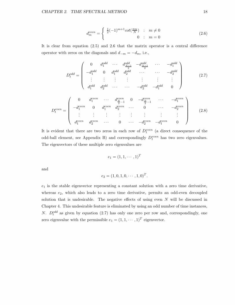
It is evident that there are two zeros in each row of Devent (a direct consequence of the
odd-ball element, see Appendix B) and correspondingly Devent has two zero eigenvalues.
The eigenvectors of these multiple zero eigenvalues are
e1 = (1, 1, · · · , 1)T
and
e2 = (1, 0, 1, 0, · · · , 1, 0)T .
e1 is the stable eigenvector representing a constant solution with a zero time derivative,
whereas e2, which also leads to a zero time derivative, permits an odd-even decoupled
solution that is undesirable. The negative effects of using even N will be discussed in
Chapter 4. This undesirable feature is eliminated by using an odd number of time instances,
N . Doddt as given by equation (2.7) has only one zero per row and, correspondingly, one
zero eigenvalue with the permissible e1 = (1, 1, · · · , 1)T eigenvector.

CHAPTER 2. TIME SPECTRAL METHOD 19
The time derivative term has now been transformed into a matrix vector product, i.e.,
∂U∗
t0
∂t∂U∗
t1
∂t...
∂U∗
tN−1
∂t
= Dt
U∗
t0
U∗
t1...
U∗
tN−1
. (2.9)
Equation (2.9) implies that the derivative at any time instance depends on all other time
instances coupled together by the full matrix operator, Dt. This requires the storage of
every variable at every time level on the entire computational domain, so that the variables
at all time levels can be iterated simultaneously to reach a periodic state. Essentially, the
Time Spectral method is a ”four-dimensional” space-time representation, and its memory
requirements relative to a time-marching method scale as n4 versus n3, where n is roughly
the number of “grid” points in each dimension. This feature could prove to be prohibitive
in cases where a high harmonic of the fundamental is required to be resolved and hence
a correspondingly large N be used for the computation. This will be further discussed in
Chapter 4 in the context of turbomachinery applications.
2.2 Results
The efficiency and accuracy of the Time Spectral method will be illustrated in this section
through two- and three-dimensional validation test cases. The solver used for this purpose
is a conservative cell-centered finite volume scheme. A full W-cycle multigrid [32] algorithm
is used for accelerating convergence, in which a pseudo-time step with a five-stage Runge-
Kutta scheme is performed at each level. The Jameson-Schmidt-Turkel (JST) [33] scheme
is used as the artificial dissipation scheme where blended first and third order dissipation
terms are introduced to suppress spurious modes and ensure stability. A thorough descrip-
tion of this scheme is provided by Jameson [34, 35]. The algebraic Baldwin-Lomax [36]
turbulence model is used to model eddy viscosity in the unsteady RANS computations
(note: the unsteady effects on the turbulence quantities are neglected). Parallelization in
space is facilitated due to the explicit nature of the time advancement scheme. The Message
Passing Interface (MPI) [37] standard is used for the parallel implementation of the three-
dimensional unsteady RANS equations in the FLO107 (Single block structured cell-centered
finite volume solver for the solution of RANS equations on three-dimensional wings in the
CHAPTER 2. TIME SPECTRAL METHOD 20
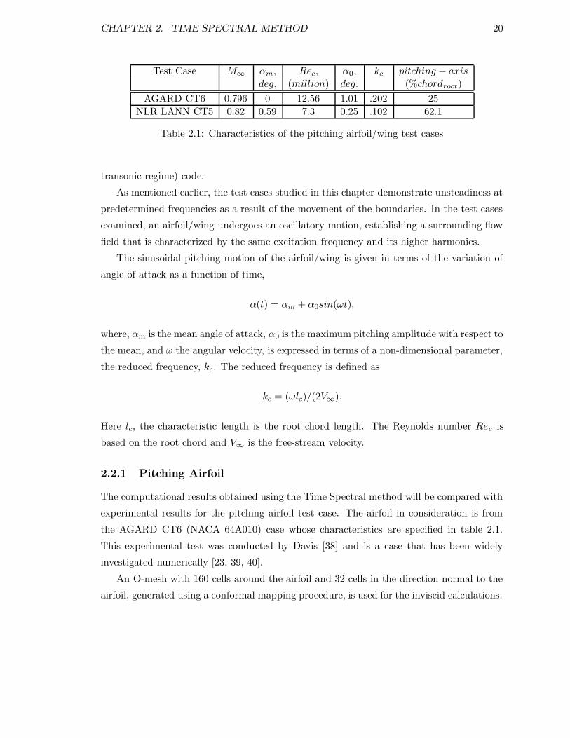
Test Case M∞ αm, Rec, α0, kc pitching − axisdeg. (million) deg. (%chordroot)
AGARD CT6 0.796 0 12.56 1.01 .202 25
NLR LANN CT5 0.82 0.59 7.3 0.25 .102 62.1
Table 2.1: Characteristics of the pitching airfoil/wing test cases
transonic regime) code.
As mentioned earlier, the test cases studied in this chapter demonstrate unsteadiness at
predetermined frequencies as a result of the movement of the boundaries. In the test cases
examined, an airfoil/wing undergoes an oscillatory motion, establishing a surrounding flow
field that is characterized by the same excitation frequency and its higher harmonics.
The sinusoidal pitching motion of the airfoil/wing is given in terms of the variation of
angle of attack as a function of time,
α(t) = αm + α0sin(ωt),
where, αm is the mean angle of attack, α0 is the maximum pitching amplitude with respect to
the mean, and ω the angular velocity, is expressed in terms of a non-dimensional parameter,
the reduced frequency, kc. The reduced frequency is defined as
kc = (ωlc)/(2V∞).
Here lc, the characteristic length is the root chord length. The Reynolds number Rec is
based on the root chord and V∞ is the free-stream velocity.
2.2.1 Pitching Airfoil
The computational results obtained using the Time Spectral method will be compared with
experimental results for the pitching airfoil test case. The airfoil in consideration is from
the AGARD CT6 (NACA 64A010) case whose characteristics are specified in table 2.1.
This experimental test was conducted by Davis [38] and is a case that has been widely
investigated numerically [23, 39, 40].
An O-mesh with 160 cells around the airfoil and 32 cells in the direction normal to the
airfoil, generated using a conformal mapping procedure, is used for the inviscid calculations.
CHAPTER 2. TIME SPECTRAL METHOD 21
NACA 64A010 GRID 160 X 32
NACA CT6 AIRFOIL GRID 256 X 64
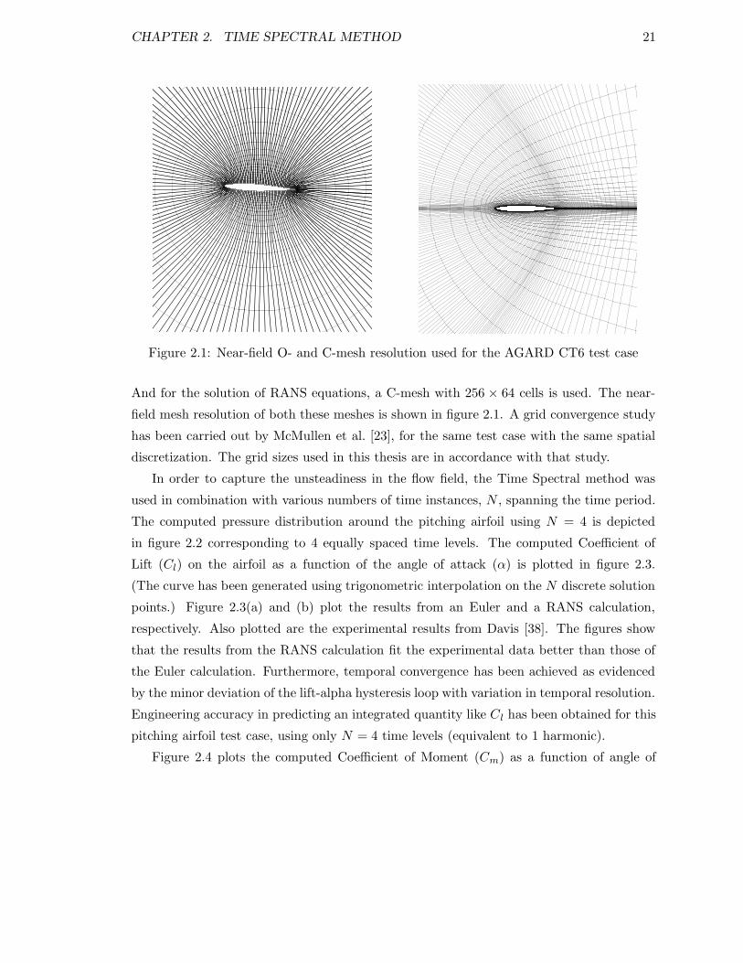
Figure 2.1: Near-field O- and C-mesh resolution used for the AGARD CT6 test case
And for the solution of RANS equations, a C-mesh with 256 × 64 cells is used. The near-
field mesh resolution of both these meshes is shown in figure 2.1. A grid convergence study
has been carried out by McMullen et al. [23], for the same test case with the same spatial
discretization. The grid sizes used in this thesis are in accordance with that study.
In order to capture the unsteadiness in the flow field, the Time Spectral method was
used in combination with various numbers of time instances, N , spanning the time period.
The computed pressure distribution around the pitching airfoil using N = 4 is depicted
in figure 2.2 corresponding to 4 equally spaced time levels. The computed Coefficient of
Lift (Cl) on the airfoil as a function of the angle of attack (α) is plotted in figure 2.3.
(The curve has been generated using trigonometric interpolation on the N discrete solution
points.) Figure 2.3(a) and (b) plot the results from an Euler and a RANS calculation,
respectively. Also plotted are the experimental results from Davis [38]. The figures show
that the results from the RANS calculation fit the experimental data better than those of
the Euler calculation. Furthermore, temporal convergence has been achieved as evidenced
by the minor deviation of the lift-alpha hysteresis loop with variation in temporal resolution.
Engineering accuracy in predicting an integrated quantity like Cl has been obtained for this
pitching airfoil test case, using only N = 4 time levels (equivalent to 1 harmonic).
Figure 2.4 plots the computed Coefficient of Moment (Cm) as a function of angle of
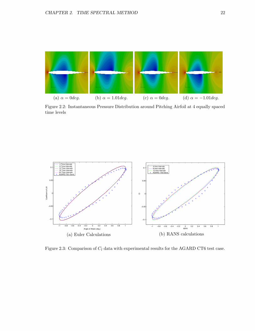
CHAPTER 2. TIME SPECTRAL METHOD 22
(a) α = 0deg. (b) α = 1.01deg. (c) α = 0deg. (d) α = −1.01deg.
Figure 2.2: Instantaneous Pressure Distribution around Pitching Airfoil at 4 equally spacedtime levels
−1 −0.8 −0.6 −0.4 −0.2 0 0.2 0.4 0.6 0.8 1
−0.1
−0.05
0
0.05
0.1
Angle of Attack (deg.)
Coef
ficie
nt o
f Lift
4 Time Intervals 8 Time Intervals12 Time Intervals16 Time Intervals24 Time IntervalsAGARD:702−Davis
(a) Euler Calculations
−1 −0.8 −0.6 −0.4 −0.2 0 0.2 0.4 0.6 0.8 1
−0.1
−0.05
0
0.05
0.1
alpha
Cl
4 time intervals8 time intervals12 time intervalsAGARD−702:Davis
(b) RANS calculations
Figure 2.3: Comparison of Cl data with experimental results for the AGARD CT6 test case.
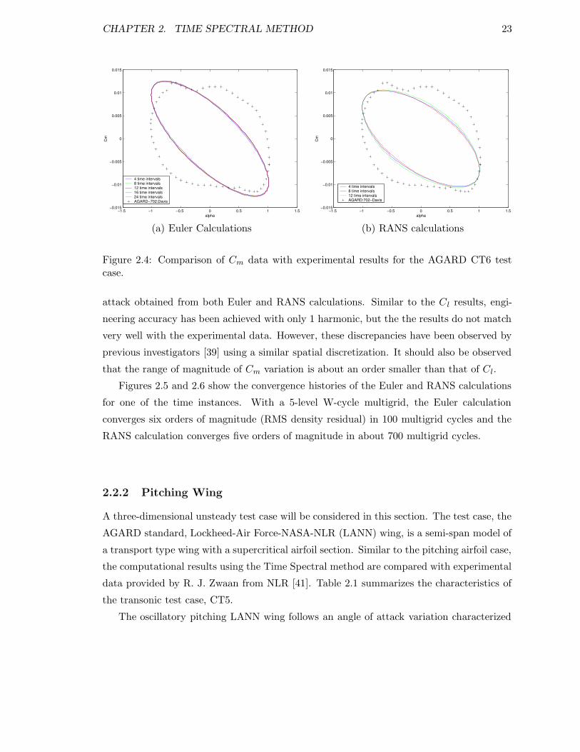
CHAPTER 2. TIME SPECTRAL METHOD 23
−1.5 −1 −0.5 0 0.5 1 1.5−0.015
−0.01
−0.005
0
0.005
0.01
0.015
alpha
Cm
4 time intervals8 time intervals12 time intervals16 time intervals24 time intervalsAGARD−702:Davis
(a) Euler Calculations
−1.5 −1 −0.5 0 0.5 1 1.5−0.015
−0.01
−0.005
0
0.005
0.01
0.015
alpha
Cm
4 time intervals8 time intervals12 time intervalsAGARD:702−Davis
(b) RANS calculations
Figure 2.4: Comparison of Cm data with experimental results for the AGARD CT6 testcase.
attack obtained from both Euler and RANS calculations. Similar to the Cl results, engi-
neering accuracy has been achieved with only 1 harmonic, but the the results do not match
very well with the experimental data. However, these discrepancies have been observed by
previous investigators [39] using a similar spatial discretization. It should also be observed
that the range of magnitude of Cm variation is about an order smaller than that of Cl.
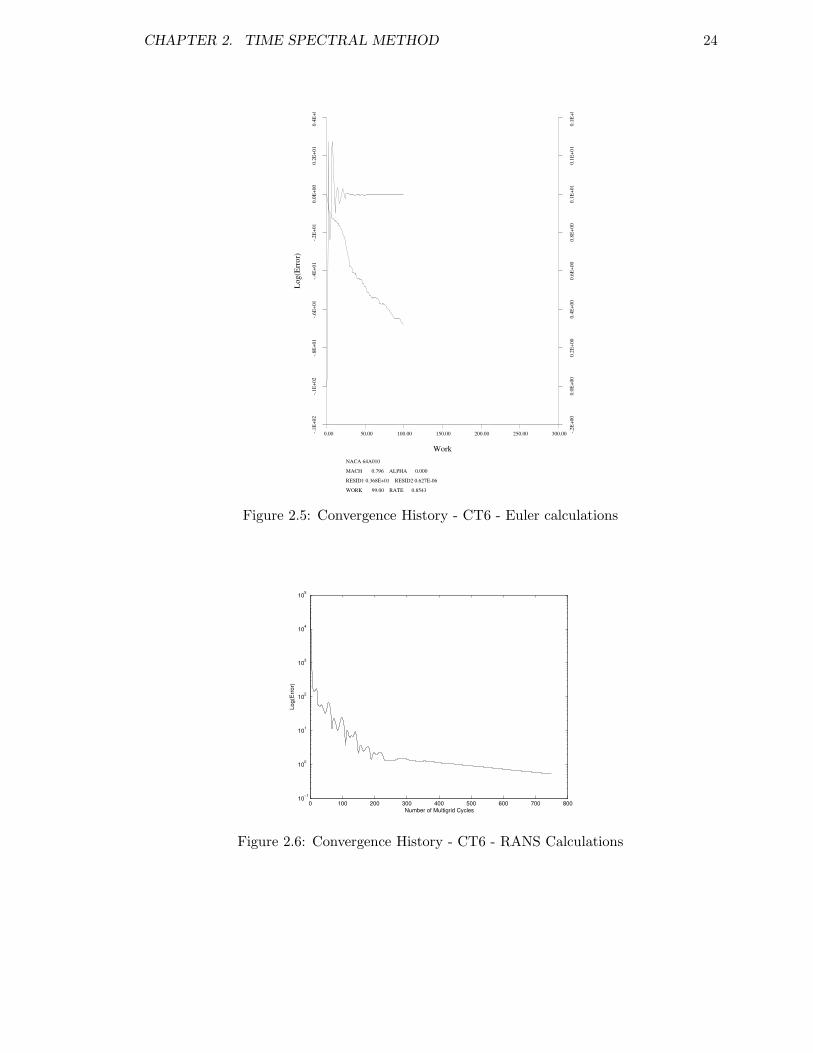
Figures 2.5 and 2.6 show the convergence histories of the Euler and RANS calculations
for one of the time instances. With a 5-level W-cycle multigrid, the Euler calculation
converges six orders of magnitude (RMS density residual) in 100 multigrid cycles and the
RANS calculation converges five orders of magnitude in about 700 multigrid cycles.
2.2.2 Pitching Wing
A three-dimensional unsteady test case will be considered in this section. The test case, the
AGARD standard, Lockheed-Air Force-NASA-NLR (LANN) wing, is a semi-span model of
a transport type wing with a supercritical airfoil section. Similar to the pitching airfoil case,
the computational results using the Time Spectral method are compared with experimental
data provided by R. J. Zwaan from NLR [41]. Table 2.1 summarizes the characteristics of
the transonic test case, CT5.
The oscillatory pitching LANN wing follows an angle of attack variation characterized
CHAPTER 2. TIME SPECTRAL METHOD 24
NACA 64A010
MACH 0.796 ALPHA 0.000
RESID1 0.368E+01 RESID2 0.627E-06
WORK 99.00 RATE 0.8543
GRID 160X 32
0.00 50.00 100.00 150.00 200.00 250.00 300.00
Work
-.1E+
02-.1
E+02
-.8E+
01-.6
E+01
-.4E+
01-.2
E+01
0.0E
+00
0.2E
+01
0.4E
+01
Log(
Erro
r)
-.2E+
000.
0E+0
00.
2E+0
00.
4E+0
00.
6E+0
00.
8E+0
00.
1E+0
10.
1E+0
10.
1E+0
1
Nsu
p
Figure 2.5: Convergence History - CT6 - Euler calculations
0 100 200 300 400 500 600 700 80010−1
100
101
102
103
104
105
Number of Multigrid Cycles
Log(
Erro
r)
Figure 2.6: Convergence History - CT6 - RANS Calculations
CHAPTER 2. TIME SPECTRAL METHOD 25
0 0.1 0.2 0.3 0.4 0.5 0.6 0.7 0.8 0.9 1−0.8
−0.6
−0.4
−0.2
0
0.2
0.4
0.6
0.8
1
x/c
−Cp
NLR−Exp LowerNLR−Exp UpperDLR FP+VII NumTS−4 time intervalsTS−8 time intervalsTS−12 time intervals
(a) η = 20%, α = αmean = 0.59 deg.
0 0.2 0.4 0.6 0.8 1−0.8
−0.6
−0.4
−0.2
0
0.2
0.4
0.6
0.8
1
x/c
−Cp
NLR−Exp LowerNLR−Exp UpperDLR FP+VII NumTS−4 time intervalsTS−8 time intervalsTS−12 time intervals
(b) η = 20%, α = αmax = 0.84 deg.
Figure 2.7: Pressure Distribution At 20% Span : Verification with Experimental and a VIINumerical Method
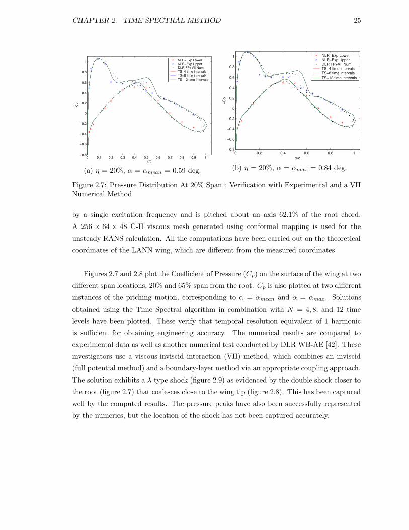
by a single excitation frequency and is pitched about an axis 62.1% of the root chord.
A 256 × 64 × 48 C-H viscous mesh generated using conformal mapping is used for the
unsteady RANS calculation. All the computations have been carried out on the theoretical
coordinates of the LANN wing, which are different from the measured coordinates.
Figures 2.7 and 2.8 plot the Coefficient of Pressure (Cp) on the surface of the wing at two
different span locations, 20% and 65% span from the root. Cp is also plotted at two different
instances of the pitching motion, corresponding to α = αmean and α = αmax. Solutions
obtained using the Time Spectral algorithm in combination with N = 4, 8, and 12 time
levels have been plotted. These verify that temporal resolution equivalent of 1 harmonic
is sufficient for obtaining engineering accuracy. The numerical results are compared to
experimental data as well as another numerical test conducted by DLR WB-AE [42]. These
investigators use a viscous-inviscid interaction (VII) method, which combines an inviscid
(full potential method) and a boundary-layer method via an appropriate coupling approach.
The solution exhibits a λ-type shock (figure 2.9) as evidenced by the double shock closer to
the root (figure 2.7) that coalesces close to the wing tip (figure 2.8). This has been captured
well by the computed results. The pressure peaks have also been successfully represented
by the numerics, but the location of the shock has not been captured accurately.
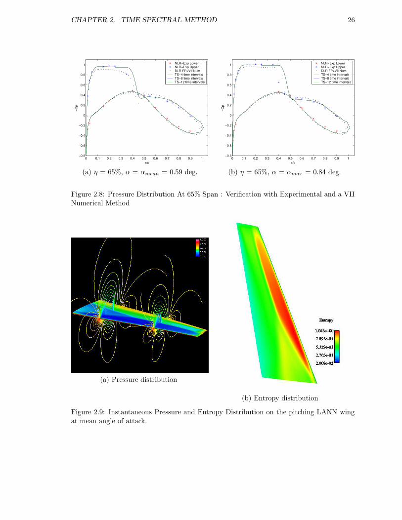
CHAPTER 2. TIME SPECTRAL METHOD 26
0 0.1 0.2 0.3 0.4 0.5 0.6 0.7 0.8 0.9 1−0.8
−0.6
−0.4
−0.2
0
0.2
0.4
0.6
0.8
1
x/c
−Cp
NLR−Exp LowerNLR−Exp UpperDLR FP+VII NumTS−4 time intervalsTS−8 time intervalsTS−12 time intervals
(a) η = 65%, α = αmean = 0.59 deg.
0 0.1 0.2 0.3 0.4 0.5 0.6 0.7 0.8 0.9 1−0.8
−0.6
−0.4
−0.2
0
0.2
0.4
0.6
0.8
1
x/c
−Cp
NLR−Exp LowerNLR−Exp UpperDLR FP+VII NumTS−4 time intervalsTS−8 time intervalsTS−12 time intervals
(b) η = 65%, α = αmax = 0.84 deg.
Figure 2.8: Pressure Distribution At 65% Span : Verification with Experimental and a VIINumerical Method
(a) Pressure distribution
(b) Entropy distribution
Figure 2.9: Instantaneous Pressure and Entropy Distribution on the pitching LANN wingat mean angle of attack.

CHAPTER 2. TIME SPECTRAL METHOD 27
NLR LANN WING UNSTEADY-TIME SPECTRAL
MACH 0.822 ALPHA 0.590
RESID1 0.905E+04 RESID2 0.332E-01
WORK 799.00 RATE 0.9845
GRID 256X64X48
0.00 200.00 400.00 600.00 800.00 1000.00 1200.00
Work
-.1E+
02-.1
E+02
-.8E+
01-.6
E+01
-.4E+
01-.2
E+01
0.0E
+00
0.2E
+01
0.4E
+01
Log(
Erro
r)
-.2E+
000.
0E+0
00.
2E+0
00.
4E+0
00.
6E+0
00.
8E+0
00.
1E+0
10.
1E+0
10.
1E+0
1
Nsu
p
Figure 2.10: Convergence History - LANN Wing - RANS calculation
CHAPTER 2. TIME SPECTRAL METHOD 28
0 20
0.5
1
1.5
2
2.5
3
t/π
α
(a)
−60 −40 −20 0 20 40 6010−20
10−15
10−10
10−5
100
wavenumbers k
Freq
uenc
y Co
nten
t
(b)
Figure 2.11: Temporal Convergence: (a) Variation of angle of attack over one time period(b) Frequency spectrum of this periodic variation
Figure 2.10 shows the convergence history of the RANS calculation for the LANN pitch-
ing wing. With a 4-level W-cycle multigrid, the parallel code converges 5 orders of magni-
tude in 800 multigrid cycles.
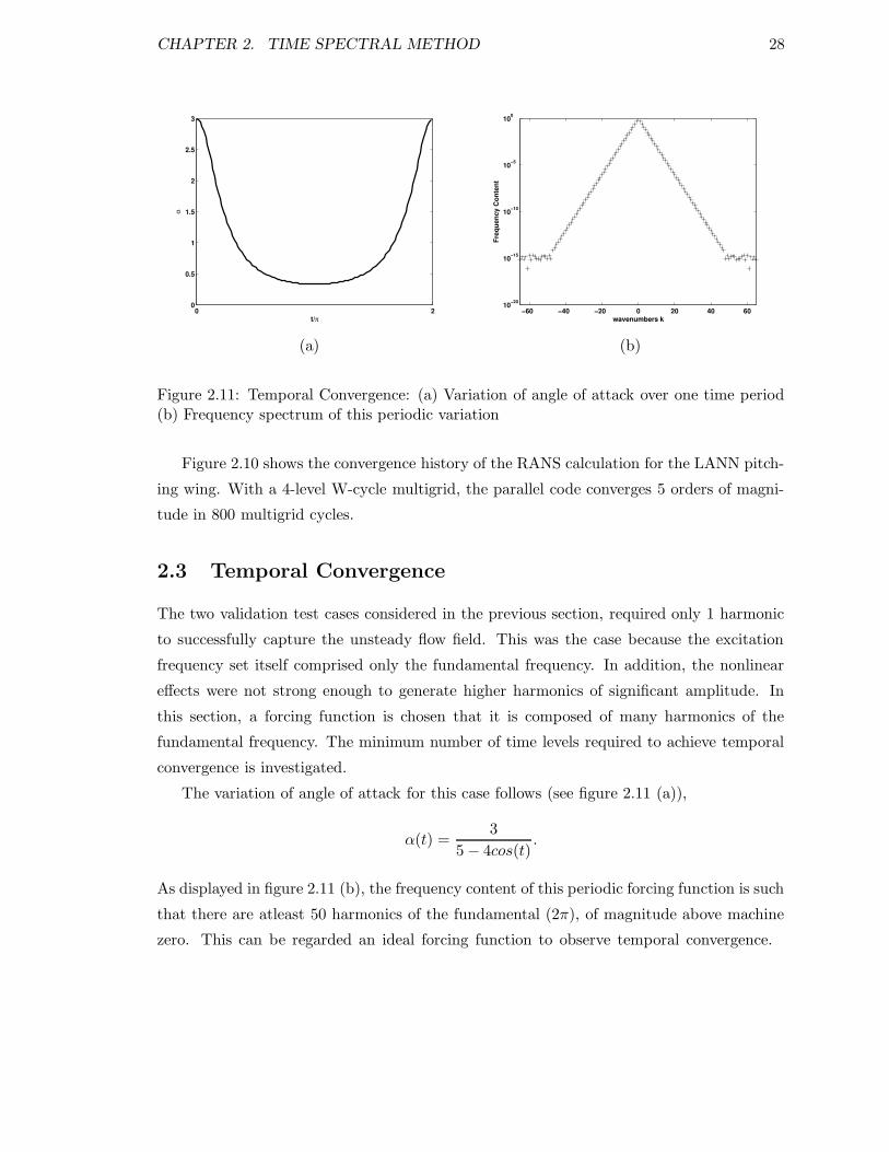
2.3 Temporal Convergence
The two validation test cases considered in the previous section, required only 1 harmonic
to successfully capture the unsteady flow field. This was the case because the excitation
frequency set itself comprised only the fundamental frequency. In addition, the nonlinear
effects were not strong enough to generate higher harmonics of significant amplitude. In
this section, a forcing function is chosen that it is composed of many harmonics of the
fundamental frequency. The minimum number of time levels required to achieve temporal
convergence is investigated.
The variation of angle of attack for this case follows (see figure 2.11 (a)),
α(t) =3
5 − 4cos(t).
As displayed in figure 2.11 (b), the frequency content of this periodic forcing function is such
that there are atleast 50 harmonics of the fundamental (2π), of magnitude above machine
zero. This can be regarded an ideal forcing function to observe temporal convergence.
CHAPTER 2. TIME SPECTRAL METHOD 29
0 0.5 1 1.5 2 2.5 3
0.1
0.2
0.3
0.4
0.5
0.6
Alpha
Cl
4 time intervals8 time intervals12 time intervals16 time intervals20 time intervals24 time intervals
(a) Cl-α plot
0 0.5 1 1.5 2 2.5 3−0.25
−0.2
−0.15
−0.1
−0.05
0
0.05
0.1
0.15
Alpha
Cm
4 time intervals8 time intervals12 time intervals16 time intervals20 time intervals24 time intervals
(b) Cm-α plot
Figure 2.12: Cl-α and Cm-α plots showing temporal convergence
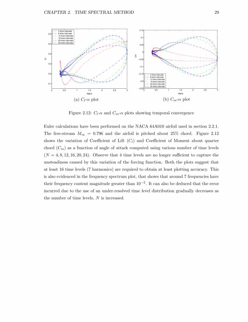
Euler calculations have been performed on the NACA 64A010 airfoil used in section 2.2.1.
The free-stream M∞ = 0.796 and the airfoil is pitched about 25% chord. Figure 2.12
shows the variation of Coefficient of Lift (Cl) and Coefficient of Moment about quarter
chord (Cm) as a function of angle of attack computed using various number of time levels
(N = 4, 8, 12, 16, 20, 24). Observe that 4 time levels are no longer sufficient to capture the
unsteadiness caused by this variation of the forcing function. Both the plots suggest that
at least 16 time levels (7 harmonics) are required to obtain at least plotting accuracy. This
is also evidenced in the frequency spectrum plot, that shows that around 7 frequencies have
their frequency content magnitude greater than 10−2. It can also be deduced that the error
incurred due to the use of an under-resolved time level distribution gradually decreases as
the number of time levels, N is increased.
Chapter 3
Periodic Unsteady Vortex
Shedding Problems
So far, the Time Spectral method has been utilized for the prediction of periodic unsteady
flows where the frequency of unsteadiness was known a priori. This frequency content of
the flow field was a consequence of the time variation of the boundary conditions of the
problem. In Chapter 2, where pitching airfoil/wing test cases were considered, the frequency
of unsteadiness produced in the flow field was composed of the pitching frequency and its
higher harmonics. Chapter 4 will focus on the application of the Time Spectral method to
turbomachinery problems. Here too, the frequency content of the flow field is determined
by the frequency of rotation of the rotors.
This chapter addresses problems which are indeed unsteady in a periodic way, but the
frequency of unsteadiness is not known a priori. The flow conditions and/or the geometry
of the problem establish the flow field. Textbook examples such as wakes behind circular
cylinders and spheres have been studied for years. Understanding such flows is important
even from a practical standpoint in applications such as the reduction of base drag on
automobiles and trucksd.
As explained in Chapter 2, the Time Spectral method uses a Fourier representation in
time. A Fourier series basically fits sine and cosine functions through equally spaced points
on a periodic interval. In order to use the Time Spectral method for the class of problems
considered here, the computation is started with an initial guess of the time period such that
a Fourier series approach can still be used. A gradient-based formulation is then employed
where the time period is corrected iteratively as the residuals are driven to zero. This
30
CHAPTER 3. PERIODIC UNSTEADY VORTEX SHEDDING PROBLEMS 31
procedure is very similar to the Gradient Based Variable Time Period (GBVTP) method
proposed by McMullen et al. [23] in combination with the Nonlinear Frequency Domain
method [22].
3.1 Gradient-based method for computing the Time Period
A steady numerical treatment of a truly unsteady problem like the vortex shedding example
will basically fail: the residuals will not go to zero but saturate after reducing only a few
orders of magnitude. Similarly if the Time Spectral method (a periodic unsteady treatment)
based on a wrong estimate of the time period for the Fourier series is used for predicting
the periodic vortex shedding phenomena, the residuals in the governing equation will not
converge to machine zero. However, as the estimate of the time period gets closer to the
exact time period corresponding to the vortex shedding frequency, the residuals will saturate
at lower and lower levels of magnitude. The discretized governing equations will converge
fully (residuals go to machine zero) only when the exact shedding frequency is used to
construct the Fourier series.
Starting from an initial guess of the time period, the governing equations are solved in
combination with the Time Spectral method. Typically if the initial guess is not equal to
the shedding frequency, the residuals will stall at some finite level after the initial transients
die down. At this point, using a gradient-based method, the estimate of the time period is
corrected and the new time period is used for the next iteration. The explanation of this
procedure follows.
Introduce a figure of merit,
In = V DtU∗
n + R(U∗
n), (3.1)
or substituting the Time Spectral algorithm’s time derivative treatment,
In = V2π
T
∑
m
dmU∗
n+m + R(U∗
n), (3.2)
i.e. In is equal to the residual and the objective is to drive In to zero by choosing the right
CHAPTER 3. PERIODIC UNSTEADY VORTEX SHEDDING PROBLEMS 32
time period T . The gradient of the square of In with respect to T is given by,
1
2
∂|In|2
∂T= In × V
−2π
T 2
∑
m
dmU∗
n+m, (3.3)
The average of all the gradients over the entire time period and over all the control volumes
is used to update the time period estimate, T ,
T k+1 = T k − ∆T∂|I|2
∂T. (3.4)
A suitable stable ∆T is chosen to guarantee convergence. This update to the time period is
done at every iteration until the residuals and the estimate of the time period have reached
the desired level of accuracy. Using this procedure the time period of unsteadiness will
have been computed as part of the solution at the end of the simulation. The form of the
time derivative term as a matrix-vector product facilitates the analytical computation of
the gradients in equation (3.3). This procedure is more involved in the GBVTP method in
the NLFD technique, since the equations are solved in the frequency domain.
3.2 Results
In the following subsections, results from numerical simulations of the RANS equations
for two different two-dimensional test cases of laminar flow demonstrating periodic vortex
shedding will be presented. The experimental data is for incompressible flow. Since the
solver (UFLO103) used is for compressible flows, the calculations have been carried out
at a free-stream Mach number of 0.2. One of the test cases is laminar vortex shedding
behind circular cylinders at Re = 180. The other is the periodic vortex shedding behind a
NACA0012 airfoil at a high angle of attack at Re = 1000. Comparison with experimental
and computational results have been provided as appropriate.
3.2.1 Cylinder Flow
At Reynolds numbers between 49 and 194 [43], vortices are shed alternately behind circular
cylinders in a two-dimensional fashion called the Karman vortex street. This case presents
itself as a good example of periodic unsteadiness which is not the consequence of a forcing
function, but is caused by instabilities in the shear layer of the flow. Hence, the time period
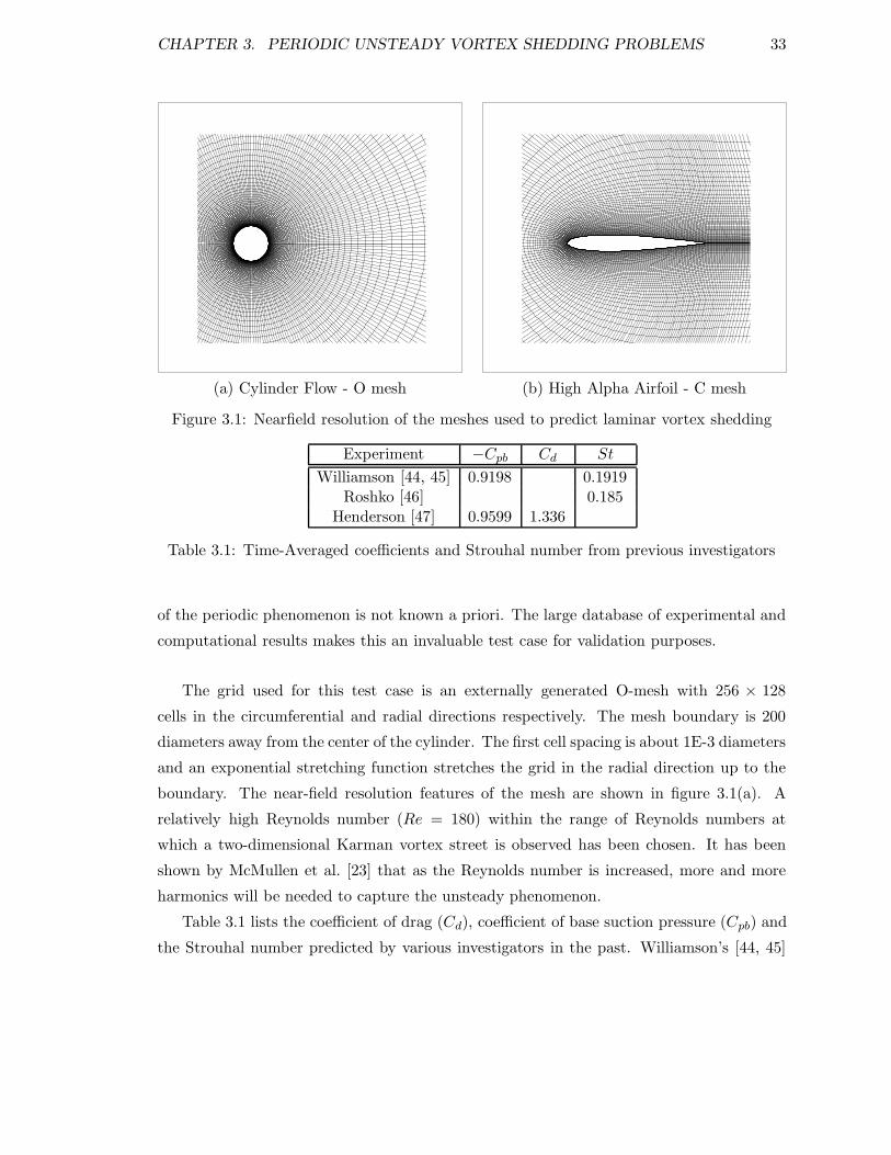
CHAPTER 3. PERIODIC UNSTEADY VORTEX SHEDDING PROBLEMS 33
(a) Cylinder Flow - O mesh (b) High Alpha Airfoil - C mesh
Figure 3.1: Nearfield resolution of the meshes used to predict laminar vortex shedding
Experiment −Cpb Cd St
Williamson [44, 45] 0.9198 0.1919Roshko [46] 0.185
Henderson [47] 0.9599 1.336
Table 3.1: Time-Averaged coefficients and Strouhal number from previous investigators
of the periodic phenomenon is not known a priori. The large database of experimental and
computational results makes this an invaluable test case for validation purposes.
The grid used for this test case is an externally generated O-mesh with 256 × 128
cells in the circumferential and radial directions respectively. The mesh boundary is 200
diameters away from the center of the cylinder. The first cell spacing is about 1E-3 diameters
and an exponential stretching function stretches the grid in the radial direction up to the
boundary. The near-field resolution features of the mesh are shown in figure 3.1(a). A
relatively high Reynolds number (Re = 180) within the range of Reynolds numbers at
which a two-dimensional Karman vortex street is observed has been chosen. It has been
shown by McMullen et al. [23] that as the Reynolds number is increased, more and more
harmonics will be needed to capture the unsteady phenomenon.
Table 3.1 lists the coefficient of drag (Cd), coefficient of base suction pressure (Cpb) and
the Strouhal number predicted by various investigators in the past. Williamson’s [44, 45]
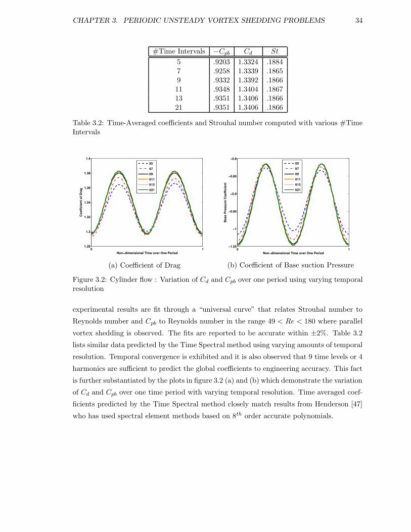
CHAPTER 3. PERIODIC UNSTEADY VORTEX SHEDDING PROBLEMS 34
#Time Intervals −Cpb Cd St
5 .9203 1.3324 .18847 .9258 1.3339 .18659 .9332 1.3392 .186611 .9348 1.3404 .186713 .9351 1.3406 .186621 .9351 1.3406 .1866
Table 3.2: Time-Averaged coefficients and Strouhal number computed with various #TimeIntervals
0 11.28
1.3
1.32
1.34
1.36
1.38
1.4
Non−dimensional Time over One Period
Coef
ficie
nt o
f Dra
g
it5it7it9it11it13it21
(a) Coefficient of Drag
0 1−1.05
−1
−0.95
−0.9
−0.85
−0.8
Non−dimensional Time over One Period
Base
Pre
ssur
e Co
effic
ient
it5it7it9it11it13it21
(b) Coefficient of Base suction Pressure
Figure 3.2: Cylinder flow : Variation of Cd and Cpb over one period using varying temporalresolution
experimental results are fit through a “universal curve” that relates Strouhal number to
Reynolds number and Cpb to Reynolds number in the range 49 < Re < 180 where parallel
vortex shedding is observed. The fits are reported to be accurate within ±2%. Table 3.2
lists similar data predicted by the Time Spectral method using varying amounts of temporal
resolution. Temporal convergence is exhibited and it is also observed that 9 time levels or 4
harmonics are sufficient to predict the global coefficients to engineering accuracy. This fact
is further substantiated by the plots in figure 3.2 (a) and (b) which demonstrate the variation
of Cd and Cpb over one time period with varying temporal resolution. Time averaged coef-
ficients predicted by the Time Spectral method closely match results from Henderson [47]
who has used spectral element methods based on 8th order accurate polynomials.
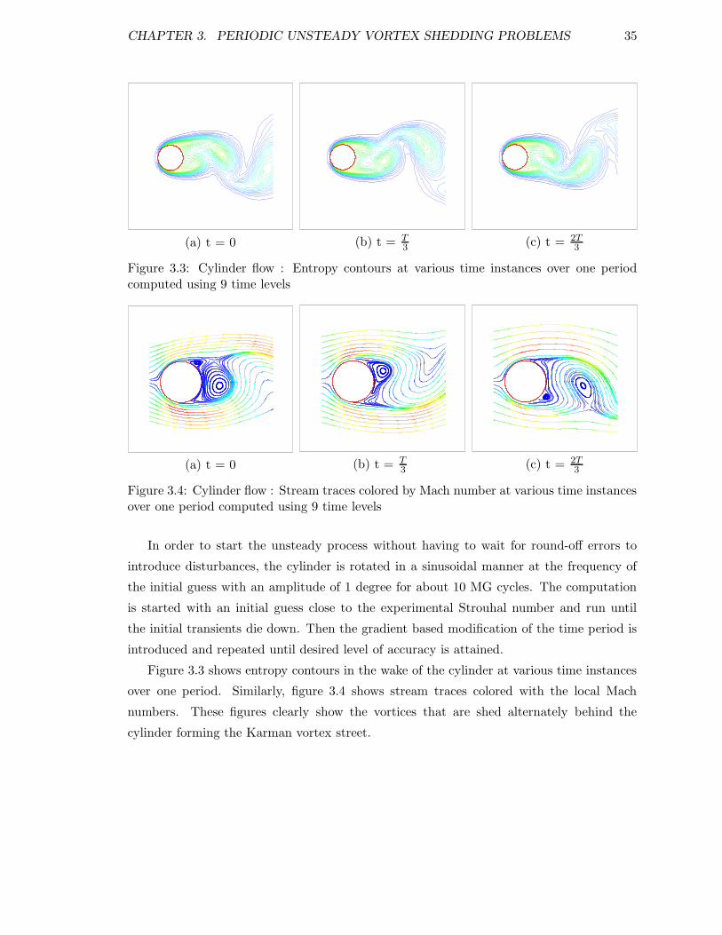
CHAPTER 3. PERIODIC UNSTEADY VORTEX SHEDDING PROBLEMS 35
(a) t = 0 (b) t = T3 (c) t = 2T
3
Figure 3.3: Cylinder flow : Entropy contours at various time instances over one periodcomputed using 9 time levels
(a) t = 0 (b) t = T3 (c) t = 2T
3
Figure 3.4: Cylinder flow : Stream traces colored by Mach number at various time instancesover one period computed using 9 time levels
In order to start the unsteady process without having to wait for round-off errors to
introduce disturbances, the cylinder is rotated in a sinusoidal manner at the frequency of
the initial guess with an amplitude of 1 degree for about 10 MG cycles. The computation
is started with an initial guess close to the experimental Strouhal number and run until
the initial transients die down. Then the gradient based modification of the time period is
introduced and repeated until desired level of accuracy is attained.
Figure 3.3 shows entropy contours in the wake of the cylinder at various time instances
over one period. Similarly, figure 3.4 shows stream traces colored with the local Mach
numbers. These figures clearly show the vortices that are shed alternately behind the
cylinder forming the Karman vortex street.
CHAPTER 3. PERIODIC UNSTEADY VORTEX SHEDDING PROBLEMS 36
3.2.2 High Angle of Attack Airfoil
The viscous flow over a NACA0012 airfoil at Re = 1000 fixed at 20 degrees angle of attack
shows periodic vortex shedding with a large shear layer zone on the suction side of the
airfoil surface. This case poses as an interesting test case for the Time Spectral approach
in combination with computing the time period. The detail of the C-mesh used for this
computation is shown in figure 3.1(b). The mesh consists of 256 × 64 cells and has been
generated using conformal mapping. The first cell spacing of the grid is 1E-4 chords.
Similar to the cylinder case, starting with an initial guess (based on results from previous
investigators [48]), the computation using a fixed time period is carried out until some
residual level. The transition to a limiting shedding cycle is accelerated with a couple of
initial pitches of the airfoil with an amplitude of .5 degrees about a mean of 20 degrees.
Then, the gradient based alteration of the time period is introduced to achieve a desired
level of accuracy both for the unsteady solution and the estimate of the exact time period
(TP*).
Figure 3.5 shows convergence to the exact time period starting from the initial guess
using various levels of temporal resolution. Note that as the number of time intervals is in-
creased, the converged time period gets closer to TP*, i.e. temporal convergence is achieved.
At least 9 time levels are required to predict TP* to engineering accuracy. Figure 3.6 shows
the error in the computed time period using varying numbers of time intervals per period,
compared to TP* computed with N = 21. It proves that close to exponential convergence
has been achieved which is evidenced from the linear variation of the error on a semi-log
plot.
The observation that N = 9 (equivalent to 4 harmonics) is all that is required to achieve
engineering accuracy is further affirmed by the plots showing variation of Coefficient of Drag
(figure 3.7(a)) and Coefficient of Lift (figure 3.7(b)) over one period computed using varying
N .
Another set of results was assimilated based on different starting guesses for the time
period. All of them were simulated with N = 9 and figure 3.8 shows their convergence to
the same time period using the gradient based approach. The percentages listed are the
differences in percentage between the exact time period and the initial guess. This trend
eliminates any random results that can occur with a single initial guess computation.
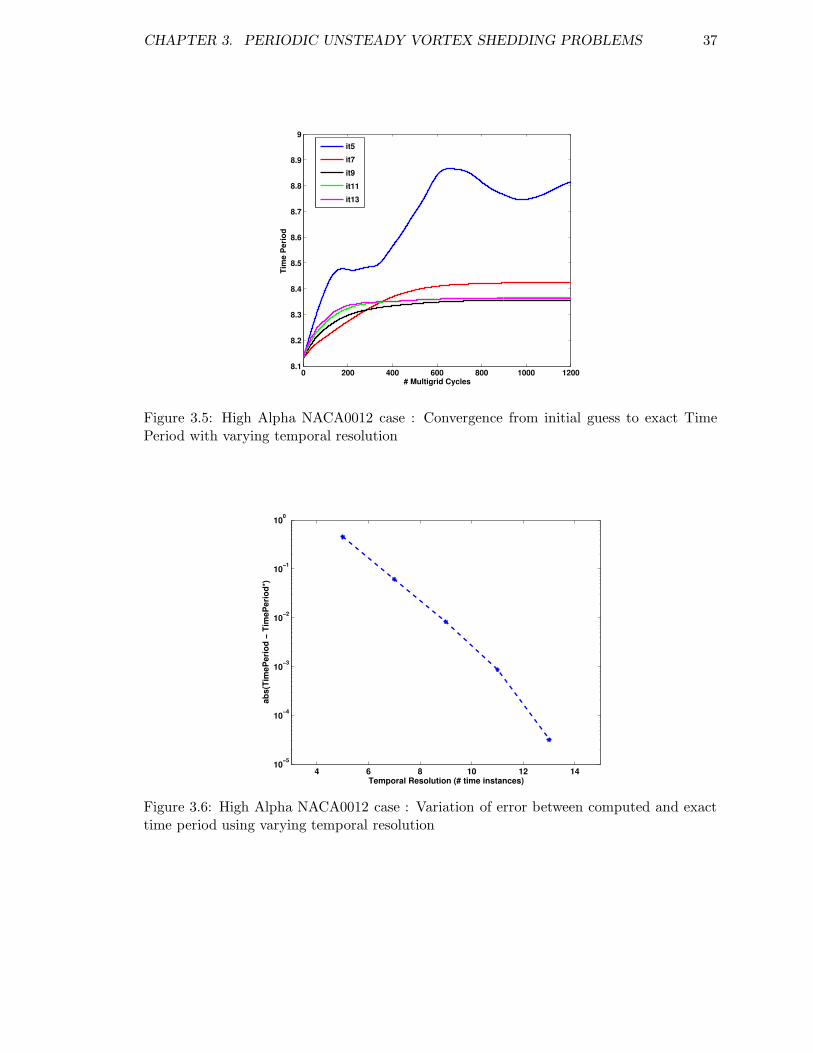
CHAPTER 3. PERIODIC UNSTEADY VORTEX SHEDDING PROBLEMS 37
0 200 400 600 800 1000 12008.1
8.2
8.3
8.4
8.5
8.6
8.7
8.8
8.9
9
# Multigrid Cycles
Tim
e Pe
riod
it5it7it9it11it13
Figure 3.5: High Alpha NACA0012 case : Convergence from initial guess to exact TimePeriod with varying temporal resolution
4 6 8 10 12 1410−5
10−4
10−3
10−2
10−1
100
Temporal Resolution (# time instances)
abs(
Tim
ePer
iod
− Ti
meP
erio
d*)
Figure 3.6: High Alpha NACA0012 case : Variation of error between computed and exacttime period using varying temporal resolution
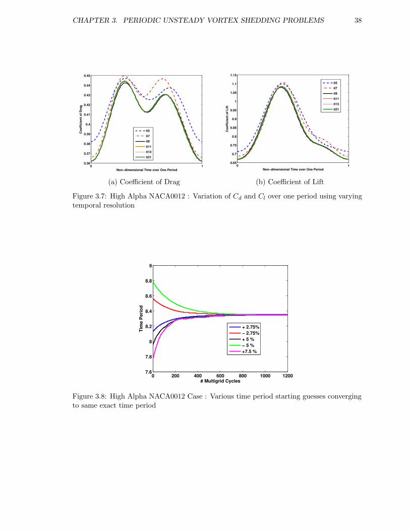
CHAPTER 3. PERIODIC UNSTEADY VORTEX SHEDDING PROBLEMS 38
0 10.36
0.37
0.38
0.39
0.4
0.41
0.42
0.43
0.44
0.45
Non−dimensional Time over One Period
Coef
ficie
nt o
f Dra
g
it5it7it9it11it13it21
(a) Coefficient of Drag
0 10.65
0.7
0.75
0.8
0.85
0.9
0.95
1
1.05
1.1
1.15
Non−dimensional Time over One Period
Coef
ficie
nt o
f Lift
it5it7it9it11it13it21
(b) Coefficient of Lift
Figure 3.7: High Alpha NACA0012 : Variation of Cd and Cl over one period using varyingtemporal resolution
0 200 400 600 800 1000 12007.6
7.8
8
8.2
8.4
8.6
8.8
9
# Multigrid Cycles
Tim
e Pe
riod
+ 2.75%− 2.75%+ 5 %− 5 %+7.5 %
Figure 3.8: High Alpha NACA0012 Case : Various time period starting guesses convergingto same exact time period
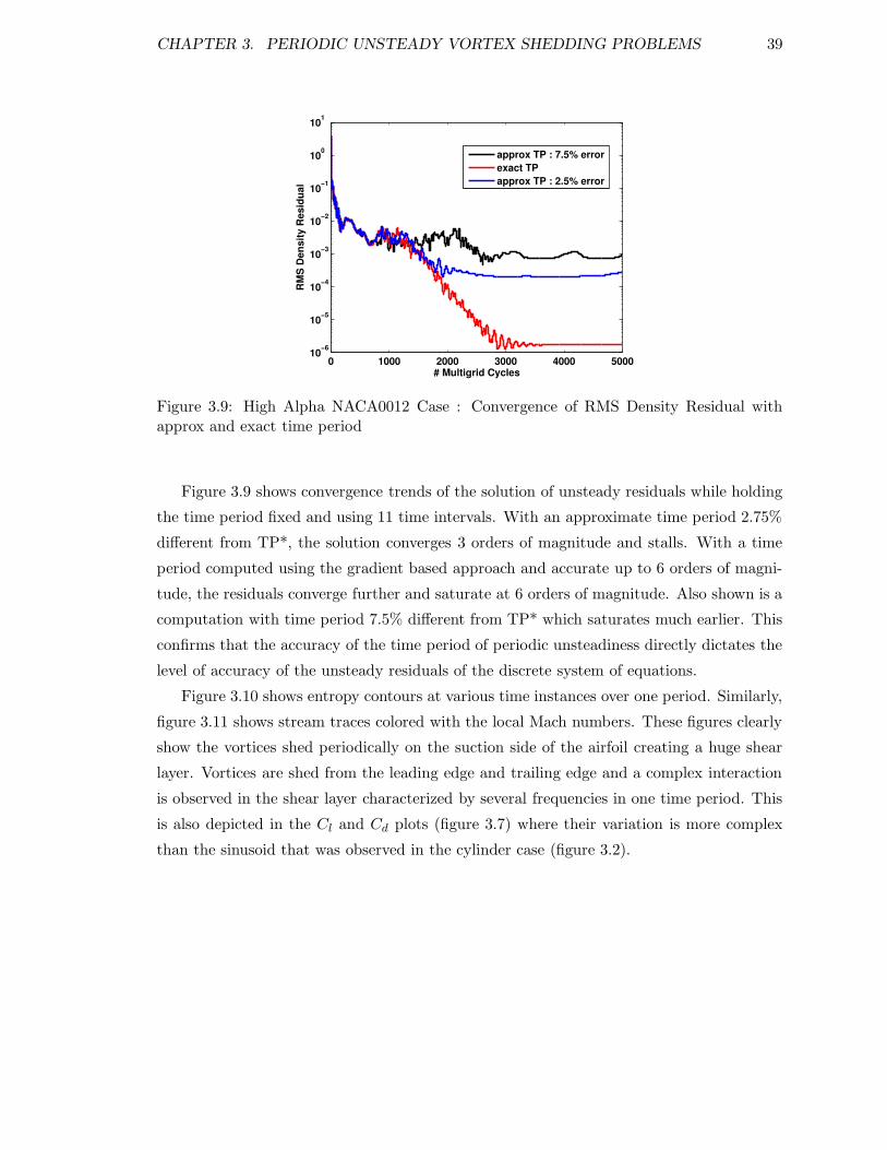
CHAPTER 3. PERIODIC UNSTEADY VORTEX SHEDDING PROBLEMS 39
0 1000 2000 3000 4000 500010−6
10−5
10−4
10−3
10−2
10−1
100
101
# Multigrid Cycles
RMS
Dens
ity R
esid
ual
approx TP : 7.5% errorexact TPapprox TP : 2.5% error
Figure 3.9: High Alpha NACA0012 Case : Convergence of RMS Density Residual withapprox and exact time period
Figure 3.9 shows convergence trends of the solution of unsteady residuals while holding
the time period fixed and using 11 time intervals. With an approximate time period 2.75%
different from TP*, the solution converges 3 orders of magnitude and stalls. With a time
period computed using the gradient based approach and accurate up to 6 orders of magni-
tude, the residuals converge further and saturate at 6 orders of magnitude. Also shown is a
computation with time period 7.5% different from TP* which saturates much earlier. This
confirms that the accuracy of the time period of periodic unsteadiness directly dictates the
level of accuracy of the unsteady residuals of the discrete system of equations.
Figure 3.10 shows entropy contours at various time instances over one period. Similarly,
figure 3.11 shows stream traces colored with the local Mach numbers. These figures clearly
show the vortices shed periodically on the suction side of the airfoil creating a huge shear
layer. Vortices are shed from the leading edge and trailing edge and a complex interaction
is observed in the shear layer characterized by several frequencies in one time period. This
is also depicted in the Cl and Cd plots (figure 3.7) where their variation is more complex
than the sinusoid that was observed in the cylinder case (figure 3.2).
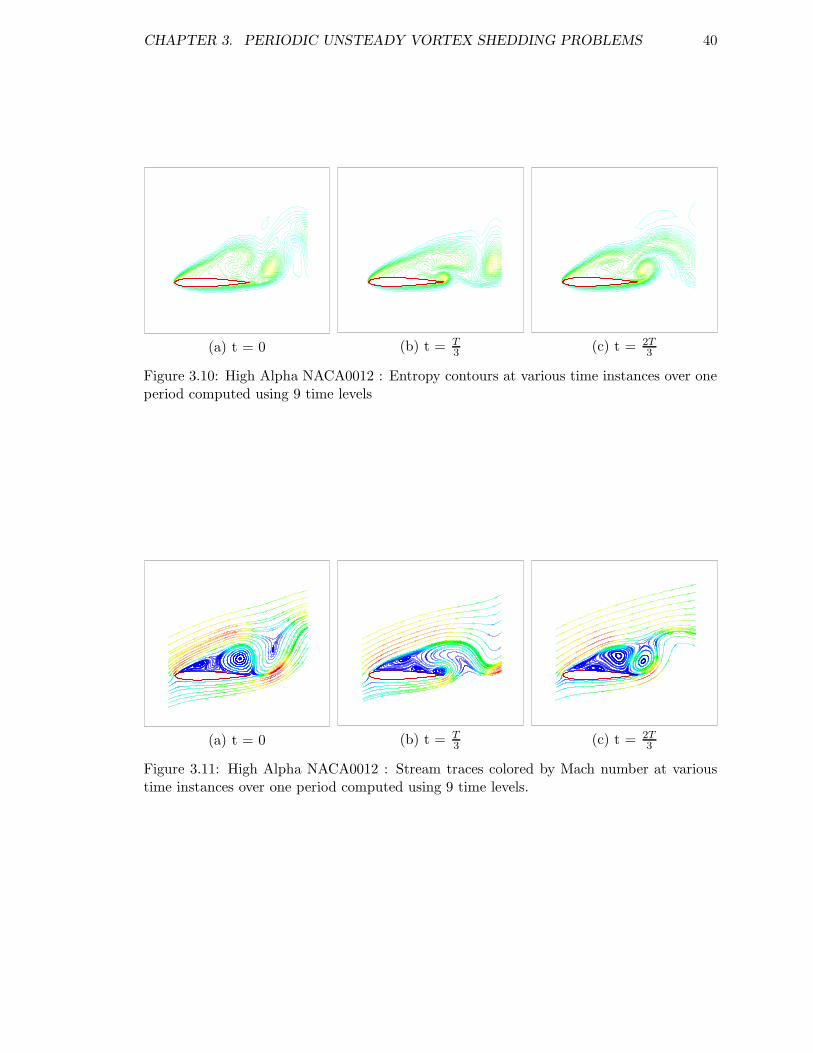
CHAPTER 3. PERIODIC UNSTEADY VORTEX SHEDDING PROBLEMS 40
(a) t = 0 (b) t = T3 (c) t = 2T
3
Figure 3.10: High Alpha NACA0012 : Entropy contours at various time instances over oneperiod computed using 9 time levels
(a) t = 0 (b) t = T3 (c) t = 2T
3
Figure 3.11: High Alpha NACA0012 : Stream traces colored by Mach number at varioustime instances over one period computed using 9 time levels.
Chapter 4
Algorithms for Turbomachinery
Calculations
The first part of this chapter describes how the Time Spectral algorithm illustrated in
Chapter 2 can be used to predict unsteady flows in turbomachinery problems. The flow in
a turbomachine is intrinsically unsteady due to the relative motion of rotors and stators
and the natural flow instabilities present in tip gaps and secondary flows. In addition, it is
periodic mostly with a predetermined frequency: flow features repeat after one revolution
of the annulus. Hence, the Time Spectral algorithm is ideally suited for such an application.
The second part of the chapter presents the reduced-order Harmonic Balance method
which is specifically applicable only for turbomachinery problems. This procedure has
demonstrated to significantly lower the cost of multi-stage simulations by resolving only the
dominant features of the unsteady flow field while utilizing some salient characteristics of
turbomachinery flows.
4.1 Time Spectral method for Periodic Sectors
Recall the expressions for the elements of the time derivative operator in the original form
of the Time Spectral algorithm (equation (2.5) and (2.6)),
doddm =
12(−1)m+1cosec(πm
N) : m 6= 0
0 : m = 0
41
CHAPTER 4. ALGORITHMS FOR TURBOMACHINERY CALCULATIONS 42
devenm =
12(−1)m+1cot(πm
N) : m 6= 0
0 : m = 0
These equations can be directly applied to the computation of flows through turbomachiney
provided the computational domain for such a calculation is the entire annulus. This would
amount to using a time span equal to the time period of revolution of the wheel. A large
number of time instances would be required to resolve a high frequency on such a large
time span. A computational domain consisting of millions/billions of grid points to capture
all the fine details of boundary layers, tip gaps etc., in combination with a large number of
time levels for every computational mesh point could force the calculation to be limited by
the available computing power.
In order to lower the cost of the computation, often only a portion of the domain that
is much smaller than the full annulus, a periodic sector, is solved for. A periodic sector is
arrived at by dividing the blade counts in each blade row of the turbomachine by a common
multiple. For example, the NASA Stage 35 compressor which consists of 36 rotors and 46
stators, can be solved on a computational domain spanning half the annulus (18 rotors and
23 stators) in combination with periodic boundary conditions in the azimuthal direction.
In practical turbomachinery configurations, blade counts are chosen such that periodicity
(other than the whole or half annulus) does not occur, thus avoiding resonance. Hence the
possibility of reduction to a periodic sector would be a rare proposition. In such a case,
often the geometry is rescaled (typically, by altering the blade counts and their chords to
maintain solidity) such that a periodic sector could be feasible. For the same NASA Stage
35 compressor example, a possible scaled geometry would consist of 36 rotors and 48 stators,
so the corresponding periodic sector would comprise 3 rotors and 4 stators. The scaling can
be done in a different way so there are 36 rotors and 36 stators, such that an even further
reduction corresponding to a 1-1 configuration results.
The Time Spectral method can be used in its original form for the periodic sector
domain if the problem is solved in a cylindrical coordinate system. However, the flow solver
used in this work uses a Cartesian formulation of the governing equations so it can be
used universally for other problems and is not limited to turbomachinery. This distinction
between coordinate systems is necessary only for vector quantities which are rotated between
periodic boundaries.
The complete details of the modification of the general Time Spectral formulation to
suit sector periodic problems can be found in van der Weide et al. [49] and is presented in

CHAPTER 4. ALGORITHMS FOR TURBOMACHINERY CALCULATIONS 43
Appendix C. The time derivative term for a vector quantity takes the form,
DtU∗
l =2π
TN
N−1∑
n=1
dNn U∗
l+n +2π
TNeNU∗
l . (4.1)
where,
dNn =
1
P
P−1∑
p=0
dMn+pNRp
eN =1
P
P−1∑
p=1
dMpNRp
(4.2)
dMm =
1
2(−1)m+1 cot
(πm
M
)
M is even
1
2(−1)m+1 cosec
(πm
M
)
M is odd
. (4.3)
N is the number of time levels used to discretize the time span covered by the periodic
sector, and P the number of these periodic sectors required to complete the annulus, so that
M = PN . R is the rotation matrix between consecutive sectors and Rp = R×R× · · · ×R.
This modification has brought about a number of notable features to the new time
derivative operator. Firstly, it is no longer a true central difference operator. This is evident
from the definition of dNn in equation (4.2), dN
n 6= dNN−n. Secondly, the time derivative at
point l depends on the state at point l via eN . This was not the case in the original
formulation where the element in the matrix that related the time derivative and the state
at the same instance, dll was always zero. (Note: eN = 0 for scalars) Finally, due to
the presence of the rotation matrix R, the time derivative of every component of a vector
depends on the state of all components.
Recall that in Chapter 2, both even and odd N formulations were presented. The
benefit of one formulation vs. the other was not obvious in the cases that have already
been discussed. But in the case of turbomachinery, especially where the unsteady term
dominates the equation, the distinction between the formulations is crucial. As explained
before, the even N case has one extra zero eigenvalue, thus permitting odd-even modes.
This induces an instability produced by odd-even decoupling between the time levels. The
odd formulation is devoid of this problem and henceforth an odd number of time levels will
be used for the Time Spectral method applied to turbomachinery problems.
Periodic boundary conditions are applied on the lower and upper azimuthal boundaries
CHAPTER 4. ALGORITHMS FOR TURBOMACHINERY CALCULATIONS 44
of the periodic sector. Along the sliding mesh interfaces, information has to be exchanged
between blade rows. Interpolation is done in the spatial direction so that the position of the
receiver’s cell is located in the donor’s computational domain. This could require that the
donor’s information be computed using periodic boundary conditions since a donor need
not physically exist in the adjoining passage due to relatively moving grids.
4.1.1 Results: Scaled NASA Stage 35 Compressor
The flow solver used in this work is SUmb (Stanford University multi-block), a compress-
ible multi-block URANS code developed at Stanford University during the Department of
Energy’s (DoE) ASC [50] (Advanced Simulation and Computing) program. This code su-
persedes an earlier code, TFLO [6, 7, 8], also developed under ASC. TFLO was created by
combining the FLO107MB [51] and Turbo 90 [52, 53] solvers. SUmb uses a cell-centered
finite volume formulation and a variety of central difference and upwind schemes. In this
work, the inviscid fluxes are computed using a central difference scheme augmented with
a standard scalar formulation for the artificial dissipation [33]. The viscous fluxes are
computed using a central discretization. The convergence is accelerated using a standard
geometric multigrid algorithm in combination with an explicit multi-stage Runge-Kutta
scheme. Several different turbulence models are available in SUmb. Eddy-viscosity is mod-
eled for this test case using the standard k − ω model [54]. The turbulence equations are
solved in a segregated manner from the mean flow using a Diagonally-Dominant Alternating
Direction Implicit (DD-ADI) discretization [55] as the basic iterative method.
The high RPM NASA Stage 35 compressor [56] is a low aspect ratio transonic compressor
consisting of one row of 36 rotors rotating at 17,119 RPM followed by a row of 46 stators.
In order to keep the size of the problem within limits, a scaled geometry is used for the
verification of the Time Spectral method. The stator blade counts are reduced to 36 such
that a 1-1 configuration results. This way the computational grid (figure 4.1) is composed of
a single passage in each blade row (if the true geometry is simulated, a computational grid
spanning half the annulus, 18 rotors and 23 stators, would be required). The BDF method
typically requires large CPU times for high rotation rate turbomachinery cases. This large
cost is lowered by using a rather coarse grid (figure 4.2) which consists of 7 blocks with
a total of 773,184 cells. Only a 2W multigrid cycle is used to accelerate the convergence
due to restrictions imposed by the block dimensions. The spacing normal to the viscous
boundaries is such that a y+ value of O(1) is obtained.
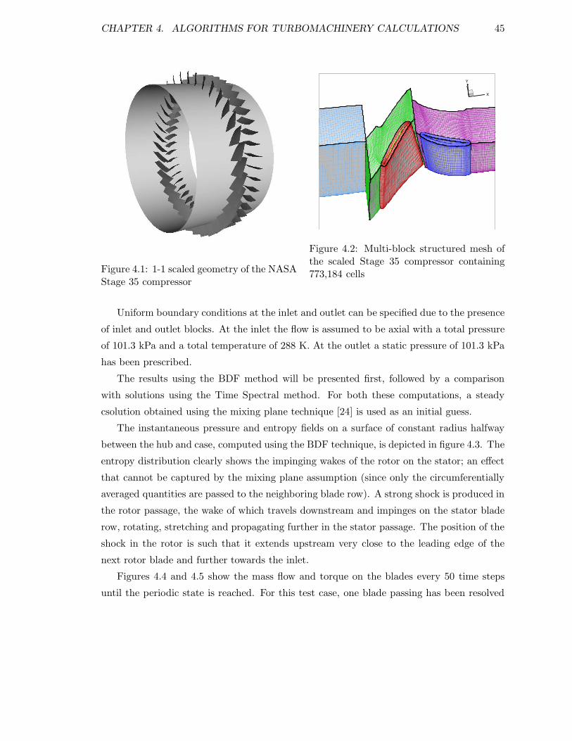
CHAPTER 4. ALGORITHMS FOR TURBOMACHINERY CALCULATIONS 45
Figure 4.1: 1-1 scaled geometry of the NASAStage 35 compressor
X
YZ
Figure 4.2: Multi-block structured mesh ofthe scaled Stage 35 compressor containing773,184 cells
Uniform boundary conditions at the inlet and outlet can be specified due to the presence
of inlet and outlet blocks. At the inlet the flow is assumed to be axial with a total pressure
of 101.3 kPa and a total temperature of 288 K. At the outlet a static pressure of 101.3 kPa
has been prescribed.
The results using the BDF method will be presented first, followed by a comparison
with solutions using the Time Spectral method. For both these computations, a steady
csolution obtained using the mixing plane technique [24] is used as an initial guess.
The instantaneous pressure and entropy fields on a surface of constant radius halfway
between the hub and case, computed using the BDF technique, is depicted in figure 4.3. The
entropy distribution clearly shows the impinging wakes of the rotor on the stator; an effect
that cannot be captured by the mixing plane assumption (since only the circumferentially
averaged quantities are passed to the neighboring blade row). A strong shock is produced in
the rotor passage, the wake of which travels downstream and impinges on the stator blade
row, rotating, stretching and propagating further in the stator passage. The position of the
shock in the rotor is such that it extends upstream very close to the leading edge of the
next rotor blade and further towards the inlet.
Figures 4.4 and 4.5 show the mass flow and torque on the blades every 50 time steps
until the periodic state is reached. For this test case, one blade passing has been resolved
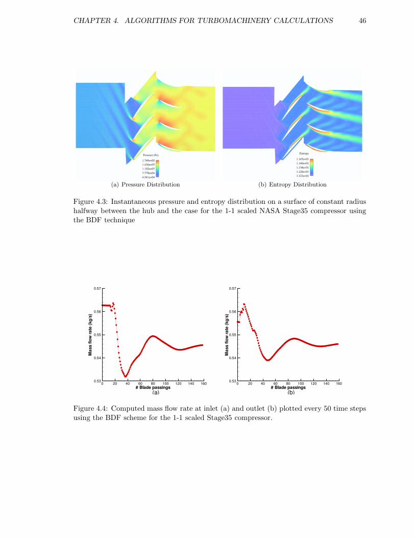
CHAPTER 4. ALGORITHMS FOR TURBOMACHINERY CALCULATIONS 46
(a) Pressure Distribution (b) Entropy Distribution
Figure 4.3: Instantaneous pressure and entropy distribution on a surface of constant radiushalfway between the hub and the case for the 1-1 scaled NASA Stage35 compressor usingthe BDF technique
# Blade passings
Mas
sflo
wra
te(k
g/s)
0 20 40 60 80 100 120 140 1600.53
0.54
0.55
0.56
0.57
(a)# Blade passings
Mas
sflo
wra
te(k
g/s)
0 20 40 60 80 100 120 140 1600.53
0.54
0.55
0.56
0.57
(b)
Figure 4.4: Computed mass flow rate at inlet (a) and outlet (b) plotted every 50 time stepsusing the BDF scheme for the 1-1 scaled Stage35 compressor.
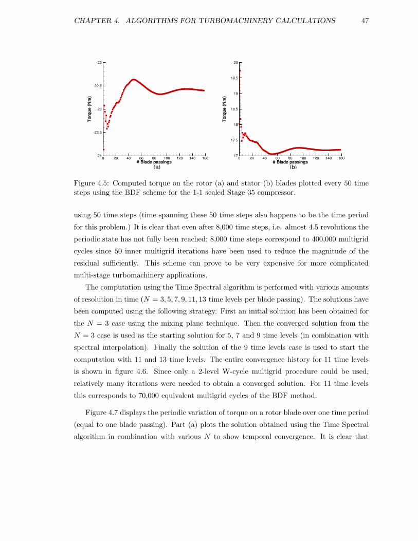
CHAPTER 4. ALGORITHMS FOR TURBOMACHINERY CALCULATIONS 47
# Blade passings
Torq
ue(N
m)
0 20 40 60 80 100 120 140 16017
17.5
18
18.5
19
19.5
20
(b)# Blade passings
Torq
ue(N
m)
0 20 40 60 80 100 120 140 160-24
-23.5
-23
-22.5
-22
(a)
Figure 4.5: Computed torque on the rotor (a) and stator (b) blades plotted every 50 timesteps using the BDF scheme for the 1-1 scaled Stage 35 compressor.
using 50 time steps (time spanning these 50 time steps also happens to be the time period
for this problem.) It is clear that even after 8,000 time steps, i.e. almost 4.5 revolutions the
periodic state has not fully been reached; 8,000 time steps correspond to 400,000 multigrid
cycles since 50 inner multigrid iterations have been used to reduce the magnitude of the
residual sufficiently. This scheme can prove to be very expensive for more complicated
multi-stage turbomachinery applications.
The computation using the Time Spectral algorithm is performed with various amounts
of resolution in time (N = 3, 5, 7, 9, 11, 13 time levels per blade passing). The solutions have
been computed using the following strategy. First an initial solution has been obtained for
the N = 3 case using the mixing plane technique. Then the converged solution from the
N = 3 case is used as the starting solution for 5, 7 and 9 time levels (in combination with
spectral interpolation). Finally the solution of the 9 time levels case is used to start the
computation with 11 and 13 time levels. The entire convergence history for 11 time levels
is shown in figure 4.6. Since only a 2-level W-cycle multigrid procedure could be used,
relatively many iterations were needed to obtain a converged solution. For 11 time levels
this corresponds to 70,000 equivalent multigrid cycles of the BDF method.
Figure 4.7 displays the periodic variation of torque on a rotor blade over one time period
(equal to one blade passing). Part (a) plots the solution obtained using the Time Spectral
algorithm in combination with various N to show temporal convergence. It is clear that
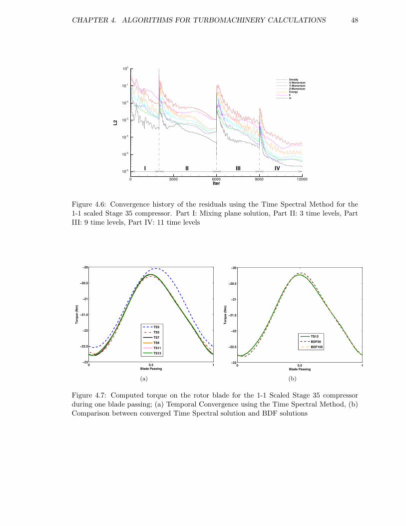
CHAPTER 4. ALGORITHMS FOR TURBOMACHINERY CALCULATIONS 48
Iter
L2
0 3000 6000 9000 12000
10-6
10-5
10-4
10-3
10-2
10-1
100
DensityX-MomentumY-MomentumZ-MomentumEnergykw
IVIIIIII
Figure 4.6: Convergence history of the residuals using the Time Spectral Method for the1-1 scaled Stage 35 compressor. Part I: Mixing plane solution, Part II: 3 time levels, PartIII: 9 time levels, Part IV: 11 time levels
0 0.5 1−23
−22.5
−22
−21.5
−21
−20.5
−20
Blade Passing
Torq
ue (N
m)
TS3TS5TS7TS9TS11TS13
(a)
0 0.5 1−23
−22.5
−22
−21.5
−21
−20.5
−20
Blade Passing
Torq
ue (N
m)
TS13BDF50BDF100
(b)
Figure 4.7: Computed torque on the rotor blade for the 1-1 Scaled Stage 35 compressorduring one blade passing; (a) Temporal Convergence using the Time Spectral Method, (b)Comparison between converged Time Spectral solution and BDF solutions
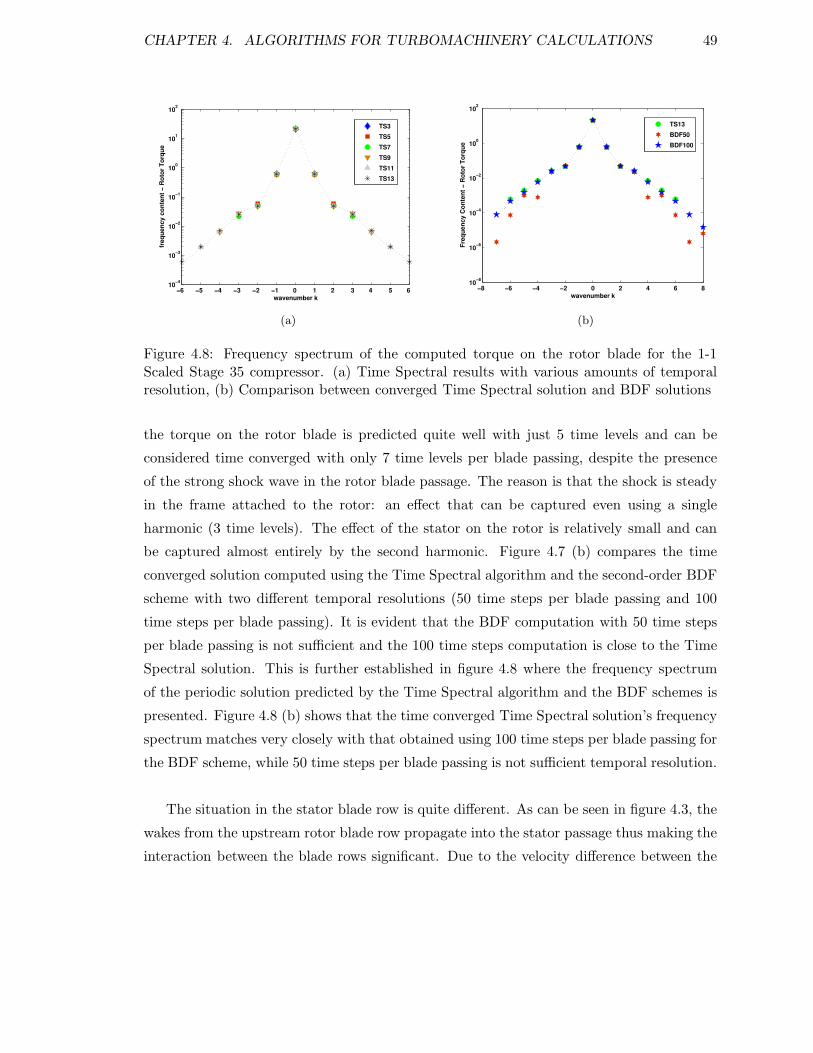
CHAPTER 4. ALGORITHMS FOR TURBOMACHINERY CALCULATIONS 49
−6 −5 −4 −3 −2 −1 0 1 2 3 4 5 6 10−4
10−3
10−2
10−1
100
101
102
wavenumber k
frequ
ency
con
tent
− R
otor
Tor
que
TS3TS5TS7TS9TS11TS13
(a)
−8 −6 −4 −2 0 2 4 6 810−8
10−6
10−4
10−2
100
102
wavenumber k
Freq
uenc
y Co
nten
t − R
otor
Tor
que
TS13BDF50BDF100
(b)
Figure 4.8: Frequency spectrum of the computed torque on the rotor blade for the 1-1Scaled Stage 35 compressor. (a) Time Spectral results with various amounts of temporalresolution, (b) Comparison between converged Time Spectral solution and BDF solutions
the torque on the rotor blade is predicted quite well with just 5 time levels and can be
considered time converged with only 7 time levels per blade passing, despite the presence
of the strong shock wave in the rotor blade passage. The reason is that the shock is steady
in the frame attached to the rotor: an effect that can be captured even using a single
harmonic (3 time levels). The effect of the stator on the rotor is relatively small and can
be captured almost entirely by the second harmonic. Figure 4.7 (b) compares the time
converged solution computed using the Time Spectral algorithm and the second-order BDF
scheme with two different temporal resolutions (50 time steps per blade passing and 100
time steps per blade passing). It is evident that the BDF computation with 50 time steps
per blade passing is not sufficient and the 100 time steps computation is close to the Time
Spectral solution. This is further established in figure 4.8 where the frequency spectrum
of the periodic solution predicted by the Time Spectral algorithm and the BDF schemes is
presented. Figure 4.8 (b) shows that the time converged Time Spectral solution’s frequency
spectrum matches very closely with that obtained using 100 time steps per blade passing for
the BDF scheme, while 50 time steps per blade passing is not sufficient temporal resolution.
The situation in the stator blade row is quite different. As can be seen in figure 4.3, the
wakes from the upstream rotor blade row propagate into the stator passage thus making the
interaction between the blade rows significant. Due to the velocity difference between the
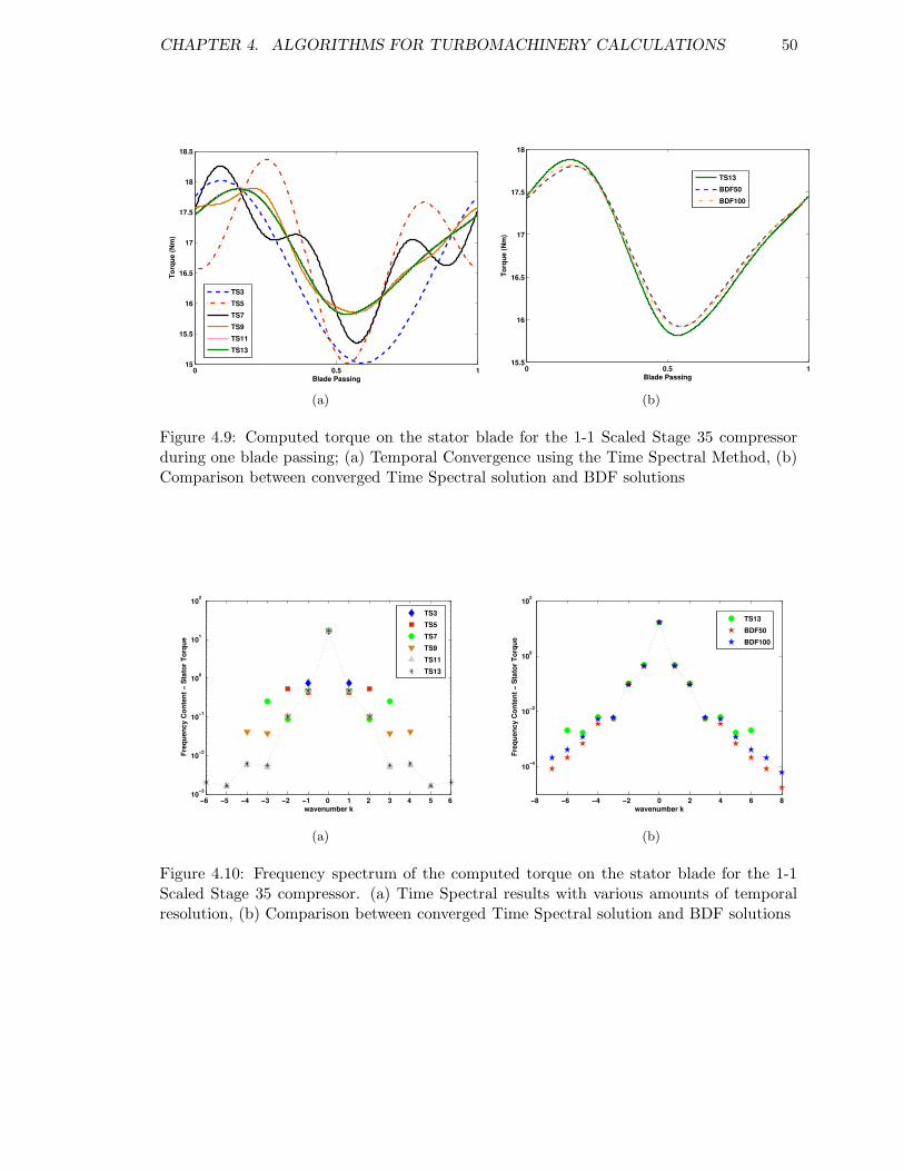
CHAPTER 4. ALGORITHMS FOR TURBOMACHINERY CALCULATIONS 50
0 0.5 115
15.5
16
16.5
17
17.5
18
18.5
Blade Passing
Torq
ue (N
m)
TS3TS5TS7TS9TS11TS13
(a)
0 0.5 115.5
16
16.5
17
17.5
18
Blade Passing
Torq
ue (N
m)
TS13BDF50BDF100
(b)
Figure 4.9: Computed torque on the stator blade for the 1-1 Scaled Stage 35 compressorduring one blade passing; (a) Temporal Convergence using the Time Spectral Method, (b)Comparison between converged Time Spectral solution and BDF solutions
−6 −5 −4 −3 −2 −1 0 1 2 3 4 5 6 10−3
10−2
10−1
100
101
102
wavenumber k
Freq
uenc
y Co
nten
t − S
tato
r Tor
que
TS3TS5TS7TS9TS11TS13
(a)
−8 −6 −4 −2 0 2 4 6 8
10−4
10−2
100
102
wavenumber k
Freq
uenc
y Co
nten
t − S
tato
r Tor
que
TS13BDF50BDF100
(b)
Figure 4.10: Frequency spectrum of the computed torque on the stator blade for the 1-1Scaled Stage 35 compressor. (a) Time Spectral results with various amounts of temporalresolution, (b) Comparison between converged Time Spectral solution and BDF solutions

CHAPTER 4. ALGORITHMS FOR TURBOMACHINERY CALCULATIONS 51
suction and pressure side of the stator blade, indicated by the rotation of the rotor wakes in
the blade passage, higher harmonics are generated. As a result more time levels are needed
to capture these frequencies. Figure 4.9 (a) shows that the solution can be considered time
converged using 11 time levels per blade passing. Part (b) of this figure plots the solution
obtained from the BDF computation using 50 and 100 time steps per blade passing. The
solution using 100 time steps per blade passing is indeed an improvement over the 50
time steps solution, but does not overplot the Time Spectral solution. The reason is more
obvious from figure 4.10 (b) which displays the frequency spectrum of the torque on the
stator computed using the various methods. The Time Spectral solution using 13 time levels
is not able to match the 100 time steps BDF calculation for frequencies with wavenumbers 5
or higher. Apparently, a complex flow field is being simulated which has several frequencies,
although many of them have very low frequency content. Another interesting observation
due to this complex nonlinear flow is exhibited in figure 4.10 (a) which plots the frequency
spectrum of the torque on the stator computed using various N in the Time Spectral
method. N ≤ 9 demonstrate aliasing errors at the end of their frequency spectrum clealy
indicating nonlinear effects. However, these errors have not caused destabilizing effects and
are eliminated by increasing the amount of temporal resolution.
The Time Spectral Method yields computational savings of a factor of 6 in CPU time
compared to the BDF scheme using 50 time steps per blade passing (70,000 vs. 400,000
multigrid cyles) for this case, the 1-1 scaled NASA Stage 35 compressor test case, while
maintaining similar accuracy.
Nevertheless, only an approximate solution to the original problem has been achieved,
since a scaled geometry was used so that the spatial size of the problem was within lim-
its. Even after this reduction in spatial size, if the number of time levels needed by the
Time Spectral method to resolve the unsteady phenomena in question is larger than O(10),
then the savings compared to solving the rescaled problem using the BDF scheme become
marginal, since the cost of the Time Spectral method scales linearly with N . In addition,
the Time Spectral algorithm requires the simultaneous storage of the solution at all N time
instances at every spatial grid point, whereas the second-order BDF scheme only requires
that the solution at the two previous time instances be stored. Such large memory require-
ments could make the Time Spectral algorithm prohibitively expensive, especially when a
high frequency component dominates the flow field.
CHAPTER 4. ALGORITHMS FOR TURBOMACHINERY CALCULATIONS 52
4.2 The Reduced-Order Harmonic Balance Method
The reduced-order Harmonic Balance algorithm for three-dimensional, unsteady, multi-
stage turbomachinery problems will be presented in this section. This time domain algo-
rithm simulates the true geometry of the turbomachine (with the exact blade counts) using
a computational domain consisting of only one blade passage per blade row, thus leading
to drastic savings both in CPU and memory requirements. Modified periodic boundary
conditions are applied on the upper and lower boundaries of the single passage in order
to account for the lack of a common periodic interval for each blade row. The solution
algorithm allows the resolution of a specified set of frequencies in each blade row in order
to obtain the desired computation accuracy; typically, a blade row resolves only the blade
passing frequencies of its neighbors. Since every blade row is setup to resolve different
frequencies the actual Harmonic Balance solution in each of these blade rows is obtained
at different instances in time or time levels. The interaction between blade rows occurs
through sliding mesh interfaces in physical time. Space and time interpolation are carried
out at these interfaces and can, if not properly treated, introduce aliasing errors that can
lead to instabilities. With appropriate resolution of the time interpolation, all instabili-
ties are eliminated. This procedure is shown to significantly reduce the cost of multi-stage
simulations while capturing the dominant unsteady effects.
The following sections address all the above features in detail, and explain the difference
between the Harmonic Balance and the Time Spectral techniques where applicable. Finally
results for both single and multi-stage test cases along with appropriate comparisons with
results from a BDF computation is presented.
4.2.1 Frequencies and Time Derivative Matrix
It is common knowledge in the turbomachinery community that the dominant frequencies
seen by a blade row are those created by the passing of the neighboring blades. For instance,
in an isolated single stage setup with one stator row and one rotor row, the rotor row
perceives the blade passing frequency of the stator row and its higher harmonics, and
the stator row correspondingly resolves the rotor’s blade passing frequency and its higher
harmonics. Hence only a single fundamental and its harmonics need to be resolved in each
blade row. In contrast, a multi-stage case is more complicated. In such cases, each blade
row (except the first and last) is sandwiched between neighboring blade rows and sees blade
CHAPTER 4. ALGORITHMS FOR TURBOMACHINERY CALCULATIONS 53
passing frequencies from all its neighbors. If the blade counts of the neighbors (or their
corresponding pitch) are different, which is the case in most practical turbomachines, these
blade passing frequencies will be different. The solution for the sandwiched blade row should
then resolve various combinations (addition and subtraction of multiples) of the frequencies.
This leads to a situation where there is not one fundamental frequency, but several of them
in addition to their higher harmonics. A set of frequencies to be resolved in each blade
row is specified as an input to the Harmonic Balance algorithm, which can then be used to
predict the unsteady flow through a turbomachine at only a fraction of the cost of the BDF
scheme. This procedure of choosing frequencies is in contrast to the Time Spectral method,
where only one fundamental frequency (corresponding to the rate of rotation of the wheel)
and its higher harmonics are resolved in all the blade rows. This way, all the frequencies
(dominant or otherwise) are resolved, leading to the use of large amounts of resources to
compute information that we are not interested in.
It is well known from the classic paper by Shannon [5] that a minimum of 2K+1 equally
spaced grid points are required to resolve K harmonics of the fundamental frequency. Along
the same lines, in this algorithm a time span is chosen for each blade row that is equal to
the time period of the lowest frequency resolved in that blade row. So if K frequencies
are to be resolved in a blade row, its time span is divided into N = 2K + 1 time levels.
As mentioned before, different frequencies (depending on the blade counts of its neighbors)
could be resolved in each blade row, and hence different time spans and correspondingly
solutions at different physical times could be sought. This is the fundamental difference
between the Harmonic Balance and Time Spectral methods: in the Time Spectral method,
solutions in all blade rows are sought at the same physical times and over the same time
span (equal to the time period of revolution), whereas in the Harmonic Balance method
both the time instances/levels and the time span can differ between blade rows.
The governing equations are solved in a very similar way to that used for the Time Spec-
tral method, where the time derivative term is transformed into a matrix-vector product,
and the equations are marched in pseudo-time to a periodic steady state. The structure
of Dt is explained as follows. Recall the expression for the time derivative matrix in equa-
tion (2.4),
Dt = E−1DE,
derived for the Time Spectral method. The Harmonic Balance method uses the same form
but a different definition of the Fourier matrices E and E−1.
CHAPTER 4. ALGORITHMS FOR TURBOMACHINERY CALCULATIONS 54
As mentioned before, for a periodic problem with time period T , the Time Spectral
method resolves the fundamental frequency, f1 = 2πT
and its higher harmonics fk = kf1. In
such a case, the matrix E can be written as (recall equation (2.3))
Ek,n =1
Ne−ifktn ,
and its inverse E−1 also has anccb analytic expression.
In the Harmonic Balance case, especially in a multistage situation, the frequencies in f
are not integer multiples of each other, and accordingly E−1 has to be computed from E. It
must be noted that it is easier to first construct E−1 analytically (and hence have an analytic
expression for the derivative Dt(E−1)), and then compute E as its inverse. The various
frequencies to be resolved, f, follow the same set of rules specified after equation (2.2). For
real U∗, the number of variables stored could be halved in order to avoid complex arithmetic.
The current complex notation is used for the sake of clarity.
It is evident that once the frequencies are chosen, all other parameters including the
number of time levels, N , the time span over which solution is sought, etc., fall in place.
The frequencies are specified in the following way. The kth frequency resolved in blade row
j is given by,
f rowjk =
nRows∑
i=1
nk,iBi(Ωj − Ωi). (4.4)
Here Bi is the blade count of the ith blade row and Ωi, the rotation rate of the ith blade
row. Ω = 0 for stators. nk,i takes on integer values that are specified as an input by the user
to the solution procedure. Hence K sets of combinations are specified for K frequencies. A
few points can be noted from this equation. Only neighbors contribute to the frequencies
considered by a blade row. A neighbor which is stationary with respect to a blade row does
not contribute to its temporal frequency.
4.2.2 Periodic Boundary Conditions
In the previous section, the problem size was contained by reducing the time span over
which the solution is sought. The Harmonic Balance method uses a computational grid
that spans only one blade passage per blade row instead of the periodic sector that was
required by the Time Spectral method. This procedure of reducing the spatial size of the
problem is explained in this section.
CHAPTER 4. ALGORITHMS FOR TURBOMACHINERY CALCULATIONS 55
Since, in principle, there is no periodic sector anymore, the azimuthal boundaries of a
blade passage no longer satisfy periodic boundary conditions. The boundary conditions are
modified in a manner similar to the phase-lagged condition [25, 27], which states that
U(θ, t) = U(θ + θG, t′), (4.5)
where t′ = t−δt and δt is related to the inter-blade phase angle (the constant phase lead/lag
between adjacent blade passages in the same blade row: typical of blade-row interactions
where the circumferential wavelength of the flow does not coincide with the blade pitch).
In other words, the flow field at an azimuthal distance shifted by the blade gap (θG), can
be generated from the computed flow field at a different time.
Expanding the flow variables in the form of a Fourier series both in time and in the
azimuthal direction, one can write,
U∗(x, r, θ, t) = U(x, r)
N−1∑
n=0
M−1∑
m=0
e−i(ftn+Nθm), (4.6)
where N is the vector of nodal diameters, Nk, an equivalent of the fk in the azimuthal
direction. These are given in terms of the combinations specified for fk and are,
Nk =
nRows∑
i=1
nk,iBi.
The nodal diameters are another way of representing the δt in the phase-lagged condition
(equation (4.5)). Equation (4.6) can be rewritten in terms of the Fourier coefficients U as,
U∗(x, r, θ, t) = U(x, r, θ)
N−1∑
n=0
e−iftn . (4.7)
Comparing equations 4.6 and 4.7,
U(x, r, θ) = U(x, r)
M−1∑
m=0
e−iNθm ,
and hence,
Uk(x, r, θ + θG) = Uk(x, r, θ)e−iNkθG . (4.8)
CHAPTER 4. ALGORITHMS FOR TURBOMACHINERY CALCULATIONS 56
This modified periodic boundary condition is applied to the upper and lower azimuthal
boundaries of a single blade passage and relates the temporal Fourier coefficients at two
azimuthal locations shifted by the blade gap. Since all the computations are done in the
time domain, the expression in equation (4.8) can be written in terms of U∗ as,
U∗(x, r, θ + θG, t) = E−1MEU∗(x, r, θ, t) (4.9)
where M is a diagonal matrix whose elements are
mkk = e−iNkθG .
These equations can be applied directly for scalar quantities, but rotation effects will have
to be taken care of, for the vector quantities. One of the ways to do this would be to apply
equation (4.9) to U∗ which has been transformed to cylindrical coordinates.
The equivalent of these boundary conditions in the Time Spectral algorithm for periodic
sector problems will be periodic boundary conditions where θG (phase difference between
blade passages) will be replaced by the phase difference between consecutive periodic sectors
(θ′G). Also M will be the identity matrix so that E−1ME = I and hence
U∗(x, r, θ + θ′G, t) = U∗(x, r, θ, t),
of course with rotation effects for vector quantities.
4.2.3 Sliding Meshes and Multistage Coupling
This section discusses how information is exchanged across an interface between blade rows
via sliding mesh interfaces and how this transfer is done purely in the time domain. In the
case of the Time Spectral and BDF schemes, the time instances in each blade row at which
the unsteady solution is sought, is exactly the same. If the whole wheel were simulated,
there would always be a donor cell in the adjoining blade row with which information can
be exchanged. When only a periodic fraction of the annulus is solved for, due to relative
motion of the blade rows, it is possible that a physical donor does not exist on the neighbor’s
side and the donor’s information needs to be generated using periodic boundary conditions.
These interpolation procedures, although complicated by the parallel decomposition of the
solver, were relatively straightforward.

CHAPTER 4. ALGORITHMS FOR TURBOMACHINERY CALCULATIONS 57
The situation in the Harmonic Balance method is more complicated. First of all, as in the
Time Spectral case, the flow field in the neighboring blade row must often be generated using
the modified periodic boundary conditions discussed in the previous subsection. Secondly,
as mentioned earlier, different frequencies are resolved in adjoining blade rows, and hence
solutions at different instances in time are sought in adjacent rows, i.e. the nth time instance
in rowi and rowi+1 need not correspond to the same physical time. Consequently the donor’s
information has to be generated at both the spatial location and physical time corresponding
to the receiver’s cell.
In the frequency-domain implementation of the Harmonic Balance method proposed by
Ekici and Hall [31, 21] this coupling was done in the frequency domain. On an interface,
the flow variables U∗ on the donor blade row side are Fourier transformed in time to get U
(inverse of equation (4.7)) at each azimuthal location. Since azimuthal grid lines need not
match across the interface, another Fourier transform is performed in the θ direction to get
U. Assuming radially matched grid lines, these coefficients are transferred to the receiving
blade row after applying non-reflecting boundary conditions [17] to eliminate spurious re-
flections due to frequencies that were not included in the specified frequency set. Using the
basis set of fk and Nk on the receiver’s blade row side, U∗ is computed from the Fourier
coefficients.
In our current algorithm, the coupling between adjoining blade rows is done purely in
the time domain, making it a pseudo-spectral method. This choice is made in order to avoid
the storage of Fourier coefficients and to re-use the interpolation machinery already coded
in the SUmb solver. The flow field on the donor side needs to be generated for all the times
corresponding to the receiver side. This is done using trigonometric interpolation in time.
The simplest way to do this is to think in terms of the Fourier coefficients and implement
in the time domain for U∗,
Ureceiver
= Udonor
or
EU∗(treceiver) = EU∗(tdonor),
or
U∗(treceiver) = E−1EU∗(tdonor),
CHAPTER 4. ALGORITHMS FOR TURBOMACHINERY CALCULATIONS 58
where
Ek,n =1
Ne−ifktdonor
n ,
and
Ek,n =1
Ne−ifktreceiver
n .
Note that at these interpolated times, the azimuthal location of the physical donor need
not match with the receiver and hence information has to be generated using the modified
periodic boundary conditions. This situation was discussed in the previous section.
Due to the nonlinear nature of the flow field, higher frequencies that are combinations
of the fundamental frequencies are generated in the flow field. On a grid with N = 2K + 1
time points, only K frequencies can be captured. Higher frequencies and those frequencies
that do not belong to the frequency set alias onto the lower frequencies and corrupt the
information present in the basis set. Once corrupted, there is no way to get rid of these
spurious frequencies. These aliasing errors accumulate as the computation progresses and
can render the entire simulation unstable. This form of instability has been studied in great
detail in the field of spectral methods. One of the conventional ways of dealiasing is by using
Orszag’s “Two-Thirds Rule”[57]. The essence of the method is to capture these spurious
frequencies using a longer stencil (more time points) and then “filter” them out. i.e., in
order to capture K frequencies, instead of using 2K + 1 points, use 3K + 1 points. In this
way the higher frequencies will be captured in the last K wavenumbers, without corrupting
the smaller wavenumbers. The coefficients of the last K Fourier coefficients are then set to
zero (zero padding) before transforming back to physical space.
Solving for N = 3K + 1 time instances in all blade rows and at every spatial grid point
in order to avoid the aliasing problem at the interface, might be unnecessary. Recall that
in Chapter 2, it was shown that even N(= 2K + 2) has an extra zero eigenvalue that could
introduce odd-even decoupling instabilities in the time derivative term. Similarly, using
N = 3K + 1 introduces K extra zero eigenvalues that might not be desirable.
Instead, this algorithm uses more than 2K + 1 time levels only at the sliding mesh
interface for interpolation purposes. This can be accomplished in two ways. Firstly by
keeping the 2K+1 already existing time levels and extending the time span to accommodate
the extra K time levels or secondly by keeping the same time span but increasing the
number of time levels within the time span. The second option is chosen in this work.
Time interpolated data from the donor side is requested not at 2K + 1 time instances
CHAPTER 4. ALGORITHMS FOR TURBOMACHINERY CALCULATIONS 59
(corresponding to the receiver side), but at twice that many instances: one extra time
instance between every two time instances for which the solution is calculated. These half-
way intermediate points are chosen just for ease such that the original time instances can
be used and equally spaced points can be used for the Fourier transform while keeping the
overall time span the same. According to the two-thirds rule, K more time instances would
suffice to capture the higher frequencies.
The spurious higher frequencies can now be captured on these 2(2K + 1) time “grid”
without corrupting the lower wavenumbers. The data on the receiver side now has to be
filtered such that only the 2K + 1 frequencies that belong to the frequency set are used
for the rest of the computation. Zero padding is done by multiplying U∗ with the matrix
E which consists of only the lower frequencies, then inverse transforming back to physical
space to get the filtered data. Hence,
U∗
filtered = E+EU∗
unfiltered, (4.10)
where U ∗
unfiltered is of length 2(2K + 1). Thus E is not square anymore: its size is (2K +
1) × 2(2K + 1), i.e., it is evaluated at 2(2K + 1) time instances but includes only 2K + 1
frequencies fk. Hence E+, the pseudo-inverse of E, replaces E−1 in equation (4.10). Note
that E+E on this extended stencil is not the identity matrix but is equivalent to the zero
padding operation which when multiplied with U ∗
unfiltered results in U ∗
filtered of desired
length 2K + 1.
4.2.4 Results
In this section, computed results using the reduced-order Harmonic Balance method will be
discussed for two test cases. The first is the three-dimensional NASA Stage 35 compressor,
the scaled geometry of which was used for the verification of the Time Spectral method on
periodic sectors. In the present work, the true geometry of the compressor rig will be used
for the application of the Harmonic Balance method. The second test case is Configuration
D, a two-dimensional model of a multi-stage compressor geometry. Inviscid computations
are performed for this test case.
SUmb, the same flow solver used in Section 4.1.1 was used. For the viscous NASA Stage
35 test case, the one-equation Spalart-Allmaras [58] turbulence model was used.
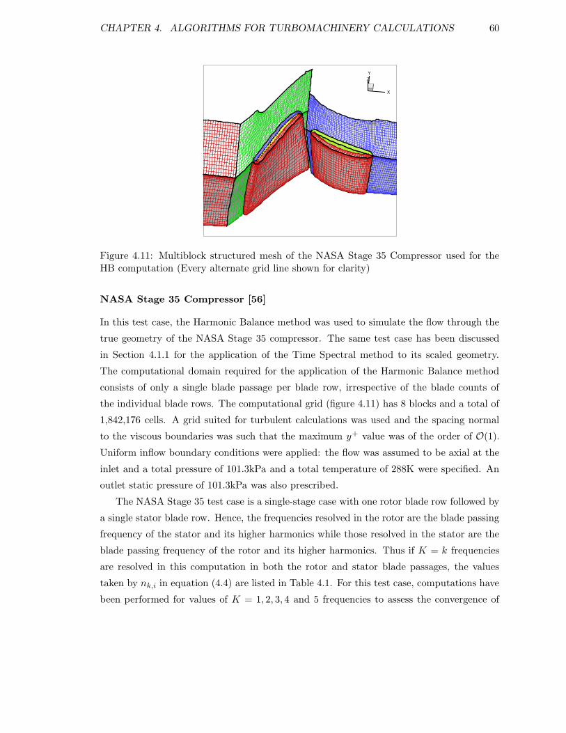
CHAPTER 4. ALGORITHMS FOR TURBOMACHINERY CALCULATIONS 60
X
YZ
Figure 4.11: Multiblock structured mesh of the NASA Stage 35 Compressor used for theHB computation (Every alternate grid line shown for clarity)
NASA Stage 35 Compressor [56]
In this test case, the Harmonic Balance method was used to simulate the flow through the
true geometry of the NASA Stage 35 compressor. The same test case has been discussed
in Section 4.1.1 for the application of the Time Spectral method to its scaled geometry.
The computational domain required for the application of the Harmonic Balance method
consists of only a single blade passage per blade row, irrespective of the blade counts of
the individual blade rows. The computational grid (figure 4.11) has 8 blocks and a total of
1,842,176 cells. A grid suited for turbulent calculations was used and the spacing normal
to the viscous boundaries was such that the maximum y+ value was of the order of O(1).
Uniform inflow boundary conditions were applied: the flow was assumed to be axial at the
inlet and a total pressure of 101.3kPa and a total temperature of 288K were specified. An
outlet static pressure of 101.3kPa was also prescribed.
The NASA Stage 35 test case is a single-stage case with one rotor blade row followed by
a single stator blade row. Hence, the frequencies resolved in the rotor are the blade passing
frequency of the stator and its higher harmonics while those resolved in the stator are the
blade passing frequency of the rotor and its higher harmonics. Thus if K = k frequencies
are resolved in this computation in both the rotor and stator blade passages, the values
taken by nk,i in equation (4.4) are listed in Table 4.1. For this test case, computations have
been performed for values of K = 1, 2, 3, 4 and 5 frequencies to assess the convergence of
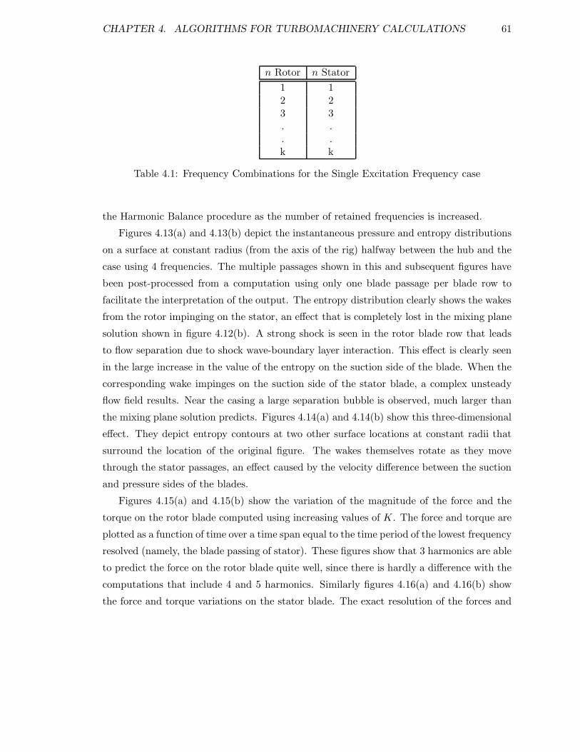
CHAPTER 4. ALGORITHMS FOR TURBOMACHINERY CALCULATIONS 61
n Rotor n Stator
1 12 23 3. .. .k k
Table 4.1: Frequency Combinations for the Single Excitation Frequency case
the Harmonic Balance procedure as the number of retained frequencies is increased.
Figures 4.13(a) and 4.13(b) depict the instantaneous pressure and entropy distributions
on a surface at constant radius (from the axis of the rig) halfway between the hub and the
case using 4 frequencies. The multiple passages shown in this and subsequent figures have
been post-processed from a computation using only one blade passage per blade row to
facilitate the interpretation of the output. The entropy distribution clearly shows the wakes
from the rotor impinging on the stator, an effect that is completely lost in the mixing plane
solution shown in figure 4.12(b). A strong shock is seen in the rotor blade row that leads
to flow separation due to shock wave-boundary layer interaction. This effect is clearly seen
in the large increase in the value of the entropy on the suction side of the blade. When the
corresponding wake impinges on the suction side of the stator blade, a complex unsteady
flow field results. Near the casing a large separation bubble is observed, much larger than
the mixing plane solution predicts. Figures 4.14(a) and 4.14(b) show this three-dimensional
effect. They depict entropy contours at two other surface locations at constant radii that
surround the location of the original figure. The wakes themselves rotate as they move
through the stator passages, an effect caused by the velocity difference between the suction
and pressure sides of the blades.
Figures 4.15(a) and 4.15(b) show the variation of the magnitude of the force and the
torque on the rotor blade computed using increasing values of K. The force and torque are
plotted as a function of time over a time span equal to the time period of the lowest frequency
resolved (namely, the blade passing of stator). These figures show that 3 harmonics are able
to predict the force on the rotor blade quite well, since there is hardly a difference with the
computations that include 4 and 5 harmonics. Similarly figures 4.16(a) and 4.16(b) show
the force and torque variations on the stator blade. The exact resolution of the forces and
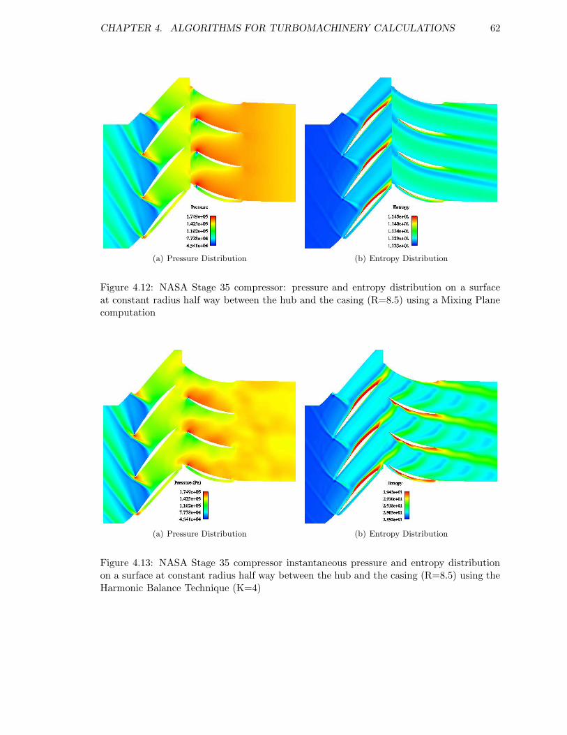
CHAPTER 4. ALGORITHMS FOR TURBOMACHINERY CALCULATIONS 62
(a) Pressure Distribution (b) Entropy Distribution
Figure 4.12: NASA Stage 35 compressor: pressure and entropy distribution on a surfaceat constant radius half way between the hub and the casing (R=8.5) using a Mixing Planecomputation
(a) Pressure Distribution (b) Entropy Distribution
Figure 4.13: NASA Stage 35 compressor instantaneous pressure and entropy distributionon a surface at constant radius half way between the hub and the casing (R=8.5) using theHarmonic Balance Technique (K=4)
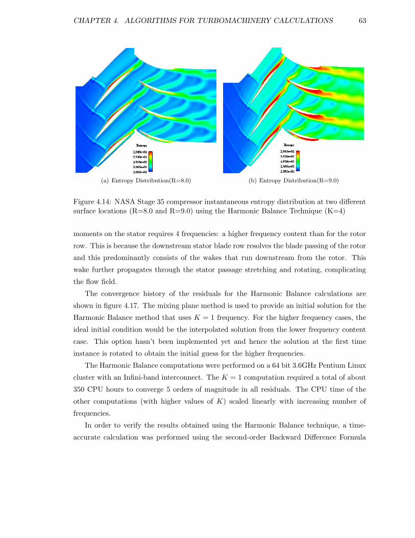
CHAPTER 4. ALGORITHMS FOR TURBOMACHINERY CALCULATIONS 63
(a) Entropy Distribution(R=8.0) (b) Entropy Distribution(R=9.0)
Figure 4.14: NASA Stage 35 compressor instantaneous entropy distribution at two differentsurface locations (R=8.0 and R=9.0) using the Harmonic Balance Technique (K=4)
moments on the stator requires 4 frequencies: a higher frequency content than for the rotor
row. This is because the downstream stator blade row resolves the blade passing of the rotor
and this predominantly consists of the wakes that run downstream from the rotor. This
wake further propagates through the stator passage stretching and rotating, complicating
the flow field.
The convergence history of the residuals for the Harmonic Balance calculations are
shown in figure 4.17. The mixing plane method is used to provide an initial solution for the
Harmonic Balance method that uses K = 1 frequency. For the higher frequency cases, the
ideal initial condition would be the interpolated solution from the lower frequency content
case. This option hasn’t been implemented yet and hence the solution at the first time
instance is rotated to obtain the initial guess for the higher frequencies.
The Harmonic Balance computations were performed on a 64 bit 3.6GHz Pentium Linux
cluster with an Infini-band interconnect. The K = 1 computation required a total of about
350 CPU hours to converge 5 orders of magnitude in all residuals. The CPU time of the
other computations (with higher values of K) scaled linearly with increasing number of
frequencies.
In order to verify the results obtained using the Harmonic Balance technique, a time-
accurate calculation was performed using the second-order Backward Difference Formula
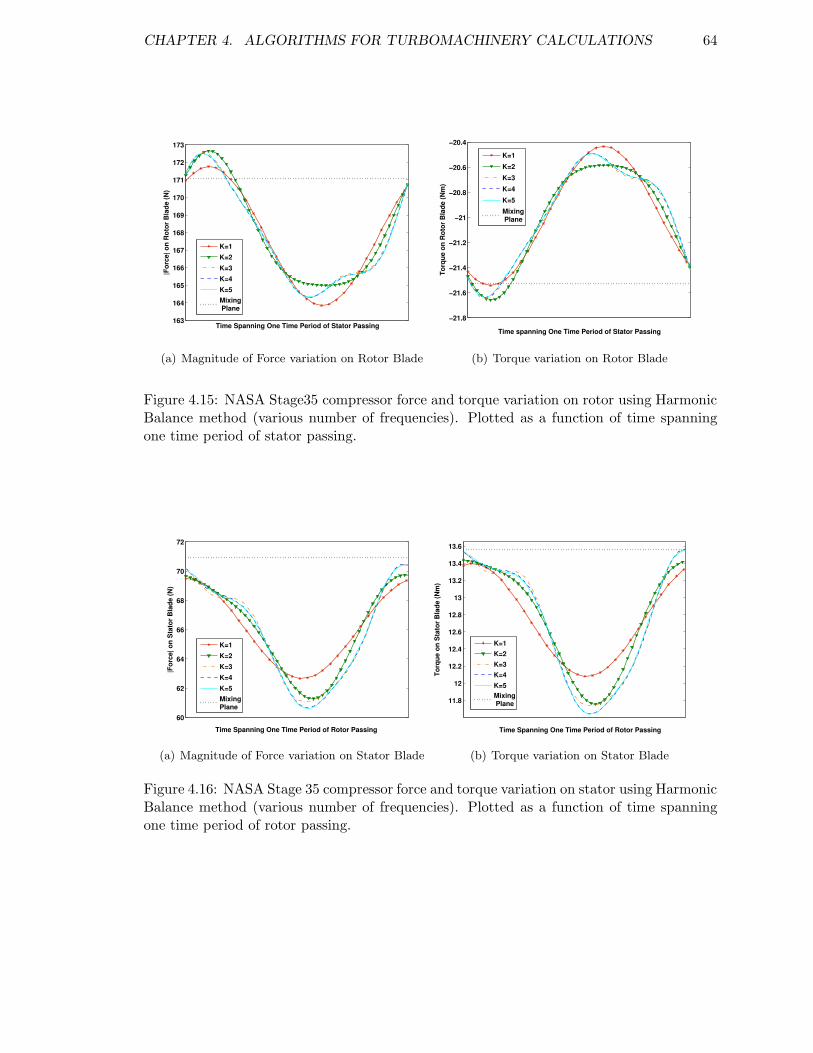
CHAPTER 4. ALGORITHMS FOR TURBOMACHINERY CALCULATIONS 64
163
164
165
166
167
168
169
170
171
172
173
Time Spanning One Time Period of Stator Passing
|For
ce| o
n Ro
tor B
lade
(N)
K=1K=2K=3K=4K=5Mixing Plane
(a) Magnitude of Force variation on Rotor Blade
−21.8
−21.6
−21.4
−21.2
−21
−20.8
−20.6
−20.4
Time spanning One Time Period of Stator Passing
Torq
ue o
n Ro
tor B
lade
(Nm
)
K=1K=2K=3K=4K=5Mixing Plane
(b) Torque variation on Rotor Blade
Figure 4.15: NASA Stage35 compressor force and torque variation on rotor using HarmonicBalance method (various number of frequencies). Plotted as a function of time spanningone time period of stator passing.
60
62
64
66
68
70
72
Time Spanning One Time Period of Rotor Passing
|For
ce| o
n St
ator
Bla
de (N
)
K=1K=2K=3K=4K=5MixingPlane
(a) Magnitude of Force variation on Stator Blade
11.8
12
12.2
12.4
12.6
12.8
13
13.2
13.4
13.6
Time Spanning One Time Period of Rotor Passing
Torq
ue o
n St
ator
Bla
de (N
m)
K=1K=2K=3K=4K=5Mixing Plane
(b) Torque variation on Stator Blade
Figure 4.16: NASA Stage 35 compressor force and torque variation on stator using HarmonicBalance method (various number of frequencies). Plotted as a function of time spanningone time period of rotor passing.
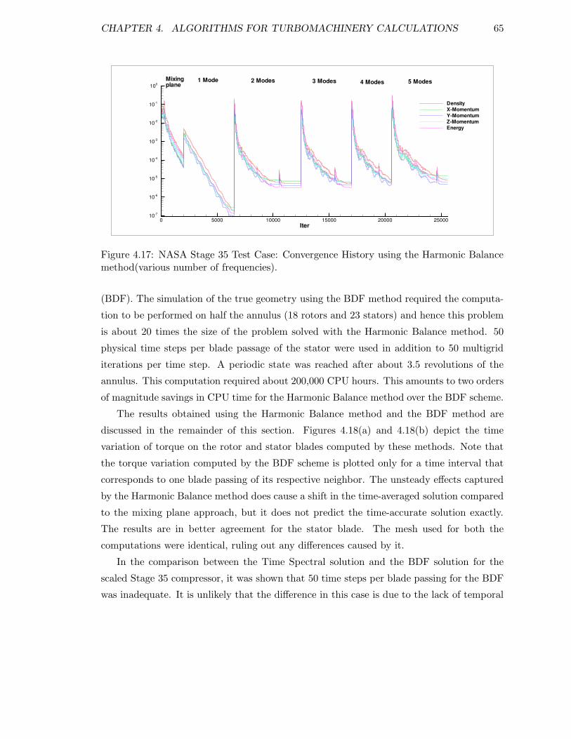
CHAPTER 4. ALGORITHMS FOR TURBOMACHINERY CALCULATIONS 65
Iter0 5000 10000 15000 20000 25000
10-7
10-6
10-5
10-4
10-3
10-2
10-1
100
DensityX-MomentumY-MomentumZ-MomentumEnergy
Mixingplane
1 Mode 2 Modes 3 Modes 4 Modes 5 Modes
Figure 4.17: NASA Stage 35 Test Case: Convergence History using the Harmonic Balancemethod(various number of frequencies).
(BDF). The simulation of the true geometry using the BDF method required the computa-
tion to be performed on half the annulus (18 rotors and 23 stators) and hence this problem
is about 20 times the size of the problem solved with the Harmonic Balance method. 50
physical time steps per blade passage of the stator were used in addition to 50 multigrid
iterations per time step. A periodic state was reached after about 3.5 revolutions of the
annulus. This computation required about 200,000 CPU hours. This amounts to two orders
of magnitude savings in CPU time for the Harmonic Balance method over the BDF scheme.
The results obtained using the Harmonic Balance method and the BDF method are
discussed in the remainder of this section. Figures 4.18(a) and 4.18(b) depict the time
variation of torque on the rotor and stator blades computed by these methods. Note that
the torque variation computed by the BDF scheme is plotted only for a time interval that
corresponds to one blade passing of its respective neighbor. The unsteady effects captured
by the Harmonic Balance method does cause a shift in the time-averaged solution compared
to the mixing plane approach, but it does not predict the time-accurate solution exactly.
The results are in better agreement for the stator blade. The mesh used for both the
computations were identical, ruling out any differences caused by it.
In the comparison between the Time Spectral solution and the BDF solution for the
scaled Stage 35 compressor, it was shown that 50 time steps per blade passing for the BDF
was inadequate. It is unlikely that the difference in this case is due to the lack of temporal
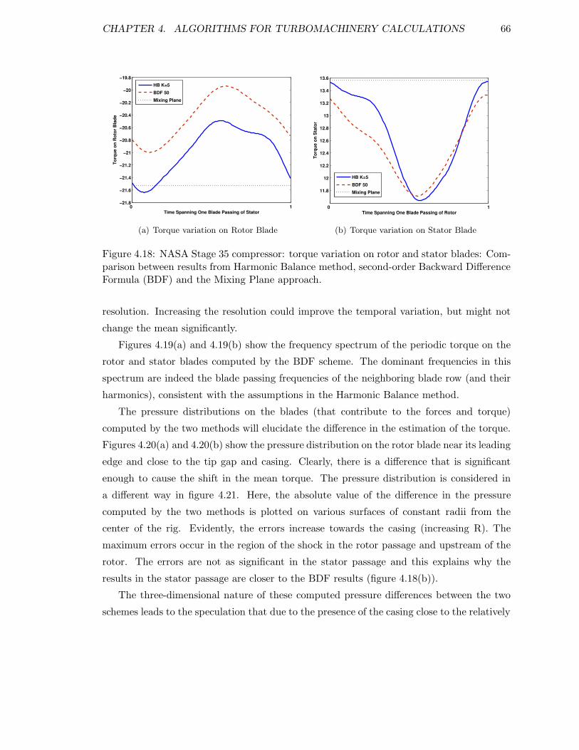
CHAPTER 4. ALGORITHMS FOR TURBOMACHINERY CALCULATIONS 66
0 1−21.8
−21.6
−21.4
−21.2
−21
−20.8
−20.6
−20.4
−20.2
−20
−19.8
Time Spanning One Blade Passing of Stator
Torq
ue o
n Ro
tor B
lade
HB K=5BDF 50Mixing Plane
(a) Torque variation on Rotor Blade
0 1
11.8
12
12.2
12.4
12.6
12.8
13
13.2
13.4
13.6
Time Spanning One Blade Passing of Rotor
Torq
ue o
n St
ator
HB K=5BDF 50Mixing Plane
(b) Torque variation on Stator Blade
Figure 4.18: NASA Stage 35 compressor: torque variation on rotor and stator blades: Com-parison between results from Harmonic Balance method, second-order Backward DifferenceFormula (BDF) and the Mixing Plane approach.
resolution. Increasing the resolution could improve the temporal variation, but might not
change the mean significantly.
Figures 4.19(a) and 4.19(b) show the frequency spectrum of the periodic torque on the
rotor and stator blades computed by the BDF scheme. The dominant frequencies in this
spectrum are indeed the blade passing frequencies of the neighboring blade row (and their
harmonics), consistent with the assumptions in the Harmonic Balance method.
The pressure distributions on the blades (that contribute to the forces and torque)
computed by the two methods will elucidate the difference in the estimation of the torque.
Figures 4.20(a) and 4.20(b) show the pressure distribution on the rotor blade near its leading
edge and close to the tip gap and casing. Clearly, there is a difference that is significant
enough to cause the shift in the mean torque. The pressure distribution is considered in
a different way in figure 4.21. Here, the absolute value of the difference in the pressure
computed by the two methods is plotted on various surfaces of constant radii from the
center of the rig. Evidently, the errors increase towards the casing (increasing R). The
maximum errors occur in the region of the shock in the rotor passage and upstream of the
rotor. The errors are not as significant in the stator passage and this explains why the
results in the stator passage are closer to the BDF results (figure 4.18(b)).
The three-dimensional nature of these computed pressure differences between the two
schemes leads to the speculation that due to the presence of the casing close to the relatively
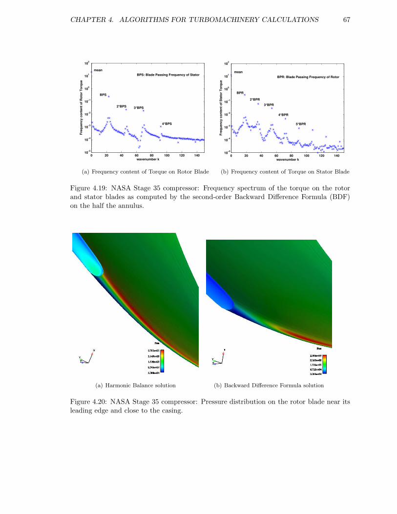
CHAPTER 4. ALGORITHMS FOR TURBOMACHINERY CALCULATIONS 67
0 20 40 60 80 100 120 14010−5
10−4
10−3
10−2
10−1
100
101
102
wavenumber k
Freq
uenc
y co
nten
t of R
otor
Tor
que
mean
2*BPS
BPS
3*BPS
4*BPS
BPS: Blade Passing Frequency of Stator
(a) Frequency content of Torque on Rotor Blade
0 20 40 60 80 100 120 14010−5
10−4
10−3
10−2
10−1
100
101
102
wavenumber k
Freq
uenc
y co
nten
t of S
tato
r Tor
que
mean
3*BPR2*BPR
BPR
4*BPR
5*BPR
BPR: Blade Passing Frequency of Rotor
(b) Frequency content of Torque on Stator Blade
Figure 4.19: NASA Stage 35 compressor: Frequency spectrum of the torque on the rotorand stator blades as computed by the second-order Backward Difference Formula (BDF)on the half the annulus.
(a) Harmonic Balance solution (b) Backward Difference Formula solution
Figure 4.20: NASA Stage 35 compressor: Pressure distribution on the rotor blade near itsleading edge and close to the casing.
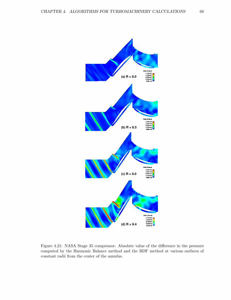
CHAPTER 4. ALGORITHMS FOR TURBOMACHINERY CALCULATIONS 68
(a) R = 8.0
(b) R = 8.5
(c) R = 9.0
(d) R = 9.4
Figure 4.21: NASA Stage 35 compressor: Absolute value of the difference in the pressurecomputed by the Harmonic Balance method and the BDF method at various surfaces ofconstant radii from the center of the annulus.
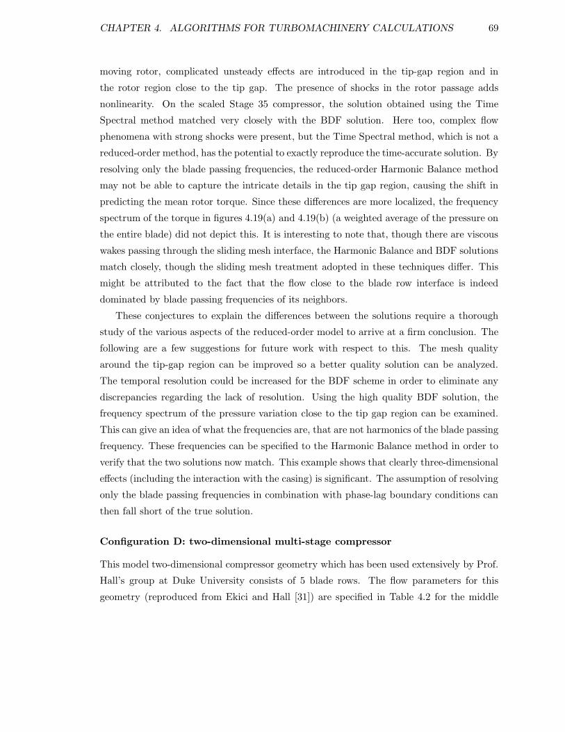
CHAPTER 4. ALGORITHMS FOR TURBOMACHINERY CALCULATIONS 69
moving rotor, complicated unsteady effects are introduced in the tip-gap region and in
the rotor region close to the tip gap. The presence of shocks in the rotor passage adds
nonlinearity. On the scaled Stage 35 compressor, the solution obtained using the Time
Spectral method matched very closely with the BDF solution. Here too, complex flow
phenomena with strong shocks were present, but the Time Spectral method, which is not a
reduced-order method, has the potential to exactly reproduce the time-accurate solution. By
resolving only the blade passing frequencies, the reduced-order Harmonic Balance method
may not be able to capture the intricate details in the tip gap region, causing the shift in
predicting the mean rotor torque. Since these differences are more localized, the frequency
spectrum of the torque in figures 4.19(a) and 4.19(b) (a weighted average of the pressure on
the entire blade) did not depict this. It is interesting to note that, though there are viscous
wakes passing through the sliding mesh interface, the Harmonic Balance and BDF solutions
match closely, though the sliding mesh treatment adopted in these techniques differ. This
might be attributed to the fact that the flow close to the blade row interface is indeed
dominated by blade passing frequencies of its neighbors.
These conjectures to explain the differences between the solutions require a thorough
study of the various aspects of the reduced-order model to arrive at a firm conclusion. The
following are a few suggestions for future work with respect to this. The mesh quality
around the tip-gap region can be improved so a better quality solution can be analyzed.
The temporal resolution could be increased for the BDF scheme in order to eliminate any
discrepancies regarding the lack of resolution. Using the high quality BDF solution, the
frequency spectrum of the pressure variation close to the tip gap region can be examined.
This can give an idea of what the frequencies are, that are not harmonics of the blade passing
frequency. These frequencies can be specified to the Harmonic Balance method in order to
verify that the two solutions now match. This example shows that clearly three-dimensional
effects (including the interaction with the casing) is significant. The assumption of resolving
only the blade passing frequencies in combination with phase-lag boundary conditions can
then fall short of the true solution.
Configuration D: two-dimensional multi-stage compressor
This model two-dimensional compressor geometry which has been used extensively by Prof.
Hall’s group at Duke University consists of 5 blade rows. The flow parameters for this
geometry (reproduced from Ekici and Hall [31]) are specified in Table 4.2 for the middle
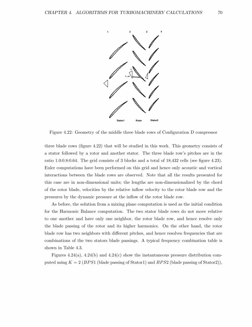
CHAPTER 4. ALGORITHMS FOR TURBOMACHINERY CALCULATIONS 70
1 2 3 4
V
V_rel ROmega
Stator1 Rotor Stator2
Figure 4.22: Geometry of the middle three blade rows of Configuration D compressor
three blade rows (figure 4.22) that will be studied in this work. This geometry consists of
a stator followed by a rotor and another stator. The three blade row’s pitches are in the
ratio 1.0:0.8:0.64. The grid consists of 3 blocks and a total of 18,432 cells (see figure 4.23).
Euler computations have been performed on this grid and hence only acoustic and vortical
interactions between the blade rows are observed. Note that all the results presented for
this case are in non-dimensional units; the lengths are non-dimensionalized by the chord
of the rotor blade, velocities by the relative inflow velocity to the rotor blade row and the
pressures by the dynamic pressure at the inflow of the rotor blade row.
As before, the solution from a mixing plane computation is used as the initial condition
for the Harmonic Balance computation. The two stator blade rows do not move relative
to one another and have only one neighbor, the rotor blade row, and hence resolve only
the blade passing of the rotor and its higher harmonics. On the other hand, the rotor
blade row has two neighbors with different pitches, and hence resolves frequencies that are
combinations of the two stators blade passings. A typical frequency combination table is
shown in Table 4.3.
Figures 4.24(a), 4.24(b) and 4.24(c) show the instantaneous pressure distribution com-
puted using K = 2 (BPS1 (blade passing of Stator1) and BPS2 (blade passing of Stator2)),
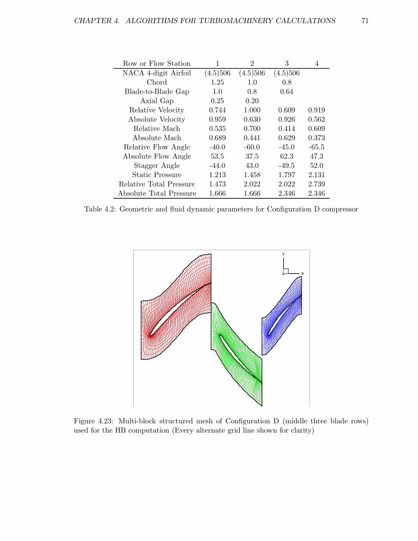
CHAPTER 4. ALGORITHMS FOR TURBOMACHINERY CALCULATIONS 71
Row or Flow Station 1 2 3 4
NACA 4-digit Airfoil (4.5)506 (4.5)506 (4.5)506Chord 1.25 1.0 0.8
Blade-to-Blade Gap 1.0 0.8 0.64Axial Gap 0.25 0.20
Relative Velocity 0.744 1.000 0.609 0.919Absolute Velocity 0.959 0.630 0.926 0.562
Relative Mach 0.535 0.700 0.414 0.609Absolute Mach 0.689 0.441 0.629 0.373
Relative Flow Angle -40.0 -60.0 -45.0 -65.5Absolute Flow Angle 53.5 37.5 62.3 47.3
Stagger Angle -44.0 43.0 -49.5 52.0Static Pressure 1.213 1.458 1.797 2.131
Relative Total Pressure 1.473 2.022 2.022 2.739Absolute Total Pressure 1.666 1.666 2.346 2.346
Table 4.2: Geometric and fluid dynamic parameters for Configuration D compressor
X
Y
Z
Figure 4.23: Multi-block structured mesh of Configuration D (middle three blade rows)used for the HB computation (Every alternate grid line shown for clarity)
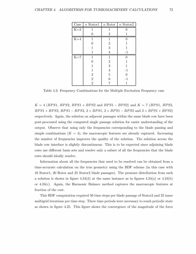
CHAPTER 4. ALGORITHMS FOR TURBOMACHINERY CALCULATIONS 72
Case n Stator1 n Rotor n Stator2
K=2 1 1 00 2 1
K=4 1 1 00 2 11 3 11 4 -1
K=7 1 1 00 2 11 3 11 4 -12 5 02 6 -12 7 1
Table 4.3: Frequency Combinations for the Multiple Excitation Frequency case
K = 4 (BPS1, BPS2, BPS1 + BPS2 and BPS1 − BPS2) and K = 7 (BPS1, BPS2,
BPS1 + BPS2, BPS1 − BPS2, 2 × BPS1, 2 × BPS1 − BPS2 and 2 × BPS1 + BPS2)
respectively. Again, the solution on adjacent passages within the same blade row have been
post-processed using the computed single passage solution for easier understanding of the
output. Observe that using only the frequencies corresponding to the blade passing and
simple combinations (K = 4), the macroscopic features are already captured. Increasing
the number of frequencies improves the quality of the solution. The solution across the
blade row interface is slightly discontinuous. This is to be expected since adjoining blade
rows use different basis sets and resolve only a subset of all the frequencies that the blade
rows should ideally resolve.
Information about all the frequencies that need to be resolved can be obtained from a
time-accurate calculation on the true geometry using the BDF scheme (in this case with
16 Stator1, 20 Rotor and 25 Stator2 blade passages). The pressure distribution from such
a solution is shown in figure 4.24(d) at the same instance as in figures 4.24(a) or 4.24(b)
or 4.24(c). Again, the Harmonic Balance method captures the macroscopic features at
fraction of the cost.
This BDF computation required 50 time steps per blade passage of Stator2 and 25 inner
multigrid iterations per time step. Three time periods were necessary to reach periodic state
as shown in figure 4.25. This figure shows the convergence of the magnitude of the force
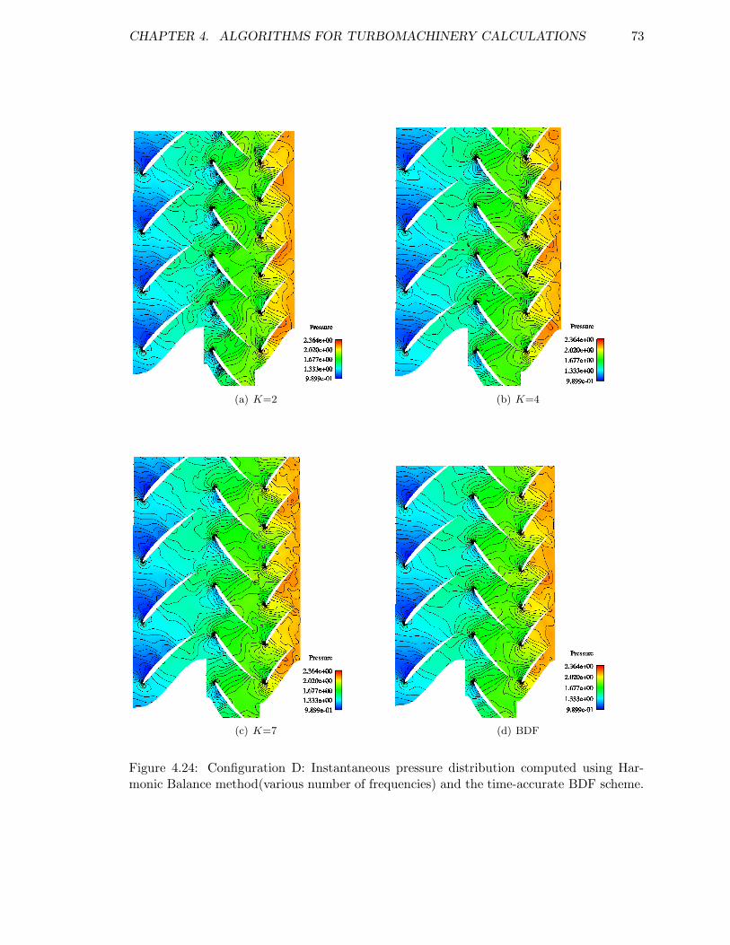
CHAPTER 4. ALGORITHMS FOR TURBOMACHINERY CALCULATIONS 73
(a) K=2 (b) K=4
(c) K=7 (d) BDF
Figure 4.24: Configuration D: Instantaneous pressure distribution computed using Har-monic Balance method(various number of frequencies) and the time-accurate BDF scheme.
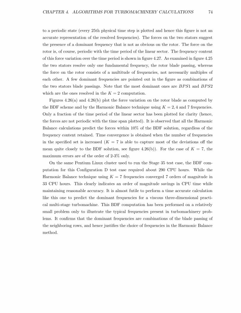
CHAPTER 4. ALGORITHMS FOR TURBOMACHINERY CALCULATIONS 74
to a periodic state (every 25th physical time step is plotted and hence this figure is not an
accurate representation of the resolved frequencies). The forces on the two stators suggest
the presence of a dominant frequency that is not as obvious on the rotor. The force on the
rotor is, of course, periodic with the time period of the linear sector. The frequency content
of this force variation over the time period is shown in figure 4.27. As examined in figure 4.25
the two stators resolve only one fundamental frequency, the rotor blade passing, whereas
the force on the rotor consists of a multitude of frequencies, not necessarily multiples of
each other. A few dominant frequencies are pointed out in the figure as combinations of
the two stators blade passings. Note that the most dominant ones are BPS1 and BPS2
which are the ones resolved in the K = 2 computation.
Figures 4.26(a) and 4.26(b) plot the force variation on the rotor blade as computed by
the BDF scheme and by the Harmonic Balance technique using K = 2, 4 and 7 frequencies.
Only a fraction of the time period of the linear sector has been plotted for clarity (hence,
the forces are not periodic with the time span plotted). It is observed that all the Harmonic
Balance calculations predict the forces within 10% of the BDF solution, regardless of the
frequency content retained. Time convergence is obtained when the number of frequencies
in the specified set is increased (K = 7 is able to capture most of the deviations off the
mean quite closely to the BDF solution, see figure 4.26(b)). For the case of K = 7, the
maximum errors are of the order of 2-3% only.
On the same Pentium Linux cluster used to run the Stage 35 test case, the BDF com-
putation for this Configuration D test case required about 290 CPU hours. While the
Harmonic Balance technique using K = 7 frequencies converged 7 orders of magnitude in
33 CPU hours. This clearly indicates an order of magnitude savings in CPU time while
maintaining reasonable accuracy. It is almost futile to perform a time accurate calculation
like this one to predict the dominant frequencies for a viscous three-dimensional practi-
cal multi-stage turbomachine. This BDF computation has been performed on a relatively
small problem only to illustrate the typical frequencies present in turbomachinery prob-
lems. It confirms that the dominant frequencies are combinations of the blade passing of
the neighboring rows, and hence justifies the choice of frequencies in the Harmonic Balance
method.
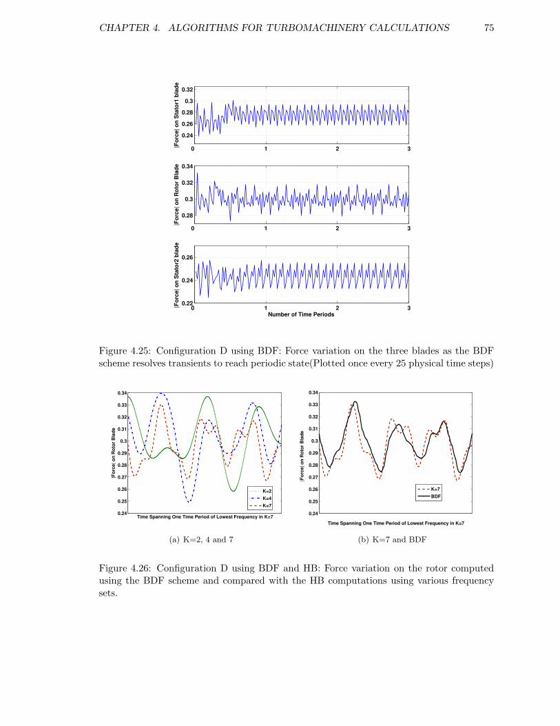
CHAPTER 4. ALGORITHMS FOR TURBOMACHINERY CALCULATIONS 75
0 1 2 3
0.24
0.26
0.28
0.3
0.32
|For
ce| o
n St
ator
1 bl
ade
0 1 2 3
0.28
0.3
0.32
0.34|F
orce
| on
Roto
r Bla
de
0 1 2 30.22
0.24
0.26
Number of Time Periods
|For
ce| o
n St
ator
2 bl
ade
Figure 4.25: Configuration D using BDF: Force variation on the three blades as the BDFscheme resolves transients to reach periodic state(Plotted once every 25 physical time steps)
0.24
0.25
0.26
0.27
0.28
0.29
0.3
0.31
0.32
0.33
0.34
Time Spanning One Time Period of Lowest Frequency in K=7
|For
ce| o
n Ro
tor B
lade
K=2K=4K=7
(a) K=2, 4 and 7
0.24
0.25
0.26
0.27
0.28
0.29
0.3
0.31
0.32
0.33
0.34
Time Spanning One Time Period of Lowest Frequency in K=7
|For
ce| o
n Ro
tor B
lade
K=7BDF
(b) K=7 and BDF
Figure 4.26: Configuration D using BDF and HB: Force variation on the rotor computedusing the BDF scheme and compared with the HB computations using various frequencysets.
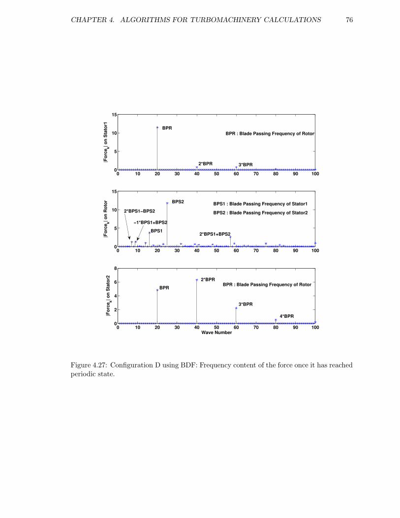
CHAPTER 4. ALGORITHMS FOR TURBOMACHINERY CALCULATIONS 76
0 10 20 30 40 50 60 70 80 90 1000
5
10
15
|For
cek| o
n St
ator
1
0 10 20 30 40 50 60 70 80 90 1000
5
10
15
|For
cek| o
n Ro
tor
0 10 20 30 40 50 60 70 80 90 1000
2
4
6
8
Wave Number
|For
cek| o
n St
ator
2
BPR
2*BPR 3*BPR
2*BPRBPR
3*BPR
4*BPR
−1*BPS1+BPS2
2*BPS1+BPS2BPS1
BPS2
2*BPS1−BPS2
BPR : Blade Passing Frequency of Rotor
BPR : Blade Passing Frequency of Rotor
BPS1 : Blade Passing Frequency of Stator1
BPS2 : Blade Passing Frequency of Stator2
Figure 4.27: Configuration D using BDF: Frequency content of the force once it has reachedperiodic state.
Chapter 5
Conclusions and Future Work
The motivation for this dissertation work stems from the absence of mature, robust and
widely accepted algorithms to solve periodically unsteady problems. This is in contrast to
their steady counterparts which have been studied for decades and have reached a level where
they are used as an everyday design tool. Periodically unsteady problems find themselves
applicable in a plethora of practical fluid mechanics applications and are more recently get-
ting the attention they deserve. Conventionally, they have been treated along the same lines
as unsteady problems (they are!) and hence have been solved in a time-marching fashion.
This essentially meant long integration times and a considerable amount of computational
investment: a perfect recipe to keep engineers/designers at bay!
5.1 Summary: Time Spectral Method
One of the algorithms proposed in this work is the Time Spectral method, an idea that origi-
nates from the Frequency Domain category of algorithms. These algorithms that are specific
to solving periodic unsteady problems use a Fourier-basis in order to take advantage of the
periodicity of the problem. Periodicity is enforced and hence the periodic state is reached
directly surpassing all the numerical transients. As the name suggests, frequency domain
methods have traditionally transformed the equations into frequency space to solve for the
Fourier coefficients, thus decoupling the modes. In contrast, the Time Spectral method
performs all the calculations purely in the time domain, hence requiring minimal modifi-
cations to an already existing steady-state solver. The time derivative term is transformed
into a matrix-vector product and the solution at all time levels simultaneously marched to
77
CHAPTER 5. CONCLUSIONS AND FUTURE WORK 78
periodic state, unlike in a time-marching fashion.
The method was first validated for simple two- and three-dimensional pitching air-
foil/wing test cases where the flow field responded to the single excitation frequency, an
illustration of a forced response problem. It was shown that the Time Spectral method
closely matched the experimental results for integrated quantities and achieved this using
only 4 time levels or 1 harmonic. Evidently, the forcing function was not strong enough to
support higher harmonics due to nonlinearities in the flow.
For the class of problems whose frequency of unsteadiness is not known a priori, like
periodic vortex shedding, the Time Spectral method can be used in combination with a
gradient based approach (similar to McMullen’s GBVTP method [23]) to solve for the
exact time period as part of the solution process. Two two-dimensional laminar vortex
shedding problems were considered to test this concept. One, the well studied Karman
vortex streets behind circular cylinders, for which computational results have been shown
to match experimental data very closely. The other test case is the vortex shedding behind
an airfoil at high angle of attack. For both these test cases, the shedding of vortices has
been captured with small amounts of temporal resolution.
For turbomachinery applications, the algorithm was modified to be applicable for sector
periodic problems in a Cartesian formulation. A RANS calculation was performed on the
1-1 scaled NASA Stage 35 compressor: the Time Spectral method achieved a factor of 6
savings in computational requirements compared to the second-order BDF (time-accurate)
calculation with comparable accuracy. 3 frequencies in the rotor and 5 frequencies in the
stator were required to attain temporal convergence, clearly suggesting nonlinear effects. In
principle, it is possible to apply the Time Spectral method to the true geometry, but then
that would require many more time levels to resolve high frequencies proving to be unfa-
vorable compared to time-accurate methods. This is so firstly because the implementation
is very memory intensive, a consequence of requiring to store the solution at all time levels,
and, secondly because as the time span of the computation increases, the number of time
levels needed to capture the same frequency increases, rendering the matrix-vector product
very expensive.
The Time Spectral method has been applied to other periodic unsteady problems like
the simulation of the flow field around a vertical-axis wind turbines [59], in aeroelastic ap-
plications like the prediction of limit-cycle oscillations [60], for flow fields around helicopter
CHAPTER 5. CONCLUSIONS AND FUTURE WORK 79
rotors in forward flight etc. It is an ideal algorithm that can also be used for predict-
ing flapping-wing related applications. Due to the periodic nature of suction/blowing in
synthetic jets, this algorithm can be suitable for such flow control applications too.
Essentially, the Time Spectral technique is an excellent replacement for time-marching
schemes for periodic unsteady problems characterized by a single excitation frequency and
a narrow frequency spectrum.
5.1.1 Future Directions: Time Spectral Method
The Time Spectral method has the potential for spectral accuracy in time. The true benefits
of this feature can be reaped by combining this with high-order discretizations in space.
Currently an explicit treatment of the time derivative term is considered along with lower
CFL numbers to ensure stability. An implicit treatment might be useful for applications
where the frequency of unsteadiness is high restricting the size of the pseudo-time step.
The gradient-based approach to compute the time period of unsteadiness can be im-
proved by studying alternative optimization strategies, better ways of providing initial
guesses or providing not-so-close guesses.
Currently, temporal convergence is achieved by manually increasing the amount of time
resolution until the solution stops changing. This could be done in an automatic way.
The temporal resolution could also be adaptively changed in the computational domain in
accordance with the amount of nonlinear effects present. In the 1-1 scaled NASA Stage 35
compressor test case computed using the Time Spectral method, it was clearly shown that
the rotor blade row required fewer frequencies than the stator blade row to reach temporal
convergence. In such a situation, it would be desirable to introduce the option of using
different amounts of temporal resolution for the different blade rows. This of course would
be possible only with a different sliding mesh treatment incorporating time interpolation
similar to the one in the Harmonic Balance method.
For large three-dimensional time-periodic problems with a broad range of frequencies, a
low temporal resolution solution obtained using the Time Spectral method, can be provided
as an initial guess for the standard time-accurate scheme. This way the numerical transients
can be bypassed such that a high quality periodic solution can be obtained much faster.
CHAPTER 5. CONCLUSIONS AND FUTURE WORK 80
5.2 Summary: Reduced-Order Harmonic Balance Method
In this work, the Harmonic Balance method proposed by Ekici and Hall [31] has been
adapted so that three-dimensional unsteady Euler and RANS multi-stage turbomachinery
calculations can be performed using a purely time-domain method. This is done while
maintaining accuracy and keeping computational costs low. Similar to the Time Spectral
algorithm, a Fourier representation in time is used such that a periodic state is directly
reached without resolving transients. In addition, the spatial size of the problem is drasti-
cally reduced by using a single passage per blade row for the computational grid irrespective
of the blade counts in each blade row, thus simulating the true geometry. Accuracy is main-
tained by choosing to resolve only the dominant frequencies (which need not be harmonics
of a single excitation frequency) of all blade rows (essentially, combinations of blade pass-
ing frequencies of its neighbors). A set of specified frequencies are resolved in each blade
row and this set can be customized by the analyst/designer based on a trade-off between
accuracy and computational cost. Interaction between blade rows is done via sliding mesh
interfaces where both spatial and spectral time interpolations are performed. Nonlinear
effects in combination with spectral interpolation give rise to aliasing errors which have
been treated properly to ensure the stability of the computation at these interfaces. The
coupling across the sliding mesh interfaces is done purely in the time domain such that an
already existing code can be readily used.
For a simple Euler calculation on a two-dimensional compressor geometry, a cost compar-
ison between the Harmonic Balance method and the time- accurate BDF scheme showed
an order of magnitude savings in CPU requirements. For more complicated test cases
with many more stages and more severe unsteady effects, the Harmonic Balance technique
promises higher savings. A three-dimensional RANS calculation on the true geometry of
the NASA Stage 35 compressor case lead to two orders of magnitude savings for the Har-
monic Balance method in comparison with a BDF solution. Preliminary studies showed
that due to complex three-dimensional effects close to the tip-gap region between the rotor
and the casing, there might be several more frequencies in the flow field. The assumption of
resolving only the blade passing frequencies on the entire domain, in such a situation might
underpredict results.
This reduced-order method can prove to be a valuable tool for a turbomachinery de-
signer, who can now assess a design by customizing the technique so that the most relevant
CHAPTER 5. CONCLUSIONS AND FUTURE WORK 81
flow features can be included in the design process, while achieving this at moderate costs.
5.2.1 Future Directions: Harmonic Balance Method
The three-dimensional single stage compressor test case characterized by a single fundamen-
tal frequency and the two-dimensional one-and-a-half stage compressor test case character-
ized by multiple excitation frequencies established the validity, accuracy and computational
efficiency of the algorithm. Three-dimensional effects on the flow field can be studied fur-
ther to improve the application of phase-lag conditions and the assumption of resolving only
blade passing frequencies.
Applying the method to study the effect of blade passing of a distant neighbor would be
an interesting extension, since a practical turbomachine almost always has many stages and
capturing these effects using a reduced-order model at affordable costs could be worthwhile.
Gust responses and aeroelastic effects whose frequency of unsteadiness is known can be
easily modeled within the Harmonic Balance framework.
The current implementation requires that the same number of frequencies be resolved in
each blade row. In blade rows where the frequency content is small, this procedure may be
unnecessarily expensive. The flexibility of choosing different amounts of temporal resolution
in different blade rows can be added. Currently equally spaced time levels are chosen to
facilitate the use of Fourier series. Other periodic bases supporting unequal spacing between
time instances can be tested such that the relevant frequencies be captured efficiently.
For turbomachines with a higher number of stages, a reduced order model like the one
proposed in this work would not be adequate if a very high fidelity solution is sought,
unless a very large number of frequencies are resolved. Features like tip vortices, whose
shedding frequency cannot be estimated beforehand, and whose frequency is not related to
the rotation rate of the wheel, cannot be predicted by the Harmonic Balance method. In
such a case, a quick calculation can be done where only the immediate neighbor’s blade
passing frequencies are resolved. This solution could then be provided as an initial guess to
a time-accurate method, so that a high quality periodic solution can be obtained bypassing
most of the numerical transients.

Appendix A
Navier-Stokes Equations
The Navier-Stokes equations which describe the behavior of a fluid are derived from basic
principles of conservation of mass, momentum and energy. In its most general form, a
conservation law states that the rate of change of a quantity in a control volume must be
equal to the net volume of the quantity transported through the control volume’s boundaries
plus the amount that is created/destroyed inside the control volume.
In integral form, for an arbitrary volume of fluid Ω in the absence of body forces, the
Navier-Stokes equations read,
∂
∂t
∫
Ω
w dV +
∮
∂Ω
~F · ~N ds = 0.
w is the vector of conserved variables, representing the mass, momentum and energy,
w =
ρ
ρu1
ρu2
ρu3
ρE
.
The second term represents the transport of w across the control volume’s boundary ∂Ω.
~N is the unit normal to the surface pointing outwards. The flux vector ~F is for convenience
82
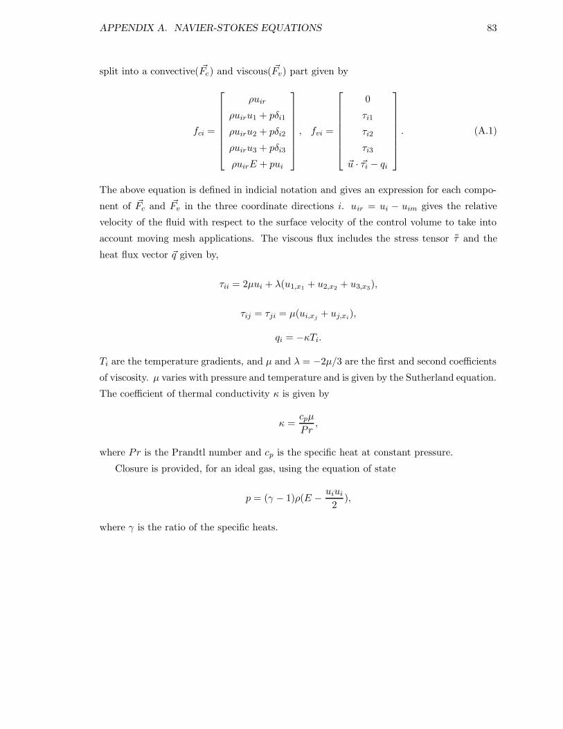
APPENDIX A. NAVIER-STOKES EQUATIONS 83
split into a convective( ~Fc) and viscous( ~Fv) part given by
fci =
ρuir
ρuiru1 + pδi1
ρuiru2 + pδi2
ρuiru3 + pδi3
ρuirE + pui
, fvi =
0
τi1
τi2
τi3
~u · ~τi − qi
. (A.1)
The above equation is defined in indicial notation and gives an expression for each compo-
nent of ~Fc and ~Fv in the three coordinate directions i. uir = ui − uim gives the relative
velocity of the fluid with respect to the surface velocity of the control volume to take into
account moving mesh applications. The viscous flux includes the stress tensor ¯τ and the
heat flux vector ~q given by,
τii = 2µui + λ(u1,x1+ u2,x2
+ u3,x3),
τij = τji = µ(ui,xj+ uj,xi
),
qi = −κTi.
Ti are the temperature gradients, and µ and λ = −2µ/3 are the first and second coefficients
of viscosity. µ varies with pressure and temperature and is given by the Sutherland equation.
The coefficient of thermal conductivity κ is given by
κ =cpµ
Pr,
where Pr is the Prandtl number and cp is the specific heat at constant pressure.
Closure is provided, for an ideal gas, using the equation of state
p = (γ − 1)ρ(E −uiui
2),
where γ is the ratio of the specific heats.
Appendix B
Matrix Operators for Numerical
Differentiation
The numerical differentiation of a discrete periodic function can be expressed as a matrix
operator multiplying a vector consisting of the function values. This is achieved by repre-
senting the function using a Fourier basis. Two formulations can be distinguished depending
on the number of grid points N(odd or even) used to discretize the periodic function U ∗.
The expression for the matrix operator using an even formulation [61, 62, 63] has been
used extensively in computations involving FFTs. The derivation of both the odd and even
formulations will be explained in this section.
Let the function U ∗, periodic on the interval 0 ≤ t ≤ 2π, be discretized using N equally
spaced points tj ,
tj =2πj
Nj = 0, 1, 2, ...N − 1.
B.1 Even Formulation
The discrete Fourier transform of U ∗ is given by
Uk =1
N
N−1∑
j=0
U∗
j e−iktj (B.1)
84
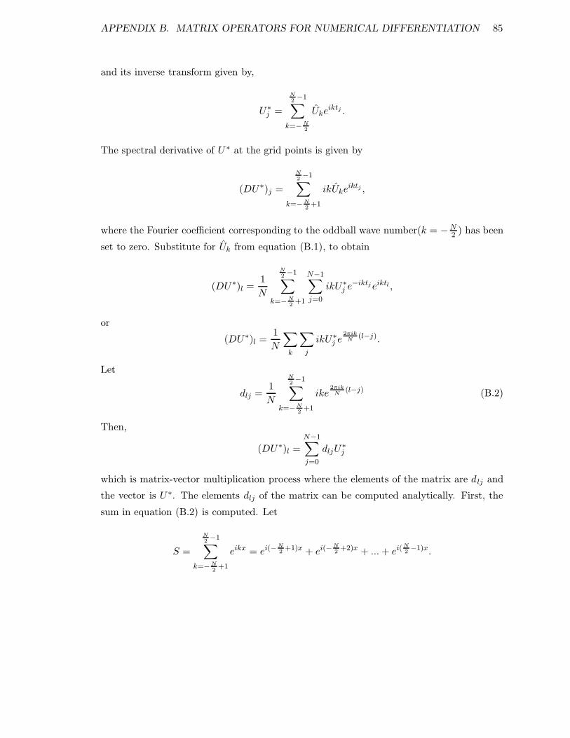
APPENDIX B. MATRIX OPERATORS FOR NUMERICAL DIFFERENTIATION 85
and its inverse transform given by,
U∗
j =
N2−1
∑
k=−N2
Ukeiktj .
The spectral derivative of U ∗ at the grid points is given by
(DU∗)j =
N2−1
∑
k=−N2
+1
ikUkeiktj ,
where the Fourier coefficient corresponding to the oddball wave number(k = −N2 ) has been
set to zero. Substitute for Uk from equation (B.1), to obtain
(DU∗)l =1
N
N2−1
∑
k=−N2
+1
N−1∑
j=0
ikU∗
j e−iktj eiktl ,
or
(DU∗)l =1
N
∑
k
∑
j
ikU∗
j e2πik
N(l−j).
Let
dlj =1
N
N2−1
∑
k=−N2
+1
ike2πik
N(l−j) (B.2)
Then,
(DU∗)l =
N−1∑
j=0
dljU∗
j
which is matrix-vector multiplication process where the elements of the matrix are d lj and
the vector is U ∗. The elements dlj of the matrix can be computed analytically. First, the
sum in equation (B.2) is computed. Let
S =
N2−1
∑
k=−N2
+1
eikx = ei(−N2
+1)x + ei(−N2
+2)x + ... + ei( N2−1)x.
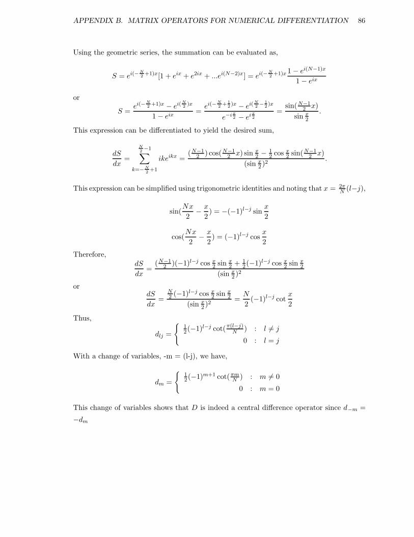
APPENDIX B. MATRIX OPERATORS FOR NUMERICAL DIFFERENTIATION 86
Using the geometric series, the summation can be evaluated as,
S = ei(−N2
+1)x[1 + eix + e2ix + ...ei(N−2)x] = ei(−N2
+1)x 1 − ei(N−1)x
1 − eix
or
S =ei(−N
2+1)x − ei( N
2)x
1 − eix=
ei(−N2
+ 1
2)x − ei( N
2−
1
2)x
e−i x2 − ei x
2
=sin(N−1
2 x)
sin x2
.
This expression can be differentiated to yield the desired sum,
dS
dx=
N2−1
∑
k=−N2
+1
ikeikx =(N−1
2 ) cos(N−12 x) sin x
2 − 12 cos x
2 sin(N−12 x)
(sin x2 )2
.
This expression can be simplified using trigonometric identities and noting that x = 2πN
(l−j),
sin(Nx
2−
x
2) = −(−1)l−j sin
x
2
cos(Nx
2−
x
2) = (−1)l−j cos
x
2
Therefore,dS
dx=
(N−12 )(−1)l−j cos x
2 sin x2 + 1
2 (−1)l−j cos x2 sin x
2
(sin x2 )2
ordS
dx=
N2 (−1)l−j cos x
2 sin x2
(sin x2 )2
=N
2(−1)l−j cot
x
2
Thus,
dlj =
12(−1)l−j cot(π(l−j)
N) : l 6= j
0 : l = j
With a change of variables, -m = (l-j), we have,
dm =
12(−1)m+1 cot(πm
N) : m 6= 0
0 : m = 0
This change of variables shows that D is indeed a central difference operator since d−m =
−dm
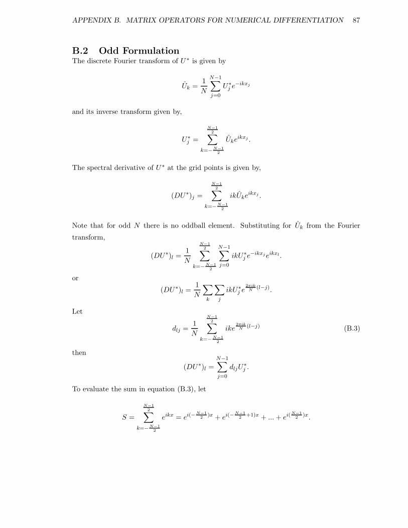
APPENDIX B. MATRIX OPERATORS FOR NUMERICAL DIFFERENTIATION 87
B.2 Odd FormulationThe discrete Fourier transform of U ∗ is given by
Uk =1
N
N−1∑
j=0
U∗
j e−ikxj
and its inverse transform given by,
U∗
j =
N−1
2∑
k=−N−1
2
Ukeikxj .
The spectral derivative of U ∗ at the grid points is given by,
(DU∗)j =
N−1
2∑
k=−N−1
2
ikUkeikxj .
Note that for odd N there is no oddball element. Substituting for Uk from the Fourier
transform,
(DU∗)l =1
N
N−1
2∑
k=−N−1
2
N−1∑
j=0
ikU∗
j e−ikxj eikxl .
or
(DU∗)l =1
N
∑
k
∑
j
ikU∗
j e2πik
N(l−j).
Let
dlj =1
N
N−1
2∑
k=−N−1
2
ike2πik
N(l−j) (B.3)
then
(DU∗)l =
N−1∑
j=0
dljU∗
j .
To evaluate the sum in equation (B.3), let
S =
N−1
2∑
k=−N−1
2
eikx = ei(−N−1
2)x + ei(−N−1
2+1)x + ... + ei( N−1
2)x.
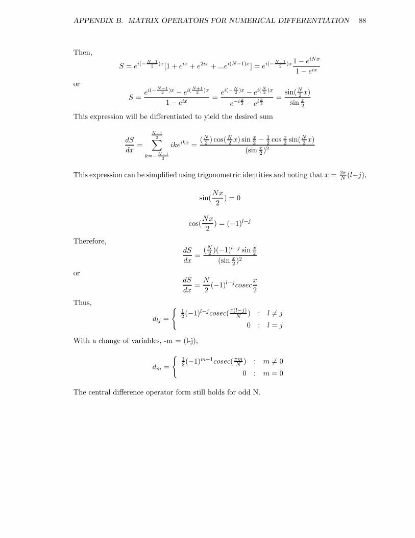
APPENDIX B. MATRIX OPERATORS FOR NUMERICAL DIFFERENTIATION 88
Then,
S = ei(−N−1
2)x[1 + eix + e2ix + ...ei(N−1)x] = ei(−N−1
2)x 1 − eiNx
1 − eix
or
S =ei(−N−1
2)x − ei( N+1
2)x
1 − eix=
ei(−N2
)x − ei( N2
)x
e−i x2 − ei x
2
=sin(N
2 x)
sin x2
This expression will be differentiated to yield the desired sum
dS
dx=
N−1
2∑
k=−N−1
2
ikeikx =(N
2 ) cos(N2 x) sin x
2 − 12 cos x
2 sin(N2 x)
(sin x2 )2
This expression can be simplified using trigonometric identities and noting that x = 2πN
(l−j),
sin(Nx
2) = 0
cos(Nx
2) = (−1)l−j
Therefore,dS
dx=
(N2 )(−1)l−j sin x
2
(sin x2 )2
ordS
dx=
N
2(−1)l−jcosec
x
2
Thus,
dlj =
12(−1)l−jcosec(π(l−j)
N) : l 6= j
0 : l = j
With a change of variables, -m = (l-j),
dm =
12(−1)m+1cosec(πm
N) : m 6= 0
0 : m = 0
The central difference operator form still holds for odd N.
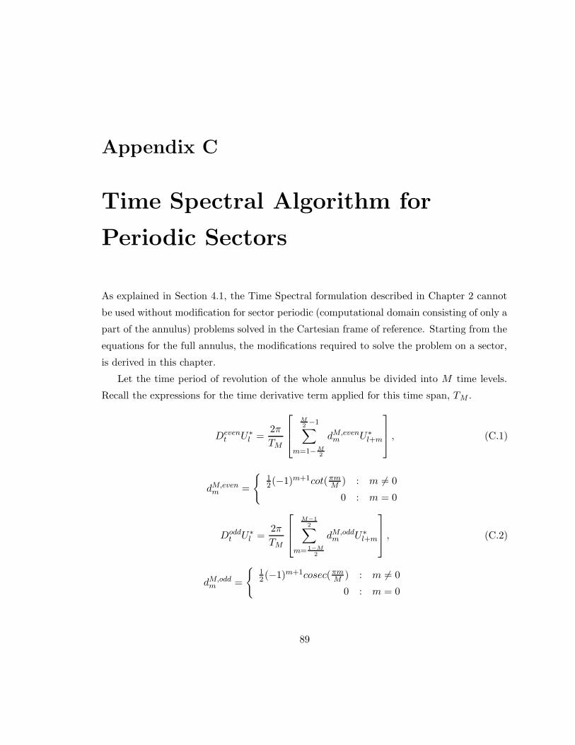
Appendix C
Time Spectral Algorithm for
Periodic Sectors
As explained in Section 4.1, the Time Spectral formulation described in Chapter 2 cannot
be used without modification for sector periodic (computational domain consisting of only a
part of the annulus) problems solved in the Cartesian frame of reference. Starting from the
equations for the full annulus, the modifications required to solve the problem on a sector,
is derived in this chapter.
Let the time period of revolution of the whole annulus be divided into M time levels.
Recall the expressions for the time derivative term applied for this time span, TM .
Devent U∗
l =2π
TM
M2−1
∑
m=1−M2
dM,evenm U∗
l+m
, (C.1)
dM,evenm =
12(−1)m+1cot(πm
M) : m 6= 0
0 : m = 0
Doddt U∗
l =2π
TM
M−1
2∑
m= 1−M2
dM,oddm U∗
l+m
, (C.2)
dM,oddm =
12 (−1)m+1cosec(πm
M) : m 6= 0
0 : m = 0
89
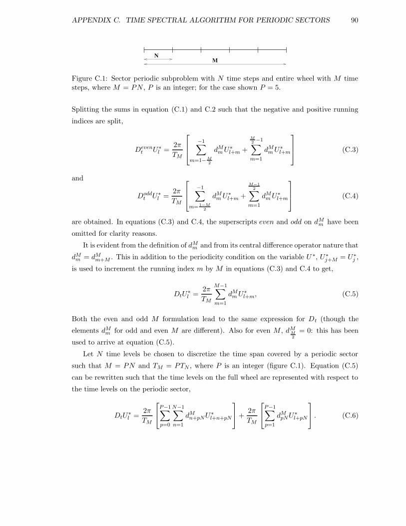
APPENDIX C. TIME SPECTRAL ALGORITHM FOR PERIODIC SECTORS 90
MN
Figure C.1: Sector periodic subproblem with N time steps and entire wheel with M timesteps, where M = PN , P is an integer; for the case shown P = 5.
Splitting the sums in equation (C.1) and C.2 such that the negative and positive running
indices are split,
Devent U∗
l =2π
TM
−1∑
m=1−M2
dMm U∗
l+m +
M2−1
∑
m=1
dMm U∗
l+m
(C.3)
and
Doddt U∗
l =2π
TM
−1∑
m= 1−M2
dMm U∗
l+m +
M−1
2∑
m=1
dMm U∗
l+m
(C.4)
are obtained. In equations (C.3) and C.4, the superscripts even and odd on dMm have been
omitted for clarity reasons.
It is evident from the definition of dMm and from its central difference operator nature that
dMm = dM
m+M . This in addition to the periodicity condition on the variable U ∗, U∗
j+M = U∗
j ,
is used to increment the running index m by M in equations (C.3) and C.4 to get,
DtU∗
l =2π
TM
M−1∑
m=1
dMm U∗
l+m, (C.5)
Both the even and odd M formulation lead to the same expression for Dt (though the
elements dMm for odd and even M are different). Also for even M , dM
M2
= 0: this has been
used to arrive at equation (C.5).
Let N time levels be chosen to discretize the time span covered by a periodic sector
such that M = PN and TM = PTN , where P is an integer (figure C.1). Equation (C.5)
can be rewritten such that the time levels on the full wheel are represented with respect to
the time levels on the periodic sector,
DtU∗
l =2π
TM
P−1∑
p=0
N−1∑
n=1
dMn+pNU∗
l+n+pN
+2π
TM
P−1∑
p=1
dMpNU∗
l+pN
. (C.6)
APPENDIX C. TIME SPECTRAL ALGORITHM FOR PERIODIC SECTORS 91
The second term in this equation represents the contribution from the lth time level on all
other periodic sectors of the annulus. This term will naturally be zero for scalar quantities
(this is shown mathematically later). Note that the p = 0 index is missing in this term,
a direct consequence of the zero contribution from m = 0 index (equation (C.5) or the l th
time level in the computed sector).
If U∗ is a vector and if the time derivative term is being computed for a rotating
component on the wheel, then,
U∗
j+pN = RpU∗
j , (C.7)
where R is the rotation matrix between periodic sectors and Rp = R × R × · · · × R. Thus
equation (C.6) becomes,
DtU∗
l =2π
TM
P−1∑
p=0
N−1∑
n=1
dMn+pNRpU∗
l+n
+2π
TM
P−1∑
p=1
dMpNRpU∗
l
. (C.8)
Introduce two matrix definitions dNn and eN ,
dNn
def=
1
P
P−1∑
p=0
dMn+pNRp
eN def=
1
P
P−1∑
p=1
dMpNRp
(C.9)
then equation (C.8) along with the fact that TM = PTN can be rewritten as,
DtU∗
l =2π
TN
N−1∑
n=1
dNn U∗
l+n +2π
TN
eNU∗
l . (C.10)
where,
dMm =
1
2(−1)m+1 cot
(πm
M
)
M is even
1
2(−1)m+1 cosec
(πm
M
)
M is odd
. (C.11)
For a scalar or non-rotating case, R = I and hence eN = 1P
∑P−1p=1 dM
pN and from the
definition of dMm , the summation amounts to zero, thus eN = 0. Similarly dN
n reduces to the
original definition of the time derivative elements.
Bibliography
[1] A. Jameson. Time Dependent Calculations using Multigrid, with Applications to Un-
steady Flows past Airfoils and Wings. AIAA paper 91-1596, AIAA 10th Computational
Fluid Dynamics Conference, Honolulu, HI, June 1991.
[2] W. R. Briley and H. McDonald. Solution of the Three-Dimensional Compressible
Navier-Stokes Equations by an Implicit Technique, Proc. 4th International Conference
on Numerical Methods in Fluid Dynamics. Lecture Notes in Physics, Springer-Verlag,
pages 105–110, 1974.
[3] R. M. Beam and R. F. Warming. An Implicit Finite-Difference Algorithm for Hy-
perbolic Systems in Conservation Law form. J. Computational Physics, 22:87–110,
1976.
[4] A. Arnone, M. Liou, and L. A. Povinelli. Integration of Navier-Stokes Equations using
Dual Time Stepping and a Multigrid Method. AIAA Journal, 33(6):985–990, June
1995.
[5] C. E. Shannon. Communication in the Presence of Noise. Proceedings of the IRE,
37(1):10–21, January 1949.
[6] J. Yao, A. Jameson, J. J. Alonso, and F. Liu. Development and Validation of a
Massively Parallel Flow Solver for Turbomachinery Flows. J. Propulsion and Power,
17(3):659–668, May 2001.
[7] J. Yao, R. L. Davis, J. J. Alonso, and A. Jameson. Massively Parallel Simulation of the
Unsteady Flow in an Axial Turbine Stage. J. Propulsion and Power, 18(2):465–471,
March-April 2002.
92
BIBLIOGRAPHY 93
[8] R. L. Davis, J. Yao, J. P. Clark, G. Stetson, J. J. Alonso, A. Jameson, C. W. Halde-
man, and M. G. Dunn. Unsteady Interaction Between a Transonic Turbine Stage and
Downstream Components. ASME Turbo Expo, June 2002.
[9] J. M. Verdon and J. R. Casper. A Linearized Unsteady Aerodynamic Analysis for
Transonic Cascades. J. Fluid Mechanics, 149:403–429, 1983.
[10] K. C. Hall, W. S. Clark, and C. B. Lorence. A Linearized Euler Analysis of Unsteady
Transonic Flows in Turbomachinery. ASME J. Turbomachinery, 116(3), 1994.
[11] J. J. Adamczyk. Model Equations for Simulating Flows in Multistage Turbomachinery.
ASME Paper, (85-GT-226), 1988.
[12] L. He. I. Modelling Issues for Computations of Unsteady Turbomachinery Flows; II.
Time-marching Calculations for Blade Row Interaction and Flutter. Unsteady Flows
in Turbomachines, VKI Lecture Series, von Karman Institute for Fluid Dynamics,
Belgium, 1996.
[13] W. Ning and L. He. Computation of Unsteady Flows around Oscillating Blades
using Linear and Nonlinear Harmonic Euler Methods. ASME J. Turbomachinery,
120(3):508–514, 1998.
[14] L. He and W. Ning. Efficient Approach for Analysis of Unsteady Viscous Flows in
Turbomachines. AIAA Journal, 36(11):2005–2012, 1998.
[15] L. He. Three-Dimensional Unsteady Navier-Stokes Analysis of Stator-Rotor Interaction
in Axial-Flow Turbines. IMechE J. Power and Energy, 214:13–22, 2000.
[16] K. C. Hall and E. F. Crawley. Calculation of Unsteady Flows in Turbomachinery using
the Linearized Euler Equations. AIAA Journal, 27(6):777–787, June 1989.
[17] K. C. Hall, C. B. Lorence, and W. S. Clark. Nonreflecting Boundary Conditions for
Linearized Unsteady Aerodynamic Calculations. AIAA Paper 93-0882, 31st Aerospace
Sciences Meeting and Exhibit, Reno, NV, January 11-14 1993.
[18] K. C. Hall and P. D. Silkowski. The Influence of Neighboring Blade Rows on the
Unsteady Aerodynamic Response of Cascades. J. Turbomachinery, 119:85–93, January
1997.
BIBLIOGRAPHY 94
[19] K. C. Hall, J. P. Thomas, and W. S. Clark. Computation of Unsteady Nonlinear Flows
in Cascades using a Harmonic Balance Technique. AIAA Journal, 40(5):879–886, May
2002.
[20] P. D. Silkowski and K. C. Hall. A Coupled Mode Analysis of Unsteady Multistage
Flows in Turbomachinery. J. Turbomachinery, 120:410–421, July 1998.
[21] K. C. Hall and K. Ekici. Multistage Coupling for Unsteady Flows in Turbomachinery.
AIAA Journal, 43(3), March 2005.
[22] M. McMullen, A. Jameson, and J. J. Alonso. Acceleration of Convergence to a Periodic
Steady State in Turbomachinery Flows. AIAA paper 01-0152, AIAA 39th Aerospace
Sciences Meeting, Reno, NV, January 2001.
[23] M. McMullen, A. Jameson, and J. J. Alonso. Application of a Nonlinear Frequency
Domain Solver to the Euler and Navier-Stokes Equations. AIAA paper 02-0120, AIAA
40th Aerospace Sciences Meeting and Exhibit, Reno, NV, January 2002.
[24] J. D. Denton and U. K. Singh. Time Marching Methods for Turbomachinery Flows.
In von Karman Institute Lecture Series 1979-07, 1979.
[25] J. I. Erdos, E. Alzner, and W. McNally. Numerical Solution of Periodic Transonic
Flow through a Fan Stage. AIAA Journal, 15(11), 1997.
[26] J. I. Erdos and E. Alzner. Computation of Unsteady Transonic Flows through Rotating
and Stationary Cascades. Technical report, NASA, 1977. CR 2900.
[27] M. B. Giles. Calculation of Unsteady Wake Rotor Interaction. AIAA J. Propulsion
and Power, 4(4):356–362, 1998.
[28] L. He. An Euler Solution for Unsteady Flows Around Oscillating Blade. ASME J.
Turbomachinery, 112(4):714–722, 1990.
[29] L. He. A Method of Simulating Unsteady Turbomachinery Flows with Multiple Per-
turbations. AIAA Journal, 20(12), 1992.
[30] J. P. Chen and J. W. Barter. Comparison of Time-Accurate Calculations for the
Unsteady Interactions in Turbomachinery Stage. AIAA paper 98-3292, July 1998.
BIBLIOGRAPHY 95
[31] K. Ekici and K. C. Hall. Nonlinear Analysis of Unsteady Flows in Multistage Turbo-
machines using the Harmonic Balance Technique. AIAA paper 06-0422, AIAA 44th
Aerospace Sciences Meeting and Exhibit, Reno, NV, January 9-12 2006.
[32] A. Jameson. Solution of the Euler Equations by a Multigrid Method. Applied Mathe-
matics and Computation, 13:327–356, 1983.
[33] A. Jameson, W. Schmidt, and E. Turkel. Numerical solution of the Euler equations by
Finite Volume methods using Runge Kutta Time Stepping Schemes. AIAA paper 81-
1259, AIAA 14th Fluid and Plasma Dynamics Conference, Palo Alto, CA, June 1981.
[34] A. Jameson. Analysis and Design of Numerical Schemes for Gas Dynamics I: Artificial
Diffusion, Upwind Biasing, Limiters and their Effect on Accuracy and Multigrid Con-
vergence. International J. Computational Fluid Dynamics, 4:171–218, 1995. RIACS
Technical Report 94.15.
[35] A. Jameson. Analysis and Design of Numerical Schemes for Gas Dynamics II: Arti-
ficial Diffusion and Discrete Shock Structure. International J. Computational Fluid
Dynamics, 5:1–38, 1995. RIACS Technical Report 94.16.
[36] B. S. Baldwin and H. Lomax. Thin Layer Approximation and Algebraic Model for
Separated Turbulent Flows. AIAA Paper 78-257, 1978.
[37] Message Passing Interface Forum. MPI: A Message-Passing Interface Standard, March
1994.
[38] S. S. Davis. NACA 64A010 (NASA Ames Model) Oscillatory Pitching. AGARD Report
702, January 1982.
[39] N. A. Pierce and J. J. Alonso. Efficient Computation of Unsteady Viscous Flow by an
Implicit Preconditioned Multigrid Method. AIAA Journal, 36:401–408, 1998.
[40] J. M. Hsu and A. Jameson. An Implicit-Explicit Hybrid Scheme for Calculating Com-
plex Unsteady Flows. AIAA paper 02-0714, AIAA 40th Aerospace Sciences Meeting
and Exhibit, Reno, NV, January 2002.
[41] R. J. Zwaan. Data set 9, LANN Wing, Pitching Oscillation. Agard-R-702 Addendum
No.1, 1985.
BIBLIOGRAPHY 96
[42] W. Haase, E. Chaput, E. Elsholz, M. A. Leschziner, and U. R. Muller. ECARP:
Validation of CFD Codes and Assessment of Turbulence Models; Notes on Numerical
Fluid Mechanics, volume 58. Vieweg, 1997.
[43] C. H. K. Williamson. Vortex Dynamics in the Cylinder Wake. Annual Review Fluid
Mechanics, 28:477–539, 1996.
[44] C. H. K.Williamson. Defining a Universal and Contiguous Strouhal-Reynolds number
relationship of the Laminar Vortex Shedding of a Circular Cylinder. Physics of Fluids,
31:2747–2747, October 1988.
[45] C. H. K.Williamson. Measurements of Base Pressure in the Wake of a Cylinder at Low
Reynolds numbers. Z.Flugwiss, Weltraumforsch,, 14:38–46, 1990.
[46] A. Roshko. On the Development of Turbulent Wakes from Vortex Streets. Technical
report, NACA 1191, January 1954.
[47] R. D. Henderson. Details of the Drag Curve Near the Onset of Vortex Shedding.
Physics of Fluids, 1995.
[48] A. A. Belov. A New Implicit Multigrid-Driven Algorithm for Unsteady Incompressible
Flow Calculations on Parallel Computers. PhD thesis, June 1997. Princeton University.
[49] E. Van der Weide, A. Gopinath, and A. Jameson. Turbomachinery Applications with
the Time Spectral Method. AIAA paper 05-4905, 17th AIAA Computational Fluid
Dynamics Conference, Toronto, Ontario, June 6-9 2005.
[50] Annual ASC Report. http://cits.stanford.edu.
[51] J. J. Reuther, J. J. Alonso, J. C. Vassberg, A. Jameson, and L. Martinelli. An Efficient
Multiblock method for Aerodynamic Analysis and Design on Distributed Memory Sys-
tems. AIAA paper 97-1893, AIAA 13th Computational Fluid Dynamics Conference,
Snowmass, CO, June 1997.
[52] F. Liu and A. Jameson. Cascase Flow Calculations by a Multigrid Euler Method. J.
Propulsion and Power, 9(1):90–97, 1993.
[53] F. Liu and A. Jameson. Multigrid Navier-Stokes Calculations for Three-Dimensional
Cascades. AIAA Journal, 31(10):1785–1791, October 1993.
BIBLIOGRAPHY 97
[54] D. C. Wilcox. Reassesment of the Scale-Determining Equation for Advanced Turbu-
lence Models. AIAA-Journal, 26(11):1299–1310, 1988.
[55] G. Kalitzin. An Efficient and Robust Algorithm for the Solution of the v2-f Turbu-
lence model with Application to Turbomachinery Flow. In WEHSFF 2002 Conference,
Marseille, April 2002.
[56] L. Reed and R. D. Moore. Performance of Single-Stage Axial-Flow Transonic Compres-
sor with Rotor and Stator Aspect Ratios of 1.19 and 1.26, and with design Pressure
Ratio of 1.82. Technical report, NASA, 1978. TP 1338.
[57] S. A. Orszag. On the Elimination of Aliasing in Finite Difference Schemes by Filtering
High-Wavenumber Components. J. Atmospheric Sciences, 1074(28), 1971.
[58] P. R. Spalart and S. R. Allmaras. A One-Equation Turbulence Model for Aerodynamic
Flows. La Recherche Aerospatiale, 1:1–23.
[59] J. C. Vassberg, A. Gopinath, and A. Jameson. Revisiting the Vertical-Axis Wind-
Turbine Design using Advanced Computational Fluid Dynamics. AIAA paper 05-1220,
43rd AIAA Aerospace Sciences Meeting and Exhibit, Reno, NV, January 10-13 2005.
[60] A. Gopinath, P. S. Beran, and A. Jameson. Comparative Analysis of Com-
putational Methods for Limit-Cycle Oscillations. AIAA paper 06-2076, 47th
AIAA/ASME/ASCE/AHS/ASC Structures, Structural Dynamics and Materials Con-
ference, Newport, RI, May 1-4 2006.
[61] C. Canuto, M. Y. Hussaini, A. Quarteroni, and T. A. Zang. Spectral Methods in Fluid
Dynamics; Springer Series in Computational Physics. Springer Verlag, 1988.
[62] P. Moin. ME408: Spectral Methods in Computational Physics. Class notes provided
as part of Stanford’s ME408 Course.
[63] L. N. Trefethen. Spectral Methods in MATLAB. SIAM, 2000.