WP/14/44

Efficient Energy Investment and Fiscal

Adjustment in Senegal

Salifou Issoufou, Edward F. Buffie, Mouhamadou

Bamba Diop, and Kalidou Thiaw

© 2014 International Monetary Fund WP/14/44

IMF Working Paper

Research Department

Efficient Energy Investment and Fiscal Adjustment in Senegal

Prepared by Salifou Issoufou, Edward F. Buffie, Mouhamadou Bamba Diop, and Kalidou Thiaw1

Authorized for distribution by Andrew Berg and Catherine Patillo

March 2014

This Working Paper should not be reported as representing the views of the IMF.

The views expressed in this Working Paper are those of the author(s) and do not necessarily represent

those of the IMF or IMF policy, or of DFID. Working Papers describe research in progress by the

author(s) and are published to elicit comments and to further debate.

Abstract

Senegal's fiscal deficit and public debt have been on the rise in recent years owing partly to an ailing

and inefficient oil-based energy sector. In this paper we use a two-sector, open-economy, dynamic

general equilibrium model to investigate the effects of varying fiscal policy instruments one at a time

and of policy packages that increase public investment in energy and infrastructure in scenarios with

varying degrees of debt finance and with different types of supporting fiscal adjustment. Lowering the

fiscal deficit by raising taxes and cutting government expenditure has adverse effects on growth, real

wages and the supply of public services. Senegal does not need, however, to undertake such difficult

fiscal adjustment. A public investment program that coordinates new investment in low-cost

hydroelectric, coal or gas-fired power with a phased contraction of the oil-based sector raises the total

supply of energy by 70 percent, increases real wages and real GDP, stimulates private investment,

and significantly reduces the fiscal deficit in the medium long term. More aggressive investment

programs borrow against future fiscal gains to combine new energy investments with either delayed

or frontloaded investments in non-energy infrastructure. These programs lead to much higher real

wages and real GDP while keeping public debt sustainable and the fiscal deficit low in the medium

and long term.

JEL Classification Numbers: E62, F34, H63, O43, H54.

Keywords: Energy Reform, Public Investment, Growth, Debt Sustainability, Fiscal Policy, Infrastructure.

Author’s E-Mail Addresses: sissoufou@imf.org; ebuffie@indiana.edu; mbambadiop@gmail.com;

kalidouthiaw@yahoo.fr

1 We thank Andrew Berg, Felipe Zanna, Herve Joly, Olivier Basdevant, and Takuji Komatsuzaki for their useful

comments. This paper is part of a research project on macroeconomic policy in low-income countries supported by

U.K.’s Department for International Development (DFID). This paper should not be reported as representing the

views of the IMF or of DFID. The views expressed in this paper are those of the authors and do not necessarily

represent those of the IMF or IMF policy, or of DFID.

2

Table of Contents Page

I. Introduction ...................................................................................................................................... 3

II. Macroeconomic Developments since 2001: A Brief Overview ...................................................... 4

III. The Model ........................................................................................................................................ 6

III. Model Calibration .......................................................................................................................... 14

IV. Alternative Methods of Fiscal Adjustment ................................................................................... 21

A. Using Traditional Fiscal Instruments to Reduce Fiscal Deficit ................................................ 21

B. Efficient Energy Investment Program and Fiscal Adjustment .................................................. 25

C. Temporarily Raising Official Energy Prices ............................................................................. 28

D. Temporary Borrowing in the Regional Bond Market ............................................................... 29

E. Pushing Harder for Growth: Frontloaded Infrastructure Investment and Aggressive

Borrowing in the Regional versus Eurobond Market ............................................................... 31

VI. Concluding Remarks ...................................................................................................................... 35

Tables

Table 1. Revenue and Expenditure (Period Averages, in percent of GDP) ........................................... 5

Table 2. Calibration of the Model .................................................................................................. 20-21

Table 3. Efficient Energy Investment Program .................................................................................... 26

Table 4. Efficient Energy Investment Program and Delayed Investment in other Infrastructure ........ 28

Table 5. Efficient Energy Investment Program and Frontloaded Investment in other Infrastructure .. 32

Figures

Figure 1. Increasing Profit or Wage Tax Rate ...................................................................................... 22

Figure 2. Cutting Government Consumption of Nontraded Goods ...................................................... 23

Figure 3. Cutting Government Consumption of Traded Goods ........................................................... 24

Figure 4. Efficient Energy Investment Program ................................................................................... 27

Figure 5. Efficient Energy Program and Delayed Non-Energy Investment ......................................... 29

Figure 6. Efficient Energy Program and Delayed Non-Energy Investment: Raising Energy Prices ... 30

Figure 7. Efficient Energy Program and Delayed Non-Energy Investment: Regional Borrowing ...... 31

Figure 8. Efficient Energy Investment and Frontloaded Non-Energy Investment: Regional

Borrowing ............................................................................................................................. 33

Figure 9. Efficient Energy Investment and Frontloaded Non-Energy Investment: Eurobond

Borrowing ............................................................................................................................. 34

Appendix

A. On Public Investment Efficiency, Rates of Return, and Growth ..................................................... 36

B. On Public Investment Efficiency, Rates of Return, and Growth ..................................................... 38

References ........................................................................................................................................... 39

3

I. Introduction

Senegal is experiencing higher �scal de�cits just �ve years after the Heavily Indebted Poor CountriesInitiative (HPIC) cut the stock of total public debt stock from 79 percent of GDP in 2000 to 21percent in 2006. The �scal de�cit has increased from 2:5 percent of GDP in 2001-2006 to an averageof 5 percent of GDP in the last �ve years. Public debt has increased two-fold and is now higher thanits 2006 level. At the same time, the country is grappling with a recurring energy crisis. It needs to�nd a way to both reduce the �scal de�cit and �nance new public investment in energy and non-energyinfrastructure.

Fiscal adjustment is generally di¢ cult and contentious; in practice, easy expenditure cuts andeasy ways to raise revenue are hard to �nd. Senegal has an unusual option, however. The adverseresponse to higher energy prices a couple years ago led to investment in an ine¢ cient oil-based energysector. This has created scope for new investments to both improve e¢ ciency in the energy sector andgenerate �scal surpluses that can be shared with investments in other types of infrastructure and/orhelp pay for de�cit reduction. Reform can be accomplished by investing in an e¢ cient hydropower,gas-�red or coal-�red energy sector while downsizing the ine¢ cient oil-based sector. The critical issueis whether the potential e¢ ciency gains from downsizing the oil-based ine¢ cient sector and replacingit with a more e¢ cient hydropower, gas-�red and coal-�red sector are big enough to allow the countryto both invest more overall in infrastructure and achieve the necessary de�cit reduction.

In this paper we employ a variant of the Fund�s new tool for debt sustainability analysis to analyzethe impact of di¤erent adjustment programs on growth, private investment, real wages, debt, andthe �scal de�cit. The model developed by Bu¢ e et al. (2012) incorporates sector-speci�c capital,productivity-enhancing infrastructure, concessional loans and external commercial debt, a consump-tion VAT and government transfer payments, variable e¢ ciency of public investment, an absorptivecapacity constraint, and poor hand-to-mouth consumers. To adapt the framework for Senegal, we addwage and pro�ts taxes, government consumption of traded and nontraded goods, controlled energyprices, regional CFA-zone debt, an ine¢ cient, oil-based energy sector, and a new, low-cost coal, gasand hydropower energy sector. After investigating the e¤ects of varying policy instruments one ata time, we focus on policy packages that increase public investment in energy and infrastructure inscenarios with varying degrees of debt �nance and with di¤erent types of supporting �scal adjustment.

Our central �nding is that Senegal�s extremely ine¢ cient existing oil-based energy sector representsboth a problem and an opportunity. A public investment program that coordinates new investmentin low-cost hydroelectric power with a phased contraction of the oil-based sector increases the totalsupply of energy by 70 percent while stimulating private investment and increasing real wages andreal GDP. Because technology di¤ers in the oil- and hydro-based sectors, the �scal de�cit increases 1percent of GDP in the short run. In the medium run, however, the investment program delivers �scalgains on the order of 4 percent of GDP. A temporary 30 percent increase in energy prices ensures thatthe �scal de�cit decreases continuously. But this �solution�is problematic �energy prices are alreadyquite high in Senegal. Given the large �scal gains that accrue over the medium term, a strong casecan be made that Senegal should borrow against its �scal surpluses and strongly scale-up investment

4

in infrastructure at the same time that it invests in a more e¢ cient hydro-based energy sector. Thisbig-push investment program increases real wages and real output by more than 10 percent; moreover,the medium-term �scal dividend still exceeds 3 percent of GDP. The program can be �nanced byborrowing either in the regional CFA market or the Eurobond market, but, at current interest rates,borrowing in the Eurobond market is more costly and entails more supporting �scal adjustment.

The rest of the paper is organized into four sections. Section II summarizes macroeconomic devel-opments in Senegal since 2001. Following this, we lay out the model and calibrate it to the data forSenegal in Sections III and IV. In Section V, the heart of the paper, we investigate the pros and consof various strategies of �scal consolidation. Section VI concludes.

II. Macroeconomic Developments since 2001: A Brief Overview

Over the last �ve years Senegal�s �scal position has deteriorated. The budget de�cit averaged 5:1percent of GDP during the 2007-2012 period, up from an average of 2:6 percent for 2001-2006. Therise in the de�cit re�ects the fact that revenues have not kept pace with rising public expenditure(Table 1): relative to 2001-2006, revenue increased by 2.3 percent of GDP, while expenditure rosenearly 5 percent of GDP. Despite the increase in de�cit in recent years, average GDP growth was only4:3 percent during 2007-2012 (compared to 4:4 in the 2001-2006 period) and this sluggish growth hascreated problems in terms of the e¢ ciency of public spending.

A look at the structure of the budget reveals the predominance of current expenditure. Since2001 current expenditure has remained a steady 60 percent of total expenditure (or 15:4 percent ofGDP). Compared to the 2001-2006 period, spending on goods and services (which includes wages andsalaries), total subsidies and other transfers as well as their key component � energy related subsidiesall increased in percent of GDP during the 2007-2012 period. The latter development re�ects anunsettling trend of growing �scal problems in the energy sector. We elaborate on this point below.

5

Table 1. Revenue and Expenditure (Period Averages, in percent of GDP)

Period 2001-2006 2007-2012

Total Revenue and Grants 20:1 22:4

Total Expenditure 22:7 27:5

Current Expenditure 14:0 16:7

Goods and services 8:9 10:8

Subsidies and other current transfers 4:2 4:9

Energy Sector related subsidies** 1:1� 1:8

Capital Expenditure 8:6 10:8

Overall Balance �2:1 �5:1Source: Senegalese authorities and IMF sta¤ estimates

*Average based on 2005-2006 �gures only

**Include fuel, butane and Société Africaine de Ra¢ nage (SAR) subsidies

The challenges facing the energy sector are related to growth as much as they are related to �scal.These challenges stem from an ine¢ cient mode of electricity generation, transmission and distribution,coupled with controlled prices that mask the true costs of power generation.1 About 90 percent of thesector�s power supply is generated using imported oil, with the remaining 10 percent obtained fromhydropower. Benchmark electricity prices, or tari¤s, are set below full cost recovery, giving rise totari¤ gaps and explicit producer and consumer subsidies. As a result, budgetary compensation fromthe government to the state-owned electricity company (SENELEC) amounted to CFAF 105 billionor 1:5 percent of GDP in 2012. Despite these large budgetary transfers, SENELEC has run largeoperating de�cits in recent years. Additional budget costs in the power sector include a shortfall in taxcollection (0:5 percent of GDP), the cost of renting mobile power generators, and expenditure on therehabilitation or extension of existing power plants (0:2 and 0:3 percent of GDP, respectively). Whenthese additional costs are taken into account, the total de�cit of the power sector rises to 2:5 percentof GDP in 2012.2 In addition, power outages, resulting from ine¢ cient production and distribution,have been costly to growth. In 2011, outages are thought to have subtracted 1-1.5 percentage pointof GDP growth.

The costly subsidies in the energy sector, coupled with the negative growth impacts of the ine¢ cientmode of electricity production and distribution, are partly to blame for the recent rapid rise in Senegal�spublic debt. Since 2006, when the HIPC initiative reduced the debt to 21.9 percent of GDP, thetotal public debt increased more than two-fold and currently stands at 45:4 percent of GDP.3 Highergovernment spending on goods and services has also contributed to the increase in public debt.

To stabilize the public debt and avert a potential budget crisis, Senegal must tackle the root causesof its �scal problems. It could cut expenditure on goods and services and/or transfers and subsidies;

1See Torres and others (2011).2June 2013 Senegal Sta¤ Report (IMF Country Report No. 13/170).3Stock at end-2013, IMF Country Report No. 14/4.

6

it could raise revenue by raising taxes, or it could combine both expenditure cuts and tax increasesto reduce its �scal de�cit. Over the medium term, however, the best solution is to reform the energysector by coordinating new investment in a more e¢ cient mode of energy production with gradualdisinvestment in the existing ine¢ cient oil-based energy plants.

III. The Model

The core structure of the model is the same as in Bu¢ e et al. (2012). To adapt the model for Senegal,we add a parastatal energy sector, a regional bond market, and more public sector spending andtax variables. The analysis abstracts from money and nominal rigidities in order to focus on themedium/long-run e¤ects of adjustment on the �scal de�cit and growth.

A lot of notation accompanies any large model. In what follows, x and n subscripts refer tothe tradables and nontradables sectors; k, L, J , E, and z denote capital, labor, land, energy andinfrastructure; Pi is the price of good i; and all quantity variables except labor are detrended by(1 + g)t, where g is the exogenous long-run growth rate of real GDP.

Technology

Firms operate Cobb-Douglas production functions in the tradables and nontradables sectors. In-frastructure enters as a public good that enhances productivity in both sectors, while land is speci�cto the tradables sector:

qx;t = (axz xt�1)k

�xx;t�1J

�JE�xx;tL

1��x��J��xx;t ; (1)

qn;t = (anz nt�1)k

�nn;t�1E

�nn;tL

1��n��nn;t ; (2)

Energy is produced by the state. Initially, all plants employ an ine¢ cient, oil-based technology.In the reform scenarios, these plants are replaced by more e¢ cient coal-�red, gas-�red and/or hydro-electric plants.4 The capital stocks associated with the two technologies are ke (ine¢ cient) and kh(e¢ cient). There is no scope for substitution between inputs and production is constrained by the sizeof the capital stock:

qe;t = aeke;t�1; (3)

qh;t = ahkh;t�1: (4)

Leontief technology also characterizes production of capital goods. Factories and infrastructureare built by combining one imported machine with aj (j = k; z; e; h) units of a nontraded input (e.g.,

4 It is important to note that given the possibly limited potential in sources of hydropower in Senegal, the actualstrategy for investing in an e¢ cient energy sector may focus more on coal- and gas-�red and less on hydropower. Whatis more important, however, is the move to a more e¢ cient mode of electricity production.

7

construction). The supply prices of private capital and infrastructure are thus

Pk;t = Pmm + akPn;t; (5)

Pz;t = Pmm + azPn;t; (6)

Pke;t = Pmm + akePn;t; (7)

Pkh;t = Pmm + akhPn;t; (8)

where Pmm is the price of imported machinery.5

Factor Demands

Competitive �rms maximize pro�ts in the tradables and nontradables sectors by hiring land, labor,and capital up to the point at which the marginal value product of the input equals its price. Laboris intersectorally mobile, but capital is sector speci�c. Hence

Pn;t(1� �n � �n)qn;t=Ln;t = wt; (9)

Px;t(1� �x � �J � �x)qx;t=Lx;t = wt; (10)

Px;t�Jqx;t=Jx = rJ;t; (11)

Px�xqx;t=kx;t�1 = rx;t; (12)

Pn�nqn;t=kn;t�1 = rn;t; (13)

where w is the wage, ri is the capital rental in sector i, and rJ is the land rent.

In the state-run energy sector, Leontief technology implies that employment and purchases of oilare tied to the capital stocks through constants determined by the �xed input-output coe¢ cients:

Lh;t = a2kh;t�1; (14)

Le;t = a3ke;t�1; (15)

Ot = a4ke;t�1: (16)

The price of energy set by the state is far below the notional market-clearing price, P �e . We call P�e

the shadow price and assume e¢ cient rationing of �rm demand. The shadow price and the marginalvalue product of energy are the same therefore in the tradables and nontradables sectors:

Pxqx;t�x=Ex;t = P �e;t; (17)

Pnqn;t�n=En;t = P �e;t: (18)

Private Sector Optimization Problems5The supply price of capital (the cost of building a factory) is the same in the tradables and nontradables sectors.

Once capital is installed, however, it becomes sector-speci�c. Allowing for separate supply prices of capital does notsigni�cantly a¤ect any of the results.

8

The private sector is populated by two types of agents, savers and non-savers. Labor supply ofsavers is �xed at L while that of non-savers is L1 = aL. The two agents are identical qua consumers.Their instantaneous utility function is

U =c1�1=�i

1� 1=� + kocE

1�1=�i

1� 1=� ; i = 1; s;

where � is the intertemporal elasticity of substitution; E is energy consumption; and non-energyconsumption

ci =hk1c

(��1)=�mi + k2c

(��1)=�xi + (1� k1 � k2)c(��1)=�ni

i�=(��1);

is a CES aggregate of traded, nontraded, and imported consumer goods, with substitution parameter� and associated price index

Pt = [k1P1��m;t + k2P

1��x;t + (1� k1 � k2)P 1��n;t ]

1=(1��):

Non-savers consume all of their income each period. Let h, hw, and Pec denote the consumptionvalue added tax (VAT), the tax rate on wage income, and the price of energy sold to households. Sincethe price of energy is arti�cially low, demand is rationed at the level �Ei. Assuming transfers (T ) andremittances (remit) are proportional to the agent�s share in aggregate employment, the non-savers�budget constraint reads6

(1 + ht)Ptc1;t + Pec �E1;t = wtaL(1� hw;t) +a

1 + a(Tt + remit); (19)

or

c1;t =wtaL(1� hw;t) + a(Tt + remit)=(1 + a)� Pec �E1;t

(1 + ht)Pt: (190)

Savers derive income from pro�ts, land rents, wages, transfers, and remittances. They chooseconsumption, government bonds, and investment in physical capital to maximize

1Xt=0

�t

"(cs;t)

1�1=�

1� 1=� + koE1�1=�s;t

1� 1=� + ao(bp;t)

1�1=�

1� 1=�

#; (20)

subject to

bp;t = (1� hp;t)[Pxqx;t + Pn;tqn;t � Pe;t(En;t + Ex;t)� wt(Lx;t + Ln;t)] + wtL(1� hw;t)

+Tt + remit

1 + a+1 + rt�11 + g

bp;t�1 � Ptcs;t(1 + ht)� Pce;tEs;t � �tzt�1;

�Pk;t

"ix;t + in;t +

v

2

�ix;tkx;t�1

� � � g�2

kx;t�1 +v

2

�in;tkn;t�1

� � � g�2

kn;t�1

#; (21)

(1 + g)kx;t = ix;t + (1� �)kx;t�1; (22)

(1 + g)kn;t = in;t + (1� �)kn;t�1; (23)

Es;t � �Es;t; (24)

6Taxes on energy are included in Pec.

9

where � = 1=[(1+ �1)(1+ g)(1��)=� ] is the discount factor; �1 is the pure time preference rate; � is the

intertemporal elasticity of substitution; bp is bonds purchased by domestic residents; hp is the pro�tstax; ij is gross investment in sector j; � is the depreciation rate; r is the interest rate on tradablebonds sold in the regional WAEMU market; and � is the user fee charged for infrastructure services.Bonds generate non-pecuniary services, and the terms v(�)kj;t�1=2 in the budget constraint measureadjustment costs incurred in changing the capital stock. Observe also that the trend growth rateappears in several places in (21)-(23), re�ecting the fact that some variables are dated at t and othersat t-1.7

The choice variables in the optimization problem are cs;t, bp;t, Es;t, ij;t, and kj;t. On an optimalpath,

cs;t = cs;t+1

"ao

�bp;tPt

��1=�c1=�s;t+1(1 + ht) +

��11 + rt1 + g

PtPt+1

1 + ht1 + ht+1

�#��; (25)

FPk;tPk;t+1

�1 + v

�ix;tkx;t�1

� � � g��

=rx;t+1(1� hp;t+1)

Pk;t+1+ 1� �

+v

�ix;t+1kx;t

� � � g��

ix;t+1kx;t

+ 1� ��

�v2

�ix;t+1kx;t

� � � g�2

; (26)

FPk;tPk;t+1

�1 + v

�in;tkn;t�1

� � � g��

=rn;t+1(1� hp;t+1)

Pk;t+1+ 1� �

+v

�in;t+1kn;t

� � � g��

in;t+1kn;t

+ 1� ��

�v2

�in;t+1kn;t

� � � g�2

; (27)

koE�1=�s;t = Pce;t

c�1=�s;t

Pt(1 + ht)+ �4;t; (28)

�4;t(Es;t � �Es;t) = 0 (29)

where

F ��

cs;tcs;t+1

��1=� Pt+1Pt

1 + ht+11 + ht

1 + g

�1

and �4 is the multiplier attached to the rationing constraint (24). These are generally familiar con-ditions. The Euler equations in (25)-(27) govern the paths of non-energy consumption and sectoralinvestment. Equations (28) and (29) state that the relative price of energy (Pec=P ) is less than themarginal rate of substitution between energy consumption and non-energy consumption when demandis rationed (i.e., �4;t > 0).

7The convention for detrending the capital stocks di¤ers from that for other variables. Because Kj;t�1 (the capitalstock before detrending) is the capital stock in use at time t, we de�ne kj;t�1 � Kj;t�1=(1 + g)

t. Under this convention,ij = (� + g)kj in the long run � as required for the capital stock to grow at the trend growth rate g.

10

In passing we should say a few words about the assumption that bonds yield non-pecuniary services.This is not to everyone�s taste. It is essential, however, for realistic calibration of the model. Notefrom (25-(27) that

aob�1=�P (1 + h)

c�1=�s

= 1� �1(1 + r)

1 + g;

ri(1� hp)Pk

� � =1 + g

�1� 1; i = x; n

at the initial steady state. When bonds do not confer non-pecuniary services, the real after-tax returnon private capital is constrained to equal the real interest rate r paid on government bonds. Butr is only 3.5 percent , whereas the return on capital is probably on the order of 8-10 percent . Ifnon-pecuniary bene�ts do not enter as a wedge between the �nancial returns, then the model wouldhave to be calibrated either with an unrealistically high real interest rate or with an unrealisticallylow return on private capital (implying, also, absurdly high values for the capital-ouput ratio and theshare of investment in GDP).

Exact Price Indices

Accurate measurement of real wages requires exact consumption price indices for saving and non-saving households. So far, all we have is the formula for P , the exact price index for non-energyconsumption. To derive the exact price indices for aggregate consumption, we also need the shadowprices of E1 and Es. For households that save, the shadow price is the price at which �4 = 0 inequation (28):

P �ec;t = ko

� �Es;tcs;t

�Pt(1 + ht): (30)

The exact price index paired with P �ec is

CPI�s;t =�P 1��t + k�o (P

�ec;t)

1�� �1=(1��) : (31)

With P �ec and CPI�s in hand, it is easy to show (see Appendix A) that

CPIs;t =CPI�s;t

1 + e;t(P�ec;t � Pec;t)=Pec;t

; (32)

where e;t � Pec;t �Es;t=(Ptcs;t + Pec;t �Es;t), the share of energy in aggregate consumption measured ato¢ cial prices.

Since savers and non-savers are identical qua consumers,

CPI1;t =CPI�1;t

1 + e1;t(P�ec;t � Pec;t)=Pec;t

; (33)

11

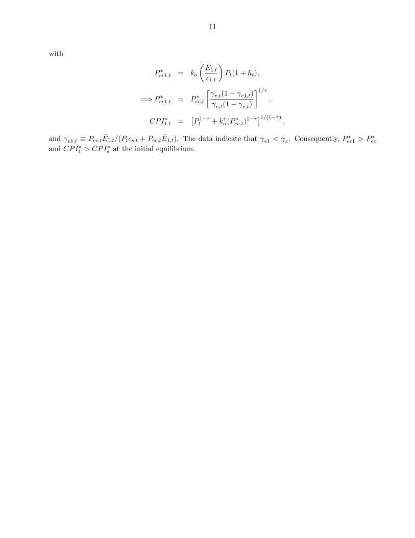
with

P �ec1;t = ko

� �E1;tc1;t

�Pt(1 + ht);

=) P �ec1;t = P �ec;t

� e;t(1� e1;t) e;t(1� e;t)

�1=�;

CPI�1;t =�P 1��t + k�o (P

�ec;t)

1�� �1=(1��) ;and e1;t � Pec;t �E1;t=(Ptcs;t + Pec;t �E1;t). The data indicate that e1 < e. Consequently, P

�ec1 > P �ec

and CPI�1 > CPI�s at the initial equilibrium.

12

Public Investment

The capital stocks in the energy sector increase over time at the rates

(1 + g)ke;t = ie;t + (1� �)ke;t�1; (34)

(1 + g)kh;t = ih;t + (1� �)kh;t�1; (35)

where ie and ih denote gross investment.

Public investment is seldom perfectly e¢ cient. As noted in the introduction, ine¢ ciency in theenergy sector takes the form of excessive reliance on high-cost, oil-based technology. In the case ofinfrastructure, we allow for the possibility that increases in the stock of physical capital ~z may nottranslate into equal increases in the stock of economically valuable capital z.8 The usual law of motionapplies to ~z

(1 + g)~zt = iz;t + (1� �)~zt�1; (36)

but some of the newly built infrastructure may not enhance productivity:

zt = zo + s(~zt � ~zo); s � 1: (37)

Fiscal Adjustment and the Public Sector Budget Constraint

Government expenditure comprises transfers, wages, oil imports, investments in energy and in-frastructure, interest payments on the debt, supplemental energy imports9 qf from Mali at price Pf ,and purchases gn and gm of nontraded and imported goods. Revenues �ow from user fees assessedfor infrastructure services, the consumption VAT, taxes on wages and pro�ts, grants (x), and energysales. When expenditure exceeds revenues, the resulting de�cit is �nanced by issuing additional debtb in the regional bond market:10

bt � bt�1 = Pz;t

"�1 +

iz;t~zt�1

� � � g��(iz;t � iz;o) + iz;o

#+ Pke;tie;t + Pkh;tih;t

+Pn;tgn;t + Pm;tgm;t +rd � g1 + g

dt�1 +rdc � g1 + g

dct�1 +rt�1 � g1 + g

bt�1 + Tt + wt(Le;t + Lh;t)

+Po;tOt + Pf;tqf;t � Pec;t(Es;t + �E1;t)� Pe;t(Ex;t + En;t)� htPt(ct + c1;t)� xt � �tzt�1�hw;twtL(1 + a)� hp;t[Pxqx;t + Pn;tqn;t � Pe;t(En;t + Ex;t)� wt(Lx;t + Ln;t)]: (38)

Plans to replace the oil-based energy sector with new, more e¢ cient sources of energy have been inthe works for years. We assumed they can be implemented e¢ ciently utilizing SENELEC�s existing

8See Hulten (1996) and Pritchett (2000) for evidence that public investment often fails to increase the supply ofproductive infrastructure.

9These imports are through OMVS (Organization pour la Mise en Valeur du Fleuve Senegal) which is a regionalorganization that comprises Mali, Mauritania and Senegal).10When concessional and non-concessional borrowing supplement borrowing in the regional bond market, dt + dct �

dt�1 � dct�1 is added on the left side in equation (38).

13

personnel. Accordingly, capital outlays in the energy sector are simply the product of the supply priceof energy and planned gross investments.

The story for infrastructure investment is di¤erent. Due to the scarcity of technical expertiseand skilled administrators, there is a risk of large cost overruns in ambitious programs that scale upinvestment too quickly in too many areas. To capture this, we multiply new investment (iz;t� iz;o) by(1 + iz;t=~zt�1 � � � g)�, where � � 0 determines the severity of the the absorptive capacity constraintin the public sector. The constraint a¤ects only implementation costs for new projects: in a steadystate, (iz;t=~zt�1 � � � g)� = 1 as iz;t=~zt�1 = � + g.

Senegal is interested mainly in how alternative programs of investment + �scal adjustment a¤ectgrowth and the �scal de�cit. The technical problem in analyzing such scenarios is that the debtdynamics associated with an exogenously speci�ed program are unstable. Fortunately, the problemadmits of a simple solution. Because transfers are purely lump sum, variations in T do not a¤ect anyother variable in the model. Consequently, if we assume that transfers adjust to continuously balancethe budget, the paths for the real wage, real GDP, private investment, etc., re�ect only the impact ofthe speci�ed program, while the solution for

To � Tt = Pz;t

"�1 +

iz;t~zt�1

� � � g��(iz;t � iz;o) + iz;o

#+ Pke;tie;t + Pkh;tih;t

+Pn;tgn;t + Pm;tgm;t +rd � g1 + g

dt�1 +rdc � g1 + g

dct�1 +rt�1 � g1 + g

bt�1 + To + wt(Le;t + Lh;t)

+Po;tOt + Pf;tqf;t � Pec;t( �Es;t + E1;t)� Pe;t(Ex;t + En;t)� htPt(ct + c1;t)� xt � �tzt�1�hw;twtL(1 + a)� hp;t[Pxqx;t + Pn;tqn;t � Pe;t(En;t + Ex;t)� wt(Lx;t + Ln;t)]: (39)

mirrors the change in the path of the �scal de�cit.

Immediate de�cit reduction is a priority in Senegal.11 Given the current low cost of borrowing in theregional bond market, however, the government should consider the tradeo¤s a¤orded by temporaryde�cit-�nanced programs. In these programs, one or more policy instruments adjust gradually toeliminate the �scal de�cit and stabilize the path of debt. See Appendix B for more details and anillustrative example.

Market-Clearing Conditions

Wages and prices adjust to align demand with supply in the markets for labor and nontraded

11The Senegalese authorities have made �scal reduction a priority and a commitment.

14

goods:

L(1 + a) = Lx + Ln + Le + Lh; (40)

qn;t = (1� k1 � k2)(Pn;t=Pt)��(cs;t + c1;t) + gn;t+ak

hix;t ++

v

2(�)2kx;t�1 + in;t +

v

2(�)2kn;t�1

i+ akeie;t

+akhih;t + az

"�1 +

iz;t~zt�1

� � � g��(iz;t � iz;o) + iz;o

#: (41)

In the energy sector, where low prices and acute shortages are the norm, rationing constraints purchasesto equal available supply:

qe;t + qh;t + qf;t = Ex;t + En;t + Es;t + E1;t: (42)

External Debt Accumulation and the Current Account

Summing the budget constraints of private agents and the government produces the nationalsaving-investment identity

bf;t � bf;t�1 = Pt(cs;t + c1;t) + Pz;t

"�1 +

iz;t~zt�1

� � � g��(iz;t � iz;o) + iz;o

#+Pk;t

hix;t + in;t +

v

2(�)2kx;t�1 +

v

2(�)2kn;t�1

i+ Pke;tie;t + Pkh;tih;t

+rd � g1 + g

dt�1 +rdc � g1 + g

dct�1 +rt�1 � g1 + g

bf;t�1 + Po;tOt + Pf;tqf;t

+Pn;tgn;t + Pm;tgm;t � Pn;tqn;t � Pxqx;t � xt � remit; (43)

where bf � b� bp. Senegal�s net foreign debt, bf , equals its net position in WAEMU tradable bonds.This increases each year by the di¤erence between national spending and national income.

Interest Rate Determination

Senegal is a large player in the regional bond market: when it borrows more, it pushes up theequilibrium interest rate. Rather than build a general equilibrium model of the regional economy, wepostulate a simple inverse loan supply curve:

rt = ro + �

�bf;t � bf;obf;o

�; � � 0: (44)

IV. Model Calibration

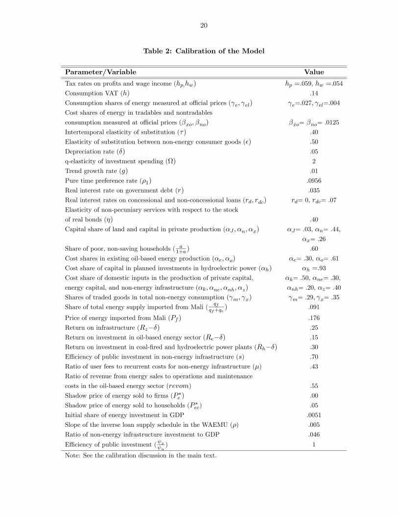
A mix of hard data supplied by the Senegalese government, empirical estimates from the developmentliterature, and judgment were employed to calibrate the model. Below we discuss seriatim the rationaleand the data sources for the value assigned to each parameter in Table 2:

15

� Tax rates on pro�ts and wage income (hp, hw). Revenue from income taxes was 5.6 percentof GDP in 2012, with wage taxes accounting for 60 percent of the total. This and the incomeshares of wages and pro�ts at the initial equilibrium imply an e¤ective tax rate of 5.9 percenton pro�ts and 5.4 percent on wages. The e¤ective rates are much lower than the statutory ratesbecause the base for income taxes is a small fraction of GDP (roughly the share of the formalsector in total output).

� Consumption value-added tax (h). The consumption VAT in the model proxies for the averageindirect tax rate. Total tax revenue amounted to 18.9 percent of GDP in 2011. Subtractingincome taxes and taxes on petroleum products brings the �gure down to 10.7 percent . Dividingthis by the share of private consumption in GDP yields 14 percent.12

� Consumption shares of energy measured at o¢ cial prices ( e, e1). Household survey data for2005-2006 put the share of energy in consumption at 2.1 percent overall and at 0:4 percent forthe poorest three deciles. Lacking more recent data, we assumed the consumption share for poor,non-saving households is still 0.4 percent. This and the �gure for the aggregate consumptionshare give a share of 2.7 percent for non-poor households.

� Cost shares of energy in tradables and nontradables production, measured at o¢ cial prices (�xo,�no). Data from SENELEC on sales of energy to �rms vs. households together with the datafor the share of energy in consumption and the ratio of consumption to GDP allow us to backout guesstimates of the cost shares of energy in private production, measured at o¢ cial prices.Absent any information on the relative energy intensity of tradables vs. nontradables production,we set the cost share at 1.25 percent in both sectors. Sales to �rms then comprise 44 percent oftotal energy sales at the initial equilibrium.13

� Intertemporal elasticity of substitution (�). Most estimates of � for LDCs lie between .20 and .75(Agenor and Montiel, 1996). The assigned value of .40 is in the middle of this range and closeto the estimates for Africa in Ostry and Reinhart (1992) and for Ghana and Kenya in Ogaki etal. (1996).

� Elasticity of substitution between non-energy consumer goods (�). Estimates of demand systemswith 5-10 goods generally place compensated own-price elasticities of demand in the .15-.50range.14 A value of .50 for � produces compensated own-price elasticities in the lower/middlepart of this range.

� Depreciation rate (�). There is little hard data on depreciation rates in LICs. Our choice of 5percent is in line with estimates for developed countries.15

12Despite the inclusion of revenue from other indirect taxes, the e¤ective rate is well below the statutory VAT rate.This re�ects the fact that a substantial part of private consumption escapes the tax net.13The slight upward revision relative to the data (44 percent vs. 37 percent) takes into account energy consumption at

owner-occupied businesses.14See Lluch et al. (1977, chapter 3), Deaton and Muellbauer (1980, p.71), Blundell (1988, p.35), and Blundell,

Pashardes, and Weber (1993, Table 3b, p.581).15A depreciation rate of 5% is in line with empirical estimates of the depreciation rate for physical capital (Blundell et

al., 1992; Nadiri and Prucha, 1996) and with data on service lives of equipment and structures reported by the Bureauof Economic Analysis (Musgrave, 1992). Papers that use a higher depreciation rate of 10% explicitly or implicitly count

16

� q-elasticity of investment spending (). Evaluated at the initial equilibrium, the elasticity ofinvestment with respect to Tobin�s q is = 1=(�+g)v, where v is the parameter that determinesadjustment costs to changing the capital stock. There are no reliable estimates of this elasticityfor LDCs. The assigned value, 2, is at the high end of estimates for developed countries. Theresults do not change substantively when equals .5 or 10.

� Trend growth rate (g). The trend growth in per capita income is a modest 1 percent.

� The pure time preference rate (�1) and the real return on capital. We chose the pure timepreference rate jointly with the trend growth rate, the pro�ts tax, and the intertemporal elasticityof substitution so that the after-tax return on capital equals 10 percent.16

� Real interest rate on government debt (r). Over the past decade, the real interest rate on bondsthe Government of Senegal (GOS) sells in the WAEMU market has averaged 3.5 percent .

� Real interest rates on concessional and non-concessional loans (rd, rdc). The average real interestrate on concessional loans is approximately zero. In Senegal�s most recent Eurobond issue, theinterest rate was 7 percent.

� Elasticity of non-pecuniary services with respect to the stock of real bonds (�). The parameter� governs the semi-elasticity of bond demand with respect to the real interest rate, while theratio �=� �xes the long-run elasticity of bond holdings with respect to a permanent increase inprivate income (of saving households).17 We set � equal to � on the assumption that unity is areasonable value for the income elasticity.

� Cost shares of land and capital in private production (�J , �n, �x). The cost shares of capital inthe nontradables sector and the non-agricultural part of the tradables sector were computed fromdata in the national income accounts. Unfortunately, no data are available for the agriculturalpart of the tradables sector. We decided to rely therefore on the factor shares reported for SSA insocial accounting matrices assembled by GTAP (Global Trade Assistance Project). The simpleaverage of the shares in smallholder and commercial agriculture is .19 for capital and .14 forland.18 The capital-labor ratio in agriculture is 54 percent of that in non-agriculture vs. 49.3percent in nearby Cameroon (Emini et al., 2006). The cost shares in Table 1 for the compositetradables sector are a weighted average of the shares in the non-agricultural and agriculturaltradables sectors.

� Share of poor, non-saving households [a=(1 + a)]. There are no estimates of the share of non-saving households in Senegal or other LDCs. Our guesstimate, 60 percent, is at the high end ofestimates for developed countries.

consumer durables as part of investment. While this is conceptually correct, it is inappropriate in a model that focuseson how changes in the physical capital stock a¤ect GDP growth, tax revenues, and real wages.16Across steady states, the after-tax real return on private capital equals (1 + �1)(1 + g)

� � 1. The after-tax return isset directly as r1 in the computer programs.17Bond demand is a function of consumption and the real interest rate. In the long run, the change in consumption

equals the change in real income.18We have converted the GTAP value added shares into cost shares. The labor share is determined residually after

computing the cost share of energy at the shadow price of energy.

17

� Cost shares in existing oil-based energy production (�e, �o). SENELEC has provided us withdata on labor costs, energy costs , and depreciation charges. Straightforward algebra shows thatthe cost share of oil is

�o =J�=Re

1� (1 + F )J(1� �=Re);

where J is oil�s share in O+M, F is the ratio of wages to oil expenditure, and Re is the grossreturn on energy investment.19 The average values of J and F for 2005-2010 were .79 and .14,respectively. These numbers and the values assigned to � and Re give cost shares of .61 for oil,.09 for labor, and .30 for capital.

� Cost share of capital in planned investments in hydroelectric power (�h). The value added shareof capital in the ine¢ cient oil-based energy sector is 78 percent . Production of hydroelectricpower is even more capital intensive. The Ministry of Energy estimates the cost share of capitalin planned investments at 93 percent.

� Cost share of domestic inputs in the production of private capital, energy capital, and non-energyinfrastructure (�k; �ne; �nh; �z). The cost share of domestic inputs in the production of capitalgoods for the private sector is 50 percent , a guesstimate based on observed values in other LDCs.Investment in energy and non-energy infrastructure is much more import intensive. The costshares �ne, �nh, and �z come from data on past projects undertaken by the Ministry of Energyand the Ministry of Infrastructure and Transports.

� Shares of traded goods in total non-energy consumption ( m, x). Traded consumer goods inthe model are divided into non-competitive imports and domestically produced tradable goods.Unsurprisingly, the data say that Senegal is a highly open economy: the combined share oftradable goods in total non-energy consumption is 64 percent.20

� Power imported from Mali (qf , Pf ). Nine percent of total energy supply is imported from ahydropower plant in Mali at a price of 21 CFA/kWh � 17.6 percent of the average domestictari¤ and 13 percent of O+M costs at SENELEC plants.21

� Return on infrastructure (Rz � �). Estimates of the return on infrastructure are all over themap, but the weight of the evidence in both micro and macro studies points to a high averagereturn. The median rate of return on World Bank projects circa 2001 was 20 percent in SSA and15-29 percent for various sub-categories of infrastructure investment. In the Bank�s recently-completed, comprehensive study of infrastructure in Africa, estimated returns for electricity,water and sanitation, irrigation, and roads range from 17 percent to 24 percent (Foster and

19J = PoO=(�PkeKe + wLe + Po). When the capital rental is computed at the shadow price of energy, this can bewritten as

J =�o

(�=Re)�e + �o(1 + F );

=) �o =J�=Re

1� (1 + F )J(1� �=Re);

as �e = 1� �L � �o = 1� �o(1 + F ).20The weight in the CPI is 62.7% when energy consumption is measured at o¢ cial prices.21These imports are through OMVS (Organization pour la Mise en Valeur du Fleuve Senegal) which is a regional

organization that comprises Mali, Mauritania and Senegal).

18

Briceno-Garmendia, 2010, chapter 2). Similarly, the macro-based estimates in Dalgaard andHansen (2005) cluster between 15 percent and 30 percent for a wide array of di¤erent estimators.Hulten et al. (2006), Escribano et al. (2008), Calderon et al. (2009), and Calderon and Serven(2009) supply additional evidence of high returns.

In keeping with this evidence, we assume the return on infrastructure (net of depreciation)equals 25 percent in the base case.

� Return on investment in the oil-based energy sector (Re � �). The return on investment in theoil-based energy sector is 15 percent. This number might seem too high. It is consistent, however,with the perception that oil-based plants su¤er from a high degree of technical ine¢ ciency. Thereturn is a respectable 15 percent only because power is scarce and its shadow price extremelyhigh. E¢ cient energy investments pay a much higher return.

� Return on investment in coal-�red + hydroelectric power plants (Rh � �). The return on invest-ment in e¢ cient coal-�red + hydroelectric power plants is set at 30 percent . This is consistentwith the high shadow price of energy in the model and with estimates of cost savings fromreplacing less e¢ cient with more e¢ cient plants. As noted earlier, the price Senegal pays topurchase power from the jointly operated hydropower plant in Mali is only 13 percent of O+Mcosts at SENELEC�s oil-based plants. In our calibration, O+M costs at new hydropower plantsare 26.3 percent of O+M costs at existing oil-based plants. This suggests that an initial returnof 30 percent is, if anything, too conservative.22

� E¢ ciency of public investment in non-energy infrastructure (s). Casual observation and theempirical estimates in Hulten (1996) and Pritchett (2000) suggest that public investment isine¢ cient in many LICs. Accordingly, our base case assumes that 30 percent of public invest-ment fails to increase the stock of productive infrastructure (s = :7). The e¤ective return oninfrastructure investment is thus 17.5 percent .

� Ratio of user fees to recurrent costs per unit of non-energy infrastructure (�). On average, userfees cover 43 percent of recurrent costs for non-energy infrastructure. The number was computedby the GOS. It is slightly lower than the average for SSA reported (50 percent ) reported inBricendo-Garmendia (2008).

� Ratio of revenue from energy sales to operations and maintenance costs in the oil-based energysector (revom). After adjustment for transmission and distribution losses, the ratio of the averagetari¤ to per unit operations and maintenance costs was .72 in 2011. But inclusion of "uncountedlosses" from theft and "ine¢ cient collection of bills" reduces the �gure to .55. The resultingrevenue shortfall is 2 percent of GDP in the data and 1.97 percent in the model.

� The shadow price of energy sold to �rms (P �e ) and the initial share of oil-based energy investmentin GDP. Values for these two variables are derived residually from the values assigned to the costshare of capital in oil-based energy production (�e), the depreciation rate (�), the trend growthrate (g), the gross return on investment in oil-based energy (Re), the cost shares of energy in

22 It should be emphasized, again, that 30% is the return measured at the initial high shadow price of energy. Thereturn measured at the o¢ cial price, which is still quite high compared to prices elsewhere in WAEMU and SSA, is11.6%.

19

private production (�xo, �no), the ratio of revenue to operations and maintenance costs (revom),and the average power tari¤ (Pe;avg). Pen and paper math give

ie =P �e (� + g)�eqe

Re;

Pe;avgP �e

= revom[1� �e(1� �=Re)];

where qe is domestically produced energy sales and ie is gross energy investment. We chooseunits so that Pe;avg = 1. Our choices for other variables then return P �e = 2:59 and a share ofenergy investment in GDP of .51 percent .23,24

� Shadow price of energy sold to households (P �ec). Needless to say, there is no data that bears onthe likely shadow price of energy sold to households. We simply assume the shadow price is thesame as for energy sold to �rms (P �ec = P �e ).

� Slope of the inverse loan supply schedule in the WAEMU (�). The parameter � determines howmuch the interest rate rises when the GOS issues more debt in WAEMU. We assume demand isfairly elastic; the value �xed for � says that additional debt sales equal to 6 percent of GDP (adoubling in the stock of debt) would raise the real interest rate from 3.5 percent to 5 percent.

� Elasticities of sectoral output with respect to the stock of infrastructure ( x; n). The ratio x= n is set independently. This ratio and other values assigned in calibrating the model �most notably, the return on infrastructure � pin down n and x. We assume x= n = 1 inall runs.

� Government purchases of imported and nontraded goods (gm, gn), non-energy infrastructureinvestment (Iz), remittances (remit), government bonds held by foreign investors (bf ), govern-ment bonds held by domestic residents (bp), concessional debt (d), and non-concessional debt( dc). The GOS collects data on all of these variables. The values in Table 1 are for 2012.

23The price of energy sold to households and �rms equals unity at the initial equilibrium. In fact, households arecharged a slightly higher price than �rms. All that matters in the simulations, however, is the increase in the price, notits initial level.24 Investment at SENELEC was 1:4 percent of GDP in 2012. But purchases from private power companies currently

account for 47 percent of SENELEC�s sales. If investment at private suppliers is comparable to that at SENELEC, thentotal energy investment is around 2:8 percent of GDP.

20

Table 2: Calibration of the Model

Parameter/Variable Value

Tax rates on pro�ts and wage income (hp;hw) hp =.059, hw =.054

Consumption VAT (h) .14

Consumption shares of energy measured at o¢ cial prices ( e; el) e=.027; el=.004

Cost shares of energy in tradables and nontradables

consumption measured at o¢ cial prices (�xo; �no) �xo= �no= .0125

Intertemporal elasticity of substitution (�) .40

Elasticity of substitution between non-energy consumer goods (�) .50

Depreciation rate (�) .05

q-elasticity of investment spending () 2

Trend growth rate (g) .01

Pure time preference rate (�1) .0956

Real interest rate on government debt (r) .035

Real interest rates on concessional and non-concessional loans (rd; rdc) rd= 0, rdc= .07

Elasticity of non-pecuniary services with respect to the stock

of real bonds (�) .40

Capital share of land and capital in private production (�J ; �n; �x) �J= .03, �n= .44,�x= .26

Share of poor, non-saving households ( a1+a) .60

Cost shares in existing oil-based energy production (�e; �o) �e= .30, �o= .61

Cost share of capital in planned investments in hydroelectric power (�h) �h =.93

Cost share of domestic inputs in the production of private capital, �k= .50, �ne= .30,

energy capital, and non-energy infrastructure (�k; �ne; �nh; �z) �nh= .20, �z= .40

Shares of traded goods in total non-energy consumption ( m; x) m= .29; x= .35

Share of total energy supply imported from Mali (qf

qf+qe) .091

Price of energy imported from Mali (Pf ) .176

Return on infrastructure (Rz��) .25

Return on investment in oil-based energy sector (Re��) .15

Return on investment in coal-�red and hydroelectric power plants (Rh��) .30

E¢ ciency of public investment in non-energy infrastructure (s) .70

Ratio of user fees to recurrent costs for non-energy infrastructure (�) .43

Ratio of revenue from energy sales to operations and maintenance

costs in the oil-based energy sector (revom) .55

Shadow price of energy sold to �rms (P �e ) .00

Shadow price of energy sold to households (P �ec) .05

Initial share of energy investment in GDP .0051

Slope of the inverse loan supply schedule in the WAEMU (�) .005

Ratio of non-energy infrastructure investment to GDP .046

E¢ ciency of public investment ( x n) 1

Note: See the calibration discussion in the main text.

21

Table 2: Calibration of the Model (continued)

Parameter/Variable Value

Ratios of government purchases of imported and nontraded goods to GDP gm= .009, gn= .043

Ratios of government bonds held by foreign investors (bf ),

domestic investors to initial GDP (bp) to initial GDP, bf= .06, bp= .063,

Ratios of concessional debt (d), and non-concession debt to initial GDP(dc) d= .292, dc= .035

Absorptive capacity parameter (') 0.00

Note: See the calibration discussion in the main text.

V. Alternative Methods of Fiscal Adjustment

A. Using Traditional Fiscal Instruments to Reduce Fiscal De�cit

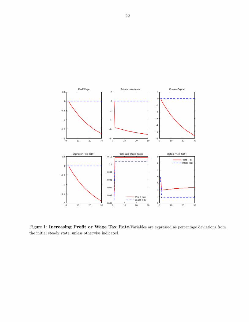
We begin by analyzing the implications of using traditional �scal instruments to reduce the �scalde�cit. In business-as-usual �scal adjustment, the government alters tax rates or its level of spending.We look speci�cally at the e¤ects of (i) raising wage or pro�t taxes and (ii) reducing governmentconsumption of traded or nontraded goods.

Increasing the wage tax a¤ects only the �scal de�cit. There are no real e¤ects as the change inthe tax is equivalent to a one-o¤ lump sum tax.25 Raising the tax rate by 5 percentage points reducesthe �scal de�cit from 5:9 percent of GDP to slightly below 3 percent of GDP (Figure 1). Increasingthe pro�t tax is �scally inferior to increasing wage tax. The de�cit decreases less owing to the factthat pro�ts are a smaller share of GDP than wages. Moreover, a higher pro�t tax reduces privateinvestment and capital stock, leading to lower GDP and a loss of revenue from other sources (Figure1).

Although raising the pro�t tax is distributionally less objectionable than raising the wage tax, itgenerates a smaller revenue gain and engenders contractionary real e¤ects that are avoided with thewage tax increase. Note in this connection that part of the pro�t tax is e¤ectively paid by workers:on the transition path, decreases in the capital stock continuously contract the demand for labor; inthe long run, this reduces the real wage 2:5 percent.

Cutting government consumption of nontraded goods raises real wages and reduces �scal de�cit.It produces contractionary e¤ects, however, on private investment, the capital stock, and real GDP,thereby reducing revenue from other sources (Figure 2).

25The wage tax is a lump-sum tax because labor supply is assumed to be completely inelastic for both saving andnon-saving households. Assuming elastic labor supply could change the ranking of wage vs. pro�ts taxes. Althoughmacro and micro estimates of the Frisch elasticity di¤er greatly, the weight of the evidence supports the view that laborsupply is inelastic. Keane and Rogerson (2011) observe, for example, that "the majority of the economics profession hascome to the conclusion that labor supply elasticities are small; and, in particular, that labor supply is not very responsiveto tax changes".

22

0 10 20 30­2

­1.5

­1

­0.5

0

0.5Real Wage

0 10 20 30­8

­6

­4

­2

0

2Private Investment

0 10 20 30­6

­5

­4

­3

­2

­1

0

1Private Capital

0 10 20 30­2

­1.5

­1

­0.5

0

0.5Change in Real GDP

0 10 20 300.05

0.06

0.07

0.08

0.09

0.1

0.11Profit and Wage Taxes

Profit TaxWage Tax

0 10 20 302

3

4

5

6

7

8

9Deficit (% of GDP)

Profit TaxWage Tax

Figure 1: Increasing Pro�t or Wage Tax Rate.Variables are expressed as percentage deviations fromthe initial steady state, unless otherwise indicated.

23

0 10 20 300

0.2

0.4

0.6

0.8

1Real Wage

0 10 20 30­1

­0.8

­0.6

­0.4

­0.2

0Private Investment

0 10 20 30­1

­0.8

­0.6

­0.4

­0.2

0Private Capital

0 10 20 30­1

­0.8

­0.6

­0.4

­0.2

0Change in Real GDP

0 10 20 302

2.5

3

3.5

4

4.5

5Government Consumption

Non­Traded Goods

0 10 20 302

3

4

5

6

7

8

9Deficit (% of GDP)

Figure 2: Cutting Government Consumption of Nontraded Goods.Variables are expressed aspercentage deviations from the initial steady state, unless otherwise indicated.

24

0 10 20 30­1

­0.8

­0.6

­0.4

­0.2

0Real Wage

0 10 20 300

0.1

0.2

0.3

0.4

0.5

0.6

0.7Private Investment

0 10 20 300

0.05

0.1

0.15

0.2

0.25

0.3

0.35

0.4Private Capital

0 10 20 300

0.2

0.4

0.6

0.8

1Change in Real GDP

0 10 20 30­1.5

­1

­0.5

0

0.5

1Government Consumption

Traded Goods

0 10 20 302

3

4

5

6

7

8

9Deficit (% of GDP)

Figure 3: Cutting Government Consumption of Traded Goods.Variables are expressed as per-centage deviations from the initial steady state, unless otherwise indicated.

Reducing government consumption of traded goods has opposite e¤ects. Real wages decline, whileprivate investment, the capital stock, and real GDP all rise (Figure 3). The increase in real incomeenhance the positive e¤ect on the �scal de�cit, which falls from 5:9 percent to 3:5 percent of GDP,slightly more than in the cut of consumption of nontraded goods.

The di¤erent results for cuts in government consumption of traded and nontraded goods stem fromdi¤erences in capital intensity of production. When a cut in government consumption of nontradedgoods reduces the relative price of nontraded goods, resources reallocate from the nontradables sectorto the tradables sector. The reallocation of resources raises overall demand for labor and lowers overalldemand for capital because the tradables sector is labor intensive relative to the nontradables sector.26

The decrease in overall demand for capital explains the reduction in the private investment and the

26Whether the nontradable sector is more or less capital intensive than the tradable sector is strictly an empirical issue.Data on factor shares found in social accounting matrices for Sub-Saharan Africa assembled by the Global Trade andAnalysis Project (GTAP) and the International Food Policy Research Institute suggest a capital share of 55-60 percentin the nontradables sector and 20-40 percent for the tradables sector. When setting the share in the tradables sector,a lot depends on the weight of manufacturing in the sector and on whether agricultural production is dominated bysmallholders (extremely labor intensive) or large estates.

25

steady decrease in the capital stock. The real wage increases in the short run while the capital stockis essentially �xed and aggregate labor demand is higher. Over time, however, the decrease in thecapital stock reduces labor demand; eventually, this reverses the favorable e¤ect on labor demand,causing the real wage to decline.

Everything runs in reverse when the government cuts consumption of traded goods. A cut ingovernment consumption of traded goods operates like an exogenous increase in foreign aid. Therelaxation of the national budget constraint is associated with higher private spending and a Dutch-disease driven increase in the relative price of the nontraded good. As resources move from the labor-intensive tradables sector to the capital-intensive nontradables sector, overall demand for capital risesand overall demand for labor declines.

Summing up, raising tax rates and cutting government consumption of traded/nontraded goodslowers the �scal de�cit but su¤ers from numerous drawbacks. It is easy to reduce government con-sumption of traded and nontraded goods in a theoretical model; in the real world, the adjustmentimposes di¢ cult and painful cuts to government services that people value. Raising taxes also involvesdi¢ cult tradeo¤s. Both pro�t and wage taxes reduce workers�real income: the wage tax does so di-rectly, the pro�t tax by reducing the capital stock and labor demand. And while labor loses less underthe pro�ts tax, the reduction in the �scal de�cit is smaller and GDP growth declines.

But Senegal may not need to confront these di¢ cult �scal adjustments. We show in the next sectionthat reforming the energy sector, by investing in a more e¢ cient mode of energy production can givethe government everything it wants: higher GDP growth, higher real wages, and large medium- andlong-term reductions in the �scal de�cit.

B. E¢ cient Energy Investment Program and Fiscal Adjustment

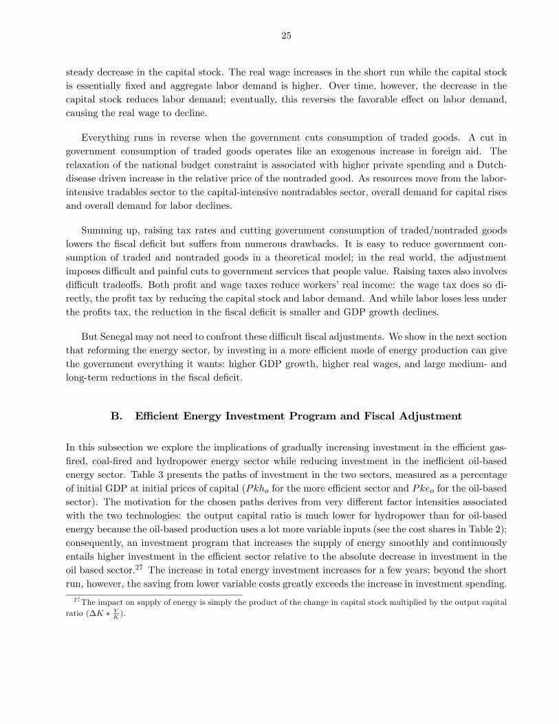
In this subsection we explore the implications of gradually increasing investment in the e¢ cient gas-�red, coal-�red and hydropower energy sector while reducing investment in the ine¢ cient oil-basedenergy sector. Table 3 presents the paths of investment in the two sectors, measured as a percentageof initial GDP at initial prices of capital (Pkho for the more e¢ cient sector and Pkeo for the oil-basedsector). The motivation for the chosen paths derives from very di¤erent factor intensities associatedwith the two technologies: the output capital ratio is much lower for hydropower than for oil-basedenergy because the oil-based production uses a lot more variable inputs (see the cost shares in Table 2);consequently, an investment program that increases the supply of energy smoothly and continuouslyentails higher investment in the e¢ cient sector relative to the absolute decrease in investment in theoil based sector.27 The increase in total energy investment increases for a few years; beyond the shortrun, however, the saving from lower variable costs greatly exceeds the increase in investment spending.

27The impact on supply of energy is simply the product of the change in capital stock multiplied by the output capitalratio (�K � Y

K).

26

Table 3. E¢ cient Energy Investment ProgramIne¢ cient sector (Ie) and more e¢ cient sector (Ih)

Year 1 2 3 4 5 6 7 8 9 10::: 15:: 20:::

Pkho�(Ih�Iho)yo

0 1:0 1:4 1:8 2:1 2:5 2:5 2:5 2:4 2:3 1:5 1:5

Pkeo�(Ie�Ieo)yo

0 �0:5 �0:5 �0:5 �0:5 �0:5 �0:5 �0:5 �0:5 �0:5 �0:5 �0:5

Note: Numbers are in percent of initial GDP (yo = 100)

Implementation of the energy investment program in Table 3 raises energy supply by 70 percent.Relaxing the energy bottleneck has positive e¤ects on real GDP and real wages, which increase 5percent and 2 percent, respectively (Figure 4). As the total supply of energy increases, the return one¢ cient energy investment declines. Shadow prices of household and �rm energy consumption alsodecline but stay above the o¢ cial price (excess demand and rationing persist). Private investmentand private capital stock fall in the short run and then recover slowly � the capital stock does notregain its pre-reform level until year 18. The �scal de�cit rises for 5 years, but then decreases rapidly,dropping to 4:5 percent of GDP at the end of the �rst decade.

The temporary decline in private investment stems from two e¤ects. First, the increase in publicinvestment in the energy sector drives up the supply price of capital by bidding up the prices of capitalinputs purchased from the nontradables sector (construction, for example). Second, the anticipationof higher income in the future leads the private sector to consume more today. Since income does notincrease in the short run, the counterpart of consumption smoothing is lower saving and a temporarydecrease in private investment.

As noted earlier, the temporary increase in �scal de�cit re�ects the fact that in the short runtotal spending on energy mirrors higher investment in the energy sector. The increase in investmentis driven, to repeat, by the di¤erence in factor intensities in the two energy sectors: production inthe ine¢ cient energy sector involves much higher recurrent costs (mainly oil), so the �scal gain fromreducing investment in that sector does not fully materialize at the outset. It materializes only afterdecreases in the capital stock bring about large reductions in expenditure on variable inputs (used in�xed coe¢ cient proportions with the capital stock). By contrast, in the e¢ cient energy sector recurrentcosts are labor costs, which are a very small part of total cost. Since the �scal cost of new investment inthe e¢ cient sector is roughly constant over time while the �scal saving from downsizing the ine¢ cientsector grows steadily, the reform program increases spending in the short run but generates large costssavings in the medium run. When the cost savings combine with higher tax revenue from greaterGDP growth and more revenue from energy sales, the total �scal gain rises to 3 percent of GDP inyear �fteen. When investment in the ine¢ cient energy sector is reduced and investment in the e¢ cientenergy sector is raised, the �scal gains occur more gradually overtime leading to a short term increasein de�cit. The �scal de�cit rises initially from about 6 to 6:8 percent of GDP and then it declines verystrongly to about 2 percent of GDP in the long run as you reap the bene�ts from lower cost and more

27

e¢ cient energy production, and expansion in output which brings in other tax revenues.

0 10 20 30

0

2

4

6

8

10Real Wage

0 10 20 30

­2

0

2

4

6

8Private Investment

0 10 20 30­0.5

0

0.5

1Private Capital

0 10 20 300

10

20

30

40

50

60

70Total Energy Output

0 10 20 300

2

4

6

8

10

12

Change in Real GDP

0 10 20 3010

15

20

25

30Return on Investment

Efficient Energy

0 10 20 300

1

2

3Shadow and Official Prices

HouseholdFirmsOfficial

0 10 20 302

3

4

5

6

7

8

9Deficit (% of GDP)

Figure 4: E¢ cient Energy Investment Program.Variables are expressed as percentage deviations fromthe initial steady state, unless otherwise indicated.

The large �scal gains that accrue over the medium run allow the government to consider broader-based, more pro-growth investment programs. We examine several scenarios of this type. In Figure 5the government initiates large increases in non-energy infrastructure investment once the �scal de�citdrops below its pre-reform level (Table 4). This program slows the reduction in the �scal de�citbut produces much larger gains in real income, real wages, and private investment. Real wages rise7 percent, while private investment and real GDP increase 6 percent and 10 percent, respectively.The corresponding numbers in Figure 4 are 2:4 percent, 2 percent, and 5:8 percent. Note also thatthe return on infrastructure investment does not fall nearly as much as the return on e¢ cient energyinvestment;28 even at year twenty, the return is well above 20 percent. This suggests that further gainscould be reaped by shifting more of the �scal savings from energy reform to non-energy infrastructureinvestment.28Because the percent increase in infrastructure investment is not as much as that of e¢ cient energy investment.

28

Table 4. E¢ cient Energy Program and Delayed Investment in other InfrastructureIne¢ cient sector (Ie), more e¢ cient sector (Ih), and other infrastructure (Iz)

Year 1 2 3 4 5 6 7 8 9 10::: 15:: 20:::

Pkho�(Ih�Iho)yo

0 1:0 1:4 1:8 2:1 2:5 2:5 2:5 2:4 2:3 1:5 1:5

Pkeo�(Ie�Ieo)yo

0 �0:5 �0:5 �0:5 �0:5 �0:5 �0:5 �0:5 �0:5 �0:5 �0:5 �0:5

Pzo�(Iz�Izo)yo

0 0 0 0 0 0 0 0 0:4 0:8 2:5 1:7

Note: Numbers are in percent of initial GDP (yo = 100)

Perhaps the most important result in Figure 5 is that the �scal cost of purchasing more growth isvery small. Although the permanent increase in non-energy infrastructure investment is 1:7 percentof initial GDP, the �scal de�cit in year twenty rises only :7 percent of GDP (3:2 percent in Figure 5vs. 2:5 percent in Figure 4). In general equilibrium, additional revenue from user fees and taxes payfor 60 percent of the extra investment.

We remind the reader that the runs in Figures 4 and 5 sidestep the issue of how to pay forthe temporary increase in total energy investment.29 If we reject the business-as-usual approach ofraising taxes or cutting public sector consumption, then the government is left with two choices: (i)temporarily raise o¢ cial energy prices or (ii) borrow more in the regional bond market or the Eurobondmarket. We examine these scenarios in the next three sections.

C. Temporarily Raising O¢ cial Energy Prices

Since user fees from energy consumption do not cover even recurrent costs, one can argue that bothhouseholds and �rms should pay higher prices to help �nance the broad-based energy + infrastructureinvestment program. This is done in Figure 6, where energy prices increase 35 percent for 4 years andthen drop back to their previous level. The temporary price increase fully covers the bill for higherinvestment until the cost saving and revenue gains from the reform kick in at year 6, after which the�scal de�cit decreases rapidly. The impact on real variables is similar to that in Figure 5, exceptprivate investment falls more in the short run as savers bear more of the tax burden when high energyprices replace cuts in transfer payments.30

29To get a solution, the runs assume that ransfer payments adjust to balance the budget. The change in transferpayments that balance the budget is then added to the initial �scal de�cit to track the time-varying �scal e¤ects of theprogram.30Transfers are proportional to each group�s share in total labor supply. In addition, the share of energy in total

consumption is 2.7 percent for saving households versus 0.4 percent for poor, non-saving households. Saving householdssmooth the e¤ects on consumption by cutting investment in the short-run. Hence investment cuts to smooth the pathof consumption are larger in the case of energy price increases.

29

0 10 20 30

0

2

4

6

8

10Real Wage

0 10 20 30

­2

0

2

4

6

8Private Investment

0 10 20 30­1

­0.5

0

0.5

1

1.5

2

2.5Private Capital

0 10 20 300

10

20

30

40

50

60

70Total Energy Output

0 10 20 300

2

4

6

8

10

12

Change in Real GDP

0 10 20 3010

15

20

25

30Return on Investment

Efficient EnergyInfrastructure

0 10 20 300

1

2

3Shadow and Official Prices

HouseholdFirmsOfficial

0 10 20 302

3

4

5

6

7

8

9Deficit (% of GDP)

Figure 5: E¢ cient Energy Program and Delayed Non-Energy Investment.Variables are ex-pressed as percentage deviations from the initial steady state, unless otherwise indicated.

It is hard to judge whether the price increases would be socially controversial. The public mightbe willing to pay more for a few years if it understands that higher prices are part of a package deal� that they pay for increases in the supply of energy that the public wants and values. But thisrationale might be a hard sell. Because existing energy production is so ine¢ cient, energy prices arealready very high in Senegal. Raising them further is unlikely to prove popular.

D. Temporary Borrowing in the Regional Bond Market

The natural alternative to raising energy prices is to borrow against future �scal gains to �nancethe temporary increase in the �scal de�cit. One possibility is to issue CFA franc bonds in the re-gional market comprised by countries belonging to the West African Economic and Monetary Union(WAEMU).31

31When Senegal issues CFA Franc denominated bond, holders can be Senegal residents as well as individuals andcommercial banks in the remaining parts of the WAEMU region. In 2012, CFA franc denominated debt was composedof 40 percent domestic (i.e. Senegal residents) and 60 percent regional (i.e. WAEMU region�s residents excluding

30

0 10 20 30

0

2

4

6

8

10Real Wage

0 10 20 30

­2

0

2

4

6

8Private Investment

0 10 20 30­1.5

­1

­0.5

0

0.5

1

1.5

2Private Capital

0 10 20 300

10

20

30

40

50

60

70Total Energy Output

0 10 20 300

2

4

6

8

10

12

Change in Real GDP

0 10 20 3010

15

20

25

30Return on Investment

Efficient EnergyInfrastructure

0 10 20 300

1

2

3Shadow and Official Prices

HouseholdFirmsOfficial

0 10 20 302

3

4

5

6

7

8

9Deficit (% of GDP)

Figure 6: E¢ cient Energy Program and Delayed Non-Energy Investment: Raising EnergyPrices.Variables are expressed as percentage deviations from the initial steady state, unless otherwise indicated.

Regional borrowing requires temporary supporting �scal adjustment to prevent explosive growthin the public debt. In Figure 7 the cut in transfer payments is limited to :5 percent of initial GDP.Aided by this small amount of �scal support, the scheme works very well. The paths for the realwage, real GDP, and private investment are broadly similar to those in Figure 6. Domestic (total)debt increases only slightly, rising from 12 (45) percent to 15 (48) percent of GDP. As expected, thesale of more debt increases the real interest rate. But the increase is small and short-lived. Afterrising to 3:64 in year 6, the interest rate declines continuously; in the long run, the rate decreases to3:1 percent .

The program with delayed infrastructure investment and temporary borrowing is safe and e¤ective.Arguably, however, it is too safe. Given the large �scal gains that energy reform delivers in the mediumrun, Senegal may wish to consider more aggressive pro-growth programs that frontload increases ininfrastructure investment.

Senegalese).

31

0 10 20 30

0

2

4

6

8

10Real Wage

0 10 20 30

­2

0

2

4

6

8Private Investment

0 10 20 300

2

4

6

8

10

12

Change in Real GDP

0 10 20 3010

15

20

25

30

35

40Return on Investment

Efficient EnergyInfrastructure

0 10 20 30­3

­2

­1

0

1

2

3

4Change in Transfers

0 10 20 302

3

4

5

6

7

8

9Deficit (% of GDP)

0 10 20 300

0.5

1

1.5

2

2.5

3Shadow and Official Prices

HouseholdFirmsOfficial

0 10 20 300

10

20

30

40

50

60

70Public Debt (% of GDP)

TotalDomestic

0 10 20 303

3.5

4

4.5

5Real Interest Rate

Figure 7: E¢ cient Energy Program and Delayed Non-Energy Investment: Regional Bor-rowing.Variables are expressed as percentage deviations from the initial steady state, unless otherwise indi-

cated.

E. Pushing Harder for Growth: Frontloaded Infrastructure Investment andAggressive Borrowing in the Regional versus Eurobond Market

Figure 8 shows the outcome when the government increases infrastructure concurrently with theenergy reform program. Infrastructure investment rises by 0:4-0:5 percent of GDP until the cumulativeincrease reaches 2:1 percent of initial GDP in year 6 (Table 5). By year 15, the stock of infrastructurehas increased 17 percent vs. 11 percent in the runs with delayed infrastructure investment.

32

Table 5. E¢ cient Energy Program and Frontloaded Investment in other InfrastructureIne¢ cient sector (Ie), more e¢ cient sector (Ih), and other infrastructure (Iz)

Year 1 2 3 4 5 6 7 8 9 10::: 15:: 20:::

Pkho�(Ih�Iho)yo

0 1:0 1:4 1:8 2:1 2:5 2:5 2:5 2:4 2:3 1:5 1:5

Pkeo�(Ie�Ieo)yo

0 �0:5 �0:5 �0:5 �0:5 �0:5 �0:5 �0:5 �0:5 �0:5 �0:5 �0:5

Pzo�(Iz�Izo)yo

0 0:4 0:8 1:3 1:7 2:1 2:1 2:1 2:1 2:1 2:1 2:1

Note: Numbers are in percent of initial GDP (yo = 100)

Frontloading generates signi�cant additional bene�ts. In contrast to the runs with delayed in-frastructure investment, there is very little crowding out of of private investment in the short run.This together with faster growth in the stock of infrastructure add 2-3 percentage points to the in-creases in the real wage, private investment, and real income at the 10- and 20-year horizons.

Senegal pays a price for these gains. Ramping up infrastructure investment right away requiresmuch more borrowing. Domestic debt rises to nearly 30 percent of GDP, while total debt peaks at 60percent in year 11. There is also an adverse e¤ect on the country�s �nancial terms of trade. BecauseSenegal is big in the regional bond market, the extra borrowing pushes the real interest rate up from3:5 percent to 4:5 percent. The marginal cost of debt is thus several percentage points higher thanthe average cost.

In Figure 9, the government taps the Eurobond market instead of the WAEMU market. Theinterest rate on domestic debt rises much less, but since Eurobond debt carries a yield of 7:5 percentthe overall cost of borrowing rises.32 This shows up in a longer period of depressed transfer payments(20 years in Figure 9 vs. 17 years in Figure 8). Eurobond borrowing is competitive with borrowing inthe regional only if the government is anxious to tie down the interest rate.33

32The interest rate rises in the regional market because the private sector borrows more to �nance temporary dissaving.33These results point to regional borrowing being supperior to Eurobond issuance. In 2012, real yields on Eurobonds

hovered around 7.5 percent while that on the Regional bond was about 3.5 percent. Regional borrowing may involverollover risks but it is not clear as to which way these risks could go. Recently, the yield on the Eurobond has decline inlight of macroeconomic developments in the OECD countries. However this decline (although it may call for locking-inlower rates now) may not last long because we may see a reversal once the Federal Reserve Board begins tapering o¤.One of the bene�ts of relying on the regional bond market is that it may help deepen the �nancial sector in the region.In our analysis we assume that regional borrowing is less expensive relative to Eurobond borrowing because the ratedi¤erential in 2012. We are aware that the costs and bene�ts of each �nancing method are open to discussion.

33

0 10 20 30

0

2

4

6

8

10Real Wage

0 10 20 30

­2

0

2

4

6

8Private Investment

0 10 20 300

2

4

6

8

10

12

Change in Real GDP

0 10 20 3010

15

20

25

30

35

40Return on Investment

Efficient EnergyInfrastructure

0 10 20 30­3

­2

­1

0

1

2

3

4Change in Transfers

0 10 20 302

3

4

5

6

7

8

9Deficit (% of GDP)

0 10 20 300

0.5

1

1.5

2

2.5

3Shadow and Official Prices

HouseholdFirmsOfficial

0 10 20 300

10

20

30

40

50

60

70Public Debt (% of GDP)

TotalDomestic

0 10 20 303

3.5

4

4.5

5Real Interest Rate

Figure 8: E¢ cient Energy and Frontloaded Non-Energy Investment: Regional Borrow-ing.Variables are expressed as percentage deviations from the initial steady state, unless otherwise indicated.

34

0 10 20 30

0

2

4

6

8

10Real Wage

0 10 20 30

­2

0

2

4

6

8Private Investment

0 10 20 300

2

4

6

8

10

12

Change in Real GDP

0 10 20 3010

15

20

25

30

35

40Return on Investment

Efficient EnergyInfrastructure

0 10 20 30­3

­2

­1

0

1

2

3

4Change in Transfers

0 10 20 302

3

4

5

6

7

8

9Deficit (% of GDP)

0 10 20 300

0.5

1

1.5

2

2.5

3Shadow and Official Prices

HouseholdFirmsOfficial

0 10 20 300

10

20

30

40

50

60

70Public Debt (% of GDP)

TotalEurobond

0 10 20 303

3.5

4

4.5

5Real Interest Rate

Figure 9: E¢ cient Energy and Frontloaded Non-Energy Investment: Eurobond Borrow-ing.Variables are expressed as percentage deviations from the initial steady state, unless otherwise indicated.

35

VI. Concluding Remarks

Senegal needs to reform its ailing oil-based energy sector in order to lower costs and increase thesupply of energy. Di¢ culties in the existing ine¢ cient mode of energy production have slowed growthand contributed signi�cantly to rising �scal de�cits and rapid growth of the public debt since 2006.

To analyze the impacts of di¤erent adjustment programs on growth, private investment, realwages, debt and the �scal de�cit, we use a variant of the two-sector, open-economy dynamic generalequilibrium model developed by Bu¢ e et al. (2012). This model incorporates sector-speci�c capi-tal, productivity-enhancing infrastructure, external concessional and commercial debt, a consumptionvalue added tax and government transfers payments, variable e¢ ciency of public investment, an ab-sorptive capacity constraint, and non-savers consumers. We adapted the model for Senegal by addingwage and pro�t taxes, government consumption of traded and nontraded goods, controlled energyprices, regional and domestic currency debt, an ine¢ cient, oil-based energy sector, and a new, low-cost gas, coal and hydropower energy sector. After calibrating the model for Senegal, we investigatedthe e¤ects of varying traditional �scal policy instruments one at time before focusing on policy pack-ages that increase public investment in energy and infrastructure in scenarios with varying degrees ofdebt �nance and with di¤erent types of supporting �scal adjustment.

Raising taxes and cutting expenditure lowers the �scal de�cit at all horizons. Traditional �scaladjustment involves di¢ cult tradeo¤s, however. Higher wage and pro�t taxes reduce workers� realincome, while cuts in government consumption reduce the supply of public services; the pro�t tax alsolowers the capital stock and real GDP.

Reforming the energy sector is the best way to adjust. An energy program that invests in a new,low-cost coal-�red and hydropower energy sector while downsizing the ine¢ cient oil-based sector cangive the government everything it wants: higher GDP growth, higher real wages, and large medium-and long-term reductions in �scal de�cits. Real GDP and real wages increase even more when some ofthe �scal gains from the energy reform program are used to �nance delayed investments in non-energyinfrastructure. The only potential drawback is that the �scal de�cit increases in the short run. Thetemporary increase in the �scal de�cit is easily managed, however, by borrowing in the regional bondmarket.

Given the large �scal gains that result from implementation of the e¢ cient energy investmentprogram, the government should cautiously give serious consideration to a �big-push�program thatimmediately supplements higher energy investments with a substantial increase in infrastructure in-vestment. Our analysis argues that the bene�ts of a big push outweigh its costs. The program, whenunderpinned by an e¢ cient public investment process, generates signi�cant additional gains in realGDP, real wages, and private investment. The public debt grows rapidly for a few years, but in themedium run the government reaps a large �scal dividend on the order of three percent of GDP.

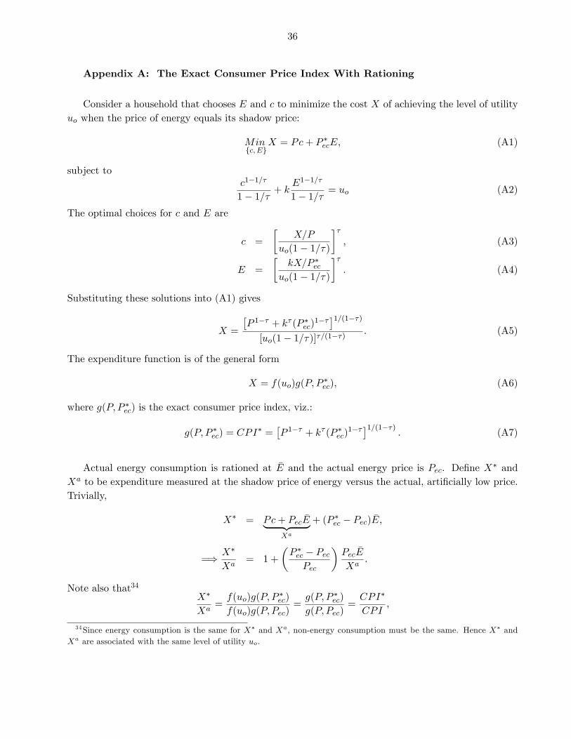
36

Appendix A: The Exact Consumer Price Index With Rationing

Consider a household that chooses E and c to minimize the cost X of achieving the level of utilityuo when the price of energy equals its shadow price:

Minfc; Eg

X = Pc+ P �ecE; (A1)

subject toc1�1=�

1� 1=� + kE1�1=�

1� 1=� = uo (A2)

The optimal choices for c and E are

c =

�X=P

uo(1� 1=�)

��; (A3)

E =

�kX=P �ec

uo(1� 1=�)

��: (A4)

Substituting these solutions into (A1) gives

X =

�P 1�� + k� (P �ec)

1�� �1=(1��)[uo(1� 1=�)]�=(1��)

: (A5)

The expenditure function is of the general form

X = f(uo)g(P; P�ec); (A6)

where g(P; P �ec) is the exact consumer price index, viz.:

g(P; P �ec) = CPI� =�P 1�� + k� (P �ec)

1�� �1=(1��) : (A7)

Actual energy consumption is rationed at �E and the actual energy price is Pec. De�ne X� andXa to be expenditure measured at the shadow price of energy versus the actual, arti�cially low price.Trivially,

X� = Pc+ Pec �E| {z }Xa

+ (P �ec � Pec) �E;

=) X�

Xa= 1 +

�P �ec � Pec

Pec

�Pec �E

Xa:

Note also that34X�

Xa=f(uo)g(P; P

�ec)

f(uo)g(P; Pec)=g(P; P �ec)

g(P; Pec)=CPI�

CPI;

34Since energy consumption is the same for X� and Xa, non-energy consumption must be the same. Hence X� andXa are associated with the same level of utility uo.

37

where CPI is the exact consumer price index associated with the rationed level of consumption. Itfollows that

CPI�

CPI= 1 +

�P �ec � Pec

Pec

�Pec �E

Xa;

=) CPI =CPI�

1 + e(P�ec � Pec)=Pec

; (A8)

where e = Pec �E=Xa is the consumption share of energy measured at the o¢ cial price Pec.

38

Appendix B: Policy Reaction Functions and the Path of Government Debt

The government budget constraint is

bt � bt�1 = Pz;t

"�1 +

iz;t~zt�1

� � � g��(iz;t � iz;o) + iz;o

#+ Pke;tie;t + Pkh;tih;t

+Pn;tgn;t + Pm;tgm;t +rd � g1 + g

dt�1 +rdc � g1 + g

dct�1 +rt�1 � g1 + g

bt�1 + Tt + wt(Le;t + Lh;t)

+Po;tOt + Pf;tqf;t � Pec;t( �Es;t + E1;t)� Pe;t(Ex;t + En;t)� htPt(cs;t + c1;t)� xt � �tzt�1�hw;twtL(1 + a)� hp;t[Pxqx;t + Pn;tqn;t � Pe;t(En;t + Ex;t)� wt(Lx;t + Ln;t)]: (B1)

In the short run, the de�cit can be �nanced by issuing more debt. Eventually, however, some subsetof policy variables must adjust to cover the ex ante �nancing gap. The latter is the size of the revenueshortfall when T , h, hw, hp, gn, and gm in (B1) equal their initial values:

GAPt = Pz;t

"�1 +

iz;t~zt�1

� � � g��(iz;t � iz;o) + iz;o

#+ Pke;tie;t + Pkh;tih;t

+Pn;tgn;o + Pm;tgm;o +rd � g1 + g

dt�1 +rdc � g1 + g

dct�1 +rt�1 � g1 + g

bt�1 + To + wt(Le;t + Lh;t)

+Po;tOt + Pf;tqf;t � Pec;t( �Es;t + E1;t)� Pe;t(Ex;t + En;t)� hoPt(cs;t + c1;t)� xt � �tzt�1�hw;owtL(1 + a)� hp;o[Pxqx;t + Pn;tqn;t � Pe;t(En;t + Ex;t)� wt(Lx;t + Ln;t)]: (B2)

Policy makers specify the share of �scal adjustment borne by each policy variable. This determinesthe long-run target values of the adjusting variables. For example, if transfers and government con-sumption of traded goods adjust, then

Ttarget,t = To � �GAPt; 0 � � � 1; (B3)

gm, target,t = gm;o � (1� �)GAPtPm;t

; 0 � � � 1: (B4)

Equations (B3) and (B4) are paired with a target for the long-run level of government debt. Thereaction functions that govern the paths of h and gm incorporate these targets as well as socio-politicalconstraints on how much and how fast �scal policy can change:

gm;t = Max fgm;t�1 + �1(gm, target,t � gm;t�1) + �2(bt�1 � btarget); �gmg ; (B5)

Tt = Max�Tt�1 + �3(Ttarget,t � Tt�1)� �4(bt�1 � btarget); �T

: (B6)

�gm and and �T are lower bounds on gm and T . Inside the bounds, the parameters �1-�4 determinewhether policy adjustment is fast or slow. Under "slow" adjustment, the debt instrument that variesendogenously to satisfy the government budget constraint may rise above its target level in the timeit takes gm and T to reach gm, target and Ttarget. When this happens, the transition path includes aphase in which T < Ttarget and gm < gm, target to generate the �scal surpluses needed to pay down thedebt.

39

References

Adam, C. and D. Bevan, 2006, �Aid and the Supply Side: Public Investment, Export Performance, and DutchDisease in Low-Income Countries,� The World Bank Economic Review, Vol. 20(2), pp. 261-290.

Agenor, R. and P. Montiel, 1999, Development Macroeconomics, 2nd edition (Princeton, N.J.; Princeton Uni-versity Press).

Agenor, R., 2010, �A Theory of Infrastructure-Led Development,�Journal of Economics Dynamics and Control,Vol. 34(5), pp. 932-950.

Andrle, M., A. David, R. Espinoza, M. Mills, and L.F. Zanna, 2012, �As You Sow So Shall You Reap: PublicInvestment Surges, Growth, and Debt Sustainability in Togo,�IMF Working Paper, forthcoming.

Aresto¤, F. and C. Hurlin (2006), �Estimates of Government Net Capital Stocks for 26 Developing Countries,1970-2002,�World Bank Policy Research Working Paper 3858.

Arslanalp, Serkan Fabian Bornhorst, Sanjeev Gupta, and Elsa Sze, 2010, �Public Capital and Growth�, IMFWorking Paper 10/175 (Washington: International Monetary Fund).

Arnone, M. and A. Presbitero, 2010, Debt Relief Initiatives: Policy Design and Outcomes, forthcoming (Ash-gate).

Arrow, K., 1962, �The Economic Implications of Learning by Doing.�Review of Economic Studies 29, 153-173.

Asea, P. and C. Reinhart, 1996, �Le Prix de l�Argent: How (Not) to Deal with Capital Flows.� Journal ofAfrican Economies 5 (AERC Supplement), 231-272.

Barkbu, B., C. Beddies, and M. Le Manchec, 2008, �The Debt Sustainability Framework for Low-IncomeCountries.�IMF Occasional Paper, No. 266.

Barro, R., 1990, �Government Spending in a Simple Model of Endogenous Growth,�Journal of Political Econ-omy, Vol. 98(5), pp. S103-26.

Barro, R. and X. Sala-i-Martin, 1992, �Public Finance in Models of Economic Growth,�Review of EconomicStudies, Vol. 59(4), pp. 645-61.

Berg, A., T. Mirzoev, R. Portillo, and L.F. Zanna, 2010a, �The Short-Run Macroeconomics of Aid In�ows:Understanding the Interaction of Fiscal and Reserve Policy,�IMF Working Paper 10/65.

Berg, A., J. Gottschalk, R. Portillo, and L.F. Zanna, 2010b, �The Macroeconomics of Medium-Term AidScaling-Up Scenarios.�IMF Working Paper 10/160.

Berg, A., R. Portillo, S. Yang, and L.F. Zanna, 2012, �Public Investment in Resource Abundant Low-IncomeCountries,�IMF Working Paper, forthcoming .

Blundell, R., 1988, �Consumer Behavior: Theory and Evidence � A Survey.�Economic Journal 98, 16-65.

Blundell, R., P. Pashardes, and G. Weber, 1993, �What do we Learn about Consumer Demand Patterns fromMicro Data?�American Economic Review 83, 570-597.

Briceño-Garmendia, C., K. Smits, and V. Foster, 2008, �Financing Public Infrastructure in Sub-Saharan Africa:Patterns and Emerging Issues.�AICD Background Paper 15 (World Bank).

Bohn, H., 1998, �The Behavior of US Public Debt and De�cits,�Quarterly Journal of Economics, Vol 113(3),pp. 949-963.

Bu¢ e, E. F.,A. Berg, C. A. Pattillo, R. Portillo, and L-F. Zanna, 2012, �Public Investment, Growth, and DebtSustainability: Putting Together the Pieces,�IMF Working Paper 12/144.

40

Calderón, C., E. Moral-Benito, and L. Servén, 2009, �Is Infrastructure Capital Productive? A Dynamic Het-erogeneous Approach.�Mimeo (World Bank).

Calderón, C. and L. Servén, 2010, �Infrastructure in Latin America.�Policy Research Working Paper, No. 5317(World Bank).

Chatterjee, S. and S. Turnovsky, 2007, �Foreign Aid and Economic Growth: The Role of Flexible Labor Supply,�Journal of Development Economics, Vol. 84(1), pp. 507�533.

Celasun, O., X. Debrun, and J. D. Ostry, 2007, �Primary Surplus Behavior and Risks to Fiscal Sustainabilityin Emerging Market Countries: A �Fan-Chart�Approach,�IMF Sta¤ Papers, Vol. 53(3), pp. 401-425.

Cerra, V., S. Tekin, and S. Turnovsky, 2008, �Foreign Aid and Real Exchange Rate Adjustments in a FinanciallyConstrained Dependent Economy,�IMF Working Paper 08/204.

Clinton, K., R. Garcia-Saltos, M. Johnson, O. Kamenik, and D. Laxton, 2010, �International De�ation Risksunder Alternative Macroeconomic Policies,� Journal of the Japanese and International Economies, Vol.24(2), pp. 140-177.

Collier, P., 2007, �The Bottom Billion: Why the Poorest Countries are Failing and What Can Be Done AboutIt,�Oxford University Press, New York.

Cowan, D., 2010, �Sub-Saharan Africa Macro View.�Citigroup Global Markets.

Dabla-Norris, E., J. Brumby, C. Papageorgiou, A. Kyobe, and Z. Mills, 2011, �Investing in Public Investment:An Index of Public Investment Management Quality,�IMF Working Paper, 11/37.

Dagher, J., J. Gottschalk, and R. Portillo, 2012, �The Short-run Impact of Oil Windfalls in Low-income Coun-tries: A DSGE Approach.�Journal of African Economies, forthcoming.

Dalgaard, C. and H. Hansen, 2005, �The Return to Foreign Aid.� Discussion Paper No. 05-04, Institute ofEconomics, University of Copenhagen.

Deaton, A., and D. Muellbauer, 1980, Economics and Consumer Behavior (New York, Cambridge UniversityPress).

Eaton, J., 2002, �The HIPC Initiative: The Goals, Additionality, Eligibility, and Debt Sustainability.�Mimeo(Operations Evaluation Department, World Bank).

Eberhard, A., V. Foster, C. Bricendo-Garmendia, F. Ouedraogo, D. Camos, and M. Shkaratan, 2008, �Un-derpowered: The State of the Power Sector in Sub-Saharan Africa.� AICD Background Paper 6 (WorldBank).

Escribano, A., J. Guasch, and J. Pena, 2008, �Impact of Infrastructure Constraints on Firm Productivity inAfrica.�AICD Working Paper No. 9 (World Bank).

EURODAD, 2001, �Putting Poverty Reduction First.�(European Network on Debt and Development)

EURODAD, 2009, �Review of the DSF: Bank & Fund Declare Countries Can Borrow More.�(European Networkon Debt and Development)

Fedelino, A. and A. Kudina, 2003, �Fiscal Sustainability in African HIPC Countries: A Policy Dilemma?�IMFWorking Paper, No. 03/187.

Fernández-Villaverde, J., P. Guerrón-Quintana, J. Rubio-Ramírez, and M. Uribe, 2011. �Risk Matters: TheReal E¤ects of Volatility Shocks,�American Economic Review, Vol. 101(6), pp. 2530-2561.

Foster, V. and C. Briceño-Garmendia, 2010, Africa�s Infrastructure: A Time for Transformation, forthcoming(Agence Francaise de Developpement and the World Bank).

41

Futagami, K., Y. Morita, and A. Shibata, 1993, �Dynamic Analysis of an Endogenous Growth Model withPublic Capital,�Scandinavian Journal of Economics, Vol. 95(4), pp. 607-25.

Garcia, M. and R. Rigobon, 2005, �A Risk Management Approach to Emerging Market�s Sovereign Debt Sustain-ability with an Application to Brazilian Data,� in In�ation Targeting, Debt, and the Brazilian Experience:1999 to 2003, editors, Francesco Giavazzi, Ilan Goldfajn, and Santiago Herrera, MIT Press.

Ghosh, A., J. Kim, E. Mendoza, J. D. Ostry, and M. Qureshi, 2011. �Fiscal Fatigue, Fiscal Space and DebtSustainability in Advanced Economies,�NBER Working Papers 16782, National Bureau of Economic Re-search.

Glomm, Gerhard and B. Ravikumar, 1994, �Public investment in infrastructure in a simple growth model,�Journal of Economic Dynamics and Control, Vol. 18(6), pp. 1173-1187.

Gongalez, G. and H. Sala, 2011, �The Frisch Elasticity in Mercosur Countries: A Pseudo-Panel Approach,�Institute for the Study of Labor (IZA) Discussion Paper, No. 5993.

Greiner, A., 2007, �An Endogenous Growth Model with Public Capital and Sustainable Government Debt,�The Japanese Economic Review, Vol. 58(3), pp. 345-361.

Greiner, A., W. Semmler, and G. Gong, 2005, The Forces of Economic Growth: A Time Series Perspective, 1st

edition (Princeton, N.J.; Princeton University Press).

Gueye, C. and A. Sy, 2010, �Beyond Aid: How Much Should African Countries Pay to Borrow?�IMF WorkingPaper, No. 10/140.

Gupta, S., R. Powell, and Y. Yang, 2006, Macroeconomic Challenges of Scaling Up Aid to Africa: A Checklistfor Practitioners (International Monetary Fund).

Hjertholm, P., 2003, �Theoretical and Empirical Foundations of HIPC Debt Sustainability Targets.�Journal ofDevelopment Studies 39, 67-100.

Hulten, C., 1996, �Infrastructure Capital and Economic Growth: How Well You Use It May Be More ImportantThan How Much You Have.�NBER Working Paper, No. 5847.

Hulten, C., E. Bennathan, and S. Srinivasan, 2006, �Infrastructure, Externalities, and Economic Development:A Study of Indian Manufacturing.�World Bank Economic Review 20, xx-xx.

International Monetary Fund, 2007a, �Regional Economic Outlook: Sub-Saharan Africa,�SM/07/319, availableat http://www.imf.org/external/pubs/ft/reo/2007/afr/eng/sreo1007.pdf

International Monetary Fund, 2007b, �Ghana: Sta¤ Report for the 2007 Article IV Consultation,�SM/07/156,available at http://www.imf.org/external/pubs/ft/scr/2007/cr07210.pdf

International Monetary Fund, 2009a, �Changing Patterns in Low-Income Country Financing andImplications for Fund Policies on External Financing and Debt,� SM/09/56, available athttp://www.imf.org/external/np/pp/eng/2009/022509a.pdf

International Monetary Fund, 2009b, �Debt Limits in Fund-Supported Programs: Proposed New Guidelines�,SM/09/215, available at http://www.imf.org/external/np/pp/eng/2009/080509.pdf

International Monetary Fund, 2010, �Sta¤ Guidance Note on the Application of the Joint Fund-Bank Debt Sustainability Framework for Low-Income Countries,� SM/10/16, available athttp://www.imf.org/external/np/pp/eng/2010/012210.pdf

International Monetary Fund and World Bank, 2006, �Applying the Debt SustainablityFramework for Low-Income Countries: Post-Debt Relief,� SM/06/364, available athttp://www.imf.org/external/np/pp/eng/2006/110606.pdf

42

International Monetary Fund and World Bank, 2009, �A Review of Some Aspects ofthe Low-Income Country Debt Sustainability Framework,� SM/09/216, available athttp://www.imf.org/external/np/pp/eng/2009/080509a.pdf

International Monetary Fund and World Bank, 2010, �Preserving Debt Sustainability inLow-Income Countries in the Wake of the Global Crisis,� SM/10/76 , available athttp://www.imf.org/external/np/pp/eng/2009/080509a.pdf

Isham, Jonathan and Daniel Kaufmann, 1999, �The Forgotten Rationale For Policy Reform: The Productivityof Investment Projects�Quarterly Journal of Economics, February, Vol. 114, No. 1, pp. 149�184.

Keane, M. P., and R. Rogerson, 2011, �Reconciling Micro and Macro Labor Supply Elasticities: A StructuralPerspective,�NBER Working Paper, No. 17430.

Kose, M. A., and R. Riezman, 2001, �Trade Shocks and Macroeconomic Fluctuations in Africa,� Journal ofDevelopment Economics, Vol. 65(1), pp. 55-80.

Kraay, A. and V. Nehru, 2006, �When Is External Debt Sustainable?,�World Bank Economic Review, Vol.20(3), pp. 341-365.

Lluch, C., A. Powell, and R. Williams, 1977, Patterns in Household Demand and Saving (London, OxfordUniversity Press).

Mendoza, E. and M. Oviedo, 2004, �Public Debt, Fiscal Solvency and Macroeconomic Uncertainty in LatinAmerica: The Cases of Brazil, Colombia, Costa Rica, and Mexico,�NBER Working Papers 10637, NationalBureau of Economic Research.

Neumeyer, P., and F. Perri, 2005, �Business Cycles in Emerging Economies: the Role of Interest Rates,�Journalof Monetary Economics, Vol. 52(2), pp. 345-380.

Ogaki, M., J. Ostry, and C. Reinhart, 1996, �Saving Behavior in Low- and Middle-Income Developing Countries.�IMF Sta¤ Papers 43, 38-71.

Panizza, U., 2008, �Domestic and External Public Debt in Developing Countries.�UNCTAD Discussion Paper,No. 188.

Perrault, J., L. Savard, and A. Estache, 2010, �The Impact of Infrastructure Spending in Sub-Saharan Africa:A CGE Modeling Approach.�Policy Research Working Paper, No. 5386 (World Bank).

Pritchett, L., 2000, �The Tyranny of Concepts: CUDIE (Cumulated, Depreciated, Investment E¤ort) is NotCapital.�Journal of Economic Growth 5, 361-384.

Raddatz, C., 2007, �Are External Shocks Responsible for the Instability of Output in Low-Income Countries?,�Journal of Development Economics, Vol. 84(1), pp. 155-187.

Redifer, L., 2010, �New Financing Sources for Africa�s Infrastructure De�cit.�IMF Survey Magazine: Countriesand Regions.

Sachs, J., 2002, �Resolving the Debt Crisis of Low-Income Countries.�Brookings Papers on Economic Activity1, 257-286.

Schmitt-Grohé, S. and M. Uribe, 2003, �Closing Small Open Economy Models,�Journal of International Eco-nomics, Vol. 61(1), pp. 163�185.

Servén, Luis, 2010, �Infrastructure investment and growth�, World Bank, in progress; presentation available athttp://www.imf.org/external/np/seminars/eng/2010/spr/lic/index.htm

Steadman Group (2009), �Financial Access Survey for Financial Sector Deepening,�Presentation.

43

Straub, S., 2008, �Infrastructure and Growth in Developing Countries: Recent Advances and Research Chal-lenges.�Policy Research Working Paper, No. 4460 (World Bank).

Thurlow, J., D. Evans, and S. Robinson, 2004, �A 2001 Social Accounting Matrix for Zambia.� InternationalFood Policy Research Institute (Washington, D.C.)

Thurlow, J., X. Diao, and C. McCool, 2008, �2004 Social Accounting Matrix: Malawi.� International FoodPolicy Research Institute.

Torres, C., C. M. Briceno-Garmendia, and C. Dominguez, 2011, �Senegal�s Infrastructure: A continental Per-spective.�Policy Research Working Paper, No. 5817 (World Bank).

Turnovsky, S., 1999, Methods of Macroeconomic Dynamics, 2nd edition (Cambridge, Mass.; MIT Press).

Uribe, M. and V. Yue, 2006, �Country Spreads and Emerging Countries: Who Drives Whom?,� Journal ofInternational Economics, Vol. 69(1), pp. 6-36.

UNCTAD, 2004, �Analysis of Eligibility and Debt Sustainability Criteria of the HIPC Initiative.�Chapter 2 inDebt Sustainablility: Oasis or Mirage? (United Nations Conference on Trade and Development).

van der Ploeg, F. and A. Venables, 2011, �Harnessing Windfall Revenues: Optimal Policies for Resource-RichDeveloping Economies,�Economic Journal, Vol. 121(551), pp. 1-30.

Wyplosz, C., 2007, �Debt Sustainability Assessment: The IMF Approach and Alternatives.� HEI WorkingPaper, No. 03/2007 (Graduate Institute of International Studies, Geneva).