EFFICIENT DISCRETIZATION OF LAPLACE …bremer/papers/polygonal.pdfEFFICIENT DISCRETIZATION OF LAPLACE BOUNDARY INTEGRAL EQUATIONS ON POLYGONAL DOMAINS3 of domains for which universal

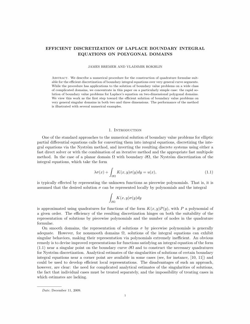
EFFICIENT DISCRETIZATION OF LAPLACE BOUNDARY INTEGRALEQUATIONS ON POLYGONAL DOMAINS

JAMES BREMER AND VLADIMIR ROKHLIN

Abstract. We describe a numerical procedure for the construction of quadrature formulae suit-

able for the efficient discretization of boundary integral equations over very general curve segments.While the procedure has applications to the solution of boundary value problems on a wide class

of complicated domains, we concentrate in this paper on a particularly simple case: the rapid so-

lution of boundary value problems for Laplace’s equation on two-dimensional polygonal domains.We view this work as the first step toward the efficient solution of boundary value problems on

very general singular domains in both two and three dimensions. The performance of the method

is illustrated with several numerical examples.

1. Introduction

One of the standard approaches to the numerical solution of boundary value problems for ellipticpartial differential equations calls for converting them into integral equations, discretizing the inte-gral equations via the Nystrom method, and inverting the resulting discrete systems using either afast direct solver or with the combination of an iterative method and the appropriate fast multipolemethod. In the case of a planar domain Ω with boundary ∂Ω, the Nystrom discretization of theintegral equations, which take the form

λσ(x) +∫∂Ω

K(x, y)σ(y)dy = u(x), (1.1)

is typically effected by representing the unknown functions as piecewise polynomials. That is, it isassumed that the desired solution σ can be represented locally by polynomials and the integral∫

∂Ω

K(x, y)σ(y)dy

is approximated using quadratures for functions of the form K(x, y)P (y), with P a polynomial ofa given order. The efficiency of the resulting discretization hinges on both the suitability of therepresentation of solutions by piecewise polynomials and the number of nodes in the quadratureformulae.

On smooth domains, the representation of solutions σ by piecewise polynomials is generallyadequate. However, for nonsmooth domains Ω, solutions of the integral equations can exhibitsingular behaviors, making their representation via polynomials extremely inefficient. An obviousremedy is to devise improved representations for functions satisfying an integral equation of the form(1.1) near a singular point on the boundary curve ∂Ω and to construct the necessary quadraturesfor Nystrom discretization. Analytical estimates of the singularities of solutions of certain boundaryintegral equations near a corner point are available in some cases (see, for instance, [10, 11]) andcould be used to develop efficient local representations. The disadvantages of such an approach,however, are clear: the need for complicated analytical estimates of the singularities of solutions,the fact that individual cases must be treated separately, and the impossibility of treating cases inwhich estimates are lacking.

Date: December 11, 2009.

1

2 JAMES BREMER AND VLADIMIR ROKHLIN

In this paper, we describe a numerical procedure for the construction of an orthonormal basis offunctions spanning the space of restrictions of functions σ satisfying a boundary integral equation

λσ(x) +∫

Γ

K(x, y)σ(y)dy = u(x) (1.2)

on a contour Γ to a small curve segment Γ0 ∈ Γ. The resulting basis can be used to form quadraturerules for the Nystrom discretization of the boundary integral equation (1.2) over Γ0 with the numberof quadratures nodes depending only on the rank of the basis. In other words, given a particularcurve segment Γ0, it is possible to construct numerically an efficient “purpose-made” quadraturefor the discretization of a boundary integral equation over Γ0. The principal step of the procedureconsists of computing solutions of the restriction of the integral equation (1.2) to the curve segmentΓ0 for a small collection of right-hand-sides. In effect, the problem of efficiently discretizing anintegral equation over a complex curve segment is reduced to the problem of solving the integralequation locally on that curve segment.

This procedure allows for a divide-and-conquer approach to the solution of boundary integralequations on complicated domains. For instance, given a domain Ω with boundary ∂Ω containingcorner points x1, . . . , xn, the procedure of this paper can be used to construct a collection of n effi-cient quadrature formulae, one for the discretization of ∂Ω near each corner point xn. The resultingquadrature formulae can then be used to produce what amounts to a compressed representation ofthe integral equation over the entire contour ∂Ω. This has obvious applications to parallelizationand in environments where the cost of inverting an integral equation that has been discretized as ann×n linear system is asymptotically greater than O(n). It is also a viable approach to the solutionof a problem too large to fit in available memory. This last application is expected to be importantin the case of boundary value problems on complicated surfaces in three dimensions.

A particularly effective application of this procedure, and the focus of this paper, is the compu-tation of collections of specialized quadrature rules for the efficient discretization of certain classesof pathological domains. In this paper, we describe the construction of quadrature formulae for ef-ficiently discretizing Laplace boundary integral equations over two-dimensional polygonal domains.Once such quadrature rules have been constructed they can be used repeatedly to efficiently dis-cretize Laplace boundary integral equations on such domains without additional computations. Werefer to such a collection of quadrature formulae as a set of “universal quadratures” for polygonaldomains. This example have been chosen by the authors as the most obvious and straightforwardapplication; it is expected that the construction of universal quadratures will be possible in the caseof much more general nonsmooth domains.

The approach of this paper is in marked contrast to most previously published algorithms, whichinvolve the use of dense meshes of discretization nodes near corner points (see [16, 5, 2] for repre-sentative examples). Not only does this lead to large discrete systems of equations on domains withmany corners, but the presence of densely sampled regions of a boundary curve interferes with theefficient operation of fast solvers. The recent paper [13] of Helsing and Ojala is notable in that itovercomes many of the drawbacks associated with using dense meshes of discretization nodes nearcorner points. In particular, it introduces a technique dubbed “recursive compressed inverse pre-conditioning” whereby a boundary integral equation is multiplied on the right by a preconditionerwhich smoothes singular solutions near corner points, thus rendering them more amenable to rep-resentation via polynomials. The hierarchical structure of the preconditioner is exploited in orderto apply its inverse rapidly. Both the approach of Helsing-Ojala and the algorithm of this paperinvolve compressing subblocks of a discretized integral operator, but the algorithm of this paperdiffers in several key ways. Our approach involves a much simpler formalism which, in contrast tothe recursive compressed inverse preconditioning scheme of [13], extends readily to the case of sur-faces in three dimensions. Indeed, since we reduce the problem of constructing efficient quadraturerules for the discretization of a boundary integral equation to the problem of locally solving thatintegral equation, in most cases no additional machinery is required in order to apply our algorithm— whatever fast solver is already being used to invert the boundary integral equation can be usedin the construction of quadrature rules. Finally, our approach has the advantage that for classes

EFFICIENT DISCRETIZATION OF LAPLACE BOUNDARY INTEGRAL EQUATIONS ON POLYGONAL DOMAINS3

of domains for which universal quadratures can be constructed, essentially all complexity arisingfrom the pathological behavior of the boundary is eliminated in the precomputation stage. That is,compression in that case is done a priori at the time of the quadrature precomputation instead ofon-the-fly for a particular problem as in [13].

This paper is organized as follows. In Section 2, we discuss the preliminary mathematical andnumerical methods which form the backbone of our approach. In Section 3, we review boundaryintegral methods for the solution of Laplace’s equation on Lipschitz domains. In Section 4, wedescribe the discretization of those integral equations. Section 5 introduces the primary analyticaltool of this paper, a procedure for the construction of bases spanning the set of restrictions ofsolutions of an integral equation to a small curve segment. In Section 6, a numerical algorithm forthe construction of quadratures for the discretization of boundary integral equations on polygonaldomains is described. In Section 7 the implementation of the algorithm is discussed and numericalexamples are given. Finally, in Section 8, we discuss possible extensions and generalizations of thepresent work.

2. Preliminaries

2.1. Interpolation on spaces of bounded functions. The following result, which ensures thata numerically stable interpolation scheme exists for any collection of bounded functions, appears asTheorem 2 in [20].

THEOREM 2.1. Suppose that S is an arbitrary set, n is a positive integer, f1, . . . , fn are boundedcomplex-valued functions on S, and ε is a positive real number such that

ε ≤ 1.

Then, there exist n points x1, . . . , xn in S and n functions g1, . . . , gn on S such that

|gk(x)| ≤ 1 + ε (2.1)

for all x in S and k = 1, 2, . . . , n, and

f(x) =n∑k=1

f(xk)gk(x)

for all x in S and any function f defined on S via the formula

f(x) =n∑k=1

ckfk(x).

Moreover, if the set S is finite, then g1, . . . , gn can be chosen so that (2.1) holds with ε = 0.Remark 2.1. The proof of Theorem 2.1 in [20] is constructive, but the procedure is computationally

infeasible. Typically, however, the pivoted Gram-Schmidt procedure with reorthogonalization can beused in practice to identify a set of stable interpolation nodes for a finite collection of boundedfunctions on a finite set S. See [6] for a detailed discussion of interpolation and quadrature for verygeneral classes of functions.

2.2. Generalized Chebyshev quadratures. Although Chebyshev quadratures are classical Gauss-ian quadratures on the interval [−1, 1] with respect to the weight function ω(x) = (1− x2)−1/2, inpractice, Chebyshev nodes and weights are often used to integrate functions on [−1, 1] with respectto the weight function ω(x) = 1. This practice leads to a 2n-point quadrature which integratesexactly polynomials of order 2n− 1, and motivates the following definition:

DEFINITION 2.1. A quadrature formula will be referred to as a Chebyshev quadrature for a setof 2n linearly independent functions φ1, . . . , φ2n : [a, b]→ R if it consists of 2n nodes and 2n weightsand integrates exactly the functions φi, for all i = 1, . . . , 2n. The weights and nodes of a Chebyshevquadrature will be referred to as Chebyshev weights and nodes, respectively.


The following lemma, which asserts that if a numerically stable solution for a system of linearequations exists then there also exists a numerically stable basic solution for that system of equations,is an immediate consequence of Theorem 2.1.

LEMMA 2.1. IfAx = b, (2.2)

where A is an m × n matrix of rank m, then there exists a vector x ∈ Rn with no more then mnonzero entries such that

Ax = b,

and‖x‖1 ≤ m‖x‖1.

It follows from Lemma 2.1 that a numerically stable Chebyshev quadrature for a finite sequenceof linearly independent functions u1, . . . , uk defined on an interval [a, b] exists provided there existsa stable quadrature formula x1, x2, . . . , xn, w1, w1, . . . , wn integrating the functions. The conditionthat the pre-existing quadrature rule integrates the functions u1, . . . , uk can be expressed by thematrix equation

u1(x1) u1(x2) · · · u1(xn)u2(x1) u2(x2) · · · u2(xn)

... · · ·...

uk(x1) uk(x2) · · · uk(xn)

w1

w2

...wn

=

r1

r2

...rk

, (2.3)

where ri, i = 1, . . . , k, is defined by

ri =∫ b

a

ui(x)dx.

Then, by Lemma 2.1, there exist i1, . . . , in and w1, . . . wk such that

u1(xi1) u1(xi2) · · · u1(xin)u2(xi1) u2(xi2) · · · u2(xin)

... · · ·...

uk(xi1) uk(xi2) · · · uk(xin)

w1

w2

...wk0...0

=

r1

r2

...rk

(2.4)

andk∑j=1

|wj | ≤ kn∑j=1

|wj |. (2.5)

The points xi1 , . . . , xik are, of course, the nodes of a generalized Chebyshev quadrature for thefunctions u1, . . . , uk and the w1, . . . , wk are the corresponding weights.

The numerical computation of such a solution to the matrix equation (2.3) can be problematic;for instance, when uj(x) = xj−1, j = 1, . . . , k, the matrix appearing on the left hand side of (2.3) isa Vandermonde matrix. However, there is a natural right preconditioner which usually makes theproblem tractable. When the uj are orthonormal and the original quadrature rule has been chosenso as to integrate products of the uj (conditions which can usually be satisfied in practice), the rowsof the matrix

U =

u1(x1)

√w1 u1(x2)

√w2 · · · u1(xn)

√wn

u2(x1)√w1 u2(x2)

√w2 · · · u2(xn)

√wn

... · · ·...

uk(x1)√w1 uk(x2)

√w2 · · · uk(xn)

√wn

(2.6)


are orthonormal and the modified matrix equation

Ux = b (2.7)

has greatly enhanced numerical stability.Remark 2.2. A numerically stable basic solution to equation (2.7) can be obtained in practice by

forming a rank-revealing QR decomposition of the matrix U via the pivoted Gram-Schmidt algorithmwith reorthogonalization. In the rare cases where that algorithm is unstable (and the authors havenever encountered such a situation in practice), more recent algorithms for the construction of rank-revealing QR decompositions which are guaranteed to be stable could be substituted (see, for instance,[12]). See the monograph [3] for a detailed discussion of the numerical solution of underdeterminedsystems of linear equations, including the computation of basic solutions via the pivoted Gram-Schmidt algorithm.

2.3. Generalized Gaussian quadratures. In [18], the notion of a Gaussian quadrature was gen-eralized as follows:

DEFINITION 2.2. A quadrature formula will be referred to as Gaussian with respect to a set of2n linearly independent functions φ1, . . . , φ2n : [a, b] → R if it consists of n nodes and n weightsand integrates exactly the functions φi, for all i = 1, . . . , 2n. The weights and nodes of a Gaussianquadrature will be referred to as Gaussian weights and nodes, respectively.

Several algorithms for the construction of generalized Gaussian quadratures have been proposed(see [18, 6, 23, 4]), all of which are based on the observation that the nodes x1, . . . , xm and weightsw1, . . . , wm of a quadrature rule exact for the functions f1, . . . , fn satisfy the (generally underdeter-mined) system of nonlinear equations

G1(x1, . . . , xm,w1, . . . , wm) = b1

G2(x1, . . . , xm,w1, . . . , wm) = b2

...

Gn(x1, . . . , xm,w1, . . . , wm) = bn,

where

Gi(x1, . . . , xm, w1, . . . , wm) =m∑j=1

fi(xj)wj

and

bi =∫ b

a

fi(x)dx.

The various methods of [18, 6, 23, 4] then amount to different numerical procedures for thedetermination of a sparse, stable solution to this underdetermined nonlinear system of equations.The most recent of these methods, [4], operates by starting from a generalized Chebyshev rule andreducing it point-by-point; that is, at each iteration, one point is deleted from an (n + 1)-pointquadrature formula exact for the collection of functions under consideration and the resulting n-point formula is refined using Newton iterations until it is sufficiently accurate. This procedure hasbeen used to construct stable quadratures for very general classes of functions.

2.4. Compression of sequences of functions. In this subsection, we discuss an analog of thesingular value decomposition for sequences of functions. The following result, which can be foundin [6], generalizes the SVD to this setting.

THEOREM 2.2. Suppose that the functions φ1, . . . , φm : [a, b] → R are square integrable. Thenthere exist an integer k, a finite orthonormal sequence of functions u1, . . . , uk : [a, b]→ R, an m× kmatrix V = (vij) with orthonormal columns, and a sequence s1 ≥ s2 ≥ · · · ≥ sk > 0 ∈ R such that

φj(x) =k∑i=1

ui(x)sivji (2.8)


for all x ∈ [a, b] and all j = 1, . . . ,m. The sequence s1, . . . , sk is uniquely determined by k.By analogy with the finite-dimensional case, we will refer to this decomposition as the SVD of

a finite sequence of functions. We call the functions ui the singular functions, the columns of Vthe singular vectors, and the values si the singular values. The SVD is clearly a useful tool for thecompression of the sequence φ1, . . . , φm: if we let φj(x) denote the p-term truncation

φj(x) =p∑i=1

ui(x)sivji (2.9)

of the sum (2.8), then‖φj(x)− φj(x)‖2 ≤ sp+1 (2.10)

for j = 1, . . . ,m.In order to form the singular values and vectors of a sequence φ1, . . . , φm of functions numerically,

a quadrature formula x1, . . . , xn, w1, . . . , wn integrating products of the φi is required. In particular,given such a quadrature it is clear the singular values of the matrix n×m matrix A with entries

Aij = φj(xi)√wi

are the singular values of the functions φ1, φ2, . . . , φm. Moreover, the jth singular vector of Aconsists of the values of the jth singular function at the n quadrature nodes x1, . . . , xn scaled bythe square roots

√w1, . . . ,

√wn of the quadrature weights. See [23] for a more detailed discussion

of the numerical computation of the SVD of a collection of functions.

3. Boundary integral formulations

In this section, we briefly outline the solution of certain boundary value problems for Laplace’sequation via integral equation methods. Thorough treatments of the classical theory can be foundin [17, 21, 9, 14]. Extension of the classical theory to the case of Lipschitz domains is discussed in[15, 22, 7].

3.1. Boundary integral equations on smooth domains. In this section, Ω will denote abounded, simply-connected domain in the plane whose boundary ∂Ω is twice continuously dif-ferentiable, Ωc will be the open region in the plane exterior to Ω, and dS will denote integrationwith respect to the arclength measure on ∂Ω.

The interior Dirichlet problem calls for the determination of a function harmonic in Ω withprescribed values on the boundary curve ∂Ω. That is, given a continuous function f : ∂Ω→ R, weseek u : Ω→ R satisfying

∆u(x) = 0 for x ∈ Ω

limx→px∈Ω

u(x) = f(p) for p ∈ ∂Ω. (3.1)

As is well-known, the unique solution can represented in the form of a potential arising from a dipoledistribution σ on ∂Ω:

u(x) =1

2π

∫∂Ω

σ(y)∂

∂νylog |x− y|dS(y), (3.2)

where ∂∂νy

denotes the outward normal derivative taken in the variable y. In particular, the functionu(x) defined by (3.2) is harmonic in Ω and the limit of u(x) as x approaches the point p ∈ ∂Ω fromthe interior of Ω is given by the jump relation

limx→px∈Ω

u(x) =12σ(p) +

12π

∫∂Ω

σ(y)∂

∂νylog |p− y|dS(y). (3.3)

It follows that if σ(y) satisfies the integral equation

12σ(p) +

12π

∫∂Ω

σ(y)∂

∂νylog |p− y|dS(y) = f(p) (3.4)


for all p ∈ ∂Ω, then the function u(x) given by (3.2) is a solution to problem (3.1).Other boundary value problems for Laplace’s equation can be solved in a similar fashion. In this

paper, we will be concerned with the interior Dirichlet, exterior Dirichlet, exterior Neumann, andinterior Neumann problems. The integral equation

−12σ(p) +

12π

∫∂Ω

σ(y)∂

∂νylog |p− y|dS(y) = f(p) (3.5)

arises from the exterior Dirichlet problem (see [17]), the equation

−12σ(p) +

12π

∫∂Ω

σ(y)(

∂

∂νylog |x− y|+ 1

)dS(y) = f(p). (3.6)

arises from the exterior Neumann problem, and the integral equation

−12σ(p) +

12π

∫∂Ω

σ(y)∂

∂νplog |p− y|dS(y)− σ(p∗) = f(p) (3.7)

is a typical mechanism for the solution of the interior Neumann problem (see [1]). Note that p∗ inequation (3.7) refers to an arbitrarily chosen point on the boundary ∂Ω.

3.2. Boundary integral equations on Lipschitz domains. It is a well-known classical resultthat when the boundary curve ∂Ω is twice continuously differentiable, the integral operator

Tσ(x) =∫K(x, y)σ(y)dS(y), (3.8)

where K is one of the potential theoretic kernels appearing in the preceding section, is compactas an operator L2(∂Ω) → L2(∂Ω). More recently, it was established in [8] that this is the case solong as the boundary curve is continuously differentiable. The invertibility of the various operatorsof the form ±1/2I + T appearing in the preceding section then follows from the Fredholm theory;in particular, the operators arising from Dirichlet boundary conditions are invertible as operatorsL2(∂Ω) → L2(∂Ω) while the operators corresponding to Neumann conditions are isomorphismsL2

0(∂Ω) → L20(∂Ω), where L2

0(∂Ω) is the space of square integrable functions of zero mean on ∂Ω.It is a relatively recent and deep result in analysis that the boundary operators ±1/2I + T are stillinvertible in the case of domains Ω whose boundaries ∂Ω are merely Lipschitz. In that case, theintegral operator (3.8) is no longer compact and the proof of the invertibility of ±1/2I +T was firstestablished in [22].

We assume now that our boundary curve ∂Ω is Lipschitz. Then the integral equations of thepreceding section no longer hold everywhere, but rather only at points γ ∈ ∂Ω at which the boundarycurve is differentiable. Of course, as is well-known, if ∂Ω is Lipschitz then it is differentiable almosteverywhere (for instance, a Lipschitz function is absolutely continuous), and so in this case theintegral equations of the preceding section hold almost everywhere.

Corrected formulas which hold everywhere can be derived in particularly simply situations, forinstance on polygonal domains (see, for example, [17]), but such estimates are unnecessary. We arenever interested in the pointwise behavior of a solution σ of one of our boundary integral equations,but rather in the distributional behavior of a solution; i.e., the only objects of interest to us arelayer potentials of the form ∫

∂Ω

K(x, y)σ(y)dS(y).

That we are unable to resolve a charge distribution σ pointwise is of no concern so long as the layerpotential is unaffected — which is, of course, the case assuming σ satisfies the correct boundaryintegral equation almost everywhere.


4. Discretization of integral equations

4.1. The Nystrom method. The Nystrom method is a well-known technique for the discretiza-tion of integral equations. It operates by replacing integrals with appropriately chosen quadratureformulae; i.e., via approximations of the form∫

K(x, y)σ(y)dS(y) ≈M∑l=1

K(x, yl)σ(yl)wl. (4.1)

Here we describe a very general Nystrom framework for the discretization of the integral equationsof Section 3. Recall that they are of the form

λσ(x) +∫

Γ

K(x, y)σ(y)dS(y) = u(x), (4.2)

where Γ is a closed curve in the plane, λ is a real constant, and the kernel K(x, y) is continuousexcept at points y where the boundary curve fails to be differentiable.

We begin by assuming that Γ is divided into M curve segments, Γ1, . . . ,ΓM , not necessarily ofequal length. For each curve segment Γj we will require the following:(1) An orthonormal collection of k basis functions φi in L2(Γj),(2) A linear interpolation scheme for the basis functions φ1, . . . , φk with nodes λ1, . . . , λk,(3) A “far” quadrature formula of the form∫

Γj


K(x, yl)σ(yl)wl,

exact whenever σ is in the span of the basis functions φi and x is outside of Γj ,(4) A set of k “diagonal” quadrature formulas of the form∫

Γj


K(x, yl)σ(yl)wl

the jth of which is exact for σ is in the span of the φi and x = λj .The method proceeds under the assumption that the restriction of the unknown solution σ in

equation (4.2) to the curve segment Γj can be represented as linear combinations of the basisfunctions φi for Γj . Let Γj and Γi be two curve segments, not necessarily distinct. We will denoteby φ1, . . . , φn the basis functions on the curve segment Γj , by s1, . . . , sn the interpolation nodeson the curve segment Γj , and by t1, . . . , tm the interpolation nodes on the curve segment Γi. Theintegral equation

Tijσ(x) = u(x), (4.3)

where Tij is the integral operator mapping functions on Γj to functions on Γi defined by

Tijσ(x) =∫

Γj

K(x, y)σ(y)dy (4.4)

is then discretized by repeating the following sequence of steps for each interpolation node t on Γi:(1) The appropriate quadrature formula x1, . . . , xl, w1, . . . , wl for functions of the form

K(t, s)σu(s), u = 1, . . . , n,

is determined. That is, depending on the location of t relative to the curve segment Γj , eitherthe “far” quadrature rule or one of the diagonal quadrature rules is selected.

(2) The kernel K(x, y) is evaluated at the points (t, xr) for r = 1, . . . , l and the 1× l vector v withentries

vr = K(t, xr)wris formed.


(3) The 1× l vector v is multiplied on the right by the l×n matrix interpolating the basis functionsφ1, . . . , φn from the interpolation nodes s1, . . . , sn on Γj to the quadrature nodes x1, . . . , xl.

(4) The entries αs of the resulting 1× n vector give a single linear equation

α1σ(s1) + α2σ(s2) + . . . αnσ(sn) = u(t)

constraining the values of the solution σ at the nodes s1, . . . , sn.

The result of repeating this procedure for each of the m interpolation nodes is an m × n linearsystem of the form

a11 a12 . . . a1n

a21 a22 . . . a2n

......

. . ....

am1 am2 . . . amn

σ(s1)σ(s2)

...σ(sn)

=

u(t1)u(t2)

...u(tm)

discretizing the integral equation

Tijσ = u.

Repeating the above procedure for each pair of curve segments Γj and Γi, and accounting for theconstant term in equation (4.2) results in a discrete system of N equations in N unknowns of theform

λx+Ax = y,

where N is equal to the sum of the number of interpolation nodes nj on each curve segment Γj andA is a matrix formed by concatenating the discrete matrices representing the Tij .

Solving the amalgamated system yields the values of the unknown function σ in (4.2) at theinterpolation nodes of each of the curve segments Γj . The value of σ at any point x on Γ can thenbe computed in O(1) operations using the appropriate interpolation formula. Moreover, the valueof a layer potential

u(x) =∫

Γ

D(x, y)σ(y)dy

can be computed for any x sufficiently far enough away from the curve Γ in O(N) operation using thefar quadrature formulas for the curve segments Γj , j = 1, . . . ,M . For points close to the curve, anadaptive Gaussian quadrature scheme which relies on the ability to evaluate the charge distributionat any point via interpolation can be used to compute the value of the layer potential.

4.2. Quadratures for smooth curve segments. For a smooth curve segment Γ0, we can con-struct the appropriate quadrature and interpolation formulae in the following manner. We startwith a parameterization r : [−1, 1] → Γ0 of the curve segment and take as our basis the imageof the Legendre polynomials of degree (k − 1) on [−1, 1] under the mapping r. The well-knownk-point Legendre interpolation scheme with nodes t1, . . . , tk maps onto Γ0 as well; i.e., we take thejth interpolation node on Γ0 to be xj = r(tj). Finally, we use, for each of the (k + 1) quadratureformulas, the image of the Legendre quadrature rule, which integrates exactly polynomials of degree2k − 1, under the mapping r.

For a proof of the convergence of the Nystrom method for boundary integral equations withcontinuous or weakly singular kernels, see [17]. Precise error bounds are difficult to derive, butwhen both the unknown charge distribution σ and the kernel K(x, y) are C∞ — as is the case whenthe boundary curve is C∞ — this procedure achieves very rapid convergence. Indeed, the accuracyarising from this technique is typically limited by the approximation of the unknown function σ bypiecewise polynomials and in that case the order of convergence is generally O(1/nk) in the totalnumber of discretization points n.


4.3. Primitive discretization of corner regions. As noted in the last subsection, the discretiza-tion of the boundary integral equation

λσ(y) +∫

Γ

K(x, y)σ(y)dy = u(x) (4.5)

via piecewise Gaussian quadrature formulae achieves very high rates of convergence so long as thekernel K(x, y), the solution σ(y), and the right hand side u(x) are all smooth. However, on domains

Figure 1: A domain with a single corner point.

with corner points — like that shown in Figure 1 — the integral kernels K(x, y) from Section 3 aresingular, the right-hand sides are not smooth at the corner point, and the solutions can exhibit anyone of a number of different singular or discontinuous behaviors near the corner.

In the precomputation stage of the algorithm of this paper, we shall have to solve boundary inte-gral equations on domains with corners to very high precision. Standard approaches to discretizingan equation of the form (4.5) near a corner point γ0 call for a dense mesh of points near γ0 (see[16, 5, 2] for representative examples). We adopt the terminology of [13] and call a subdivision ofthe interval [−1, 1] into subintervals with endpoints

12j

and − 12j

for j = 0, 1, 2, . . . , s

a simply graded mesh. The integral equation (4.5) can be discretized over a small contour Γ con-taining the corner point γ0 by first mapping [−1, 1] onto an interval around the corner γ0, with 0mapping to the corner γ0. Gaussian quadrature formulas are then used to discretize the relevantintegral equation over the image of each of the subintervals comprising the simply graded mesh on[−1, 1]. Note that the resulting discretization omits a small region around the corner point and wewill generally classify simply-graded meshes by this cutoff value.

Simply-graded meshes are a primitive tool and in some cases, they are not sufficient to resolvethe solution of an integral equation to double precision accuracy (at least without performing com-putations in extended precision arithmetic). However, a simple and effective remedy is available. Ifx1, . . . , xn, w1, . . . , wn denotes the quadrature obtained from a simply-graded mesh on the interval[−1, 1], then we let yj , vj denote the quadrature rule obtained via a substitution of the formy = x(2k+1), where k is a positive integer; that is,

yj = x(2k+1)j and vj = (2k + 1)w(2k+1)

j x2kj .

The image of the quadrature rule yj , vj under a mapping onto the corner region can then be used inthe discretization of the integral equation (4.5). In the authors’ experience this simple modificationallows for the solution of a boundary integral equation of the form (4.5) on a domain with a cornerpoint to full double precision using double precision arithmetic. It also has the advantage of generallydecreasing the number of discretization nodes required to obtain a desired accuracy.

5. Bases for restricted charge distributions

We now discuss the principal tool of this paper, a procedure for construction of an orthonormalbasis of functions spanning the set of restrictions of charge distributions σ satisfying a Laplace


boundary integral equation

λσ(x) +∫

Γ

K(x, y)σ(y)dS(y) = u(x) (5.1)

on a contour Γ to a small neighborhood about a point γ0 ∈ Γ. For the sake of brevity, we will restrictour attention to the solution of the interior Dirichlet problem via a double layer representation(as discussed in subsection 3.1). The other integral equations appearing in Section 3 are treatedsimilarly.

5.1. Bases for general curve segments. In what follows, we shall fix a simply-connected domainΩ in the plane whose boundary Γ is a compact, connected Lipschitz curve. Our aim is to producea basis of functions spanning the set of restrictions of solutions σ of the integral equation

12σ(x) +

∫Γ

K(x, y)σ(y)dS(y) = u(x), (5.2)

where K(x, y) is the kernel

K(x, y) =∂

∂νylog |x− y| ,

to a neighborhood of a point γ0 ∈ Γ. We shall let B1 be the disc of radius r > 0 centered at thepoint γ0 and we shall let B2 be the disc of radius 2r also centered at the point γ0. Moreover, we willdenote by Γ1 the set formed from the intersection of B1 and the contour Γ, by Γ2 the intersectionof Γ and the annulus B2 \B1, and by Γ3 the portion of Γ in the complement of B2. Finally, we let(r, θ) be the usual polar coordinate system centered at the point γ0 and for integers j ≥ 0 we letMj and Nj denote the functions B1 ⊂ R2 → R given by

Mj(r, θ) = rj cos(jθ) and Nj(r, θ) = rj sin(jθ);

that is, Mj and Nj are the two-dimensional multipoles on the disc B1. The situation is depicted inFigure 2.

Γ1γ0

Γ2

Γ2

Γ3

Γ3

B1

B2

Figure 2

The boundary integral equation (5.2) can be rearranged as

12σ(x)+

∫Γ1

K(x, y)σ(y)dS(y) = u(x) −∫Γ2

K(x, y)σ(y)dS(y)−∫

Γ3

K(x, y)σ(y)dS(y).(5.3)


By virtue of the separation of the contours Γ1 and Γ3, the third term on the right hand sideof equation (5.2) can be represented as a multipole expansion whenever x ∈ Γ1. So under theassumption that the right hand side u(x) satisfies the Laplace equation in B2, we can introduce theapproximation

u(x) −∫

Γ3

K(x, y)σ(y)dS(y) ≈N∑j=0

αjNj(r, θ) + βjMj(r, θ), (5.4)

which holds for x ∈ Γ1.Moreover, we make the assumption that for x ∈ Γ1 the third term on the right hand side of

equation (5.3) can be approximated as∫Γ2

K(x, y)f(y)dS(y) ≈M∑j=1

K(x, yj)f(yj)wj ,

where the yj lie in Γ2; i.e., there exists an M -point quadrature rule discretizing the integral operatorintegral operator T : L2(Γ2)→ L2(Γ1) defined by

Tf(x) =∫

Γ2

K(x, y)f(y)dS(y).

It follows that the restriction of σ to the curve segment Γ1 satisfies the integral equation

−12σ(x) +

∫Γ1

K(x, y)σ(y)dS(y) =N∑j=0

(αjNj(r, θ) + βjMj(r, θ)) +M∑j=1

K(x, yj)f(yj)wj . (5.5)

It is now clear how to form a charge basis for Γ1. We observe that the restriction of (5.2) to Γ1 isinvertible as an operator L2(Γ1)→ L2(Γ1) and form the collection of functions obtained by solvingthe restricted integral equation for each of the functions of the form

Mj(r, θ), Nj(r, θ), and K(x, yj)

appearing in (5.5). The resulting functions are orthonormalized in order to form a charge basis.Remark 5.1. The two assumptions made above — or obvious modifications thereof — hold for

virtually all problems of practical interest; indeed, some set of similar assumptions must hold for theintegral equation (5.2) to be numerically tractable.

Remark 5.2. The procedure presented here can be easily adapted to other boundary integral equa-tions. For instance, in the case of the exterior Neumann problem, the kernel K(x, y) is now

K(x, y) =∂

∂νxlog |x− y|

and the proper assumption on the right hand side u(x) is that it can be represented as a finite sumof the normal derivatives of the multipoles Mj and Nj on the curve segment Γ1.

5.2. Universal bases for polygonal domains. For 0 < θ < 2π we shall call any oriented curvewhich is the image under a similarity transform with positive determinant (i.e., the image underrotation, translation, or scaling) of the curve in the plane parameterized over [−1, 1] by

x(t) = |t| cos(θ)

y(t) = −t sin(θ)(5.6)

a wedge of angle θ. Figure 3 shows two closed curves in the plane containing wedges. Assumingcounter-clockwise orientation, the contour in Figure 3(a) contains a wedge of angle θ < π and thatin Figure 3(b) contains a wedge of angle θ > π.

Because it is possible to classify all wedges by their angles, it is possible to build a set of “universal”bases for them. That is, by applying the procedure of the preceding section to wedges of variousangles, we can construct a small collection of bases Bj with the following property:


(a) A “snowcone” domain containing a wedge of

angle θ < π.

(b) A “Pac-Man” domain with a wedge of angle

θ > π.

Figure 3: Two domains whose boundaries contain wedges.

Whenever ψ is the restriction to a wedge Γ0 ⊂ Γ of a solution σ of the integralequation

λσ(x) +∫

Γ

K(x, y)σ(y)dy = u(x), (5.7)

where Γ is a compact closed Lipschitz curve in the plane and both the curve Γ andthe right hand side u(x) satisfy the (mild) assumptions made in subsection 5.1, thenψ is in the span of one of the bases Bj .

To see that above statement is correct, two observations are necessary. First, we note that theprocedure for constructing a basis for charge distributions can be applied to a range of angles ratherthan a single angle; that is, rather than inverting the integral equation (5.7) once for a wedge ofa single angle in order to form a basis for restricted charge distributions, we sample a collectionθ1, . . . , θn of angles in a particular interval [a, b] ⊂ (0, 2π) and solve the integral equation (5.7) ona wedge of each angle θj for the appropriate right hand sides. The resulting collection of solutionsis then used to form an orthonormal basis which will — assuming a sufficient number of anglesare sampled — approximately span the space of restrictions of charge distributions satisfying theintegral equation (5.7) to a wedge of any angle in the range [a, b]. Second, we observe that owing tothe invariance of Laplace’s equation under scaling, rotation and translation, the obtained bases willlikewise be invariant under scaling, rotation, and translation. Thus they will span the restrictionsof solutions of the appropriate integral equation to a wedge regardless of its position or scale.

6. Numerical algorithm

We now give a detailed account of an algorithm for the construction of a set of interpolatoryquadratures for the efficient Nystrom discretization of a boundary integral equation of the form

λσ(x) +∫

Γ

K(x, y)σ(y)dS(y) = u(x), (6.1)

where K(x, y) is one of the potential theoretic kernels appearing in Section 3, over arclength pa-rameterized wedges with angles θ in a subinterval [a, b] of (0, 2π).

The algorithm takes as input a set of angles θ1, . . . , θr sampled from the interval [a, b], an eveninteger n specifying the number of multipoles to use as right hand sides, and an integer l specifyingthe order of Legendre polynomials to use in construction of the “far” quadrature formula. Theoutput of the algorithm is a collection of interpolation and quadrature schemes suitable for theNystrom discretization (as described in subsection 4.1) of (6.1) over wedges of the specified rangeof angles.

Stage one: forming the spanning set.


For each of the sampled angles θ the following sequence of steps are performed:

1. Discretize the boundary integral operator on the left side of equation (6.1) over the curveparameterized by

x(t) = |t| cos(θ)

y(t) = −t sin(θ)|t| ≤ 2

using a quadrature obtained by taking the image of a simply-graded mesh under a substitutionof the form u = x2k+1. Denote the quadrature nodes by x1, . . . , xq and the quadrature weightsby w1, . . . , wq.

2. Solve the resulting q × q linear system of equations for each of the multipoles

Mj(r, θ) = rj cos(jθ) and Nj(r, θ) = rj sin(jθ), j = 0, . . . , n/2− 1,

where (r, θ) is the usual polar coordinate system centered at the origin.3. Solve the discretized system for the functions

fj(x) = K(x, yj)

where the yj are a large collection of points obtained by sampling the parameterization

x(t) = |t| cos(θ)

y(t) = −t sin(θ)

at a large number of values of |t| > 1.4. Restrict the set solutions so obtained to the wedge

x(t) = |t| cos(θ)

(t) = −t sin(θ)|t| ≤ 1

of angle θ.

Denote by φ1, . . . , φN the set of restrictions of all solutions obtained by repeating this procedure foreach sampled angle θ.

Stage two: construction of an orthonormal basis.

In this stage, the procedure described in subsection 2.4 is utilized to form an SVD of the solutionsobtained in stage one of the algorithm. To wit, the following sequence of steps is performed:1. Form the q ×N matrix A with entries

Aij = φj(qi)√wi.

2. Compute the SVD of the matrix A. Denote the positive singular values of A by λ1 ≥ λ2 ≥ . . . ≥λk > 0 and the corresponding singular vectors by v1, . . . , vk.

3. Form an orthonormal basis σ1, . . . , σk for the span of the φ1, . . . , φN by letting the value of σjat the quadrature node xi be given by the ith component of the vector vj scaled by 1/

√wi.

Note that given the values of a function f at the quadrature nodes x1, . . . , xq the value of f(x)at an arbitrary point x can be computed via interpolation, so these values in fact determine thefunction φj .

Stage three: construction of the interpolation scheme.

By the discussion in subsection 2.1, there exists a set of k points t1, . . . , tk which can serve asnodes for a stable interpolation scheme for the basis function σ1, . . . , σk. The following sequence ofsteps constitute a numerical algorithm for the computation of a set of interpolation nodes.1. Form the matrix k × q matrix B with entries

Bij = σi(xj)√wj .


2. Use the pivoted Gram-Schmidt algorithm with reorthogonalization to choose a set of spanningcolumns j1, . . . , jk of the matrix B. Note that by construction, the rank of the matrix B is k.

3. We shall denote by t1, . . . , tk the k quadrature nodes xj1 , . . . , xjk corresponding to the k spanningcolumns of B.

Once the nodes t1, . . . , tk have been computed in this fashion, we can form a matrix C whichinterpolates the φ1, . . . , φk to an arbitrary set of points y1, . . . , ym by solving the equation

CΦ1 = Φ2,

where Φ1 is the matrix whose columns consist of the values of the basis functions φ1, . . . , φk evaluatedat the interpolation nodes t1, . . . , tk and Φ2 is the matrix whose columns consist of the values of thebasis functions at the points y1, . . . , ym, in a least squares sense.

Remark 6.1. Interpolation nodes chosen via the pivoted Gram-Schmidt procedure do not necessarylead to a stable interpolation scheme. However, in practice it performs reliably (see [3] for a detaileddiscussion of the use of Gram-Schmidt algorithms in numerical analysis). If difficulties do arise, thenan RRQR algorithm, like that described in [12], can be substituted for the Gram-Schmidt procedure;stability bounds can be easily derived in this case.

Stage four: construction of the “far” quadrature formula.

Since the wedges on which we solved the integral equation are discretized over the interval [−1, 1],we can regard the basis functions σ1, . . . , σk as being defined on the interval [−1, 1]. In this stage,the procedure of [4] is used to construct either a generalized Chebyshev or generalized Gaussianquadrature formula for integrals of the form∫ 1

−1

P (y)σj(y)dS(y),

where the P (y) is a function on [−1, 1] whose restrictions to the subintervals [−1, 0) and (0, 1]are Legendre polynomials of degree l (i.e., P (y) is a piecewise Legendre polynomial). Since thekernel K(x, y) is smooth when the point x ∈ R2 is removed from y ∈ R2 — and therefore can beapproximated by polynomials — this quadrature serves as the “far” quadrature formula requiredby the Nystrom method described in subsection 4.1.

Stage five: construction of the “diagonal” quadrature formulae.

Just as we regarded the the basis functions as being given on the interval [−1, 1], we can regard thekernel function Kθ(x, y) for the wedge of angle θ as being given on [−1, 1] × [−1, 1]. In this stage,for each of the k interpolation nodes t, the procedure of [4] is used to construct either a generalizedChebyshev or generalized Gaussian procedure for all integrals of the form∫ 1

−1

Kθi(t, y)σj(y)dy,

where θi varies over the set of sampled angles θ1, . . . , θr and σj varies over the basis functionsσ1, . . . , σk. The k resulting quadrature rules are, of course, the “diagonal” quadrature formulaerequired by the Nystrom method described in subsection 4.1.

7. Numerical Results

We now present the results of a number of numerical experiments. All code was written inFortran 77 and compiled with the Lahey/Fujitsu Linux64 Fortran Compiler Release 8.10a. Timingswere performed on a PC with an Intel Core i7 2.67 GHz processor and 12GB of memory. No attemptwas made to parallelize any of the code.

An algorithm for the construction of generalized Chebyshev and Gaussian quadratures for verygeneral classes of functions was implemented. The procedure of Section 6 was implemented by cou-pling that code with a simple direct solver for boundary integral equations which is asymptoticallyO(n2) in the number of discretization nodes n.


Range of angles Interpolation Far quadrature Largest diagonal(radians) nodes nodes quadrature

Int. Dir. 0.706 - 0.785 28 78 271.492 - 1.571 28 78 242.228 - 2.356 28 76 22

Ext. Dir. 0.706 - 0.785 26 76 421.492 - 1.571 27 76 402.228 - 2.356 27 74 39

Ext. Neu. 0.706 - 0.785 35 90 291.492 - 1.571 36 92 282.228 - 2.356 36 93 29

Int. Neu. 0.706 - 0.785 36 97 521.492 - 1.571 30 86 442.228 - 2.356 32 88 45

Table 1: The number of interpolation and quadrature nodes for selected polygonal quadratureformulae.

For each of the boundary integral formulations discussed in Section 3, a collection of universalquadrature formulas for polygonal domains was constructed. More specifically, the interval (0, 2π)was partitioned into 80 equispaced subintervals and for each such subinterval [θ1, θ2] a set of in-terpolatory quadrature formula for wedges with angles between θ1 and θ2 was constructed usingthe algorithm of Section 6. On each interval [θ1, θ2], 8 angles were sampled and the far quadratureformulae were constructed for piecewise Legendre polynomials of order 20. In all cases, we opted toconstruct generalized Chebyshev rather than generalized Gaussian quadrature formulae in order tomaintain simplicity. Table 1 shows the results for selected quadrature formulae.

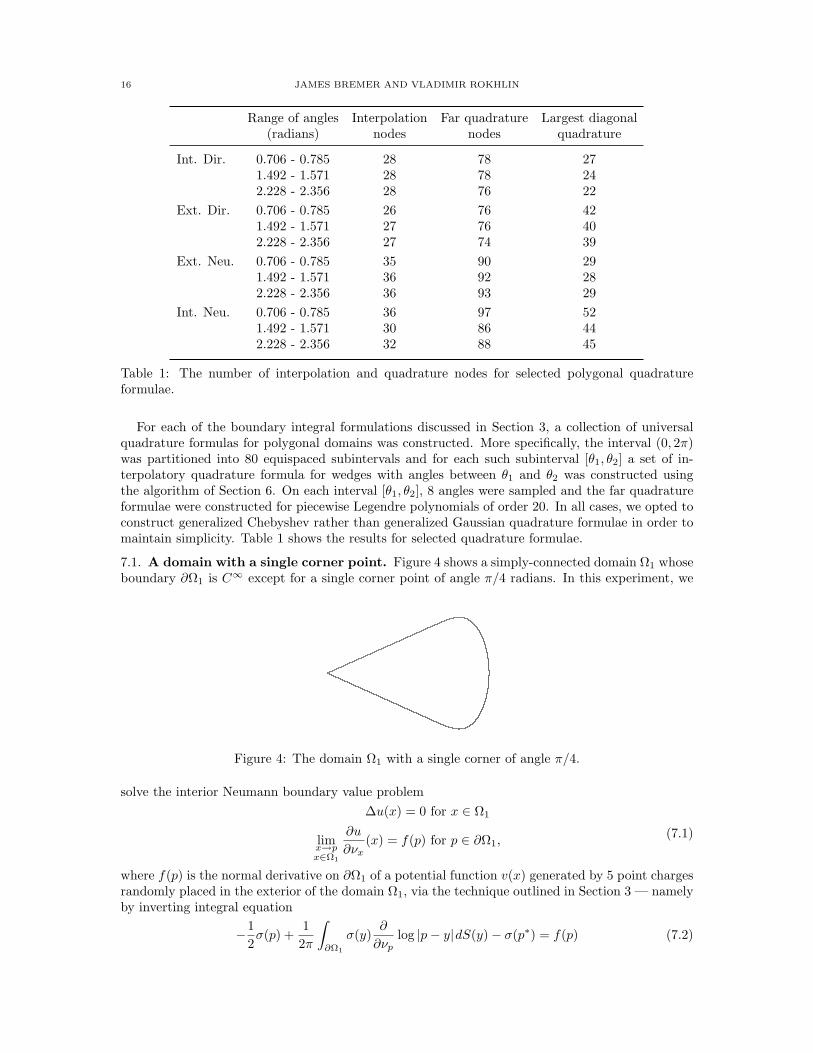
7.1. A domain with a single corner point. Figure 4 shows a simply-connected domain Ω1 whoseboundary ∂Ω1 is C∞ except for a single corner point of angle π/4 radians. In this experiment, we

Figure 4: The domain Ω1 with a single corner of angle π/4.

solve the interior Neumann boundary value problem∆u(x) = 0 for x ∈ Ω1

limx→px∈Ω1

∂u

∂νx(x) = f(p) for p ∈ ∂Ω1,

(7.1)

where f(p) is the normal derivative on ∂Ω1 of a potential function v(x) generated by 5 point chargesrandomly placed in the exterior of the domain Ω1, via the technique outlined in Section 3 — namelyby inverting integral equation

−12σ(p) +

12π

∫∂Ω1

σ(y)∂

∂νplog |p− y|dS(y)− σ(p∗) = f(p) (7.2)


in order to obtain a solution u of (7.1) in the form of a single layer potential

u(x) =1

2π

∫∂Ω1

log |x− y|σ(y)dS(y). (7.3)

Note that p∗ in (7.2) denotes an arbitrary point on the boundary curve; see Section 3.

N Tsolve Eabs Ecirc

Universal quadrature 216 0.006 3.12×10−14 8.82×10−15

Simply-graded mesh 520 0.081 4.07×10−06 2.30×10−07

800 0.275 1.52×10−10 8.58×10−11

1440 1.713 8.82×10−12 2.76×10−12

Table 2: Comparative performance of the universal quadrature formulas in solving an interiorNeumann problem on the domain Ω1.

Table 2 compares the results obtained by discretizing the integral equation (7.2) using a wedgequadrature formula with those obtained using the discretizations described in subsection 4.3. Inboth cases, the smooth portion of the curve were discretized using 180 piecewise Legendre interpo-lation nodes. The discrete systems were inverted using a simple direct solver for boundary integralequations which has asymptotic running time O(n2) in the number of discretization nodes n.• N is the total number of interpolation nodes used to discretize the integral equation (7.2);• Tsolve is the time required to invert the discrete linear system in seconds;• Eabs is the largest absolute error observed while measuring the difference between the computed

solution u(x) and the true potential function u(x) at a collection of 100 randomly placed pointsin the interior of the domain Ω1; and

• Ecirc is an approximation (obtained with a high order Gaussian quadrature) of the relative L2(Γ)error ‖u− v‖2/‖u‖2, where Γ is a circle of small radius located at the center of mass of ∂Ω1.

Remark 7.1. The boundary integral formulation (7.2) used here to solve the interior Neumannproblem is not necessary an optimal approach for domains with corners. There are many possibleways to modify a boundary integral formulation in order to reduce the complexity of such a problem;however, a notable advantage of the algorithm of this paper is that efficient quadratures can be ob-tained even using suboptimal boundary integral formulations. The precomputations can be performed,leisurely, in extended precision if need be and the resulting quadratures produce highly efficient andaccurate formulas, regardless of the underlying integral equation.

7.2. Two polygonal domains. In this subsection, we present results pertaining to the two polyg-onal domains shown in Figure 5. The domain Ω2 (pictured on the left) has 10 corner points ofvarious angles, while the domain Ω3 (pictured on the right) has 38 corner points.

For each of the Laplace boundary value problems discussed in Section 3, the correspondingintegral equation, which has the form

λσ(x) +∫

Γ

K(x, y)σ(y)dy = u(x),

was formed and discretized; the appropriate precomputed quadrature formula was used at eachcorner point and piecewise Legendre quadratures were used to discretize the smooth portions of thecurve. The right hand side u(x) was taken to be the restriction to the boundary of the domainof either a potential generated by a collection of 5 charges placed randomly either in the interioror exterior of the domain (depending on the boundary value problem under consideration), orthe normal derivative of such a potential function on the boundary of the domain. The discretesystems were inverted using a simple direct solver (with asymptotic complexity O(n2) in the number


(a) The domain Ω2. (b) The domain Ω3.

Figure 5: The polygonal domains under consideration in subsection 7.2.

of discretization nodes n). Figure 6 shows the dipole charge distribution on Ω3 obtained in thesolution of the interior Dirichlet problem. Table 3 presents the results for the polygonal domain Ω2

and Table 4 for the domain Ω3; the notation used is the same as that of the preceding section.

0

0.2

0.4

0.6

0.8

1

1.2

1.4

1.6

1.8

0 5 10 15 20 25 30 35 40

Figure 6: The continuous, but not smooth, dipole distribution on ∂Ω3 resulting from the solutionof the interior Dirichlet problem.

N TSolve Eabs Ecirc

Interior Dirichlet 847 0.364 4.48×10−15 1.17×10−14

Exterior Dirichlet 840 0.327 7.08×10−15 3.01×10−14

Exterior Neumann 926 0.437 5.50×10−15 2.74×10−14

Interior Neumann 900 0.391 3.71×10−15 2.98×10−14

Table 3: Computational results obtained for the polygonal domain Ω2.

N TSolve Eabs Ecirc





Table 4: Computational results obtained for the polygonal domain Ω3.


7.3. A polygonal domain with 250 vertices. In this example, we solve the exterior Neumannproblem

∆u(x) = 0 for x ∈ Ωc4

limx→px∈Ωc

4

∂u

∂νx(x) = f(p) for p ∈ ∂Ω4

(7.4)

on the polygonal domain Ω4 shown in Figure 7. The boundary of the domain Ω4 was obtained bysampling the smooth closed curve defined by the polar equation

r(θ) = 1 +12

cos(nθ) sin(mθ),

where n = 4 and m = 4, at 250 points. More specifically, the coordinates (xj , yj) of the vertices ofthe polygon ∂Ω4 are given by

xj =[1 +

12

cos(nθj) sin(mθj)]

cos(θj)

yj =[1 +

12

cos(nθj) sin(mθj)]

sin(θj)

where θj = 2πj/250, j = 1, 2, . . . , 250.

Figure 7: The polygonal domain Ω4, which was obtained by sampling a smooth curve at 250 points.

The boundary data f(p) was taken to be the normal derivative on ∂Ω4 of a potential functionv(x) generated by a collection of 10 point charges randomly placed in the interior of the domain Ω4.The boundary integral equation

12σ(p) +

12π

∫∂Ω4

∂

∂νxlog |p− y|σ(y)dS(y) = f(p) (7.5)

corresponding to the problem (7.4) was discretized as before; a total of 16341 discretization nodeswere required. The resulting discrete system was inverted in 61.0 seconds using a direct solver whichis asymptotically O(n2) in the number of discretization nodes n.

The true potential function v(x) was compared to the single layer potential

u(x) =1

2π

∫∂Ω4

log |x− y|σ(y)dS(y) (7.6)

arising from the charge distribution σ obtained by inverting (7.5) at 100 randomly chosen points inthe exterior of Ω4. The largest absolute error was found to be 2.23×10−14.


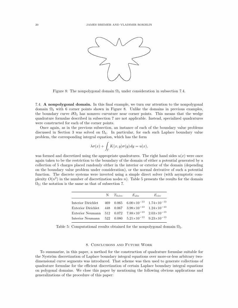
Figure 8: The nonpolygonal domain Ω5 under consideration in subsection 7.4.

7.4. A nonpolygonal domain. In this final example, we turn our attention to the nonpolygonaldomain Ω5 with 6 corner points shown in Figure 8. Unlike the domains in previous examples,the boundary curve ∂Ω5 has nonzero curvature near corner points. This means that the wedgequadrature formulas described in subsection 7 are not applicable. Instead, specialized quadratureswere constructed for each of the corner points.

Once again, as in the previous subsection, an instance of each of the boundary value problemsdiscussed in Section 3 was solved on Ω4. In particular, for each such Laplace boundary valueproblem, the corresponding integral equation, which has the form

λσ(x) +∫

Γ

K(x, y)σ(y)dy = u(x),

was formed and discretized using the appropriate quadratures. The right hand sides u(x) were onceagain taken to be the restriction to the boundary of the domain of either a potential generated by acollection of 5 charges placed randomly either in the interior or exterior of the domain (dependingon the boundary value problem under consideration), or the normal derivative of such a potentialfunction. The discrete systems were inverted using a simple direct solver (with asymptotic com-plexity O(n2) in the number of discretization nodes n). Table 5 presents the results for the domainΩ5; the notation is the same as that of subsection 7.

N TSolve Eabs Ecirc





Table 5: Computational results obtained for the nonpolygonal domain Ω5.

8. Conclusions and Future Work

To summarize, in this paper, a method for the construction of quadrature formulae suitable forthe Nystrom discretization of Laplace boundary integral equations over more-or-less arbitrary two-dimensional curve segments was introduced. That scheme was then used to generate collections ofquadrature formulae for the efficient discretization of certain Laplace boundary integral equationson polygonal domains. We close this paper by mentioning the following obvious applications andgeneralizations of the procedure of this paper:


• The generalization of the algorithm of Section 6 to boundary integral equations in three dimen-sions — that is, to equations of the form

λσ(x) +∫

Σ

K(x, y)σ(y)dS(y) = u(x) (8.1)

where Σ is a surface in R3 rather than a curve in R2 — is extremely straightforward. In particular,integral equations of this type can be discretized using generalizations of Gaussian polynomialsfor triangles. Given a small surface Σ0 contained in Σ discretized using a large number ofquadrature nodes, the integral equation (8.1) can be discretized and solved for right-hand-sidesconsisting of the terms of a three dimensional multipole expansion on Σ0 in order to form a localbasis for charge distributions on the surface Σ0. Efficient quadratures can then be constructedin essentially the same manner as described in Section 6.

• The approach detailed here for Laplace’s equation can be readily adapted to the case of boundaryvalue problems for the Helmholtz equation

∆u+ ω2u = 0,

assuming ω is not too large. Because the integral kernels for boundary integral equations arisingfrom the Helmholtz equation are weakly-singular instead of continuous, additional care mustbe taken in discretizing the integral equations. Moreover, the lack of scale invariance in theHelmholtz equation makes the construction of universal quadratures slightly more difficult. Oth-erwise, however, the algorithm for the Helmholtz case is analogous to that described here withthe role of the multipoles now played by the terms of the J-expansion∑

k

Jk(ωr) (αk sin(kθ) + βk cos(kθ)) ,

where Jk is the Bessel function of the first kind of order k.

• The algorithm presented here for the construction of universal quadrature rules for polygonaldomains can be extended to any setting for which the pathological behavior of the domains canbe classified efficiently. In particular, we expect to be able to extend the construction to muchmore general classes of domains with corner points.

• Similarly, in many engineering applications it is convenient to approximate boundary curves viaC2 splines. The discretization of a boundary integral equation

λσ(x) +∫

Γ

K(x, y)σ(y)dS(y) = u(x) (8.2)

over such a contour is, however, problematic — the lack of smoothness of spline functions severelylimits the order of convergence of discrete approximations of (8.2). But, by classifying thebehavior of C2 spline functions near singular points, it should be possible to construct a collectionof quadrature formulae for domains bounded by splines analogous to those constructed here forpolygonal domains.

• The quadrature construction algorithm can be used as a local solver for boundary integral equa-tions, allowing for a divide-and-conquer approach to the solution of boundary integral equationson extremely complicated domains. This can be, for instance, exploited to solve problems on do-mains which are sufficiently complicated that the resulting discrete systems might not otherwisefit in memory.

• Finally, we reiterate that the numerical experiments of Section 7 were conducted using a directsolver for boundary integral equations which is asymptotically O(n2) in the number of discretiza-tion nodes n. Coupling the approach of this paper with a faster technique for the inversion ofboundary integral equations (for instance, with the O(n) fast direct solver of [19]) will allow forthe solution of boundary integral equations on tremendously complicated domains.


9. Acknowledgments

The first author was supported by the Office of Naval Research under contract N00014-09-1-0318. The second author was supported in part by the ONR under contract N0014-07-1-0711, inpart by the AFOSR under contract FA9550-09 -1-0241, and in part by DARPA-AFOSR contractFA9550-07-1-0541.

References

[1] K. Atkinson, The Numerical Solution of Integral Equations of the Second Kind, Cambridge University Press,1997.

[2] K. E. Atkinson and I. Graham, Iterative variants of the Nystrom method for second kind boundary integral

operators, SIAM J. Sci. Stat. Comp., 13 (1990), pp. 694–722.[3] A. Bjorck, Numerical Methods for Least Squares Problems, SIAM, Philadephia, 1996.

[4] J. Bremer, Z. Gimbutas, and V. Rokhlin, A nonlinear optimization procedure for generalized Gaussian quadra-

tures, Yale University, Department of Computer Science Tech Report TR1406, 2008.[5] G. Chandler, Galkerin’s method for boundary integral equations on polygonal domains., J. Austral. Math. Soc.,

Series B, 26 (1984), pp. 1–13.[6] H. Cheng, V. Rokhlin, and N. Yarvin, Nonlinear optimization, quadrature, and interpolation, SIAM J. Optim,

9 (1999), pp. 901–923.

[7] R. Coifman and Y. Meyer, Wavelets: Calderon-Zygmund and multilinear Operators, Cambridge UniversityPress, 1997.

[8] E. Fabes, M. Jodeit, and N. Riviere, Potential theoretic techniques for boundary value problems on C1

domains, Acta. Math., 141 (1978), pp. 165–186.[9] G. Folland, Introduction to Partial Differential Equations, Princeton University Press, Princeton, N.J., 1976.

[10] P. Grisvard, Elliptic Problems in Nonsmooth Domains, Pitman, Boston, 1985.

[11] , Singularities in Boundary Value Problems, Springer-Verlag, 1992.[12] M. Gu and S. Eisenstat, Efficient algorithms for computing a strong rank-revealing QR factorization, SIAM

J. Sci. Comput., 17 (1996), pp. 848–869.

[13] J. Helsing and R. Ojala, Corner singularities for elliptic problems: integral equations, graded meshes, quad-rature, and compressed inverse preconditioning, Journal of Computational Physics, 227 (2008), pp. 8820–8840.

[14] O. Kellog, Foundations of Potential Theory, Dover, New York, 1953.[15] C. Kenig, Elliptic boundary value problems on Lipschitz domains, Beijing Lectures in Harmonic Analysis, Ann.

of Math. Stud., 112 (1986), pp. 131–183.

[16] R. Kress, A Nystrom method for boundry integral equations in domains with corners, Numerische Mathematik,58 (1991).

[17] , Integral Equations, Springer-Verlag, New York, 1999.

[18] J. Ma, V. Rokhlin, and S. Wandzura, Generalized Gaussian quadrature rules for systems of arbitrary func-tions, SIAM J. Numer. Anal., 33 (1996), pp. 971–996.

[19] P. Martinsson and V. Rokhlin, A fast direct solver for boundary integral equations in two dimensions, Journal

of Computational Physics, 205 (2006).[20] P.-G. Martinsson, V. Rokhlin, and M. Tygert, On interpolation and integration in finite-dimensional spaces

of bounded functions, Communications in Applied Mathematics and Computational Science, 1 (2006), pp. 133–142.

[21] S. Mikhlin, Integral Equations, Pergamon Press, New York, 1957.

[22] G. Verchota, Layer potentials and boundary value problems for Laplace’s equation in Lipschitz domains, Jour-nal of Functional Analysis, 59 (1984), pp. 572–611.

[23] N. Yarvin and V. Rokhlin, Generalized Gaussian quadratures and singular value decompositions of integral

operators, SIAM J. Sci. Comput., 20 (1998), pp. 699–718.

Documents

EFFICIENT DISCRETIZATION OF LAPLACE …bremer/papers/polygonal.pdfEFFICIENT DISCRETIZATION OF LAPLACE BOUNDARY INTEGRAL EQUATIONS ON POLYGONAL DOMAINS3 of domains for which universal