Embed Size (px)
Citation preview

Efficient Discrete-Time Simulations of Continuous-Time Quantum Query Algorithms
QIP 2009January 14, 2009
Santa Fe, NM
Rolando D. SommaJoint work with R. Cleve, D. Gottesman, M. Mosca, D. Yonge-Mallo

Query or Oracle Model of Computation
Given a black-box (BB)
€
x j ∈ {0,1} BB
€
j →
€
0 ≤ j ≤ N −1
For quantum algorithms, we consider a reversible version of BB:
€
j →
€
→ (−1)x j j
€
QX j = (−1)x j j
€
QX
Want to learn a property of the N-tuple
€
x0, x1,..., xN−1( )
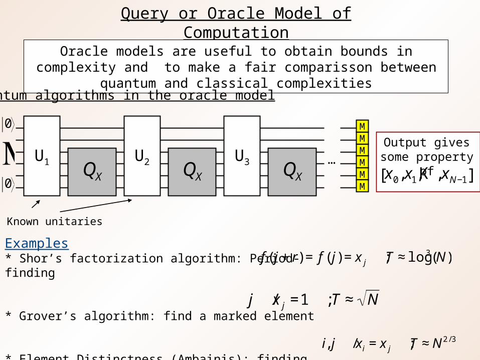
Query or Oracle Model of Computation
Oracle models are useful to obtain bounds in complexity and to make a fair comparisson between quantum and classical complexities
Quantum algorithms in the oracle model
U1 U2 U3 …
€
0
€
0
€
M
Known unitaries
Output gives some property of
€
x0,x1,K ,xN−1[ ]MMMMM
M
€
QX
€
QX
€
QX
Examples* Shor’s factorization algorithm: Period-finding
* Grover’s algorithm: find a marked element
* Element Distinctness (Ambainis): finding two equal items
€
f ( j + r) = f ( j) = x j ; T ≈ log3(N)
€
j / x j =1 ; T ≈ N
€
i, j / x i = x j ; T ≈ N 2 / 3

Continuous-Time Quantum Query Model of Computation
2- Time-dependent Driving Hamiltonian (known)
3- Evolution time (or total query cost) T>0
€
HD (t)
€
0
€
0
€
MOutput gives
some property of
€
x0, x1,K , xN−1[ ]
€
U = exp −i (HX + HD (t))dt0
T
∫ ⎡
⎣ ⎢
⎤
⎦ ⎥
MMMMM
M
€
j →
€
→ e-iH Xθ j
1- Query Hamiltonian
€
HX j = x j j
€
e−iH X π j = QX j = (−1)x j j
QXθ j = e−iHXθ j
€
QXθ
Query cost
fractional query
* E. Farhi and S. Gutmann, Phys. Rev. A 57, 2043 (1998)
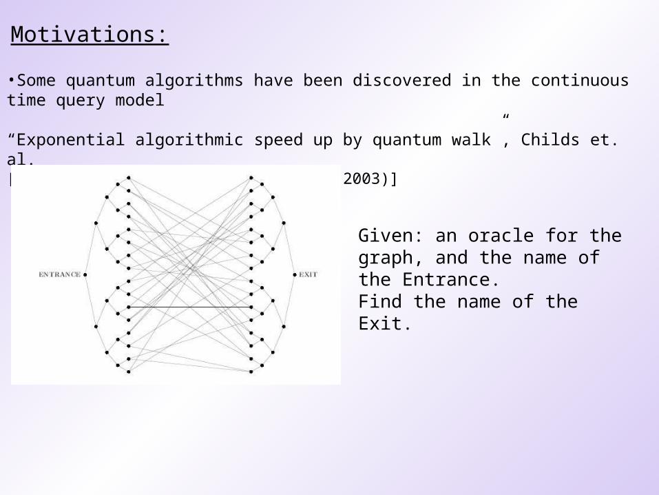
Motivations:
•Some quantum algorithms have been discovered in the continuous time query model
“Exponential algorithmic speed up by quantum walk”, Childs et. al.[Proc. 35th ACM Symp. On Th. Comp. (2003)]
Given: an oracle for the graph, and the name of the Entrance.Find the name of the Exit.

Motivations:
•Some quantum algorithms have been discovered in the continuous time query model
“A Quantum Algorithm for Hamiltonian NAND tree”, Farhi, Goldstone, Gutmann quant-ph/0702144
The query Hamiltonian is built from the adjacency matrix of a graph determined by the tree and the input state. It outputs the (binary) NAND in time
€
N
N

Motivations:
Is it possible to convert a quantum algorithm in the CT setting to a quantum algorithm in the more conventional query model?
We present a method to do it at a cost
€
T /ε( ) log(T /ε)
Yes:
It has been known(2) that this can be done with cost
€
eη HD T( )1+1/η
(2) D. Berry, G Ahokas, R. Cleve, and B.C. Sanders, Commun. Math. Phys. 270, 359 (2007)
Q(1): Is the CT query model more powerful than the conventional query model?
The actual implementation of a quantum algorithm in the CT setting may require knowledge on the query Hamiltonian which my not be an available resource.
(1) C. Mochon, Hamiltonian Oracles, quant-ph/0602032

MAIN RESULTS:
Theorem: Any continuous-time T-query algorithm can be
simulated by a discrete-time O(T log T )-query algorithm
Corollary: Any lower bounds on discrete query complexity carry over to continuous query complexity within a log factor
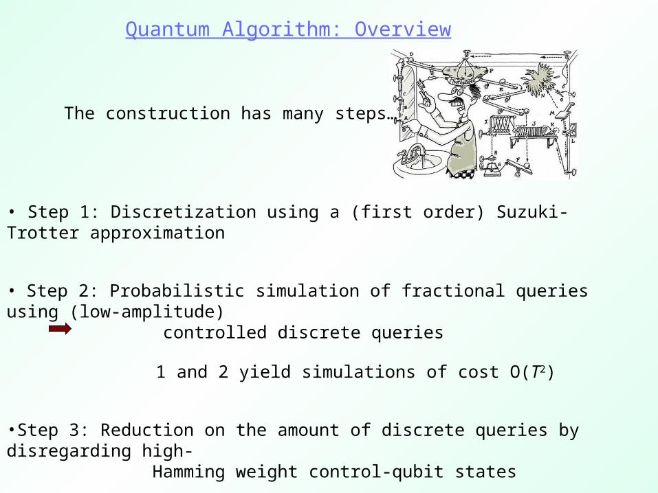
Quantum Algorithm: Overview
• Step 1: Discretization using a (first order) Suzuki-Trotter approximation
• Step 2: Probabilistic simulation of fractional queries using (low-amplitude) controlled discrete queries 1 and 2 yield simulations of cost O(T2)
•Step 3: Reduction on the amount of discrete queries by disregarding high- Hamming weight control-qubit states
• Step 4: Correction of errors due to step 2
The construction has many steps…
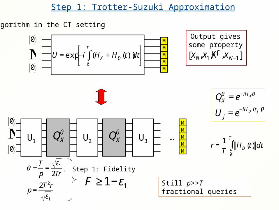
Step 1: Trotter-Suzuki Approximation
€
0
€
0
€
MOutput gives
some property of
€
x0, x1,K , xN−1[ ]
€
U = exp −i (HX + HD (t))dt0
T
∫ ⎡
⎣ ⎢
⎤
⎦ ⎥
Algorithm in the CT setting
MMMMM
U1 U2 U3…
€
0
€
0
€
M
€
QXθ
€
QXθ
€
QXθ = e−iH Xθ
U j = e−iH D ( t j )θ
€
θ =T
p=
ε1
2Tr;
p =2T 2r
ε1
€
F ≥1−ε1
Step 1: Fidelity
€
r =1
THD (t) dt
0
T
∫
Still p>>T fractional queries
MMMMM

Step 1: Trotter-Suzuki Approximation
U1 U2 U3…
€
0
€
0
€
M
€
QXθ
€
QXθ
€
QXθ = e−iH Xθ
U j = e−iH D ( t j )θ
€
θ =T
p=
ε1
2Tr;
p =2T 2r
ε1
€
F ≥1−ε1
Step 1: Fidelity
€
r =1
THD (t) dt
0
T
∫
Still p>>T fractional queries
MMMMM
€
QXθ
€
QX
€
QX€
+
€
e−iθ − −
It doesn’t work in general…

Step 2: Probabilistic Simulation of Fractional Queries
€
QXθ = e−iH Xθ = e−iθ / 2 cos(θ /2)1+ isin(θ /2)QX[ ]
€
QX = e−iH X π
€
0 → QXθ Pr. success : ps ≥1−θ
1 → QX−π / 2 Pr. failure : p f ≤ θ
€
QXθ
€
QX
R1 R2
€
0 M
€
cos(θ /2) 0 + i sin(θ /2)
€
R2 :0 a cos(θ /2) 0 + sin(θ /2) 1
1 a sin(θ /2) 0 − cos(θ /2) 1
⎧ ⎨ ⎪
⎩ ⎪
Why do we want this conversion?
€
p =2T 2r
ε1
>> T;
θ =T
p=
ε1
2Tr<<1
The actual query cost is much lower than p.In step 3, we take advantage of this situation.
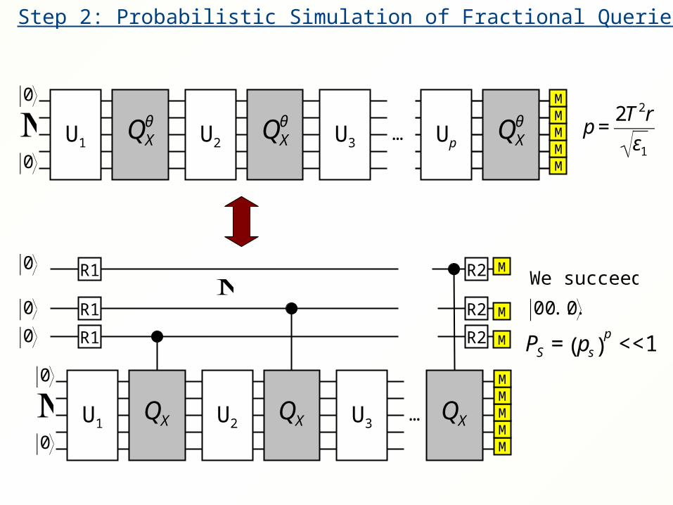
Step 2: Probabilistic Simulation of Fractional Queries
U1 U2 U3…
€
0
€
0
€
M
€
QXθ
€
QXθ
MMMMM
€
0
U1 U2 U3…
€
0
€
0
€
MMMMMM
R1
R1
R1
M
M
M
€
QX
€
QX
R2
R2
R2
€
We succeed if
00...0
€
PS = ps( )p
<<1
€
M
€
QX
€
0
€
0
€
p =2T 2r
ε1Up
€
QXθ

Step 3: Reducing the amount of queries
m queries
€
P'S = ps( )m
≥ (1−θ)m = 3/4 For a segment of size m,it is likely to succeed
€
m =1
4θ=
Tr
2 ε1
<< p =2T 2r
ε1
There are 4T segments of that sizein the total circuit
We break the circuit in segments of size m :
€
0
U1 U2 U3…
€
0
€
0
€
MMMMMM
R1
R1
R1
M
M
M
€
QX
€
QX
R2
€
We succeed if
00...0
€
PS = ps( )p
<<1
€
M
€
QX
€
0
€
0 R2
R2€
0 R1 MR2…
€
M
€
M

Step 3: Reducing the amount of queries
U1 U2 U3…
€
0
€
0
€
M
R1
R1
R1
M
M
M
€
QX
€
QX
R2
R2
R2€
Success if 0⊗m
€
P'S ≥ 3/4
m queries
m
€
∝ cos(θ /2) 0 + i sin(θ /2) 1( )⊗m
Density of states
€
M
Hamming weight
Poisson distribution: Exponential decay
€
Expected value of HW : A ≈ mθ ≈1/4
Um
€
QX
€
m =1
4θ

Step 3: Reducing the amount of queries
U1 U2 U3…
€
0
€
0
€
M
R1
R1
R1
€
QX
€
QX
€
M
m queries
m
€
QX
Density of states
Average: A<1/2
Hamming weight cutoff
€
k ∈ O log(T /ε2)[ ]
€
Fidelity :
F ≥1−ε2
At most k<<m full queries are needed !

Step 3: Reducing the amount of queries
U1 U2 U3 …
€
0
€
0
€
M
R1
R1
R1
€
QX
€
QX
€
Mm
€
QXm full queries
V2 V3 …
€
0
€
0
€
M
R1
R1
R1
€
QX
€
QX
€
Mm
€
QX Vk
full queries
U1
€
k ∈ O(log(T /ε2)) << m

Step 3: Reducing the amount of queries
Vj
m
Asks the value of the Hamming weight
Implements the desired sequence of U’s
V2
m
Example:
€
If in 00...0
€
Implement U2 , U3 , ..., Um
U2 U3 Um
€
M
€
M
€
M
…

Step 3: Reducing the amount of queries
€
So far, if we replace the circuit as explained in step 3,
the total amount of full queries is ( p /m)log(T /ε2)∝ T /ε1( )log(T /ε2)
€
However, the probability of success is still
PS = pS( )p
≈ (1−θ)p <<1
We build Step 4 to error correct and increase the probability of success towards 1

Step 4: Error correction
U1 U2 U3…
€
0
€
0
€
M
R1
R1
R1
€
QX
€
QX
€
M
m queries
m
€
QX€
We succeed if
0⊗m
€
P'S = ps( )m
≥1/4M
M
M
€
A failure (i.e., 1 ) is equivalent to perform the
operation QXπ / 2 instead of the desired operation QX
θ
X
€
QXθ Um ...QX
−π / 2U j ...QXθ U2QX
θ U1
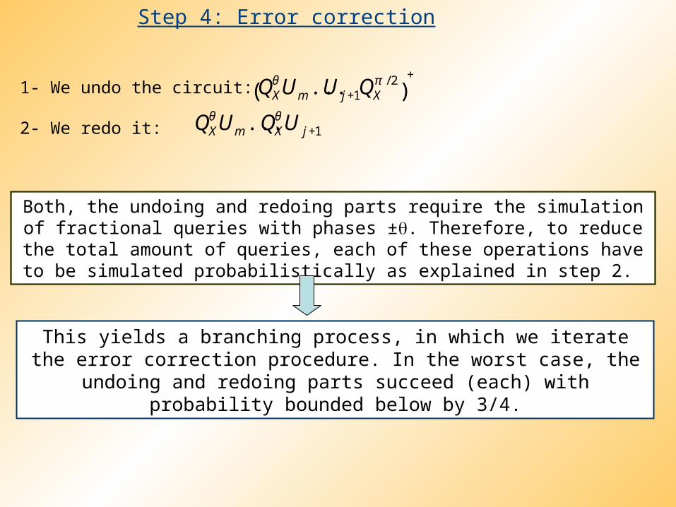
1- We undo the circuit:
2- We redo it:
€
QXθ Um ...U j +1QX
−π / 2( )
+
€
QXθ Um ...QX
θ U j +1
Step 4: Error correction
1- We undo the circuit:
2- We redo it:
€
QXθ Um ...U j +1QX
π / 2( )
+
€
QXθ Um ...QX
θ U j +1
Both, the undoing and redoing parts require the simulation of fractional queries with phases ± . Therefore, to reduce the total amount of queries, each of these
operations have to be simulated probabilistically as explained in step 2.
This yields a branching process, in which we iterate the error correction procedure. In the worst case, the undoing and redoing parts succeed
(each) with probability bounded below by 3/4.
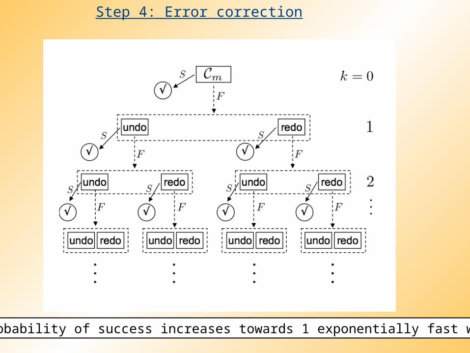
Step 4: Error correction
The probability of success increases towards 1 exponentially fast with k
Step 4: Error correction
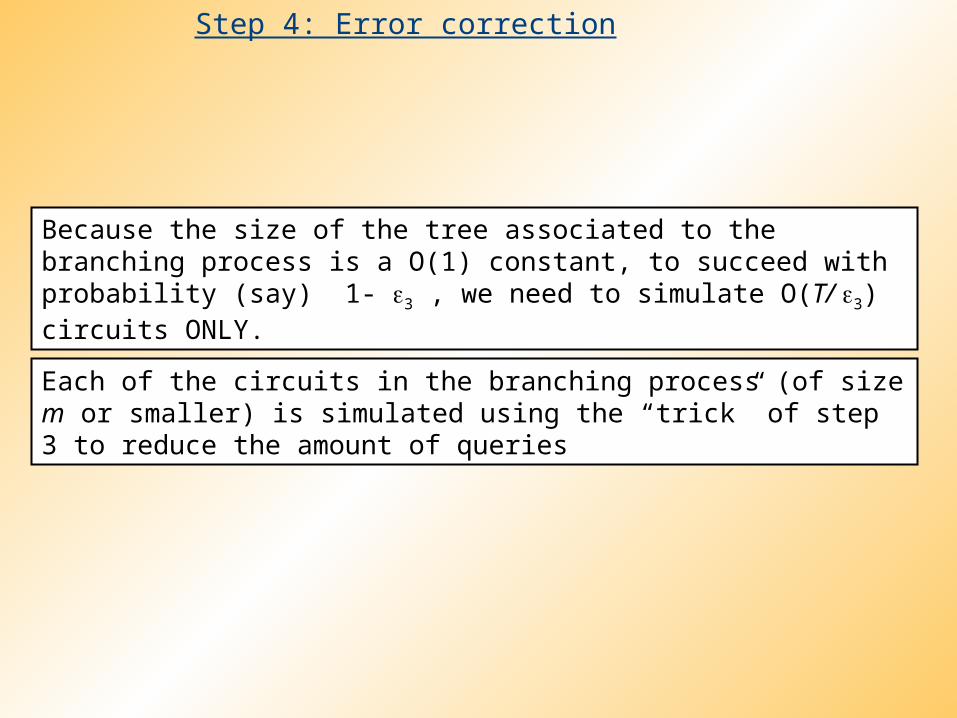
Each of the circuits in the branching process (of size m or smaller) is simulated using the “trick” of step 3 to reduce the amount of queries
Because the size of the tree associated to the branching process is a O(1) constant, to succeed with probability (say) 1- 3 , we need to simulate O(T/ 3) circuits ONLY.

Complexity of the simulation
For fidelity 1-, our simulation requires full queries
€
O[log(T /ε)(T /ε)]
€
O[log(T /ε)T log(1/ε)]For classical input/output, the overall complexity is
€
We choose ε1 , ε2 , ε3 , which correspond to the errors from
the Trotter approximation, Hamming weight cutoff, and the prob.
of failure in the simulation of the branching process, of order ε

Step 5: Conclusions!
€
Described an efficient discrete query simulation of continuous- time query algorithms
with complexity O(T log(T /ε)log(1/ε)), for fidelity 1- ε
€
The amount of known unitaries required is of order O(rT 2 log(T /ε)),
but this is not essential (depends on behavior of driving Hamiltonian)
Improvements?