Efficient Computational Techniques in Bioimpedance

1. Introduction

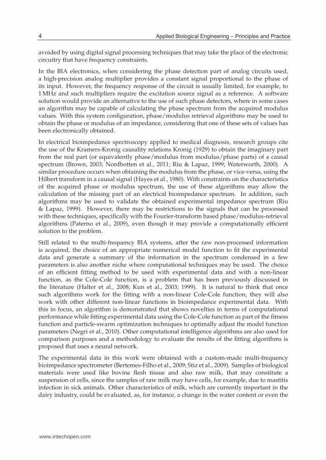
Electrical Bioimpedance Analysis (BIA) is an important tool in the characterization of organicand biological material. For instance, its use may be mainly observed in the characterizationof biological tissues in medical diagnosis (Brown, 2003), in the evaluation of organic andbiological material suspensions in biophysics (Cole, 1968; Grimnes & Martinsen, 2008),in the determination of fat-water content in the body (Kyle et al., 2004) and in in vivoidentification of cancerous tissues (Aberg et al., 2004), to name a few important works. It isalso natural to have different computational approaches to bioimpedance systems since morecomplex computational techniques are required to reconstruct images in electrical impedancetomography (Holder, 2004), and this would open a myriad of other computational andmathematical questions based on inverse reconstruction problems.

In many practical cases, the obtained bioimpedance spectrum requires that the producedsignal be computationally processed to guarantee the quality of the information containedin it, or to extract the information in a more convenient way. Such algorithms would allow theremoval of redundant data or even the suppression of invalid data caused by artifacts in thedata acquisition process. Many of the discussed computational methods are also applied inother areas that use electrical impedance spectroscopy, as in chemistry, materials sciences andbiomedical engineering (Barsoukov & Macdonald, 2005).

BIA systems allow the measurement of an unknown impedance across a predeterminedfrequency interval. In a typical BIA system, the organic or biological material suspension ortissue sample to be characterized is excited by a constant amplitude sine voltage or current andthe impedance is calculated at each frequency after the other parameter, current or voltage,is measured. This technique is called sine-correlation response analysis and can provide ahigh degree of accuracy in the determination of impedances. By using the sine-correlationtechnique, the spectrum is determined either by obtaining the impedance real and imaginaryparts, or by directly obtaining its modulus and phase. For this purpose, analog precisionamplifiers and phase detectors provide signals proportional to modulus and phase at eachfrequency, and the interrogated frequency range is usually between 100 Hz up to 10 MHz. Insuch BIA systems the current signal used in the sample excitation is band-limited, becausethe output impedance of the current source and the open-loop gain of its amplifiers arelow, especially at high frequencies (Bertemes-Filho, 2002). Some of these limitations may be

Efficient Computational Techniques in Bioimpedance Spectroscopy

Aleksander Paterno, Lucas Hermann Negri and Pedro Bertemes-Filho Department of Electrical Engineering, Center of Technological Sciences

Santa Catarina State University, Joinville, Brazil

1

www.intechopen.com

2 Will-be-set-by-IN-TECH

avoided by using digital signal processing techniques that may take the place of the electroniccircuitry that have frequency constraints.

In the BIA electronics, when considering the phase detection part of analog circuits used,a high-precision analog multiplier provides a constant signal proportional to the phase ofits input. However, the frequency response of the circuit is usually limited, for example, to1 MHz and such multipliers require the excitation source signal as a reference. A softwaresolution would provide an alternative to the use of such phase detectors, where in some casesan algorithm may be capable of calculating the phase spectrum from the acquired modulusvalues. With this system configuration, phase/modulus retrieval algorithms may be used toobtain the phase or modulus of an impedance, considering that one of these sets of values hasbeen electronically obtained.

In electrical bioimpedance spectroscopy applied to medical diagnosis, research groups citethe use of the Kramers-Kronig causality relations Kronig (1929) to obtain the imaginary partfrom the real part (or equivalently phase/modulus from modulus/phase parts) of a causalspectrum (Brown, 2003; Nordbotten et al., 2011; Riu & Lapaz, 1999; Waterworth, 2000). Asimilar procedure occurs when obtaining the modulus from the phase, or vice-versa, using theHilbert transform in a causal signal (Hayes et al., 1980). With constraints on the characteristicsof the acquired phase or modulus spectrum, the use of these algorithms may allow thecalculation of the missing part of an electrical bioimpedance spectrum. In addition, suchalgorithms may be used to validate the obtained experimental impedance spectrum (Riu& Lapaz, 1999). However, there may be restrictions to the signals that can be processedwith these techniques, specifically with the Fourier-transform based phase/modulus-retrievalalgorithms (Paterno et al., 2009), even though it may provide a computationally efficientsolution to the problem.

Still related to the multi-frequency BIA systems, after the raw non-processed informationis acquired, the choice of an appropriate numerical model function to fit the experimentaldata and generate a summary of the information in the spectrum condensed in a fewparameters is also another niche where computational techniques may be used. The choiceof an efficient fitting method to be used with experimental data and with a non-linearfunction, as the Cole-Cole function, is a problem that has been previously discussed inthe literature (Halter et al., 2008; Kun et al., 2003; 1999). It is natural to think that oncesuch algorithms work for the fitting with a non-linear Cole-Cole function, they will alsowork with other different non-linear functions in bioimpedance experimental data. Withthis in focus, an algorithm is demonstrated that shows novelties in terms of computationalperformance while fitting experimental data using the Cole-Cole function as part of the fitnessfunction and particle-swarm optimization techniques to optimally adjust the model functionparameters (Negri et al., 2010). Other computational intelligence algorithms are also used forcomparison purposes and a methodology to evaluate the results of the fitting algorithms isproposed that uses a neural network.

The experimental data in this work were obtained with a custom-made multi-frequencybioimpedance spectrometer (Bertemes-Filho et al., 2009; Stiz et al., 2009). Samples of biologicalmaterials were used like bovine flesh tissue and also raw milk, that may constitute asuspension of cells, since the samples of raw milk may have cells, for example, due to mastitisinfection in sick animals. Other characteristics of milk, which are currently important in thedairy industry, could be evaluated, as, for instance, a change in the water content or even the

4 Applied Biological Engineering – Principles and Practice

www.intechopen.com

Efficient Computational Techniques in Bioimpedance Spectroscopy 3

presence of an illegal adulterant, like hydrogen peroxide (Belloque et al., 2008). The problemwas then to characterize the raw milk with such adulterants using the bioimpedance spectrumeither fitted to a Cole-Cole function or not (Bertemes-Filho, Valicheski, Pereira & Paterno,2010). The neural network algorithm may be in this particular case a useful technique toclassify the milk with hydrogen peroxide (Bertemes-Filho, Negri & Paterno, 2010).

As a summary, the authors provided a compilation of problems into which computationalintelligence and digital signal processing techniques may be used, as well as the illustrationof new methodologies to evaluate the processed data and consequently the proposedcomputational techniques in bioimpedance spectroscopy.

2. Materials and methods

2.1 The BIA system to interrogate bioimpedances

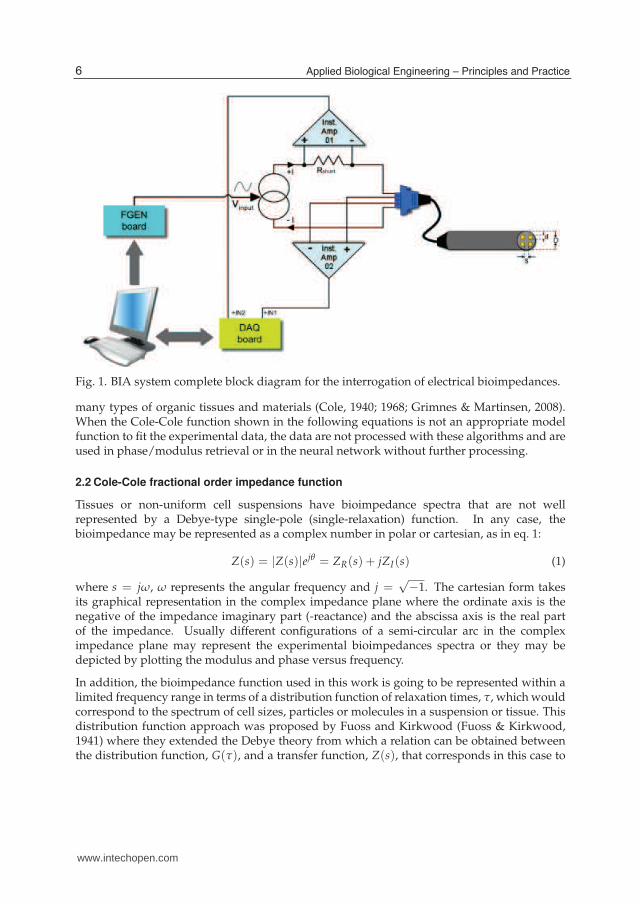
The used BIA system is based on a bioimpedance spectrometer consisting of a current sourcethat injects a variable frequency signal into a load by means of two electrodes. It thenmeasures the resulting potential in the biological material sample with two other electrodesand calculates the transfer impedance of the sample. The complete block diagram of thespectrometer system is shown in fig. 1. A waveform generator (FGEN) board supplies asinusoidal signal with amplitude of 1 Vpp (peak-to-peak) in the frequency range of 100 Hzto 1 MHz. The input voltage (Vinput) is converted to a current (+I and −I) by a modifiedbipolar Howland current source (also known as voltage controlled current source) (Stiz et al.,2009), which injects an output current of 1 mApp by two electrodes to the biological materialunder study. The resulting voltage is measured with a differential circuit between the othertwo electrodes by using a wide bandwidth instrumentation amplifier (Inst. Amp. 02). Theamplitude of the injecting current is measured by another instrumentation amplifier (Inst.Amp. 01) while using a precision shunt resistor (Rshunt) of 100 Ω. A custom made tetrapolarimpedance probe was used to measure the bioimpedance and is composed of 4 triaxialcables. The outer and inner shields of the cables are connected together to the ground ofthe instrumentation. The tip of the probe has a diameter of 8 mm (D), and the electrodematerial is a wire of 9 carat gold with a diameter of 1 mm (d). The wires are disposed ina circular formation about the longitudinal axis. Finally, a data acquisition (DAQ) boardmeasures both voltage load and output current by sampling the signals at a maximumsampling frequency of 1.25 MSamples/s for each of the possible 33 frequencies in the range.Data are stored in the computer for the processing of the bioimpedance spectra. Althoughthe modulus and phase of the load are electronically obtained, one of the parameters can beused to experimentally validate the phase/modulus retrieval technique while comparing thecalculated and measured values.

For completeness purposes, if one decides to use the bioimpedance spectrum points atfrequencies which were not used in the excitation or were not acquired, the value at thisfrequency can be determined by means of interpolation, since the evaluated spectra areusually well-behaved.

The nature of the experimental bioimpedance spectra is important for the use of thealgorithms described in this work. It is assumed here that the experimental samplebioimpedance spectrum may have its points represented by a Cole-Cole function in theinterrogated frequency range. This is a plausible supposition, since it is a function thatrepresents well many types of bioimpedance spectra associated with cell suspensions and

5Efficient Computational Techniques in Bioimpedance Spectroscopy

www.intechopen.com


Fig. 1. BIA system complete block diagram for the interrogation of electrical bioimpedances.

many types of organic tissues and materials (Cole, 1940; 1968; Grimnes & Martinsen, 2008).When the Cole-Cole function shown in the following equations is not an appropriate modelfunction to fit the experimental data, the data are not processed with these algorithms and areused in phase/modulus retrieval or in the neural network without further processing.

2.2 Cole-Cole fractional order impedance function

Tissues or non-uniform cell suspensions have bioimpedance spectra that are not wellrepresented by a Debye-type single-pole (single-relaxation) function. In any case, thebioimpedance may be represented as a complex number in polar or cartesian, as in eq. 1:

Z(s) = |Z(s)|ejθ = ZR(s) + jZI(s) (1)

where s = jω, ω represents the angular frequency and j =√−1. The cartesian form takes

its graphical representation in the complex impedance plane where the ordinate axis is thenegative of the impedance imaginary part (-reactance) and the abscissa axis is the real partof the impedance. Usually different configurations of a semi-circular arc in the compleximpedance plane may represent the experimental bioimpedances spectra or they may bedepicted by plotting the modulus and phase versus frequency.

In addition, the bioimpedance function used in this work is going to be represented within alimited frequency range in terms of a distribution function of relaxation times, τ, which wouldcorrespond to the spectrum of cell sizes, particles or molecules in a suspension or tissue. Thisdistribution function approach was proposed by Fuoss and Kirkwood (Fuoss & Kirkwood,1941) where they extended the Debye theory from which a relation can be obtained betweenthe distribution function, G(τ), and a transfer function, Z(s), that corresponds in this case to


www.intechopen.com


a bioimpedance. This relation is given by:

Z(s) =∫ ∞

0

G(τ)

1 + sτdτ (2)

By using eq.2, the relation between Z(s) and G(τ) is stressed:

Z f rac(s) =R0 − R∞

1 + (sτ0)α= (R0 − R∞)

∫ ∞

0

G(τ)

1 + sτdτ (3)

In eq. 3, the frequency dependent part of the impedance in the Cole-Cole type model function,Z f rac(s), is represented, where R0 is the impedance resistance at very low frequencies, R∞

is the resistance at very high frequencies, and the function containing the fractional orderterm, (sτ0)

α can be represented by an integral of the distribution function G(τ) (Cole & Cole,1941), and α is a constant in the interval [0, 1] and τ0 is the generalized relaxation time. G(τ)is a distribution function for the fractional order Cole-Cole model function and is explicitlyrepresented by Cole & Cole (1941):

G(τ) =1

2π

⎡

⎣

sin [(1 − α)π]

cosh[

α log( ττ0)]

− cos [(1 − α)π]

⎤

⎦ (4)

The complete model developed by Cole and Cole consists of an equation, an equivalent circuitand a complex impedance circular arc locus, and in terms of impedances, after integratingeq. 3, one obtains the Cole-Cole function to represent the evaluated impedance spectrum:

ZCole(ω) = R∞ +R0 − R∞

1 + (jωτ0)α(5)

In eq. 5, the variable ZCole(ω) is a complex impedance and is a function of the angularfrequency ω. The Cole-Cole function was obtained by the Cole and Cole brothers whenthey also introduced the distribution function of eq. (4). It is worth noticing that the functioncontaining the fractional order term, (sτ0)

1−α instead of the (sτ0)α, was originally used in a

model for dielectrics (Cole & Cole, 1941).

For the use of the phase/modulus retrieval algorithm in ZCole(s) the independent termcorresponding to the resistance, R∞, causes the frequency dependent function to satisfyneither the phase- nor the modulus-retrieval algorithm conditions (Hayes et al., 1980; Paternoet al., 2009). In other words, the experimental points to be used with the phase/modulusretrieval algorithm must be previously tested with known bioimpedance spectrum data toverify if the process is applicable. Consequently, the algorithm has limitations of use if theresistance at very high frequencies is not zero, or if the condition of minimum phase in thespectrum is not satisfied. In addition to that, for the reconstruction of phase and modulusof ZCole(s), the experimental data must correspond to a Cole-Cole spectrum that may befitted to a specific set of values of α (Paterno et al., 2009), otherwise the algorithm maynot converge to the correct values. Fortunately, these values of α with which the algorithmproperly works correspond to a broad class of tissues, cell suspensions and organic materialsto be evaluated in practical cases. In the limit, when α ≈ 0, Z f rac(s) becomes a pure resistancehaving minimum-phase. For values of α in the interval (0, 1), the modulus retrieval algorithmmay be capable of producing a limited error, as demonstrated elsewhere (Paterno et al.,


www.intechopen.com


2009). For the use of instrumentation to characterize the spectrum of organic material, thisconditions are usually met, as in the illustration case of bioimpedances obtained from mango,banana, potato and guava, shown in the results in section 3. These are illustrative examplesof organic material to have its impedance phase measured and used as input to the algorithmthat determines the bioimpedance modulus. In this case, both parameters were measured tovalidate the results (Paterno & Hoffmann, 2008).

2.3 Phase/modulus retrieval algorithm description

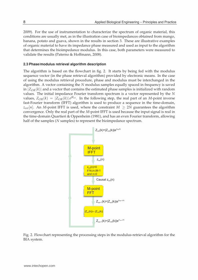
The algorithm is based on the flowchart in fig. 2. It starts by being fed with the modulussequence vector (in the phase retrieval algorithm) provided by electronic means. In the caseof using the modulus retrieval procedure, phase and modulus must be interchanged in thealgorithm. A vector containing the N modulus samples equally spaced in frequency is savedin |ZOR(k)| and a vector that contains the estimated phase samples is initialized with randomvalues. The initial impedance Fourier transform spectrum is a vector represented by the Nvalues, ZOR(k) = |ZOR(k)| ejθest . In the following step, the real part of an M-point inversefast-Fourier transform (IFFT) algorithm is used to produce a sequence in the time-domain,zest[n]. An M-point IFFT is used, where the constraint M ≥ 2N guarantees the algorithmconvergence. Only the real part of the M-point IFFT is used because the input signal is real inthe time-domain Quartieri & Oppenheim (1981), and has an even Fourier transform, allowinghalf of the samples (N samples) to represent the bioimpedance spectrum.

z (n)est

M-pointIFFT

Z (k)=|Z (k)|eOR OR

j (k)�est

Z (k)=|Z (k)|eest+1 est

j (k)�est+1

Z (k)=|Z (k)|eest+1 OR

j�est+1(k)

z

0

est(n)=0

if N n M-1

and n

� �

�

M-pointFFT

|Z (k)| |Z (k)|est OR�

Causal z (n)est

Fig. 2. Flowchart representing the processing steps in the modulus-retrieval algorithm for theBIA system.


www.intechopen.com


Causality is imposed in the fourth block while a finite length constraint on the time-domainsequence sets zest(n) to zero for n > N − 1. The M-point FFT of the data set containing z(n)produces the estimates of the bioimpedance spectrum. This flowchart indicates the processthat is repeated until the root-mean squared value of the difference between two consecutiveestimated vectors is less than a stopping parameter, ǫ. It was set equal to ǫ = 10−6, whichis a much lower value than the necessary modulus or phase resolution in BIA systems. Thelength of the input vector sequences is a power of 2, since the iterative solution uses uniformlyspaced samples Quartieri & Oppenheim (1981) and the Fast-Fourier Transform (FFT) radix-2algorithm (Proakis & Manolakis, 2006).

2.4 Computational intelligence algorithms in electrical bioimpedance spectroscopy

In this section computational intelligence algorithms will be briefly described such as to beused in an application to fit experimental data obtained with BIA systems using particleswarm optimization techniques; additionally, artificial neural networks (ANN) are describedto provide a methodology to evaluate the fitting algorithms. The performance testing isimplemented by associating the training phase of the ANN to previously known informationcontained in the bioimpedance spectrum. For example, in the evaluated sample. The presenceof different adulterants in raw milk, specifically water and hydrogen peroxide, and thecharacterization of the type of bovine flesh tissue are samples that were interrogated withthe BIA system. The ANN is used to evaluate how much information the fitting process mayextract from the experimental data such as to condense it into the parameters of the usedfunction model, namely, the Cole-Cole function that contains four parameters (R0, R∞, τ andα) as in eq.5 with the information of the electrical bioimpedance spectrum.

2.4.1 The Particle-Swarm Optimization (PSO) experiment

The particle swarm optimization algorithm was used to extract the Cole-Cole functionparameters, R0, R∞, τ0 and α from experimental data. For this experiment, the previouslydescribed bioimpedance spectrometer injected a sinusoidal current via the two electrodesof a tetrapolar probe into bovine liver, heart, topside, and back muscle samples. A cowwas killed in a slaughterhouse, where the samples were extracted and immediately headedto the laboratory where the bioimpedance measurements were performed. The measuredbioimpedance spectrum points contained 32 modulus and phase values at frequencies inthe range from 500 Hz up to 1 MHz. A set of 20 pairs of reactance and resistance pointscorresponding to the lowest frequencies (from 500 Hz up to 60 kHz) was processed with aPSO algorithm.

2.4.1.1 The PSO algorithm

PSO is inspired by bird flocking, where one may consider a group of birds that movesthrough the space searching for food, and that uses the birds nearer to the goal (food) asreferences (Xiaohui et al., 2004). PSO algorithms to fit a known function to experimental datais a technique similar to the one using genetic algorithms (GA). PSO has however a fasterconvergence for unconstrained problems with continuous variables such as the addressedfitting problem of the Cole-Cole function and has a simple arithmetic complexity (Hassanet al., 2005). Briefly, the PSO algorithm can be separated in the following steps:

1. Population initialization;


www.intechopen.com


2. Evaluation of the particles in the population by a heuristic function, where in this case theparticles are formed by a vector with the Cole-Cole function parameters;

3. Selection of the fittest particles (set of parameters) to lead the population towards the bestset and

4. Update of the position and velocity of each particle by repeating the steps from 2 to 4 untila stopping condition is satisfied (Xiaohui et al., 2004).

Each parameter of the optimized function, in this case the fitting of the Cole-Cole function ineq. 5 to an experimental bioimpedance spectrum, can be represented as one dimension in thesearch space. The velocity update rule for the i-th particle is given by:

vid = w × vid + c1 × rand()× (pid − xid) + c2 × rand()× (pnd − xid) (6)

where vid is the velocity of the i-th particle in the dimension d; w is the inertia weight, in the[0, 1) range; c1 and c2 are the learning rates, usually in the [1, 3] range; rand() is a randomnumber in the [0, 1] interval, pid is the best position of the i-th particle for the d-th dimensionand pnd is the best neighborhood position for the d-th dimension. The particle position isupdated by summing the present position to the velocity.

Each particle is made by a vector with the parameters [R0, R∞, τ0, α] of the Cole-Cole function,that are randomly initialized with arbitrary values in an interval corresponding to the physicallimits of the system. A parameter restart step for the global search, inspired by the geneticalgorithm mutation operator, was added to the code to prevent the premature convergence ofthe algorithm.

Like a genetic algorithm, the PSO enhances the solution based on a heuristic function, namedfitness function, that measures the difference between the experimental spectrum and thefitted one. The fitness function is shown in eq. 7

f itness(p) = − 1N

N

∑i=1

abs(Zi − Ai)2 (7)

It is defined by the modulus of the difference between the original complex bioimpedanceexperimental points, Zi, and the fitted spectrum, Ai. As a consequence, resistance andreactance are taken into account in the function, and therefore, in the fitting.

2.4.2 Artificial neural networks and the fitted functions of the bioimpedance spectrum

Artificial neural networks (ANN) were implemented such as to evaluate the behavior of thefitting algorithms to experimental data. This was developed to determine, comparatively, howmuch information the extracted parameters from the fitted Cole-Cole function may containthat represents correctly the experimental bioimpedances.

2.4.2.1 ANN as used in BIA

One of the important features of a neural network resides in its capability to learn therelationships in a given data mapping, such as the mapping from the bioimpedance spectrato the type of the analyzed sample. This feature allows the network to be trained to performestimations and classify new samples according to the learned pattern.


www.intechopen.com


An ANN is composed of interconnected artificial neurons, each neuron being a simplecomputer unit (Haykin, 1999). Although a single neuron can perform only a simple operation,the network computational power is significant (Cybenko, 1989; Gorban, 1998) and can tackleany computable problem (Siegelmann & Sontag, 1991), under certain circumstances.

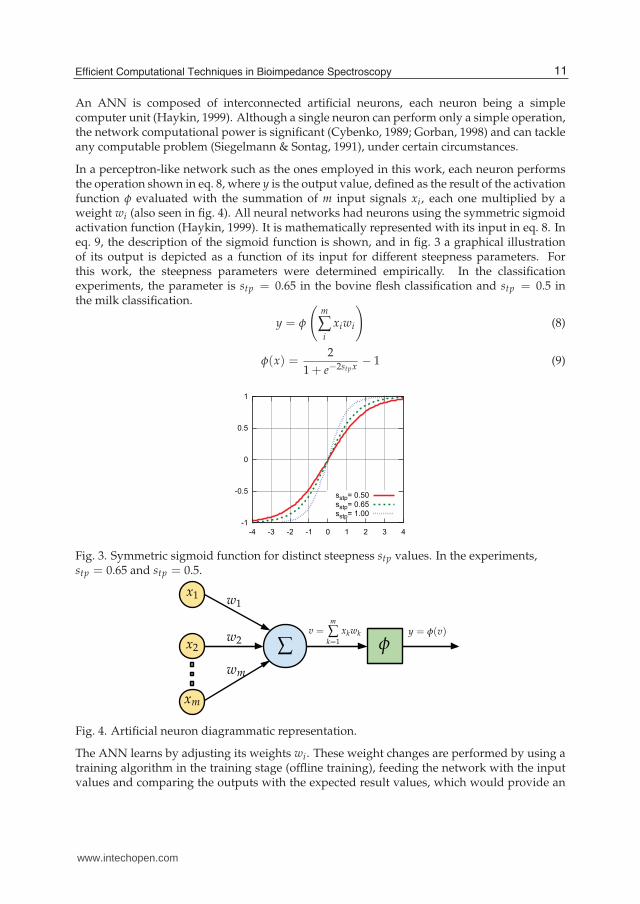
In a perceptron-like network such as the ones employed in this work, each neuron performsthe operation shown in eq. 8, where y is the output value, defined as the result of the activationfunction φ evaluated with the summation of m input signals xi, each one multiplied by aweight wi (also seen in fig. 4). All neural networks had neurons using the symmetric sigmoidactivation function (Haykin, 1999). It is mathematically represented with its input in eq. 8. Ineq. 9, the description of the sigmoid function is shown, and in fig. 3 a graphical illustrationof its output is depicted as a function of its input for different steepness parameters. Forthis work, the steepness parameters were determined empirically. In the classificationexperiments, the parameter is stp = 0.65 in the bovine flesh classification and stp = 0.5 inthe milk classification.

y = φ

(

m

∑i

xiwi

)

(8)

φ(x) =2

1 + e−2stp x− 1 (9)

!

"#$

"

"#$

!

% & ' ! " ! ' & %

(()*+,"#$"(()*+,"#-$(()*+,!#""

Fig. 3. Symmetric sigmoid function for distinct steepness stp values. In the experiments,stp = 0.65 and stp = 0.5.

Fig. 4. Artificial neuron diagrammatic representation.

The ANN learns by adjusting its weights wi. These weight changes are performed by using atraining algorithm in the training stage (offline training), feeding the network with the inputvalues and comparing the outputs with the expected result values, which would provide an


www.intechopen.com


error measure. The calculated error is the information used to modify the weights of theconnections, in order to reduce the errors on the next run. This procedure can be executedmany times until the error converges to a minimum. The training procedure for the networksemployed in this work are based on the following steps (error backpropagation procedure):

1. Feed the input data (Cole-Cole parameters or raw bioimpedance spectrum points) to thenetwork;

2. Compute the output value of all neurons from the current layer and then propagate theresults to the next layer (forward propagation);

3. Compare the network outputs at the output layer with the expected ones to have an errormeasure;

4. Propagate the measured errors to the previous layers, in a way that each neuron has a localerror measure (back propagation);

5. Adjust the connection weights of the network, based on the local errors;

Different training algorithms can be used to adjust the weights of an ANN. It is commonto supervised training algorithms to follow the same steps as the error backpropagationprocedure, differing only in the weight adjusting step (Haykin, 1999). As an example,while the classical backpropagation has only a centralized learning rate, the iRPROPalgorithm (Anastasiadis & Ph, 2003) has a learning rate for each connections and uses onlythe sign changes in the local error to guide the training. Other algorithms like NBN (Neuronby Neuron) uses the local errors to estimate second-order partial derivatives, which in somecases can lead to a faster training (Wilamowski, 2009).

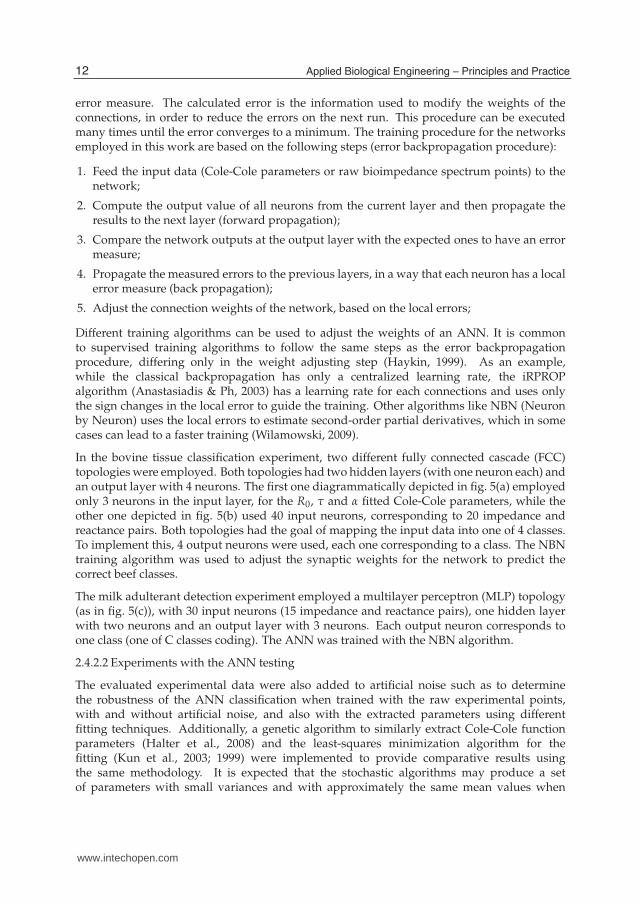
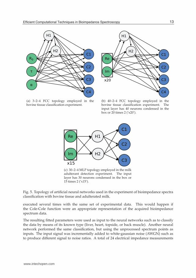
In the bovine tissue classification experiment, two different fully connected cascade (FCC)topologies were employed. Both topologies had two hidden layers (with one neuron each) andan output layer with 4 neurons. The first one diagrammatically depicted in fig. 5(a) employedonly 3 neurons in the input layer, for the R0, τ and α fitted Cole-Cole parameters, while theother one depicted in fig. 5(b) used 40 input neurons, corresponding to 20 impedance andreactance pairs. Both topologies had the goal of mapping the input data into one of 4 classes.To implement this, 4 output neurons were used, each one corresponding to a class. The NBNtraining algorithm was used to adjust the synaptic weights for the network to predict thecorrect beef classes.

The milk adulterant detection experiment employed a multilayer perceptron (MLP) topology(as in fig. 5(c)), with 30 input neurons (15 impedance and reactance pairs), one hidden layerwith two neurons and an output layer with 3 neurons. Each output neuron corresponds toone class (one of C classes coding). The ANN was trained with the NBN algorithm.

2.4.2.2 Experiments with the ANN testing

The evaluated experimental data were also added to artificial noise such as to determinethe robustness of the ANN classification when trained with the raw experimental points,with and without artificial noise, and also with the extracted parameters using differentfitting techniques. Additionally, a genetic algorithm to similarly extract Cole-Cole functionparameters (Halter et al., 2008) and the least-squares minimization algorithm for thefitting (Kun et al., 2003; 1999) were implemented to provide comparative results usingthe same methodology. It is expected that the stochastic algorithms may produce a setof parameters with small variances and with approximately the same mean values when


www.intechopen.com


!

"

#

$

%&

'

(!

("

(a) 3–2–4 FCC topology employed in thebovine tissue classification experiment.

!

"

#

$

%!

%"

&'

()

*"+

(b) 40–2–4 FCC topology employed in thebovine tissue classification experiment. Theinput layer has 40 neurons condensed in thebox or 20 times 2 (’x20’).

!

"#

$%

$&

'%

'&

'()%*(c) 30–2–4 MLP topology employed in the milkadulterant detection experiment. The inputlayer has 30 neurons condensed in the box or15 times 2 (’x15’).

Fig. 5. Topology of artificial neural networks used in the experiment of bioimpedance spectraclassification with bovine tissue and adulterated milk.

executed several times with the same set of experimental data. This would happen ifthe Cole-Cole function were an appropriate representation of the acquired bioimpedancespectrum data.

The resulting fitted parameters were used as input to the neural networks such as to classifythe data by means of its known type (liver, heart, topside, or back muscle). Another neuralnetwork performed the same classification, but using the unprocessed spectrum points asinputs. The input signal was incrementally added to white-gaussian noise (AWGN) such asto produce different signal to noise ratios. A total of 24 electrical impedance measurements


www.intechopen.com


were divided into two sets. The first set is formed by 15 measured spectra and is used for theneural network training, while the second set formed by the remaining 9 measurements wereused for the neural network validation test. Another 11 sets were created with AWGN havingsignal-to-noise ratio (SNR) from 2 to 32 dB with steps of 2 dB, forming the base validation setwhere each spectrum was used more than once to sum a total of 20 spectra in each set. FourANN were created, one for each fitting algorithm and another for the raw spectra. Each neuralnetwork was trained with the spectra from the training set and tested with the validation sets,using the corresponding results from the extracted Cole-Cole parameter output or the rawspectra as input. The neural networks for the use with the testing of fitting algorithms havea 3 − 2 − 4 fully connected cascade (FCC) topology to allow a better generalization in theANN (Wilamowski, 2009), as diagrammatically illustrated in fig. 5, with the 3 input neuronscorresponding to the [R0, τ0, α] parameters and the 4 output neurons corresponding to theconfidence level of each bovine tissue type.

The neural network that uses the set of bioimpedance spectrum points as input with a 40 −2 − 4 FCC topology had the 40 inputs corresponding to the real and imaginary parts of the 20input spectrum points associated with the lowest frequencies in the experimental spectrumwhich would correspond to a maximum frequency of 60 kHz.

One ANN was trained with the parameters fitted by the PSO algorithm using the training set,by exposing the ANN to the sample values associated with the input that corresponds to theextracted Cole-Cole parameters. After that, the neural network performance was measured toclassify the sample type correctly. The rate of correct classifications was calculated by usingthe extracted parameters and also the raw data from 11 spectrum and using the correspondingtrained ANN.

2.4.3 Raw milk evaluation through bioimpedance spectra

In the dairy industry, conductivity measurements are made to test for abnormal milk. This issomehow similar to the process of obtaining a bioimpedance spectrum from a milk sample.However, in conductivity tests the sample is usually interrogated at a single frequencyand the results give false positives and negatives (Belloque et al., 2008). Conductivity,therefore bioimpedance (Piton et al., 1988), and acidity measurements are also used to measuremicrobial contents of the milk, being indirect and rapid methods (Belloque et al., 2008;Hamann & Zecconi, 1998). The drawbacks of these methods are associated with the lack ofsensitivity and specificity. In addition, the conductivity test is also included in screening teststo detect mastitis. Since mastitic milk contains pathogens and spoilage microorganisms, and itis also characterized by an increase in Na+ and Cl− as well as leucocytes (Kitchen, 1981), thismay be indicated by changes in bioimpedance spectrum (Bertemes-Filho, Negri & Paterno,2010) as discussed here, and it would also characterize the analysis of raw milk as of a cellsuspension.

Other changes in the milk, which may not have its causes in a sick animal, could also beindicated by changes in the bioimpedance spectrum, as when the milk has water or hydrogenperoxide, for example, added to it for fraudulent purposes (Bertemes-Filho et al., 2011). Themodulus and phase of the bioimpedance along a frequency range containing more than onefrequency point is therefore an extension of the typical measurement of conductivity in theprocess of milk quality evaluation and is justified by previous published results.


www.intechopen.com


2.4.3.1 Detection of water and hydrogen peroxide in raw milk

Milk may be adulterated by the addition of water, food coloring, conservants and substancesused for the milk thickening, as for example the hydrogen peroxide. The commonest methodof adulterating milk may be the dilution of water and a common method to detect it is bymeasuring its freezing point and use this value to calculate the percentage of the dilutedwater (Belloque et al., 2008). Another indication of water content would be provided bychanges of bioimpedance spectra from the milk. To illustrate it, the bioimpedance spectrafrom raw milk with and without added water and hydrogen peroxide were determined andcompared with each other.

An ANN is subsequently used to classify the milk sample by using the points of thebioimpedance spectrum. For this purpose, samples of raw milk from 27 Holstein cows inlactation were obtained in a local farm. The sample sets were divided into two groups. Thefirst group (A) was used to train the neural network with 16 samples. From this set, 4 sampleswere randomly taken and had distilled water added to them in a volumetric concentration of10%; other 4 samples had hydrogen peroxide added to them in a volumetric concentration of3%. In the second group (B), 11 samples were used for the ANN validation, this is, to test ifthe trained algorithm correctly classifies the samples, that were also equivalently adulterated.Before the measurements, the samples were kept in a refrigerator at a temperature of 4◦C for4 hours.

The ANN used the multilayer perceptron topology of fig.5(c) with 30 neurons correspondingto resistance and reactance input values at 15 different frequency points in the bioimpedancespectrum. The output layer was formed by 3 neurons corresponding to a defined class (rawmilk, milk with water and milk with hydrogen peroxide). If the bioimpedance spectrum of asample containing H2O2 is fed to the ANN, this output neuron must have the largest valueoutput among the other two output neurons.

The ANN was trained using the Neuron by Neuron (NBN) algorithm by using 24 spectra, inwhich 4 samples were adulterated with water and other 4 with H2O2. For the ANN validation,30 milk bioimpedance spectra were measured in a different data set producing another dataset different from the one used in the training. The validation spectra were then separatedinto three different classes associated with the evaluated types of samples and the percentageof correct classifications were calculated.

2.4.3.2 Evaluation of mastitic milk

The bioimpedance spectra of raw milk were acquired in samples from 17 Holstein cows,three of them with mastitis infection. Three milk samples of 100 ml from each animalwere collected and stored in a refrigerator at a temperature of 4◦C. Four hours later, thebioimpedance spectrum from each sample was collected and the material was sent to anaccredited laboratory to characterize the presence of somatic cells and bacteria by using flowcytometry1. Selected samples had the acquired bioimpedance spectrum data points processedand the experimental points and Cole-Cole parameters analyzed and shown for illustrationpurposes of the changes presented in the mastitic and raw milk spectra.

1 The laboratory managed to follow the International Dairy Federation Standards 148:2008 and 196:2004.These standards specify, respectively, methods for the counting of somatic cells and for the quantitativedetermination of bacteriological quality in raw milk.


www.intechopen.com


3. Results and discussion

3.1 Retrieving modulus from phase in experimental bioimpedance spectra

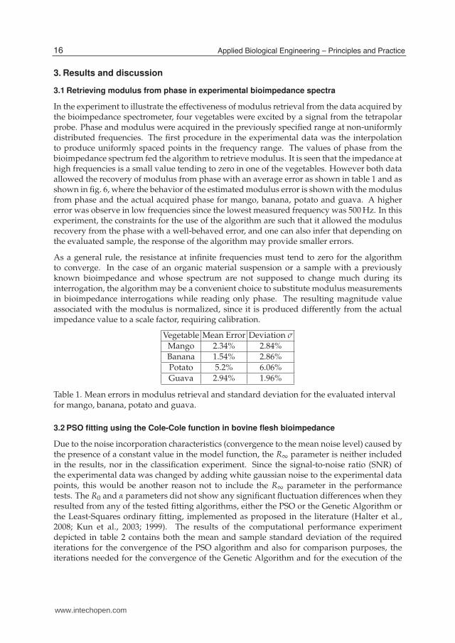
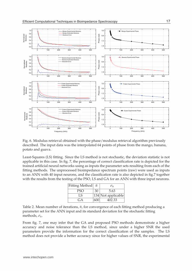
In the experiment to illustrate the effectiveness of modulus retrieval from the data acquired bythe bioimpedance spectrometer, four vegetables were excited by a signal from the tetrapolarprobe. Phase and modulus were acquired in the previously specified range at non-uniformlydistributed frequencies. The first procedure in the experimental data was the interpolationto produce uniformly spaced points in the frequency range. The values of phase from thebioimpedance spectrum fed the algorithm to retrieve modulus. It is seen that the impedance athigh frequencies is a small value tending to zero in one of the vegetables. However both dataallowed the recovery of modulus from phase with an average error as shown in table 1 and asshown in fig. 6, where the behavior of the estimated modulus error is shown with the modulusfrom phase and the actual acquired phase for mango, banana, potato and guava. A highererror was observe in low frequencies since the lowest measured frequency was 500 Hz. In thisexperiment, the constraints for the use of the algorithm are such that it allowed the modulusrecovery from the phase with a well-behaved error, and one can also infer that depending onthe evaluated sample, the response of the algorithm may provide smaller errors.

As a general rule, the resistance at infinite frequencies must tend to zero for the algorithmto converge. In the case of an organic material suspension or a sample with a previouslyknown bioimpedance and whose spectrum are not supposed to change much during itsinterrogation, the algorithm may be a convenient choice to substitute modulus measurementsin bioimpedance interrogations while reading only phase. The resulting magnitude valueassociated with the modulus is normalized, since it is produced differently from the actualimpedance value to a scale factor, requiring calibration.

Vegetable Mean Error Deviation σ

Mango 2.34% 2.84%Banana 1.54% 2.86%Potato 5.2% 6.06%Guava 2.94% 1.96%

Table 1. Mean errors in modulus retrieval and standard deviation for the evaluated intervalfor mango, banana, potato and guava.

3.2 PSO fitting using the Cole-Cole function in bovine flesh bioimpedance

Due to the noise incorporation characteristics (convergence to the mean noise level) caused bythe presence of a constant value in the model function, the R∞ parameter is neither includedin the results, nor in the classification experiment. Since the signal-to-noise ratio (SNR) ofthe experimental data was changed by adding white gaussian noise to the experimental datapoints, this would be another reason not to include the R∞ parameter in the performancetests. The R0 and α parameters did not show any significant fluctuation differences when theyresulted from any of the tested fitting algorithms, either the PSO or the Genetic Algorithm orthe Least-Squares ordinary fitting, implemented as proposed in the literature (Halter et al.,2008; Kun et al., 2003; 1999). The results of the computational performance experimentdepicted in table 2 contains both the mean and sample standard deviation of the requirediterations for the convergence of the PSO algorithm and also for comparison purposes, theiterations needed for the convergence of the Genetic Algorithm and for the execution of the


www.intechopen.com


0 100 200 300 400 500

0,0

0,2

0,4

0,6

0,8

1,0

0 100 200 300 400 500

-1,8

-1,2

-0,6

0,0

0 100 200 300 400 500

0,0

0,2

0,4

0,6

0,8

1,0

0 100 200 300 400 500

-1,8

-1,2

-0,6

0,0

0 100 200 300 400 500

0,0

0,2

0,4

0,6

0,8

1,0

0 100 200 300 400 500

-1,8

-1,2

-0,6

0,0

0 100 200 300 400 500

0,0

0,2

0,4

0,6

0,8

1,0

0 100 200 300 400 500

-1,8

-1,2

-0,6

0,0

Norm

aliz

ed

Modulu

s

Mango Experimental Modulus

Mango Estimated Modulus

Absolute Error

Phase (

rad)

Mango Experimental Phase

Norm

aliz

ed

Modulu

s

Banana Experimental Modulus

Banana Estimated Modulus

Absolute Error

Phase (

rad)

Banana Experimental Phase

Norm

aliz

ed

Modulu

s

Potato Experimental Modulus

Potato Estimated Modulus

Absolute Error

Phase (

rad)

Potato Experimental Phase

Norm

aliz

ed

Modulu

s

Guava Experimental Modulus

Guava Estimated Modulus

Absolute Error

Frequency (kHz)

Phase (

rad)

Frequency (kHz)

Guava Experimental Phase

Fig. 6. Modulus retrieval obtained with the phase/modulus retrieval algorithm previouslydescribed. The input data was the interpolated 64 points of phase from the mango, banana,potato and guava.

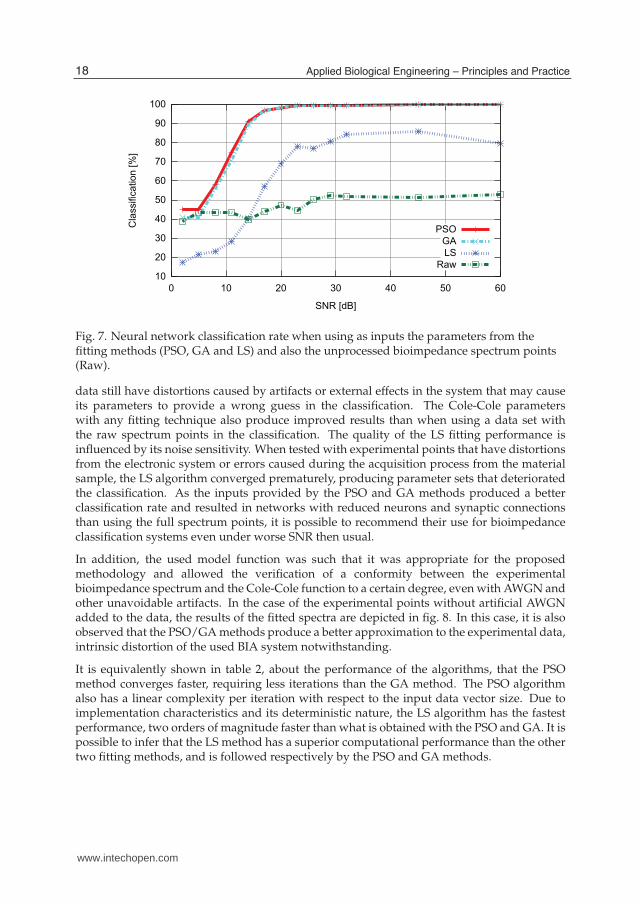
Least-Squares (LS) fitting. Since the LS method is not stochastic, the deviation statistic is notapplicable in this case. In fig. 7, the percentage of correct classification rate is depicted for thetrained artificial neural networks using as inputs the parameter sets resulting from each of thefitting methods. The unprocessed bioimpedance spectrum points (raw) were used as inputsto an ANN with 40 input neurons, and the classification rate is also depicted in fig.7 togetherwith the results from the testing of the PSO, LS and GA for an ANN with three input neurons.

Fitting Method n σn

PSO 30 5.63LS 134 Not applicableGA 600 402.33

Table 2. Mean number of iterations, n, for convergence of each fitting method producing aparameter set for the ANN input and its standard deviation for the stochastic fittingmethods, σn.

From fig. 7, one may infer that the GA and proposed PSO methods demonstrate a higheraccuracy and noise tolerance than the LS method, since under a higher SNR the usedparameters provide the information for the correct classification of the samples. The LSmethod does not provide a better accuracy since for higher values of SNR, the experimental


www.intechopen.com


!

"!

#!

$!

%!

&!

'!

(!

)!

!!

! ! "! #! $! %! &!

*+,--./.0,1.234567

89:45;<7

=8>?@A8:,B

Fig. 7. Neural network classification rate when using as inputs the parameters from thefitting methods (PSO, GA and LS) and also the unprocessed bioimpedance spectrum points(Raw).

data still have distortions caused by artifacts or external effects in the system that may causeits parameters to provide a wrong guess in the classification. The Cole-Cole parameterswith any fitting technique also produce improved results than when using a data set withthe raw spectrum points in the classification. The quality of the LS fitting performance isinfluenced by its noise sensitivity. When tested with experimental points that have distortionsfrom the electronic system or errors caused during the acquisition process from the materialsample, the LS algorithm converged prematurely, producing parameter sets that deterioratedthe classification. As the inputs provided by the PSO and GA methods produced a betterclassification rate and resulted in networks with reduced neurons and synaptic connectionsthan using the full spectrum points, it is possible to recommend their use for bioimpedanceclassification systems even under worse SNR then usual.

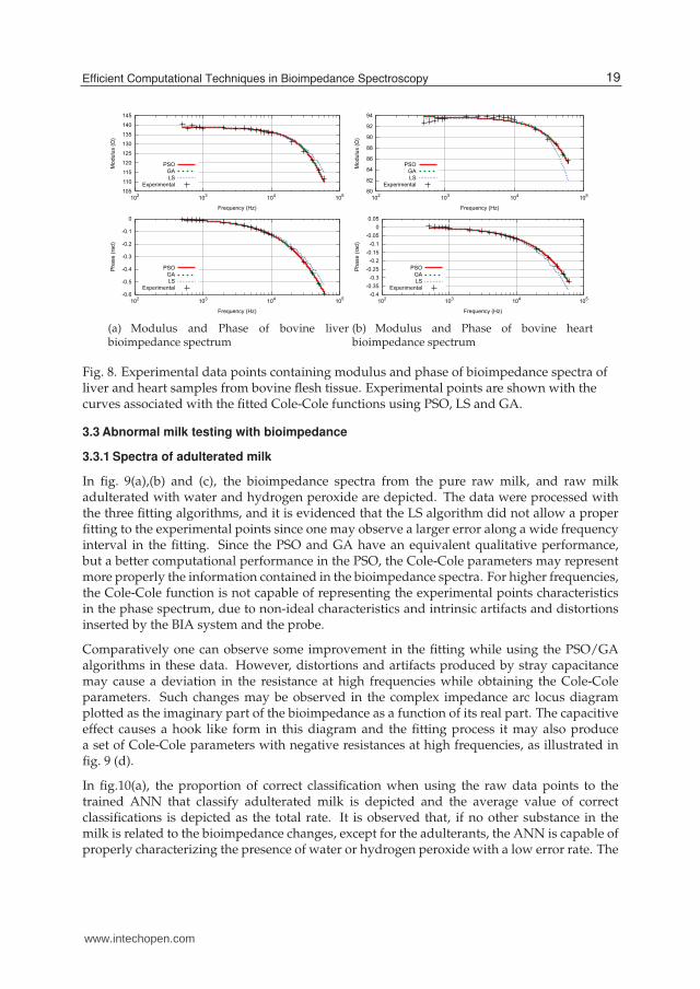
In addition, the used model function was such that it was appropriate for the proposedmethodology and allowed the verification of a conformity between the experimentalbioimpedance spectrum and the Cole-Cole function to a certain degree, even with AWGN andother unavoidable artifacts. In the case of the experimental points without artificial AWGNadded to the data, the results of the fitted spectra are depicted in fig. 8. In this case, it is alsoobserved that the PSO/GA methods produce a better approximation to the experimental data,intrinsic distortion of the used BIA system notwithstanding.

It is equivalently shown in table 2, about the performance of the algorithms, that the PSOmethod converges faster, requiring less iterations than the GA method. The PSO algorithmalso has a linear complexity per iteration with respect to the input data vector size. Due toimplementation characteristics and its deterministic nature, the LS algorithm has the fastestperformance, two orders of magnitude faster than what is obtained with the PSO and GA. It ispossible to infer that the LS method has a superior computational performance than the othertwo fitting methods, and is followed respectively by the PSO and GA methods.


www.intechopen.com


!" ! " #! #" $! $" %! %"

!# !$ !% !"

&'()*)+,-.

/

0123)2456,-78/

9:;<=>:

?@A21BC24DE*

F!GH

F!G"

F!G%

F!G$

F!G#

F!G

!

!# !$ !% !"

9IE+2,-1E(/

0123)2456,-78/

9:;<=>:

?@A21BC24DE*

(a) Modulus and Phase of bovine liverbioimpedance spectrum

!

"

#

$

%!

%"

%#

&!" &!' &!# &!(

)*+,-,./012

3456,5789/0:;2

<=>?@A=

BCD54EF57GH-

I!J#I!J'(I!J'I!J"(I!J"I!J&(I!J&I!J!(

!!J!(

&!" &!' &!# &!(

<KH.5/04H+2

3456,5789/0:;2

<=>?@A=

BCD54EF57GH-

(b) Modulus and Phase of bovine heartbioimpedance spectrum

Fig. 8. Experimental data points containing modulus and phase of bioimpedance spectra ofliver and heart samples from bovine flesh tissue. Experimental points are shown with thecurves associated with the fitted Cole-Cole functions using PSO, LS and GA.

3.3 Abnormal milk testing with bioimpedance

3.3.1 Spectra of adulterated milk

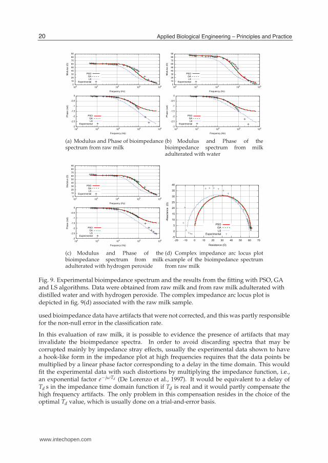
In fig. 9(a),(b) and (c), the bioimpedance spectra from the pure raw milk, and raw milkadulterated with water and hydrogen peroxide are depicted. The data were processed withthe three fitting algorithms, and it is evidenced that the LS algorithm did not allow a properfitting to the experimental points since one may observe a larger error along a wide frequencyinterval in the fitting. Since the PSO and GA have an equivalent qualitative performance,but a better computational performance in the PSO, the Cole-Cole parameters may representmore properly the information contained in the bioimpedance spectra. For higher frequencies,the Cole-Cole function is not capable of representing the experimental points characteristicsin the phase spectrum, due to non-ideal characteristics and intrinsic artifacts and distortionsinserted by the BIA system and the probe.

Comparatively one can observe some improvement in the fitting while using the PSO/GAalgorithms in these data. However, distortions and artifacts produced by stray capacitancemay cause a deviation in the resistance at high frequencies while obtaining the Cole-Coleparameters. Such changes may be observed in the complex impedance arc locus diagramplotted as the imaginary part of the bioimpedance as a function of its real part. The capacitiveeffect causes a hook like form in this diagram and the fitting process it may also producea set of Cole-Cole parameters with negative resistances at high frequencies, as illustrated infig. 9 (d).

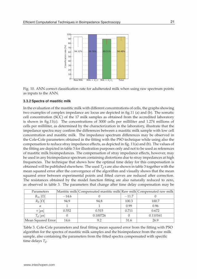
In fig.10(a), the proportion of correct classification when using the raw data points to thetrained ANN that classify adulterated milk is depicted and the average value of correctclassifications is depicted as the total rate. It is observed that, if no other substance in themilk is related to the bioimpedance changes, except for the adulterants, the ANN is capable ofproperly characterizing the presence of water or hydrogen peroxide with a low error rate. The


www.intechopen.com


! " # $ % & ' ( )

! " ! # ! $ ! % ! &

*+,-.-/0123

4567-689:01;<3

=>?@AB>

CDE65FG68HI.

J#

J"K%

J"

J!K%

J!

J K%

! " ! # ! $ ! % ! &

=LI/6015I,3

4567-689:01;<3

=>?@AB>

CDE65FG68HI.

(a) Modulus and Phase of bioimpedancespectrum from raw milk

! " # $ % & ' ( )

! " ! # ! $ ! % ! &

*+,-.-/0123

4567-689:01;<3

=>?@AB>

CDE65FG68HI.

J#

J"K%

J"

J!K%

J!

J K%

! " ! # ! $ ! % ! &

=LI/6015I,3

4567-689:01;<3

=>?@AB>

CDE65FG68HI.

(b) Modulus and Phase of thebioimpedance spectrum from milkadulterated with water

! " # $ % & ' ( )

! " ! # ! $ ! % ! &

*+,-.-/0123

4567-689:01;<3

=>?@AB>

CDE65FG68HI.

J#

J"K%

J"

J!K%

J!

J K%

! " ! # ! $ ! % ! &

=LI/6015I,3

4567-689:01;<3

=>?@AB>

CDE65FG68HI.

(c) Modulus and Phase of thebioimpedance spectrum from milkadulterated with hydrogen peroxide

!

"

!

#"

#!

$"

$!

%"

%!

&"

$" #" " #" $" %" &" !" '" ("

)*+,-+.,*//012

)*343-+.,*/012

56789:6

;<=*>4?*.-+@

(d) Complex impedance arc locus plotexample of the bioimpedance spectrumfrom raw milk

Fig. 9. Experimental bioimpedance spectrum and the results from the fitting with PSO, GAand LS algorithms. Data were obtained from raw milk and from raw milk adulterated withdistilled water and with hydrogen peroxide. The complex impedance arc locus plot isdepicted in fig. 9(d) associated with the raw milk sample.

used bioimpedance data have artifacts that were not corrected, and this was partly responsiblefor the non-null error in the classification rate.

In this evaluation of raw milk, it is possible to evidence the presence of artifacts that mayinvalidate the bioimpedance spectra. In order to avoid discarding spectra that may becorrupted mainly by impedance stray effects, usually the experimental data shown to havea hook-like form in the impedance plot at high frequencies requires that the data points bemultiplied by a linear phase factor corresponding to a delay in the time domain. This wouldfit the experimental data with such distortions by multiplying the impedance function, i.e.,an exponential factor e−jωTd (De Lorenzo et al., 1997). It would be equivalent to a delay ofTd s in the impedance time domain function if Td is real and it would partly compensate thehigh frequency artifacts. The only problem in this compensation resides in the choice of theoptimal Td value, which is usually done on a trial-and-error basis.


www.intechopen.com


Fig. 10. ANN correct classification rate for adulterated milk when using raw spectrum pointsas inputs to the ANN.

3.3.2 Spectra of mastitic milk

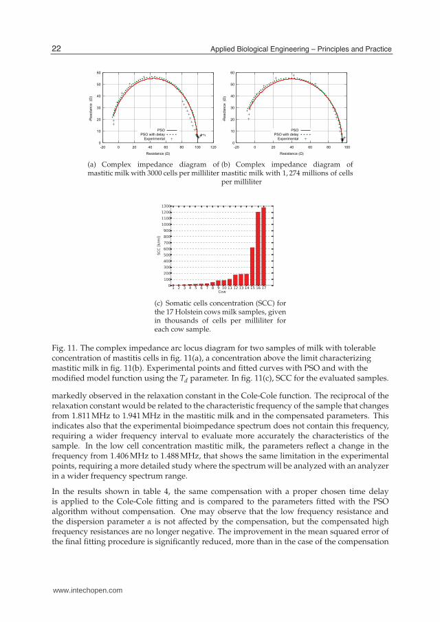
In the evaluation of the mastitic milk with different concentrations of cells, the graphs showingtwo examples of complex impedance arc locus are depicted in fig.11 (a) and (b). The somaticcell concentration (SCC) of the 17 milk samples as obtained from the accredited laboratoryis shown in fig.11(c). The concentrations of 3000 cells per milliliter and 1.274 millions ofcells per milliliter, as determined by the characterization in the laboratory, illustrate that theimpedance spectra may confirm the differences between a mastitic milk sample with low cellconcentration and mastitic milk. The impedance spectrum differences may be observed inthe Cole-Cole parameters obtained in the fitting with the PSO technique while using also thecompensation to reduce stray impedance effects, as depicted in fig. 11(a) and (b). The values ofthe fitting are depicted in table 3 for illustration purposes only and not to be used as referencesof mastitic milk bioimpedances. The compensation of stray impedance effects, however, maybe used in any bioimpedance spectrum containing distortions due to stray impedances at highfrequencies. The technique that shows how the optimal time delay for this compensation isobtained will be published elsewhere. The used Td s are also shown in table 3 together with themean squared error after the convergence of the algorithm and visually shows that the meansquared error between experimental points and fitted curves are reduced after correction.The resistances obtained by the model function fitting are also naturally reduced to zero,as observed in table 3. The parameters that change after time delay compensation may be

Parameters Mastitic milk Compensated mastitic milk Raw milk Compensated raw milkR∞ [Ω] −14.6 0 −11.7 0R0 [Ω] 94.9 94.8 100.3 100.7

α 1 1 0.99 0.96τ [μs] 0.552 0.515 0.711 0.672Td [μs] 0 0.100726 0 0.110161

Mean Squared Error 14.6 9.2 31.6 26.9

Table 3. Cole-Cole parameters and final fitting mean squared error from the fitting with PSOalgorithm for the spectra of mastitic milk samples and the bioimpedance from the raw milksample, also containing the parameters from the fitted spectra compensated with specifictime delays Td.


www.intechopen.com


!

"

#

$

%

&

'" " $ & ( ! !"

')*+,-+.,*//012

)*343-+.,*/012

567567/84-9/:*;+<=>?*@4A*.-+;

(a) Complex impedance diagram ofmastitic milk with 3000 cells per milliliter

!

"

#

$

%

&

'" " $ & ( !

')*+,-+.,*//012

)*343-+.,*/012

567567/84-9/:*;+<=>?*@4A*.-+;

(b) Complex impedance diagram ofmastitic milk with 1, 274 millions of cellsper milliliter

(c) Somatic cells concentration (SCC) forthe 17 Holstein cows milk samples, givenin thousands of cells per milliliter foreach cow sample.

Fig. 11. The complex impedance arc locus diagram for two samples of milk with tolerableconcentration of mastitis cells in fig. 11(a), a concentration above the limit characterizingmastitic milk in fig. 11(b). Experimental points and fitted curves with PSO and with themodified model function using the Td parameter. In fig. 11(c), SCC for the evaluated samples.

markedly observed in the relaxation constant in the Cole-Cole function. The reciprocal of therelaxation constant would be related to the characteristic frequency of the sample that changesfrom 1.811 MHz to 1.941 MHz in the mastitic milk and in the compensated parameters. Thisindicates also that the experimental bioimpedance spectrum does not contain this frequency,requiring a wider frequency interval to evaluate more accurately the characteristics of thesample. In the low cell concentration mastitic milk, the parameters reflect a change in thefrequency from 1.406 MHz to 1.488 MHz, that shows the same limitation in the experimentalpoints, requiring a more detailed study where the spectrum will be analyzed with an analyzerin a wider frequency spectrum range.

In the results shown in table 4, the same compensation with a proper chosen time delayis applied to the Cole-Cole fitting and is compared to the parameters fitted with the PSOalgorithm without compensation. One may observe that the low frequency resistance andthe dispersion parameter α is not affected by the compensation, but the compensated highfrequency resistances are no longer negative. The improvement in the mean squared error ofthe final fitting procedure is significantly reduced, more than in the case of the compensation


www.intechopen.com


!"

#

"

#

!"

!#

$"

$#

%"

%#

&"

$" !" " !" $" %" &" #" '" ("

)*+,-+.,*//012

)*343-+.,*/012

567567/84-9/:*;+<=>?*@4A*.-+;

(a) Complex impedance diagram of rawmilk

!"

"

!"

#"

$"

%"

&"

' "

#" " #" %" ' " (" !""

)*+,-+.,*//012

)*343-+.,*/012

567567/84-9/:*;+<=>?*@4A*.-+;

(b) Complex impedance diagram of milkwith water

!

"

"!

#

#!

$

$!

%" " # $ & ! ' (

%)*+,-+.,*//012

)*343-+.,*/012

567567/84-9/:*;+<=>?*@4A*.-+;

(c) Complex impedance diagram of milkwith hydrogen peroxide

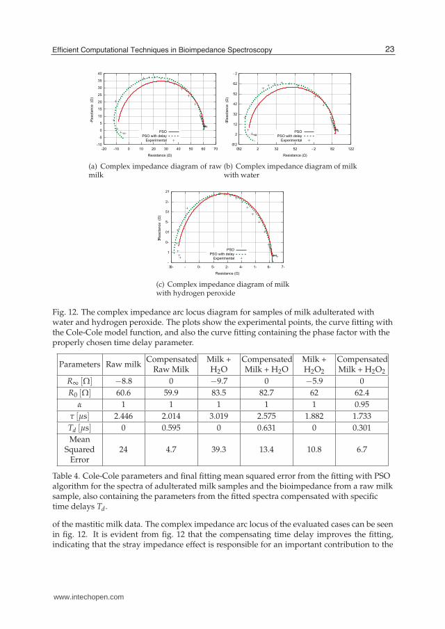
Fig. 12. The complex impedance arc locus diagram for samples of milk adulterated withwater and hydrogen peroxide. The plots show the experimental points, the curve fitting withthe Cole-Cole model function, and also the curve fitting containing the phase factor with theproperly chosen time delay parameter.

Parameters Raw milkCompensated

Raw MilkMilk +H2O

CompensatedMilk + H2O

Milk +H2O2

CompensatedMilk + H2O2

R∞ [Ω] −8.8 0 −9.7 0 −5.9 0R0 [Ω] 60.6 59.9 83.5 82.7 62 62.4

α 1 1 1 1 1 0.95τ [μs] 2.446 2.014 3.019 2.575 1.882 1.733Td [μs] 0 0.595 0 0.631 0 0.301Mean

SquaredError

24 4.7 39.3 13.4 10.8 6.7

Table 4. Cole-Cole parameters and final fitting mean squared error from the fitting with PSOalgorithm for the spectra of adulterated milk samples and the bioimpedance from a raw milksample, also containing the parameters from the fitted spectra compensated with specifictime delays Td.

of the mastitic milk data. The complex impedance arc locus of the evaluated cases can be seenin fig. 12. It is evident from fig. 12 that the compensating time delay improves the fitting,indicating that the stray impedance effect is responsible for an important contribution to the


www.intechopen.com


hook-like behavior of the complex impedance arc locus. Observing the dispersion parameterα, it is usually close to unity in every sample, compensated or not. This is an indicationthat the milk may be modeled by a single pole function with fitting errors of the same orderof magnitude as shown in table 4 and 3. Differently from the mastitic milk analysis, thereciprocal of the relaxation constant is in the experimental frequency interval obtained withthe BIA system. The characteristic frequency of the samples in the raw milk changes from408 kHz to 496 kHz after compensation. Equivalently for adulterated milk with water andhydrogen peroxide, the changes occur from 331 kHz to 388 kHz and from 531 kHz to 577 kHz,respectively. These variations indicate an increase in the compensated characteristic frequencywhen the stray effects are compensated this way.

4. Conclusion

The authors report the use of computational intelligence and also well known digital signalprocessing algorithms in bioimpedance spectroscopy. The BIA analysis of data obtainedfrom a custom made spectrometer were processed with a modulus retrieval algorithm fromphase of bioimpedance spectra of vegetables showing the feasibility of using this specificand well known algorithm in a practical case. This would also allow the BIA systemhardware to be simplified. In this case, since only the phase of the bioimpedance is goingto be acquired to obtain the complete modulus of the bioimpedance spectrum, the involvedelectronic circuitry, as expected, may be reduced and the instrumentation amplifiers tomeasure modulus would be unnecessary. This would pave the way to embed algorithms in amuch more simplified electronics for bioimpedance systems designed for specific applicationsas in the characterization of fruits, for example.

The bioimpedance data may also be processed with computational intelligence techniques.The authors improved already known techniques to fit experimental bioimpedance spectrumdata to a specific model function. This is common practice in bioimpedance spectroscopyand is already implemented in commercial systems, however they do not use the techniquesproposed here, only the least-squares algorithms, but no other more elaborate algorithms,like evolutionary techniques and particle-swarm optimization procedures. It is shown thatthe PSO technique has advantages over the already proposed procedures. The comparison ofsuch techniques was implemented and artificial neural networks were used for the specificpurpose of comparing them. The use of an Artificial Neural Network that receives asinput the parameters produced by the fitting illustrates that different techniques, specificallythe least-square fitting, simply would not be capable of allowing the identification of thecorrect tissue or the sample experimentally evaluated. The genetic algorithm and theparticle-swarm optimization were capable of allowing the correct classification of the sampleswith experimental data added to noise in a much better proportion than the least-squaresalgorithm. Considering that the number of iterations in the PSO is much less than the geneticalgorithm, and since they provide the same qualitative results in terms of classification, thePSO shows a superiority with respect to performance. The arithmetic complexity of the PSOis also an important characteristic that could facilitate embedded implementations.

Still in the dairy food applications, the idea of using bioimpedance to classify milk withthe previously described techniques was also illustrated. Milk with different concentrationsof mastitis cells were evaluated and the differences in the phase and modulus of thebioimpedance spectrum are noticed. However, the selectivity of the BIA system couldnot be demonstrated, and this would force one to use other additional sensing systems to


www.intechopen.com


evidence the interesting characteristic. During the evaluation of adulterated milk with typicaladulterants, like water and hydrogen peroxide, the information would be present in thebioimpedance spectrum, but an identification of the exact adulterant or its quantity wouldrequire other sensing systems.

The experimental data produced with the milk evaluation have also other characteristicsnot related to the sample itself, but to the instrumentation and also to reactions occurringbetween the sample and the electrode. The hook like figure in the complex plane arc locusin the milk measurements demonstrate the effect. Such a behavior may be considered dueto adsorption in the impedance electrode in some types of samples. However, the hook-likecharacteristic of the spectrum may be due to impedance stray effects, either from the cables,electrodes or the electronic circuitry. This may be corrected in some cases with a change inthe model, by considering the effect of a phase corresponding to a complex exponential inthe model function. The optimal values were determined for the correction and the errorin the fitting was significantly reduced in those sets of data. Specifically in the raw mastiticand adulterated milk, the Cole-Cole parameters were compared and the fitting algorithms areonce again shown to be efficient in illustrating the computational power of the techniques inbioimpedance spectroscopy.

5. Future directions

The idea of determining efficient and simple algorithms to process bioimpedance spectra isa topic that may allow the implementation of sophisticated algorithms in embedded systemsand could also improve the quality of the analysis produced by simple equipment. One canmention that in the case of the phase/modulus retrieval algorithms, since the technique isbased on the use of the well-known fast-Fourier transform algorithm, it would be naturalto implement it in embedded systems. However, the applications could not be restricted tosuch systems, since the use of the proposed algorithms may help improve the bioimpedancespectrum analysis while correcting experimental data and retrieving the more convenientinformation from the improved fitting algorithms. The methodology that uses artificialneural networks to evaluate the performance of the algorithms could also be used in systemsthat require automated analysis of bioimpedance spectra, as in an industrial environment tocharacterize samples of milk or beef, for example.

As a direction to the future research efforts, a final goal for the use of such algorithms wouldbe their implementation in reconfigurable hardware, more specifically, in field-programmablegate arrays (FPGA). Commercial systems already use such technologies, like the FPGAin bioimpedance spectrometers (Nacke et al., 2011). Therefore the evaluated techniquesare suggested to be implemented in hardware, since the particle swarm optimizationalgorithms would be a good choice for this purpose. The arithmetic operations in theparticle-swarm optimization update step requires only random number generation, and aseries of summations and multiplications. In the phase/modulus retrieval algorithm case, theFFT could also be easily instantiated from the core provided by the FPGA company.

6. Acknowledgements

The authors gratefully acknowledge the experimental data collected by Rogerio MartinsPereira, Rodrigo Stiz and Guilherme Martignago Zilli as students supervised in theLaboratories of the Santa Catarina State University in Joinville City.


www.intechopen.com


7. References

Aberg, P., Nicander, I., Hansson, J., Geladi, P., Holmgren, U. & Ollmar, S. (2004). Skin canceridentification using multifrequency electrical impedance - a potential screening tool,IEEE Transactions on Biomedical Engineering 51(12): 2097–2102.

Anastasiadis, A. D. & Ph, U. U. (2003). An efficient improvement of the RPROP algorithm,In Proceedings of the First International Workshop on Artificial Neural Networks in PatternRecognition.

Barsoukov, E. & Macdonald, J. R. (eds) (2005). Impedance spectroscopy: theory, experiment andapplications, 2 edn, Wiley, New York.

Belloque, J., Chicon, R. & Recio, I. (2008). Milk Processing and Quality Management, 1 edn,Wiley-Blackwell, West Sussex, United Kingdom.

Bertemes-Filho, P. (2002). Tissue Characterisation using an Impedance Spectroscopy Probe, PhDThesis, The University of Sheffield, UK.

Bertemes-Filho, P., Negri, L. H. & Paterno, A. S. (2010). Mastitis characterization of bovinemilk using electrical impedance spectroscopy, Congresso Brasileiro de EngenhariaBiomédica (CBEB) – Biomedical Engineering Brazilian Congress, pp. 1351–1353.

Bertemes-Filho, P., Negri, L. & Paterno, A. (2011). Detection of bovine milk adulterants usingbioimpedance measurements and artificial neural network, in Ákos Jobbágy (ed.), 5thEuropean Conference of the International Federation for Medical and Biological Engineering,Vol. 37 of IFMBE Proceedings, Springer, pp. 1275–1278.

Bertemes-Filho, P., Paterno, A. S. & Pereira, R. M. (2009). Multichannel bipolar current sourceused in electrical impedance spectroscopy: Preliminary results, in O. Dössel, W. C.Schlegel & R. Magjarevic (eds), World Congress on Medical Physics and BiomedicalEngineering, September 7 - 12, 2009, Munich, Germany, Vol. 25/7 of IFMBE Proceedings,Springer Berlin Heidelberg, pp. 657–660.URL: http://dx.doi.org/10.1007/978-3-642-03885-3_182

Bertemes-Filho, P., Valicheski, R., Pereira, R. M. & Paterno, A. S. (2010). Bioelectricalimpedance analysis for bovine milk: Preliminary results, Journal of Physics: ConferenceSeries 224(1): 012133.URL: http://stacks.iop.org/1742-6596/224/i=1/a=012133

Brown, B. H. (2003). Electrical impedance tomography (EIE): a review, J. Med. Eng. Technol.3: 97–108.

Cole, K. S. (1940). Permeability and impermeability of cell membranes for ions, Cold SpringHarb. Symp. Quant. Biol. 8: 110.

Cole, K. S. (1968). Membranes, Ions and Impulses: A Chapter of Classical Biophysics, BiophysicsSeries, first edn, University of California Press.

Cole, K. S. & Cole, R. H. (1941). Dispersion and Absorption in Dielectrics I. AlternatingCurrent Characteristics, The Journal of Chemical Physics 9(4): 341–351.URL: http://link.aip.org/link/doi/10.1063/1.1750906

Cybenko, G. (1989). Approximation by superpositions of a sigmoidal function, Mathematics ofControl, Signals, and Systems (MCSS) 2: 303–314.

De Lorenzo, A., Andreoli, A., Matthie, J. & Withers, P. (1997). Predicting body cell mass withbioimpedance by using theoretical methods: a technological review, Journal of AppliedPhysiology 82(5): 1542–1558. URL: http://jap.physiology.org/content/82/5/1542.abstract

Fuoss, R. M. & Kirkwood, J. G. (1941). Electrical properties of solids. viii. dipole momentsin polyvinyl chloride-diphenyl systems*, Journal of the American Chemical Society63(2): 385–394. URL: http://pubs.acs.org/doi/abs/10.1021/ja01847a013


www.intechopen.com


Gorban, A. (1998). Approximation of continuous functions of several variables by anarbitrary nonlinear continuous function of one variable, linear functions, and theirsuperpositions, Applied Mathematics Letters 11(3): 45 – 49.URL: http://www.sciencedirect.com/science/article/pii/S0893965998000329

Grimnes, S. & Martinsen, O. G. (2008). Bioimpedance & Bioelectricity BASICS, 2 edn, AcademicPress.

Halter, R. J., Hartov, A., Paulsen, K. D., Schned, A. & Heaney, J. (2008). Genetic andleast squares algorithms for estimating spectral eis parameters of prostatic tissues,Physiological Measurement 29(6): S111.URL: http://stacks.iop.org/0967-3334/29/i=6/a=S10

Hamann, J. & Zecconi, A. (1998). Bulletin 334, Evaluation of the Electrical Conductivity of Milk asa Mastitis Indicator, International Dairy Federation, pp. 1–23.

Hassan, R., Cohanim, B., Weck, O. D. & Venter, G. (2005). A comparison of particleswarm optimization and the genetic algorithm, 46th AIAA/ASME/ASCE/AHS/ASCStructures, Structural Dynamics, and Materials Conference, pp. 1–13.

Hayes, M., Lin, J. S. & Oppenheim, A. V. (1980). Signal Reconstruction from Phase orMagnitude, IEEE Transactions on Acoustics, Speech and Signal Processing 28(6): 672–680.URL: http://dx.doi.org/10.1109/TASSP.1980.1163463

Haykin, S. (1999). Neural Networks, Prentice-Hall, New Jersey.Holder, D. S. (2004). Electrical impedance tomography: methods, history and applications, 1st edn,

Taylor and Francis, New York.Kitchen, B. J. (1981). Bovine mastitis: milk compositional changes and related diagnostic tests,

Journal of Dairy Research 48(01): 167–188.URL: http://dx.doi.org/10.1017/S0022029900021580

Kronig, R. D. L. (1929). The theory of dispersion of x-rays, Journal of the Optical Society ofAmerica 12(6): 547.URL: http://dx.doi.org/10.1364/JOSA.12.000547

Kun, S., Ristic, B., Peura, R. A. & Dunn, R. M. (2003). Algorithm for tissue ischemiaestimation based on electrical impedance spectroscopy, IEEE Transactions onBiomedical Engineering 50(12): 1352–9.

Kun, S., Ristic, B., Peura, R. & Dunn, R. (1999). Real-time extraction of tissue impedance modelparameters for electrical impedance spectrometer, Medical and Biological Engineeringand Computing 37: 428–432.URL: http://dx.doi.org/10.1007/BF02513325

Kyle, U. G., Bosaeus, I., Lorenzo, A. D. D., Deurenberg, P., Elia, M., Gómez, J. M., Heitmann,B. L., Kent-Smith, L., Melchior, J.-C., Pirlich, M., Scharfetter, H., Schols, A. M. &Pichard, C. (2004). Bioelectrical impedance analysis: part i. Review of principles andmethods, Clinical Nutrition 23(5): 1226.

Nacke, T., Barthel, A., Beckmann, D., Pliquett, U., Friedrich, J., Peyerl, P., Helbig,M. & Sachs, J. (2011). Messsystem für die impedanzspektroskopischebreitband-prozessmesstechnik – broadband impedance spectrometer for processinstrumentation, Technisches Messen 78(1): 3–14.URL: http://www.oldenbourg-link.com/doi/abs/10.1524/teme.2011.0077

Negri, L. H., Bertemes-Filho, P. & Paterno, A. S. (2010). Extração dos parâmetros dafunção de Cole-Cole utilizando otimização por enxame de partículas, XXII CongressoBrasileiro de Engenharia Biomédica (CBEB) – Biomedical Engineering Brazilian Congress,pp. 928–931.


www.intechopen.com


Nordbotten, B. J., Tronstad, C., Ørjan G Martinsen & Grimnes, S. (2011). Evaluationof algorithms for calculating bioimpedance phase angle values from measuredwhole-body impedance modulus, Physiological Measurement 32(7): 755.URL: http://stacks.iop.org/0967-3334/32/i=7/a=S03

Paterno, A. S. & Hoffmann, M. (2008). Reconstrução de sinais em espectroscopia debioimpedância elétrica, XXI Congresso Brasileiro de Engenharia Biomédica (CBEB) –Biomedical Engineering Brazilian Congress, pp. 1–4.

Paterno, A., Stiz, R. & Bertemes-Filho, P. (2009). Frequency-domain reconstruction ofsignals in electrical bioimpedance spectroscopy, Medical and Biological Engineering andComputing 47: 1093–1102.URL: http://dx.doi.org/10.1007/s11517-009-0533-1

Piton, C., Dasen, A. & Bardoux, I. (1988). Evaluation de la mesure d’impédance commetechnique rapide d’appréciation de la qualité bactériologique du lait cru, Lait68(4): 467–484.URL: http://dx.doi.org/10.1051/lait:1988430

Proakis, J. G. & Manolakis, D. K. (2006). Digital Signal Processing, 4 edn, Prentice Hall.Quartieri, T. & Oppenheim, A. V. (1981). Iterative techniques for minimum phase signal

reconstruction from phase or magnitude, IEEE Transactions on Acoustics, Speech andSignal Processing 29(6): 1187–1193.URL: http://dx.doi.org/10.1109/TASSP.1981.1163714

Riu, P. J. & Lapaz, C. (1999). Practical limits of the Kramers-Kronig relationships appliedto experimental bioimpedance data, Annals of the New York Academy of Sciences873(1): 374–380.URL: http://dx.doi.org/10.1111/j.1749-6632.1999.tb09486.x

Siegelmann, H. T. & Sontag, E. D. (1991). Turing computability with neural nets, AppliedMathematics Letters 4(6): 77 – 80.URL: http://www.sciencedirect.com/science/article/pii/089396599190080F

Stiz, R. A., Bertemes, P., Ramos, A. & Vincence, V. C. (2009). Wide band Howland bipolarcurrent source using AGC amplifier, IEEE Latin America Transactions 7(5): 514–518.

Waterworth, A. R. (2000). Data Analysis Techniques of Measured Biological Impedance, Phd Thesis,The University of Sheffield, UK.

Wilamowski, B. M. (2009). Neural network architectures and learning algorithms, IEEEIndustrial Electronics Magazine 3: 56–63.

Xiaohui, H., Yuhui, S. & Eberhart, R. (2004). Congress on Evolutionary Computation, 2004 –CEC2004, Vol. 1, IEEE, pp. 90–97.URL: http://ieeexplore.ieee.org/xpl/freeabs_all.jsp?arnumber=1330842


www.intechopen.com

Applied Biological Engineering - Principles and PracticeEdited by Dr. Ganesh R. Naik

ISBN 978-953-51-0412-4Hard cover, 662 pagesPublisher InTechPublished online 23, March, 2012Published in print edition March, 2012

InTech EuropeUniversity Campus STeP Ri Slavka Krautzeka 83/A 51000 Rijeka, Croatia Phone: +385 (51) 770 447 Fax: +385 (51) 686 166www.intechopen.com

InTech ChinaUnit 405, Office Block, Hotel Equatorial Shanghai No.65, Yan An Road (West), Shanghai, 200040, China

Phone: +86-21-62489820 Fax: +86-21-62489821

Biological engineering is a field of engineering in which the emphasis is on life and life-sustaining systems.Biological engineering is an emerging discipline that encompasses engineering theory and practice connectedto and derived from the science of biology. The most important trend in biological engineering is the dynamicrange of scales at which biotechnology is now able to integrate with biological processes. An explosion inmicro/nanoscale technology is allowing the manufacture of nanoparticles for drug delivery into cells,miniaturized implantable microsensors for medical diagnostics, and micro-engineered robots for on-boardtissue repairs. This book aims to provide an updated overview of the recent developments in biologicalengineering from diverse aspects and various applications in clinical and experimental research.

How to referenceIn order to correctly reference this scholarly work, feel free to copy and paste the following:

Aleksander Paterno, Lucas Hermann Negri and Pedro Bertemes-Filho (2012). Efficient ComputationalTechniques in Bioimpedance Spectroscopy, Applied Biological Engineering - Principles and Practice, Dr.Ganesh R. Naik (Ed.), ISBN: 978-953-51-0412-4, InTech, Available from:http://www.intechopen.com/books/applied-biological-engineering-principles-and-practice/efficient-computational-techniques-in-bioimpedance-spectroscopy

© 2012 The Author(s). Licensee IntechOpen. This is an open access articledistributed under the terms of the Creative Commons Attribution 3.0License, which permits unrestricted use, distribution, and reproduction inany medium, provided the original work is properly cited.

http://creativecommons.org/licenses/by/3.0

Documents

Efficient Computational Techniques in Bioimpedance