Efficiency Wage and Union Effects inLabor Demand and Wage Structure in Mexico:

An Application of Quantile Analysis

William F. MaloneyThe World Bank

Eduardo Pontual Ribeiro*

Universidade Federal do Rio Grande do Sul

April 17, 1999

Abstract: Using very detailed firm level data from Mexico, this paper uses quantileanalysis to study the demand for two classes of labor and the determinants of theirwages. Unions appear to have a strong positive impact on the quantity of unskilledlabor employed but none on wages except for the 10th (lowest) quantile of unskilledworkers. This suggests an extreme example of “efficient bargaining” rather than morecommon “monopoly union” behavior and that wage objectives are limited tomaintaining a floor for poorly paid workers. Very significant efficiency wage effectsare identified both in labor demand and in the wage equations suggesting that even inthe absence of minimum wages or union power, substantial segmentation of the laborforce will remain in LDCs. The paper offers the first use of quantile analysis in firmlevel analysis of labor demand and the first use of correct standard errors in 2SLSquantiles.

* We thank Carlos Arango, Omar Arias, Gustavo Gonzaga, Daniel Hamermesh and Lyn Squire for helpfulcomments and to Tania Gomez for vital assistance. We are also grateful to the Mexican National Institute ofStatistics, Geography and Information (INEGI) for the use of the data. INEGI is in no way responsible of anyincorrect manipulation of the data or erroneous conclusions drawn from it. The views expressed here are those ofthe authors only, and should not be associated with the World Bank and its member countries. Contacts:wmaloney@worldbank.org, ribeiro@vortex.ufrgs.br

1

I. Introduction.

The evidence to date suggests that both union power and efficiency wage behavior may

have large effects on the structure and dynamics of labor markets. The literature documenting their

effect on wages, in particular, is vast. However, as Blanchflower et. al. (1991) note, the impact on

employment of unions has received relatively little study, and that of efficiency wages has attracted

even less. Further, as Nickell and Wadhwani (1991) argue, the existence of both phenomena

simultaneously complicates efforts to distinguish between competing models of union behavior.1

Their work and that of Hendricks and Kahn (1991) are among the very few that analyze

employment determination in the presence of efficiency wages and two types of union bargaining: the

“right to manage” (RTM) or “monopoly union” type where unions attempt to set the wage but let

firms choose the level of employment, and the “efficient bargaining” (EB) type where unions bargain

over both (Oswald 1991 and Layard and Nickell 1990). Using a large panel from the UK

manufacturing sector, Nickell and Wadhwani find no evidence of union influence on employment and

mixed evidence of efficiency wage effects. Hendricks and Kahn find EB effects in their study of the

demand for police in the US.

This paper builds on this work in two ways. First, it approaches these issues using quantile

analysis that more completely characterize the distributions of wages and labor demanded than can

be done using the conditional mean based linear regression approaches (OLS, 2SLS) that are

standard. Despite assumptions of identical agents, in fact the samples may show substantial

heterogeneity and large differences in the impacts of regressors across quantiles. For example, union

1 For discussions of the theory of efficiency wages see Stiglitz (1974), Krueger and Summers (1988), Phelps (1994)and Weiss (1990). For a review of the literature on union impacts, see Lewis (1986).

2

power might be expected to impinge more strongly among those who receive a relatively high wage

given their human capital. But, alternatively, unions may put a floor under the wage such that

workers whose productivity is very low given their nominal human capital and leave the rest of the

wage distribution market determined. Efficiency wage effects would probably also be expected to

be most prevalent among those paid “above the market” given their human capital. The results show

the power of this technique to uncover differences that would ordinarily go undetected. The paper

offers the first use of quantile analysis in firm level analysis of labor demand and the first use of

correct standard errors in two stage least square quantiles.

Second, it analyses Mexico, a country with unique institutional, economic and political

characteristics that make it an important case study to add to the literature for two reasons. First, we

may observe union behavior that, although theoretically plausible is contrary to that commonly found.

The manufacturing sector studied here is heavily unionized: 18% of firms have no union

representation, and the rest have a median unionization rate of 70%. However, the massive Labor

Congress (CT) which embraces the Confederation of Mexican Workers (CTM), the Revolutionary

Federation of Workers and Peasants (CROC), the Federation of Government Workers (FSTSE)

and roughly 38 other labor organizations has had a longstanding and close relationship with the

governing Revolutionary Institutional Party (PRI). Particularly since 1987 with the inception of the

Pacto Social- a joint agreement of labor, business and the government to promote price stability-

unions have closely coordinated wage demands with national stabilization objectives. This has made

possible extreme downward flexibility of wages during recent crises and may have curtailed union

3

power along this dimension.2 In addition, it can be argued that in the absence of unemployment

insurance, employment enters more heavily in union objective functions than in the industrialized

countries. The particular constraints and elements of union utility may give rise to EB outcomes with

implications for the structure of wages, and the overall level of employment distinct from those

generally anticipated. It also may permit a test of the assertion (see Nickell and Wadhwani, Layard

and Nickell among others) that the wage-employment relation may slope upward.

Second, the Mexican labor market is well suited to testing for efficiency wage effects.

Though a longstanding literature explains dualistic LDC labor markets by government or union

interference in the wage setting process,3 Mexico’s minimum wage was not binding in the period we

study (Bell 1997), and if unions focus primarily on employment, then the wage structure and

whatever dualism is observed may be emerging endogenously through efficiency wage effects. The

existence of a large non-unionized sector permits isolating such effects whose manifestations can

sometimes be indistinguishable from the outcomes of union bargaining. Further, since the Mexican

Constitution prohibits firing of workers except in extreme circumstances we are arguably testing for

one particular variety of efficiency effect arising from the prevention of turnover (Stiglitz 1974).

The data set we work with is exceptionally rich. It permits conditioning on numerous

dimensions of firm heterogeneity as well as offering some that may conceivably be associated with

efficiency wage effects. It provides evidence on the dynamics of unionized firms and their behavior in

the use of three inputs: unskilled and skilled labor and, to a lesser degree, capital. Disaggregating

2 Though in November of 1997, the New Union of Workers (UNT, .7-1.5 million workers) split from the CTMlargely over what was perceived to be excessive responsiveness to government initiatives, across the periodanalyzed here some analysts have seen a decline in union influence both within the PRI and overall. Thisdiscussion partly based on Collier and Collier (1991) and Brooks and Cason (1998).

4

labor promises an improvement over the vast majority of efficiency bargain papers as we may avoid

a composition bias in the demand for labor due, for example, to the substitutability of types of

workers. Further, we can go beyond the standard (static) labor demand literature with worker types

(e.g. Hamermesh, 1993 and references therein)4 that has not allowed for the possibility of

employment decisions occurring along a contract curve as in the EB solutions instead of the standard

labor demand curve.

The paper is organized as follows. The following section presents the theoretical background

and the testable implications. The third section discusses quantile analysis. The fourth presents the

data set used in the paper and the fifth the empirical results. The last section concludes with a

summary of results.

IIa. Analytics: (Overview)

Efficiency Wages:

The extensive literature on efficiency wages provides a rationale for firms to voluntarily pay

wages above the market clearing level. One common variant of these models arises from the

difficulty of monitoring individual workers and the lack of any penalty from being caught “shirking” -

any activity, or lack thereof, that might be detrimental to the firm. If wages are market clearing, a

worker fired for shirking can simply get another job at the same wage. However, if all firms pay

higher than market clearing wages, unemployment will be created in the economy that creates a

3 See, for example, Harris and Todaro(1970) See Esfahani and Salehi Isfahani (1989) as an example of modelingLDC dualism in an efficiency wage context.4 Hamermesh also points out the clear advantages of using microdata and the dearth of such studies.

5

disincentive to being laid off and hence to shirking. 5

Since, in many Latin American countries, workers can be fired only with difficulty, the

“turnover” variant of efficiency wage models is probably more appropriate: firms must invest

resources in workers when they are hired, perhaps through training or through the process of

recruitment, that will be lost if the worker leaves. Hence, it is worthwhile for firms to pay higher

wages and raise the opportunity cost of leaving.

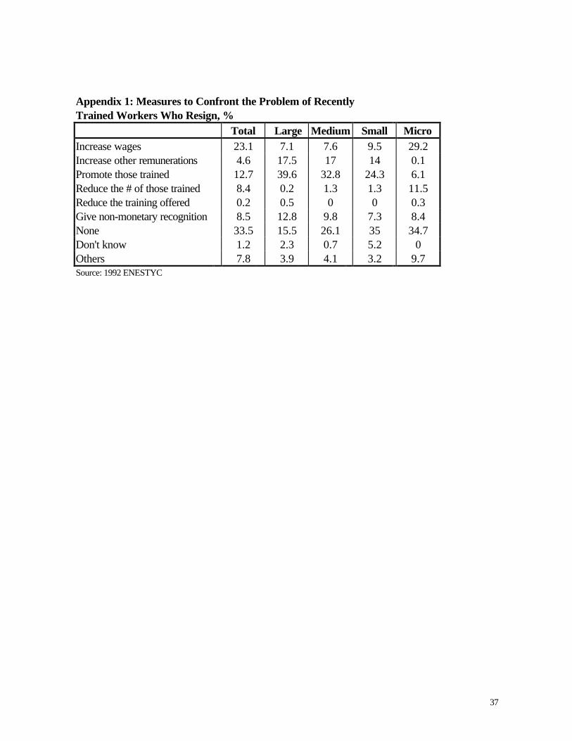
Interviews with Mexican entrepreneurs in the survey used here support this view. Roughly

30% stated that the resignation of recently trained workers was a problem. This is almost certainly

an understatement for two reasons. First, “recently” may not capture the relevant period of return on

the investment in the worker. Second, if the firm is already paying the optimal efficiency wage to

prevent workers from leaving, it will not report excessive turnover as a problem. Of those reporting

frequent resignations after training, 58% do something to raise the total well-being of the worker after

training, 28% raise remuneration without promoting the worker, and 40% take measures that

increases the wage of the worker, including promotions (see Appendix I).

The efficiency wage argument is particularly compelling in LDCs where firms may absorb a

larger share of education costs due to poorly functioning education systems. Thus, firms will be very

concerned about preventing workers they train from moving to another firm. In addition, in countries

where self-employment (formal or informal) are considered desirable destinations, it is possible that

workers enter formal salaried work to accumulate skills and financial capital, and then quit to open

5 As Marquez and Ros (1990) noted, and has been confirmed by later studies, wages of similar workers rise withfirm size, much as they do in industrialized countries. Further, Marquez (1990), Abuhadba and Romaguera (1993)and Schaffner (1998) find efficiency wage effects in the patterns of wage differentials that are strong and highlycorrelated among Chile, Venezuela, and Brazil and the U.S.. This suggests that the conditional wage dispersion(wages adjusted for human capital) and rigidities may be emerging endogenously and are not due to either

6

their own business.

Both theories imply that the offers workers can get outside the firm (the outside wage), as

well as the probability of being able to get a job at that wage (the hiring rate) should be important to

determining the wage that is set in the firm, as well as to the quantity of labor hired.

Union Bargaining.6

The most common view postulates that unions maximize utility, which may be a function of

both the wage received by union members and the level of employment, subject to a constraint

representing combinations of the two that firms are willing to pay, the labor demand curve. In the

“Right to Manage” view unions would identify the level of the wage that maximizes their utility, and

firms simply set the level of employment.

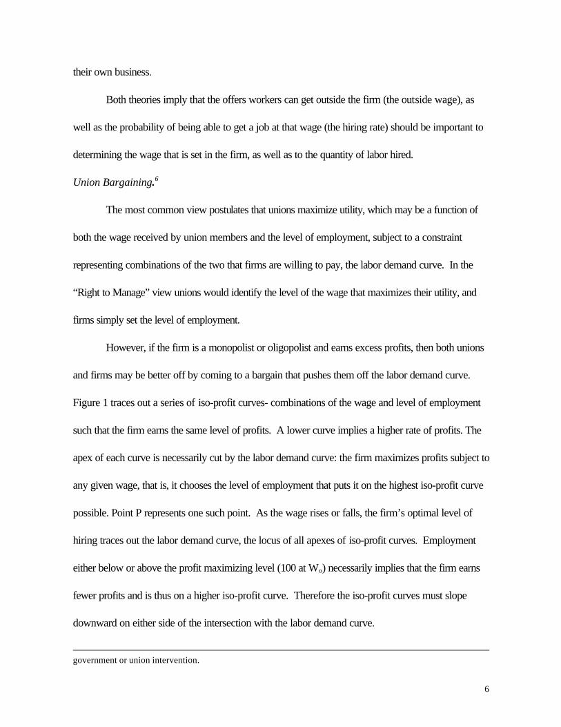
However, if the firm is a monopolist or oligopolist and earns excess profits, then both unions

and firms may be better off by coming to a bargain that pushes them off the labor demand curve.

Figure 1 traces out a series of iso-profit curves- combinations of the wage and level of employment

such that the firm earns the same level of profits. A lower curve implies a higher rate of profits. The

apex of each curve is necessarily cut by the labor demand curve: the firm maximizes profits subject to

any given wage, that is, it chooses the level of employment that puts it on the highest iso-profit curve

possible. Point P represents one such point. As the wage rises or falls, the firm’s optimal level of

hiring traces out the labor demand curve, the locus of all apexes of iso-profit curves. Employment

either below or above the profit maximizing level (100 at Wo) necessarily implies that the firm earns

fewer profits and is thus on a higher iso-profit curve. Therefore the iso-profit curves must slope

downward on either side of the intersection with the labor demand curve.

government or union intervention.

7

As point M in figure 2 shows, a better deal for both workers and firms can be negotiated

than that at “Right to Manage” equilibrium at point M. Here, the union’s utility curve is tangent to the

demand curve, but not to the iso-profit curve of the firms. Thus, the willingness of workers and firms

to trade off employment for wages is not equal, and the equilibrium is not efficient. Two alternate

and more efficient bargains where the two curves are tangent can easily be seen, both of them off the

labor demand curve. First, at point R, Unions reach a higher level of utility, UR compared to UM

while firms are earning the same level of profits. Alternately, at Q, unions are no worse off while firm

profits are higher. Which bargain, R, Q or perhaps Q’, where both are better off, are “efficient

bargains” and lie on the contract curve. The contract curve is the set of efficient bargains ranging

along the line PZ from P, where workers have no bargaining power and take the market wage W*

and the firm takes all profits, π*, to Z where πZ represents the level of profits below which the firm

would go out of business, and the union captures all of the monopoly rents. This iso-profit curve also

suggests that the maximum wage workers could ever gain would be Wz and then only if it cares very

little about employment.

These bargains along PZ, however, are clearly not efficient from a production point of view:

at any bargain except P, more workers are being hired than the firm would hire in the absence of a

union, E*. This “featherbedding” is a way of transferring firm profits to workers through the creation

of unnecessary positions, rather than wages. The final equilibrium clearly depends then on the goals

of the union as captured in the shape of its utility function, that jointly with the firm’s iso-profit

functions determines the contract curve, and the union’s relative bargaining strength, which

determines the position of the final bargain along the contract curve.

6 Graphs taken from and discussion based on Borjas (1996).

8

Both union objectives and bargaining power in Mexico may be different from those in

industrialized countries for a variety of reasons. First, like much of Latin America during the 1980’s

and early 90’s, job growth has been slow relative to population growth. Second, as is the case with

most of its neighbors, Mexico has no system of unemployment insurance and employment stability

may be more highly valued than wages. Third, since the post-revolution inception of the

Institutionalized Revolutionary Party (PRI) in 1929, the major unions have had a longstanding and

close relationship with the government. Particularly since 1987 with the inception of the Pacto- a

joint agreement of labor, business and the government to promote price stability- unions have closely

coordinated wage demands with pacto guidelines. These factors taken together may lead to an

emphasis on employment creation, relative to pushing up wages in the union utility function.

The next section details how empirically it is possible to determine whether the type of

bargaining occurring as well as if efficiency wage effects are important.

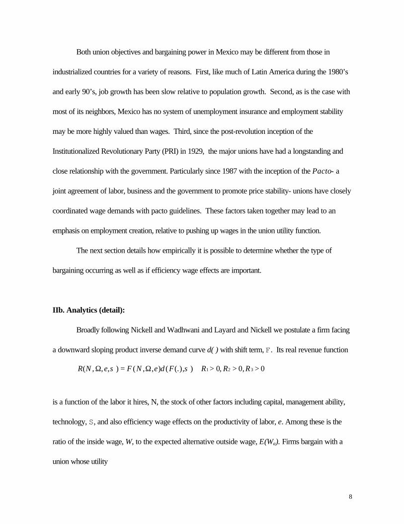
IIb. Analytics (detail):

Broadly following Nickell and Wadhwani and Layard and Nickell we postulate a firm facing

a downward sloping product inverse demand curve d( ) with shift term, F. Its real revenue function

R N e F N e d F R R R( , , , ) ( , , ) ( (.), ) , ,Ω Ωσ σ= > > >1 2 30 0 0

is a function of the labor it hires, N, the stock of other factors including capital, management ability,

technology, S, and also efficiency wage effects on the productivity of labor, e. Among these is the

ratio of the inside wage, W, to the expected alternative outside wage, E(Wa). Firms bargain with a

union whose utility

9

u U W E W N U U Ua= > < >( , ( ), ) , ,1 2 30 0 0

depends on the wage, the expected outside wage, and employment. In the “right to manage” model

the union bargains for a level of W, and lets the firm choose the level of employment. However, if the

union cares about employment as well, then its utility is maximized over both N and W and the

outcome is determined jointly in an “efficient bargain” with the firm. In this case, the firm moves off

the demand curve it would face in the RTM scenario and onto the contract curve.

The result of a standard Nash bargaining model yields a system of equations, both for

employment and the wage. The firm solution is a system of equations for labor demand and wages

of an (implicit) form such as

N N W E W Z ea N= ( , ( , , , )) 2 θ

W W E W Z e wa= ( ( , , , )) 2 θ

that reflect the compound effects of the two utility functions, as well as union bargaining power over

employment, 2N and the wage, 2w. Z2 contains variables that determine the position of the labor

demand relation, such as S,and F. The expected outside wage enters both through the union utility

function, and efficiency wage effects.

Several empirically testable predictions derive from the Nickell and Wadhwani and Layard

and Nickell framework which are testable with the Mexican data:

a. If unions bargain solely over the wage, then union power will be captured entirely in the

wages paid by the firm and free-standing proxies for union power should have no effect in labor

demand functions. Alternatively, if unions also bargain over the level of employment, the union proxy

should enter positively in the demand equation. In the extreme case that unions do not bargain over

the wage, but only employment, the union terms should be insignificant in the wage equation.

10

b. Since the workers’ alternative, the expected outside real wage adjusted for the probability

of getting a job, enters both in the firm’s calculation of the optimal efficiency wage as well as the

union utility function, its predicted sign and magnitude are ambiguous in cases where union power is

present.7 To avoid this problem, we will work with both unionized and non-unionized sectors to

search for efficiency wage effects.

c. The sign of the employment/wage elasticity depends on whether unions have more power

bargaining over employment or over wages.

d. As union power over employment determination 2 rises, the elements of Z2 (S, and F)

should lose influence in the labor demand equations.

We are particularly concerned with how these effects vary across a heterogeneous sample.

Most obviously, if unskilled workers are represented by unions more than the skilled, we may

observe different union and efficiency wage effects for each group. However the quantile analysis

detailed below also allows us to investigate whether these factors impinge differently across the

conditional distribution within these two samples.

III. Empirical Methodology

Conditional mean regression estimators, such as Ordinary Least Squares, are traditionally

used to estimate the relations such as those posited above. Minimizing the squared sum of errors

allows estimating the values of the parameters that predict the mean of the dependent variable,

conditional on a set of explanatory variables chosen. However, if the sample is not completely

homogeneous, such techniques may hide differential effects of the regressors across the distribution

7 Nickell and Wadhwani argue that the appearance in the demand function of outside wages indicates thepresence of efficiency wages unless unions both bargain over employment and more importantly, have a non-standard objective function, with the sign depending on the size of the standard employment-wage elasticity.

11

that may be a critical part of the story being told. Further, if there are large outliers, or the

distribution of the disturbances is non-normal, conditional mean estimators may be inefficient and

often biased.

These concerns can be reduced somewhat by estimating the conditional median regression

where half the errors lie above, and half below the fitted curve. Quantile analysis, introduced in

Koenker and Bassett (1978), extends this analysis to estimating curves where approximately J% of

the errors will be negative and (100-J)% of the errors will be positive.8 If the errors are i.i.d., slicing

the distribution at different quantile levels has little effect on parameter estimates and little information

is lost in a single measure of the conditional central tendency, such as the parameters generated by

OLS or median regression. However, figure 3 shows that asymmetries or heteroskedasticity in the

distribution of errors may lead to substantially different estimates of the impact of the variables under

study.

The problem of estimating an equation with endogenous explanatory variables under quantile

analysis was addressed successfully by Powell (1983). A two stage method, where a least square

regression is run on the first stage and median regression on the second as in 2SLS, was shown to

generate consistent estimates with asymptotically normal distributions under weaker assumptions than

least squares. This special case of a two-stage quantile regression (2SRQ) was generalized for any

quantile by Chen and Portnoy (1996).

In all the empirical work below, we present results of the quantile analysis at J=

50 (the conditional median regression) completely, J= 10 where 10% of the deviations lie below the

estimated regression, and J= 90 where 90% lie below. Appendix II presents the standard

12

conditional mean regressions, whether OLS or 2SLS for reference. In all cases they are very close

the median regression.

Correct Standard Errors for Two Stage Regression Quantiles

Standard errors estimates for regression quantiles have been studied in Buchinsky (1995) for

models with exogenous regressors. Based on a Monte Carlo study, the author recommends the use

of the design matrix bootstrap, as this method is valid under many forms of heterogeneity

(heteroscedasticity), with a small reduction in efficiency in iid samples, compared to other methods.

As in our model we cannot reject apriori heterogeneity (confirmed by LS based heteroscedasticity

tests), so we choose this method to estimate the covariance matrix of the regression parameter

vector.

The method amounts to sampling pairs (yi *,xi*) in a regression model yi = xi'β + ui to

generate a pseudo sample of the data and obtaining an estimate b* of β . The process is repeated B

times and the B estimates of β are used to construct the covariance matrix. The pseudo sample can

be of size n, the original sample size, as in this paper, and B should be large enough to guarantee a

small sample variability of the covariance matrix. We chose B=200, based on the literature. The use

of the design matrix bootstrap method for models with endogenous regressors can be argued for

using the results of Freeman and Peters (1994) on bootstrapping 2SLS models and the analogy

principle of estimation in Mansky (1988). In the present case, the covariance matrix for the labor

demand equations were obtained sampling the triplets (yi *,xi*, zi

* ), where zi is the vector of

instruments, or exogenous variables in the system and xi includes the endogenous explanatory

8 The technique has generally been applied to estimating returns to education, (Buchinsky 1994).

13

variables. Both first and second stage regressions are then run to obtain the estimates of the

parameter vector β for each of the B samples.

IV. Data:

We employ the Encuesta Nacional de Empleo, Salarios, Tecnologia y Capacitacion

(ENESTYC), the National Survey of Training, carried out by the Mexican Official Statistics Institute

(Instituto Nacional de Estadistica, Geografia e Informatica, INEGI) for the year 1992 which

contains detailed information on firms specific variables relating to employment, technology, capital

stock, etc. A 1995 Survey was also available that had the advantage of collecting data on share of

the work force unionized at the firm level. However, it lacked information on the human capital of

the work force and because the period it spanned contained the Tequila crisis in December 1994

and the beginning of the ensuing recession, we work primarily with what may be considered a more

“normal” period of relative prosperity.

14

Variables:

Core Variables:

Wages and Employment: Following Roberts and Skoufias (1997) and others the wage and labor

stock of skilled (Wsand Ns, respectively) and unskilled labor (Wuand Nu, respectively) are derived as

weighted averages of subcategories within each. The weights for constructing the labor variables

are the full wage (wage, social security and other non-wage benefits) per worker that capture the

relative “marginal product” of each subclass. This generates a compound measure of “efficient units”

of skilled or unskilled labor with the least productive subclass of labor as the numeraire in each.9 The

wage is then the total payments to the subclasses of labor divided by the labor measure, which, in

practice is simply the wage of the numeraire subclass. The average schooling of the unskilled is about

half of the skilled workers.

Value Added (Value Add.): the value of total 1991 output minus the expenses in materials and

energy in million Pesos.

Human Capital Variables:

Schooling (School and School2): Average years of schooling of the employed workers in each

skill level in the firm, where the years of schooling were obtained from 7 levels.

Experience(Experience and Experience2): Average tenure in the firm of workers within each sub-

class of labor.

9 This approach is arguably preferable to simply assuming that each subclass of workers has identical

productivity in the aggregation. In the skilled category are found directors (directivos) , Professionals(profesionista), Technical workers (tecnicos) , Administrative Employees (empleados administrativos) andSupervisors (supervisores). Among the Unskilled are professional workers (obreros profesionales) , specialists(especializados) and general workers (general).

15

As Dickens and Katz note, the most thorough test for efficiency wages are those that are

able to cross individual level human capital variables with plant level characteristics and control for

both. We are able only to control for the mean level of schooling in the plant and the mean tenure of

each category of workers within the plant. Though not a good measure of individual experience, the

latter is a good proxy for the accumulation of firm specific human capital and arguably better than the

potential experience variable (age-education) found in many articles (see, for example, Lam, and

Schoeni 1991).

Union and Efficiency Wage Variables:

Union Density (Union): The 1995 ENESTYC tabulates union density (ratio of firm employees

affiliated to a union) by individual firm while the 1992 only tabulates a dummy for the presence of

unionization in the firm. Under the assumption that union structure changes little over two years, we

assign a value of zero to the union density variable if the 1992 dummy is zero and the median sectoral

value from the 1995 survey if the 1992 dummy is unity.

Outside(alternative) wage (Wa): Log of the median sectoral wage, at the 4-digit industry level.

Hiring rate(Hiring): In the cross sectional context, the aggregate unemployment rate employed by

Nickell and Wadhwani is not useful10. We instead use the sectoral hiring rate (number of hires over

level of employment in the sector), as a measure of the probability of finding a job if you leave (with

your skills). This is more consistent with a labor turnover view of efficiency wages.

Quality Control (Qual. Con.): dummy for firms that have quality control of output.

10 The cross-section nature of the data and the impossibility of identification of the firm’s regional locationprecludes the use of an regional average wage, or typical informal sector earnings.

16

Productivity after Training (Training): dummy for firms that indicated increases in productivity

after implementing training programs.

Two size and eight sectoral dummies.

Shift parameters in Z2

Capacity Utilization (Cap. U.): average capacity utilization as reported by the firm in 1991.

Productivity: labor productivity measured as output per unit of labor. 11

Capital Labor Ratio (K/L): Log of the ratio of the reported value of capital stock over labor force.

Corporate: dummy for firms that belong to a corporation with multiple branches.

Foreign: dummy for firms with more than 50% foreign ownership.

Age (Age and Age2): age of the plant in years.

Export: dummy for firms with 10% or more of sales to other countries.

Automated: percentage of capital stock value of automated machinery.

Competiveness: dummy for firms that identify their product as “competitive” against imports.

Research and Development (R & D): dummy for firms with positive R&D expenses in 1991.

Technology Acquisition (Tech.): dummy for firms with positive expenses in technology acquisition

in 1991.

Observations with missing, incomplete, or zero entries for employment, output or capital

stock were dropped. We also only include privately owned firms and those with over 16

employees.12

11 To avoid a division bias in the productivity coefficient we use previous year productivity, as in Borjas (1980).Dropping this variable from the regressions does not change the results noticeably in general.12Micro firms (up to 15 employees), are extremely underrepresented in the sample and their heterogeneity cannotbe captured with the sample weights provided. INEGI has a specific survey of micro firms that is probably bettersuited to their analysis.

17

Table 1 presents the summary statistics of the variables employed. A few general

observations seem important. First, mean schooling of “unskilled” workers is half of those identified

as “skilled,” and the mean unskilled experience is slightly smaller than that of skilled workers,

possibly due to higher turnover. Second, only 17,8% of the firms do not have their workers

associated with a central sindical (union) so there are roughly five times the number of observations

in the union sample than the non-union sample. This can make comparisons of the significance of

effects occasionally ambiguous. Within the union sample, the mean unionization rate is 55%. Third,

Mann-Whitney tests show that the unconditional distributions of most variables differ between the

unionized and unionized samples.13 This suggests that the two samples differ in fundamental ways

and perhaps should not be combined during the analysis.

Va. Empirical Results: Wage Equations

By contrast to the standard competitive model where firms take wages as given, the

framework above makes it clear that wages and employment are determined jointly and hence

constitute a system of equations to be estimated. However, standard wage equations with

employment omitted can be thought of as a reduced form and can be estimated using one step

estimators such as least squares or median regression. Broadly following Dickens and Katz(1987)

and Nickell and Wadhwani we estimate the log linear approximation

w W us u w e u h x wa, = + + + + +a e h xγ γ γ γ γ ε

13 Standard equality of mean and variances tests were not employed as the unconditional distributions are clearlynon-normal.

18

where wa is a vector of proxies for the expected alternative wage, e a vector of other possible

efficiency wage related variables, u, the union power measure, h a vector of human capital variables,

x the vector of firm related characteristics, including those in Z2.

1. General Results

Tables 2.1-2.2 present the quantile results for the non-union and union groups respectively.

In all cases, the regressions are significant at the 0 % level. The pseudo-R2 of the median regression

specifications explains 29% of the variance for skilled unionized, 11.5% for those unskilled, and for

the non-unionized sample 37.8% and 15.6% respectively.14

Several of the shift variables enter with expected signs and magnitudes although others are

more ambiguous. The impact of productivity on wages in both samples is of comparable size as in

the literature (Wadhwani and Wall 1991) although it enters insignificantly for skilled non-union

workers and of significantly larger coefficient for non-union unskilled. Among union firms,

productivity is insignificant at the 10th quantile suggesting that for this part of the distribution, union

power may possibly delink productivity from wages. Exporters pay significantly more to skilled

union workers in the 10th quantile and unskilled union in the 50th and 90th quantile, although the

indicator of product competitiveness is never significant in any regression suggesting that greater

openness does not obviously depress wages. Foreign firms pay skilled workers less across all

quantiles and unskilled workers significantly more in the 90th quantile. R& D enters positively at the

median only for non-unionized skilled workers, technology purchases enter strongly and of the

predicted sign only in the unionized sector (with the exception of the 90th quantile), indicating that

14 Pseudo R2 defined as squared correlation between original and fitted observations. The standard versionbased on the decomposition of total variation between fitted and residual values is not correct for quantileanalysis.

19

union firms use more productive technology. K/L enters positively for non-union unskilled workers at

the 90th quantile. Automated never enters significantly.

These results are similar to those from the OLS regressions presented in Appendix 2.

Appendix figures A1.1-A1.4 show that the predicted relation between wages and employment is

very similar in both cases.

2. Union Effects

The union and non-union samples were run separately for two reasons. First, we are

interested in isolating efficiency wage effects that, as in the case of the outside wage, are sometimes

hard to disentangle from union effects. Second, there may be serious problems of selection bias in

measuring union premia. In preliminary regressions, we find that a union dummy in the combined

sample suggests that firms with unions pay 15.2% more to skilled workers and 9.25% more than

non-union firms and the continuous union density variable enters positively and significantly as well.

However, it is very difficult to know whether unions cause wage differentials, or whether unions are

more likely to be found in certain types of firms who also pay higher wages. As an example,

schooling enters significantly across all sub-samples, but experience enters only in the union sample.

The average union worker with five years of experience would make roughly 12% more than his

non-union counterpart and the unskilled perhaps 8%. Constraining the experience coefficient to be

equal across sub-samples could give rise to differentials of the magnitudes of the union dummies. If

the differing coefficients represent rigidly enforced seniority base promotions or wage hikes, then the

differential might legitimately capture union power (see Borjas 1996). However, if firms use

production techniques that require more on-the-job training and also make them more prone to

20

unionization, then the differentials capture legitimate differences in human capital rather than union

power.

As mentioned earlier, Mann-Whitney tests show that the unconditional distributions of most

variables differ between the unionized and non-unionized sample, and Chow tests for the equality of

the coefficients between union and non-union firms strongly reject at the 1% level, consistent with the

view that union and non-union firms may be fundamentally different. As a strategy that partially

alleviates the selection bias problem, we test for the impact of union power within the sample of

firms with unions.

In a very surprising result, the free-standing union term virtually never enters significantly as

would be predicted by traditional right to manage models.15 The labor demand regressions in the next

section will cast doubt on the obvious interpretation that unions have no power. But the quantile

regressions also reveal a story hidden to standard techniques. For the upper quantiles, there is no

impact on unskilled wages. However, for the 10th quantile a strong and positive coefficient emerges

on the union density term while the human capital variables that are important for the other quantiles

largely disappear. An interpretation is that workers who earn little given measured human capital,

are helped by unions. If for example, a worker’s unobserved characteristics, such as reliability and

diligence, dictate a low wage relative to those who, on paper, appear similar, unions will push them

toward the average for their class. To the degree that this measures distortion in the wage

distribution, it appears to be confined to the 10th quantile. Overall, union density does not

appear to have a major impact on unskilled wages.

15 This contrasts with the findings of Panagides, A. and H.A. Patrinos (1994). However, their finding of unionimpact on wages probably arises from the fact that they could not control for firm size or other charateristics.

21

A striking result is the strong negative impact of union density on skilled wages, precisely the

opposite effect found in the combined regression. This may be due to more successful unskilled

worker bargaining over firm rents (distributed in forms other than wages), or it may be related to a

desire to reduce the wedge between skilled and unskilled remuneration for equity reasons.

3. Efficiency Wage Effects

Outside wages enter for all union worker types and most quantiles, skilled non-unionized

workers at the median and the 10th quantile for unskilled non-union. The significance of the outside

wage in both the union and non-union samples, although less strikingly, suggests that its influence is

more than simply a reference for union bargaining. Further, the magnitude of the impact for unskilled

workers at the 10th quantile is double that for the union sector and almost double for skilled workers

at the 50th. For both samples, at the 90th quantile, outside wage effects drop dramatically in

significance and magnitude for skilled workers. A possible interpretation is that workers paid well

given their human capital are likely to receive a larger share of total remuneration and the efficiency

wage premium in unobservable non-wage benefits.

Somewhat counterintuitively, the hiring rate enters with unexpected sign although

insignificantly in all but the unionized skilled worker sample at the 50th and 90th quantiles. Whether

training had been undertaken that was perceived as productivity enhancing has the predicted sign for

non-union skilled workers and high wage unskilled non-union workers. Inter-industry wage

differentials (Krueger and Summers 1988) as captured by sectoral dummies are not very strong in

most sectors after controlling for human capital variables in firms, contrary to much of the literature.

On the other hand, firm size effects, are strongly present as in Schaffner (1998). For both union and

22

non-union firms, apparently similar skilled workers in small firms of between 16 and 100 workers

make roughly 50% less in wages and benefits than they would in a firm of over 250. In the event

that this is in fact, due to efficiency wage considerations arising, perhaps from difficulties of

monitoring, the implicit segmentation emerging endogenously among formal enterprises is very large.

Vb. Empirical Results: Labor Demand

The data allow the estimation of system of skilled and unskilled labor demand functions and

hence the examination of unions’ impact on the substitutability of factors and the allocative efficiency

of firms. We estimate log-linear approximations to both equations.

n q us u w q w u x na, = + + + + +w w xaβ β β β β ε

ns,u is the log of labor demand for skilled (NS) or unskilled labor (NU), w=log(WS, WU) the vector

of log own and cross wages16 q, log firm output, wa the vector of proxies for own and cross-

expected alternative outside wages (log outside wages and the sectoral hiring rates), u the measure

of union bargaining power, x the vector of other firm characteristics.

Ideally, the labor demand equation would be estimated using instruments for wages due to

possible measurement error, random productivity shocks, and the fact that unions may bargain over

both wages and employment simultaneously.17 However, good instruments prove difficult to find. We

are not working with panel data and, as the previous section suggests, the most complete model for

the unskilled wage explains relatively little of the variance. The results, as Roberts and Skoufias found

16 As in Roberts and Skoufias we do not have a measure for the capital services price. We use the corporationdummy as well as the level of automated machinery and firm size dummies to differentiate the firms on theiropportunity costs of capital services.17 Hours composition bias (Hamermesh) does not seem to be a problem in our data as the majority of firms did notchange the number of weekly and daily shifts across a six month period in 94-95, during the tequila crisis.

23

for Colombia, were counter-intuitive.18 Output should be considered endogenous also, due to

measurement error (current output different from the output used in the decision making of the firm)

and the presence of unobserved firm specific shocks that affect output and employment. This is

confirmed by Durbin-Hausman-Wu (Davidson and MacKinnon, 1993) tests. With more success

we instrument using the capital stock (and its square), capacity utilization levels and other firm

specific technology variables. Chow tests for the equality of coefficients between union and non-

union firms for skilled and unskilled workers respectively reject at conventional significance levels.

Again, it is clearly not appropriate to combine the samples and we report separate regressions for

each group.

1. General Results

Tables 3.1 and 3.2 present the results from a static labor demand equation for the non-

unionized and unionized sectors respectively. The regressions are broadly consistent with standard

factor demand theory (see, for example, Chambers 1988 and Hamermesh) and other empirical

studies. Own-wage elasticities strongly suggest a downward labor demand relation in both sectors.

Output elasticities are statistically similar in both samples, as expected by theory under the hypothesis

of a homothetic technology. Their small magnitude suggests that firms are operating in the downward

sloping part of the long run average cost curve, as in a monopolistic competition model. Cross-wage

18 In both union and non-union firms using OLS, we have an upward sloping demand curve for skilled labor. Inthe former a flat demand curve for unskilled workers appeared with “wrong” signed outside wage effects for both(yet consistent with the wrong insignificant inside wages coefficients). The large union effect was maintained forunskilled. Hiring rates never entered significantly. The (naive) R2 for unskilled fell from .68 to .15. We attributethe results to the unavailability of good instruments (hinted by the non-rejection of Durbin-Hausman-Wu testsfor unskilled workers) and present only the results with non-instrumented wages and lagged output.

24

effects are zero for all median regressions.19 Morishima elasticities of substitution between types of

labor are in the 60-35% range, and if we assume that total labor costs are half that of the capital

services (10% of the capital stock) the capital-unskilled elasticity of substitution labor seems to be

around 0.5 and nearly twice that of the capital-skilled labor, as in the references in chapter 3 of

Hamermesh.20

Estimating the relation across quantiles adds additional information. Perhaps unsurprisingly,

firms who have a large workforce after adjusting for the variables in the regression show higher

output elasticities and hence smaller scale economies across all sub-samples operating closer to the

long run minimum of the average cost curve. This is most striking for the case of non-union skilled

workers where the 10th quantile has an output elasticity of .22 which rises to .58 in the 90th quantile.

Figures A2.1-2.4 in the appendix illustrate what these differences imply for the employment

trajectory for each quantile level. The 90th quantile employ vastly more additional workers for an

additional unit of output than the firm at the conditional median and this appears particularly to be the

case for unskilled labor where the distribution appears far less symmetric than is the case for skilled

workers.

Less obviously, these firms with lower economies of scale also show higher elasticities of

substitution. For skilled workers, own elasticities quadruple and double for non-union and union

firms respectively across the quantile range and also substantially increase for unskilled workers

19 Both labor types seem to be substitutes for capital, with the cross price unskilled labor-capital elasticity largerin absolute value than the skilled-capital elasticity. Roberts and Skoufias results suggest also monopolisticcompetition and skilled and unskilled workers have negative cross price elasticities, i.e., they are complements.20 Morishima elasticities of substitution measure how much the ratio of factor used, rather than simply theamount of one factor, changes with respect to one of the factor prices. In unionized firms, the ratio of labor typesmean wage costs is close to one and about 0.85 for non-union. We use the fact that factor demands arehomogeneous of degree zero in prices to obtain the capital elasticities.

25

although less dramatically. This, increase across quantiles can be seen in appendix figures A2.1-2.4.

No clear pattern emerges for cross elasticities across quantiles.

Several of the proposed demand shift variables enter significantly and of expected sign.

Capacity utilization, as a measure of factor usage is positive in all regressions although clearly

significantly so only for unskilled at the 50th quantile for non-unionized and for the 10th in the both

the unionized groups and 50th for the unskilled. The virtual absence of any significant effect among

skilled workers with the exception of a counterintuitive negative effect for the 10th quantile in the

union sample suggests skilled labor hoarding. Exporting firms hire roughly 15-20% more unskilled

and perhaps 0- to 4% more skilled workers (never significant) as would be expected given that 82%

of these firms engage in some maquila work that is particularly labor intensive.

Foreign firms tend to hire more workers, relative to national although only statistically

significantly so across all quantiles of the union skilled sample. Older union firms have more skilled

workers although not significantly more unskilled. Whether the firm is part of a large corporation

enters positively for all groups for at least the lower quantile, and not for the upper quantile.

2. Union Effects

Although the previous section suggested that there were no union effects on wages, union

density has a strong positive effect on the level of unskilled employment across all quantiles. This

suggests a unique example of efficient bargaining where unions accept the market wage, but cause

firms to move off the demand curve to hire more labor. The regressions suggest that across all

26

quantiles, for each 1% of the work force that is unionized, unskilled employment appears to increase

by roughly 2.5%. Despite this, we find little reduction in the magnitude of the shift terms, such as

capacity utilization, foreign ownership, and membership in a larger corporation as the analytical

overview suggests should happen, and the clear downward sloping demand relation is preserved.

This suggests that the position on the contract curve may not be “too far” from the demand curve.

However, estimates of the impact of unions on productivity (not shown) confirm the intuition that

there is a significant adverse effect arising from the additional labor hired.

Somewhat counterintutively, the regressions for skilled workers find a negative union effect,

although one that is only remotely significant is the top quantile where a 1 point rise in the percentage

unionized leads to a roughly equal equivalent fall in the number of skilled laborers. This might suggest

that, among firms with conditionally high levels of employment, unions represent primarily unskilled

workers and “crowd out” those more skilled. Alternatively, perhaps when unions seek to organize,

they pick firms with conditionally large labor forces, but within this group choose those with relatively

more unskilled workers.

As might be expected, union firms have statistically significant, although not substantially

smaller own wage elasticities that might suggest slightly less flexibility in the allocation of unskilled

workers. However, the pattern is reversed for skilled workers and the large employment firms

appear to be driving this result. For conditionally small firms, the union sample for unskilled labor has

a higher point estimate than that of the non-union sector and at the median, there is no noticeable

difference.

The presence of unions has little impact on output elasticities. A firm with 10% higher output

is likely to hire roughly 4% more skilled. This is not necessarily surprising since a greater hiring rate

27

of workers by unionized firms occurs on top of a larger base, leaving the elasticity virtually

unchanged.

In sum, unions appear to concentrate their efforts on featherbedding, but it is not obvious that

they reduce flexibility in allocating factors. It also appears that unions have the effect of reducing the

dispersion of elasticities across quantiles.

3. Efficiency wage effects.

There is evidence of efficiency wage effects in the demand functions as well. As Nickell and

Wadhwani show, the expected outside wages and hiring probabilities can enter in the demand

function in the unionized sector even when there are no efficiency wage effects because unions may

use them for reference. However, the outside wage, and the probability of hiring enters strongly for

unskilled non-union workers. In the union sector, the hiring rates are significant at the median for the

skilled but outside wages are, in general, either counter-intuitive or insignificant.

Focusing on the non-union sector, the quantile regressions suggest that the outside wage

effects are fairly consistent across quantiles-unimportant for skilled workers and of similar

magnitudes and significant for unskilled. No clear story emerges from the coefficients on hiring rates.

VI. Conclusion

Two provocative findings emerge from this paper. First, Mexican unions do not seem to

show “right to manage” behavior and their impact on wages appears relegated to putting a floor

under the conditionally least well paid workers (10th quantile). Nonetheless, they do greatly increase

the quantity of unskilled workers hired and appear to “crowd out” skilled workers in what appears

to be an extreme form of Efficient Bargaining. The impact on productivity is, by definition negative,

28

but the flip side may be that unions are forcing firms to use “appropriate” technology that uses

relatively less capital and more unskilled workers. As Layard and Nickell have noted, the general

equilibrium effects on the overall level of labor employed in the economy are clear: if unions bargain

over employment as well as wages, as seems to be the case here, employment in the union sector

should be higher, under a smaller than unity elasticity of substitution, as also seems to be the case

here. It is therefore possible that far from reducing the level of employment by rationing workers into

the informal sector, Mexican unions may be preserving low skilled jobs, at the cost of smaller

wages.21

The second important finding is that there appears to be strong evidence of efficiency wage

effects. A tentative conclusion would be therefore, that whatever segmentation is observed, defined

as equivalent workers earning different wages, is more likely to be emerging from the efficiency wage

effects than from union effects. This would suggest that, even in the absence of minimum wages or

union power, substantial segmentation will remain in Mexico as well as other LDCs.

References:

Abuhadba, M and P. Romaguera (1993), “Inter-Industrial Wage Differentials:Evidence from LatinAmerican Countries” Journal of Development Studies 30(1), 190-205.

Bell, L (1997) “The Impact of Minimum Wages in Mexico and Colombia” Journal of laborEconomics, 15(3), Part 2 S102-35.

Blanchflower, D.C., N. Millward and A. J. Oswald (1991), “Unionism and Employment Behaviour,”The Economic Journal, 101 815-834.

Borjas, G. (1980) “The Relationship Between Wages and Weekly Hours of Work: the Role ofDivision Bias.” The Journal of Human Resources 15(3) 409-423. 21 For an analysis of the differential impact on labor markets of economic reform under different types of unionbehavior, including the “featherbedding” found here, see Devarajan, Ghanem and Thierfelder (1997).

29

Borjas, G. (1996), Labor Economics, New York:McGraw-Hill.

Brooks, D. and J. Cason (1998), “Mexican Unions: Will Turmoil Lead to Independence?” WorkingUSA, March-April.

Buchinsky, M. (1994) “Changes in the US Wage Structure 1963-87: An application of quantileregression”. Econometrica, 62(3), 405-458.

Buchinsky, M. (1995). Estimating the asymptotic covariance matrix for quantile regression models: aMonte Carlo study. Journal of Econometrics 68, 303-38.

Chambers, R.G.(1988) Applied Production Analysis, A Dual Approach, Cambridge: CambridgeUniversity Press.

Chen, L.-A. and Portnoy, S. (1996). Two-stage regression quantiles and two stage trimmed leastsquares estimators for structural equation models. Communications in Statistics- Theory andMethods 25(5), 1005-1032.

Collier, R. and D. Collier (1991), Shaping the Political Arena, Critical Junctures, the Labormovement, and Regime Dynamics in Latin America, Princeton University Press, Princeton.

Davidson, R. and MacKinnon, J.(1993). Estimation and Inference in Econometrics. NewYork:Oxford University Press.

Devarajan, S, H. Ghanem and K. Thierfelder (1997), “Economic Reform and Labor Unions: AGeneral-Equilibriium Analysis Applied to Bangladesh and Indonesia,” World Bank EconomicReview 11(1):145-170.

Dickens, W.T and L.F. Katz (1987) “Inter-industry Wage Differences and Industry Characteristics”in K. Lang and J.S. Leonard eds., Unemployment and the Structure of Labor Markets, NewYork: Blackwell.

Esfahani, H. and D. Salehi-Isfahani (1989) “Effort Observability and Worker Productivity: Towardsan Explanation of Economic Dualism,” Economic Journal, 99 818-836.

Freedman, D. and Peters, S. (1984) Bootstrapping an Econometric Model: some empirical results.Journal of the American Statistical Association 79, 97-106.

Funkhouser, E. (1998) “The Importance of Firm Wage Differentials in Explaining Hourly EarningsVariation in the Large Scale Sector of Guatemala” Journal of Development Economics 55(1),115-131.

30

Hamermesh, D.(1993). Labor Demand. Princeton: Princeton University Press.

Harris, J.R. and M.P. Todaro (1970) “Migration, Unemployment and Development: A Two SectorAnalysis,” American Economic Review, 60:1, 126-142.

Hendricks and Kahn (1991), “Efficiency Wages, Monopoly Unions and Efficient Bargaining,”Economic Journal, 101(408), 1149-62.

Koenker, R. and G. Bassett (1982), “Regression Quantiles”, Econometrica, 46, 33-50.

Krueger, A.B and L. H. Summers (1988), “Efficiency Wages and the Inter-Industry WageStructure”, Econometrica 56(2), 259-293.

Lam, D. and Schoeni, R. Effects of family background on earnings and returns to schooling: evidencefrom Brazil. Journal of Political Economy 101, 710-740.

Layard, R. and Nickell, S.(1990). Is Unemployment Lower If Unions Bargain Over Employment?Quarterly Journal of Economics 105(2), 773-787.

Lewis G.H. (1986) “Union Relative Wage Effects” in: O. Ashenfelter and R. Layard eds.,Handbook of Labor Economics, v.2, Amsterdan:North-Holland.

Manski, C. (1988) Analog Estimation Methods in Econometrics New York:Chapman and Hall.

Marquez, G. (1990) “Wage Differentials and Labor Market Equilibrium in Venezuela,” UnpublishedPh.D. Dissertation, Boston University.

Marquez, C. and J. Ros(1990), “Segmentacion del Mercado de Trabajo y Desarrollo Economic enMexico”, El Trimestre Economico, Fondo de Cultura Economica, Mexico, 17:2

Nickell, S. and Wadhwani,W. (1990) “Employment Determination in British Industry: InvestigationsUsing Micro-Data,” Review of Economic Studies, 58(5), 955-969.

Oswald, A. J.(1991) Efficient Contracts Are on the Labour Demand Curve, Labour Economics,1(1), 85-113.

Panagides, A. and H.A. Patrinos (1994), “Union-Non-Union Wage Differentials in the DevelopingWorld” World Bank Policy research working Paper 1269.

Phelps, E.(1994) Structural Slumps: The Modern Theory of Unemployment, Interest, andAssets, Cambridge, MA: Harvard University Press.

Powell, J.L. (1983). The asymptotic normality of tow-stage least absolute deviations estimators.

31

Econometrica, 51, 1569-1576.

Roberts, M. and Skoufias, E.(1997). The Long Run Demand for Skilled and Unskilled Labor inColombian Manufacturing Plants. Review of Economics and Statistics 79(1), 330-334

Schaffner, J.A.(1998) “Premiums to Employment in Larger Establishments: evidence from Peru.Journal of Development Economics 55(1), 81-113.

Stiglitz, J.E.(1974) “Alternative Theories of Wage Determination and Unemployment in LDC’s: TheLabor Turnover Model, “ Quarterly Journal of Economics, 88(1), 194-227.

Wadhwani, S. B and M. Wall (1991), “A Direct Test of the Efficiency Wage Model Using UKMicro-Data,” Oxford Economic Papers, 43(2), 529-548.

Weiss, A. (1990). Efficiency Wages. Princeton: Princeton University Press.

32

Table 1 – SUMMARY STATISTICSNon-Union (n=731) Union (n=3,421)

Variable Mean Std.Dev. Min Median Max Mean Std.Dev. Min. Median MaxForeign 0.331 0.471 0.000 0.000 1.000 0.198 0.398 0.000 0.000 1.000Age 17.036 13.414 1.000 12.000 99.000 25.188 16.123 1.000 23.000 99.000Cap. U.* 75.104 19.339 5.000 80.000 100.000 74.479 18.102 1.000 80.000 100.000Exporter 0.438 0.496 0.000 0.000 1.000 0.241 0.427 0.000 0.000 1.000R & D 0.334 0.472 0.000 0.000 1.000 0.383 0.486 0.000 0.000 1.000Tech. 0.454 0.498 0.000 0.000 1.000 0.508 0.500 0.000 1.000 1.000Qual. Cont. 0.988 0.110 0.000 1.000 1.000 0.997 0.057 0.000 1.000 1.000Corporate* 0.252 0.434 0.000 0.000 1.000 0.257 0.437 0.000 0.000 1.000Union 0.680 0.074 0.477 0.703 0.854Ws 9.422 0.907 5.991 9.573 11.352 9.827 0.726 5.849 9.909 12.110Ns 1.587 1.011 0.000 1.444 6.685 1.973 0.956 0.000 1.890 6.472Wu 7.765 0.754 5.758 7.744 10.134 7.983 0.688 5.659 8.032 11.160Nu 3.449 1.342 0.000 3.466 8.964 3.842 1.135 0.000 3.809 8.606School- S* 11.962 2.120 3.000 12.150 18.500 12.150 1.708 4.909 12.233 17.843School –U 6.603 1.497 3.000 6.450 12.000 6.873 1.321 3.000 6.783 12.000Experience-S 5.495 3.385 0.294 4.483 25.640 6.631 4.000 0.065 5.663 32.927Experience-U 4.124 3.787 0.000 3.000 38.000 5.817 4.864 0.000 4.118 40.000Value Add.* 8.274 1.717 1.792 8.343 14.878 9.250 1.597 1.386 9.263 15.072Productivity- S 6.686 1.204 1.068 6.750 12.472 7.277 1.116 0.372 7.328 13.008Productivity-U 4.824 1.441 -0.508 4.797 10.811 5.408 1.241 -2.635 5.435 10.659Wa-U 7.837 0.210 6.742 7.899 8.189 7.847 0.193 6.742 7.825 8.189Wa-U 9.563 0.325 7.784 9.578 10.182 9.641 0.293 7.784 9.708 10.182Automated* 12.726 23.325 0.000 0.000 100.000 11.837 22.601 0.000 0.000 100.000Log(K) 7.716 1.980 2.303 7.690 14.526 9.021 2.000 1.609 9.131 15.735Log K/Nu 3.186 1.838 -2.896 3.232 9.573 4.013 1.666 -3.626 4.191 10.125Log K/Ns 4.342 1.635 -0.984 4.397 10.978 5.040 1.514 -1.686 5.194 10.877Hireing-U 7.512 3.972 0.322 6.628 15.240 6.857 3.468 0.322 6.052 15.240Hireing-S. 1.079 0.512 0.000 1.043 2.641 1.199 0.602 0.000 1.091 2.641Training 0.211 0.408 0.000 0.000 1.000 0.236 0.425 0.000 0.000 1.000Competitive 0.512 0.500 0.000 1.000 1.000 0.631 0.483 0.000 1.000 1.000Source: author’s calculation from ENESTYC ‘92. Large, medium and small firms only (from 16 employees on). * - Mann-Whitney test does not reject equality of distributions between union and non-union samples. Seevariable definitions in text.

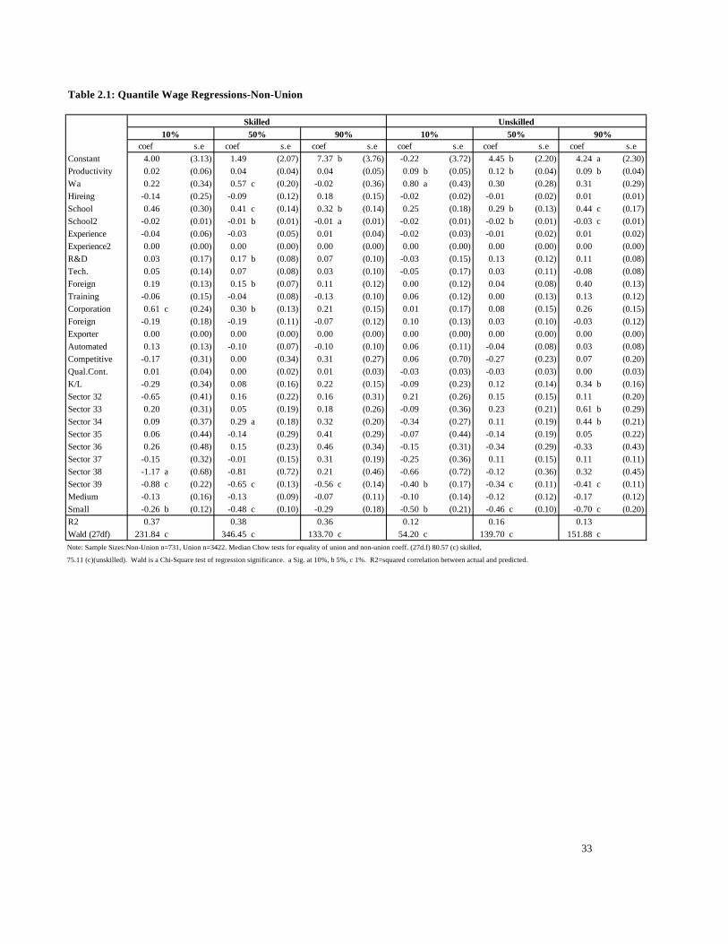
Table 2.1: Quantile Wage Regressions-Non-Union

coef s.e coef s.e coef s.e coef s.e coef s.e coef s.eConstant 4.00 (3.13) 1.49 (2.07) 7.37 b (3.76) -0.22 (3.72) 4.45 b (2.20) 4.24 a (2.30)Productivity 0.02 (0.06) 0.04 (0.04) 0.04 (0.05) 0.09 b (0.05) 0.12 b (0.04) 0.09 b (0.04)Wa 0.22 (0.34) 0.57 c (0.20) -0.02 (0.36) 0.80 a (0.43) 0.30 (0.28) 0.31 (0.29)Hireing -0.14 (0.25) -0.09 (0.12) 0.18 (0.15) -0.02 (0.02) -0.01 (0.02) 0.01 (0.01)School 0.46 (0.30) 0.41 c (0.14) 0.32 b (0.14) 0.25 (0.18) 0.29 b (0.13) 0.44 c (0.17)School2 -0.02 (0.01) -0.01 b (0.01) -0.01 a (0.01) -0.02 (0.01) -0.02 b (0.01) -0.03 c (0.01)Experience -0.04 (0.06) -0.03 (0.05) 0.01 (0.04) -0.02 (0.03) -0.01 (0.02) 0.01 (0.02)Experience2 0.00 (0.00) 0.00 (0.00) 0.00 (0.00) 0.00 (0.00) 0.00 (0.00) 0.00 (0.00)R&D 0.03 (0.17) 0.17 b (0.08) 0.07 (0.10) -0.03 (0.15) 0.13 (0.12) 0.11 (0.08)Tech. 0.05 (0.14) 0.07 (0.08) 0.03 (0.10) -0.05 (0.17) 0.03 (0.11) -0.08 (0.08)Foreign 0.19 (0.13) 0.15 b (0.07) 0.11 (0.12) 0.00 (0.12) 0.04 (0.08) 0.40 (0.13)Training -0.06 (0.15) -0.04 (0.08) -0.13 (0.10) 0.06 (0.12) 0.00 (0.13) 0.13 (0.12)Corporation 0.61 c (0.24) 0.30 b (0.13) 0.21 (0.15) 0.01 (0.17) 0.08 (0.15) 0.26 (0.15)Foreign -0.19 (0.18) -0.19 (0.11) -0.07 (0.12) 0.10 (0.13) 0.03 (0.10) -0.03 (0.12)Exporter 0.00 (0.00) 0.00 (0.00) 0.00 (0.00) 0.00 (0.00) 0.00 (0.00) 0.00 (0.00)Automated 0.13 (0.13) -0.10 (0.07) -0.10 (0.10) 0.06 (0.11) -0.04 (0.08) 0.03 (0.08)Competitive -0.17 (0.31) 0.00 (0.34) 0.31 (0.27) 0.06 (0.70) -0.27 (0.23) 0.07 (0.20)Qual.Cont. 0.01 (0.04) 0.00 (0.02) 0.01 (0.03) -0.03 (0.03) -0.03 (0.03) 0.00 (0.03)K/L -0.29 (0.34) 0.08 (0.16) 0.22 (0.15) -0.09 (0.23) 0.12 (0.14) 0.34 b (0.16)Sector 32 -0.65 (0.41) 0.16 (0.22) 0.16 (0.31) 0.21 (0.26) 0.15 (0.15) 0.11 (0.20)Sector 33 0.20 (0.31) 0.05 (0.19) 0.18 (0.26) -0.09 (0.36) 0.23 (0.21) 0.61 b (0.29)Sector 34 0.09 (0.37) 0.29 a (0.18) 0.32 (0.20) -0.34 (0.27) 0.11 (0.19) 0.44 b (0.21)Sector 35 0.06 (0.44) -0.14 (0.29) 0.41 (0.29) -0.07 (0.44) -0.14 (0.19) 0.05 (0.22)Sector 36 0.26 (0.48) 0.15 (0.23) 0.46 (0.34) -0.15 (0.31) -0.34 (0.29) -0.33 (0.43)Sector 37 -0.15 (0.32) -0.01 (0.15) 0.31 (0.19) -0.25 (0.36) 0.11 (0.15) 0.11 (0.11)Sector 38 -1.17 a (0.68) -0.81 (0.72) 0.21 (0.46) -0.66 (0.72) -0.12 (0.36) 0.32 (0.45)Sector 39 -0.88 c (0.22) -0.65 c (0.13) -0.56 c (0.14) -0.40 b (0.17) -0.34 c (0.11) -0.41 c (0.11)Medium -0.13 (0.16) -0.13 (0.09) -0.07 (0.11) -0.10 (0.14) -0.12 (0.12) -0.17 (0.12)Small -0.26 b (0.12) -0.48 c (0.10) -0.29 (0.18) -0.50 b (0.21) -0.46 c (0.10) -0.70 c (0.20)R2 0.37 0.38 0.36 0.12 0.16 0.13Wald (27df) 231.84 c 346.45 c 133.70 c 54.20 c 139.70 c 151.88 cNote: Sample Sizes:Non-Union n=731, Union n=3422. Median Chow tests for equality of union and non-union coeff. (27d.f) 80.57 (c) skilled,

75.11 (c)(unskilled). Wald is a Chi-Square test of regression significance. a Sig. at 10%, b 5%, c 1%. R2=squared correlation between actual and predicted.

33

Skilled Unskilled10% 50% 90% 10% 50% 90%

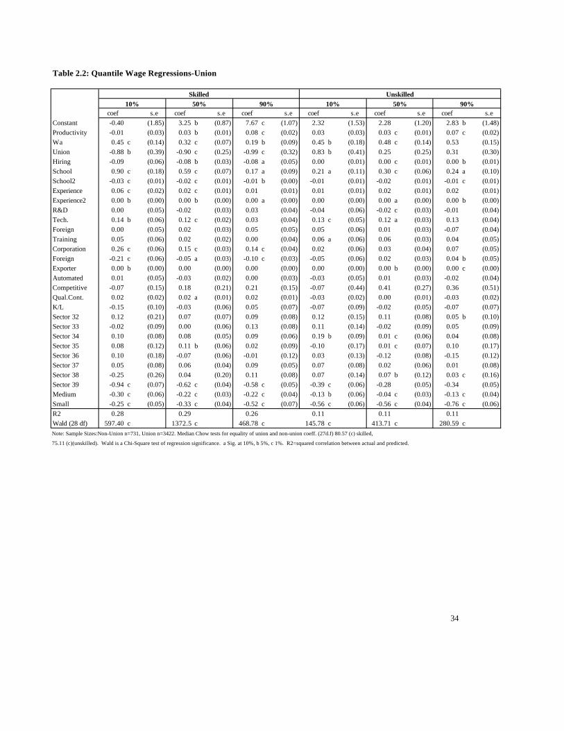
Table 2.2: Quantile Wage Regressions-Union

coef s.e coef s.e coef s.e coef s.e coef s.e coef s.eConstant -0.40 (1.85) 3.25 b (0.87) 7.67 c (1.07) 2.32 (1.53) 2.28 (1.20) 2.83 b (1.48)Productivity -0.01 (0.03) 0.03 b (0.01) 0.08 c (0.02) 0.03 (0.03) 0.03 c (0.01) 0.07 c (0.02)Wa 0.45 c (0.14) 0.32 c (0.07) 0.19 b (0.09) 0.45 b (0.18) 0.48 c (0.14) 0.53 (0.15)Union -0.88 b (0.39) -0.90 c (0.25) -0.99 c (0.32) 0.83 b (0.41) 0.25 (0.25) 0.31 (0.30)Hiring -0.09 (0.06) -0.08 b (0.03) -0.08 a (0.05) 0.00 (0.01) 0.00 c (0.01) 0.00 b (0.01)School 0.90 c (0.18) 0.59 c (0.07) 0.17 a (0.09) 0.21 a (0.11) 0.30 c (0.06) 0.24 a (0.10)School2 -0.03 c (0.01) -0.02 c (0.01) -0.01 b (0.00) -0.01 (0.01) -0.02 (0.01) -0.01 c (0.01)Experience 0.06 c (0.02) 0.02 c (0.01) 0.01 (0.01) 0.01 (0.01) 0.02 (0.01) 0.02 (0.01)Experience2 0.00 b (0.00) 0.00 b (0.00) 0.00 a (0.00) 0.00 (0.00) 0.00 a (0.00) 0.00 b (0.00)R&D 0.00 (0.05) -0.02 (0.03) 0.03 (0.04) -0.04 (0.06) -0.02 c (0.03) -0.01 (0.04)Tech. 0.14 b (0.06) 0.12 c (0.02) 0.03 (0.04) 0.13 c (0.05) 0.12 a (0.03) 0.13 (0.04)Foreign 0.00 (0.05) 0.02 (0.03) 0.05 (0.05) 0.05 (0.06) 0.01 (0.03) -0.07 (0.04)Training 0.05 (0.06) 0.02 (0.02) 0.00 (0.04) 0.06 a (0.06) 0.06 (0.03) 0.04 (0.05)Corporation 0.26 c (0.06) 0.15 c (0.03) 0.14 c (0.04) 0.02 (0.06) 0.03 (0.04) 0.07 (0.05)Foreign -0.21 c (0.06) -0.05 a (0.03) -0.10 c (0.03) -0.05 (0.06) 0.02 (0.03) 0.04 b (0.05)Exporter 0.00 b (0.00) 0.00 (0.00) 0.00 (0.00) 0.00 (0.00) 0.00 b (0.00) 0.00 c (0.00)Automated 0.01 (0.05) -0.03 (0.02) 0.00 (0.03) -0.03 (0.05) 0.01 (0.03) -0.02 (0.04)Competitive -0.07 (0.15) 0.18 (0.21) 0.21 (0.15) -0.07 (0.44) 0.41 (0.27) 0.36 (0.51)Qual.Cont. 0.02 (0.02) 0.02 a (0.01) 0.02 (0.01) -0.03 (0.02) 0.00 (0.01) -0.03 (0.02)K/L -0.15 (0.10) -0.03 (0.06) 0.05 (0.07) -0.07 (0.09) -0.02 (0.05) -0.07 (0.07)Sector 32 0.12 (0.21) 0.07 (0.07) 0.09 (0.08) 0.12 (0.15) 0.11 (0.08) 0.05 b (0.10)Sector 33 -0.02 (0.09) 0.00 (0.06) 0.13 (0.08) 0.11 (0.14) -0.02 (0.09) 0.05 (0.09)Sector 34 0.10 (0.08) 0.08 (0.05) 0.09 (0.06) 0.19 b (0.09) 0.01 c (0.06) 0.04 (0.08)Sector 35 0.08 (0.12) 0.11 b (0.06) 0.02 (0.09) -0.10 (0.17) 0.01 c (0.07) 0.10 (0.17)Sector 36 0.10 (0.18) -0.07 (0.06) -0.01 (0.12) 0.03 (0.13) -0.12 (0.08) -0.15 (0.12)Sector 37 0.05 (0.08) 0.06 (0.04) 0.09 (0.05) 0.07 (0.08) 0.02 (0.06) 0.01 (0.08)Sector 38 -0.25 (0.26) 0.04 (0.20) 0.11 (0.08) 0.07 (0.14) 0.07 b (0.12) 0.03 c (0.16)Sector 39 -0.94 c (0.07) -0.62 c (0.04) -0.58 c (0.05) -0.39 c (0.06) -0.28 (0.05) -0.34 (0.05)Medium -0.30 c (0.06) -0.22 c (0.03) -0.22 c (0.04) -0.13 b (0.06) -0.04 c (0.03) -0.13 c (0.04)Small -0.25 c (0.05) -0.33 c (0.04) -0.52 c (0.07) -0.56 c (0.06) -0.56 c (0.04) -0.76 c (0.06)R2 0.28 0.29 0.26 0.11 0.11 0.11Wald (28 df) 597.40 c 1372.5 c 468.78 c 145.78 c 413.71 c 280.59 cNote: Sample Sizes:Non-Union n=731, Union n=3422. Median Chow tests for equality of union and non-union coeff. (27d.f) 80.57 (c) skilled,

75.11 (c)(unskilled). Wald is a Chi-Square test of regression significance. a Sig. at 10%, b 5%, c 1%. R2=squared correlation between actual and predicted.

34

Skilled Unskilled10% 50% 90% 10% 50% 90%

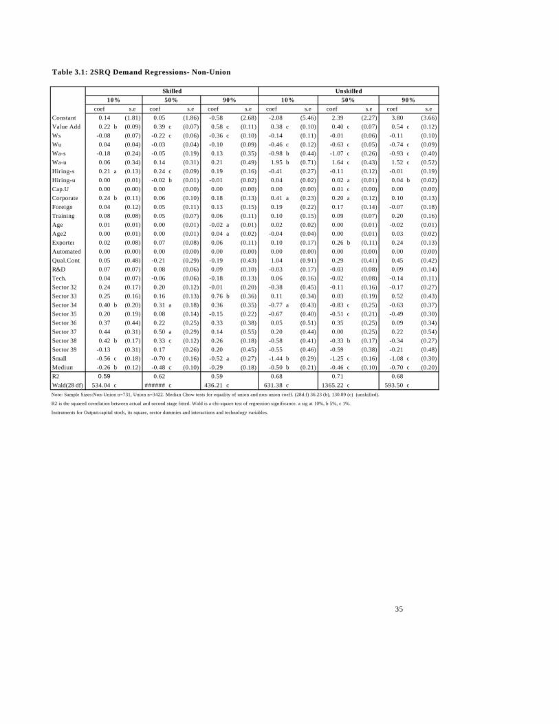
Table 3.1: 2SRQ Demand Regressions- Non-Union

coef s.e coef s.e coef s.e coef s.e coef s.e coef s.eConstant 0.14 (1.81) 0.05 (1.86) -0.58 (2.68) -2.08 (5.46) 2.39 (2.27) 3.80 (3.66)Value Add. 0.22 b (0.09) 0.39 c (0.07) 0.58 c (0.11) 0.38 c (0.10) 0.40 c (0.07) 0.54 c (0.12)Ws -0.08 (0.07) -0.22 c (0.06) -0.36 c (0.10) -0.14 (0.11) -0.01 (0.06) -0.11 (0.10)Wu 0.04 (0.04) -0.03 (0.04) -0.10 (0.09) -0.46 c (0.12) -0.63 c (0.05) -0.74 c (0.09)Wa-s -0.18 (0.24) -0.05 (0.19) 0.13 (0.35) -0.98 b (0.44) -1.07 c (0.26) -0.93 c (0.40)Wa-u 0.06 (0.34) 0.14 (0.31) 0.21 (0.49) 1.95 b (0.71) 1.64 c (0.43) 1.52 c (0.52)Hiring-s 0.21 a (0.13) 0.24 c (0.09) 0.19 (0.16) -0.41 (0.27) -0.11 (0.12) -0.01 (0.19)Hiring-u 0.00 (0.01) -0.02 b (0.01) -0.01 (0.02) 0.04 (0.02) 0.02 a (0.01) 0.04 b (0.02)Cap.U. 0.00 (0.00) 0.00 (0.00) 0.00 (0.00) 0.00 (0.00) 0.01 c (0.00) 0.00 (0.00)Corporate 0.24 b (0.11) 0.06 (0.10) 0.18 (0.13) 0.41 a (0.23) 0.20 a (0.12) 0.10 (0.13)Foreign 0.04 (0.12) 0.05 (0.11) 0.13 (0.15) 0.19 (0.22) 0.17 (0.14) -0.07 (0.18)Training 0.08 (0.08) 0.05 (0.07) 0.06 (0.11) 0.10 (0.15) 0.09 (0.07) 0.20 (0.16)Age 0.01 (0.01) 0.00 (0.01) -0.02 a (0.01) 0.02 (0.02) 0.00 (0.01) -0.02 (0.01)Age2 0.00 (0.01) 0.00 (0.01) 0.04 a (0.02) -0.04 (0.04) 0.00 (0.01) 0.03 (0.02)Exporter 0.02 (0.08) 0.07 (0.08) 0.06 (0.11) 0.10 (0.17) 0.26 b (0.11) 0.24 (0.13)Automated 0.00 (0.00) 0.00 (0.00) 0.00 (0.00) 0.00 (0.00) 0.00 (0.00) 0.00 (0.00)Qual.Cont. 0.05 (0.48) -0.21 (0.29) -0.19 (0.43) 1.04 (0.91) 0.29 (0.41) 0.45 (0.42)R&D 0.07 (0.07) 0.08 (0.06) 0.09 (0.10) -0.03 (0.17) -0.03 (0.08) 0.09 (0.14)Tech. 0.04 (0.07) -0.06 (0.06) -0.18 (0.13) 0.06 (0.16) -0.02 (0.08) -0.14 (0.11)Sector 32 0.24 (0.17) 0.20 (0.12) -0.01 (0.20) -0.38 (0.45) -0.11 (0.16) -0.17 (0.27)Sector 33 0.25 (0.16) 0.16 (0.13) 0.76 b (0.36) 0.11 (0.34) 0.03 (0.19) 0.52 (0.43)Sector 34 0.40 b (0.20) 0.31 a (0.18) 0.36 (0.35) -0.77 a (0.43) -0.83 c (0.25) -0.63 (0.37)Sector 35 0.20 (0.19) 0.08 (0.14) -0.15 (0.22) -0.67 (0.40) -0.51 c (0.21) -0.49 (0.30)Sector 36 0.37 (0.44) 0.22 (0.25) 0.33 (0.38) 0.05 (0.51) 0.35 (0.25) 0.09 (0.34)Sector 37 0.44 (0.31) 0.50 a (0.29) 0.14 (0.55) 0.20 (0.44) 0.00 (0.25) 0.22 (0.54)Sector 38 0.42 b (0.17) 0.33 c (0.12) 0.26 (0.18) -0.58 (0.41) -0.33 b (0.17) -0.34 (0.27)Sector 39 -0.13 (0.31) 0.17 (0.26) 0.20 (0.45) -0.55 (0.46) -0.59 (0.38) -0.21 (0.48)Small -0.56 c (0.18) -0.70 c (0.16) -0.52 a (0.27) -1.44 b (0.29) -1.25 c (0.16) -1.08 c (0.30)Medium -0.26 b (0.12) -0.48 c (0.10) -0.29 (0.18) -0.50 b (0.21) -0.46 c (0.10) -0.70 c (0.20)R2 0.59 0.62 0.59 0.68 0.71 0.68Wald(28 df) 534.04 c ###### c 436.21 c 631.38 c 1365.22 c 593.50 cNote: Sample Sizes:Non-Union n=731, Union n=3422. Median Chow tests for equality of union and non-union coeff. (28d.f) 36.23 (b), 130.89 (c) (unskilled).

R2 is the squared correlation between actual and second stage fitted. Wald is a chi-square test of regression significance. a sig at 10%, b 5%, c 1%.

Instruments for Output:capital stock, its square, sector dummies and interactions and technology variables.

35

Skilled Unskilled10% 50% 90% 10% 50% 90%

Table 3.2: 2SRQ Demand Regressions-Union

coef s.e coef s.e coef s.e coef s.e coef s.e coef s.eConstant 0.56 (0.93) 1.75 b (0.85) 4.11 c (1.46) 1.28 (1.58) 3.73 (0.90) 5.82 b (1.54)Value Add. 0.42 c (0.03) 0.46 c (0.03) 0.53 c (0.04) 0.35 c (0.04) 0.40 c (0.03) 0.43 c (0.04)Ws -0.23 c (0.03) -0.34 c (0.03) -0.51 c (0.04) -0.04 (0.04) -0.02 (0.03) -0.03 (0.03)Wu 0.08 c (0.02) 0.02 (0.02) -0.04 (0.03) -0.58 c (0.03) -0.62 c (0.02) -0.64 c (0.03)Wa-s -0.19 a (0.11) -0.04 (0.10) -0.18 (0.17) 0.31 b (0.15) 0.08 c (0.10) 0.25 b (0.12)Wa-u 0.05 (0.16) -0.07 (0.15) 0.17 (0.27) -0.17 (0.26) -0.15 c (0.17) -0.49 a (0.27)Union -0.19 a (0.11) -0.27 (0.33) -0.95 (0.48) 2.45 c (0.53) 2.59 c (0.38) 2.98 c (0.53)Hiring-s 0.11 a (0.06) 0.10 b (0.05) 0.06 (0.06) -0.07 (0.07) 0.08 (0.04) 0.12 (0.08)Hiring-u 0.00 (0.01) 0.01 a (0.01) 0.01 (0.01) 0.01 (0.01) 0.00 a (0.01) 0.00 b (0.01)Cap.U. 0.00 b (0.00) 0.00 (0.00) 0.00 (0.00) 0.01 c (0.00) 0.00 c (0.00) 0.00 (0.00)Corporate 0.04 (0.04) 0.07 b (0.03) 0.08 (0.06) 0.10 b (0.04) 0.06 a (0.03) 0.01 (0.06)Foreign 0.12 b (0.05) 0.17 c (0.04) 0.20 c (0.06) -0.04 (0.06) -0.01 (0.05) 0.09 (0.06)Training 0.01 (0.04) -0.02 (0.03) -0.04 (0.05) -0.04 (0.04) -0.03 (0.03) -0.01 (0.04)Age 0.00 (0.00) 0.01 b (0.00) 0.00 (0.00) 0.00 (0.00) 0.00 (0.00) 0.00 (0.00)Age2 0.00 (0.00) -0.01 a (0.00) 0.00 (0.01) 0.00 (0.01) 0.01 (0.00) 0.01 b (0.01)Exporter 0.03 (0.05) 0.03 (0.03) 0.06 (0.05) 0.17 c (0.05) 0.23 b (0.04) 0.26 c (0.06)Automated 0.00 (0.00) 0.00 (0.00) 0.00 (0.00) 0.00 a (0.00) 0.00 (0.00) 0.00 (0.00)Qual.Cont. -0.11 (0.26) -0.08 (0.23) 0.10 (0.35) 0.12 (0.22) 0.15 (0.33) -0.26 (0.53)R&D 0.09 b (0.04) 0.03 (0.03) 0.03 (0.05) 0.00 (0.05) -0.03 (0.03) -0.05 (0.05)Tech. -0.02 (0.04) -0.01 (0.03) -0.05 (0.04) -0.02 (0.05) -0.05 (0.03) -0.02 (0.05)Sector 32 0.06 (0.08) 0.10 (0.06) 0.04 (0.11) 0.06 (0.09) 0.23 (0.07) 0.21 b (0.09)Sector 33 0.33 c (0.09) 0.26 c (0.08) 0.03 (0.13) 0.19 (0.11) 0.13 (0.08) 0.06 (0.12)Sector 34 0.17 a (0.10) 0.36 c (0.09) 0.19 (0.14) -0.12 a (0.13) 0.04 c (0.09) 0.12 (0.13)Sector 35 0.30 c (0.08) 0.33 c (0.06) 0.11 (0.11) -0.04 (0.11) 0.00 c (0.06) 0.04 (0.11)Sector 36 0.46 c (0.10) 0.44 c (0.07) 0.23 b (0.11) 0.23 b (0.09) 0.11 (0.08) 0.06 (0.09)Sector 37 0.35 c (0.11) 0.28 c (0.08) 0.10 (0.14) -0.04 (0.10) -0.02 (0.11) 0.03 (0.14)Sector 38 0.35 c (0.07) 0.39 c (0.06) 0.25 b (0.12) 0.06 (0.11) 0.16 b (0.06) 0.34 c (0.11)Sector 39 0.03 (0.14) 0.09 (0.12) -0.12 (0.28) -0.03 (0.14) 0.01 (0.13) -0.01 (0.12)Small -0.44 c (0.08) -0.53 c (0.08) -0.65 c (0.12) -1.30 c (0.10) -1.09 c (0.07) -1.08 c (0.10)Medium -0.25 c (0.05) -0.33 c (0.04) -0.52 c (0.07) -0.56 c (0.06) -0.56 c (0.04) -0.76 c (0.06)R2 0.62 0.63 0.62 0.67 0.68 0.67Wald (29df) 1967.53 c ###### c ###### c 3204.40 c 4210.45 c 3651.45 cNote: Sample Sizes:Non-Union n=731, Union n=3422. Median Chow tests for equality of union and non-union coeff. (28d.f) 36.23 (b), 130.89 (c) (unskilled).

R2 is the squared correlation between actual and second stage fitted. Wald is a chi-square test of regression significance. a sig at 10%, b 5%, c 1%.

Instruments for Output:capital stock, its square, sector dummies and interactions and technology variables.

Skilled Unskilled10% 50% 90% 10% 50% 90%

37

Appendix 1: Measures to Confront the Problem of RecentlyTrained Workers Who Resign, %

Total Large Medium Small MicroIncrease wages 23.1 7.1 7.6 9.5 29.2Increase other remunerations 4.6 17.5 17 14 0.1Promote those trained 12.7 39.6 32.8 24.3 6.1Reduce the # of those trained 8.4 0.2 1.3 1.3 11.5Reduce the training offered 0.2 0.5 0 0 0.3Give non-monetary recognition 8.5 12.8 9.8 7.3 8.4None 33.5 15.5 26.1 35 34.7Don't know 1.2 2.3 0.7 5.2 0Others 7.8 3.9 4.1 3.2 9.7Source: 1992 ENESTYC

38

Appendix 2: OLS Estimates

Table A2.1 – WAGE EQUATIONSNon-union Union

Skilled Unskilled Skilled UnskilledPrd 0.036 (0.028) 0.097 (0.025) a 0.036 (0.012) a 0.039 (0.012) aLwa 0.384 (0.156) a 0.388 (0.204) b 0.300 (0.057) a 0.433 (0.086) aUnion --- --- --- --- -0.865 (0.210) a 0.236 (0.197)Hirr -0.002 (0.090) -0.014 (0.010) -0.065 (0.029) a -0.002 (0.004)Sch 0.424 (0.081) a 0.235 (0.103) a 0.571 (0.058) a 0.238 (0.055) aSch2 -0.016 (0.003) a -0.017 (0.007) a -0.022 (0.002) a -0.014 (0.004) aExp -0.021 (0.023) 0.000 (0.015) 0.027 (0.007) a 0.018 (0.006) aExp2 0.001 (0.001) 0.000 (0.001) -0.001 (0.000) a -0.001 (0.000) aR_d 0.121 (0.065) b 0.004 (0.064) 0.010 (0.025) -0.035 (0.026)Tech. 0.030 (0.063) 0.078 (0.061) 0.097 (0.024) a 0.135 (0.026) aP.train. 0.197 (0.067) a 0.110 (0.065) b 0.024 (0.025) 0.001 (0.026)Corp -0.038 (0.081) -0.008 (0.079) 0.028 (0.026) 0.067 (0.028) aForg. 0.327 (0.096) a 0.127 (0.093) 0.179 (0.030) a 0.025 (0.032)Export. -0.123 (0.074) b 0.012 (0.073) -0.108 (0.026) a 0.024 (0.028)Auto 0.001 (0.001) 0.001 (0.001) 0.001 (0.000) b 0.000 (0.001)Cmptl -0.013 (0.055) 0.026 (0.054) -0.008 (0.022) -0.003 (0.023)Qual.ctr. 0.083 (0.248) -0.193 (0.242) 0.094 (0.186) 0.238 (0.197)LogK/L 0.001 (0.019) -0.026 (0.018) 0.016 (0.008) b -0.014 (0.008) bSect_32 0.046 (0.110) 0.072 (0.101) -0.008 (0.043) -0.028 (0.042)Sect_33 -0.018 (0.143) 0.094 (0.126) 0.063 (0.068) 0.075 (0.069)Sect_34 0.129 (0.134) 0.200 (0.156) 0.072 (0.056) 0.103 (0.063)Sect_35 0.162 (0.124) 0.059 (0.132) 0.116 (0.044) A 0.061 (0.047)Sect_36 0.142 (0.194) -0.006 (0.183) 0.079 (0.060) 0.078 (0.061)Sect_37 0.226 (0.233) -0.192 (0.227) -0.011 (0.065) -0.068 (0.064)Sect_38 0.035 (0.102) 0.107 (0.110) 0.085 (0.038) A 0.065 (0.042)Sect_38 -0.503 (0.256) b -0.045 (0.250) 0.031 (0.090) 0.117 (0.094)Medium -0.132 (0.077) b -0.085 (0.075) -0.229 (0.025) A -0.091 (0.026) aSmall -0.702 (0.083) a -0.349 (0.082) a -0.676 (0.032) A -0.335 (0.033) aConst. 2.912 (1.500) b 3.943 (1.643) a 3.523 (0.680) A 3.082 (0.732) a

R2 0.3987 0.1692 0.2895 0.1191F – test 17.26 a 5. 30 a 49.43 a 16.39 aNote: Sample sizes: Non-union n=731, Union, n=3,422. Chow tests for equality of union and non-union coeff.(27d.f.) 86.66 a (skilled), 42.37 a (unskilled). a-significant at the 5% level, b-significant at the 10% level.

39

Table A2.2 – LABOR DEMAND EQUATIONS – 2SLSNon-union Union

Skilled Unskilled Skilled UnskilledLq * 0.441 (0.039) a 0.493 (0.049) a 0.480 (0.018) a 0.405 (0.019) aLws -0.252 (0.038) a -0.082 (0.047) b -0.379 (0.019) a -0.024 (0.020)Lwu -0.057 (0.036) -0.636 (0.045) a 0.037 (0.016) a -0.591 (0.017) aLwas -0.044 (0.174) -1.028 (0.219) a -0.091 (0.073) 0.195 (0.079) aLwau 0.094 (0.255) 1.423 (0.320) a -0.002 (0.121) -0.244 (0.132) bUnion --- --- --- --- -0.417 (0.243) b 2.689 (0.264) aHirrs 0.237 (0.078) a -0.154 (0.098) 0.081 (0.033) a 0.067 (0.036) bHirru -0.008 (0.009) 0.036 (0.011) a 0.008 (0.004) a 0.001 (0.004)Capu -0.001 (0.001) 0.004 (0.002) a -0.001 (0.001) b 0.003 (0.001) aCorp 0.154 (0.068) a 0.190 (0.086) a 0.080 (0.025) a 0.059 (0.027) aForg 0.068 (0.082) 0.124 (0.104) 0.155 (0.029) a 0.010 (0.032)Age 0.002 (0.005) -0.003 (0.006) 0.004 (0.002) a -0.003 (0.002)Age2 0.004 (0.007) 0.003 (0.009) -0.002 (0.002) 0.008 (0.003) aExport 0.056 (0.064) 0.233 (0.081) a 0.068 (0.026) a 0.234 (0.028) aAuto 0.001 (0.001) 0.001 (0.001) 0.000 (0.000) 0.000 (0.000)Qual.ctr. -0.215 (0.209) 0.253 (0.263) -0.060 (0.176) 0.048 (0.192)R_d 0.073 (0.055) -0.001 (0.070) 0.042 (0.024) b -0.039 (0.026)Tech. -0.064 (0.054) -0.020 (0.068) -0.016 (0.023) -0.027 (0.025)Sect_32 0.200 (0.106) b -0.115 (0.134) 0.075 (0.045) b 0.182 (0.049) aSect_33 0.344 (0.120) a 0.161 (0.151) 0.228 (0.065) a 0.163 (0.071) aSect_34 0.370 (0.148) a -0.647 (0.186) a 0.292 (0.065) a 0.010 (0.071)Sect_35 0.056 (0.114) -0.456 (0.143) a 0.283 (0.049) a -0.025 (0.053)Sect_36 0.268 (0.164) 0.166 (0.207) 0.370 (0.058) a 0.150 (0.063) aSect_37 0.368 (0.199) b 0.064 (0.250) 0.253 (0.061) a 0.016 (0.067)Sect_38 0.361 (0.101) a -0.331 (0.128) a 0.371 (0.046) a 0.177 (0.050) aSect_38 0.057 (0.223) -0.319 (0.280) 0.100 (0.088) 0.003 (0.096)Medium -0.396 (0.076) a -0.528 (0.095) a -0.339 (0.030) a -0.612 (0.033) aSmall -0.611 (0.109) a -1.207 (0.136) a -0.524 (0.050) a -1.129 (0.054) aConst. 0.484 (1.538) a 3.789 (1.934) b 1.986 (0.690) a 3.212 (0.752) a

R2 0.6518 0.6872 0.6339 0.6918F –test 46.77 a 59.47 a 210.25a 269.56 aDHW 32.52 a 19.68 a 72.44 a 151.53 aNote: Sample sizes: Non-union n=731, Union, n=3,422. Chow tests for equality of union and non-union coeff.(26d.f.) 36.23b (skilled), 130.89 a (unskilled). a-significant at the 5% level, b-significant at the 10% level. * Instruments for output: capitalstock, its square, sector dummies and its interactions and technology variables.

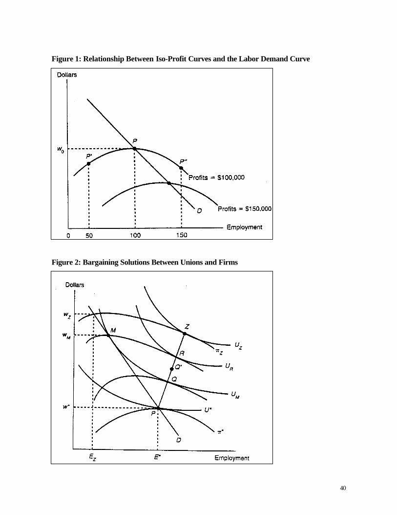
40

Figure 1: Relationship Between Iso-Profit Curves and the Labor Demand Curve

Figure 2: Bargaining Solutions Between Unions and Firms

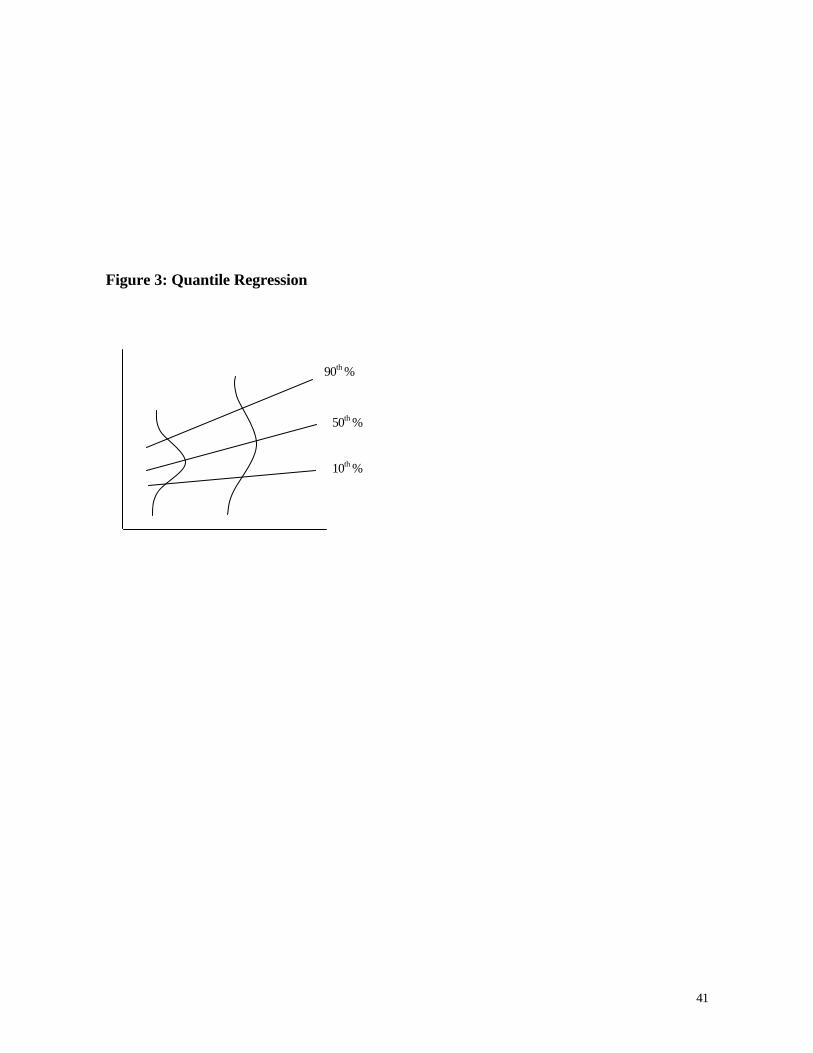
41

Figure 3: Quantile Regression

90th %

50th %

10th %

42

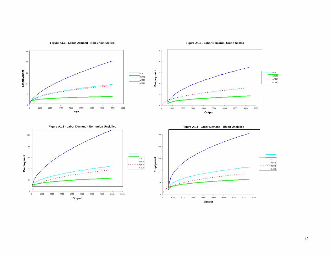
Figure A1.1 - Labor Demand - Non-union Skilled

0

5

10

15

20

25

0 1000 2000 3000 4000 5000 6000 7000 8000 9000

Output

Em

plo

ymen

t

OLS

rq(.10)

rq(.50)

rq(.90)

Figure A1.2 - Labor Demand - Union Skilled

0

5

10

15

20

25

0 1000 2000 3000 4000 5000 6000 7000 8000 9000

Output

Em

plo

ymen

t

OLS

rq(.10)

rq(.50)

rq.(90)

Figure A1.3 - Labor Demand - Non-union Unskilled

0

36

72

108

144

180

0 1000 2000 3000 4000 5000 6000 7000 8000 9000

Output

Em

plo

ymen

t

OLS

rq(.10)

rq(.50)

rq.(90)

Figure A1.4 - Labor Demand - Union Unskilled

0

36

72

108

144

180

0 1000 2000 3000 4000 5000 6000 7000 8000 9000

Output

Em

ply

men

tOLS

rq(.10)

rq(.50)

rq.(90)

42

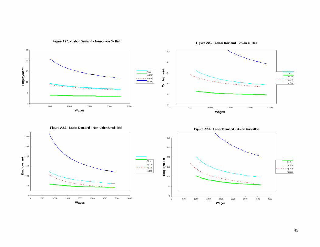
Figure A2.2 - Labor Demand - Union Skilled

0

5

10

15

20

25

0 5000 10000 15000 20000 25000

Wages

Em

plo

ymen

t

OLS

rq(.10)

rq(.50)

rq.(90)

Figure A2.3 - Labor Demand - Non-union Unskilled

0

50

100

150

200

250

300

0 500 1000 1500 2000 2500 3000 3500 4000

Wages

Em

plo

ymen

t

OLS

rq(.10)

rq(.50)

rq.(90)

Figure A2.4 - Labor Demand - Union Unskilled

0

50

100

150

200

250

300

0 500 1000 1500 2000 2500 3000 3500 4000

Wages

Em

plo

ymen

tOLS

rq(.10)

rq(.50)

rq.(90)

Figure A2.1 - Labor Demand - Non-union Skilled

0

5

10

15

20

25

0 5000 10000 15000 20000 25000

Wages

Em

plo

ymen

t

OLS

rq(.10)

rq(.50)

rq.(90)

43