DPRIETI Discussion Paper Series 16-E-054

Efficiency of the Retail Industry:Case of inelastic supply functions

KONISHI YokoRIETI

NISHIYAMA YoshihikoKyoto University

The Research Institute of Economy, Trade and Industryhttp://www.rieti.go.jp/en/

1

RIETI Discussion Paper Series 16-E-054

March 2016

Efficiency of the Retail Industry: Case of inelastic supply functions*

KONISHI Yoko

Research Institute of Economy, Trade and Industry

NISHIYAMA Yoshihiko

Kyoto University

Abstract

We propose a method to measure the efficiency of the retail industry. In the case of the

manufacturing industry, we can define its efficiency by total factor productivity (TFP) based on the

production function. Since retailers do not produce specific objects, we cannot observe their output

with the exception of monetary observations such as sales or profit. TFP could be computed as in the

manufacturing industry using such data, however, increased TFP does not necessarily indicate

efficiency gain for retailers because it also includes the effects from the demand side. If demand

increases, the TFP of retailers will increase. Therefore, we look at retailers' cost function rather than

production function to study their efficiency. Assuming that the retail industry is competitive, we

construct a cost model and identify the cost efficiency. In standard economic theory, duality holds

for productivity and cost efficiency, though it is not clear in the present case. This paper deals with

the retailers of goods with an inelastic supply function which include agricultural and marine

products. We propose and apply a new empirical method to measure the retail industry efficiency of

agricultural products using Japanese regional panel data of wholesale and market prices and traded

quantity for a variety of vegetables from 2008 to 2014. The marginal cost efficiency was stable

during this period.

Keywords: Retail industry, Agricultural products, Cost function, Marginal cost efficiency, Prefectural level data

JEL classification: L81, D24, Q11

RIETI Discussion Papers Series aims at widely disseminating research results in the form of professional

papers, thereby stimulating lively discussion. The views expressed in the papers are solely those of the

author(s), and neither represent those of the organization to which the author(s) belong(s) nor the Research

Institute of Economy, Trade and Industry.

*This study is conducted as a part of the project“Decomposition of Economic Fluctuations for Supply and Demand Shocks: Service industries” undertaken at RIETI. The authors appreciate invaluable advice and comments for data construction by Mr. Takashi Saito (METI). The authors are also grateful for helpful comments and suggestions by Professor Kyoji Fukao (Hitotsubashi University, RIETI-PD), Vice President Masayuki Morikawa (RIETI), President and CRO Masahisa Fujita (RIETI), Naohito Abe (Hitotsubashi University) and seminar participants at RIETI. This research was partially supported by the Ministry of Education, Culture, Sports, Science and Technology (MEXT), Grant-in-Aid for Scientic Research (No. 15K03407 and 15H03335 ) and Research Project 2015 of Kyoto Institute of Economic Research.

1 Introduction

Productivity/efficiency is an important issue in economics because it is considered a source

of economic growth. In the case of manufacturing industry, there exist a large body of litera-

ture, most of which estimates the production function and computes total factor productivity

(TFP) as a measure of productivity. However, relatively little research has been conducted

that studies the productivity of the service or non-manufacturing industries. There are two

essential difficulties relative to manufacturing industry if we take the TFP-type approach to

this problem. First, it is not clear what the service sector produces. For example, the sales

quantity may be considered as the production output, but it also could be regarded as the

input. Therefore, the definition of the production function of the service industry is not a

straightforward issue. One possibility is considering the sales or value-added as the outcome

of service industries. However, this output depends also on the demand. Second, the con-

sumption of service industry is realized only when demand arrives. For example, a hairdresser

serves only when a customer visits the hair salon. Manufactures can produce goods without

demand arrival. If the production quantity exceeds the demand, the stock simply increases.

Productivity is a characteristic of suppliers, and in principle, should not depend on demand.

The purpose of this paper is to measure efficiency of the retail industry. One possible

approach, as stated above, is to compute TFP taking sales, margin, or profit as the outcome.

This is, needless to say, an important measure of industry performance. However, this mea-

sure is affected by consumers’ demand shocks, producers’ supply shocks, retailers’ efficiency

shocks, and input market shocks. This means that it is unclear what kind of policy should

be implemented—demand side, supply side, or retailer efficiency improving—in response to

a decline in TFP in the retail industry. In order to identify the retailers’ efficiency based on

the TFP, we adopt the cost function approach for the efficiency measure related to the role

of retailers. They operate if there is a difference between the market-clearing price and the

price at which they buy goods from suppliers. If the retail industry is competitive, which is

likely, their profit must be zero. We estimate the cost function and cost efficiency of retailers

2

by using this relationship. The retail industry is a part of the service industry. There are

some empirical results of productivity measures for the service industry. We refer to a lim-

ited number of results in this field. Foster et al. (2006) compute the labor productivity of

the retail industry in USA. Kainou (2009) computes labor productivity using Japanese data.

Fukao (2010) computes TFP for various service sectors in Japan by focusing on the effect of

ICT investment. Jorgenson, Nomura and Samules (2015) compare TFP of Japanese and US

wholesale/retail industries to conclude that the former attains only 70% productivity of the

latter. Kwon and Kim (2008) calculate the TFP of the wholesale and retail industry using

Japanese panel data to examine the source of changes in the productivity of the Japanese

wholesale and retail industry. Mas and Moretti (2009) investigate the efficiency of cashier

workers using high frequency data. Morikawa (2011, 2012, 2014) studies the productivity of

a variety of service industries by TFP analysis. Fukao et al. (2016) discuss the results in

connection with the choice of deflator in several service sectors for the UK, US, and Japan.

Konishi and Nishiyama (2010) estimate efficiency of hairdressers using microdata by a hedonic

approach.

In modern microeconometrics, we often apply structural econometric modeling. There, we

construct an economic model of behavior of agency as well as the constitution and market

regulations. In constructing the econometric model, we add shocks and errors, clearly spec-

ifying who can observe which components, which in turn determines how the solutions are

affected. This addresses any problems of endogeneity that may arise. Based on this model, we

study how we can identify quantities of interest and estimate them. This approach is called

structural econometric modeling (see Reiss and Wolak (2007) and Ackerberg, Benkard, Berry

and Pakes (2007) for overviews). In terms of efficiency analysis, Marshack and Andrews (1944)

first identified the endogeneity problem in the production function estimation. Taking this

problem into account, Levinsohn and Petrin (1999, 2003) and Olley and Pakes (1996) proposed

new identification and estimation methods for measuring productivity. Ichimura, Konishi and

Nishiyama (2011), Ackerberg, Caves and Frazer (2015) and many other papers are related to

3

this problem. See the references in these articles. We also refer to Ackerberg et al. (2007) and

Syverson (2010) for a brief survey of this field. We follow this approach to handle the problem

of endogeneity, define, and estimate the efficiency of retailers. The following section provides

a simple economic model of retailer behavior when the supply function is inelastic. Using

this framework, we add shocks and errors to determine the endogeneity structure in Section

3. Section 4 presents an econometric model and its estimation method. Section 5 explains

the data and provides results of the empirical analysis using prices and quantity of Japanese

agricultural products. Section 6 concludes.

2 A simple economic model of retailer and producer behavior

We propose an economic model of retailer behavior based on the key observation that their

profit depends on the price gap between the wholesale and retail markets. There are three par-

ticipants in this setup: consumers, producers, and retailers. Retailers exist because consumers

cannot purchase goods directly from the producers for several reasons. The retailers purchase

goods from the producers in the wholesale market and sell them to consumers observing their

demand function. Needless to say, retailers seek to earn a profit from the price gap. They

have to pay labor and capital costs out of the income from the price gap, which includes wages

and rent for the store and/or warehouse. Retailers are willing to work only when their costs

do not exceed the earnings from the price gap. If the retail industry is competitive, retailers

earn no profit. Then the equilibrium price in the wholesale market will be set at the level at

which the revenue equals the total cost.

In this paper, we consider retailers trading goods with inelastic supply curves, such as

agricultural products. The products, like fresh food, cannot be stocked. Producers supply a

fixed amount of their product to a wholesale market. The supply amount is initially fixed;

thereafter the wholesale price is determined such that the entire supply is sold out. The fixed

supply level, the consumers demand function, and the retailers’ cost determine the wholesale

market price. Producers will determine their optimal supply in the wholesale market such

4

that their revenue is maximized, given the behavior of the retailers. We do not consider the

profit maximization by the producers as the production quantity was already determined in

the past. For example, farmers decide how much cabbage they plant several months before

they sell their crop in the market. They can only adjust how much cabbage they ship in a day

or a month. They cannot ship more than they have, but can choose to dispose a part of the

crop. Under this setup, we obtain a Nash equilibrium in the market.

In the real economy, retailers vary in terms of their scale or other attributes, such as de-

partment stores, supermarkets, and local shops. Obviously, they operate on different principles

and perhaps face different customers. We should carefully construct an economic model that

considers such aspects, especially when we consider commodities with product differentiation.

In this paper, we ignore these issues by using data of ordinary agricultural products. We only

briefly look at the scale effect in the empirical section later.

2.1 Decision of retailers

We present a basic formal model in the above-mentioned framework. See Figure 1.

Suppose producer supply is fixed at q+. The supply function is, units of their products in

the wholesale market, which means that the supply curve is inelastic. For example, farmers

dispatch a certain amount of agricultural products to the wholesale market that must be sold

within the day. The supply function is,

q = q+

as shown in the figure. Let the consumer demand function be

p = α− βq, α > 0, β > 0.

If consumers can directly buy goods from the producers, A is the equilibrium point and the

equilibrium price is pm. Since this is impossible in the present setting, retailers purchase the

5

Figure 1: Equilibrium

pSupply:��

A

Demand:�

B

q

6

products at a certain price pw that is lower than pm and sell them to consumers at pm. pw

is determined by the game played by producers and retailers where producers move first and

supply q+ units of the good. Thereafter, each retailer offers a price. If there is only one

monopolistic retailer, s/he can offer pw = 0. On the other hand, if the retail industry is

competitive, pw will be determined such that the revenue pmq+ equals the total cost of the

retailers, thereby implying zero retailers’ profit. It seems likely that retailers compete with

each other, as the barriers to entry in the retail industry are not significant, except in case of

some special commodities. Let the cost of retailers exclusive of purchase cost be

C(q) = c0 + c1q.

Retailers need to pay C(q) to sell the quantity q of the commodity. This consists of labor

costs, capital costs, and other costs like transportation costs. c0, c1 depend on such input

prices, but we do not explicitly outline this relationship now. The total cost including the

purchase cost is C(q) + pwq.

Retailers operate only when

(pm − pw)q+ ≥ c0 + c1q+

and the retailers’ purchase price must satisfy

pw ≤ (pm − c1)− c0

q+

= (α− βq+ − c1)− c0

q+.

The equality uses the equilibrium condition of retail market.

7

2.2 Nash Equilibrium under perfect competition in retail industry

If the retail industry is competitive, or the no profit condition holds, the retailers offer the

price

pw = (α− βq+ − c1)− c0

q+.

Based on this retailer behavior, rational suppliers determine the supply quantity q+ such that

pwq+ is maximized. Let Q be the maximum quantity that they can supply. Their optimization

problem is

maxq+

pwq+ s.t. q+ ≤ Q, pw ≤ (α− βq+ − c1)− c0

q+.

Q depends on factors such as the farmers’ ex-ante demand expectation and weather. When

Q ≥ α−c1

2β , the supply constraint q+ ≤ Q is not binding. If the market is competitive, the

solution is

q∗ =α− c1

2β

which gives the equilibrium prices

pm∗ = α− α− c1

2=

α+ c1

2,

pw∗ =α− c1

2− 2βc0

α− c1

and the revenue for the producers is

R∗ = pw∗q∗ =(α− c1)2

4β− c0 (1)

If suppliers behave rationally, they control q+ as above. Thereafter, suppliers dispose the

amount Q − α−c1

2β and sell only α−c1

2β units of the product. Thus the amount traded in the

market is endogenous. However, the amount traded can be exogenous in some cases, such

8

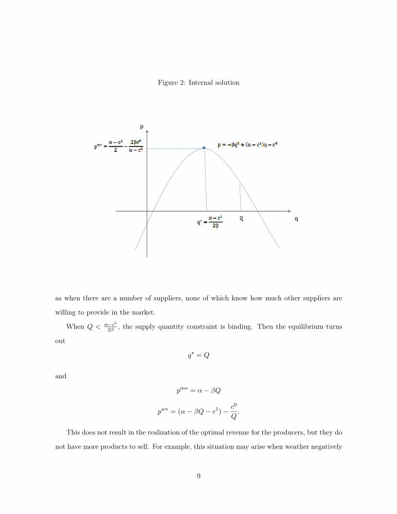
Figure 2: Internal solution

p

q

as when there are a number of suppliers, none of which know how much other suppliers are

willing to provide in the market.

When Q < α−c1

2β , the supply quantity constraint is binding. Then the equilibrium turns

out

q∗ = Q

and

pm∗ = α− βQ

pw∗ = (α− βQ− c1)− c0

Q.

This does not result in the realization of the optimal revenue for the producers, but they do

not have more products to sell. For example, this situation may arise when weather negatively

9

Figure 3: Corner solution

p

q

affects the crop. Figures 2 and 3 show the cases where the supply quantity constraint is

binding, and is not binding, respectively.

If the retail industry is not competitive, pw can be smaller than pw∗ depending on the

possibility of competitiveness and collusion.

2.3 Subsidy to product disposal

Government subsidizes product disposal due to abundant crop to keep the price in a certain

range and protect producers. This could affect the optimization behavior of producers. More

specifically, producers could earn more by disposing more than the optimal amount of product

if the subsidy is too high. We briefly see the effect of such a scheme. We consider the case

when Q > q∗ so that producers provide q∗ in the market and dispose amount Q− q∗ if there

is no subsidy. Suppose government subsidizes τ per unit of disposed product when pw is too

10

small, say pw < p. When producers provide q unit of products in the market and dispose

Q− q, the revenue is

R = pwq + τ(Q− q)1(pw < p)

where

pw = (α− βq − c1)− c0

q.

The producers will choose q such that

maxq

R =

−βq2 + (α− c1)q − c0 if − βq2 + (α− c1 − p)q − c0 > 0

−βq2 + (α− c1 − τ)q − c0 + τQ otherwise

When producers can earn more by disposing more than the optimal amount of product, con-

sumer utility falls. The supply is insufficient when

R∗ < (p− τ)q1 + τQ

where q1 = {(α− c1 − p)−√

(α− c1 − p)2 − 4βc0}/2β. If Q is bounded, which is likely, it is

possible to set p and τ such that the above inequality holds. Therefore, the government can

provide a subsidy scheme such that the supplied quantity remains q∗ and thus, the price does

not unnecessarily rise.

3 Shocks, endogeneity and efficiency

We construct an econometric model based on the economic model presented in the previous

section. We need to make explicit assumptions about shocks and errors in the equations. This

step clarifies the kind of endogeneity, heterogeneity, heteroscedasticity, and other econometric

aspects being considered. We also define efficiency measures in this setup.

11

3.1 Shocks and endogeneity

We specify the market demand function as

p = α− βq + uS + uR + uSR + u (2)

where uS and uR are shocks that can only be observed by the suppliers and the retailers,

respectively. uSR is the shock that can be observed by both suppliers and retailers and u is

the unobservable error. We assume the retailers cost function to be

C = c0 + (c1 + v1S + v1R + v1SR + v1)q + v0S + v0R + v0SR + v0 (3)

where the superscripts S, R, SR indicate the same as described in the case of the shocks.

The superscripts 0 and 1 mean that the shocks correspond to the constant and the slope,

respectively. v0, v1 are external errors. c0 and c1 are components which depend on input

prices so that, if the relationship is linear,

c0 = γ0 + γ1r + γ2w + γ3g

c1 = δ0 + δ1r + δ2w + δ3g

where r is the price of capital, w is wage per hour and g is the petrol price.

Taking the same line as in section 2 with a special attention to who can observe which

shocks, we determine the optimizing behaviors. We first look at the decision of retailers.

Retailers can only observe part of (2) and (3), or the demand function

p = α− βq + uR + uSR

12

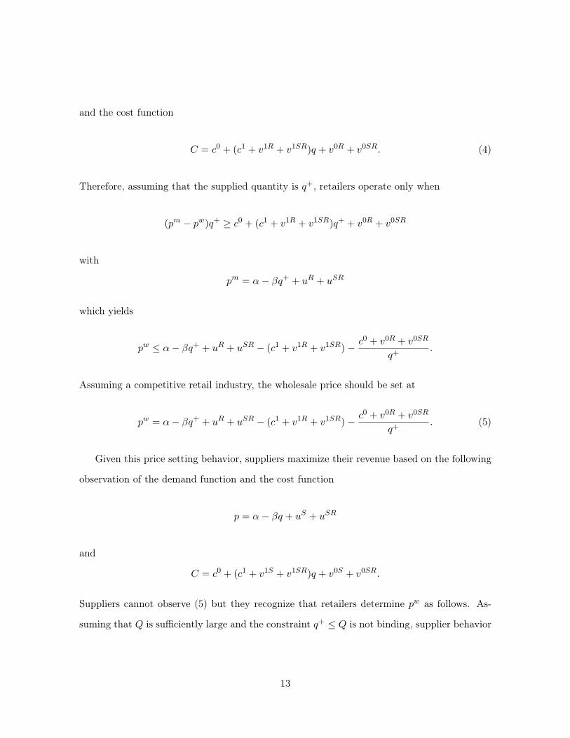
and the cost function

C = c0 + (c1 + v1R + v1SR)q + v0R + v0SR. (4)

Therefore, assuming that the supplied quantity is q+, retailers operate only when

(pm − pw)q+ ≥ c0 + (c1 + v1R + v1SR)q+ + v0R + v0SR

with

pm = α− βq+ + uR + uSR

which yields

pw ≤ α− βq+ + uR + uSR − (c1 + v1R + v1SR)− c0 + v0R + v0SR

q+.

Assuming a competitive retail industry, the wholesale price should be set at

pw = α− βq+ + uR + uSR − (c1 + v1R + v1SR)− c0 + v0R + v0SR

q+. (5)

Given this price setting behavior, suppliers maximize their revenue based on the following

observation of the demand function and the cost function

p = α− βq + uS + uSR

and

C = c0 + (c1 + v1S + v1SR)q + v0S + v0SR.

Suppliers cannot observe (5) but they recognize that retailers determine pw as follows. As-

suming that Q is sufficiently large and the constraint q+ ≤ Q is not binding, supplier behavior

13

is characterized by

maxq+

pwq+ s.t. pw = α− βq+ + uS + uSR − (c1 + v1S + v1SR)− c0 + v0S + v0SR

q+.

This gives

q∗ =α+ uS + uSR − c1 − v1S − v1SR

2β.

Based on the above results, the realized quantity and prices are

q = min(q∗, Q)

pm = α− βq + uS + uR + uSR + u

pw = α− βq + uR + uSR − (c1 + v1R + v1SR)− c0 + v0R + v0SR

q.

Therefore, in terms of observed quantity and prices, we have

(pm − pw)q = (c1 + uS + u+ v1R + v1SR)q + (c0 + v0R + v0SR) (6)

= c0 + c1q + ϵ

where

ϵ = (uS + u+ v1R + v1SR)q + (v0R + v0SR).

3.2 Efficiency of retailers

In the above model, the demand function is determined by consumers and the supply level

is determined by the producers based on revenue maximization. All retailers can do is to

determine the wholesale price based on the cost function. If a retailer is a monopolist, s/he can

set the wholesale price to be arbitrarily small. If the industry is competitive, the wholesale price

must be set at (5). In the case of oligopoly, the wholesale price must be somewhere between

14

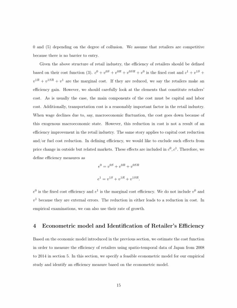
0 and (5) depending on the degree of collusion. We assume that retailers are competitive

because there is no barrier to entry.

Given the above structure of retail industry, the efficiency of retailers should be defined

based on their cost function (3). c0 + v0S + v0R + v0SR + v0 is the fixed cost and c1 + v1S +

v1R + v1SR + v1 are the marginal cost. If they are reduced, we say the retailers make an

efficiency gain. However, we should carefully look at the elements that constitute retailers’

cost. As is usually the case, the main components of the cost must be capital and labor

cost. Additionally, transportation cost is a reasonably important factor in the retail industry.

When wage declines due to, say, macroeconomic fluctuation, the cost goes down because of

this exogenous macroeconomic state. However, this reduction in cost is not a result of an

efficiency improvement in the retail industry. The same story applies to capital cost reduction

and/or fuel cost reduction. In defining efficiency, we would like to exclude such effects from

price change in outside but related markets. These effects are included in c0, c1. Therefore, we

define efficiency measures as

e0 = v0S + v0R + v0SR

e1 = v1S + v1R + v1SR.

e0 is the fixed cost efficiency and e1 is the marginal cost efficiency. We do not include v0 and

v1 because they are external errors. The reduction in either leads to a reduction in cost. In

empirical examinations, we can also use their rate of growth.

4 Econometric model and Identification of Retailer’s Efficiency

Based on the economic model introduced in the previous section, we estimate the cost function

in order to measure the efficiency of retailers using spatio-temporal data of Japan from 2008

to 2014 in section 5. In this section, we specify a feasible econometric model for our empirical

study and identify an efficiency measure based on the econometric model.

15

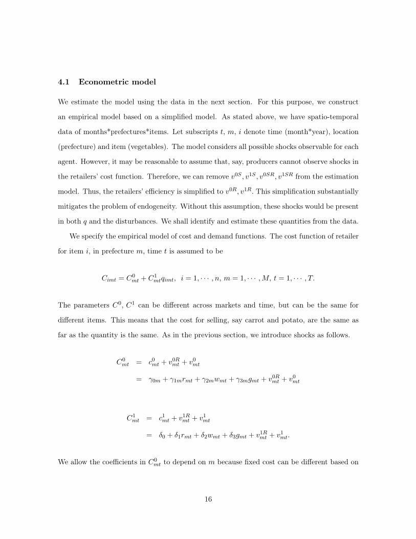
4.1 Econometric model

We estimate the model using the data in the next section. For this purpose, we construct

an empirical model based on a simplified model. As stated above, we have spatio-temporal

data of months*prefectures*items. Let subscripts t, m, i denote time (month*year), location

(prefecture) and item (vegetables). The model considers all possible shocks observable for each

agent. However, it may be reasonable to assume that, say, producers cannot observe shocks in

the retailers’ cost function. Therefore, we can remove v0S , v1S , v0SR, v1SR from the estimation

model. Thus, the retailers’ efficiency is simplified to v0R, v1R. This simplification substantially

mitigates the problem of endogeneity. Without this assumption, these shocks would be present

in both q and the disturbances. We shall identify and estimate these quantities from the data.

We specify the empirical model of cost and demand functions. The cost function of retailer

for item i, in prefecture m, time t is assumed to be

Cimt = C0mt + C1

mtqimt, i = 1, · · · , n, m = 1, · · · ,M, t = 1, · · · , T.

The parameters C0, C1 can be different across markets and time, but can be the same for

different items. This means that the cost for selling, say carrot and potato, are the same as

far as the quantity is the same. As in the previous section, we introduce shocks as follows.

C0mt = c0mt + v0Rmt + v0mt

= γ0m + γ1mrmt + γ2mwmt + γ3mgmt + v0Rmt + v0mt

C1mt = c1mt + v1Rmt + v1mt

= δ0 + δ1rmt + δ2wmt + δ3gmt + v1Rmt + v1mt.

We allow the coefficients in C0mt to depend on m because fixed cost can be different based on

16

the market size. For each market and time, we can define the retailers’ efficiency by

e0mt = γ0m + v0Rmt , e1mt = δ0 + v1Rmt (7)

.

Given this specification, we estimate the model

(pmimt − pwimt)qimt = C0mt + C1

mtqimt

= c0mt + (c1mt + uSimt + uimt + v1Rmt)qimt + v0Rmt + v0mt

= c0mt + c1mtqimt + ϵimt (8)

where

c0mt = γ0m + γ1mrmt + γ2mwmt + γ3mgmt

c1mt = δ0 + δ1rmt + δ2wmt + δ3gmt

ϵimt = (uSimt + uimt + v1Rmt)qimt + v0Rmt + v0mt (9)

qimt = min(q∗imt, Qimt)

q∗imt =α+ uSimt + uSRimt − c1mt

2β.

The demand function of item i, in prefecture m, time t is

pmimt = αmt − βmtqimt + κiImt + uSimt + uRimt + uSRimt + uimt (10)

where Imt is the income of prefecture m at time t. We assume that its coefficient depends on

only the product; this implies that the utility function does not change over time.

17

4.2 Estimation of Efficiency

Our main target is to extract the efficiency measures in (7). For this purpose, we use equations

(8) and (10) in the previous section with suitable instruments. In view of q and the disturbance

structure, uSimt+uSRimt turns out the source of endogeneity. As it is a part of the demand shock,

we can use climate variable Z as the instrument to consistently estimate the parameters. Z

consists of the average temperature, average rainfall, and average hours of sunlight. Formally,

we assume that

E{(v1Rmt + v1mt)qimt + v0Rmt + v0mt|Zmt} = 0

E(uSimt + uRimt + uSRimt + uimt|Zmt) = 0

We estimate the model by the Generalized Method of Moments (GMM) to obtain γ0m, γ1m,

γ2m , γ3m, δ0, δ1, δ2, δ3, αmt, βmt, κi and the residuals

ϵimt = (pmimt − pwimt)qimt − (c0mt + c1mtqimt)

where

c0mt = γ0m + γ1mrmt + γ2mwmt + γ3mgmt

c1mt = δ0 + δ1rmt + δ2wmt + δ3gmt.

Based on (9), ϵimt estimates (uSimt + uimt + v1Rmt)qimt + v0Rmt + v0mt. Assuming demand shocks

uSimt, uimt are independent of lagged quantity qim,t−1, we propose to estimate v1Rmt by

v1Rmt = (n∑

i=1

qim,t−1qimt)−1

n∑i=1

qim,t−1ϵimt.

We need some other information to identify v0Rmt .

18

5 Data and Empirical results

Our research objective is the examination of the efficiency of retailers that sell goods with

inelastic supply such as agricultural products. For this purpose, we estimate eq. (8) with

suitable instruments for quantities (qimt). Using the estimation results, we identify efficiency

by eq. (7). Due to the restriction of data, some shocks are removed from the model as noted

in section 4. Therefore, our analysis is limited to being based on a simplified model. In this

section, we present variable descriptions, summary statistics of variables, and the estimation

results.

5.1 Data

We collect spatio-temporal data of months*prefectures*items conducted by Japanese min-

istries that are available online. Let subscripts t, m, i denote time (month*year), location

(prefecture) and item (vegetables) in (8); the subscript y denotes year in Table 1. Table 1

describes the variables used in the empirical analysis and the sources from which the data

for the variables is obtained. The dataset is composed of 47 prefectures, 27 vegetables, 12

months, and 7 years (2008–2014), which accounts for more than 100,000 observations. The

selected vegetables are Japanese radish, carrot, burdock lotus root, Chinese cabbage, cabbage,

spinach, Welsh onion, asparagus, broccoli, lettuce, cucumber, pumpkin, eggplant, tomato,

green pepper, string bean, green soybean, sweet potato, potato, taro, Japanese yam, onion,

ginger, shiitake mushroom, enoki mushroom, and shimeji mushroom. Table 2 shows the sum-

mary statistics of the dependent variable ((pmimt − pwimt)qimt), the explanatory variables (wmy,

rmy, gmt) and the instrumental variables (Z: tempmt, sunnymt, rainmt) for qimt in (8). We

deflate monetary base data by using a consumer price index (deflator1mt) and a consumer

prices index (deflator2my) of regional difference.

19

Tab

le1:

Var

iabl

eD

escr

ipti

ons

and

Sour

ces

ofD

ata

vari

able

(uni

t)D

escr

ipti

onSo

urce

spw im

t(y

en)

Who

lesa

leW

hole

sale

pric

eSu

rvey

onV

eget

able

san

dFr

uits

Who

lesa

leM

arke

t,pr

ice

Min

istr

yof

Agr

icul

ture

,For

estr

yan

dFis

heri

esq imt(k

g)W

hole

sale

Who

lesa

lepr

ice

Surv

eyon

Veg

etab

les

and

Frui

tsW

hole

sale

Mar

ket,

quan

tity

Min

istr

yof

Agr

icul

ture

,For

estr

yan

dFis

heri

espm im

t(ye

n)R

etai

lR

etai

lPri

ceSu

rvey

(Str

uctu

ralS

urve

y),

pric

eM

inis

try

ofIn

tern

alA

ffair

san

dC

omm

unic

atio

nswmy(y

en)

Ave

rage

wag

era

teB

asic

Surv

eyon

Wag

eSt

ruct

ure,

ofre

tail

indu

stry

Min

istr

yof

Hea

lth,

Labo

uran

dW

elfa

rer m

y(y

en/m

2)

the

valu

eof

com

mer

cial

dist

rict

sM

inis

try

ofLa

nd,I

nfra

stru

ctur

e,Tra

nspo

rtan

dTou

rism

g mt(

yen)

Ligh

ter

fluid

’sPet

role

umP

rodu

cts

Pri

ceSt

atis

tics

,av

erag

epr

ice

Min

istr

yof

Eco

nom

y,Tra

dean

dIn

dust

rytempmt(

C)

Ave

rage

tem

pera

ture

sunny m

t(ho

urs)

Suns

hine

dura

tion

(Tot

alam

ount

)Ja

pan

Met

eoro

logi

calA

genc

y,ra

inmt(m

m)

Rai

nfal

lM

inis

try

ofLa

nd,I

nfra

stru

ctur

e,Tra

nspo

rtan

dTou

rism

(Tot

alam

ount

)field

yt(ha)

area

offie

ldfo

rSt

atis

tics

onC

rop,

vege

tabl

esM

inis

try

ofA

gric

ultu

re,F

ores

try

and

Fis

heri

esdef

lator1

mt

pric

ein

dex

Con

sum

erP

rice

Indi

ces,

All

item

sba

seye

ar=

2010

Min

istr

yof

Inte

rnal

Affa

irs

and

Com

mun

icat

ions

def

latr2 m

yre

gion

aldi

ffere

nce

The

Reg

iona

lDiff

eren

ceIn

dex

ofC

onsu

mer

Pri

ces,

All

item

spr

ice

inde

xM

inis

try

ofIn

tern

alA

ffair

san

dC

omm

unic

atio

ns

20

Table 2: Summary Statistics (2008-2014)variable (unit) unit mean median S.D. min. max. N(pmimt − pwimt)qimt yen 95220 34567 218780.3 5.9 4619603 102277pwimt yen 347.1 280.6 270.1 18.3 2395.4 102279qimt ton 496.5 135 1288.9 1 25600 102279pmimt yen 695.3 564.5 511.7 60.3 4345.9 102279fieldyt ha 24838.7 9190 59697.6 1370 414900 102279wmy yen 261470.6 261157.2 26811.2 193124.1 373870.6 102279rmy yen/m2 144371.3 85018.6 203512.4 27569.05 1602426 102279gmt yen 125.6 128.1 15.0 87.6 172.6 102279tempmt C 15.6 15.9 8.5 -4.7 30.5 102279sunnymt hours 161.5 163.2 45.8 17.6 294.4 102279rainmt mm 142.9 114.5 113.3 0 1561 102279

5.2 Empirical Results

In order to observe the efficiency of retailers, we estimate eq. (8) considering the problems of

endogeneity and heterogeneity, as stated in section 3. We implement 2SLS regression to handle

the problem of endogeneity in qimt by using the prefecture level monthly climate data, such

as average temperature, duration of sunshine, and total amount of rainfall, as instrumental

variables. Figure 4 shows the aggregated quantities by prefectures in 2014 and the cumulative

curves. Ten prefectures (from Rank 1 to 10) occupied more than 60% of the sum of quantities

of 47 prefectures, which indicates to the existence of heterogeneity in the quantities. We

consider to control the differences of market scale among prefectures. Therefore, we adopted

(qimt/fieldyt) as the dependent variable in the first stage regression, and regressed qimt/fieldyt

on climate variables. Table 3 shows the result of first stage regression; we obtained adjusted

R2 = 0.498 and found that coefficients of average temperature, lag of average temperature,

and duration of sunny hours are positive and significant. The coefficient of the square of

average temperature is negative and significant. Due to limited data availability, we simplify

eq. (8) for estimation to

(pmimt − pwimt)qimt = C0m + C1

y qimt + ϵimt. (11)

21

We examine the fitted values of qimt that are calculated by ˆqimt = qimt/fieldyt × fieldyt

using the estimation results of first step. We allow the coefficients in C0m to depend on each

prefecture. Therefore, C0m captures the difference in market size between prefectures. In eq.

(8), C1mt that stands for marginal cost has subscripts time*prefectures. However, we assume

that C1depends only on year in eq. (11). Due to the serious multicollinearity problem, we

choosed a subscriot y as the better expression of marginal cost. Both C0m and C1

y do not have

a subscript i in eq. (11). This is because we assume that the cost for selling the same quantity

of, say carrots and potatoes, are the same. As a second step, we estimate the cost function

for 100,670 observations and obtain the adjusted R2=0.70. In the interest of saving space, we

only check the signs of the fitted values of eq. (11) and do not present the estimation results

of all coefficients. As C0m+C1

y qimt denotes the total cost, we expect that estimation results of

C0m +C1

yˆqimt to be positive value. In figure 5, we calculated average of C0

m + C1yˆqimt in terms

of year and items for each prefecture and the averages are positive. Additionally, we observed

that the retailers in big cities tend to spend higher expenses to sell vegetables.

Using estimation results of eq. (11), we obtain residuals ϵimt = (pmimt − pwimt)qimt − (c0mt +

c1mtqimt). According to eq. (9), we can rewrite the residuals as ϵimt = (uSimt+uimt+v1Rmt)qimt+

v0Rmt + v0mt. v0mt and v1Rmt are components of fix cost efficiency (e0) and marginal cost efficiency

(e1) in eq. (7), respectively. Assuming that the demand shocks of uSimt and uimt are indepen-

dent of lagged quantityqim,t−1, we proposed to estimation of v1Rmt by

v1Rmt = (

n∑i=1

qim,t−1qimt)−1

n∑i=1

qim,t−1ϵimt.

We can obtain v1Rmt by implementing GMM estimation of ϵimt on qimt, the instrumental

variables of qimt are qim,t−1. However, it is not able to be identify v0Rmt without additional

information. Figure 6 shows the average marginal cost efficiency every year, and the bar

graph of each year indicates the cost of selling an additional 1 kg of vegetables. When the

cost decreases, the marginal cost efficiency improves (and vice versa). The solid and dotted

22

line plots represent mean ± 1σ and mean ± 2σ; these lines tell us whether the average of

each year changes or not. As a result, each bar is located in the confidence intervals, which

suggests that the marginal cost efficiency was stable for these seven years in Japan. Finally, we

observe the relation between the marginal cost efficiency and the regional features of retailers

in the “Yearbook of the Current Survey of Commerce, 2014” conducted by the Ministry of

Economy, Trade, and Industry. We aggregate v1Rmt in each prefecture and examine the corre-

lation coefficients with each index. We found that prefectures that have a high establishment

ratio of small and medium size establishments have lower marginal cost efficiency. On the

other hand, when the share of large business is higher in a prefecture, the efficiency tends to

be higher. When shopping floor per person is larger, the efficiency is lower. The shop floor

productivity is defined by total amount sales over number of employees, and the correlation

between productivity and efficiency is positive. Moreover, the labor productivity is defined by

total amount sales over number of employees, and the correlation between labor productivity

and efficiency is insignificant. It suggests that measuring labor productivity is not enough to

know the efficiency of selling vegetables.

23

Figure 4: qimt(Right), Cumulative curve of qimt(Left), 2014

24

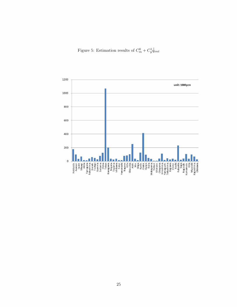
Figure 5: Estimation results of C0m + C1

yˆqimt

25

Table 3: Estimation Result: First Stage

qimt/field

tempmt 1.241∗∗∗

(0.451)

sunnymt 0.045∗

(0.024)

rainmt 0.014(0.016)

temp2mt -0.061∗∗∗

(0.013)

rain2mt -0.000

(0.000)

tempmt−1 0.550∗∗∗

(0.193)

sunnymt−1 -0.020(0.024)

rainmt−1 0.001(0.009)

constant -46.366∗∗∗

(9.287)N 100670R2 0.498

1. 1. Prefecture dummy and year dummy are included.2. 2. Vegetables dummy are included.3. 3. Standard errors in parentheses∗ p < 0.1, ∗∗ p < 0.05, ∗∗∗ p < 0.01

26

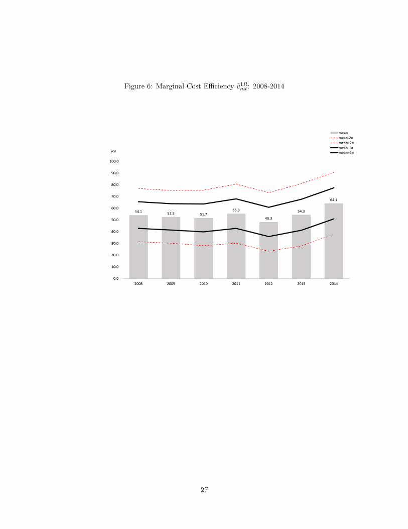
Figure 6: Marginal Cost Efficiency v1Rmt : 2008-2014

27

Table 4: The Correlation between v1Rmt and Retailer’s Indices

Indices Retail Industry (all) Efficiency** p< 0.05 (when each index is higher)

the Share of small business 0.31** lower(≦ 4 employees)the Share of small business 0.37** lower(≦ 10 employees)the Share of large business -0.46** higher(50 ≦ employees <100 )the Share of large business -0.33** higher(≧ 100 employees)Floor space per person 0.41** lowerShop floor productivity -0.28** higherLabor Productivity -0.04 no relation

Source of indices: “Yearbook of the Current Survey of Commerce (2014)” conducted byMinistory of Economy, Trade and Industry.

6 Concluding remarks

We proposed an economic model of retailers and constructed an econometric model based on

it. The basic idea is to describe retailers’ behavior as buying goods at a price and then selling

them at a higher price. They do not operate if the cost of their business cannot be recovered.

In this paper, we look at goods with an inelastic supply, such as agricultural and marine

products. Market price is determined by consumer demand and quantity supplied; thus there

is no room for retailers to affect the price in principle. Retailers can only decide the price to

offer to suppliers, or wholesale price. If the retail industry is competitive, the wholesale price

will be set such that revenue from the price difference equals the retailers’ cost. Based on

such behavior of retailers, suppliers will optimize the amount of supply in the market. Such

interaction determines the market price, the wholesale price, and the quantity traded. We

add shocks to the demand function and retailers’ cost function to define the retailers’ cost

efficiency and determine the structure of endogeneity. We estimate this econometric model

by the IV method to obtain the parameters and the retailers’ efficiency using agricultural

products transaction data in Japan.

28

Our method is novel in that we define the efficiency carefully such that the measure is

not contaminated by demand and supply shocks. It is obvious that the efficiency measure

will be affected by such shocks if we compute TFP using sales or profit data to estimate the

production function. In our empirical analysis, we compute the trend of retailers’ efficiency

for each prefecture and we aggregate them to determine retailers’ efficiency in Japan.

It may be interesting to measure efficiency of each retailer, unlike aggregated efficiency that

is calculated in this paper. The proposed method does not directly apply in the estimation of

efficiency of a retailer who sells multiple goods. If we have a detailed microdata of market and

wholesale prices and quantities of each item, it can be similarly determined. The measurement

of the efficiency of different kinds of retailers, such as department stores, supermarkets, and

local shops is important. These problems will be handled in future research. Moreover, most

goods have elastic supply functions; therefore, methods that are applicable to such goods need

to be developed. Research that does this is currently underway.

References

[1] Ackerberg, D., C. L. Benkard, S. Berry, and A. Pakes (2007) “Econometric Tools for

Analyzing Market Outcomes,” Handbook of Econometrics, Vol. 6A, 4171-4276.

[2] Ackerberg, D., K. Caves and G. Frazer (2015) “Identification Properties of Recent Pro-

duction Function Estimators,” Econometrica, Vol. 83, No. 6, 2411-2451.

[3] Foster, L., J. Haltiwanger, C.J. Krizan (2006) “Market selection, reallocation, and re-

structuring in the US retail trade sector in the 1990s,” The Review of Economics and

Statistics 88 (4), 748-758.

[4] K. Fukao (2010) “Service Sector Productivity in Japan: The key to future economic

growth,” RIETI-PDP series 10-P-007.

29

[5] Fukao, K., T. Kameda, K. Nakamura, R. Namba, M. Sato and S. Sugiura (2016) “Mea-

surement of Deflators and Real Value Added in the Service Sector,” mimeo.

[6] Ichimura, H., Y. Konishi and Y. Nishiyama (2011) “An Econometric Analysis of Firm

Specific Productivities: Evidence from Japanese plant level data,” RIETI-DP series, 11-

E-002.

[7] Jorgenson, D.W., K. Nomura and Jon D. Samuels (2015) “A Half Century of Trans-Pacific

Competition: Price level indices and productivity gaps for Japanese and U.S. industries,

1955-2012,” RIETI-DP series 15-E-054.

[8] K. Kainou (2009) “kakei syohi to tiiki kouri service gyo no cyoki kozo henka,” RIETI-DP

Series 09-J-014.

[9] Konishi, Y., and Y. Nishiyama (2010) “Productivity of Service Providers: Microecono-

metric measurement in the case of hair salons,” RIETI-DP series, 10-E-51.

[10] Kwon H. U., and Y. G. Kim (2008) “nihon no syogyo ni okeru seisansei dynamics-kigyo

katsudo kihon cyosa kohyo data niyoru jissyo bunseki,” RIETI-DP Series 08-J-058.

[11] Levinsohn, J and A. Petrin (2003), “Estimating production functions using inputs to

control for unobservables,” Review of Economic Studies, 70 (2) , 317-411.

[12] Levinsohn, J. and A. Petrin (1999), “When industries become more productive, do firms?:

investigating productivity dynamics,” NBER working paper series; working paper 6893;

Cambridge: National Bureau of Economic Research.

[13] Mas, A. and E. Moretti (2009) “Peers at Work,” American Economic Review, vol. 99-1,

112-145.

[14] Marschak, J. and W.H. Andrews (1944), “Random Simultaneous Equations and the The-

ory of Production,” Econometrica, vol 12, 143-205.

30

[15] M. Morikawa (2014) Service sangyo no seisansei bunseki, Nihon hyoron sha.

[16] M. Morikawa (2012) “Demand Fluctuations and Productivity of Service Industries,” Eco-

nomics Letters, Vol. 117, No. 1, pp. 256-258, 2012.

[17] M. Morikawa (2011) “Economies of Density and Productivity in Service Industries: An

Analysis of Personal Service Industries Based on Establishment-Level Data,” Review of

Economics and Statistics, Vol. 93, No. 1, pp. 179-192, 2011.

[18] Olley, G., S. and A. Pakes (1996), “The dynamics of productivity in the telecommunica-

tions equipment Industry,” Econometrica, vol. 64, 1263-1297.

[19] Reiss, P.C., and F.A. Wolak (2007) “Structural Econometric Modelling: Rationale and

Examples from Industrial Organizations” Handbook of Econometrics, Vol. 6A, 4277-4415.

[20] C. Syverson (2011) “What Determines Productivity?” Journal of Economic Literature,

49:2, 326–365.

31