Embed Size (px)
Citation preview
EFFICIENCY IMPROVEMENTS OFRANS-BASED ANALYSIS AND
OPTIMIZATION USING IMPLICITAND ADJOINT METHODS ON
UNSTRUCTURED GRIDS
A thesis submitted to the University of Manchesterfor the degree of Doctor of Philosophy
in the Faculty of Engineering and Physical Sciences
2006
Richard P. DwightSchool of Mathematics

2
Contents
Abstract 6
Declaration 7
Copyright 8
Acknowledgements 9
1 Introduction 111.1 Implicit Time Stepping Methods . . . . . . . . . . . . . . . . . . . . . 12
1.1.1 Literature Review . . . . . . . . . . . . . . . . . . . . . . . . . 141.1.2 Overview . . . . . . . . . . . . . . . . . . . . . . . . . . . . . 15
1.2 The Adjoint Method of Flow Sensitivities . . . . . . . . . . . . . . . . 16
2 Discretization and Jacobians 192.1 Introduction . . . . . . . . . . . . . . . . . . . . . . . . . . . . . . . . 192.2 The Navier-Stokes Equations . . . . . . . . . . . . . . . . . . . . . . . 20
2.2.1 The Instantaneous Equations . . . . . . . . . . . . . . . . . . 202.2.2 The Favre Averaged Equations . . . . . . . . . . . . . . . . . 22
2.3 Flow Regime . . . . . . . . . . . . . . . . . . . . . . . . . . . . . . . 232.4 Finite Volume Discretization . . . . . . . . . . . . . . . . . . . . . . . 242.5 Construction of the Jacobian . . . . . . . . . . . . . . . . . . . . . . . 262.6 Central Convective Fluxes . . . . . . . . . . . . . . . . . . . . . . . . 28
2.6.1 Scalar Dissipation for the Central Scheme . . . . . . . . . . . 292.6.2 Jacobian of Dissipation under a Constant Coefficient Approxi-
mation . . . . . . . . . . . . . . . . . . . . . . . . . . . . . . . 312.6.3 Full Jacobian of Scalar Dissipation . . . . . . . . . . . . . . . 32
2.7 Gradient Approximation . . . . . . . . . . . . . . . . . . . . . . . . . 352.7.1 Green-Gauss Jacobian . . . . . . . . . . . . . . . . . . . . . . 35
2.8 Viscous Flux Modelling . . . . . . . . . . . . . . . . . . . . . . . . . . 352.8.1 TSL Viscous Flux Derivatives . . . . . . . . . . . . . . . . . . 36
2.9 Solid Wall Boundary Conditions . . . . . . . . . . . . . . . . . . . . . 372.9.1 Slip-Wall . . . . . . . . . . . . . . . . . . . . . . . . . . . . . . 372.9.2 Slip-Wall Jacobians . . . . . . . . . . . . . . . . . . . . . . . . 382.9.3 No-Slip Wall . . . . . . . . . . . . . . . . . . . . . . . . . . . . 382.9.4 No-Slip Wall Jacobians . . . . . . . . . . . . . . . . . . . . . . 38
2.10 Permeable Boundary Conditions . . . . . . . . . . . . . . . . . . . . . 392.10.1 Subsonic Outflow Condition . . . . . . . . . . . . . . . . . . . 41
3
2.11 Turbulence Model Discretization . . . . . . . . . . . . . . . . . . . . . 422.11.1 Expression for the Eddy-Viscosity . . . . . . . . . . . . . . . . 422.11.2 Convective Fluxes . . . . . . . . . . . . . . . . . . . . . . . . . 422.11.3 Diffusion Fluxes . . . . . . . . . . . . . . . . . . . . . . . . . . 432.11.4 Spalart-Allmaras Source Terms . . . . . . . . . . . . . . . . . 432.11.5 Spalart-Allmaras-Edwards Source Terms . . . . . . . . . . . . 442.11.6 Boundary Conditions . . . . . . . . . . . . . . . . . . . . . . . 45
2.12 Summary . . . . . . . . . . . . . . . . . . . . . . . . . . . . . . . . . 45
3 Approximately Factored Implicit Schemes 463.1 Introduction . . . . . . . . . . . . . . . . . . . . . . . . . . . . . . . . 463.2 Description of the Scheme . . . . . . . . . . . . . . . . . . . . . . . . 47
3.2.1 Symmetric Gauss-Seidel (SGS) Solution . . . . . . . . . . . . 483.2.2 Inviscid Flux Jacobians . . . . . . . . . . . . . . . . . . . . . . 503.2.3 Viscous Flux Jacobians . . . . . . . . . . . . . . . . . . . . . . 513.2.4 Turbulence Jacobians . . . . . . . . . . . . . . . . . . . . . . . 523.2.5 Dual-Time Treatment . . . . . . . . . . . . . . . . . . . . . . 55
3.3 Analysis of the Scheme . . . . . . . . . . . . . . . . . . . . . . . . . . 553.3.1 Theoretical Stability Conditions for Fixed-Point Iterations . . 563.3.2 Von Neumann Analysis of the Scheme . . . . . . . . . . . . . 633.3.3 Time-Accuracy of the Scheme . . . . . . . . . . . . . . . . . . 73
3.4 Numerical Results . . . . . . . . . . . . . . . . . . . . . . . . . . . . . 773.4.1 Approximations of the Jacobian . . . . . . . . . . . . . . . . . 773.4.2 Influence of Linear Solver . . . . . . . . . . . . . . . . . . . . 783.4.3 Influence of Viscous Flux Approximation . . . . . . . . . . . . 823.4.4 Influence of Point Ordering . . . . . . . . . . . . . . . . . . . 843.4.5 Parallel Efficiency . . . . . . . . . . . . . . . . . . . . . . . . . 843.4.6 Generic Delta-Wing . . . . . . . . . . . . . . . . . . . . . . . . 853.4.7 Wing-Body-Tail Configuration . . . . . . . . . . . . . . . . . . 88
3.5 Summary . . . . . . . . . . . . . . . . . . . . . . . . . . . . . . . . . 90
4 Unfactored Implicit Schemes 914.1 Introduction . . . . . . . . . . . . . . . . . . . . . . . . . . . . . . . . 91
4.1.1 Overview . . . . . . . . . . . . . . . . . . . . . . . . . . . . . 934.2 Construction of the Exact Jacobian . . . . . . . . . . . . . . . . . . . 944.3 Solution of the Linear System . . . . . . . . . . . . . . . . . . . . . . 95
4.3.1 Application of Existing Non-Linear Iteration . . . . . . . . . . 964.3.2 Application of preconditioned GMRES . . . . . . . . . . . . . 98
4.4 Example of an Exact Newton Method . . . . . . . . . . . . . . . . . . 1024.5 Approximate Newton Methods . . . . . . . . . . . . . . . . . . . . . . 103
4.5.1 1st-Order Jacobian Krylov Implicit Method (FOKI) . . . . . . 1044.5.2 Alternative 1st-Order Implicit Method (FOGSI) . . . . . . . . 1074.5.3 Numerical Comparison of LU-SGS, FOKI and FOGSI . . . . . 108
4.6 Summary . . . . . . . . . . . . . . . . . . . . . . . . . . . . . . . . . 113
4
5 The Discrete Adjoint Equations 1145.1 Introduction . . . . . . . . . . . . . . . . . . . . . . . . . . . . . . . . 114
5.1.1 Overview . . . . . . . . . . . . . . . . . . . . . . . . . . . . . 1165.2 Aerodynamic Design Problem . . . . . . . . . . . . . . . . . . . . . . 116
5.2.1 Details of the Discretization . . . . . . . . . . . . . . . . . . . 1175.3 Gradients via Discrete Adjoint . . . . . . . . . . . . . . . . . . . . . . 117
5.3.1 Primal Approach . . . . . . . . . . . . . . . . . . . . . . . . . 1175.3.2 Adjoint Approach . . . . . . . . . . . . . . . . . . . . . . . . . 1175.3.3 Adjoint of the Grid Deformation . . . . . . . . . . . . . . . . 1185.3.4 Implementation of the Method . . . . . . . . . . . . . . . . . . 119
5.4 Approximations of the Discrete Adjoint . . . . . . . . . . . . . . . . . 1205.4.1 1st-Order Approximation (FOA) . . . . . . . . . . . . . . . . 1205.4.2 Thin Shear-Layer (TSL) Assumption . . . . . . . . . . . . . . 1205.4.3 Constant JST Coefficients Approximation (CCA) . . . . . . . 1215.4.4 Constant Eddy-Viscosity (CEV) Assumption . . . . . . . . . . 1215.4.5 Use of an Alternative Turbulence Model (ATM) . . . . . . . . 122
5.5 Results and Discussion . . . . . . . . . . . . . . . . . . . . . . . . . . 1225.5.1 Transonic RAE2822 Aerofoil . . . . . . . . . . . . . . . . . . . 1235.5.2 Three-Element High-Lift Configuration . . . . . . . . . . . . . 131
5.6 Conclusions . . . . . . . . . . . . . . . . . . . . . . . . . . . . . . . . 135
6 Conclusions 1386.1 Further Work . . . . . . . . . . . . . . . . . . . . . . . . . . . . . . . 140
A Change of Variables 142A.1 Primitive Variables . . . . . . . . . . . . . . . . . . . . . . . . . . . . 142A.2 Alternative Primitive Variables . . . . . . . . . . . . . . . . . . . . . 143A.3 Entropy Variables . . . . . . . . . . . . . . . . . . . . . . . . . . . . . 144A.4 Symmetrizing Variables . . . . . . . . . . . . . . . . . . . . . . . . . . 145A.5 Parabolic Symmetrizing Variables . . . . . . . . . . . . . . . . . . . . 146
References 149
54,000 words total
5
Abstract
The efficiency of an unstructured grid finite volume RANS solver is significantlyimproved using two implicit methods based on differing philosophies. The LU-SGSmultigrid method aims to improve performance, while maintaining the low memoryrequirements and robustness of an explicit scheme. The First-Order Krylov Implicit(FOKI) method sacrifices these to some extent, in order to achieve high convergencerates and also avoid the use of a multigrid method, whilst care is taken that themethod remains practical for large 3d cases. The speeds of the two schemes arecompared with that of an existing, highly-tuned Runge-Kutta multigrid method, andit is seen that a factor of two speed-up can be obtained with no additional memoryoverhead using LU-SGS, and a factor of ten with FOKI. Attention is then turned tothe efficiency of aerodynamic design optimization using gradient-based methods. Useof the Jacobian from the implicit methods allows construction of the adjoint of theflow solver. This adjoint is exact in the sense of being based on the full linearizationof all terms in the solver, including all turbulence model contributions. From thisstarting point various approximations to the adjoint are derived with the intention ofsimplifying the development and reducing the memory requirements of the method.The effect of these approximations on the accuracy of the resulting design gradients,and the convergence and final solution of optimization problems is studied. The resultis a tool for extremely rapid sensitivity evaluations.
6

Declaration
No portion of the work referred to in this thesis has beensubmitted in support of an application for another degreeor qualification of this or any other university or otherinstitution of learning.
7
Copyright
Copyright in text of this thesis rests with the Author. Copies (by any process)either in full, or of extracts, may be made only in accordance with instructions givenby the Author and lodged in the John Rylands University Library of Manchester.Details may be obtained from the Librarian. This page must form part of any suchcopies made. Further copies (by any process) of copies made in accordance with suchinstructions may not be made without the permission (in writing) of the Author.
The ownership of any intellectual property rights which may be described in thisthesis is vested in the University of Manchester, subject to any prior agreement tothe contrary, and may not be made available for use by third parties without thewritten permission of the University, which will prescribe the terms and conditionsof any such agreement.
Further information on the conditions under which disclosures and exploitationmay take place is available from the Head of the Department of Mathematics.
8
Acknowledgements
The task of writing a thesis is not one which can be performed in isolation, andthere are many people who have contributed to this work in ways both tangible andintangible. Foremost amongst the former group must be my friend and colleagueJoel Brezillon, who has made the chapter on the adjoint method possible through hisinsight and experience in optimization, not to mention his dedicated hard work.
Deserving of particular mention are Jens Faßbender and Markus Widhalm forpatiently answering uncountable questions on finite volume schemes, Axel Schwoppefor providing the crash course in Galerkin methods that was a prerequisite for the(abortive) chapter on deformation, as well as Bernard Eisfeld, Antonio Fazzolari,Ralf Hartmann, Cord Rossow, Joachim Held and Ralf Heinrich for many inspiringand productive discussions. Advice from Ken Badcock and Mark Woodgate from theUniversity of Glasgow was extremely helpful during initial efforts in constructing theJacobian.
To Norbert Kroll and all my colleagues in the Numerical Methods department atthe DLR Braunschweig I owe thanks for the opportunity to work in such a stimulatingenvironment, as well as for forbearance in the face of my awful German. To myprofessor, Peter Duck I am grateful for proposing this Ph.D. in the first place, andfor performing all the functions of a doctoral supervisor.
Last but not least I would like to thank Krystyna Kurpiers, to whom I owe somuch of the happiness of the last three years, and who was also responsible for thecatchy acronym “FOKI”.
I never knew before what eternity was made for. It is to give someof us a chance to learn German. — Mark Twain
9

10
Chapter 1
Introduction
The efficiency of a Computational Fluid Dynamics (CFD) solver for the compressibleNavier-Stokes (NS) equations is critical to its success as an engineering tool. As fi-nite volume based NS methods have become established in the aircraft design process,they are subject to ever increasing demands on their abilities, from three principaldirections. Firstly there is a requirement for modelling of increasingly complex ge-ometries, which is met through the use of unstructured and hybrid grids. Secondlythere is a demand for more accurate physical modelling, whereby the main area ofinterest is advanced turbulence models such as Reynolds Stress Models (RSM) andunsteady simulation in the form of Detached- and Large-Eddy Simulation (DES andLES). Finally there is a desire to use the existing flow solvers within inner loops forthe purposes of optimization, trimming, and stability and control analysis.
The first two of these requirements have the effect of increasing the cost of in-dividual flow calculations. Experience shows that flow solvers based on structuredgrids can be made significantly more efficient than unstructured grid solvers, partlybecause solution methods, in particular multigrid, are more effective on structuredgrids (Wild, 2004). The cost of improving the physical modelling is even greater.Use of RSM for compressible flow in three-dimensions requires 12 unknown variablesper grid point, as compared to 6 for a one-equation turbulence model, with corre-spondingly increased costs. In addition the resulting equations are extremely poorlyconditioned. On the other hand using DES on a complete aircraft configuration hasonly recently become possible as a research exercise, alone due to the computing re-sources required (Spalart & Bogue, 2003); its use in design may be considered still tobe distant (Johnson et al., 2003).
However high performance is demanded even from stationary RANS calculationswith simple turbulence models, when large numbers of such analyses must be per-formed within an outer optimization loop, for example. For calculations on unstruc-tured grids, performance of the solver is often the bottleneck which prevents the use ofCFD for more complex applications. While computer performance is still improvingexponentially, improvements in algorithmic convergence acceleration are also essen-tial for achieving the desired modelling complexity. In fact some sources note thatimprovements in algorithms over the past 50 years have kept pace with improvementsin computer power over the same period (Mavriplis, 1998)1.
Efficiency of solver algorithms is therefore one of the most critical questions in
1For Poisson’s equation.
11
12 CHAPTER 1. INTRODUCTION
modern CFD, and it will be addressed in the context of finite volume RANS methodsusing one-equation turbulence models in this thesis. In particular the application ofthe class of implicit time stepping methods is considered, see Section 1.1.
For the particular case of aerodynamic design, the high cost of the flow analysismakes gradient-based optimization algorithms attractive. However the evaluation ofthe design gradients is also an expensive operation; this difficulty will be tackled us-ing the adjoint method, see Section 1.2. The resulting performance improvement, incombination with the improvement in the efficiency of the flow solver itself via im-plicit algorithms, are two essential parts of a system which can very rapidly optimizeaerodynamic shapes. This thesis ends with some closing remarks in Chapter 6.
1.1 Implicit Time Stepping Methods
We are concerned with the solution to steady-state of ordinary differential equationsof the form
dWi
dt+Ri(W ) = 0,
where W are the unknowns and R is the non-linear residual resulting from the spatialdiscretization of the RANS equations. In particular we use pseudo time stepping andare interesting in optimizing the convergence of the resulting iteration.
Implicit methods for the above equation are characterized by the presence of theresidual evaluated at the unknown time-level, R(W n+1), creating in general a non-linear algebraic system of equations to be solved for W n+1. The method of resolvingthis system by choosing some linearization of the residual R and thus reducing thenon-linear system to a linear algebraic equation, forms the class of implicit methodsstudied here (the compliment being implicit methods solved at each step using anon-linear sub-iteration, e.g. the dual-time method). A further distinction can bemade between methods that perform the necessary linearization on the continuousgoverning equations, and those that linearize the discretized equations. The laterapproach is much more widely used in CFD, perhaps because it has the advantage ofdecoupling the time and space discretizations (known as the method of lines), therebyallowing relatively independent investigation of each. It is also the approach adoptedhere.
Implicit methods of this sub-class can in turn be classified by three importantchoices made during their formulation:
(a) Temporal discretization formula, e.g. Backward-Difference Formula (BDF).
(b) Choice of approximation of the Jacobian of R.
(c) Solution of the resulting linear system: which solver, to what accuracy etc.?
Consequently, the most well-known implicit method, Newton’s method, is specifiedby: (a) the backward-Euler formula with ∆t → ∞, (b) use of the exact Jacobian ofR, and (c) exact solution of the linear system, whereby the choice of particular linearsolver is of secondary importance.
Evaluation of the exact Jacobian, and solution of the linear system to machine ac-curacy tend to be two extremely expensive operations; as such Newton’s method is one
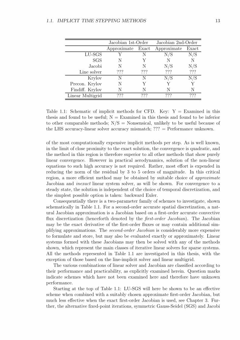
1.1. IMPLICIT TIME STEPPING METHODS 13
Jacobian 1st-Order Jacobian 2nd-OrderApproximate Exact Approximate Exact
LU-SGS Y N N/S N/SSGS N Y N N
Jacobi N N N/S N/SLine solver ??? ??? ??? ???
Krylov N N N/S N/SPrecon. Krylov N Y Y YFindiff. Krylov N N N N
Linear Multigrid ??? ??? ??? ???
Table 1.1: Schematic of implicit methods for CFD. Key: Y = Examined in thisthesis and found to be useful; N = Examined in this thesis and found to be inferiorto other comparable methods; N/S = Nonsensical, unlikely to be useful because ofthe LHS accuracy-linear solver accuracy mismatch; ??? = Performance unknown.
of the most computationally expensive implicit methods per step. As is well known,in the limit of close proximity to the exact solution, the convergence is quadratic, andthe method in this region is therefore superior to all other methods that show purelylinear convergence. However in practical aerodynamics, solution of the non-linearequations to such high accuracy is not required. Rather, most effort is expended inreducing the norm of the residual by 3 to 5 orders of magnitude. In this criticalregion, a more efficient method may be obtained by suitable choice of approximateJacobian and inexact linear system solver, as will be shown. For convergence to asteady state, the solution is independent of the choice of temporal discretization, andthe simplest possible option is taken: backward Euler.
Consequentially there is a two-parameter family of schemes to investigate, shownschematically in Table 1.1. For a second-order accurate spatial discretization, a nat-ural Jacobian approximation is a Jacobian based on a first-order accurate convectiveflux discretization (henceforth denoted by the first-order Jacobian). The Jacobianmay be the exact derivative of the first-order fluxes or may contain additional sim-plifying approximations. The second-order Jacobian is considerably more expensiveto formulate and store, but may also be evaluated exactly or approximately. Linearsystems formed with these Jacobians may then be solved with any of the methodsshown, which represent the main classes of iterative linear solvers for sparse systems.All the methods represented in Table 1.1 are investigated in this thesis, with theexception of those based on the line-implicit solver and linear multigrid.
The various combinations of linear solver and Jacobian are classified according totheir performance and practicability, as explicitly examined herein. Question marksindicate schemes which have not been examined here and therefore have unknownperformance.
Starting at the top of Table 1.1: LU-SGS will here be shown to be an effectivescheme when combined with a suitably chosen approximate first-order Jacobian, butmuch less effective when the exact first-order Jacobian is used, see Chapter 3. Fur-ther, the alternative fixed-point iterations, symmetric Gauss-Seidel (SGS) and Jacobi
14 CHAPTER 1. INTRODUCTION
are shown to be inferior to LU-SGS for the problems considered, unless a much moreaccurate first-order Jacobian is taken. In that case SGS is significantly more efficientthan Jacobi. A line solver has not been investigated here, but is known to be effec-tive, especially for viscous flows (Mavriplis, 1998). All these methods however areineffective in combination with a second-order Jacobian due to the increased stiffnessand reduced diagonal-dominance of the system, as well as the more expensive matrix-vector product. For such a system fixed-point iterations must generally be used incombination with either a Krylov-subspace solver or multigrid on the linear system.
Although it is possible to apply a Krylov method directly to the linear system,indicated by the line “Krylov” in Table 1.1, this technique is generally only effectivefor relatively well-conditioned systems. The only systems that can be described aswell-conditioned are some approximate first-order Jacobian systems, which are laterseen to be more efficiently solved with LU-SGS. Krylov methods preconditioned usingone of the fixed-point iterations described above on the other hand is very generallyapplicable, and widely used in CFD with both first-order Jacobians (Dubuc et al.,1996) and second-order Jacobians (Chisholm & Zingg, 2002). Explicit evaluationand storage of the Jacobian can be avoided using a finite difference approximation,however this tends to be more costly in CPU time than the explicit formulation dueto the number of residual evaluations involved.
The two methods examined in Chapter 4 both use the exact first-order Jacobian,one using an SGS iteration (FOGSI), the other a preconditioned Krylov iteration(FOKI). As can be seen from the table, both prove to be effective methods.
Finally, multigrid in CFD is most often used in the Full-Approximation Storage(FAS) form (Jameson & Baker, 1984), but may also be used inside an implicit methodas a linear solver, a possibility that shows some considerable promise (Mavriplis,2002), but which is not investigated here.
1.1.1 Literature Review
One of the most widely used convergence acceleration algorithms in CFD today wasdescribed in all significant details more than 20 years ago (Jameson & Baker, 1984).The method uses a particularly simple explicit Runge-Kutta (RK) method, wherebythe dissipative part of the convective fluxes is evaluated only at certain RK stages.In addition local time stepping, directional implicit smoothing of the residuals, andFull-Approximation Storage (FAS) multigrid combine to make an extremely effectivescheme. A variant of this method formed the only time stepping scheme of the DLRunstructured RANS solver TAU, up until the work presented in this thesis, and isa highly tuned method, experience in its use having been accumulated over manyyears. The scheme will henceforth be referred to as the Runge-Kutta (RK) method,and will be used as a reference scheme throughout.
Implicit methods with approximate first-order Jacobians and weak linear solversin CFD were first proposed in the context of structured grid methods with implicittreatment of lines in the direction normal to the wall, as presented in (Venkatakrish-nan, 1998) and (Turkel et al., 1999), and the Alternating Direction Implicit (ADI)scheme, in which implicit line treatment in each grid direction is performed (Peaceman& Rachford, 1955). These methods are well known to be unconditionally unstable inthree-dimensions however, leading to a common modification, Diagonally Dominant
1.1. IMPLICIT TIME STEPPING METHODS 15
(DDADI) schemes (Faßbender, 2003).The previous methods are restricted to structured grids, but have been used on
structured parts of mixed-element (hybrid) grids with great success (Mavriplis, 1998),and even time-accurately (Yoh & Zhong, 2004). General unstructured grids requirean alternative solution method, proposed first in CFD for aerodynamics in (Jameson& Turkel, 1981), where a symmetric Gauss-Seidel (GS) sweep was used on a struc-tured grid to solve a heavily approximated linear system. This became known as theLU-SGS (or LU-SSOR) method, and was further developed in (Yoon & Jameson,1986b; Yoon & Jameson, 1988) and more recently in (Luo et al., 1998; Sharov et al.,2000). A method incorporating a modified form of LU-SGS has also been shown, forsimple configurations and a particular discretization, to allow convergence of Eulercomputations within 10 multigrid cycles (Jameson & Caughey, 2001). Also reportedby several sources is that by using a single Jacobi sweep rather than GS, for discretiza-tions including matrix dissipation, a scheme resembling a matrix preconditioner maybe effective (Pierce, 1997; Pierce et al., 1997). Generally all these methods are usedas multigrid smoothers.
Implicit methods with exact first- or second-order Jacobians are less common,possibly due to the considerably greater development effort, and increased memoryrequirements and parallelization problems (Cai et al., 1995). A means of avoidingstorage of the Jacobian is via Jacobian Free Newton-Krylov (JFNK) methods (Knoll& Keyes, 2004), which approximate Jacobian-vector products using finite differences.Zingg and coworkers use an explicitly stored first-order Jacobian to precondition aJFNK method, allowing the use of the very effective ILU method as a precondi-tioner (Chisholm & Zingg, 2002; Wong & Zingg, 2005). Others avoid exact Jacobianscompletely by using a first-order Jacobian in the Newton method (Cantariti et al.,1999; Cantariti et al., 1999), whereby both storage, and effort in the linear system so-lution are saved. The effects of various Krylov solvers on Newton problems resultingfrom CFD has been studied (Meister, 1998), as have the effects of various precon-ditioners. A recently proposed scheme (Rossow, 2005) is one of few to use accurateJacobians and not a Krylov method, but a GS iteration, thereby reducing memoryrequirements.
1.1.2 Overview
Two novel variants of implicit methods are proposed for a spatial discretization in-volving the JST (Jameson et al., 1981) scheme. Throughout this thesis we take twodistinct attitudes to the question of memory requirements of the algorithms. Initiallywe attempt to devise an implicit scheme that uses no more memory than that of theRunge-Kutta, thus allowing it to be a slot-in replacement for that scheme in everysituation. Later we recognize that some increase in memory requirements may beacceptable, and necessary for further improvement in solver performance. Hence thetrade-off between memory and efficiency is explored in some detail.
The first method resembles the LU-SGS method of (Yoon & Jameson, 1988) usedas a multigrid smoother is examined, Chapter 3. The goal is to devise a scheme withall the advantages of Runge-Kutta, i.e. low memory requirements, low computationaleffort per iteration, easy parallelizability, and easy implementation, but that addition-ally admits a high CFL number. The former allows the scheme to function as a slot-in
16 CHAPTER 1. INTRODUCTION
replacement for Runge-Kutta, and thereby admits application to very large test cases.The later will allow faster convergence rates than seen with Runge-Kutta. This isachieved by noting that the Jacobian of the JST scheme takes a very simple form inthe interior of the field, in particular its block diagonal at each point is a multiple ofthe identity matrix. By simplifying the Jacobians of boundary conditions and viscousfluxes this property is preserved, and the approximate Jacobian block diagonal canbe stored with a single floating-point number at each grid point. Inversion is thentrivial, and off-diagonal entries may be rapidly calculated on the fly. The turbulencemodel treatment follows a similar pattern, whereby the mean flow and turbulenceequations are fully decoupled in the Jacobian but calculated simultaneously, allowingrapid matrix and residual evaluation as well as separate treatment.
Comparisons with the highly tuned explicit Runge-Kutta method already de-scribed are undertaken, and the method is found to converge 10-50% faster in termsof iterations, while one LU-SGS iteration costs approximately 90% of one RK itera-tion.
Secondly in Chapter 4 the priorities are changed; a scheme with significantlygreater memory requirements is allowed, but it should perform well without multigrid.The novel scheme developed is denoted the First-Order Jacobian, Krylov Implicit(FOKI) scheme, which is similar to the scheme considered in a structured contextfor upwind discretizations in (Cantariti et al., 1999), but differs in its applicationto unstructured grids and the JST scheme, and in the treatment of the turbulenceequations. The exact Jacobian of the first-order discretization is considered, includ-ing boundary conditions and viscous fluxes. Because the turbulence discretizationincludes only immediate point neighbours in its stencil it is linearized exactly, and issolved decoupled from and independently of the mean flow problem.
The solution method consists of ILU(0) preconditioned GMRES, and convergenceis compared with the LU-SGS scheme of the previous chapter. A factor of 4-5 im-provement in CPU time over that method is recorded for turbulent cases at highReynolds numbers.
1.2 The Adjoint Method of Flow Sensitivities
Given the considerable effort required to evaluate the exact Jacobian of the full finitevolume discretization in order to build a Newton method, as described in Section 4,it is worth considering whether this construction - which amounts to a linearizationof the entire flow solver - may be useful in other contexts. Indeed there are severalpotential applications, and one in particular that promises to be of very considerableuse in the aerodynamic design process, the adjoint method, which has been furtherdeveloped in the context of this thesis, and which is the subject of this chapter.
In aerodynamic design one typically starts from a baseline geometry, a parameter-ization of the shape of the geometry, and a quantity of interest such as aerodynamicdrag on the geometry (the cost function). The objective is to find the choice of coef-ficients of the parameterization (the design variables), such that the cost-function isminimized. Additionally the problem may be subject to one or more constraints.
Two features distinguish aerodynamic design from other design problems. Firstlythe evaluation of the cost-function is typically very expensive, one evaluation corre-sponds to a solution of the Navier-Stokes equations on the given geometry. Secondly,
1.2. THE ADJOINT METHOD OF FLOW SENSITIVITIES 17
because shapes must be parameterized, the problem is often characterized by verylarge numbers of design variables. For two-dimensional design of a profile, 10-30design variables are typical, and when designing a three-dimensional wing severalprofiles and a wing planform may be parameterized, routinely leading to of the or-der of 100 design variables. The optimization problem then consists of a search ina 100-dimensional design space, which combined with the expense of cost-functionevaluations, means that only gradient-based optimization methods are admissible.
Gradient-based optimization characterized by the steepest descent method re-quires two basic steps: first the evaluation of the search direction - the gradient ofthe cost-function with respect to the design variables - which results in the mostrapid improvement of the design locally; and second a one-dimensional search in thisdirection, consisting of repeated evaluations of the cost-function until a minimum isfound in this one-dimensional subspace; this basic process is repeated until no fur-ther improvement is obtained. The derivative of the cost-function with respect to alarge number of design variables is therefore required. The adjoint method providesa means of performing this with an effort only weakly dependent on the number ofdesign variables; the technique is described in detail in Section 5.3.
One of the earliest applications of adjoint methods to aerodynamics problemsis found in the works of Pironneau, who devised optimality conditions for drag ontwo-dimensional bodies, first in Stokes flow (Pironneau, 1973), then for convectiondominated flow (Pironneau, 1974). The work was shortly thereafter applied numer-ically to aerodynamic design (Glowinski & Pironneau, 1975). Effort has since beenapplied to the treatment of increasingly complex problems. Jameson popularized themethod in the aerodynamic community with design of profiles using a continuousadjoint of the Euler equations (Jameson, 1988). Since then a contentious issue hasbeen the choice of continuous or discrete adjoint (Sirkes & Tziperman, 1997). Theformer involves adjointing the continuous equations before discretizing them in orderto solve them numerically (Gauger & Brezillon, 2003; Brezillon & Gauger, 2004);the later adjoints the already discretized equations. Each has advantages, but thediscrete has gained dominance recently, due to its straightforward formulation, andits ability to treat general viscous problems (Nadarajah & Jameson, 2001; Kim et al.,2002). As a result it has become a relatively mature technique (Giles et al., 2003).However recent work suggests a generalization of the continuous adjoint for viscousproblems may be possible (Castro et al., 2006).
Recently (Mavriplis, 2006), building on previous work (Nielsen & Park, 2005;Mavriplis, 2005), showed that by adjointing not only the flow solver, but the entireoptimization chain in a discrete manner, including surface mesh parameterizationand grid deformation, an optimization of the wing of a transport aircraft with anextremely large number of design variables could be performed in less than 6 hourson a standard 16 processor cluster. However, the effort required to develop a discreteadjoint of a given flow solver is very high, as it involves differentiating all partsof the discretization, and often storing the resulting Jacobian matrix (Brezillon &Dwight, 2005). One effort to avoid this overhead uses Automatic Differentiation (AD)tools (Griewank, 2000; Griewank & Walther, 2002), but these are not yet matureenough to be applied to complete flow solvers. Another uses a modified form of finitedifferences in complex variables, and has been applied to large test cases (Nielsen &Kleb, 2005).
18 CHAPTER 1. INTRODUCTION
Here we consider a third approach, which involves using an approximation to theJacobian; a modification which must influence the resulting gradients. Despite thefact that the idea is widely used (Lohner et al., 2003; Soto et al., 2004; Reutheret al., 1999), there have been few studies into its effect on the resulting optimization.Nielsen compared the gradients of several approximations (Nielsen, 1998), and Kim etal. examined the effect on optimization of a constant eddy-viscosity assumption (Kimet al., 2003).
In Chapter 5 an exact adjoint method is constructed, and then five different sim-plifying approximations are made, each with the aim of reducing the developmentand computational effort involved. Optimizations are then performed on two testproblems using two optimization strategies, and the optima achieved and the con-vergence behaviour are compared with those of the exact adjoint. It is seen that theJacobian may be simplified significantly without seriously damaging the optimizationresult, see also (Dwight & Brezillon, 2006).
Chapter 2
Discretization and Jacobians
2.1 Introduction
It is our objective to significantly improve the efficiency of the unstructured finitevolume Navier-Stokes solver of the DLR, the TAU-Code, which is widely used inindustry and research, and consequently has been validated against experimentalresults and other numerical methods for a large variety of applications (Gerholdet al., 1997; Rudnik et al., 2004; Kroll & Fassbender, 2005).
We therefore adopt the philosophy that the spatial discretization is given andimmutable, and that our objective is purely to improve the efficiency of the solutionof the resulting discrete equations. This has the disadvantage of allowing little flex-ibility - and it is often the case that a small change in discretization can result in aconsiderable simplification of the Jacobian, see for example Section 2.8. On the otherhand it has the considerable advantage of eliminating the need for further verificationand validation work on the numerical results. Provided that the equations are fullyconverged, their solution is independent of the convergence method used (neglectingthe possibility of multiple solutions, which are rarely observed in practice1). For thisreason the previous works (Kroll & Fassbender, 2005) are considered sufficient valida-tion of the spatial discretization described below, and no comparison of experimentalwith numerical results is given herein.
The solver TAU includes a wide variety of spatial discretizations. In this chaptera complete and accurate description of one particular spatial discretization, includingboundary conditions and turbulence model, is given. This is the discretization mostcommonly used for transonic aerodynamics applications, and that which is used toobtain the majority of numerical results given in this thesis.
The focus of this thesis is on implicit methods, an important component of which- the Jacobian - is derived directly from the spatial discretization. For this reasonderivatives are presented alongside discretizations for certain elements of the scheme.It is not the intention of the author to give a complete Jacobian for the scheme, whichwould run to at least a hundred pages; rather to give an impression of the process,the necessary steps and effort required. Where Jacobians of certain elements of thescheme are particularly simple, or where a suitable approximation can simplify theJacobian significantly, these are given.
1With the notable exception of inviscid calculations on aerofoils with blunt trailing edges and noexplicit enforcement of the Kutta condition.
19
20 CHAPTER 2. DISCRETIZATION AND JACOBIANS
Whereas the spatial discretization is certainly not original to this thesis, havingbeen developed in TAU principally by others (Gerhold et al., 1997; Galle, 1995; Galle,1999), and bearing a strong resemblance to many well known schemes in the litera-ture (Jameson et al., 1981; Mavriplis, 1997; Pierce et al., 1997); and the derivation ofthe Jacobian of a finite volume method is also nothing new (Woodgate et al., 1997;Nielsen et al., 1995; Meister, 1998), the details of the efficient constuction of theJacobian given here, for example where a suitable choice of spatial discretization orderivative approximation leads to particularly simple expressions for the derivatives,are unique to this thesis. Also an original theoretical justification is presented for thecommon practice of neglecting the derivatives of the dissipation coefficients in theJST scheme, Section 2.6.2, which demonstrates that the terms which are neglectedare of higher order in the grid spacing ∆x, than the remaining terms.
2.2 The Navier-Stokes Equations
The governing equations considered are the compressible Euler and Navier-Stokesequations. We consider first instantaneous equations, which implicitly contain thephysics of turbulence, and then average them in time to eliminate turbulence fluctu-ations, whose effect will instead be modelled.
2.2.1 The Instantaneous Equations
The compressible Navier-Stokes equations in conservation form are
∂W
∂t+∇ · (f c(W )− f v(W )) = 0, (2.1)
or equivalently
∂W
∂t+∂
∂xif ci (W )− ∂
∂xif vi (W ) =
∂W
∂t+ R(W ) = 0, (2.2)
where summation convention is applied on the index i, and where W is the conser-vative state vector,
W =
ρρuρvρwρE
, (2.3)
and the convective and viscous flux tensors f c and f v are composed of the inviscidand viscous flux vectors f ci and f vi in the three coordinate directions, i ∈ x, y, z.
2.2. THE NAVIER-STOKES EQUATIONS 21
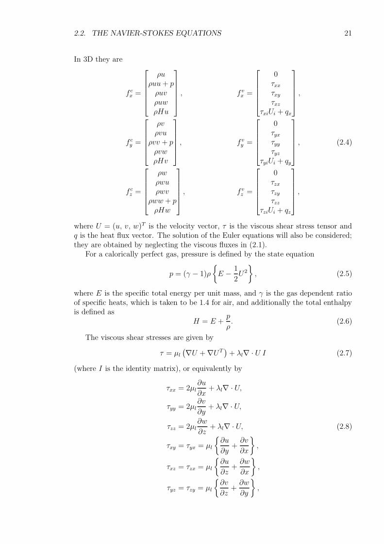
In 3D they are
f cx =
ρuρuu+ pρuvρuwρHu
, f vx =
0τxxτxyτxz
τxiUi + qx
,
f cy =
ρvρvu
ρvv + pρvwρHv
, f vy =
0τyxτyyτyz
τyiUi + qy
, (2.4)
f cz =
ρwρwuρwv
ρww + pρHw
, f vz =
0τzxτzyτzz
τziUi + qz
,
where U = (u, v, w)T is the velocity vector, τ is the viscous shear stress tensor andq is the heat flux vector. The solution of the Euler equations will also be considered;they are obtained by neglecting the viscous fluxes in (2.1).
For a calorically perfect gas, pressure is defined by the state equation
p = (γ − 1)ρ
E − 1
2U2
, (2.5)
where E is the specific total energy per unit mass, and γ is the gas dependent ratioof specific heats, which is taken to be 1.4 for air, and additionally the total enthalpyis defined as
H = E +p
ρ. (2.6)
The viscous shear stresses are given by
τ = µl(∇U +∇UT
)+ λl∇ · U I (2.7)
(where I is the identity matrix), or equivalently by
τxx = 2µl∂u
∂x+ λl∇ · U,
τyy = 2µl∂v
∂y+ λl∇ · U,
τzz = 2µl∂w
∂z+ λl∇ · U, (2.8)
τxy = τyx = µl
∂u
∂y+∂v
∂x
,
τxz = τzx = µl
∂u
∂z+∂w
∂x
,
τyz = τzy = µl
∂v
∂z+∂w
∂y
,
22 CHAPTER 2. DISCRETIZATION AND JACOBIANS
where local laminar bulk viscosity by Stokes hypothesis for a monatomic gas is
λl = −2
3µl. (2.9)
The heat fluxes are given by Fourier’s law,
q = κl∇T, (2.10)
with the thermal conductivity and the temperature defined by
κl =cpµlPrl
, T =p
ρ< , (2.11)
where < is the universal gas constant, which is set to unity when non-dimensionalizingthe equations. The local variation of molecular viscosity with temperature is modelledby Sutherland’s Law,
µl = µl,∞ ·(T
T∞
)1.5
· T∞ + T
T + T, (2.12)
whereby T = 110.4K is Sutherland’s constant. The law is used to model the localvariation in thermal conductivity in exactly the same way, so that
µlµl,∞
=κlκl,∞
, (2.13)
and the Prandtl number
Prl =cpµl,∞κl,∞
, cp = < γ
γ − 1, (2.14)
is constant everywhere.
2.2.2 The Favre Averaged Equations
In order to respect the influence of turbulence without resolving every turbulent eddy,the flow equations are Favre averaged, i.e. time-averaged with mass weighting. Theinstantaneous flow quantities in (2.2) are substituted for Favre averaged quantitiesplus a time-dependent fluctuation, i.e.
W = W +W ′′, (2.15)
where the mass-average is defined as
W (x) =1
ρlimt′→∞
1
t′
∫ t+t′
t
ρ(x, s)W (x, s) ds, (2.16)
where ρ is the conventional Reynolds averaged density. Thus the procedure rests onthe assumption that the time scale of turbulent motion is much shorter than that ofthe mean motion. By mass-averaging the result, the Favre averaged Navier-Stokesequations are obtained.
2.3. FLOW REGIME 23
The equations are substantially identical to the instantaneous flow equations withinstantaneous replaced by mean quantities, except for the introduction of the turbu-lence correlations
ρU ′′ ⊗ U ′′, ρU ′′ ⊗ U ′′ · U , ρh′′U ′′, τ · U ′′, 1
2ρU ′′(U ′′ · U ′′), (2.17)
which are modelled using some closure approximations. All models under consider-ation here use the Boussinesq eddy viscosity assumption (Boussinesq, 1877), whichstates that the Reynolds stress tensor may be modelled as
−ρU ′′ ⊗ U ′′ = µt
(∇U +∇UT − 2
3∇ · U I
)− 2
3ρk I, (2.18)
for a suitable turbulent viscosity µt and turbulent kinetic energy k defined as
k =1
2
ρU ′′ · U ′′ρ
. (2.19)
Thereupon the momentum equations reduce to the instantaneous equations with amodified effective viscosity µe,
µe = µl + µt, (2.20)
and a modified pressure
p∗ = p− 2
3ρk, (2.21)
and the second correlation in (2.17) results in an extra term in the energy equa-tion. Similarly ρh′′U ′′ is approximated as a heat flux, giving an effective thermalconductivity κe,
κe = κl + κt, (2.22)
which replaces κl in the viscous terms. Typically
κt =cpµtPrt
, (2.23)
and the turbulence Prandtl number Prt is a constant. The last two correlationsof (2.17) may be interpreted as diffusion of k, and are therefore included as an extrak diffusion term in the energy equation. See (Wilcox, 1998) for a more completediscussion.
The purpose of a turbulence model is then to provide a value for µt and possiblyk. One-equation models such as Spalart-Allmaras (Spalart & Allmaras, 1992) consistof a transport equation for some modified eddy-viscosity νt, and terms involving kare typically neglected. Two-equation models such as Wilcox k − ω (Wilcox, 1998)provide transport equations for k and one other quantity, µt is then modelled as somefunction of these.
2.3 Flow Regime
The equations of the previous section display radically different behaviour dependingon the flow regime, therefore it is also necessary to indicate the values of the three
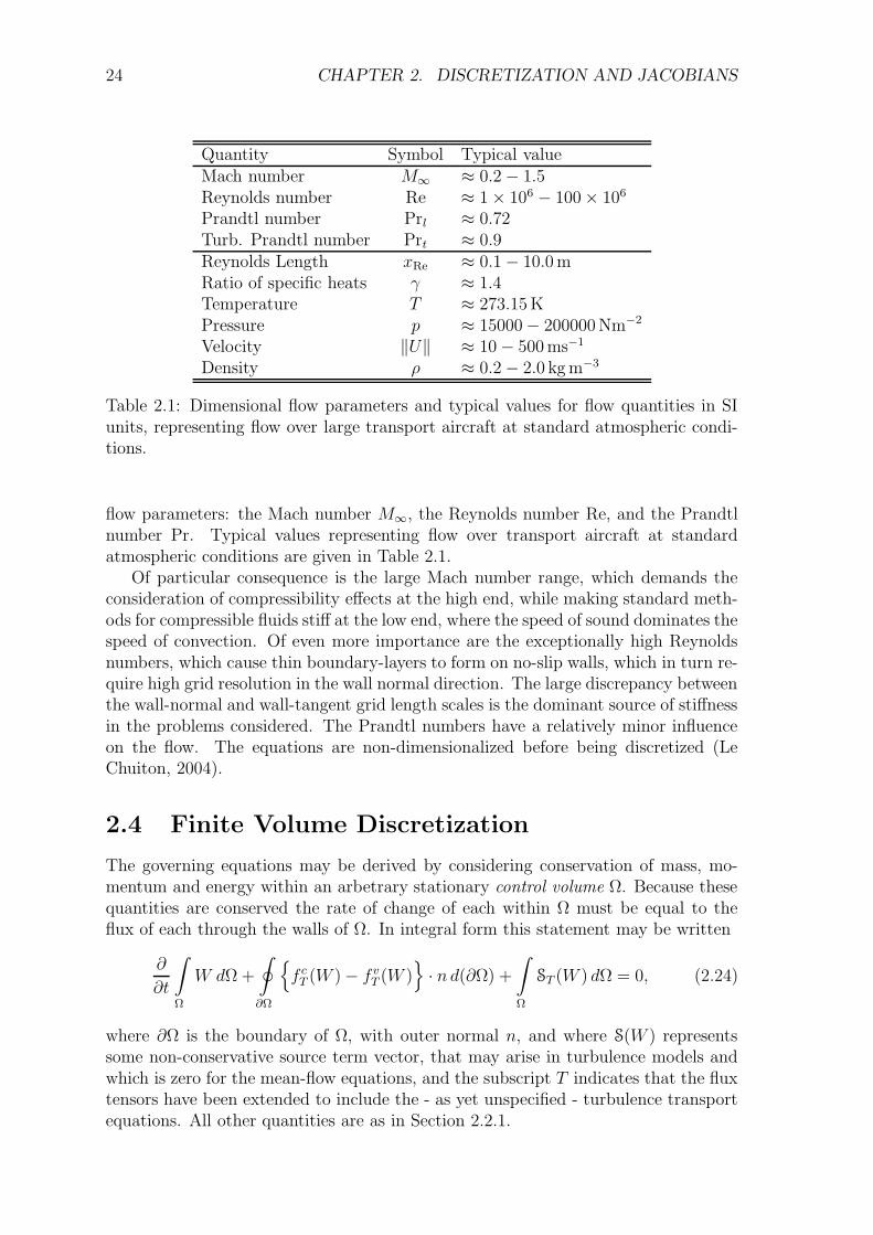
24 CHAPTER 2. DISCRETIZATION AND JACOBIANS
Quantity Symbol Typical valueMach number M∞ ≈ 0.2− 1.5Reynolds number Re ≈ 1× 10⁶ − 100× 106
Prandtl number Prl ≈ 0.72Turb. Prandtl number Prt ≈ 0.9Reynolds Length xRe ≈ 0.1− 10.0 mRatio of specific heats γ ≈ 1.4Temperature T ≈ 273.15 KPressure p ≈ 15000− 200000 Nm−2
Velocity ‖U‖ ≈ 10− 500 ms−1
Density ρ ≈ 0.2− 2.0 kg m−3
Table 2.1: Dimensional flow parameters and typical values for flow quantities in SIunits, representing flow over large transport aircraft at standard atmospheric condi-tions.
flow parameters: the Mach number M∞, the Reynolds number Re, and the Prandtlnumber Pr. Typical values representing flow over transport aircraft at standardatmospheric conditions are given in Table 2.1.
Of particular consequence is the large Mach number range, which demands theconsideration of compressibility effects at the high end, while making standard meth-ods for compressible fluids stiff at the low end, where the speed of sound dominates thespeed of convection. Of even more importance are the exceptionally high Reynoldsnumbers, which cause thin boundary-layers to form on no-slip walls, which in turn re-quire high grid resolution in the wall normal direction. The large discrepancy betweenthe wall-normal and wall-tangent grid length scales is the dominant source of stiffnessin the problems considered. The Prandtl numbers have a relatively minor influenceon the flow. The equations are non-dimensionalized before being discretized (LeChuiton, 2004).
2.4 Finite Volume Discretization
The governing equations may be derived by considering conservation of mass, mo-mentum and energy within an arbetrary stationary control volume Ω. Because thesequantities are conserved the rate of change of each within Ω must be equal to theflux of each through the walls of Ω. In integral form this statement may be written
∂
∂t
∫
Ω
W dΩ +
∮
∂Ω
f cT (W )− f vT (W )
· n d(∂Ω) +
∫
Ω
ST (W ) dΩ = 0, (2.24)
where ∂Ω is the boundary of Ω, with outer normal n, and where S(W ) representssome non-conservative source term vector, that may arise in turbulence models andwhich is zero for the mean-flow equations, and the subscript T indicates that the fluxtensors have been extended to include the - as yet unspecified - turbulence transportequations. All other quantities are as in Section 2.2.1.
2.4. FINITE VOLUME DISCRETIZATION 25
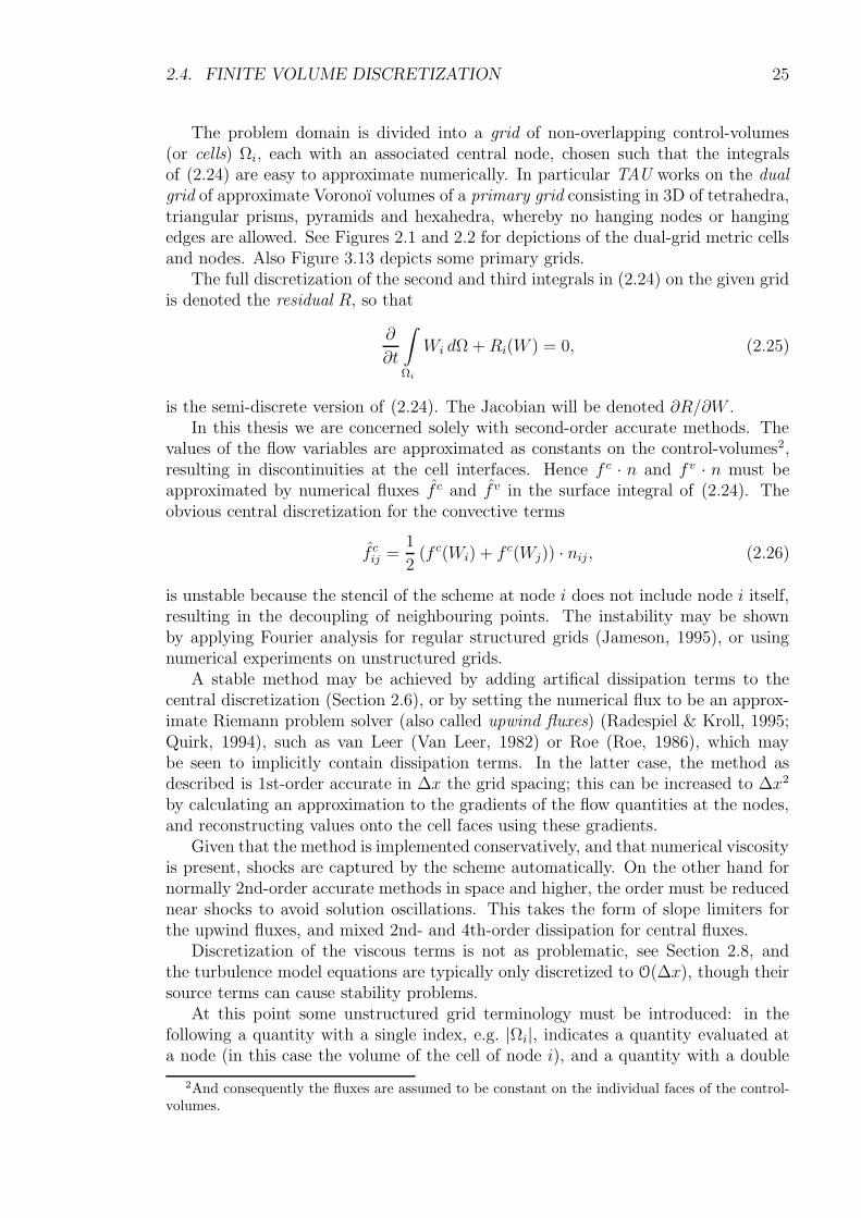
The problem domain is divided into a grid of non-overlapping control-volumes(or cells) Ωi, each with an associated central node, chosen such that the integralsof (2.24) are easy to approximate numerically. In particular TAU works on the dualgrid of approximate Voronoı volumes of a primary grid consisting in 3D of tetrahedra,triangular prisms, pyramids and hexahedra, whereby no hanging nodes or hangingedges are allowed. See Figures 2.1 and 2.2 for depictions of the dual-grid metric cellsand nodes. Also Figure 3.13 depicts some primary grids.
The full discretization of the second and third integrals in (2.24) on the given gridis denoted the residual R, so that
∂
∂t
∫
Ωi
Wi dΩ +Ri(W ) = 0, (2.25)
is the semi-discrete version of (2.24). The Jacobian will be denoted ∂R/∂W .In this thesis we are concerned solely with second-order accurate methods. The
values of the flow variables are approximated as constants on the control-volumes2,resulting in discontinuities at the cell interfaces. Hence f c · n and f v · n must beapproximated by numerical fluxes f c and f v in the surface integral of (2.24). Theobvious central discretization for the convective terms
f cij =1
2(f c(Wi) + f c(Wj)) · nij, (2.26)
is unstable because the stencil of the scheme at node i does not include node i itself,resulting in the decoupling of neighbouring points. The instability may be shownby applying Fourier analysis for regular structured grids (Jameson, 1995), or usingnumerical experiments on unstructured grids.
A stable method may be achieved by adding artifical dissipation terms to thecentral discretization (Section 2.6), or by setting the numerical flux to be an approx-imate Riemann problem solver (also called upwind fluxes) (Radespiel & Kroll, 1995;Quirk, 1994), such as van Leer (Van Leer, 1982) or Roe (Roe, 1986), which maybe seen to implicitly contain dissipation terms. In the latter case, the method asdescribed is 1st-order accurate in ∆x the grid spacing; this can be increased to ∆x2
by calculating an approximation to the gradients of the flow quantities at the nodes,and reconstructing values onto the cell faces using these gradients.
Given that the method is implemented conservatively, and that numerical viscosityis present, shocks are captured by the scheme automatically. On the other hand fornormally 2nd-order accurate methods in space and higher, the order must be reducednear shocks to avoid solution oscillations. This takes the form of slope limiters forthe upwind fluxes, and mixed 2nd- and 4th-order dissipation for central fluxes.
Discretization of the viscous terms is not as problematic, see Section 2.8, andthe turbulence model equations are typically only discretized to O(∆x), though theirsource terms can cause stability problems.
At this point some unstructured grid terminology must be introduced: in thefollowing a quantity with a single index, e.g. |Ωi|, indicates a quantity evaluated ata node (in this case the volume of the cell of node i), and a quantity with a double
2And consequently the fluxes are assumed to be constant on the individual faces of the control-volumes.
26 CHAPTER 2. DISCRETIZATION AND JACOBIANS
index, e.g. nij, indicates a quantity evaluated on the grid face connecting two nodes(in this case the normal vector of said face). The set N(i) of neighbours of i containsindices of all control-volumes that share a face with node i. Similarly B(i) containsindices of all faces of i that lie on the boundary of the computational domain, and isthe empty set if i is not a boundary point. Sometimes it is useful to consider the firstnode that lies normal to the boundary at point i. The set Bnear(i) contains this pointif i is on the boundary, and is otherwise the empty set. The stencil of the discreteresidual R is denoted M.
Henceforth the indices i, j, k, etc. refer to the indices of grid nodes/control-volumes, unless otherwise stated.
2.5 Construction of the Jacobian
In addition to constructing the discrete residual of the scheme R, the Jacobian of thediscrete residual ∂R/∂W is required for implicit methods.
Consider the structure of the Jacobian. R is a vector of size n × N , where n isthe number of nodes in the grid, and N is the number of equations per node. Inprinciple R may be a function of all W , and W is a vector of the same size as R.Then ∂R/∂W is a matrix with dimensions (n×N)× (n×N). The structure of thematrix is dependent on the ordering of the degrees of freedom. It is most convenientto consider orderings of the form
(ρ0, u0, v0, p0, ρ1, u1, · · · , ρn−1, un−1, vn−1, pn−1) ,
in which case the Jacobian may be written as an n×n matrix of N×N blocks. Thenthe notation ∂Ri/∂Wj refers to the block matrix obtained by differentiating the Ncomponents of Ri with respect to the N components of Wj.
However, Ri is not a function of Wj for all j, but only of a small number of Wj
in the vicinity of i. The set of such j corresponds to the stencil of Ri, denoted M(i),which is almost always either (a) only i, (b) i and the immediate neighbours of i, or(c) i and the immediate and next-neighbours of i. Figure 2.1 shows these sets for asimple grid.
If a point j is not in the stencil of Ri then ∂Ri/∂Wj ≡ 0, otherwise it is non-zero.Hence the Jacobian is sparse and the amount of fill-in is determined by the size of M.The Jacobian is typically very large, even accounting for its sparsity, and thereforecomputationally intensive to calculate and store. The problem of efficient handlingof the Jacobian is the main issue in algorithms involving it, and hence forms one ofthe principal themes of this thesis.
To see the importance of stencil size consider Table 2.2 which gives the number ofimmediate neighbours and next-neighbours for several grid types. In three dimensionsthe stencil size increases by at least a factor of four between neighbours and next-neighbours, resulting in a corresponding increase in the fill-in of the Jacobian.
Remark 2.1. It is often the case that we consider the contribution of a flux over aface to the Jacobian. If the flux fij has a stencil of i, j only, then contributions aremade to the Jacobian at four points. Consider the case that the flux modifies R as
Ri := Ri + fij,
Rj := Rj − fij,
2.5. CONSTRUCTION OF THE JACOBIAN 27
Figure 2.1: A stylized example of an unstructured dual-grid resulting from the Voronoıvolumes of a primary grid of equilateral triangles. The nodes of the dual volumes arethe same as the nodes of the primary grid. The shaded control-volumes show possiblestencils of parts of the residual R calculated at the point i. For example the stencilof a 1st-order upwind flux includes i and the immediate neighbours of i, while thestencil of a 2nd-order upwind flux includes additionally the next-neighbours of i, e.g.k.
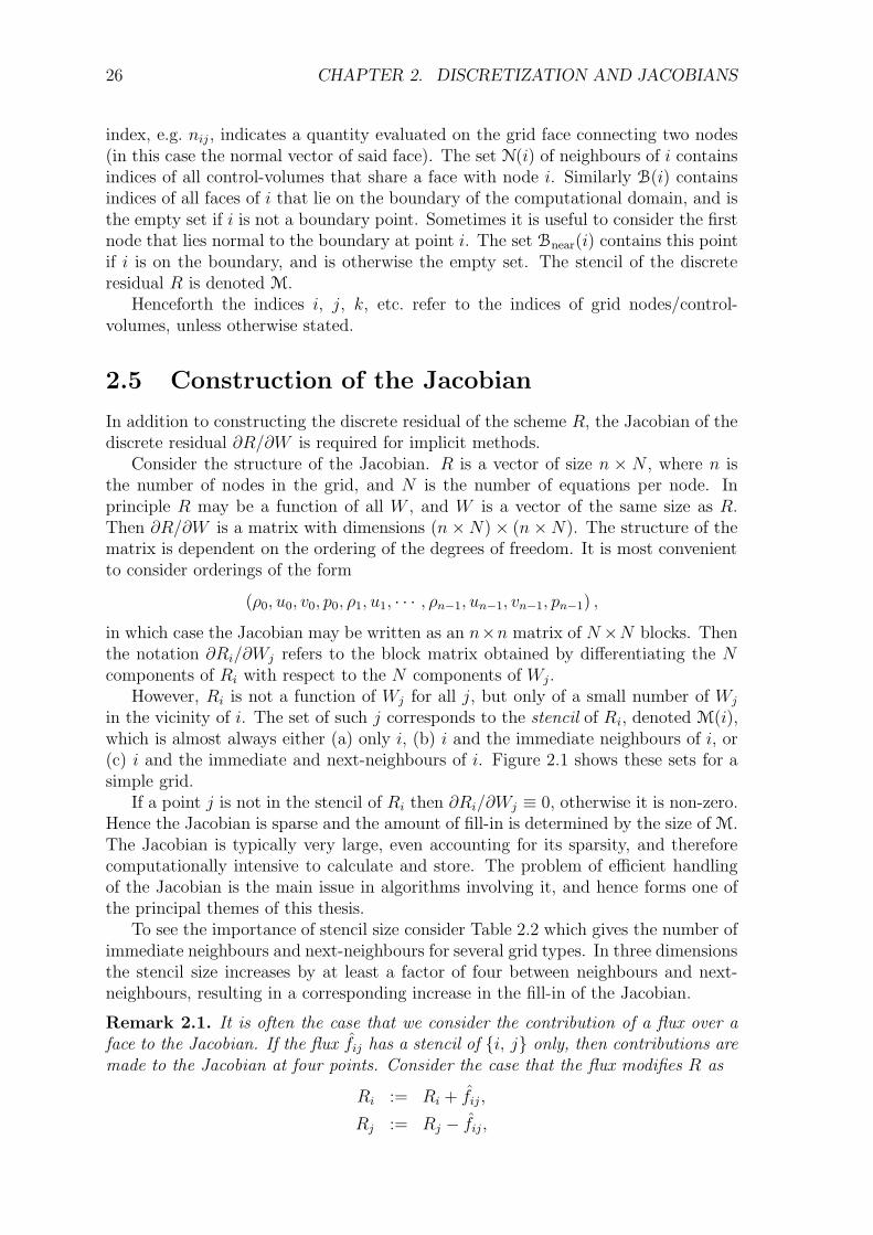
Figure 2.2: As for Figure 2.1, but in the region of a boundary. Important to note isthat some nodes lie directly on the boundary. The values of the flow quantities atthese nodes are taken to represent the state on the boundary (e.g. for a no-slip wall,zero velocity).
28 CHAPTER 2. DISCRETIZATION AND JACOBIANS
Dimensions Grid Type Neighbours Next-neighbours2 Structured 5 132 Unstructured 7 193 Structured 7 333 Semi-Structured 9 353 Unstructured 15 ≈77
Table 2.2: The number of nodes neighbouring any given node on regular 2d and 3dgrids. Here “Structured” indicates a regular square or hexahedral mesh, “Unstruc-tured” a regular triangular or tetrahedral mesh, and “Semi-Structured” a mesh oftriangular prisms. The node counts are inclusive: “Neighbours” includes the pointitself and “Next-neighbours” includes neighbours. The values provide an indicator ofthe relative sizes of Jacobians on the various meshes, with the two stencil sizes.
then it modifies the Jacobian as
∂R
∂W:=
∂R
∂W+
. . .∂fij∂Wi
· · · ∂fij∂Wj
.... . .
...
− ∂fij∂Wi
· · · − ∂fij∂Wj
. . .
. (2.27)
2.6 Central Convective Fluxes
The most commonly used convective flux in TAU is a central flux with blended2nd- and 4th-undivided differences representing 2nd- and 4th-order artificial dissipa-tion, and is an unstructured generalization of the well-known Jameson-Schmitt-Turkel(JST) scheme (Jameson et al., 1981). The term undivided difference simply refers to astandard finite difference approximation to a derivative, but without a denominator;for example the LHS of
Wi+1 − 2Wi +Wi−1 ≈ ∆x2 d2W
dx2.
The 4th-order dissipation is used in the majority of the field as the dissipationterms are of order ∆x3 and therefore do not detract from the order of accuracy ofthe method, which is dominated by the error incurred when approximating the fluxesas constant on faces (∆x2). However the operator is unstable at discontinuities andintroduces overshoots, so 2nd-order dissipation terms of order ∆x are used thereinstead. This reduction of order means it is important to have higher grid resolutionnear shocks than elsewhere. The detection of discontinuities is performed with apressure gradient sensor.
The scheme may be written
f JSTij =
1
2(f c(Wi) + f c(Wj)) · nij −
1
2Dij, (2.28)
where f c are the exact convective fluxes as given in (2.4), and D contains the dissi-pation terms. The derivatives of f c · n are given in various variables in Appendix A.
2.6. CENTRAL CONVECTIVE FLUXES 29
2.6.1 Scalar Dissipation for the Central Scheme
We give the exact form of the dissipation D of (2.28) as implemented in TAU. For acontrol-volume i the total contribution to the residual R is
Di =∑
j∈N(i)
Dij, (2.29)
whereby the dissipation on a face is a sum of 1st- and 3rd-undivided differences
Dij = λcij
[ε
(2)ij (Wj −Wi)− ε(4)
ij (Lj(W )− Li(W ))], (2.30)
and ε(2) and ε(4) control the levels of the two types of dissipation, which themselvesconsist of three terms:
ε(2)ij = ε
(2)ij s
c2ij φij, (2.31)
ε(4)ij = ε
(4)ij s
c4ij φij. (2.32)
The ε(2) and ε(4) act as the shock switch, sc2 and sc4 are intended to make the levelof dissipation independent of the number of neighbours of a cell, and φ is intendedto increase the amount of dissipation across the larger faces of anisotropic cells anddecrease it across the smaller faces. In particular
φij =4φ
(i)ij φ
(j)ji
φ(i)ij + φ
(j)ji + ε
, (2.33)
where ε = 10−16 is a constant chosen simply to prevent a divide-by-zero condition inthe arithmetic. The φ
(i)ij are defined by
φ(i)ij =
(max0
(12λti − λcij
)
2λcij
) 12
, (2.34)
where max0(·) = max(·, 0) and λti is the sum of the maximum convective eigenvaluesover all faces of volume i. The maximum convective eigenvalue denotes is definedin (2.45). Given that φ
(i)ij and φ
(j)ji are approximately the same - which is the case in the
absence of rapid changes in cell size - (2.33) reduces to φ ≈ 2φ(i)ij . Then (2.34) causes
the dissipation over the face of a cell with the larger eigenvalue λc to be relativelyincreased, and that with the smaller eigenvalue to be decreased. In particular, inanisotropic boundary-layer cells, the eigenvalue of the long side dominates that of theshort side and so extra dissipation normal to the wall is included.
The expressions chosen in order to attempt to remove dependence on the numberof faces of a control volume are
sc2ij =3(Ni +Nj)
NiNj, (2.35)
sc4ij =9[(1 +Ni)Ni + (1 +Nj)Nj
]
(1 +Ni)Ni(1 +Nj)Nj, (2.36)
30 CHAPTER 2. DISCRETIZATION AND JACOBIANS
where Ni is the number of faces of cell i,
Ni =∑
j∈N(i)
(1) +∑
b∈B(i)
(1). (2.37)
The coefficients ε(2) and ε(4) are more familiar, being taken directly from Jame-son (Jameson et al., 1981),
ε(2)ij = k(2) max(Ψi,Ψj), (2.38)
ε(4)ij = max0(k(4) − ε(2)
ij ), (2.39)
where k(2) and k(4) are constants allowing specification of absolute levels of dissipation,typically 1/2 and 1/64 respectively, and the remaining terms control the relative levelsof 2nd- and 4th-dissipation using the estimate of the pressure gradient
Ψi =
∣∣∣∣pdifi
pΣi
∣∣∣∣ , (2.40)
where
pΣi =
∑
j∈N(i)
(pi + pj) +∑
m∈Bnear(i)
(3pi − pm), (2.41)
pdifi =
∑
j∈N(i)
(pj − pi) +∑
m∈Bnear(i)
(pi − pm), (2.42)
so that for a smooth solution Ψ and so ε(2) are of order ∆x2, while at a shock bothare of order unity.
The 3rd-difference is constructed as a difference of two 2nd-undivided differences,
Li(W ) =∑
j∈N(i)
(Wj −Wi) +∑
m∈Bnear(i)
(Wi −Wm), (2.43)
where the use of the boundary near points here is intended to avoid asymmetry ofthe Laplacian on boundaries. The total maximum eigenvalue for a cell is
λti =∑
j∈N(i)
λcij +∑
b∈B(i)
λcb, (2.44)
whereby the maximum eigenvalues on the faces are
λcij = maxm
[λm
(∂f cij∂W
)]= 1
2|(Ui + Uj) · nij|+ 1
2(ai + aj)‖nij‖, (2.45)
λcb = maxm
[λm
(∂f cb∂Wb
)]= |Ub · nb|+ ab‖nb‖, (2.46)
where λm(·) returns the mth eigenvalue of the matrix argument, thus completing thescheme.
2.6. CENTRAL CONVECTIVE FLUXES 31
Remark 2.2. This scheme is derived from the JST method (Jameson et al., 1981)which has proven extremely effective on structured grids. The chief difficulty in theextension to unstructured grids is the unidirectional nature of the coefficients of thedissipation in the original scheme. For example the pressure sensor given by Jamesonto construct the shock switch is unidirectional,
ΨIJ =|pI+1,J − 2pI,J + pI−1,J ||pI+1,J + 2pI,J + pI−1,J |
, (2.47)
and repeated in each coordinate direction; here I and J are the structured grid cellindices. Equation (2.40) is an attempt to model this expression without direction in-formation. Similarly (2.33) is an attempt to reproduce the commonly used structuredgrid anisotropic cell scaling
φI+ 12,J,K = 1 + max
(λcI,J+ 1
2,K
λcI+ 1
2,J,K
,λcI,J,K+ 1
2
λcI+ 1
2,J,K
) 12
, (2.48)
in three dimensions, where e.g. λcI+ 1
2,J,K
is the average of the eigenvalues of the faces of
cell I, J,K with face normals pointing in the I direction. The coefficients sc2 and sc4
have no equivalent in the structured scheme and are chosen such that the unstructuredscheme on a regular hexahedral dual grid has the same level of dissipation as thestructured scheme on a regular structured grid.
2.6.2 Jacobian of Dissipation under a Constant Coefficient
Approximation
As seen in Section 2.6.1 the full dissipation operator is rather complex, and the exactderivatives thereof are therefore also very complex. By assuming that the derivativesof the coefficients of the difference operators in the scheme - namely ε(2), ε(4) and λc
- may be treated as constants with respect to W , a considerable simplification in theJacobian is achieved.
Remark 2.3. We attempt to justify this approximation: consider the relative magni-tudes of the terms that are neglected in the derivative, and the remaining terms. Forconcise presentation consider only the second difference operator without the shockswitch,
D2ndij = λcij(Wj −Wi). (2.49)
The full derivative of this may then be written
∂λcij∂Wk
(Wj −Wi) + λcij∂
∂Wk
(Wj −Wi), (2.50)
however, under the assumption λc = const., only the second term appears. Considerthe magnitude of these quantities in terms of ∆x the grid spacing.
If k /∈ i, j then all derivatives in (2.50) are zero, so consider the case k ∈ i, j.For a smooth solution (Wj −Wi) is of order ∆x, whereas its derivative is of orderunity. Also λcij and its derivate are always order ∆x (due to the presence of the facenormal n). Therefore the first term in (2.50) has order ∆x2 and the second term
32 CHAPTER 2. DISCRETIZATION AND JACOBIANS
order ∆x. Hence the first term may be neglected for smooth solutions on sufficientlyfine grids, and the approximation λc = const. is justified.
Extending this argument to the full dissipation operator, is complicated by the dif-ferences present in pdif, whose derivatives are also of order unity, but a similar resultis eventually achieved. Experiences using the approximate Jacobian in Chapter 5 bearout the conclusions given here.
The derivatives may then be written
∂Di
∂Wk=
∑
j∈N(i)
∂Dij
∂Wk(2.51)
=∑
j∈N(i)
λcij
[ε
(2)ij
∂
∂Wk(Wj −Wi)− ε(4)
ij
∂
∂Wk(Lj(W )− Li(W ))
], (2.52)
whereby choosing the conservative variables for the differentiation pays off in a par-ticularly simple form for the difference derivatives:
∂
∂Wk(Wj −Wi) =
−I k = i
I k = j
0 otherwise
, (2.53)
where I is the identity matrix, so that the derivative of their sum is
∂
∂Wk
∑
j∈N(i)
(Wj −Wi) =
∑j∈N(i)(−I) k = i
I k ∈ N(i)
0 otherwise
. (2.54)
The pseudo-Laplacian derivatives are similarly
∂Li(W )
∂Wk
=
∑j∈N(i)(−I) +
∑m∈Bnear(i)(I) k = i
I k ∈ N(i) ∩ Bnear(i)
0 otherwise
, (2.55)
and the expression for the Jacobian is complete.Comparing this result with the exact Jacobian given in Section 2.6.3 highlights
the enormous potential benefits of well-chosen approximations.
2.6.3 Full Jacobian of Scalar Dissipation
The full expression for the exact Jacobian of the scalar dissipation operator is givenin the following. Note that extensive use is made of the chain rule to divide theoperation into manageable parts. Each expression of Section 2.6.1 is differentiatedin turn, writing the derivative in terms of derivatives of the other quantities. Noattempt is made to collect terms in an effort to reduce the number of expressions.This helps reduce the likelihood of an error and allows the scheme derivative to beeasily verified against the scheme statement.
2.6. CENTRAL CONVECTIVE FLUXES 33
Starting with the dissipation contribution to the residual at a node,
∂Di
∂Wk
=∑
j∈N(i)
∂Dij
∂Wk
(2.56)
=∑
j∈N(i)
∂λcij∂Wk
[ε
(2)ij (Wj −Wi)− ε(4)(Lj − Li)
]
+ λcij
[∂ε
(2)ij
∂Wk(Wj −Wi) + ε
(2)ij
∂
∂Wk(Wk −Wi) (2.57)
−∂ε
(4)ij
∂Wk(Lj − Li)− ε(4)
ij
∂
∂Wk(Lj − Li)
];
comparing with (2.52) the extra effort required is already apparent. The individualfluxes are then
∂ε(2)ij
∂Wk= sc2ij
(∂ε
(2)ij
∂Wkφij + ε
(2)ij
∂φij∂Wk
), (2.58)
∂ε(4)ij
∂Wk= sc4ij
(∂ε
(4)ij
∂Wkφij + ε
(4)ij
∂φij∂Wk
), (2.59)
whereby
∂φij∂Wk
=
4
[(∂φ
(i)ij
∂Wkφ
(j)ji + φ
(i)ij
∂φ(j)ji
∂Wk
)(φ
(i)ij + φ
(j)ji + ε)− φ(i)
ij φ(j)ji
(∂φ
(i)ij
∂Wk+
∂φ(j)ji
∂Wk
)]
(φ(i)ij + φ
(j)ji + ε)2
. (2.60)
Note that the ε used to prevent a divide-by-zero condition in the arithmetic of theflux, prevents this condition in the derivative as well.
The appearance of max(·, ·) in the expression for φ(i)ij (and similarly, the appear-
ance of | · | in the expression for Ψ), leads to the derivative of φ(i)ij being undefined at
(12λti − λcij). This problem will be discussed further later; for the moment differenti-
ate the function correctly where possible, and choose the limit from one side for thederivative at the discontinuity:
∂φ(i)ij
∂Wk=
∂∂Wk
( 12λti−λcij2λcij
) 12 1
2λti − λcij ≥ 0
0 12λti − λcij < 0
. (2.61)
Experience shows that such effects are not harmful to the linearization. Continuingthe derivation
∂
∂Wk
(12λti − λcij2λcij
) 12
=
(12
∂λti∂Wk− ∂λcij
∂Wk
)2λcij −
(12λti − λcij
)2∂λcij∂Wk
(λcij)2
· 1
2
(12λti − λcij2λcij
)− 12
, (2.62)
34 CHAPTER 2. DISCRETIZATION AND JACOBIANS
and the shock switch introduces another discontinuity,
∂ε(2)ij
∂Wk= k(2) ∂
∂Wk
[max(Ψi,Ψj)
]=
k(2) ∂Ψi
∂WkΨi > Ψj
k(2) ∂Ψj∂Wk
Ψi ≤ Ψj
, (2.63)
∂ε(4)ij
∂Wk=
∂
∂Wk
[max0(k(4) − ε(2)
ij )]
=
−∂ε
(2)ij
∂Wkk(4) − ε(2)
ij > 0
0 otherwise, (2.64)
and again,
∂Ψi
∂Wk=
∂
∂Wk
∣∣∣∣pdifi
pΣi
∣∣∣∣ =
∂∂Wk
(pdifi
pΣi
)pdifi
pΣi≥ 0
− ∂∂Wk
(pdifi
pΣi
)pdifi
pΣi< 0
, (2.65)
whereby
∂
∂Wk
(pdifi
pΣi
)=
∂pdifi
∂WkpΣi + pdif
i∂pΣi
∂Wk
(pΣi )2
. (2.66)
The derivatives of the pressure differences are comparatively straightforward,
∂pΣi
∂Wk=
∑j∈N(i)(
∂pi∂Wi
) +∑
m∈Bnear(i) 3 ∂pi∂Wi
k = i∂pk∂Wk
k ∈ N(i) ∩ Bnear(i)
0 otherwise
, (2.67)
∂pdifi
∂Wk
=
∑j∈N(i)(− ∂pi
∂Wi) +
∑m∈Bnear(i)
∂pi∂Wi
k = i∂pk∂Wk
k ∈ N(i) ∩Bnear(i)
0 otherwise
, (2.68)
and can be further simplified by performing the differentiation in primitive variables.The pseudo-Laplacians are exactly as in Section 2.6.2
∂Li(W )
∂Wk=
∑j∈N(i)(−I) +
∑m∈Bnear(i)(I) k = i
I k ∈ N(i) ∩ Bnear(i)
0 otherwise
, (2.69)
and finally the derivatives of the maximum eigenvalues on the faces are
∂λcij∂Wk
=
12∂∂Wk
[(Ui + Uj) · nij + (ai + aj)‖nij‖] (Ui + Uj) · nij ≥ 0,12∂∂Wk
[−(Ui + Uj) · nij + (ai + aj)‖nij‖] (Ui + Uj) · nij < 0,, (2.70)
whereby
∂
∂Wk
[12(Ui + Uj) · nij + 1
2(ai + aj)‖nij‖
]=
12
∂Ui·nij∂Wi
+ 12∂ai∂Wi‖nij‖ k = i
12
∂Uj ·nij∂Wj
+ 12
∂aj∂Wj‖nij‖ k = j
0 otherwise
,
∂
∂Wk
[−1
2(Ui + Uj) · nij + 1
2(ai + aj)‖nij‖
]=
similarly,
completing the expression for the Jacobian.
2.7. GRADIENT APPROXIMATION 35
2.7 Gradient Approximation
In the construction of the viscous fluxes and turbulence source terms, the gradientsof the flow quantities in space are needed. These may be obtained by a least-squaresmethod, i.e. fitting a plane to a local collection of nodes, but a particularly elegantand efficient gradient on a general grid is obtained with the Gauss integral theo-rem (Blazek, 2001). Consider the identity
∫
Ωi
∇Wi dΩ =
∮
∂Ωi
Wi n · d(∂Ω), (2.71)
whereby approximating these integrals numerically gives
Ωi∇WGGi :=
∑
j∈N(i)
1
2(Wi +Wj)nij +
∑
m∈B(i)
Wi nm, (2.72)
where including the integral over boundary faces ensures that the approximate sur-face integral is closed. This procedure is known as the Green-Gauss method for thegradient.
2.7.1 Green-Gauss Jacobian
Another advantage of Green-Gauss gradients is that their derivatives are particularlysimple. In particular
Ωi∂
∂Wk
∇WGGi =
∑j∈N(i)
12nij +
∑m∈B(i) nm k = i
12nik k ∈ N(i)
0 otherwise
. (2.73)
Here it is also apparent that the stencil of the gradient consists of immediate neigh-bours only.
2.8 Viscous Flux Modelling
The modelling of viscous fluxes is not as critical as that of the convective fluxes, asthere are no related stability problems. The exact expressions for the viscous fluxesare used to model the fluxes on cell faces, and therefore all that is required are thevalues of the flow variables and their gradients on the face. The flow variables arealways averaged from the two neighbouring cells,
Uij :=1
2(Ui + Uj) , (2.74)
but there are several approaches to obtain the gradient on the face.Most simply the average of the gradients in the neighbouring cells are taken,
∇Uij :=1
2(∇Ui +∇Uj) , (2.75)
36 CHAPTER 2. DISCRETIZATION AND JACOBIANS
where ∇U is approximated by Green-Gauss, Section 2.7. On the other hand it seemsclear that the most accurate and stable approximation to the gradient normal to theface is the difference
(∇Uij · nij) ≈Uj − Ui‖xj − xi‖
, (2.76)
where xi is the coordinate of node i, so that a better full gradient approximationmight be
∇Uij =Uj − Ui‖xj − xi‖
∆x +∇Uij −
(∇Uij · ∆x
)∆x, (2.77)
where ∆x = (xj − xi)/‖xj − xi‖.Both these expressions for the gradient have the disadvantage of having stencils
consisting of all immediate neighbours of both i and j - leading to a next-neighbourfill-in in the viscous Jacobian. On the other hand by neglecting completely face-tangential gradient components we have
∇UTSLij ≈ Uj − Ui
‖xj − xi‖, (2.78)
which also has a simple expressions for its derivatives. Viscous fluxes based on thisgradient will be denoted the Thin Shear-Layer (TSL) fluxes, due to their similarityto a method in structured codes in which only viscous fluxes normal to the wall areconsidered. Here, however, fluxes in all directions are considered.
It may be shown that the use of the TSL gradient results in a consistent vis-cous flux discretization, and numerical tests show that the influence on the solutionis very minor, even for cases sensitive to viscous effects such as high-lift configura-tions. Further, it is used in some unstructured codes, on the basis that it improvesrobustness (Mavriplis, 1998).
2.8.1 TSL Viscous Flux Derivatives
The numerical viscous fluxes for a given face in conservative variables are
f vij =
0nlτlxnlτlynlτlz
nl(τlmUm + ql)
,
where τ and q are given in Section 2.2.1. If TSL gradients are used, derivatives of µand κ are neglected, and if further the differentiation is performed with respect to thealternative primitive variables, Appendix A.2, then the Jacobian takes a particularlysimple form. With respect to the alternative primitive variables at nodes i and j
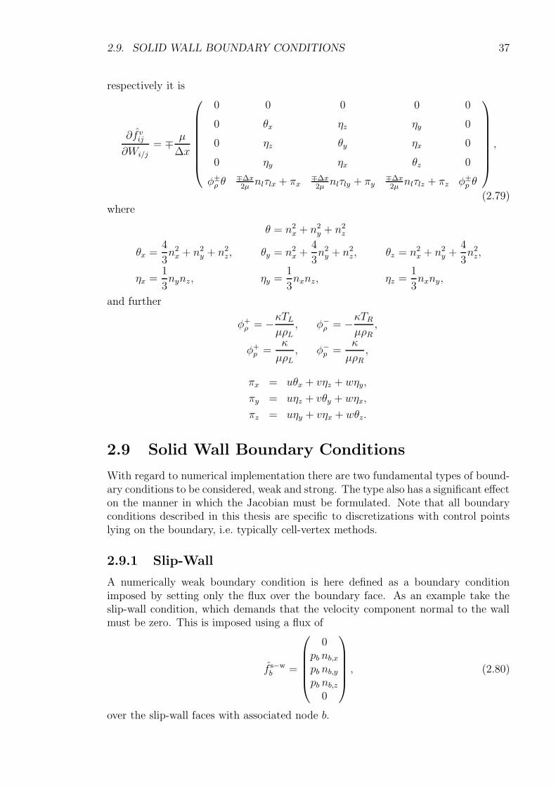
2.9. SOLID WALL BOUNDARY CONDITIONS 37
respectively it is
∂f vij∂Wi/j
= ∓ µ
∆x
0 0 0 0 0
0 θx ηz ηy 0
0 ηz θy ηx 0
0 ηy ηx θz 0
φ±ρ θ∓∆x2µnlτlx + πx
∓∆x2µ
nlτly + πy∓∆x2µ
nlτlz + πz φ±p θ
,
(2.79)where
θ = n2x + n2
y + n2z
θx =4
3n2x + n2
y + n2z, θy = n2
x +4
3n2y + n2
z, θz = n2x + n2
y +4
3n2z,
ηx =1
3nynz, ηy =
1
3nxnz, ηz =
1
3nxny,
and further
φ+ρ = −κTL
µρL, φ−ρ = −κTR
µρR,
φ+p =
κ
µρL, φ−p =
κ
µρR,
πx = uθx + vηz + wηy,
πy = uηz + vθy + wηx,
πz = uηy + vηx + wθz.
2.9 Solid Wall Boundary Conditions
With regard to numerical implementation there are two fundamental types of bound-ary conditions to be considered, weak and strong. The type also has a significant effecton the manner in which the Jacobian must be formulated. Note that all boundaryconditions described in this thesis are specific to discretizations with control pointslying on the boundary, i.e. typically cell-vertex methods.
2.9.1 Slip-Wall
A numerically weak boundary condition is here defined as a boundary conditionimposed by setting only the flux over the boundary face. As an example take theslip-wall condition, which demands that the velocity component normal to the wallmust be zero. This is imposed using a flux of
f s−wb =
0pb nb,xpb nb,ypb nb,z
0
, (2.80)
over the slip-wall faces with associated node b.
38 CHAPTER 2. DISCRETIZATION AND JACOBIANS
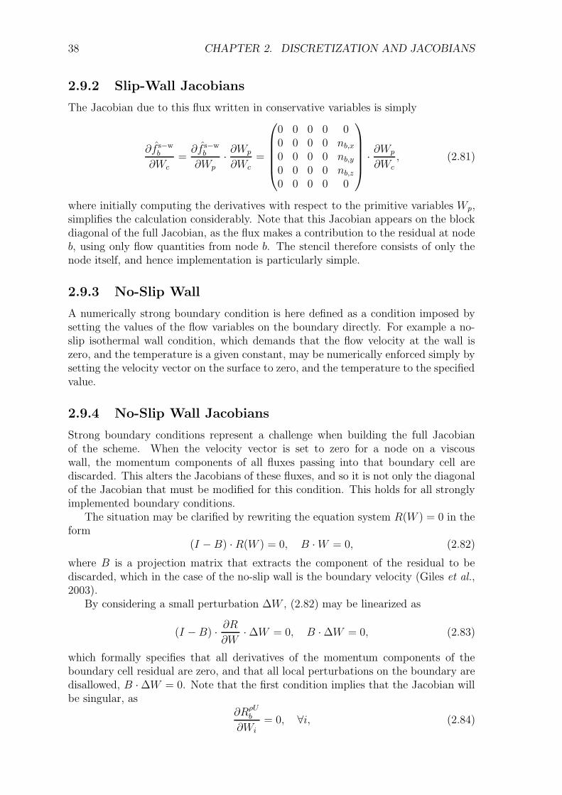
2.9.2 Slip-Wall Jacobians
The Jacobian due to this flux written in conservative variables is simply
∂f s−wb
∂Wc=∂f s−w
b
∂Wp· ∂Wp
∂Wc=
0 0 0 0 00 0 0 0 nb,x0 0 0 0 nb,y0 0 0 0 nb,z0 0 0 0 0
· ∂Wp
∂Wc, (2.81)
where initially computing the derivatives with respect to the primitive variables Wp,simplifies the calculation considerably. Note that this Jacobian appears on the blockdiagonal of the full Jacobian, as the flux makes a contribution to the residual at nodeb, using only flow quantities from node b. The stencil therefore consists of only thenode itself, and hence implementation is particularly simple.
2.9.3 No-Slip Wall
A numerically strong boundary condition is here defined as a condition imposed bysetting the values of the flow variables on the boundary directly. For example a no-slip isothermal wall condition, which demands that the flow velocity at the wall iszero, and the temperature is a given constant, may be numerically enforced simply bysetting the velocity vector on the surface to zero, and the temperature to the specifiedvalue.
2.9.4 No-Slip Wall Jacobians
Strong boundary conditions represent a challenge when building the full Jacobianof the scheme. When the velocity vector is set to zero for a node on a viscouswall, the momentum components of all fluxes passing into that boundary cell arediscarded. This alters the Jacobians of these fluxes, and so it is not only the diagonalof the Jacobian that must be modified for this condition. This holds for all stronglyimplemented boundary conditions.
The situation may be clarified by rewriting the equation system R(W ) = 0 in theform
(I −B) ·R(W ) = 0, B ·W = 0, (2.82)
where B is a projection matrix that extracts the component of the residual to bediscarded, which in the case of the no-slip wall is the boundary velocity (Giles et al.,2003).
By considering a small perturbation ∆W , (2.82) may be linearized as
(I −B) · ∂R∂W·∆W = 0, B ·∆W = 0, (2.83)
which formally specifies that all derivatives of the momentum components of theboundary cell residual are zero, and that all local perturbations on the boundary aredisallowed, B ·∆W = 0. Note that the first condition implies that the Jacobian willbe singular, as
∂RρUb
∂Wi= 0, ∀i, (2.84)
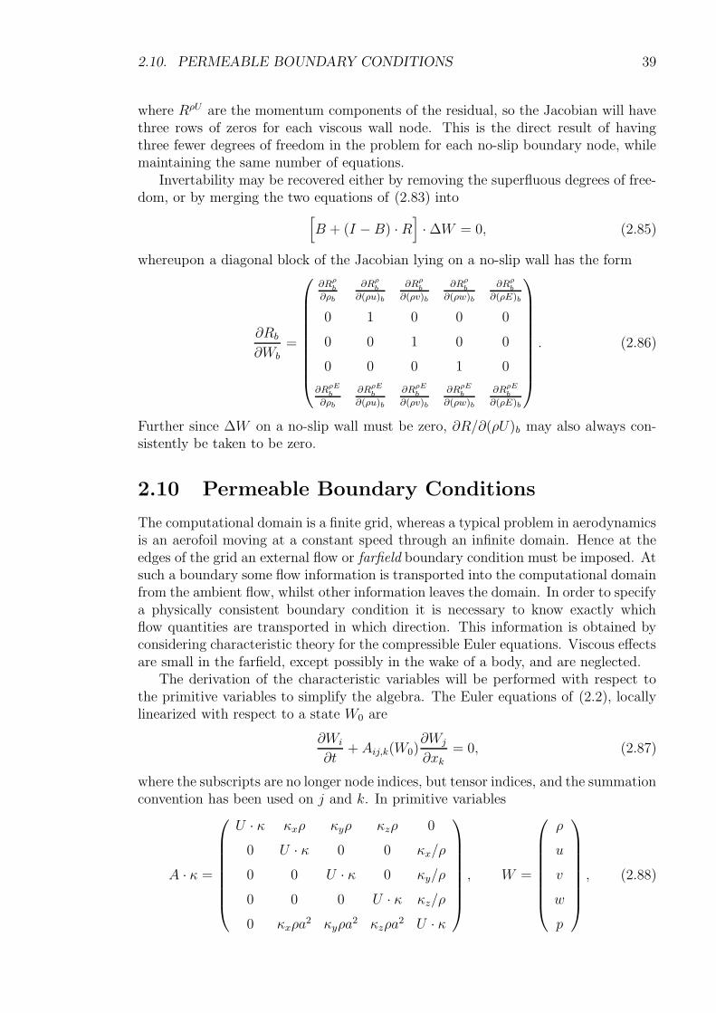
2.10. PERMEABLE BOUNDARY CONDITIONS 39
where RρU are the momentum components of the residual, so the Jacobian will havethree rows of zeros for each viscous wall node. This is the direct result of havingthree fewer degrees of freedom in the problem for each no-slip boundary node, whilemaintaining the same number of equations.
Invertability may be recovered either by removing the superfluous degrees of free-dom, or by merging the two equations of (2.83) into
[B + (I −B) ·R
]·∆W = 0, (2.85)
whereupon a diagonal block of the Jacobian lying on a no-slip wall has the form
∂Rb
∂Wb=
∂Rρb∂ρb
∂Rρb∂(ρu)b
∂Rρb∂(ρv)b
∂Rρb∂(ρw)b
∂Rρb∂(ρE)b
0 1 0 0 0
0 0 1 0 0
0 0 0 1 0
∂RρEb∂ρb
∂RρEb∂(ρu)b
∂RρEb∂(ρv)b
∂RρEb∂(ρw)b
∂RρEb∂(ρE)b
. (2.86)
Further since ∆W on a no-slip wall must be zero, ∂R/∂(ρU)b may also always con-sistently be taken to be zero.
2.10 Permeable Boundary Conditions
The computational domain is a finite grid, whereas a typical problem in aerodynamicsis an aerofoil moving at a constant speed through an infinite domain. Hence at theedges of the grid an external flow or farfield boundary condition must be imposed. Atsuch a boundary some flow information is transported into the computational domainfrom the ambient flow, whilst other information leaves the domain. In order to specifya physically consistent boundary condition it is necessary to know exactly whichflow quantities are transported in which direction. This information is obtained byconsidering characteristic theory for the compressible Euler equations. Viscous effectsare small in the farfield, except possibly in the wake of a body, and are neglected.
The derivation of the characteristic variables will be performed with respect tothe primitive variables to simplify the algebra. The Euler equations of (2.2), locallylinearized with respect to a state W0 are
∂Wi
∂t+ Aij,k(W0)
∂Wj
∂xk= 0, (2.87)
where the subscripts are no longer node indices, but tensor indices, and the summationconvention has been used on j and k. In primitive variables
A · κ =
U · κ κxρ κyρ κzρ 0
0 U · κ 0 0 κx/ρ
0 0 U · κ 0 κy/ρ
0 0 0 U · κ κz/ρ
0 κxρa2 κyρa
2 κzρa2 U · κ
, W =
ρ
u
v
w
p
, (2.88)
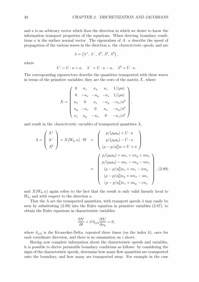
40 CHAPTER 2. DISCRETIZATION AND JACOBIANS
and κ is an arbitrary vector which fixes the direction in which we desire to know theinformation transport properties of the equations. When deriving boundary condi-tions κ is the surface normal vector. The eigenvalues of A · κ describe the speed ofpropagation of the various waves in the direction κ, the characteristic speeds, and are
λ =(λ+, λ−, λ0, λ0, λ0
),
whereλ+ = U · κ+ a, λ− = U · κ− a, λ0 = U · κ.
The corresponding eigenvectors describe the quantities transported with these wavesin terms of the primitive variables; they are the rows of the matrix X, where
X =
0 κx κy κz 1/(ρa)
0 −κx −κy −κz 1/(ρa)
κx 0 κz −κy −κx/a2
κy −κz 0 κx −κy/a2
κz κy −κx 0 −κz/a2
,
and result in the characteristic variables of transported quantities Λ,
Λ =
Λ+
Λ−
Λ0
= X(W0, κ) ·W =
p/(ρ0a0) + U · κp/(ρ0a0)− U · κ
(ρ− p/a20)κ+ U × κ
=
p/(ρ0a0) + uκx + vκy + wκz
p/(ρ0a0)− uκx − vκy − wκz(ρ− p/a2
0)κx + vκz − wκy(ρ− p/a2
0)κy + wκx − uκz(ρ− p/a2
0)κz + uκy − vκx
, (2.89)
and X(W0, κ) again refers to the fact that the result is only valid linearly local toW0, and with respect to the direction κ.
That the Λ are the transported quantities, with transport speeds λ may easily beseen by substituting (2.89) into the Euler equation in primitive variables (2.87), toobtain the Euler equations in characteristic variables:
∂Λi
∂t+ λiδij,k
∂Λj
∂xk= 0,
where δij,k is the Kronecker-Delta, repeated three times (on the index k), once foreach coordinate direction, and there is no summation on i above.
Having now complete information about the characteristic speeds and variables,it is possible to derive permeable boundary conditions as follows: by considering thesigns of the characteristic speeds, determine how many flow quantities are transportedonto the boundary, and how many are transported away. For example in the case
2.10. PERMEABLE BOUNDARY CONDITIONS 41
of subsonic flow out of the domain λ+ and λ0 are positive while λ− is negative,implying that Λ+ and Λ0 are transported onto the boundary from the field, and Λ−
is determined at the boundary. Hence one may choose a single flow variable to be seton the boundary termed the physical boundary condition; in general one must choosea set of variables corresponding to the number of negative eigenvalues3.
Having chosen a variable, or set of variables to specify on the boundary, theremaining flow quantities are found as solutions of the numerical boundary conditions.Since the characteristic variables are transported directly onto the boundary, we musthave
Λib(Wc) = Λi
e(Wc)
for all those Λi for which λi is positive. Here b signifies a point on the boundary, ande an imaginary point immediately outside the domain near b. The linearization inthe computation of the characteristic variables is performed with respect to the stateat b.
In TAU the farfield boundary condition is implemented as follows: for each bound-ary point λ are found, and so the condition type determined, subsonic or supersonic,inflow or outflow. For subsonic outflow the pressure at e is specified as the physicalcondition, for subsonic inflow pressure and velocity at e are specified. The boundaryis then regarded as a Riemann problem and solved as such for the flux through theassociated boundary face, resulting in a weak boundary condition. The approximateRiemann solver used bears no relation to that used for the interior fluxes.
The derivation of the numerical boundary condition for the subsonic outflow caseis given as an example in the following section.
2.10.1 Subsonic Outflow Condition
Consider the case of specifying the pressure pBC on a subsonic outflow surface,whereby κ is chosen to be the surface normal vector n. From the previous section theconditions at the boundary are
pb = pBC - one physical condition
Λ+b (Wb) = Λ+
e (Wb) - one numerical condition
Λ0b(Wb) = Λ0
e(Wb) - three numerical conditions
and so the numerical conditions expanded read
(Ue · n) + pe/(ρbab) = Λ+b (Wb),
(ρe − pe/a2b)n+ Ue × n = Λ0
b(Wb).
By substituting pBC for pe in both equations, and taking the dot product of thesecond equation with n, a simple expression for ρe is obtained. An expression for Uethen follows directly giving:
We =
ρe
Ue
pe
=
Λ0b · n+ pBC/a
2b(
Λ+b − pBC/(ρbab)
)n+ n× Λ0
b
pBC
, (2.90)
3The choice of variables to set is not completely free however; it is obviously not possible to setΛ+ on a subsonic outflow boundary for example. See (Hirsch, 1989) for a complete discussion.
42 CHAPTER 2. DISCRETIZATION AND JACOBIANS
whereby it has been noted that the tangential velocity component Ut satisfies
Ut = n× Λ0 = n× (U × n) = U − (U · n)n.
Equation (2.90) may be simplified further by substituting in the expressions for Λb,and is the desired boundary condition.
2.11 Turbulence Model Discretization
Two classes of turbulence models are used in this thesis: one-equation models typifiedby Spalart-Allmaras (SA) (Spalart & Allmaras, 1992), introduce a transport equationfor a quantity closely related to the turbulence eddy viscosity, denoted νt. Two-equation models introduce transport equations for the turbulent kinetic energy k andone other quantity, typified by the Wilcox k − ω model.
In both cases the transport equations are given by
∂(ρφ)
∂t+∇ · (ρUφ− µte∇φ)− S, (2.91)
where ρφ is the transported quantity, convected with the flow, µte is a turbulenceeffective viscosity, and S is a source term acting as a volume contribution to theresidual rather than a conservative flux.
The source terms in all models considered here are discretized such that the sourceterm at node i requires flow quantities and gradients at node i only, i.e. they havea stencil of immediate neighbours. Thus use of only 1st-order accurate convectivefluxes together with the choice of TSL gradients in the diffusion terms, means thatthe stencil of the entire turbulence model discretization may consist only of immediateneighbours. This reduces the fill-in of the Jacobian, and hence allows the effectiveuse of implicit methods for the turbulence equations.
In this section the SA and closely related Spalart-Allmaras-Edwards (SAE) (Ed-wards & Chandra, 1996) models are fully described as they are implemented in TAU.
2.11.1 Expression for the Eddy-Viscosity
Given the SA/SAE transported quantity νt at a given point, there is an explicitalgebraic expression for the eddy-viscosity νt, there:
νt =χ3
χ3 + c3v1
ρmax(νt, 0), (2.92)
χ =νtνl, (2.93)
where cv1 is a turbulence model constant taken as 7.1.
2.11.2 Convective Fluxes
In TAU the convective terms occurring in all turbulence models are discretized usingthe same fully upwinded scheme with piecewise constant face reconstruction (re-gardless of the discretization of the mean-flow convection), having therefore order of
2.11. TURBULENCE MODEL DISCRETIZATION 43
accuracy ∆x in space. If the turbulent transported quantity is (ρφ) then the fluxfunction may be written
f c,tij = 12qij(ρiφi + ρjφj)− 1
2|qij|(ρjφj − ρiφi), (2.94)
whereqij = 1
2(Ui + Uj) · nij, (2.95)
so that if qij > 0, (2.94) is independent of Wj and vice versa.
2.11.3 Diffusion Fluxes
Similarly to the convective fluxes, all turbulence model transport equations share adiffusive flux discretization. Again using ρφ for the transported quantity,
f v,tij = µte∇φ · n (2.96)
≈ µteφj − φi‖∆x‖ , (2.97)
i.e. TSL gradients, where the effective turbulent viscosity µte is different from theeffective viscosity of the mean-flow equations µe, and is defined differently for one-and two-equation models. For SA/SAE it is simply
µte =µl + µttσm
, (2.98)
µl = 12(µl,i + µl,j), (2.99)
µtt = 12(ρiνt,i + ρj νt,j) (2.100)
where σm = 23
is a model constant.
2.11.4 Spalart-Allmaras Source Terms
The Spalart-Allmaras source term at a given node (indices dropped for simplicity) is
SSA = P −D + d,
P = cb1 · ρνt ·(|ω|+ fv2 ·
ρνtρκ2d2
wall
),
D = cw1 ·(ρνt)
2
ρd2wall
· fw,
d =cb2σm
ρ‖∇νt‖2,
where P , D and d are production, destruction and diffusion terms respectively, dwallis the distance to the nearest wall, and
fv2 = 1− χ
1 + χ · fv1, fv1 =
χ3
χ3 + c3v1
, χ =µtµl
=ρνtµl,
fw = g · g1/6lim, g = r + cw2 ·
(r6 − r
), r =
rsω + fv2 · rs
,
rs =ρνt
ρκ2d2wall
, glim =1 + c6
w3
g6 + c6w3
,
44 CHAPTER 2. DISCRETIZATION AND JACOBIANS
where ω is the vorticity,
ω2 =
(∂u
∂y− ∂v
∂x
)2
+
(∂v
∂z− ∂w
∂y
)2
+
(∂w
∂x− ∂u
∂z
)2
, (2.101)
κ = 0.4100 is the Karman constant, and all quantities remaining undefined are othermodel constants. In particular
cb1 = 0.1355, cb2 = 0.6220, cv1 = 7.1000,
cw1 =cb1κ2
+1 + cb2σm
, cw2 = 0.3000, cw3 = 2.0000,
σm = 0.6667.
2.11.5 Spalart-Allmaras-Edwards Source Terms
The only difference between the SA and SAE models lies in the source term. TheSAE source term for a single node is
SSAE = P −D + d,
P = cb1 · ρνt · frot · sfac · σ,D = cw1ρνt · rs · fw,d =
cb2σm
ρ‖∇νt‖2,
where once again P , D and d are production, destruction and diffusion terms respec-tively, dwall is the distance to the nearest wall, and
σ =√
max(vσ, 0), sfac = fv1 +1
max(χ, ε)
and frot ≡ 1 if no rotation correction is used. In addition
vσ = 2
[(∂u
∂x
)2
+
(∂v
∂y
)2
+
(∂w
∂z
)2]
+
(∂u
∂y+∂v
∂x
)2
+
(∂u
∂z+∂w
∂x
)2
+
(∂w
∂y+∂v
∂z
)2
− 2
3
(∂u
∂x+∂v
∂y+∂w
∂z
)2
,
and
s = max(sfac · σ, ε) fv1 =χ3
χ3 + c3v1
, χ =µtµl
=ρνtµl,
fw = g · g1/6lim, g = r + cw2 ·
(r6 − r
), r =
tanh(rs/s)
tanh(1),
rs =ρνt
ρκ2d2wall
, glim =1 + c6
w3
g6 + c6w3
,
where ε = 10−16 prevents a divide by zero condition, and where all remaining unde-fined quantities are model constants, taking values identical to those given in Sec-tion 2.11.4.
2.12. SUMMARY 45
2.11.6 Boundary Conditions
Farfield boundary conditions are trivial, as there is only one convective speed in theturbulence equations, the flow speed, and no production or destruction. For fullyturbulent calculations some fraction of the laminar viscosity at the farfield is takenfor νt,∞, i.e.
νt,∞ = σ∞νl,
where σ∞ is some turbulence model constant. On viscous walls νt is set to zero,corresponding to the absence of turbulent eddies very near to the wall.
2.12 Summary
A complete finite volume scheme on unstructured grid has been described for theFavre averaged Navier-Stokes equations, including a description of certain one-equationturbulence models. In parallel with the description of the discretization, the deriva-tives of the terms involved have been calculated and described, insofar as this is pos-sible in limited space. For those terms of the discretization for which a particularlycompact Jacobian exists, or for which through a suitable simplicifaction a compactJacobian can be produced, the Jacobians have been given and the simplification jus-tified. In particular, an original argument has been given for a common simplificationof the derivatives of the JST scheme (that of the assumption of constant coefficients).No justification for this approximation has been seen previously in the literature bythe author.
The solution of the discretized equations presented in this chapter is consideredin the remainder of the thesis. The Jacobians developed are used as part of animplicit method, whereby the complexity of these Jacobians, demonstrated here inSection 2.6.3, limits the extent to which the exact derivatives can be applied. On theother hand the exact Jacobians without approximation will be seen to be useful inother contexts, in particular in aerodynamic design, Chapter 5.
Chapter 3
Approximately Factored ImplicitSchemes
3.1 Introduction
An implicit method for convergence acceleration for stationary solutions of the RANSequations is developed based on the requirements that (i) the memory usage shouldnot significantly exceed that of Runge-Kutta, (ii) implementation should be relativelyeasy, (iii) parallelization should be possible and efficient, (iv) the method should beat least as robust as RK. A method satisfying these conditions would then be a slot-in substitute for Runge-Kutta in any application. If in addition it achieves betterconvergence performance in terms of CPU time, then the performance of the solverwill have been improved with no drawbacks.
The method developed in this chapter is a novel variant of the Lower-Upper Sym-metric Gauss-Seidel (LU-SGS) scheme, which has its origins in CFD in (Jameson &Turkel, 1981), which considers a Newton method with a very lax Jacobian approx-imation, resulting in a linear system that is inexactly solved using a single step ofa symmetric Gauss-Seidel method. The name LU-SGS implies in particular the useof a first-order Jacobian, introduced in (Yoon & Jameson, 1986a), and the use ofthe resulting scheme as a FAS multigrid smoother (Yoon & Jameson, 1986b; Yoon& Jameson, 1988). The novel aspects of the scheme presented here are described inSection 1.1.2.
The body of this chapter is divided into three sections. Section 3.2 contains a fulldescription of the modifed LU-SGS scheme as it applies to finite volume discretiza-tions of the RANS equations on unstructured grids, including details such as implicithandling of dual-time iterations. Section 3.3 contains a detailed theoretical analysisof the scheme; principally an assessment of the stability of the Gauss-Seidel itera-tion by means of a generalized theory of diagonal dominance, Fourier analysis, and ademonstration of the time-accuracy of the scheme. Section 3.4 is then concerned withnumerical results, the cornerstones of which are an investigation of the effects of thevarious approximations made in Section 3.2, parallel performance results, and finallya comparison of the relative efficiencies of LU-SGS and Runge-Kutta as multigridsmoothers for large engineering test cases. In the following “Runge-Kutta” refers tothe explicit Runge-Kutta method with residual smoothing, local time stepping andFAS multigrid, as described in (Jameson & Baker, 1984).
46
3.2. DESCRIPTION OF THE SCHEME 47
3.2 Description of the Scheme
Starting with the governing equations in a semi-discrete form, from (2.25):
∂
∂t
∫
Ωi
Wi dΩ +Ri(W ) = 0, (3.1)
and assuming that the node i is at the baricenter of the control volume Ωi, and furtherthat W varies linearly within Ω, we have
|Ωi|dWi
dt+Ri(W ) = 0, (3.2)
where |Ωi| is the volume of Ωi. The system is further discretized in time. A somewhatgeneral three-level discretization may be written
|Ωni |Mn
i
∆tn∆W n
i = − β
1 + αRn+1i − 1− β
1 + αRni +
α
1 + α
|Ωn−1i |Mn−1
i
∆tn−1∆W n−1
i , (3.3)
Here ∆W n = W n+1−W n, Rn = R(W n), and M is the mass matrix. The superscriptsdenote the time level, with all quantities up to and including time level n known, andW n+1 unknown. Since only the steady state solution is of interest, the mass matrixis lumped: M = I, and we set α = 0, which eliminates dependence on the solutionat time tn−1, giving
|Ωni |
∆tn∆W n
i = −βRn+1i − (1− β)Rn
i . (3.4)
Equation (3.4) is a non-linear algebraic system for ∆W n, which may be solved by ap-plication of Newton’s method as follows. The system is linearized about the solutionat time tn, so that
Ri(Wn+1) = Ri(W
n) +∂Ri(W
n)
∂t∆tni + O(∆t2),
= Ri(Wn) +
∑
j∈M(i)
∂Ri(Wn)
∂Wj
∂W nj
∂t∆tni + O(∆t2), (3.5)
where the time step ∆t may vary within the grid such that the CFL number isconstant, and where M(i) is the set of grid points in the stencil of Ri, emphasisingthat contributions from ∂Ri/∂Wj where j 6∈ M(i) are zero. Substituting (3.5) into(3.4), and applying
∂W nj
∂t∆tn = ∆W n
j + O(∆t2), (3.6)
results in the linear algebraic system
|Ωi|∆ti
δij + β∂Ri(W
n)
∂Wj
·∆W n
j = −Ri(Wn), (3.7)
A(W n) ·∆W n = −R(W n), (3.8)
where A represents the implicit system matrix. Equation (3.8) encapsulates theimplicit scheme: the right-hand side (RHS) of this equation is known as the RHS of
48 CHAPTER 3. APPROXIMATELY FACTORED IMPLICIT SCHEMES
the scheme and contains all elements of the spatial discretization. However if W is theexact solution of the discrete system, then R(W ) ≡ 0 and therefore by (3.8), ∆W = 0independently of A, provided only that it is non-singular. Hence the left-hand side(LHS), of (3.8) has no effect on the converged solution, and may be freely chosen toimprove convergence.
The method for solving the steady state system R(W ) = 0 might then proceed asfollows:
• Linearize (3.4) about W n; in particular evaluate A(W n) to form (3.8).
• Solve (3.8) to obtain ∆W n and hence W n+1.
• Repeat until ∆W n < εtol or ‖R(W n)‖ < εtol.
For 1/∆t = 0 and β = 1 the method reduces to Newton’s method which hasthe properties of quadratic convergence for W 0 in the domain of approximate zeros ofR (Butcher, 1987). In practice the region of W 0 for which the method converges tendsnot to contain the typical initial condition, which is taken as constant flow values,everywhere conforming to the farfield condition (while other boundary conditions areviolated), which is possible as time accuracy is not required. Thus some distinctstart-up technique is required.
This chapter considers only methods which use approximate Jacobians (known asapproximate Newton methods), inexact linear system solvers (inexact Newton meth-ods), and finite values of ∆t. Such methods tend not to have the undesirable proper-ties of Newton methods, and in addition are much easier to formulate, as the Jacobianneed not be calculated exactly. Further the additional flexibility in the constructionof such methods allows the avoidance of many problems traditionally associated withimplicit schemes, namely large memory requirements, high computational cost periteration, and difficulty of parallelization.
There are two critical choices to be made when defining an implicit method, theapproximation to the Jacobian, and the method for solution of the resulting linearsystem. These choices cannot be made independently, as discussed in Section 1.1, itmaking little sense to solve a very approximate system to extremely high accuracy,and just as little to spend a great deal of effort building an exact Jacobian, and thenincurring a large error by solving very approximately. Since it is the aim of this chap-ter to develop a method of very low memory requirements, and it is expected thatmany approximations to the Jacobian must be made in order to achieve this goal,only low-powered linear solvers are candidates. There are only two main possibilities,Jacobi and Gauss-Seidel, with the option perhaps to use a line solver in structuredregions of the grid. Symmetric Gauss-Seidel has the advantage of achieving commu-nication between every pair of nodes in the grid, within one iteration, and is thereforethe starting point. This method is described in the next section, followed by detailsof the approximate Jacobian.
3.2.1 Symmetric Gauss-Seidel (SGS) Solution
The Gauss-Seidel method may be written as follows: given a non-singular linearsystem A · x = b, decompose the system matrix A into a purely lower triangular part
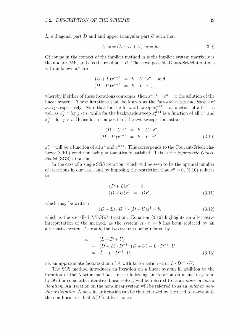
3.2. DESCRIPTION OF THE SCHEME 49
L, a diagonal part D and and upper triangular part U such that
A · x = (L +D + U) · x = b. (3.9)
Of course in the context of the implicit method A is the implicit system matrix, x isthe update ∆W , and b is the residual −R. Then two possible Gauss-Seidel iterationswith unknown xn are
(D + L)xn+1 = b− U · xn, and
(D + U)xn+1 = b− L · xn,
whereby if either of these iterations converges, then xn+1 = xn = x the solution of thelinear system. These iterations shall be known as the forward sweep and backwardsweep respectively. Note that for the forward sweep xn+1
i is a function of all xn aswell as xn+1
j for j < i, while for the backwards sweep xn+1i is a function of all xn and
xn+1j for j > i. Hence for a composite of the two sweeps, for instance
(D + L)x∗ = b− U · xn,(D + U)xn+1 = b− L · x∗, (3.10)
xn+1i will be a function of all xn and xn+1. This corresponds to the Courant-Friedrichs-
Lewy (CFL) condition being automatically satisfied. This is the Symmetric Gauss-Seidel (SGS) iteration.
In the case of a single SGS iteration, which will be seen to be the optimal numberof iterations in our case, and by imposing the restriction that x0 = 0, (3.10) reducesto
(D + L)x∗ = b,
(D + U)x1 = Dx∗, (3.11)
which may be written(D + L) ·D−1 · (D + U)x1 = b, (3.12)
which is the so-called LU-SGS iteration. Equation (3.12) highlights an alternativeinterpretation of the method, as the system A · x = b has been replaced by analternative system A · x = b, the two systems being related by
A = (L+D + U)
= (D + L) ·D−1 · (D + U)− L ·D−1 · U= A− L ·D−1 · U, (3.13)
i.e. an approximate factorization of A with factorization error L ·D−1 · U .The SGS method introduces an iteration on a linear system in addition to the
iteration of the Newton method. In the following an iteration on a linear system,by SGS or some other iterative linear solver, will be referred to as an inner or lineariteration. An iteration on the non-linear system will be referred to as an outer or non-linear iteration. A non-linear iteration can be characterized by the need to re-evaluatethe non-linear residual R(W ) at least once.
50 CHAPTER 3. APPROXIMATELY FACTORED IMPLICIT SCHEMES
For the purposes of comparison, the Jacobi method for solution of the linearsystem is also examined in Section 3.4, written
Dxn+1 = b− (U + L) · xn, (3.14)
whereby Jacobi(n) will refer to a scheme with n Jacobi iterations per non-linear step.In constrast to SGS, two nodes in the grid with a shortest connecting path of m gridedges, will only communicate with each other after m Jacobi iterations. Hence theCFL condition is limited by m times the local cell dimension.
3.2.2 Inviscid Flux Jacobians
Next the construction of the Jacobian of the method is described. Consider theinviscid flux balance on an control volume using a numerical flux f , and a numericalboundary flux fb. Let the values on the left and right sides of the face WL, WR beapproximated by piecewise constant reconstruction of the cell values, so thatWL = Wi
and WR = Wj, then
Ri =∑
j∈N(i)
f(WL,WR;nij) +∑
m∈B(i)
fb(WL;nm)
=∑
j∈N(i)
f(Wi,Wj;nij) +∑
m∈B(i)
fb(Wi;nm), (3.15)
where as before N(i) is the set of all immediate neighbours of point i in the grid, andB(i) is the set of all neighbouring boundary faces. Assuming that f may be writtenin dissipation form
f(WL,WR;nij) =1
2(f c(WL) + f c(WR)) · nij −
1
2D(WL,WR;nij), (3.16)
where f c is the exact convective flux tensor given in (2.4), and further noting thatthe central part of this flux consists of terms of the form of the product f c · n, allowsrewriting (3.15) as
Ri =1
2f c(Wi) ·
∑
j∈N(i)
nij +1
2
∑
j∈N(i)
f c(Wj) · nij
− 1
2
∑
j∈N(i)
D(Wi,Wj;nij) +∑
m∈B(i)
fb(Wi;nm). (3.17)
For a closed control volume i, not touching any boundaries∑
j∈N(i)
nij = 0, (3.18)
and thus for such a control volume the dependence of Ri on Wi occurs only over thedissipation D. Differentiating Ri with respect to Wi results in the diagonal of theJacobian matrix, which for a non-boundary control volume is now just
∂Ri
∂Wi
=1
2
∑
j∈N(i)
∂D(Wi,Wj;nij)
∂Wi
. (3.19)
3.2. DESCRIPTION OF THE SCHEME 51
Thus choosing a flux function with a particularly simple dissipation component deriva-tive, results in a particularly simple Jacobian matrix diagonal. For example takingthe first order Lax-Friedrichs numerical flux
fLF (WL,WR;n) =1
2(F (WL;n) + F (WR;n))
− 1
2|α| (WR −WL), (3.20)
|α| =
∣∣∣∣ρ(∂F
∂W
)∣∣∣∣= |U · n|+ ‖n‖a, (3.21)
and treating α as constant with respect to W when differentiating, gives the Jacobianof the convective residual
∂DLF (Wi,Wj;nij)
∂Wi=
1
2|α|I. (3.22)
So that the derivative of the dissipation, and by (3.19) the diagonal of the Jacobianmatrix, is a positive scalar multiple of the identity matrix.
In contrast off-diagonal blocks of the Jacobian matrix are in general dense, andare constructed exactly for the Lax-Friedrichs scheme as
∂Ri
∂Wj=
1
2
∂f cj∂Wj
− 1
2|α|I, (3.23)
where the convective flux-Jacobian ∂f/∂W is given explicitly in Appendix A.Note that for the LU-SGS method, the only part of the Jacobian that must be
stored and inverted directly is the block diagonal, see (3.11). Thus the propertydescribed by (3.22) is very desirable: firstly it implies that rather than having tostore an N × N matrix at each grid point, it is only necessary to store a scalar,reducing the memory cost by 25 times for the Euler equations. Secondly the cost ofinverting the diagonal is reduced from that of an N ×N matrix inversion to a singledivision.
Of course these savings are only preserved if all other components of the LHSdiscretization (fb, viscous fluxes, turbulence fluxes and sources, etc.), have Jacobianswhose diagonal blocks are also diagonal. This will be discussed in the followingsections.
3.2.3 Viscous Flux Jacobians
The construction of the viscous Jacobian proceeds in the same manner as that of theinviscid. First the operator is simplified such that the stencil of Ri contains only theimmediate neighbours of the point i. In the case of the viscous fluxes this is doneby replacing the full, Green-Gauss gradient based flux by the TSL approximation ofSection 2.8.
The off-diagonal entries of the Jacobian may be taken directly from the formu-lae given in Section 2.8.1, but the Jacobian block diagonal is not diagonal itself,damaging the simplicity and memory requirements of LU-SGS. This is corrected by
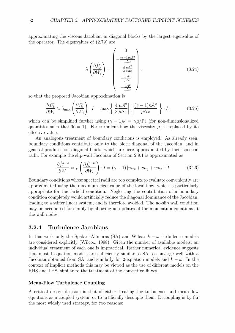
52 CHAPTER 3. APPROXIMATELY FACTORED IMPLICIT SCHEMES
approximating the viscous Jacobian in diagonal blocks by the largest eigenvalue ofthe operator. The eigenvalues of (2.79) are
λ
(∂f vij∂Wi
)=
0
− (γ−1)κA2
ρ∆x
−43µA2
ρ∆x
−µA2
ρ∆x
−µA2
ρ∆x
, (3.24)
so that the proposed Jacobian approximation is
∂f vij∂Wi
≈ λmax
(∂f vij∂Wi
)· I = max
∣∣∣∣4
3
µA2
ρ∆x
∣∣∣∣ ,∣∣∣∣(γ − 1)κA2
ρ∆x
∣∣∣∣· I, (3.25)
which can be simplified further using (γ − 1)κ = γµ/Pr (for non-dimensionalizedquantities such that < = 1). For turbulent flow the viscosity µ, is replaced by itseffective value.
An analogous treatment of boundary conditions is employed. As already seen,boundary conditions contribute only to the block diagonal of the Jacobian, and ingeneral produce non-diagonal blocks which are here approximated by their spectralradii. For example the slip-wall Jacobian of Section 2.9.1 is approximated as
∂f s−wb
∂Wc≈ ρ
(∂f s−wb
∂Wc
)· I = (γ − 1) |unx + vny + wnz| · I. (3.26)
Boundary conditions whose spectral radii are too complex to evaluate conveniently areapproximated using the maximum eigenvalue of the local flow, which is particularlyappropriate for the farfield condition. Neglecting the contribution of a boundarycondition completely would artificially reduce the diagonal dominance of the Jacobian,leading to a stiffer linear system, and is therefore avoided. The no-slip wall conditionmay be accounted for simply by allowing no updates of the momentum equations atthe wall nodes.
3.2.4 Turbulence Jacobians
In this work only the Spalart-Allmaras (SA) and Wilcox k − ω turbulence modelsare considered explicitly (Wilcox, 1998). Given the number of available models, anindividual treatment of each one is impractical. Rather numerical evidence suggeststhat most 1-equation models are sufficiently similar to SA to converge well with aJacobian obtained from SA, and similarly for 2-equation models and k − ω. In thecontext of implicit methods this may be viewed as the use of different models on theRHS and LHS, similar to the treatment of the convective fluxes.
Mean-Flow Turbulence Coupling
A critical design decision is that of either treating the turbulence and mean-flowequations as a coupled system, or to artificially decouple them. Decoupling is by farthe most widely used strategy, for two reasons:
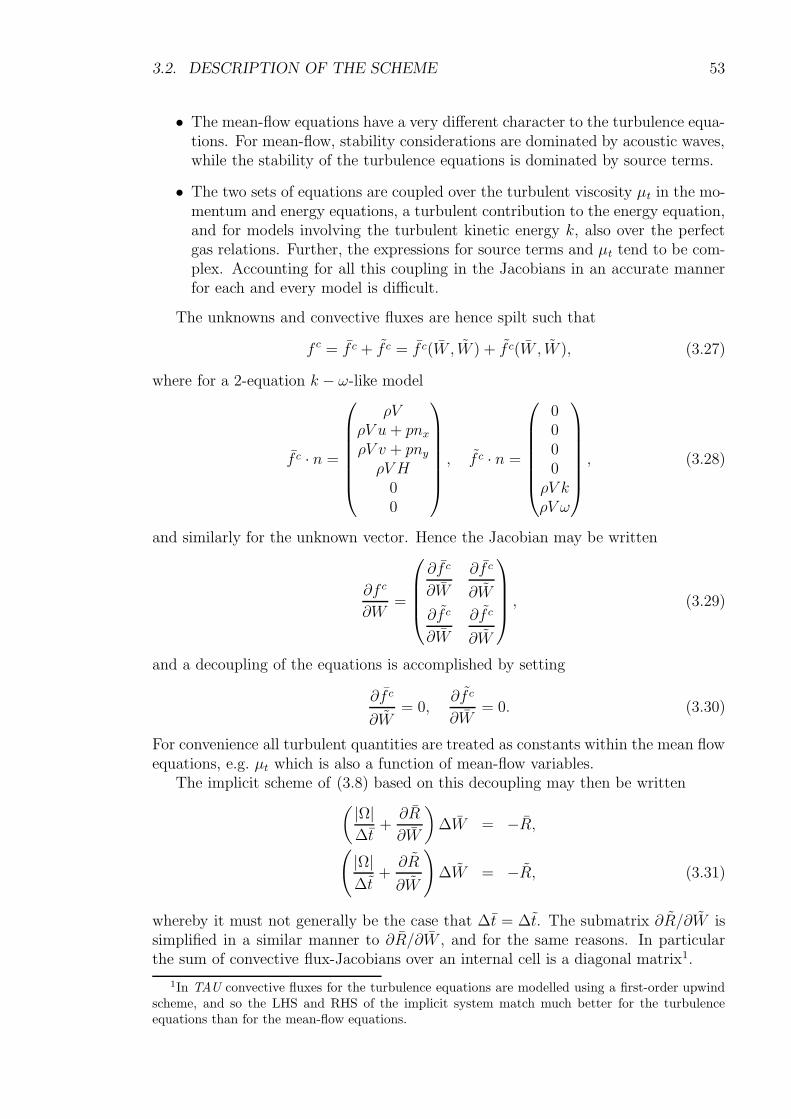
3.2. DESCRIPTION OF THE SCHEME 53
• The mean-flow equations have a very different character to the turbulence equa-tions. For mean-flow, stability considerations are dominated by acoustic waves,while the stability of the turbulence equations is dominated by source terms.
• The two sets of equations are coupled over the turbulent viscosity µt in the mo-mentum and energy equations, a turbulent contribution to the energy equation,and for models involving the turbulent kinetic energy k, also over the perfectgas relations. Further, the expressions for source terms and µt tend to be com-plex. Accounting for all this coupling in the Jacobians in an accurate mannerfor each and every model is difficult.
The unknowns and convective fluxes are hence spilt such that
f c = f c + f c = f c(W , W ) + f c(W , W ), (3.27)
where for a 2-equation k − ω-like model
f c · n =
ρVρV u+ pnxρV v + pnyρV H
00
, f c · n =
0000
ρV kρV ω
, (3.28)
and similarly for the unknown vector. Hence the Jacobian may be written
∂f c
∂W=
∂f c
∂W
∂f c
∂W
∂f c
∂W
∂f c
∂W
, (3.29)
and a decoupling of the equations is accomplished by setting
∂f c
∂W= 0,
∂f c
∂W= 0. (3.30)
For convenience all turbulent quantities are treated as constants within the mean flowequations, e.g. µt which is also a function of mean-flow variables.
The implicit scheme of (3.8) based on this decoupling may then be written( |Ω|
∆t+∂R
∂W
)∆W = −R,
(|Ω|∆t
+∂R
∂W
)∆W = −R, (3.31)
whereby it must not generally be the case that ∆t = ∆t. The submatrix ∂R/∂W issimplified in a similar manner to ∂R/∂W , and for the same reasons. In particularthe sum of convective flux-Jacobians over an internal cell is a diagonal matrix1.
1In TAU convective fluxes for the turbulence equations are modelled using a first-order upwindscheme, and so the LHS and RHS of the implicit system match much better for the turbulenceequations than for the mean-flow equations.
54 CHAPTER 3. APPROXIMATELY FACTORED IMPLICIT SCHEMES
On an implementational note: it is not necessary to solve the two systems of(3.31) separately; in fact it is more efficient in terms of operation counts to formulateand solve them simultaneously, as many quantities (e.g. the coefficient of artificialviscosity) appear in the fluxes and Jacobians of both systems.
Turbulence Diffusion Fluxes
Referring to Section 2.11.3 for the definition of the turbulence diffusion fluxes basedon TSL flow gradients, the Jacobian can be seen to be
∂f v,tij∂W[ji]
= ±Aijµte
∆xij, (3.32)
with respect to primitive variables. For 2-equation turbulence models this derivationproceeds independently for each turbulence variable, and hence the resulting 2 × 2matrix is diagonal.
Turbulent wall boundary conditions are treated strongly, therfore the discussionof Section 3.2.3 with regard to the no-slip wall applies. It remains to consider sourceterms.
Source terms for Spalart-Allmaras
The sources of SA contain terms of the form ∂u/∂x. A full differentiation of theseterms with respect to all variables would imply differentiation of the gradient ofU , resulting in off-diagonal terms in the Jacobian. In contrast, differentiation ofthe sources with respect to the turbulent variables alone results in a block diagonalJacobian; hence decoupling the mean-flow and turbulence equations has simplifiedthe scheme dramatically.
Even so, the complexity of the expressions for the source terms encourages furtherapproximations to the Jacobian. In particular the exact differentiation is complicatedby the terms rs and g in Section 2.11.4, so several considerable approximations aremade (e.g. constant χ) to obtain the approximate Jacobians of the production, de-struction and cross-flow terms for LU-SGS:
dP
d(ρνt)≈ cb1
(|ω|+ 2fv2
ρνtρκ2d2
wall
), (3.33)
dD
d(ρνt)≈ 2cw1k
ρνtρκ2d2
wall
fw, (3.34)
dd
d(ρνt)≈ −cb2s
2
ρ(∇νt · ∇ρ). (3.35)
It is common practice in turbulence modelling to ensure that the source term Jacobianis positive thereby avoiding the use of a limiter (Spalart & Allmaras, 1992). Sincethe source term is subtracted from the residual, e.g. in 2.91, only negative terms arekept:
dSSAd(ρνt)
≈ − dD
d(ρνt)+ min
dd
d(ρνt), 0
≤ 0. (3.36)
This treatment has a serious deficiency: it may be the case that the production anddestruction Jacobians are both very large, but almost cancel each other out. But from
3.3. ANALYSIS OF THE SCHEME 55
(3.36) a large contribution will be made to the Jacobian, which may be interpretedas a reduction of the time step. In such a situation very poor convergence will occur.However in this case stability considerations outweigh efficiency considerations.
3.2.5 Dual-Time Treatment
Dual-time is a time-accurate stepping method consisting of solving an implicit timediscretization, such as a backward difference formula (BDF), by writing the solutionat each time step as a steady state problem, and solving this using known, time-inaccurate methods, see (Jameson, 1991).
In this case the time derivative of (3.2) is discretized with a BDF, and the resultingalgebraic system is solved by progressing the equation
∂W ∗
∂τ= −
|Ω|(3W ∗ − 4W n +W n−1)
2∆t+R(W ∗)
= −R∗(W ∗) (3.37)
to a steady state in τ . Here τ is an artificially introduced pseudo time, W ∗ is theiterate, and the iterations are known as inner iterations. At a steady state ∂W ∗/∂τ =0 and hence W ∗ = W n+1. This system strongly resembles the original problem(3.2) for the steady state case, and so LU-SGS may be applied here. Note that themodification to the residual modifies the Jacobian in the scheme as
∂R∗
∂W ∗ =∂R
∂W ∗ +3
2∆t· I, (3.38)
so that the correct treatment of the additional term increases the diagonal dominanceof the system. Numerical experiments show that when using this technique, LU-SGSis more stable than usual.
3.3 Analysis of the Scheme
Though it is easy to quantify the performance of a scheme in practical applications,simply by implementing and testing it, such a procedure offers few insights into whythe scheme behaves as it does, where it is particularly weak, and how it may beimproved. For such insight theoretical results are vital, even involving - as theygenerally do - substantial simplifications.
The convergence of the LU-SGS scheme is first investigated using the theoryof stability of linear fixed-point iterations extended to account for block-structuredmatrices, Section 3.3.1. It is shown that the exact Jacobian of the Euler spatial dis-cretization is not block diagonally dominant (a weaker condition than diagonal domi-nance), nor is the approximate Jacobian of LU-SGS. Thereupon a modified Jacobianis proposed that is only just diagonally dominant, and therefore the SGS iterationis guaranteed to converge. The new scheme (LU-DD) is implemented and it is seennumerically that while the inner SGS iteration converges much better than the orig-inal scheme, the non-linear convergence is much poorer due to the greater mismatchbetween the residual and Jacobian. Hence it is concluded that diagonal-dominance ismuch too strong a condition on the Jacobian, and hence the corresponding stabilityresults are not useful in this context.
56 CHAPTER 3. APPROXIMATELY FACTORED IMPLICIT SCHEMES
Section 3.3.2 performs a Fourier analysis of LU-SGS applied to a scalar convection-diffusion-source term equation. The Fourier analysis necessitates also the assump-tions of a Cartesian grid with constant-spacing and periodic boundary conditions.The Jacobian is based on the derivatives of a first-order upwind discretization whilethe spatial discretization is central, modelling the residual-Jacobian mismatch of thescheme. Despite this and the approximate LU factorization, the Fourier analysiscontinues to show that the scheme behaves similarly to an exact implicit scheme,damping low frequency error modes strongly. This result is somewhat inconsistentwith the numerical results of Section 3.4, suggesting that some feature of the methodnot treated by the analysis, most likely coupled equations or boundary conditionshave an important influence on the method. The effect of the source term on thescheme is also examined and it is seen that the stability of a forward-Euler step isstrongly dependent on its magnitude, but - at least in one dimension - LU-SGS is atleast as stable as the model equation itself, independently of the source term and thetime step.
Finally in Section 3.3.3 the time-accuracy of the scheme is examined, and on thebasis of numerical results it is concluded that the time-accurate form may be usefulfor DES and LES simulations (Dwight, 2004). Based on these results the scheme hassince been used for DES calculations of aerofoils on unstructured grids (Van der Ven& Weinman, 2004; Soda et al., 2005).
3.3.1 Theoretical Stability Conditions for Fixed-Point Itera-
tions
A well known sufficient condition for Jacobi and Gauss-Seidel iterations of a linearsystem to be stable is that the system matrix be diagonally dominant. Here thisresult is extended to block-Jacobi and Gauss-Seidel iterations, and the correspondingblock diagonal dominance condition is examined for the scheme of Section 3.2.
General Convergence Conditions
For any splitting N , M of a matrix A, where M is invertible, a linear fixed-pointiteration
Mψn+1 = b−Nψn, (3.39)
converges to the solution of Aψ = b for all initial conditions ψ0 and RHSs b if andonly if ρ(M−1N) < 1, where ρ(A) represents the spectral radius of A. This resultmay be immediately seen by writing ψn in terms of ψ0:
ψn =
n−1∑
j=0
(−1)j(M−1N
)jM−1b+ (−1)n
(M−1N
)nψ0, (3.40)
where the sum represents a Taylor series for the inverse of I + M−1N , and hencethe first term tends to A−1b as n → ∞ if the series converges. Further the rate ofconvergence also depends upon of the magnitude of ρ(M−1N).
However, ρ(A) is difficult to evaluate. We might use the fact that
ρ(A) ≤ ‖A‖, ∀ matrix norms ‖ · ‖, (3.41)
3.3. ANALYSIS OF THE SCHEME 57
to obtain another sufficient condition for convergence, but matrix norms are alsocostly to evaluate and difficult to simplify algebraically. A simpler and popular (butrelatively weak) bound is obtained via Gerschgorin’s Circle Theorem for the eigen-values of a general matrix (Saad, 2003). The final result is that if
|aii| >n∑
j=1;j 6=i|aij|, ∀i ∈ 1, . . . n, (3.42)
then Jacobi and Gauss-Seidel iterations converge for any ψ0. If a matrix A satisfies(3.42) then it is said to be strictly diagonally dominant.
The Jacobian of the NS equations however has a block structure,
A =
A11 A12 · · · A1n
A21. . .
......
. . ....
An1 · · · · · · Ann
, (3.43)
where each Aij is a 5 × 5 block matrix for the Euler equations, or a 6 × 6 matrixif a 1-equation turbulence model is used, etc. Let the particular decomposition intoblocks be called a partitioning and let the dimension of each Aij be N . Applyingcondition (3.42) to A would then result in N separate conditions to be satisfied.
A more natural approach is to use a block-generalized version of the above re-sults. Such a generalization (Feingold & Varga, 1962), defines block strict diagonaldominance relative to a given partitioning, as
(‖A−1
ii ‖)−1
>
n∑
j=1;j 6=i‖Aij‖, ∀i ∈ 1, . . . n, (3.44)
which in the special case of 1 × 1 blocks reduces to (3.42). Note that a matrix thatis not diagonally dominant, may be block diagonally dominant under some suitablepartitioning.
For this definition of block diagonal dominance there exists a result correspondingto Gerschgorin’s Theorem: for the partitioned matrix A of (3.43), each eigenvalue λof A satisfies
(∥∥(Aii − λIi)−1∥∥)−1
>
n∑
j=1;j 6=i‖Aij‖, (3.45)
for at least one i ∈ 1, . . . n (Feingold & Varga, 1962). Again this reduces to theoriginal theorem for N = 1, and may be extended to convergence conditions forJacobi and Gauss-Seidel. However it holds only for matrix norms defined by
‖A‖ = supx6=0
‖Ax‖‖x‖ , (3.46)
for some vector norm ‖ · ‖. Note that under this definition
(‖A−1‖)−1 = infx6=0
‖Ax‖‖x‖ , (3.47)
58 CHAPTER 3. APPROXIMATELY FACTORED IMPLICIT SCHEMES
whenever A is non-singular.Given this, a sufficient convergence condition for the Jacobi iteration may be
derived as follows: consider M−1N = D−1(L + U) whose eigenvalues satisfy
λDx = (L + U)x, (3.48)
where x is partitioned to correspond to the partitioning of A. Now there exists a blockelement of x with largest norm: ‖xi‖ ≥ ‖xj‖, ∀j. Normalize x such that ‖xi‖ = 1and ‖xj‖ ≤ 1, ∀j 6= i. Equation (3.48) for block i is then
λAiixi =
n∑
j=0;j 6=iAijxj, (3.49)
implying directly that
|λ|‖Aiixi‖ ≤n∑
j=0;j 6=i‖Aij‖‖xj‖ ≤
n∑
j=0;j 6=i‖Aij‖, (3.50)
where the triangle inequality and consistency of the matrix norm to the vector normhave been applied to obtain the first inequality. Furthermore by defining zi = Aiixi,
‖Aiixi‖ =‖Aiixi‖‖xi‖
=‖zi‖‖A−1
ii zi‖≥(‖A−1
ii ‖)−1
, (3.51)
from the definition of the matrix norm (3.46) and (3.47). Combining (3.50) and (3.51)we have
|λ| ≤n∑
j=0;j 6=i‖A−1
ii ‖ · ‖Aij‖, (3.52)
so that a sufficient condition for convergence of the Jacobi iteration is
n∑
j=0;j 6=i‖A−1
ii ‖ · ‖Aij‖ < 1. (3.53)
Exactly the same result holds for Gauss-Seidel, and has a similar derivation witha little more algebra.
Non-Diagonal Dominance of LU-SGS (LU-Original)
The general results of the previous section are applied to the algorithm describedin Section 3.2, with particular reference to the simplification of Section 3.2.2. Inthe following the time step is taken to be infinite. Considering only internal controlvolumes, by (3.22) the diagonal blocks of the Jacobian are multiples of the identitymatrix, so ∥∥A−1
ii
∥∥ =∥∥(σiI)−1
∥∥ =1
σi, (3.54)
where
σi =1
2
∑
j∈N(i)
|αij|. (3.55)
3.3. ANALYSIS OF THE SCHEME 59
For the off-diagonal blocks inequality (3.41) gives
‖Aij‖ ≥ ρ(Aij) = ρ
(1
2
∂Fj∂Wj
− 1
2|αij|I
), (3.56)
which value may be easily found, since if λ is an eigenvalue of A then λ + µ is aneigenvalue of A+ µI. In this case the eigenvalues of Aij are
λ (Aij) =
V − − aV −
V − − 12a
V − − 12a
V − − 12a
(3.57)
where
V − =1
2(V − |V |), (3.58)
from which it may be seen that
ρ(Aij) = |α−ij| = −V − + a. (3.59)
A graph of |α−| and 12|α| against V is plotted in Figure 3.1. It may be immediately
seen that for V < a, i.e. for a face Mach number less than 1, that
|α−ij| >1
2|αij|,
and combining this with (3.56) gives
‖Aij‖ >1
2|αij|, ∀i, j for V < a,
but this implies that
∑
j∈N(i)
‖Aij‖ >1
2
∑
j∈N(i)
|αij| =1
‖A−1ii ‖
,
and hence the system matrix is not diagonally dominant for face Mach numbers lessthan one, and infinite ∆t.
From this derivation a condition on ∆t may be obtained that guarantees the diag-onal dominance of A; however the condition of diagonal dominance is only sufficientfor convergence, and as will be seen it is too strict, and hence the bound on ∆t is toostrict as well.
Diagonal Dominance for a Modified LU-SGS (LU-DD)
Consider now a modified version of LU-SGS in which the observation of Section 3.2.2is not made, namely that the Jacobians of the exact fluxes on summed over the faces
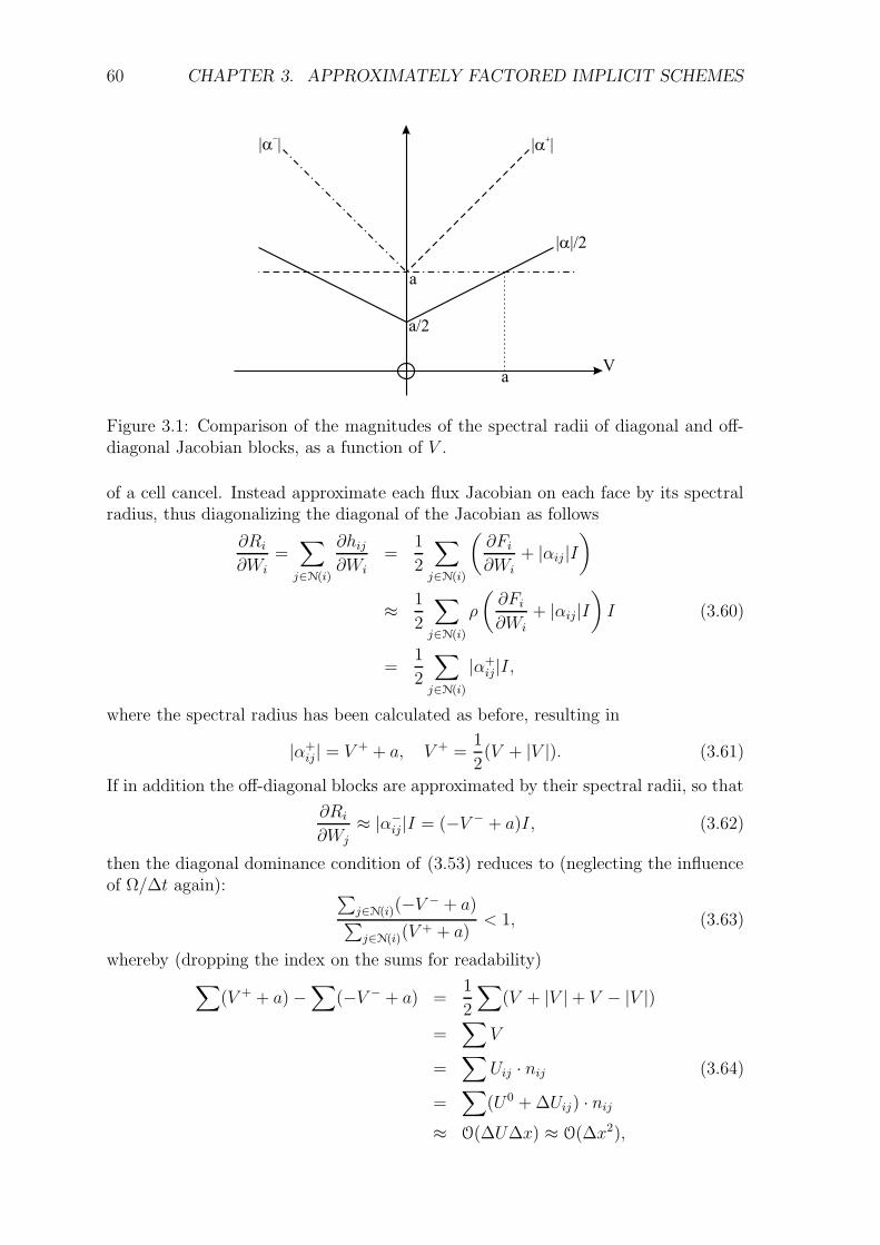
60 CHAPTER 3. APPROXIMATELY FACTORED IMPLICIT SCHEMES
V
a
a/2
a
|a|/2
|a |+
|a |-
Figure 3.1: Comparison of the magnitudes of the spectral radii of diagonal and off-diagonal Jacobian blocks, as a function of V .
of a cell cancel. Instead approximate each flux Jacobian on each face by its spectralradius, thus diagonalizing the diagonal of the Jacobian as follows
∂Ri
∂Wi=∑
j∈N(i)
∂hij∂Wi
=1
2
∑
j∈N(i)
(∂Fi∂Wi
+ |αij|I)
≈ 1
2
∑
j∈N(i)
ρ
(∂Fi∂Wi
+ |αij|I)I (3.60)
=1
2
∑
j∈N(i)
|α+ij|I,
where the spectral radius has been calculated as before, resulting in
|α+ij| = V + + a, V + =
1
2(V + |V |). (3.61)
If in addition the off-diagonal blocks are approximated by their spectral radii, so that
∂Ri
∂Wj
≈ |α−ij|I = (−V − + a)I, (3.62)
then the diagonal dominance condition of (3.53) reduces to (neglecting the influenceof Ω/∆t again): ∑
j∈N(i)(−V − + a)∑
j∈N(i)(V+ + a)
< 1, (3.63)
whereby (dropping the index on the sums for readability)∑
(V + + a)−∑
(−V − + a) =1
2
∑(V + |V |+ V − |V |)
=∑
V
=∑
Uij · nij (3.64)
=∑
(U0 + ∆Uij) · nij≈ O(∆U∆x) ≈ O(∆x2),
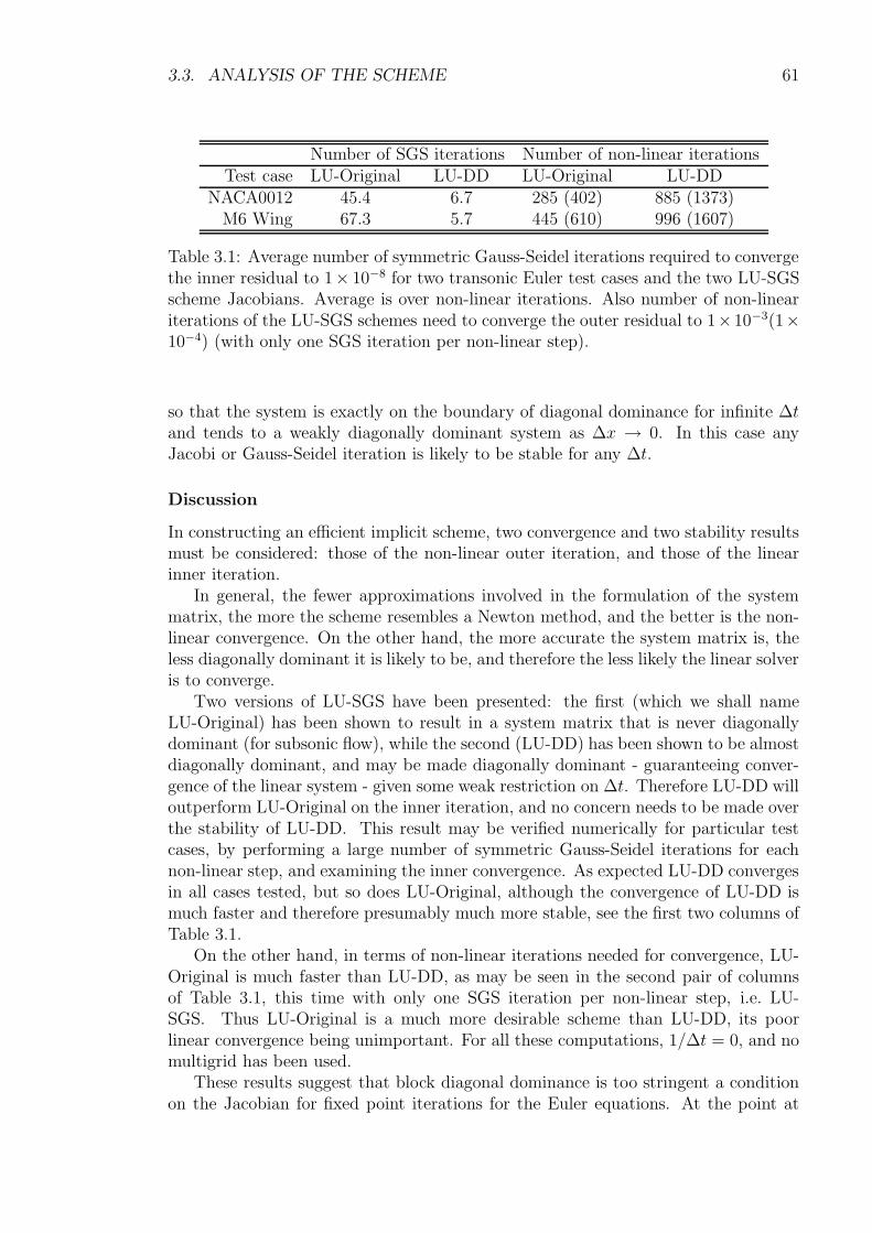
3.3. ANALYSIS OF THE SCHEME 61
Number of SGS iterations Number of non-linear iterationsTest case LU-Original LU-DD LU-Original LU-DD
NACA0012 45.4 6.7 285 (402) 885 (1373)M6 Wing 67.3 5.7 445 (610) 996 (1607)
Table 3.1: Average number of symmetric Gauss-Seidel iterations required to convergethe inner residual to 1× 10⁻⁸ for two transonic Euler test cases and the two LU-SGSscheme Jacobians. Average is over non-linear iterations. Also number of non-lineariterations of the LU-SGS schemes need to converge the outer residual to 1×10⁻³(1×10⁻⁴) (with only one SGS iteration per non-linear step).
so that the system is exactly on the boundary of diagonal dominance for infinite ∆tand tends to a weakly diagonally dominant system as ∆x → 0. In this case anyJacobi or Gauss-Seidel iteration is likely to be stable for any ∆t.
Discussion
In constructing an efficient implicit scheme, two convergence and two stability resultsmust be considered: those of the non-linear outer iteration, and those of the linearinner iteration.
In general, the fewer approximations involved in the formulation of the systemmatrix, the more the scheme resembles a Newton method, and the better is the non-linear convergence. On the other hand, the more accurate the system matrix is, theless diagonally dominant it is likely to be, and therefore the less likely the linear solveris to converge.
Two versions of LU-SGS have been presented: the first (which we shall nameLU-Original) has been shown to result in a system matrix that is never diagonallydominant (for subsonic flow), while the second (LU-DD) has been shown to be almostdiagonally dominant, and may be made diagonally dominant - guaranteeing conver-gence of the linear system - given some weak restriction on ∆t. Therefore LU-DD willoutperform LU-Original on the inner iteration, and no concern needs to be made overthe stability of LU-DD. This result may be verified numerically for particular testcases, by performing a large number of symmetric Gauss-Seidel iterations for eachnon-linear step, and examining the inner convergence. As expected LU-DD convergesin all cases tested, but so does LU-Original, although the convergence of LU-DD ismuch faster and therefore presumably much more stable, see the first two columns ofTable 3.1.
On the other hand, in terms of non-linear iterations needed for convergence, LU-Original is much faster than LU-DD, as may be seen in the second pair of columnsof Table 3.1, this time with only one SGS iteration per non-linear step, i.e. LU-SGS. Thus LU-Original is a much more desirable scheme than LU-DD, its poorlinear convergence being unimportant. For all these computations, 1/∆t = 0, and nomultigrid has been used.
These results suggest that block diagonal dominance is too stringent a conditionon the Jacobian for fixed point iterations for the Euler equations. At the point at
62 CHAPTER 3. APPROXIMATELY FACTORED IMPLICIT SCHEMES
which diagonal dominance is achieved, the Jacobian is too far removed from the trueJacobian for the non-linear iteration to be effective. Furthermore block diagonaldominance is generally a significantly looser condition than simple diagonal domi-nance (Feingold & Varga, 1962), and hence it may be asserted that diagonal dom-inance in general represents too stringent a requirement on the Jacobian for thesemethods.
Viscous Jacobian Approximation
Consider now the effect on the diagonal dominance of the approximation of (3.25),i.e. replacing the viscous Jacobians by their largest eigenvalue. This approximationincreases the diagonal dominance of the system matrix, under both definitions givenin Section 3.3.1, definition (3.42) trivially, and definition (3.44) since for a generalmatrix A
1
‖A−1‖ ≤ λi ≤ ‖A‖, ∀λieigenvalues of A, (3.65)
for all matrix norms ‖ · ‖. Hence under the arguments of Section 3.3.1 the innerSGS iteration is more likely to be stable, and to converge more rapidly. The diag-onal dominance may be further increased by approximating the off-diagonal viscousJacobians by their spectral radii as in (3.25), where here the second inequality of(3.65) is applied. However making such an approximation has the associated cost ofworsening the approximation of the Jacobian and therefore also worsening the rate ofconvergence of the non-linear iteration. The influence of this approximation on linearand non-linear convergence is evaluated numerically in Section 3.4.3.
Influence of Sum of Jacobians on Diagonal Dominance
One additional difficulty arising from the extension of the scheme to viscous terms isthat each block matrix of the Jacobian is the sum of at least two matrices: ∂f c/∂Wand ∂f v/∂W . The explicit expression for the spectral radius of this sum is toocomplex to be useful analytically, and so the spectral radius is approximated by thesum of the individual spectral radii in the scheme of Section 3.2. This approximationmay artifically reduce the diagonal dominance of the scheme; this is noteworthy as allthe other approximations we have made increase diagonal dominance. The problemis as follows:
For Hermitian matrices A and B with real eigenvalues λ1 ≥ λ2 ≥ · · · ≥ λn, theinequality
λk(A) + λn(B) ≤ λk(A+B) ≤ λk(A) + λ1(B), (3.66)
holds for k = 1, 2, · · · , n, see e.g. (Bhatia, 1997). A special case of this is
ρ (A +B) ≤ ρ (A) + ρ (B) , (3.67)
which is exactly what is needed to ensure that the sum of the spectral radii of theconvective and viscous Jacobians dominates the spectral radii of their sum. Result(3.66) is also true for any matrices A and B forming part of a real vector space whoseelements are matrices with real eigenvalues, and an analogous result holds for normalmatrices but no such result exists in general. The Jacobians under considerationsatisfy none of these conditions.
3.3. ANALYSIS OF THE SCHEME 63
One approach to bounding the eigenvalues of
A+B =∂f c
∂Wc+∂f v
∂Wc,
is to introduce a set of variables in which the convective and viscous Jacobians areboth symmetric (and hence normal). The parabolic symmetrizing variables Ws′ , andassociated change of basis matrices, are given in Appendix A.5. Let N = ∂Ws′/∂Wc,and A′ and B′ be the Jacobians in the variables Ws′, then
ρ(A +B) ≤ ‖A+B‖ =∥∥N−1A′N +N−1B′N
∥∥≤ ‖N−1‖ · ‖N‖ ‖A′‖+ ‖B′‖= κ(N) ρ(A′) + ρ(B′)= κ(N) ρ(A) + ρ(B)
where the definition of the condition number κ(A) = ‖A−1‖ · ‖A‖ ≥ 1 has been used,as well as the fact that ‖A‖ = ρ(A) for a normal matrix, and that the eigenvalues ofsimilar matrices are identical. Unfortunately κ(N) can be very large, in particular
κ(N) ≥ ρ(N)ρ(N−1) =max
√ρ3
p, ρ,√
ρ(γ−1)p
min√
ρ3
p, ρ,√
ρ(γ−1)p
,
where the eigenvalues here have been read directly from the diagonal of the triangularmatrix ∂Ws′/∂Wc. An alternative may be to formulate the implicit scheme entirelyin the variables Ws′ whereupon κ(N) = 1.
Further study is required to determine if the reduction of diagonal dominance dueto this approximation has an effect on the stability of the scheme.
3.3.2 Von Neumann Analysis of the Scheme
Von Neumann analysis, also known as Fourier analysis, is a technique for determin-ing the damping behaviour of a numerical scheme applied to a linear equation onan infinite periodic domain by considering each frequency component of the solutionseparately. Despite neglecting effects occurring in non-linear equations with bound-ary conditions, Fourier analysis has proven to be a useful tool in the study of thediscretization of such equations. A basic knowledge of von Neumann analysis hasbeen assumed in the following, see any introductory text on numerical analysis, rec-ommended is (Hirsch, 1989). In this section von Neumann analysis is applied to aconvection-diffusion equation with LU-SGS time stepping.
Modelling of the Residual
A model problem for the Navier-Stokes equations in two dimensions is the linear,scalar equation
∂ψ
∂t+ u
∂ψ
∂x+ v
∂ψ
∂y= µ
(∂2ψ
∂x2+∂2ψ
∂y2
)+ S · ψ, (3.68)
64 CHAPTER 3. APPROXIMATELY FACTORED IMPLICIT SCHEMES
i.e. a convection-diffusion equation with constant coefficients and a source term. Con-sider a finite uniform rectangular mesh aligned with the coordinate axes, with a cellspacing ∆x and ∆y. A discretization of (3.68) on this mesh with a general formulationof the convective terms and central differencing for the viscous terms is
Z · ψij = ZC · ψ− Λµx(ψi−1j − 2ψij + ψi+1j)
− Λµy(ψij−1 − 2ψij + ψij+1) (3.69)
− S · ψij,
where Z is the Fourier symbol corresponding to the residual R of (3.68), and Λ arethe eigenvalues of the spatial operators:
Λx = u∆y, Λy = v∆x,
Λµx = µ∆y
∆x, Λµy = µ
∆x
∆y. (3.70)
It is expected that the combination of LHS and RHS discretizations plays an im-portant role in the damping properties of the implicit scheme, hence several RHSdiscretizations are considered. A second-order upwind scheme is modelled by
ZCU · ψij =1
2Λx(3ψij − 4ψi−1j + ψi−2j)
+1
2Λy(3ψij − 4ψij−1 + ψij−2), (3.71)
but a discretization that corresponds better to the JST scheme is central differencingwith a 4th-order dissipation term,
ZCC · ψij =1
2Λx(ψi+1j − ψi−1j) +
1
2Λy(ψij+1 − ψij−1)
+ Λxdx(ψi+2j − 4ψi+1j + 6ψij − 4ψi−1j + ψi−2j) (3.72)
+ Λydy(ψij+2 − 4ψij+1 + 6ψij − 4ψij−1 + ψij−2),
where dx, dy are the dissipation coefficients. A deficiency of this model is that thedissipation is calculated independently for each coordinate direction, which is typi-cally not the case for unstructured flow solvers. The Tau-code for example uses anon-divided Laplacian to approximate a second-order dissipation, and a Laplacian ofa Laplacian for fourth-order dissipation. A corresponding operator in this context is
D2nd · ψij = ∆y(ψi+1j − 2ψij + ψi−1j) + ∆x(ψij+1 − 2ψij + ψij−1), (3.73)
from which a fourth-order difference operator may be constructed
D4th · ψij = ΛxD2nd · (ψi+1j − 2ψij + ψi−1j)
+ ΛyD2nd · (ψij+1 − 2ψij + ψij−1), (3.74)
resulting in a convective flux of
ZCC,iso · ψij =1
2Λx(ψi+1j − ψi−1j) +
1
2Λy(ψij+1 − ψij−1)
+1
2dxyD4th · ψij,
3.3. ANALYSIS OF THE SCHEME 65
where the single dissipation coefficient is dxy.The Fourier symbols of these operators are obtained by substituting for a harmonic
solution with amplitude ψψ = ψeI(iφx+jφy), (3.75)
where the phase angles φx, φy vary in the range [−π, π), and thereby cover all fre-quencies up to the highest frequency representable on the mesh. The Fourier symbolsof the upwind and directional central scheme are then
ZCU = Λx
I sinφx(2− cosφx) + (1− cos φx)
2
+ Λy
I sinφy(2− cosφy) + (1− cosφy)
2, (3.76)
ZCC = Λx
I sinφx + 4dx(1− cosφx)
2
+ Λy
I sinφy + 4dy(1− cosφy)
2, (3.77)
while the Fourier symbol of the non-directional central scheme may be constructed byconsidering the symbol of the second-order dissipation (3.73) with an offset (λx, λy)
D(λx,λy)2nd = ∆y
eI((λx+1)φx+λyφy) − 2eI(λxφx+λyφy) + eI((λx−1)φx+λyφy)
+ ∆x
eI(λxφx+(λy+1)φy) − 2eI(λxφx+λyφy) + eI(λxφx+(λy−1)φy), (3.78)
using which the symbol of the fourth-order dissipation (3.74) is
D4th = Λx
(D
(1,0)2nd − 2D
(0,0)2nd + D
(−1,0)2nd
)
+ Λy
(D
(0,1)2nd − 2D
(0,0)2nd + D
(0,−1)2nd
), (3.79)
and therefore the symbol of the central scheme with isotropic dissipation is
ZCC,iso = I(sinφx + sin φy) +1
2dxyD4th. (3.80)
Modelling of LU-SGS
Note that because the model equation is linear, the error satisfies the same equationas the solution. Any explicit or implicit scheme used to solve the discretized modelequation will be stable if the amplitude ψ of every harmonic of the error does notgrow in time, that is if
|g| =∣∣∣∣∣ψn+1
ψn
∣∣∣∣∣ ≤ 1 ∀φx, φy, (3.81)
where g is known as the amplification factor or damping factor of the combined time-space discretization.
For the problem on the structured grid the LHS of the implicit system (3.8) maybe written
I
∆t+∂R
∂ψ
=
I
∆t+ A+B + Aµ +Bµ + T
, (3.82)
where A, B are the convective Jacobians, Aµ, Bµ the viscous Jacobians and T thesource term Jacobian. The discrepancy between the fluxes and the Jacobians in thetrue scheme is taken into account by using a first-order upwind discretization for
66 CHAPTER 3. APPROXIMATELY FACTORED IMPLICIT SCHEMES
A and B, as well as an implicit damping coefficient ωrelax for the dissipation. Theviscous Jacobians are taken to be exact with respect to the RHS. Corresponding to(3.23) it may be shown that
A± =1
2(Λx ± ωrelax|Λx|) ,
B± =1
2(Λy ± ωrelax|Λy|) ,
Aµ = Λµx (3.83)
Bµ = Λµy
T = S
where + and − denote differentials with respect to ψ at points i+ 1 / j+ 1 and i− 1/ j − 1 respectively. If the grid points are lexicographically ordered then the matrixoperators are
L · ψij = −A+ψi−1j −B+ψij−1 − Aµψi−1j − Bµψij−1,
U · ψij = A−ψi+1j +B−ψij+1 − Aµψi+1j − Bµψij+1, (3.84)
D · ψij =
1
∆t+ ωrelax (|Λx|+ |Λy|) + 2(Aµ +Bµ) + T
ψij,
with Fourier symbols
L = −A+e−Iφx −B+e−Iφy − Aµe−Iφx −Bµe−Iφy ,
U = A−eIφx +B−eIφy − AµeIφx − BµeIφy , (3.85)
D =
1
∆t+ ωrelax (|Λx|+ |Λy|) + 2(Aµ +Bµ) + T
.
By noting that the Fourier symbol of an inverse operator is the reciprocal of theFourier symbol of the original operator,
L−1 =1
L, (3.86)
the amplification factor of LU-SGS may be deduced directly from (3.12), using (3.85):
|g| =∣∣∣∣∣1−
Z
(L+ D)D−1(U + D)
∣∣∣∣∣ . (3.87)
Influence of the Source Term
The presence of the source term S in the model equation (3.68) is an attempt torepresent the source terms occurring in the turbulence equations, and has been studiedextensively in the context of von Neumann analysis (Faßbender, 2003). The coefficientS is taken to be constant, i.e. uniform production or destruction over the entiredomain. This equation differs slightly from the typical convection diffusion modelequation, and so we consider firstly some of its properties.
3.3. ANALYSIS OF THE SCHEME 67
The exact solution of linear equation on a periodic domain may be found bysubstituting in a Fourier mode and solving for the coefficient a of t in the exponent.A two parameter family of exact solutions of the scalar model equation is then
ψ = ψ exp
I
(x
∆xφx +
y
∆yφy
)+ at
,
a = −I(uφx∆x
+ vφy∆y
)− µ
(φ2x
∆x2+
φ2y
∆y2
)+ S,
where x and y have been normalized using ∆x and ∆y such that when φx = π orφy = π the mode’s frequency corresponds to the highest frequency representable onthe mesh. By Fourier’s Theorem these are all solutions - up to linear superposition -of the model equation. As may be immediately seen, a mode grows exponentially intime if
S
µ>
φ2x
∆x2+
φ2y
∆y2, (3.88)
i.e. for an ellipse in the phase plane, and is otherwise stable. A consequence is thatfor positive S the solution always grows unboundedly for sufficiently low frequencies.Note that due to the linearity of the model equation, any error in an approximatesolution satisfies the same equation as the solution itself, and hence also grows expo-nentially for the frequencies specified by condition (3.88).
Given that the model equation itself is “unstable” for these low frequencies, itis unreasonable to expect numerical methods to be stable there, and indeed Fourieranalysis shows that they are typically not. Figure 3.2 shows the damping factor |g| fora 4-stage Runge-Kutta scheme for the model equation with source term; in particularS = 1/20, µ = 1/10, ∆x = 1 and ∆y = 2/5. In the centre of the contour plot itcan be seen that the amplification factor increases above 1, taking a maximum valueat (φx, φy) = (0, 0). The central, bold-dashed ellipse shows the limit of the stabilityregion of the model equation, as given by (3.88). It can be seen that the method isonly unstable when the model equation itself has an unbounded solution.
In this case the natural criteria for judging the stability of a numerical method,namely that the amplifaction factor is always less than or equal to one, is no longersuitable. The only alternative is to suggest that a method be considered stable if theamplification factor in the region of stability of the model problem is always less thanone. Such a property we will call compatibly stable. Then the method of Figure 3.2 isnot stable, but it is compatibly stable, as the scheme only amplifies the error wherethe model equation does.
It is of interest to determine for which values of S, µ and ∆t the methods describedabove are compatibly stable, which may be done by determining at which frequenciesthe amplification factor passes through 1. For compatible stability in one dimensionwe require that
|g(φ)| ≤ 1 for all φ ∈[
∆x
√S
µ, π
].
Since in the cases above |g| is a continuously differentiable function of φ, and variescontinuously with S, µ and ∆t, it can only change from being stable to unstable when
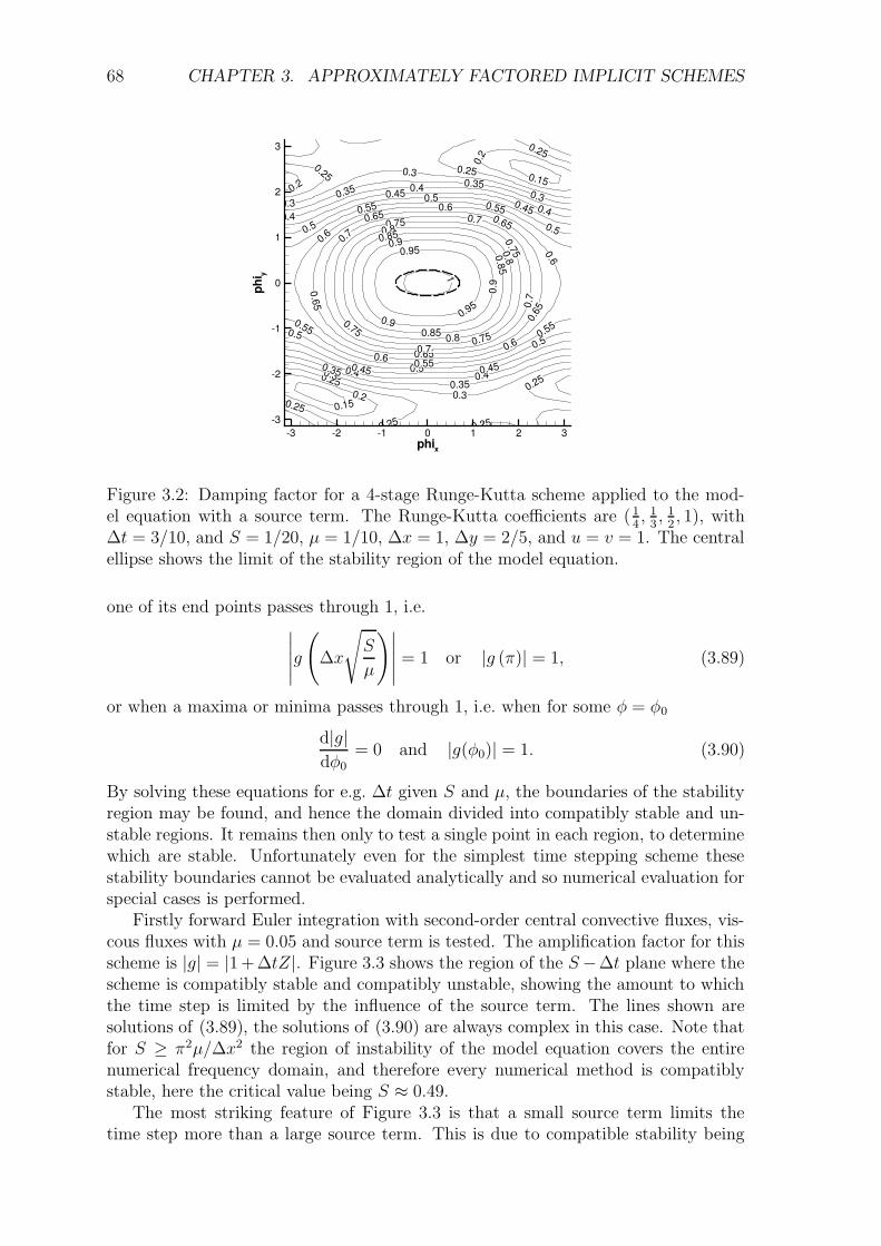
68 CHAPTER 3. APPROXIMATELY FACTORED IMPLICIT SCHEMES
0.15
0.15
0.2
0.2
0.2
0.25
0.25
0.25
0.25 0.25
0.25
0.25
0.250.3
0.3
0.3
0.3
0.3
0.350.35
0.350.35
0.4 0.4
0.4
0.4
0.4
0.45 0.45
0.450.45
0.5
0.5
0.5
0.5
0.5
0.5
0.55
0.55
0.55
0.55 0.55
0.60.6
0.6
0.6
0.6
0.65
0.65
0.650.65
0.65
0.7
0.7
0.7
0.7
0.750.75
0.75
0.75
0.8
0.8
0.8
0.85
0.85
0.85
0.9
0.9
0.9
0.95
0.95
1phix
phi y
-3 -2 -1 0 1 2 3-3
-2
-1
0
1
2
3
Figure 3.2: Damping factor for a 4-stage Runge-Kutta scheme applied to the mod-el equation with a source term. The Runge-Kutta coefficients are ( 1
4, 1
3, 1
2, 1), with
∆t = 3/10, and S = 1/20, µ = 1/10, ∆x = 1, ∆y = 2/5, and u = v = 1. The centralellipse shows the limit of the stability region of the model equation.
one of its end points passes through 1, i.e.∣∣∣∣∣g(
∆x
√S
µ
)∣∣∣∣∣ = 1 or |g (π)| = 1, (3.89)
or when a maxima or minima passes through 1, i.e. when for some φ = φ0
d|g|dφ0
= 0 and |g(φ0)| = 1. (3.90)
By solving these equations for e.g. ∆t given S and µ, the boundaries of the stabilityregion may be found, and hence the domain divided into compatibly stable and un-stable regions. It remains then only to test a single point in each region, to determinewhich are stable. Unfortunately even for the simplest time stepping scheme thesestability boundaries cannot be evaluated analytically and so numerical evaluation forspecial cases is performed.
Firstly forward Euler integration with second-order central convective fluxes, vis-cous fluxes with µ = 0.05 and source term is tested. The amplification factor for thisscheme is |g| = |1 + ∆tZ|. Figure 3.3 shows the region of the S−∆t plane where thescheme is compatibly stable and compatibly unstable, showing the amount to whichthe time step is limited by the influence of the source term. The lines shown aresolutions of (3.89), the solutions of (3.90) are always complex in this case. Note thatfor S ≥ π2µ/∆x2 the region of instability of the model equation covers the entirenumerical frequency domain, and therefore every numerical method is compatiblystable, here the critical value being S ≈ 0.49.
The most striking feature of Figure 3.3 is that a small source term limits thetime step more than a large source term. This is due to compatible stability being
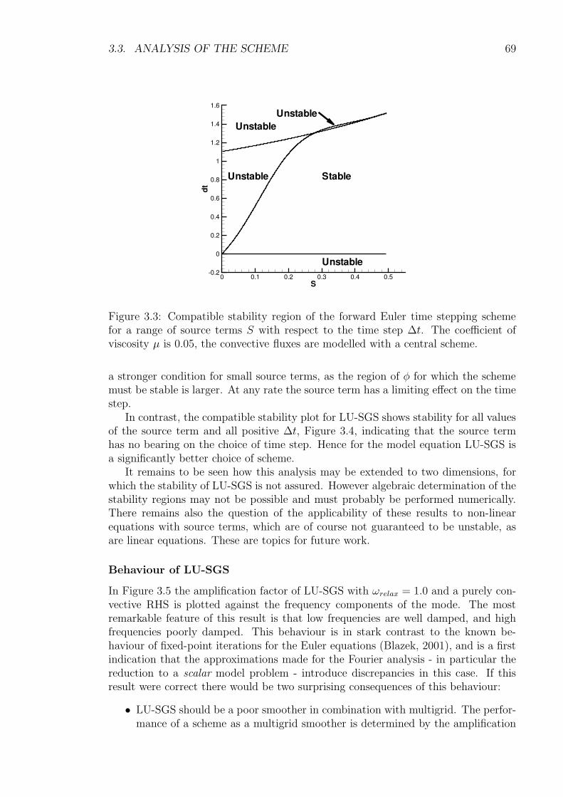
3.3. ANALYSIS OF THE SCHEME 69
S
dt
0 0.1 0.2 0.3 0.4 0.5-0.2
0
0.2
0.4
0.6
0.8
1
1.2
1.4
1.6
Stable
Unstable
Unstable
Unstable
Unstable
Figure 3.3: Compatible stability region of the forward Euler time stepping schemefor a range of source terms S with respect to the time step ∆t. The coefficient ofviscosity µ is 0.05, the convective fluxes are modelled with a central scheme.
a stronger condition for small source terms, as the region of φ for which the schememust be stable is larger. At any rate the source term has a limiting effect on the timestep.
In contrast, the compatible stability plot for LU-SGS shows stability for all valuesof the source term and all positive ∆t, Figure 3.4, indicating that the source termhas no bearing on the choice of time step. Hence for the model equation LU-SGS isa significantly better choice of scheme.
It remains to be seen how this analysis may be extended to two dimensions, forwhich the stability of LU-SGS is not assured. However algebraic determination of thestability regions may not be possible and must probably be performed numerically.There remains also the question of the applicability of these results to non-linearequations with source terms, which are of course not guaranteed to be unstable, asare linear equations. These are topics for future work.
Behaviour of LU-SGS
In Figure 3.5 the amplification factor of LU-SGS with ωrelax = 1.0 and a purely con-vective RHS is plotted against the frequency components of the mode. The mostremarkable feature of this result is that low frequencies are well damped, and highfrequencies poorly damped. This behaviour is in stark contrast to the known be-haviour of fixed-point iterations for the Euler equations (Blazek, 2001), and is a firstindication that the approximations made for the Fourier analysis - in particular thereduction to a scalar model problem - introduce discrepancies in this case. If thisresult were correct there would be two surprising consequences of this behaviour:
• LU-SGS should be a poor smoother in combination with multigrid. The perfor-mance of a scheme as a multigrid smoother is determined by the amplification
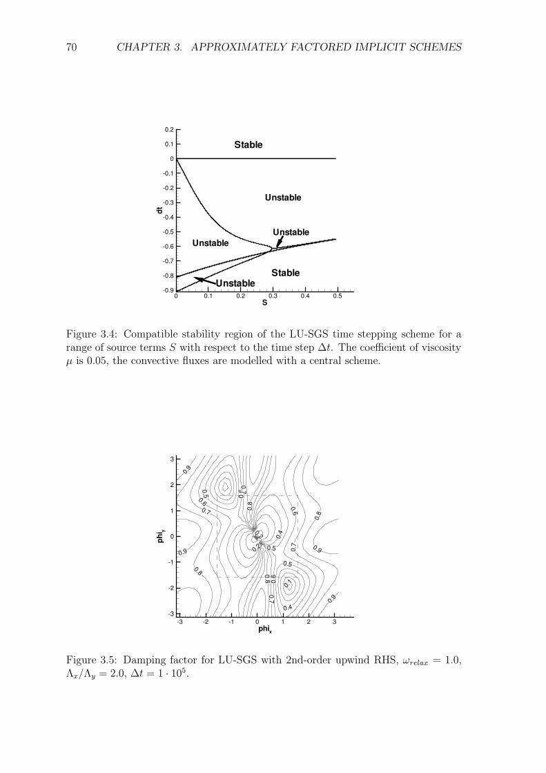
70 CHAPTER 3. APPROXIMATELY FACTORED IMPLICIT SCHEMES
S
dt
0 0.1 0.2 0.3 0.4 0.5-0.9
-0.8
-0.7
-0.6
-0.5
-0.4
-0.3
-0.2
-0.1
0
0.1
0.2
Stable
Unstable
Unstable
Unstable
Stable
Unstable
Figure 3.4: Compatible stability region of the LU-SGS time stepping scheme for arange of source terms S with respect to the time step ∆t. The coefficient of viscosityµ is 0.05, the convective fluxes are modelled with a central scheme.
0.1
0.2
0.2 0.4
0.4
0.5
0.5
0.5
0.6
0.6
0.6
0.6
0.7
0.70.
7
0.7
0.8
0.8
0.8
0.8
0.9
0.9
0.9
0.9
phix
phi y
-3 -2 -1 0 1 2 3-3
-2
-1
0
1
2
3
Figure 3.5: Damping factor for LU-SGS with 2nd-order upwind RHS, ωrelax = 1.0,Λx/Λy = 2.0, ∆t = 1 · 105.
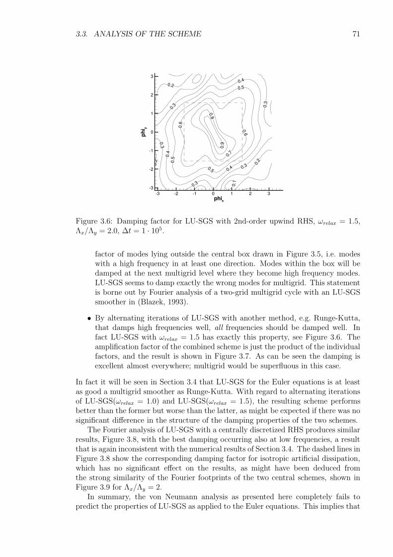
3.3. ANALYSIS OF THE SCHEME 71
0.1
0.2
0.2
0.2
0.3
0.3 0.3
0.3
0.30.4
0.4
0.4
0.5
0.5
0.5
0.6
0.6
0.7
0.8
0.9
phix
phi y
-3 -2 -1 0 1 2 3-3
-2
-1
0
1
2
3
Figure 3.6: Damping factor for LU-SGS with 2nd-order upwind RHS, ωrelax = 1.5,Λx/Λy = 2.0, ∆t = 1 · 105.
factor of modes lying outside the central box drawn in Figure 3.5, i.e. modeswith a high frequency in at least one direction. Modes within the box will bedamped at the next multigrid level where they become high frequency modes.LU-SGS seems to damp exactly the wrong modes for multigrid. This statementis borne out by Fourier analysis of a two-grid multigrid cycle with an LU-SGSsmoother in (Blazek, 1993).
• By alternating iterations of LU-SGS with another method, e.g. Runge-Kutta,that damps high frequencies well, all frequencies should be damped well. Infact LU-SGS with ωrelax = 1.5 has exactly this property, see Figure 3.6. Theamplification factor of the combined scheme is just the product of the individualfactors, and the result is shown in Figure 3.7. As can be seen the damping isexcellent almost everywhere; multigrid would be superfluous in this case.
In fact it will be seen in Section 3.4 that LU-SGS for the Euler equations is at leastas good a multigrid smoother as Runge-Kutta. With regard to alternating iterationsof LU-SGS(ωrelax = 1.0) and LU-SGS(ωrelax = 1.5), the resulting scheme performsbetter than the former but worse than the latter, as might be expected if there was nosignificant difference in the structure of the damping properties of the two schemes.
The Fourier analysis of LU-SGS with a centrally discretized RHS produces similarresults, Figure 3.8, with the best damping occurring also at low frequencies, a resultthat is again inconsistent with the numerical results of Section 3.4. The dashed lines inFigure 3.8 show the corresponding damping factor for isotropic artificial dissipation,which has no significant effect on the results, as might have been deduced fromthe strong similarity of the Fourier footprints of the two central schemes, shown inFigure 3.9 for Λx/Λy = 2.
In summary, the von Neumann analysis as presented here completely fails topredict the properties of LU-SGS as applied to the Euler equations. This implies that
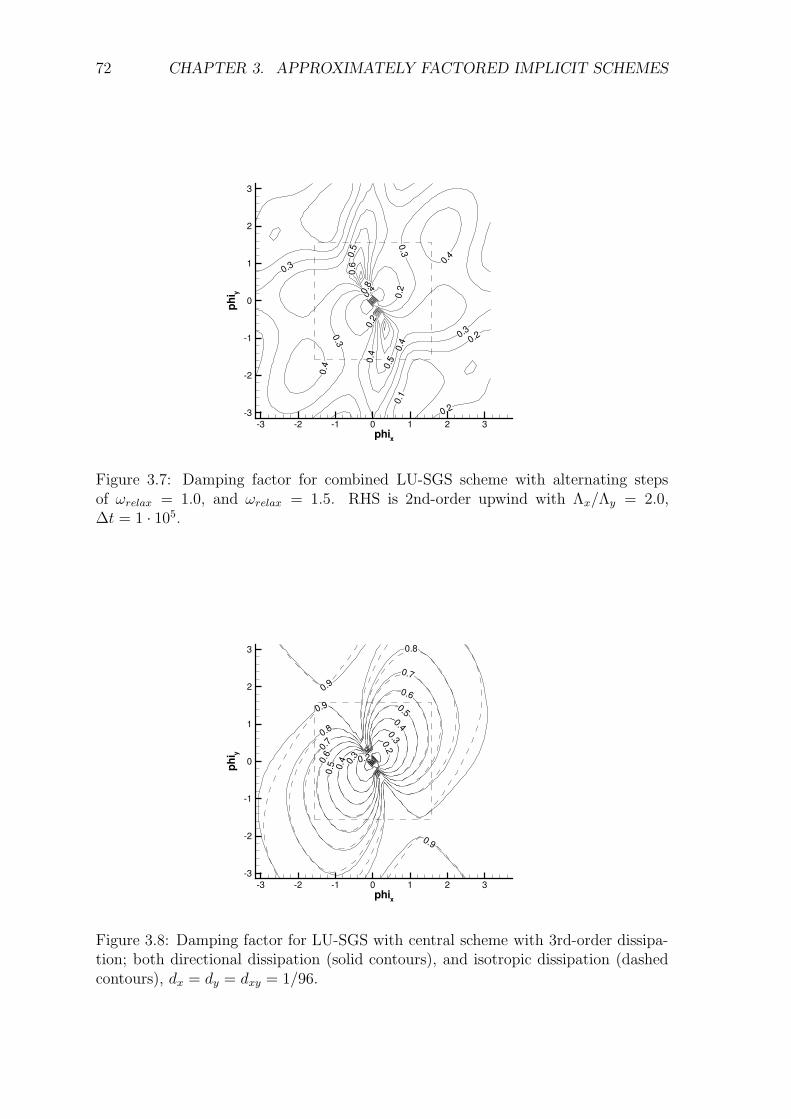
72 CHAPTER 3. APPROXIMATELY FACTORED IMPLICIT SCHEMES
0.1
0.2
0.2
0.2
0.2
0.3
0.3
0.3
0.30.
4
0.4
0.4
0.4
0.4
0.5
0.5
0.6
0.8
phix
phi y
-3 -2 -1 0 1 2 3-3
-2
-1
0
1
2
3
Figure 3.7: Damping factor for combined LU-SGS scheme with alternating stepsof ωrelax = 1.0, and ωrelax = 1.5. RHS is 2nd-order upwind with Λx/Λy = 2.0,∆t = 1 · 105.
0.9
0.9
0.8
0.70.
60.
5 0.4 0.30.2
0.8
0.7
0.60.5
0.40.30.2
0.9
phix
phi y
-3 -2 -1 0 1 2 3-3
-2
-1
0
1
2
3
Figure 3.8: Damping factor for LU-SGS with central scheme with 3rd-order dissipa-tion; both directional dissipation (solid contours), and isotropic dissipation (dashedcontours), dx = dy = dxy = 1/96.
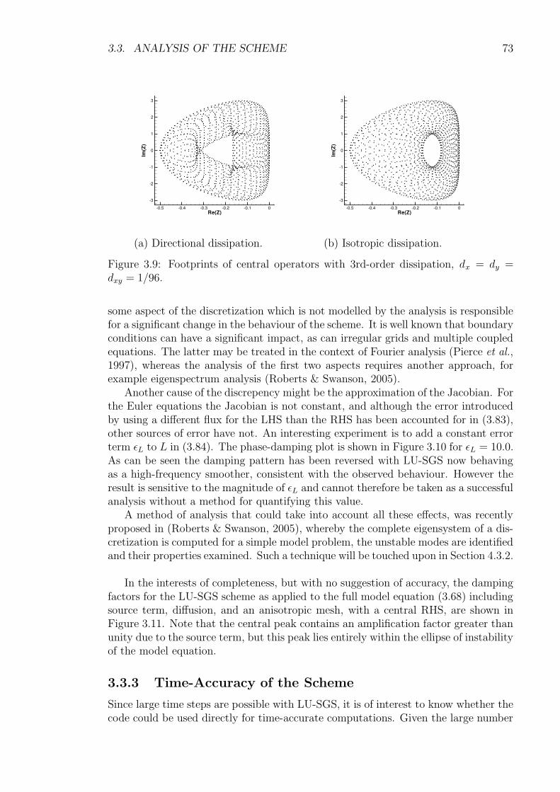
3.3. ANALYSIS OF THE SCHEME 73
Re(Z)
Im(Z
)
-0.5 -0.4 -0.3 -0.2 -0.1 0
-3
-2
-1
0
1
2
3
(a) Directional dissipation.
Re(Z)
Im(Z
)
-0.5 -0.4 -0.3 -0.2 -0.1 0
-3
-2
-1
0
1
2
3
(b) Isotropic dissipation.
Figure 3.9: Footprints of central operators with 3rd-order dissipation, dx = dy =dxy = 1/96.
some aspect of the discretization which is not modelled by the analysis is responsiblefor a significant change in the behaviour of the scheme. It is well known that boundaryconditions can have a significant impact, as can irregular grids and multiple coupledequations. The latter may be treated in the context of Fourier analysis (Pierce et al.,1997), whereas the analysis of the first two aspects requires another approach, forexample eigenspectrum analysis (Roberts & Swanson, 2005).
Another cause of the discrepency might be the approximation of the Jacobian. Forthe Euler equations the Jacobian is not constant, and although the error introducedby using a different flux for the LHS than the RHS has been accounted for in (3.83),other sources of error have not. An interesting experiment is to add a constant errorterm εL to L in (3.84). The phase-damping plot is shown in Figure 3.10 for εL = 10.0.As can be seen the damping pattern has been reversed with LU-SGS now behavingas a high-frequency smoother, consistent with the observed behaviour. However theresult is sensitive to the magnitude of εL and cannot therefore be taken as a successfulanalysis without a method for quantifying this value.
A method of analysis that could take into account all these effects, was recentlyproposed in (Roberts & Swanson, 2005), whereby the complete eigensystem of a dis-cretization is computed for a simple model problem, the unstable modes are identifiedand their properties examined. Such a technique will be touched upon in Section 4.3.2.
In the interests of completeness, but with no suggestion of accuracy, the dampingfactors for the LU-SGS scheme as applied to the full model equation (3.68) includingsource term, diffusion, and an anisotropic mesh, with a central RHS, are shown inFigure 3.11. Note that the central peak contains an amplification factor greater thanunity due to the source term, but this peak lies entirely within the ellipse of instabilityof the model equation.
3.3.3 Time-Accuracy of the Scheme
Since large time steps are possible with LU-SGS, it is of interest to know whether thecode could be used directly for time-accurate computations. Given the large number
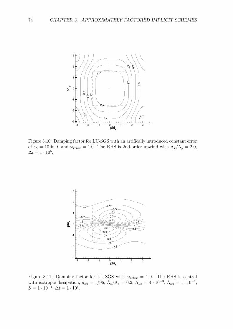
74 CHAPTER 3. APPROXIMATELY FACTORED IMPLICIT SCHEMES
0.3
0.5
0.5
0.6
0.6
0.7
0.7
0.7
0.8
0.8
0.9
0.9
phix
phi y
-3 -2 -1 0 1 2 3-3
-2
-1
0
1
2
3
Figure 3.10: Damping factor for LU-SGS with an artifically introduced constant errorof εL = 10 in L and ωrelax = 1.0. The RHS is 2nd-order upwind with Λx/Λy = 2.0,∆t = 1 · 105.
0.7 0.60.5
0.40.30.2 0.7
0.9
0.8
0.70.6
0.50.4
0.3
0.2
0.9
0.7
0.8
phix
phi y
-3 -2 -1 0 1 2 3-3
-2
-1
0
1
2
3
Figure 3.11: Damping factor for LU-SGS with ωrelax = 1.0. The RHS is centralwith isotropic dissipation, dxy = 1/96, Λx/Λy = 0.2, Λµx = 4 · 10−3, Λµy = 1 · 10−1,S = 1 · 10−4, ∆t = 1 · 105.
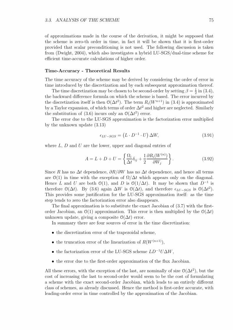
3.3. ANALYSIS OF THE SCHEME 75
of approximations made in the course of the derivation, it might be supposed thatthe scheme is zero-th order in time, in fact it will be shown that it is first-orderprovided that scalar preconditioning is not used. The following discussion is takenfrom (Dwight, 2004), which also investigates a hybrid LU-SGS/dual-time scheme forefficient time-accurate calculations of higher order.
Time-Accuracy - Theoretical Results
The time accuracy of the scheme may be derived by considering the order of error intime introduced by the discretization and by each subsequent approximation thereof.
The time discretization may be chosen to be second-order by setting β = 12
in (3.4),the backward difference formula on which the scheme is based. The error incurred bythe discretization itself is then O(∆t2). The term Ri(W
n+1) in (3.4) is approximatedby a Taylor expansion, of which terms of order ∆t2 and higher are neglected. Similarlythe substitution of (3.6) incurs only an O(∆t2) error.
The error due to the LU-SGS approximation is the factorization error multipliedby the unknown update (3.13)
εLU−SGS =(L ·D−1 · U
)∆W, (3.91)
where L, D and U are the lower, upper and diagonal entries of
A = L +D + U =
Ωi
∆tδij +
1
2
∂Ri(W(n))
∂Wj
. (3.92)
Since R has no ∆t dependence, ∂R/∂W has no ∆t dependence, and hence all termsare O(1) in time with the exception of Ω/∆t which appears only on the diagonal.Hence L and U are both O(1), and D is O(1/∆t). It may be shown that D−1 istherefore O(∆t). By (3.6) again ∆W is O(∆t), and therefore εLU−SGS is O(∆t2).This provides some justification for the LU-SGS approximation itself: as the timestep tends to zero the factorization error also disappears.
The final approximation is to substitute the exact Jacobian of (3.7) with the first-order Jacobian, an O(1) approximation. This error is then multiplied by the O(∆t)unknown update, giving a composite O(∆t) error.
In summary there are four sources of error in the time discretization:
• the discretization error of the trapezoidal scheme,
• the truncation error of the linearization of R(W (n+1)),
• the factorization error of the LU-SGS scheme LD−1U∆W ,
• the error due to the first-order approximation of the flux Jacobian.
All these errors, with the exception of the last, are nominally of size O(∆t2), but thecost of increasing the last to second-order would seem to be the cost of formulatinga scheme with the exact second-order Jacobian, which leads to an entirely differentclass of schemes, as already discussed. Hence the method is first-order accurate, withleading-order error in time controlled by the approximation of the Jacobian.
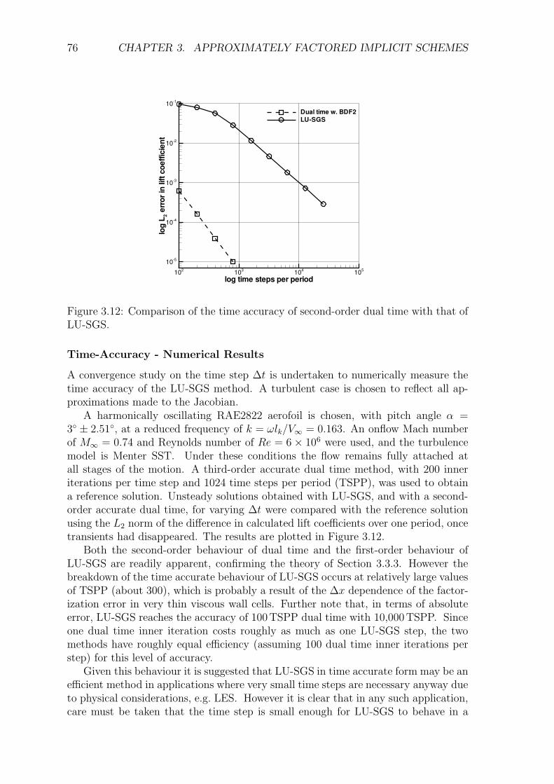
76 CHAPTER 3. APPROXIMATELY FACTORED IMPLICIT SCHEMES
log time steps per period
log
L 2er
rori
nlif
tcoe
ffici
ent
102 103 104 105
10-5
10-4
10-3
10-2
10-1
Dual time w. BDF2LU-SGS
Figure 3.12: Comparison of the time accuracy of second-order dual time with that ofLU-SGS.
Time-Accuracy - Numerical Results
A convergence study on the time step ∆t is undertaken to numerically measure thetime accuracy of the LU-SGS method. A turbulent case is chosen to reflect all ap-proximations made to the Jacobian.
A harmonically oscillating RAE2822 aerofoil is chosen, with pitch angle α =3 ± 2.51, at a reduced frequency of k = ωlk/V∞ = 0.163. An onflow Mach numberof M∞ = 0.74 and Reynolds number of Re = 6× 10⁶ were used, and the turbulencemodel is Menter SST. Under these conditions the flow remains fully attached atall stages of the motion. A third-order accurate dual time method, with 200 inneriterations per time step and 1024 time steps per period (TSPP), was used to obtaina reference solution. Unsteady solutions obtained with LU-SGS, and with a second-order accurate dual time, for varying ∆t were compared with the reference solutionusing the L2 norm of the difference in calculated lift coefficients over one period, oncetransients had disappeared. The results are plotted in Figure 3.12.
Both the second-order behaviour of dual time and the first-order behaviour ofLU-SGS are readily apparent, confirming the theory of Section 3.3.3. However thebreakdown of the time accurate behaviour of LU-SGS occurs at relatively large valuesof TSPP (about 300), which is probably a result of the ∆x dependence of the factor-ization error in very thin viscous wall cells. Further note that, in terms of absoluteerror, LU-SGS reaches the accuracy of 100 TSPP dual time with 10,000 TSPP. Sinceone dual time inner iteration costs roughly as much as one LU-SGS step, the twomethods have roughly equal efficiency (assuming 100 dual time inner iterations perstep) for this level of accuracy.
Given this behaviour it is suggested that LU-SGS in time accurate form may be anefficient method in applications where very small time steps are necessary anyway dueto physical considerations, e.g. LES. However it is clear that in any such application,care must be taken that the time step is small enough for LU-SGS to behave in a
3.4. NUMERICAL RESULTS 77
time accurate manner.
3.4 Numerical Results
The purpose of this section is twofold. Firstly it is demonstrated that, after the twomajor approximations of LUSGS: (a) considering only a first-order Jacobian, and (b)solving the linear system with one SGS iteration, the influence of the subsequentapproximations made in Section 3.2 (in particular the use of the Lax-Friedrichs fluxand the replacement of the viscous flux Jacobians by their eigenvalues) on the non-linear convergence is minor.
Secondly it is demonstrated that the algorithm thus derived may be applied toa large case of practical engineering interest. Runge-Kutta with residual smoothingand multigrid serves as a reference algorithm throughout, representing as it does thenext-best available algorithm.
Within this section the convergence of various algorithms must be compared. Inorder that performance may be uniformly judged - and to avoid numerous conver-gence plots - some metric for speed of convergence must be decided upon. A commonmetric is the convergence rate, which is typically constant as the solution asymptoti-cally approaches the exact solution. However, given that cases of engineering interesttypically involve convergence of no more than four orders of magnitude, and thatconvergence behaviour in this range tends to be highly non-uniform, the convergencerate varies considerably. Instead the following measure is used: the number of iter-ations (or normalized CPU time) from the beginning of the calculation required forthe normalized residual to drop and remain below 1×10⁻³ and 1×10⁻⁴. The residualin all cases is normalized against the residual calculated on the first step.
A second metric of the algorithm is taken, which has already been used in Sec-tion 3.3.1: the number of linear iterations of SGS needed to drive the (also normalized)linear residual below 1× 10⁻⁸. This provides a measure of the relative diagonal dom-inance of the Jacobian, or the relative stability of the Gauss-Seidel iteration, for twodifferent methods. It will be used to verify the theoretical results of Section 3.3.
3.4.1 Approximations of the Jacobian
In Section 3.2 it was discussed how the use of a Jacobian derived from first-orderfluxes reduces the memory requirements and complexity of the scheme. In contrastsome of the other approximations made are useful but not essential. For examplethe choice of the Lax-Friedrichs flux, which reduces the diagonal-block entries of theJacobian to diagonal matrices, could be replaced by a Roe flux, whose Jacobian con-tains significantly more information about the flow. Hence each such approximationis evaluated numerically for its effect on the linear and non-linear convergence rates.
First however it is useful to observe the effect the reduction of the order of theJacobian from second to first has on the convergence of the non-linear system, in-dependently of other Jacobian approximations and given exact solution of the inter-mediate linear systems. Refer to Section 1.1 for an overview of the types of implicitmethods discussed here.
Two implicit schemes, one using exact 1st-order Jacobians, and the other usingexact 2nd-order Jacobians are constructed in a Jacobian-Free manner using finite
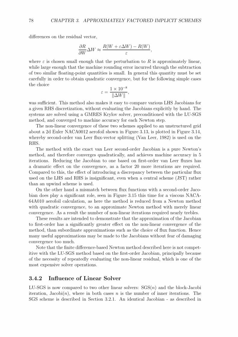
78 CHAPTER 3. APPROXIMATELY FACTORED IMPLICIT SCHEMES
differences on the residual vector,
∂R
∂W∆W ≈ R(W + ε∆W )− R(W )
ε,
where ε is chosen small enough that the perturbation to R is approximately linear,while large enough that the machine rounding error incurred through the subtractionof two similar floating-point quantities is small. In general this quantity must be setcarefully in order to obtain quadratic convergence, but for the following simple casesthe choice
ε =1× 10⁻⁸
‖∆W‖ ,
was sufficient. This method also makes it easy to compare various LHS Jacobians fora given RHS discretization, without evaluating the Jacobians explicitly by hand. Thesystems are solved using a GMRES Krylov solver, preconditioned with the LU-SGSmethod, and converged to machine accuracy for each Newton step.
The non-linear convergence of these two schemes applied to an unstructured gridabout a 2d Euler NACA0012 aerofoil shown in Figure 3.13, is plotted in Figure 3.14,whereby second-order van Leer flux-vector splitting (Van Leer, 1982) is used on theRHS.
The method with the exact van Leer second-order Jacobian is a pure Newton’smethod, and therefore converges quadratically, and achieves machine accuracy in 5iterations. Reducing the Jacobian to one based on first-order van Leer fluxes hasa dramatic effect on the convergence, as a factor 20 more iterations are required.Compared to this, the effect of introducing a discrepancy between the particular fluxused on the LHS and RHS is insignificant, even when a central scheme (JST) ratherthan an upwind scheme is used.
On the other hand a mismatch between flux functions with a second-order Jaco-bian does play a significant role, seen in Figure 3.15 this time for a viscous NACA-64A010 aerofoil calculation, as here the method is reduced from a Newton methodwith quadratic convergence, to an approximate Newton method with merely linearconvergence. As a result the number of non-linear iterations required nearly trebles.
These results are intended to demonstrate that the approximation of the Jacobianto first-order has a significantly greater effect on the non-linear convergence of themethod, than subordinate approximations such as the choice of flux function. Hencemany useful approximations may be made to the Jacobians without fear of damagingconvergence too much.
Note that the finite difference-based Newton method described here is not compet-itive with the LU-SGS method based on the first-order Jacobian, principally becauseof the necessity of repeatedly evaluating the non-linear residual, which is one of themost expensive solver operations.
3.4.2 Influence of Linear Solver
LU-SGS is now compared to two other linear solvers: SGS(n) and the block-Jacobiiteration, Jacobi(n), where in both cases n is the number of inner iterations. TheSGS scheme is described in Section 3.2.1. An identical Jacobian - as described in
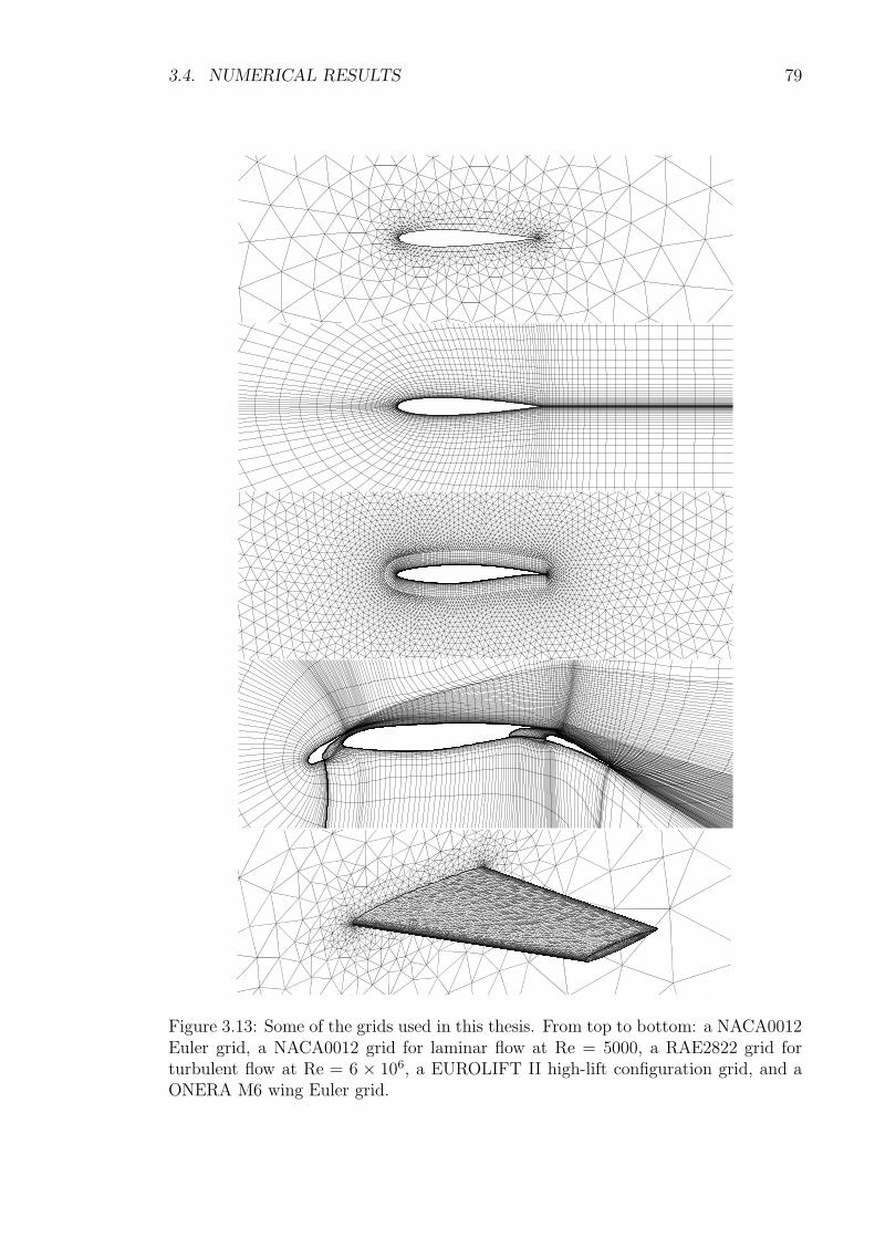
3.4. NUMERICAL RESULTS 79
Figure 3.13: Some of the grids used in this thesis. From top to bottom: a NACA0012Euler grid, a NACA0012 grid for laminar flow at Re = 5000, a RAE2822 grid forturbulent flow at Re = 6 × 10⁶, a EUROLIFT II high-lift configuration grid, and aONERA M6 wing Euler grid.
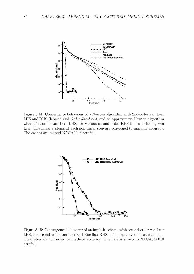
80 CHAPTER 3. APPROXIMATELY FACTORED IMPLICIT SCHEMES
Iteration
rho
resi
dual
25 50 75 100
10-13
10-11
10-9
10-7
10-5
10-3
10-1 AUSMDVAUSMPWPJSTRoeVan Leer2nd Order Jacobian
Figure 3.14: Convergence behaviour of a Newton algorithm with 2nd-order van LeerLHS and RHS (labeled 2nd-Order Jacobian), and an approximate Newton algorithmwith a 1st-order van Leer LHS, for various second-order RHS fluxes including vanLeer. The linear systems at each non-linear step are converged to machine accuracy.The case is an inviscid NACA0012 aerofoil.
Inner-iter
Res
idua
l
110 120 130 140 150
10-12
10-10
10-8
10-6
10-4
10-2
100
LHS/RHS AusmDV2LHS Roe2 RHS AusmDV2
Figure 3.15: Convergence behaviour of an implicit scheme with second-order van LeerLHS, for second-order van Leer and Roe flux RHS. The linear systems at each non-linear step are converged to machine accuracy. The case is a viscous NACA64A010aerofoil.
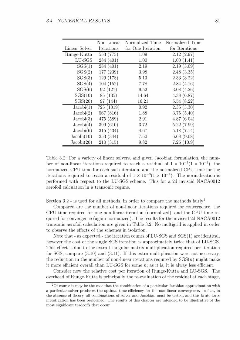
3.4. NUMERICAL RESULTS 81
Non-Linear Normalized Time Normalized TimeLinear Solver Iterations for One Iteration for IterationsRunge-Kutta 553 (775) 1.09 2.12 (2.97)
LU-SGS 284 (401) 1.00 1.00 (1.41)SGS(1) 284 (401) 2.19 2.19 (3.09)SGS(2) 177 (239) 3.98 2.48 (3.35)SGS(3) 129 (178) 5.13 2.33 (3.22)SGS(4) 104 (152) 7.78 2.84 (4.16)SGS(6) 92 (127) 9.52 3.08 (4.26)
SGS(10) 85 (135) 14.64 4.38 (6.87)SGS(20) 97 (144) 16.21 5.54 (8.22)
Jacobi(1) 725 (1019) 0.92 2.35 (3.30)Jacobi(2) 567 (816) 1.88 3.75 (5.40)Jacobi(3) 475 (589) 2.91 4.87 (6.04)Jacobi(4) 399 (610) 3.72 5.22 (7.99)Jacobi(6) 315 (434) 4.67 5.18 (7.14)
Jacobi(10) 253 (344) 7.50 6.68 (9.08)Jacobi(20) 210 (315) 9.82 7.26 (10.9)
Table 3.2: For a variety of linear solvers, and given Jacobian formulation, the num-ber of non-linear iterations required to reach a residual of 1 × 10⁻³(1 × 10⁻⁴), thenormalized CPU time for each such iteration, and the normalized CPU time for theiterations required to reach a residual of 1 × 10⁻³(1 × 10⁻⁴). The normalization isperformed with respect to the LU-SGS scheme. This for a 2d inviscid NACA0012aerofoil calcuation in a transonic regime.
Section 3.2 - is used for all methods, in order to compare the methods fairly2.Compared are the number of non-linear iterations required for convergence, the
CPU time required for one non-linear iteration (normalized), and the CPU time re-quired for convergence (again normalized). The results for the inviscid 2d NACA0012transonic aerofoil calculation are given in Table 3.2. No multigrid is applied in orderto observe the effects of the schemes in isolation.
Note that - as expected - the iteration counts of LU-SGS and SGS(1) are identical,however the cost of the single SGS iteration is approximately twice that of LU-SGS.This effect is due to the extra triangular matrix multiplication required per iterationfor SGS; compare (3.10) and (3.11). If this extra multiplication were not necessary,the reduction in the number of non-linear iterations required by SGS(n) might makeit more efficient overall than LU-SGS for some n; as it is, it is alway less efficient.
Consider now the relative cost per iteration of Runge-Kutta and LU-SGS. Theoverhead of Runge-Kutta is principally the re-evaluation of the residual at each stage,
2Of course it may be the case that the combination of a particular Jacobian approximation witha particular solver produces the optimal time-efficiency for the non-linear convergence. In fact, inthe absence of theory, all combinations of solver and Jacobian must be tested, and this brute-forceinvestigation has been performed. The results of this chapter are intended to be illustrative of themost significant tradeoffs that occur.
82 CHAPTER 3. APPROXIMATELY FACTORED IMPLICIT SCHEMES
whereas the SGS algorithms require only one evaluation of the residual for each non-linear iteration. On the other hand the SGS algorithms must compute the Jacobianand perform two Gauss-Seidel sweeps per inner iteration. If the residual is veryexpensive to compute, it will drive up the cost of Runge-Kutta, and LU-SGS will becomparatively efficient3. As it happens, the two extra residual evaluations are moreexpensive than the LU-SGS overhead, and hence LU-SGS is more efficient per step.Here the cheapest available flux is used (the JST flux), and hence the difference inCPU time per step is relatively small; for matrix dissipation with preconditioningLU-SGS is considerably faster per step than Runge-Kutta.
Jacobi(1) is slightly cheaper than LU-SGS, but Jacobi has poorer convergencebehaviour than Gauss-Seidel and the CFL condition limits the time step. Jacobi(2)is already twice as expensive as LU-SGS, but to get the same convergence behaviourwith Jacobi, between 6 and 10 inner steps are required, at which point the expenseper step is prohibitive.
The reason that Jacobi iterations perform so poorly for this case is that thediagonal-blocks of the Jacobian are simply multiples of the identity matrix, and henceone step of (3.14) is equivalent to a forward-Euler method with a local time step.In constrast, Jacobi iterations have been shown to be effective when applied to aspatial discretization with matrix dissipation (Swanson et al., 2005; Mavriplis, 1998;Pierce et al., 1997), where the coefficient of the dissipative fluxes contains the matrix|∂f c/∂W | rather than simply the maximum eigenvalue thereof. In this case thediagonal-block of the Jacobian contains significantly more flow information, and asmight be expected the method is therefore superior4. The use of such Jacobians withscalar dissipation is however ineffective due to the mismatch between the residual andJacobian.
In conclusion LU-SGS is at least twice as efficient as the next best method testedfor the given Jacobian and the central discretization with scalar dissipation.
3.4.3 Influence of Viscous Flux Approximation
Three formulations of the viscous TSL Jacobian proposed in Section 3.2.3 are numer-ically compared, from most accurate to least accurate they are:
Exact TSL No approximations are made, the TSL block Jacobian contributions areexactly those given in Section 2.8.1.
Diagonalized Diagonal The TSL block Jacobians that occur on the diagonal arereplaced by the sum of their spectral radii, thus diagonalizing the block diagonalas described in Section 3.2.3.
Fully Diagonalized All TSL block Jacobians occurring in the system matrix arereplaced by their spectral radii, thus removing all coupling of the equations overthe viscous terms.
3Runge-Kutta has here the advantage that the dissipation in the JST scheme is only calculatedon the first stage.
4This method is also known as matrix-preconditioning in reference to local time stepping as atype of scalar preconditioning.
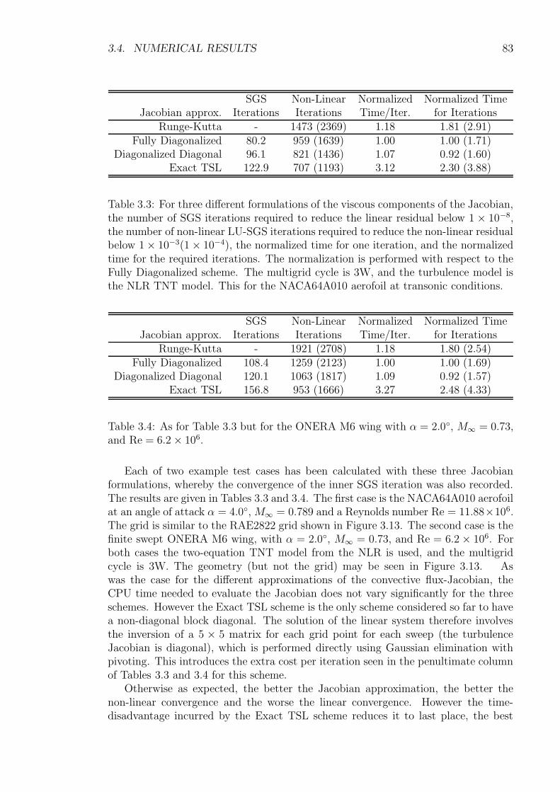
3.4. NUMERICAL RESULTS 83
SGS Non-Linear Normalized Normalized TimeJacobian approx. Iterations Iterations Time/Iter. for Iterations
Runge-Kutta - 1473 (2369) 1.18 1.81 (2.91)Fully Diagonalized 80.2 959 (1639) 1.00 1.00 (1.71)
Diagonalized Diagonal 96.1 821 (1436) 1.07 0.92 (1.60)Exact TSL 122.9 707 (1193) 3.12 2.30 (3.88)
Table 3.3: For three different formulations of the viscous components of the Jacobian,the number of SGS iterations required to reduce the linear residual below 1 × 10⁻⁸,the number of non-linear LU-SGS iterations required to reduce the non-linear residualbelow 1× 10⁻³(1× 10⁻⁴), the normalized time for one iteration, and the normalizedtime for the required iterations. The normalization is performed with respect to theFully Diagonalized scheme. The multigrid cycle is 3W, and the turbulence model isthe NLR TNT model. This for the NACA64A010 aerofoil at transonic conditions.
SGS Non-Linear Normalized Normalized TimeJacobian approx. Iterations Iterations Time/Iter. for Iterations
Runge-Kutta - 1921 (2708) 1.18 1.80 (2.54)Fully Diagonalized 108.4 1259 (2123) 1.00 1.00 (1.69)
Diagonalized Diagonal 120.1 1063 (1817) 1.09 0.92 (1.57)Exact TSL 156.8 953 (1666) 3.27 2.48 (4.33)
Table 3.4: As for Table 3.3 but for the ONERA M6 wing with α = 2.0, M∞ = 0.73,and Re = 6.2× 10⁶.
Each of two example test cases has been calculated with these three Jacobianformulations, whereby the convergence of the inner SGS iteration was also recorded.The results are given in Tables 3.3 and 3.4. The first case is the NACA64A010 aerofoilat an angle of attack α = 4.0, M∞ = 0.789 and a Reynolds number Re = 11.88×10⁶.The grid is similar to the RAE2822 grid shown in Figure 3.13. The second case is thefinite swept ONERA M6 wing, with α = 2.0, M∞ = 0.73, and Re = 6.2× 10⁶. Forboth cases the two-equation TNT model from the NLR is used, and the multigridcycle is 3W. The geometry (but not the grid) may be seen in Figure 3.13. Aswas the case for the different approximations of the convective flux-Jacobian, theCPU time needed to evaluate the Jacobian does not vary significantly for the threeschemes. However the Exact TSL scheme is the only scheme considered so far to havea non-diagonal block diagonal. The solution of the linear system therefore involvesthe inversion of a 5 × 5 matrix for each grid point for each sweep (the turbulenceJacobian is diagonal), which is performed directly using Gaussian elimination withpivoting. This introduces the extra cost per iteration seen in the penultimate columnof Tables 3.3 and 3.4 for this scheme.
Otherwise as expected, the better the Jacobian approximation, the better thenon-linear convergence and the worse the linear convergence. However the time-disadvantage incurred by the Exact TSL scheme reduces it to last place, the best
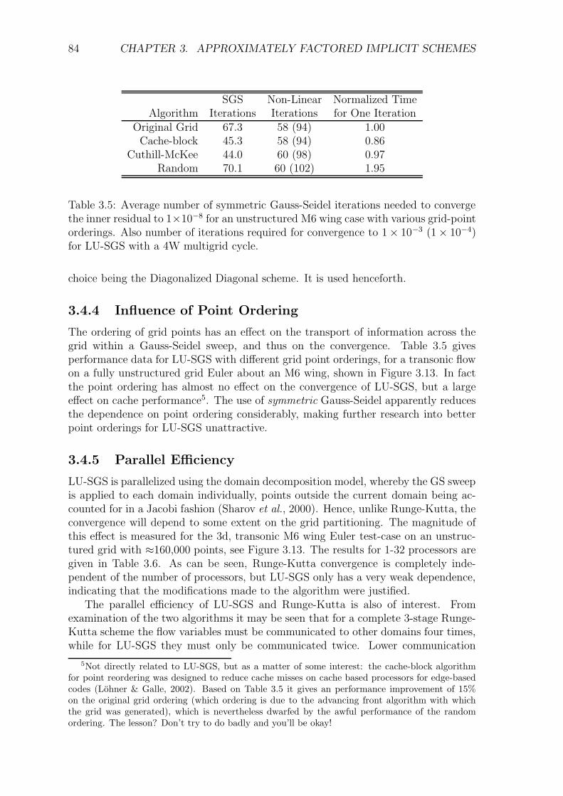
84 CHAPTER 3. APPROXIMATELY FACTORED IMPLICIT SCHEMES
SGS Non-Linear Normalized TimeAlgorithm Iterations Iterations for One Iteration
Original Grid 67.3 58 (94) 1.00Cache-block 45.3 58 (94) 0.86
Cuthill-McKee 44.0 60 (98) 0.97Random 70.1 60 (102) 1.95
Table 3.5: Average number of symmetric Gauss-Seidel iterations needed to convergethe inner residual to 1×10⁻⁸ for an unstructured M6 wing case with various grid-pointorderings. Also number of iterations required for convergence to 1× 10⁻³ (1× 10⁻⁴)for LU-SGS with a 4W multigrid cycle.
choice being the Diagonalized Diagonal scheme. It is used henceforth.
3.4.4 Influence of Point Ordering
The ordering of grid points has an effect on the transport of information across thegrid within a Gauss-Seidel sweep, and thus on the convergence. Table 3.5 givesperformance data for LU-SGS with different grid point orderings, for a transonic flowon a fully unstructured grid Euler about an M6 wing, shown in Figure 3.13. In factthe point ordering has almost no effect on the convergence of LU-SGS, but a largeeffect on cache performance5. The use of symmetric Gauss-Seidel apparently reducesthe dependence on point ordering considerably, making further research into betterpoint orderings for LU-SGS unattractive.
3.4.5 Parallel Efficiency
LU-SGS is parallelized using the domain decomposition model, whereby the GS sweepis applied to each domain individually, points outside the current domain being ac-counted for in a Jacobi fashion (Sharov et al., 2000). Hence, unlike Runge-Kutta, theconvergence will depend to some extent on the grid partitioning. The magnitude ofthis effect is measured for the 3d, transonic M6 wing Euler test-case on an unstruc-tured grid with ≈160,000 points, see Figure 3.13. The results for 1-32 processors aregiven in Table 3.6. As can be seen, Runge-Kutta convergence is completely inde-pendent of the number of processors, but LU-SGS only has a very weak dependence,indicating that the modifications made to the algorithm were justified.
The parallel efficiency of LU-SGS and Runge-Kutta is also of interest. Fromexamination of the two algorithms it may be seen that for a complete 3-stage Runge-Kutta scheme the flow variables must be communicated to other domains four times,while for LU-SGS they must only be communicated twice. Lower communication
5Not directly related to LU-SGS, but as a matter of some interest: the cache-block algorithmfor point reordering was designed to reduce cache misses on cache based processors for edge-basedcodes (Lohner & Galle, 2002). Based on Table 3.5 it gives an performance improvement of 15%on the original grid ordering (which ordering is due to the advancing front algorithm with whichthe grid was generated), which is nevertheless dwarfed by the awful performance of the randomordering. The lesson? Don’t try to do badly and you’ll be okay!
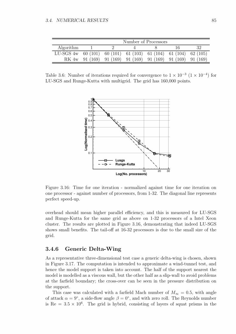
3.4. NUMERICAL RESULTS 85
Number of ProcessorsAlgorithm 1 2 4 8 16 32
LU-SGS 4w 60 (101) 60 (101) 61 (103) 61 (104) 61 (104) 62 (105)RK 4w 91 (169) 91 (169) 91 (169) 91 (169) 91 (169) 91 (169)
Table 3.6: Number of iterations required for convergence to 1 × 10⁻³ (1× 10⁻⁴) forLU-SGS and Runge-Kutta with multigrid. The grid has 160,000 points.
Log(No. processors)
Log(
Nor
mal
ised
time)
10 20 30
0.1
0.2
0.3
0.4
0.5
0.60.70.80.9
1
LusgsRunge-Kutta
Figure 3.16: Time for one iteration - normalized against time for one iteration onone processor - against number of processors, from 1-32. The diagonal line representsperfect speed-up.
overhead should mean higher parallel efficiency, and this is measured for LU-SGSand Runge-Kutta for the same grid as above on 1-32 processors of a Intel Xeoncluster. The results are plotted in Figure 3.16, demonstrating that indeed LU-SGSshows small benefits. The tail-off at 16-32 processors is due to the small size of thegrid.
3.4.6 Generic Delta-Wing
As a representative three-dimensional test case a generic delta-wing is chosen, shownin Figure 3.17. The computation is intended to approximate a wind-tunnel test, andhence the model support is taken into account. The half of the support nearest themodel is modelled as a viscous wall, but the other half as a slip-wall to avoid problemsat the farfield boundary; the cross-over can be seen in the pressure distribution onthe support.
This case was calculated with a farfield Mach number of M∞ = 0.5, with angleof attack α = 9, a side-flow angle β = 0, and with zero roll. The Reynolds numberis Re = 3.5 × 10⁶. The grid is hybrid, consisting of layers of squat prisms in the
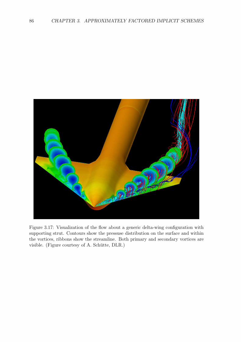
86 CHAPTER 3. APPROXIMATELY FACTORED IMPLICIT SCHEMES
Figure 3.17: Visualization of the flow about a generic delta-wing configuration withsupporting strut. Contours show the pressuse distribution on the surface and withinthe vortices, ribbons show the streamline. Both primary and secondary vortices arevisible. (Figure courtesy of A. Schutte, DLR.)
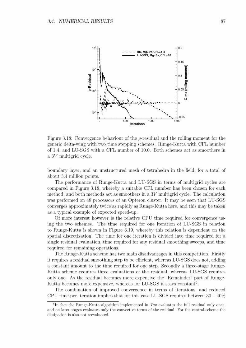
3.4. NUMERICAL RESULTS 87
Iterations
ρ-R
esid
ual
C-m
x(r
ollin
gm
omen
t)
0 500 1000 1500
10-3
10-2
10-1
100
-0.05
0
0.05
0.1
0.15
0.2RK, Mg=3v, CFL=1.4LU-SGS, Mg=3v, CFL=10
Figure 3.18: Convergence behaviour of the ρ-residual and the rolling moment for thegeneric delta-wing with two time stepping schemes: Runge-Kutta with CFL numberof 1.4, and LU-SGS with a CFL number of 10.0. Both schemes act as smoothers ina 3V multigrid cycle.
boundary layer, and an unstructured mesh of tetrahedra in the field, for a total ofabout 3.4 million points.
The performance of Runge-Kutta and LU-SGS in terms of multigrid cycles arecompared in Figure 3.18, whereby a suitable CFL number has been chosen for eachmethod, and both methods act as smoothers in a 3V multigrid cycle. The calculationwas performed on 48 processors of an Opteron cluster. It may be seen that LU-SGSconverges approximately twice as rapidly as Runge-Kutta here, and this may be takenas a typical example of expected speed-up.
Of more interest however is the relative CPU time required for convergence us-ing the two schemes. The time required for one iteration of LU-SGS in relationto Runge-Kutta is shown in Figure 3.19, whereby this relation is dependent on thespatial discretization. The time for one iteration is divided into time required for asingle residual evaluation, time required for any residual smoothing sweeps, and timerequired for remaining operations.
The Runge-Kutta scheme has two main disadvantages in this competition. Firstlyit requires a residual smoothing step to be efficient, whereas LU-SGS does not, addinga constant amount to the time required for one step. Secondly a three-stage Runge-Kutta scheme requires three evaluations of the residual, whereas LU-SGS requiresonly one. As the residual becomes more expensive the “Remainder” part of Runge-Kutta becomes more expensive, whereas for LU-SGS it stays constant6.
The combination of improved convergence in terms of iterations, and reducedCPU time per iteration implies that for this case LU-SGS requires between 30− 40%
6In fact the Runge-Kutta algorithm implemented in Tau evaluates the full residual only once,and on later stages evaluates only the convective terms of the residual. For the central scheme thedissipation is also not reevaluated.
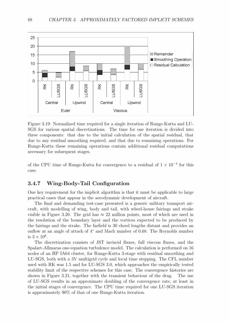
88 CHAPTER 3. APPROXIMATELY FACTORED IMPLICIT SCHEMES
Figure 3.19: Normalized time required for a single iteration of Runge-Kutta and LU-SGS for various spatial discretizations. The time for one iteration is divided intothree components: that due to the initial calculation of the spatial residual, thatdue to any residual smoothing required, and that due to remaining operations. ForRunge-Kutta these remaining operations contain additional residual computationsnecessary for subsequent stages.
of the CPU time of Runge-Kutta for convergence to a residual of 1 × 10⁻⁴ for thiscase.
3.4.7 Wing-Body-Tail Configuration
One key requirement for the implicit algorithm is that it must be applicable to largepractical cases that appear in the aerodynamic development of aircraft.
The final and demanding test-case presented is a generic military transport air-craft, with modelling of wing, body and tail, with wheel-house fairings and strakevisible in Figure 3.20. The grid has ≈ 22 million points, most of which are used inthe resolution of the boundary layer and the vortices expected to be produced bythe fairings and the strake. The farfield is 30 chord lengths distant and provides anonflow at an angle of attack of 4 and Mach number of 0.68. The Reynolds numberis 3× 10⁶.
The discretization consists of JST inviscid fluxes, full viscous fluxes, and theSpalart-Allmaras one-equation turbulence model. The calculation is performed on 16nodes of an HP IA64 cluster, for Runge-Kutta 3-stage with residual smoothing andLU-SGS, both with a 3V multigrid cycle and local time stepping. The CFL numberused with RK was 1.5 and for LU-SGS 3.0, which approaches the empirically testedstability limit of the respective schemes for this case. The convergence histories areshown in Figure 3.21, together with the transient behaviour of the drag. The useof LU-SGS results in an approximate doubling of the convergence rate, at least inthe initial stages of convergence. The CPU time required for one LU-SGS iterationis approximately 90% of that of one Runge-Kutta iteration.
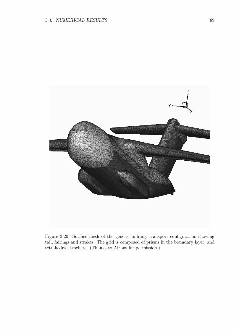
3.4. NUMERICAL RESULTS 89
Figure 3.20: Surface mesh of the generic military transport configuration showingtail, fairings and strakes. The grid is composed of prisms in the boundary layer, andtetrahedra elsewhere. (Thanks to Airbus for permission.)
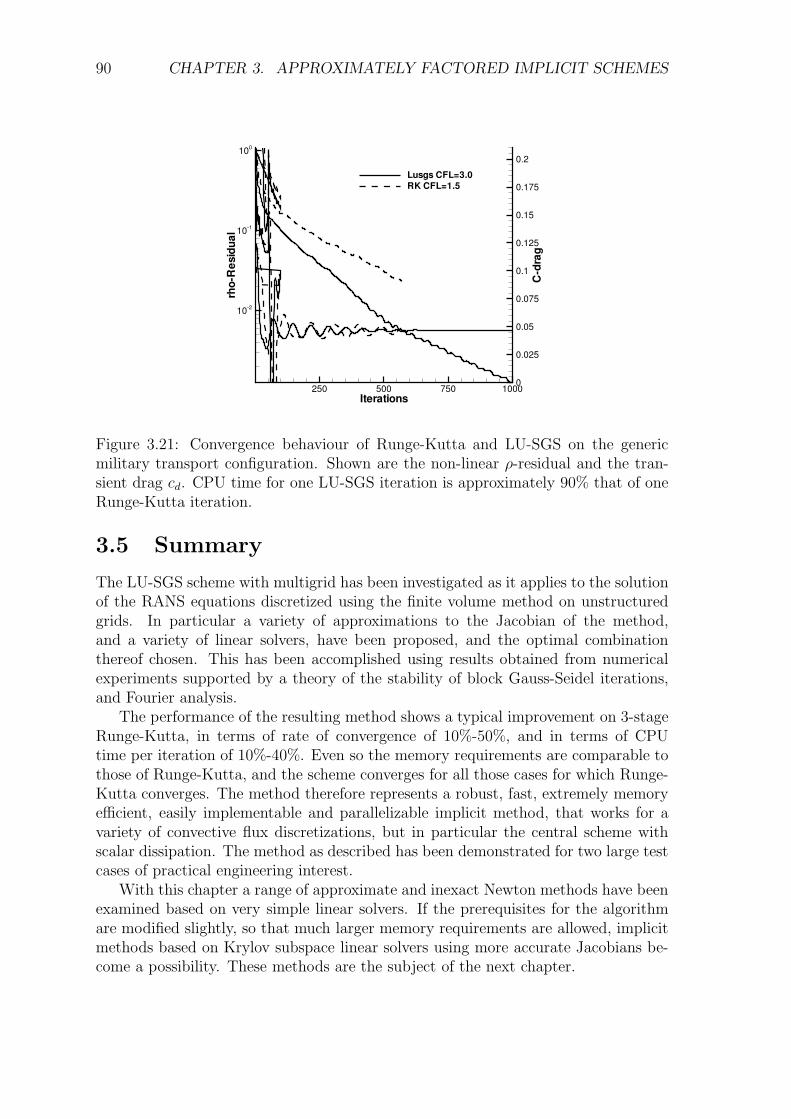
90 CHAPTER 3. APPROXIMATELY FACTORED IMPLICIT SCHEMES
Iterations
rho-
Res
idua
l
C-d
rag
250 500 750 1000
10-2
10-1
100
0
0.025
0.05
0.075
0.1
0.125
0.15
0.175
0.2
Lusgs CFL=3.0RK CFL=1.5
Figure 3.21: Convergence behaviour of Runge-Kutta and LU-SGS on the genericmilitary transport configuration. Shown are the non-linear ρ-residual and the tran-sient drag cd. CPU time for one LU-SGS iteration is approximately 90% that of oneRunge-Kutta iteration.
3.5 Summary
The LU-SGS scheme with multigrid has been investigated as it applies to the solutionof the RANS equations discretized using the finite volume method on unstructuredgrids. In particular a variety of approximations to the Jacobian of the method,and a variety of linear solvers, have been proposed, and the optimal combinationthereof chosen. This has been accomplished using results obtained from numericalexperiments supported by a theory of the stability of block Gauss-Seidel iterations,and Fourier analysis.
The performance of the resulting method shows a typical improvement on 3-stageRunge-Kutta, in terms of rate of convergence of 10%-50%, and in terms of CPUtime per iteration of 10%-40%. Even so the memory requirements are comparable tothose of Runge-Kutta, and the scheme converges for all those cases for which Runge-Kutta converges. The method therefore represents a robust, fast, extremely memoryefficient, easily implementable and parallelizable implicit method, that works for avariety of convective flux discretizations, but in particular the central scheme withscalar dissipation. The method as described has been demonstrated for two large testcases of practical engineering interest.
With this chapter a range of approximate and inexact Newton methods have beenexamined based on very simple linear solvers. If the prerequisites for the algorithmare modified slightly, so that much larger memory requirements are allowed, implicitmethods based on Krylov subspace linear solvers using more accurate Jacobians be-come a possibility. These methods are the subject of the next chapter.
Chapter 4
Unfactored Implicit Schemes
4.1 Introduction
The philosophy of the development of the implicit scheme of Chapter 3 was that sucha scheme could be an effective alternative to an explicit Runge-Kutta method forlarge applications in aerospace engineering, if it had similar memory requirements,no start-up difficulties, and could be easily parallelized. This was achieved with theLU-SGS scheme, whereby these restrictions (in particular the first) severely limitedthe choice of Jacobian, and hence the convergence rate possible.
In this chapter these restrictions are relaxed, and schemes are considered thatmay have significantly larger memory requirements than explicit methods. This maybe justified by noting that for the cluster computers which increasingly dominate thescientific computing landscape, and which typically have large amounts of memoryper node, the limiting factor in common engineering applications is cluster CPUtime. For a given case and an efficient parallel solver, the total CPU time neededis roughly a constant function of the number of processors used; however the wall-clock time falls in inverse proportion to the number of processors. Engineers requiretimely results and so use many processors, whereby the full memory capacity of theindividual nodes often remains unused. An implicit method, even with significantlylarger memory requirements, would be practical under such conditions, provided thatit is efficient in parallel. This is not to say that memory considerations may be ignoredaltogether however, and efforts will be made to produce a memory-efficient method.
Another disadvantage of LU-SGS was that because the implicit operator developedwas not accurate enough to provide effective full-domain communication within oneiteration on its own, the method was only efficient when used as a multigrid smoother(this is not the case for an exact Newton method, for example). While multigrid onstructured grids is extremely effective (Pierce et al., 1997), on unstructured gridsit often suffers under poor coarse-grid quality, due to the difficulty of producing acell agglomeration algorithm that results in smooth convex volumes in 3D. Someselected coarse grid cells from the second multigrid level of a 3d calculation usingthe TAU-code are shown in Fig. 4.1; note that even on the surface the volumes areirregular, while in the field there is even a cell shaped like a banana. The influence ofthe multigrid correction in this region of the mesh was shown to cause divergence ofthe entire calculation in this case. One aim of the development of implicit methods inthis chapter is therefore the removal of non-linear multigrid from the solution process,
91
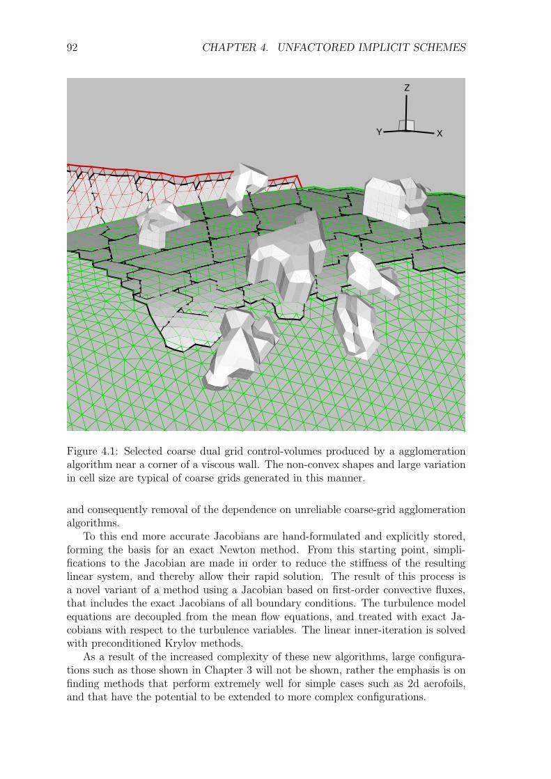
92 CHAPTER 4. UNFACTORED IMPLICIT SCHEMES
XY
Z
Figure 4.1: Selected coarse dual grid control-volumes produced by a agglomerationalgorithm near a corner of a viscous wall. The non-convex shapes and large variationin cell size are typical of coarse grids generated in this manner.
and consequently removal of the dependence on unreliable coarse-grid agglomerationalgorithms.
To this end more accurate Jacobians are hand-formulated and explicitly stored,forming the basis for an exact Newton method. From this starting point, simpli-fications to the Jacobian are made in order to reduce the stiffness of the resultinglinear system, and thereby allow their rapid solution. The result of this process isa novel variant of a method using a Jacobian based on first-order convective fluxes,that includes the exact Jacobians of all boundary conditions. The turbulence modelequations are decoupled from the mean flow equations, and treated with exact Ja-cobians with respect to the turbulence variables. The linear inner-iteration is solvedwith preconditioned Krylov methods.
As a result of the increased complexity of these new algorithms, large configura-tions such as those shown in Chapter 3 will not be shown, rather the emphasis is onfinding methods that perform extremely well for simple cases such as 2d aerofoils,and that have the potential to be extended to more complex configurations.
4.1. INTRODUCTION 93
4.1.1 Overview
This chapter begins with a general description of the methods used for the per-handimplementation and verification of the Jacobian of the finite volume discretization ofTAU, see Section 4.2. The Jacobian is exact in the sense that each and every compo-nent of R(W ) is differentiated exactly, including boundary conditions and turbulencemodels, with no simplifications or approximations made. The techniques describedare applicable to the differentiation of flow solvers in general.
Corresponding to the stiffness of the non-linear problem the Jacobian is verypoorly conditioned, especially for Navier-Stokes problems. Section 4.3 examines thesolution of linear systems involving the exact Jacobian, and considers preconditionedKrylov algorithms. In particular Incomplete Lower-Upper (ILU) preconditioned Gen-eralized Minimal Residual Method (GMRES) is examined, and it is seen that fortimely convergence very large ILU fill-in levels are required, having correspondinglylarge memory requirements. It is also seen, as previously reported (Campobasso &Giles, 2002), that for linear systems resulting from Newton iterations based on par-tially converged non-linear solutions, a necessary condition for convergence of Jacobior Gauss-Seidel iterations on the linear system is not satisfied. In this situation aKrylov solver is essential, and Jacobi and Gauss-Seidel are poor preconditioners.
Using ILU preconditioned GMRES and an explicitly stored Jacobian, an exactNewton method is constructed and tested on a turbulent RAE2822 test case. Quadra-tic convergence is observed, and the method is much faster than LU-SGS, but requiresILU(4) preconditioning and may only be started after five orders of magnitude re-duction in the residual have been achieved.
Given these significant difficulties with exact Newton methods, attention is againturned to approximate Newton methods. Section 4.5 considers a method based onan explicitly stored, first-order Jacobian. As the reduction to first-order is morenatural for upwind schemes, the investigation begins with an implicit method forRoe’s scheme. This is briefly compared with another recently proposed and similarmethod, also for Roe (Rossow, 2005). However the goal is to improve performanceusing the JST scheme as the spatial discretization. Hence a first-order JST Jacobianis proposed and solved with ILU preconditioned GMRES. The method is shown tobe 4-5 times faster than the LU-SGS method for the cases considered, has no relianceon geometric multigrid, and may be easily parallelized.
Throughout this chapter the RAE2822 Test-Case Definitions 9 and 10 will beused, which have come to be standard reference cases in CFD, in particular in thearea of turbulence modelling. They are defined in (Cook et al., 1979) along withdetailed experimental results. Both cases are transonic flows about the non-symmetricRAE2822 single element aerofoil, with chord Reynolds numbers of 6.5 × 10⁶ and6.2× 106, at Mach numbers of 0.73 and 0.75 respectively. The angle-of-attack is 2.8.Both cases are transonic with normal shocks on the aerofoil upper surface. Case 9is fully attached, while Case 10 has a small area of separated flow near the trailingedge. The grid used is shown in Figure 3.13 and has about 14× 103 points.
94 CHAPTER 4. UNFACTORED IMPLICIT SCHEMES
4.2 Construction of the Exact Jacobian
Implementation of an exact Newton method requires the ability to formulate andsolve linear systems of the form
∂R
∂W∆W = −R(W ),
with respect to ∆W . The residual R is taken to be readily available here, whereasthe Jacobian ∂R/∂W may be difficult to obtain.
One option is to use finite differences to approximate the Jacobian-vector product,and use solution algorithms that require only this product, and not the Jacobianexplicitly. This was examined briefly in Section 3.4.1, and was found not to becompetitive with LU-SGS because of the expense of repeated evaluations of R. Itmay be the case that an alternative Krylov solver/preconditioner combination wouldrequire less Jacobian-vector products, but a more promising alternative is to use anexplicitly stored Jacobian.
The Jacobian may be evaluated by hand, which is a straightforward exercise asR may be written explicitly in terms of W , while being very time-consuming asR is typically extremely complex, as illustrated in Section 2.6.3. However, as R isa sum of convective fluxes, viscous fluxes, boundary conditions etc., each of thesemay be differentiated independently, and may be further subdivided into manageablechunks by application of the chain rule. The operation of differentiation is furthersimplified by choosing primitive variables as working variables. Because the equationsthemselves remain in conservative form, this choice has no effect on the final solution,however the update ∆W will then be in terms of primitive variables. Strong boundaryconditions such as the specification of zero velocity on viscous walls are handled asdiscussed in Section 2.9.4.
The accuracy of the implementation of the derivatives of the individual fluxes isverified by applying finite differences to the original routines, and comparing with thehand-calculated Jacobian for a variety of inputs. As each flux derivative is calculated,a contribution is made to the explicitly stored Jacobian.
To provide an insight into the implementation, the somewhat personal processdeveloped by the author after much trial and error is offered here, in the hope that itmay guide initial efforts of others. It may be summarized in the following six steps:
1. Divide the code for the non-linear residual R into parts that may be differen-tiated independently - either because R is a simple sum of e.g. inviscid andviscous fluxes, or by means of the product and chain rules. All parts of thecode that do not influence the solution of R(W ) = 0, are superfluous.
2. Copy out the definition for e.g. a particular flux function f , directly from thecode onto paper. Begin with the definition of f in terms of intermediate vari-ables at the end of the code fragment, and proceed upwards. This order will aidthe application of the chain rule in Step 4. In order that the resulting Jacobianbe the exact derivative of R it is the author’s experience that it is not sufficientto take flux function definitions from technical reports, published articles etc.,as the reality is often substantially different.
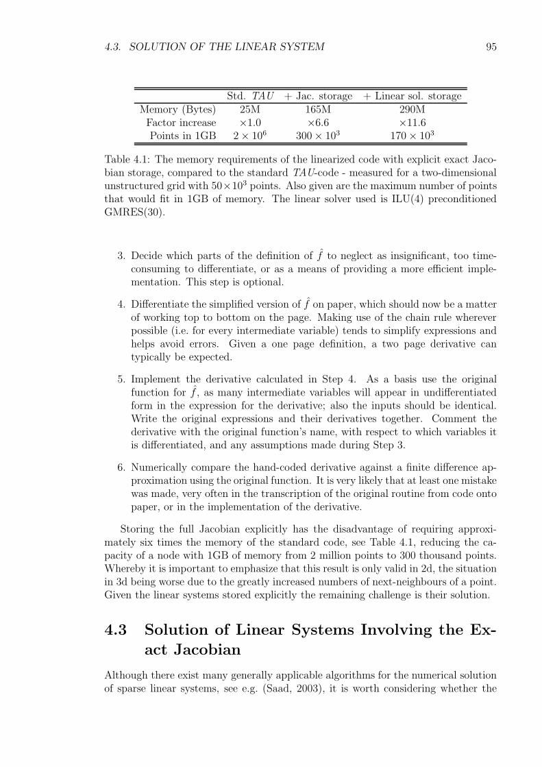
4.3. SOLUTION OF THE LINEAR SYSTEM 95
Std. TAU + Jac. storage + Linear sol. storageMemory (Bytes) 25M 165M 290M
Factor increase ×1.0 ×6.6 ×11.6Points in 1GB 2× 10⁶ 300× 103 170× 103
Table 4.1: The memory requirements of the linearized code with explicit exact Jaco-bian storage, compared to the standard TAU-code - measured for a two-dimensionalunstructured grid with 50×103 points. Also given are the maximum number of pointsthat would fit in 1GB of memory. The linear solver used is ILU(4) preconditionedGMRES(30).
3. Decide which parts of the definition of f to neglect as insignificant, too time-consuming to differentiate, or as a means of providing a more efficient imple-mentation. This step is optional.
4. Differentiate the simplified version of f on paper, which should now be a matterof working top to bottom on the page. Making use of the chain rule whereverpossible (i.e. for every intermediate variable) tends to simplify expressions andhelps avoid errors. Given a one page definition, a two page derivative cantypically be expected.
5. Implement the derivative calculated in Step 4. As a basis use the originalfunction for f , as many intermediate variables will appear in undifferentiatedform in the expression for the derivative; also the inputs should be identical.Write the original expressions and their derivatives together. Comment thederivative with the original function’s name, with respect to which variables itis differentiated, and any assumptions made during Step 3.
6. Numerically compare the hand-coded derivative against a finite difference ap-proximation using the original function. It is very likely that at least one mistakewas made, very often in the transcription of the original routine from code ontopaper, or in the implementation of the derivative.
Storing the full Jacobian explicitly has the disadvantage of requiring approxi-mately six times the memory of the standard code, see Table 4.1, reducing the ca-pacity of a node with 1GB of memory from 2 million points to 300 thousand points.Whereby it is important to emphasize that this result is only valid in 2d, the situationin 3d being worse due to the greatly increased numbers of next-neighbours of a point.Given the linear systems stored explicitly the remaining challenge is their solution.
4.3 Solution of Linear Systems Involving the Ex-
act Jacobian
Although there exist many generally applicable algorithms for the numerical solutionof sparse linear systems, see e.g. (Saad, 2003), it is worth considering whether the
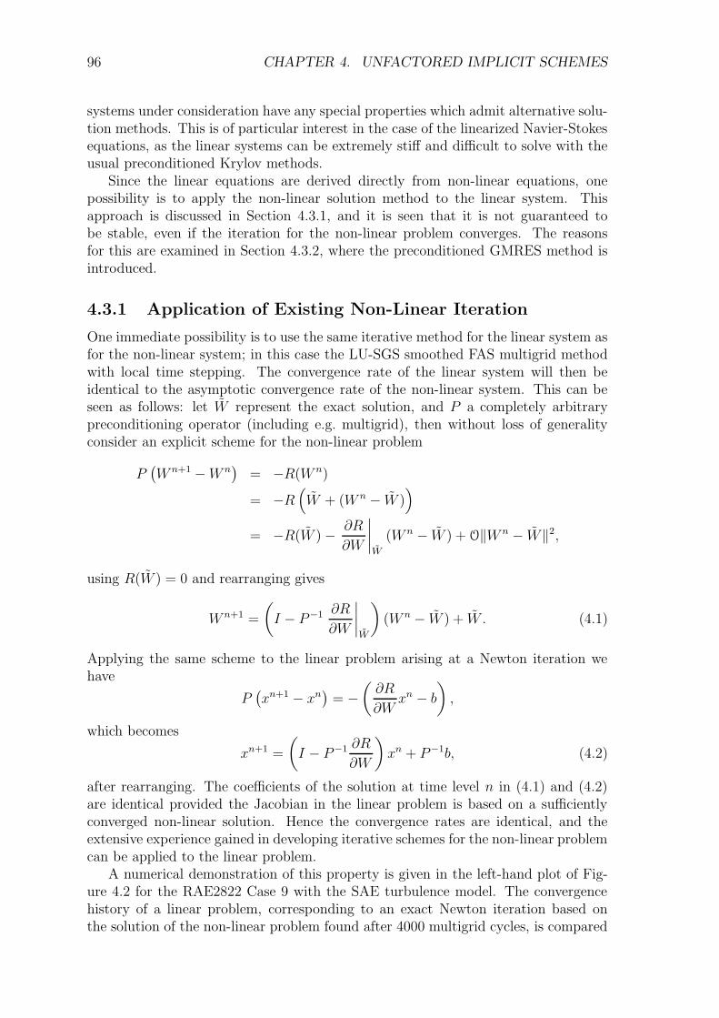
96 CHAPTER 4. UNFACTORED IMPLICIT SCHEMES
systems under consideration have any special properties which admit alternative solu-tion methods. This is of particular interest in the case of the linearized Navier-Stokesequations, as the linear systems can be extremely stiff and difficult to solve with theusual preconditioned Krylov methods.
Since the linear equations are derived directly from non-linear equations, onepossibility is to apply the non-linear solution method to the linear system. Thisapproach is discussed in Section 4.3.1, and it is seen that it is not guaranteed tobe stable, even if the iteration for the non-linear problem converges. The reasonsfor this are examined in Section 4.3.2, where the preconditioned GMRES method isintroduced.
4.3.1 Application of Existing Non-Linear Iteration
One immediate possibility is to use the same iterative method for the linear system asfor the non-linear system; in this case the LU-SGS smoothed FAS multigrid methodwith local time stepping. The convergence rate of the linear system will then beidentical to the asymptotic convergence rate of the non-linear system. This can beseen as follows: let W represent the exact solution, and P a completely arbitrarypreconditioning operator (including e.g. multigrid), then without loss of generalityconsider an explicit scheme for the non-linear problem
P(W n+1 −W n
)= −R(W n)
= −R(W + (W n − W )
)
= −R(W )− ∂R
∂W
∣∣∣∣W
(W n − W ) + O‖W n − W‖2,
using R(W ) = 0 and rearranging gives
W n+1 =
(I − P−1 ∂R
∂W
∣∣∣∣W
)(W n − W ) + W . (4.1)
Applying the same scheme to the linear problem arising at a Newton iteration wehave
P(xn+1 − xn
)= −
(∂R
∂Wxn − b
),
which becomes
xn+1 =
(I − P−1 ∂R
∂W
)xn + P−1b, (4.2)
after rearranging. The coefficients of the solution at time level n in (4.1) and (4.2)are identical provided the Jacobian in the linear problem is based on a sufficientlyconverged non-linear solution. Hence the convergence rates are identical, and theextensive experience gained in developing iterative schemes for the non-linear problemcan be applied to the linear problem.
A numerical demonstration of this property is given in the left-hand plot of Fig-ure 4.2 for the RAE2822 Case 9 with the SAE turbulence model. The convergencehistory of a linear problem, corresponding to an exact Newton iteration based onthe solution of the non-linear problem found after 4000 multigrid cycles, is compared
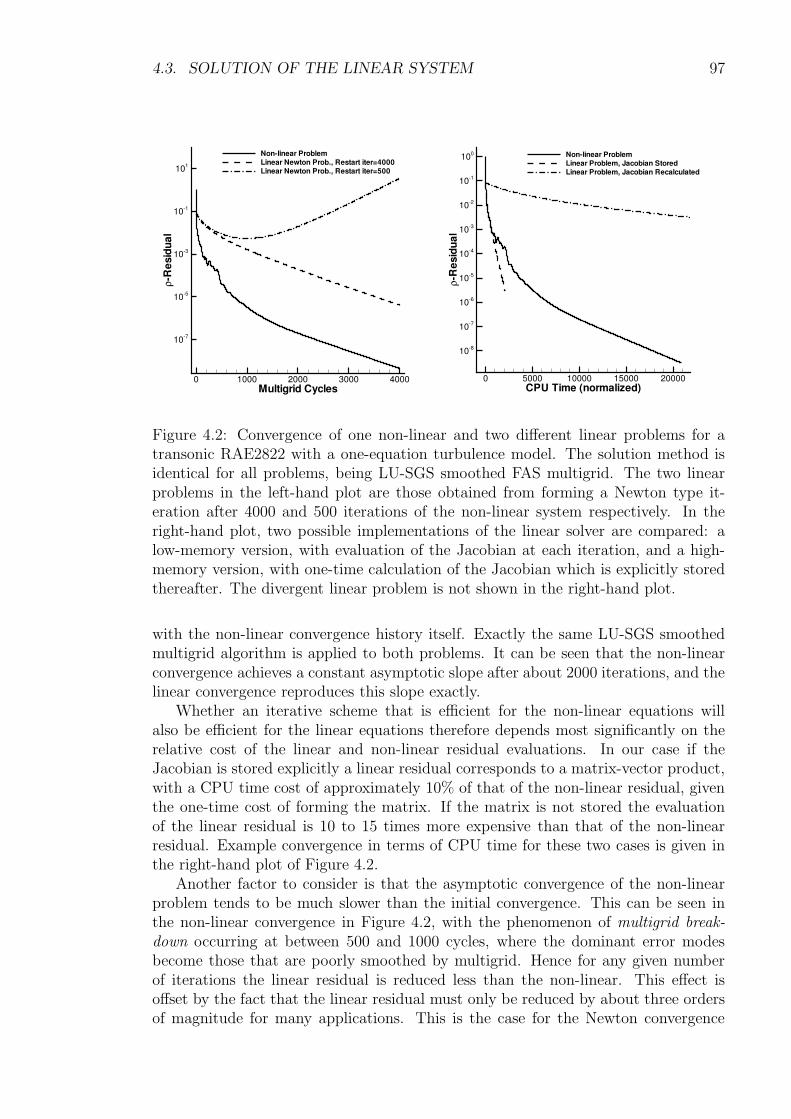
4.3. SOLUTION OF THE LINEAR SYSTEM 97
CPU Time (normalized)
ρ-R
esid
ual
0 5000 10000 15000 20000
10-8
10-7
10-6
10-5
10-4
10-3
10-2
10-1
100 Non-linear ProblemLinear Problem, Jacobian StoredLinear Problem, Jacobian Recalculated
Multigrid Cycles
ρ-R
esid
ual
0 1000 2000 3000 4000
10-7
10-5
10-3
10-1
101
Non-linear ProblemLinear Newton Prob., Restart iter=4000Linear Newton Prob., Restart iter=500
Figure 4.2: Convergence of one non-linear and two different linear problems for atransonic RAE2822 with a one-equation turbulence model. The solution method isidentical for all problems, being LU-SGS smoothed FAS multigrid. The two linearproblems in the left-hand plot are those obtained from forming a Newton type it-eration after 4000 and 500 iterations of the non-linear system respectively. In theright-hand plot, two possible implementations of the linear solver are compared: alow-memory version, with evaluation of the Jacobian at each iteration, and a high-memory version, with one-time calculation of the Jacobian which is explicitly storedthereafter. The divergent linear problem is not shown in the right-hand plot.
with the non-linear convergence history itself. Exactly the same LU-SGS smoothedmultigrid algorithm is applied to both problems. It can be seen that the non-linearconvergence achieves a constant asymptotic slope after about 2000 iterations, and thelinear convergence reproduces this slope exactly.
Whether an iterative scheme that is efficient for the non-linear equations willalso be efficient for the linear equations therefore depends most significantly on therelative cost of the linear and non-linear residual evaluations. In our case if theJacobian is stored explicitly a linear residual corresponds to a matrix-vector product,with a CPU time cost of approximately 10% of that of the non-linear residual, giventhe one-time cost of forming the matrix. If the matrix is not stored the evaluationof the linear residual is 10 to 15 times more expensive than that of the non-linearresidual. Example convergence in terms of CPU time for these two cases is given inthe right-hand plot of Figure 4.2.
Another factor to consider is that the asymptotic convergence of the non-linearproblem tends to be much slower than the initial convergence. This can be seen inthe non-linear convergence in Figure 4.2, with the phenomenon of multigrid break-down occurring at between 500 and 1000 cycles, where the dominant error modesbecome those that are poorly smoothed by multigrid. Hence for any given numberof iterations the linear residual is reduced less than the non-linear. This effect isoffset by the fact that the linear residual must only be reduced by about three ordersof magnitude for many applications. This is the case for the Newton convergence
98 CHAPTER 4. UNFACTORED IMPLICIT SCHEMES
shown in Section 4.4, as well as for the adjoint problems in the following chapter.One additional disadvantage associated with this approach is that if the convergencerate of the adjoint iteration is to be guaranteed to be the same as the non-linear thesolution procedure must be additionally adjointed. For LU-SGS or Runge-Kutta withmultigrid this is however a relatively straightforward process (Giles et al., 2003).
A more serious problem with this approach is that even if the non-linear iterationconverges, there is no guarantee that the linear problem resulting from a Newtoniteration based on a partially converged non-linear solution will converge. This isdemonstrated on the left-hand side of Figure 4.2, which shows the convergence curveof the linear system resulting from a Newton iteration after 500 non-linear iterations.The iteration diverges after a small number of steps, and reducing the CFL numberin the iteration merely postpones the divergence.
This phenomenon has been observed for a variety of turbulent Navier-Stokes casesbut not for the Euler equations. In particular in cases where the non-linear problemconverges poorly, or where convergence stalls in a limit cycle, the effect has beenobserved. An attempt at an explanation is given in the following section.
4.3.2 Application of preconditioned GMRES
The deficits inherent in the method of the previous section suggest considering Krylovmethods, some of which are guaranteed to converge for arbitrary linear systems. Pre-vious work shows that the choice of particular Krylov method has a significantlysmaller impact on the performance of the linear solver than the choice of precondi-tioner (Meister, 1998). As such we concentrate on the use of the popular GeneralizedMinimum Residual (GMRES) algorithm (Saad & Schultz, 1988).
Preconditioned GMRES rests on forming an orthonormal basis of the Krylov spaceKm given by
Km(P−1A, r0) = spanr0, (P−1A)r0, · · · , (P−1A)m−1r0
,
where span· · · denotes the space spanned by the vector arguments, and r0 = b −P−1A · x0 is the initial linear residual. The Arnoldi procedure is applied iteratively toP−1A with initial Arnoldi vector v0 = r0/‖r0‖. A standard Gram-Schmitt algorithm,internal to the Arnoldi process, produces an orthonormal basis Vm = (v0, · · · , vm−1)of Km, together with an (m + 1)×m upper Hessenberg matrix Hm such that
P−1A · Vm = Vm+1 · Hm, (4.3)
i.e. a progressive reduced factorization. On the m-th iteration, GMRES approximatesthe solution of A · x = b by a linear combination of the m available vi, chosen tominimize the 2-norm of the linear residual. This is computationally cheap as it canbe reduced to a least-squares problem involving the (m+ 1)×m Hessenberg matrix.
A bonus associated with the GMRES method (Campobasso & Giles, 2004) is thatit is possible to obtain estimates for the eigenvalues of P−1A as follows. From (4.3)we have
P−1A · Vm = Vm ·Hm,
V Tm · P−1A · Vm = Hm, (4.4)
4.3. SOLUTION OF THE LINEAR SYSTEM 99
where Hm is the m×m matrix formed by deleting the last row of Hm. The eigenvaluesof Hm are
Hmzi = λizi,
(V Tm · P−1A · Vm)zi = (V T
m · Vm)λizi, (4.5)
V Tm · (P−1A− λiI) · Vmzi = 0,
where the orthonormality of Vm has been used in (4.5). So the eigenvalues of Hm
are approximations to the eigenvalues of P−1A, with the error quantified by theeigensystem residual:
reig = (P−1A− λiI) · Vmzi,which is orthogonal to the Krylov subspace Km. It may be shown that reig dependslinearly on the residual of the linear equations. A condition for accurate eigenvaluesis therefore the convergence of the GMRES iteration. By applying LU-SGS withmultigrid as a preconditioner, it is then possible using this algorithm to approximatethe eigenspectrum of the operator.
For a complete exposition refer to (Saad, 2003) for example. In practice ratherthan implementing the routines privately, the author uses the excellent publicly avail-able Portable, Extensible Toolkit for Scientific Computation (PETSc) library (Balayet al., 1997; Balay et al., 2004; Balay et al., 2006), which implements a variety ofKrylov solvers and preconditioners in a parallel environment using the Message Pass-ing Interface (MPI). The availability of this library saved considerable developmenttime during these investigations.
First we use eigenspectrum analysis to investigate the reasons for the failure ofLU-SGS smoothed multigrid to solve the linear problem of Figure 4.2. From (4.2) itis clear that the method will converge if and only if all eigenvalues of the operator
(I − P−1 ∂R
∂W
)=(I − P−1A
),
have magnitude strictly less than 1. Using the Arnoldi procedure, approximationsto the eigenvalues of P−1A are evaluated for the two linear systems of Section 4.3.1,which resulted from Newton iterations on partially converged non-linear solutionsafter 4000 and 500 multigrid cycles. The calculated eigenspectra are shown in Fig-ures 4.3 and 4.4 respectively.
As can be seen, for the Newton iteration started at 4000 cycles, all eigenvalues liewithin the unit circle, although some are very close to the boundary, indicating modesthat are poorly damped by the scheme. On the other hand for the Newton iterationstarted at 500 cycles, one complex conjugate pair of eigenvalues have absolute valuegreater than one, and are amplified by the method. The modes associated with theseeigenvalues are the cause of the instability observed in Figure 4.2.
The analysis does not suggest a remedy however, so alternative solution methodsare considered. The explicit storage of the system matrix allows the use of theIncomplete Lower-Upper (ILU) preconditioner, which performs Gaussian eliminationon A, but drops elements which do not occur in predetermined positions P, thusreducing memory requirements and computational effort. The most common fill-inpattern P, is the sparsity pattern of A itself. This method is termed ILU(0). Moreaccurate preconditioners are denoted ILU(n), which roughly speaking allow fill-in
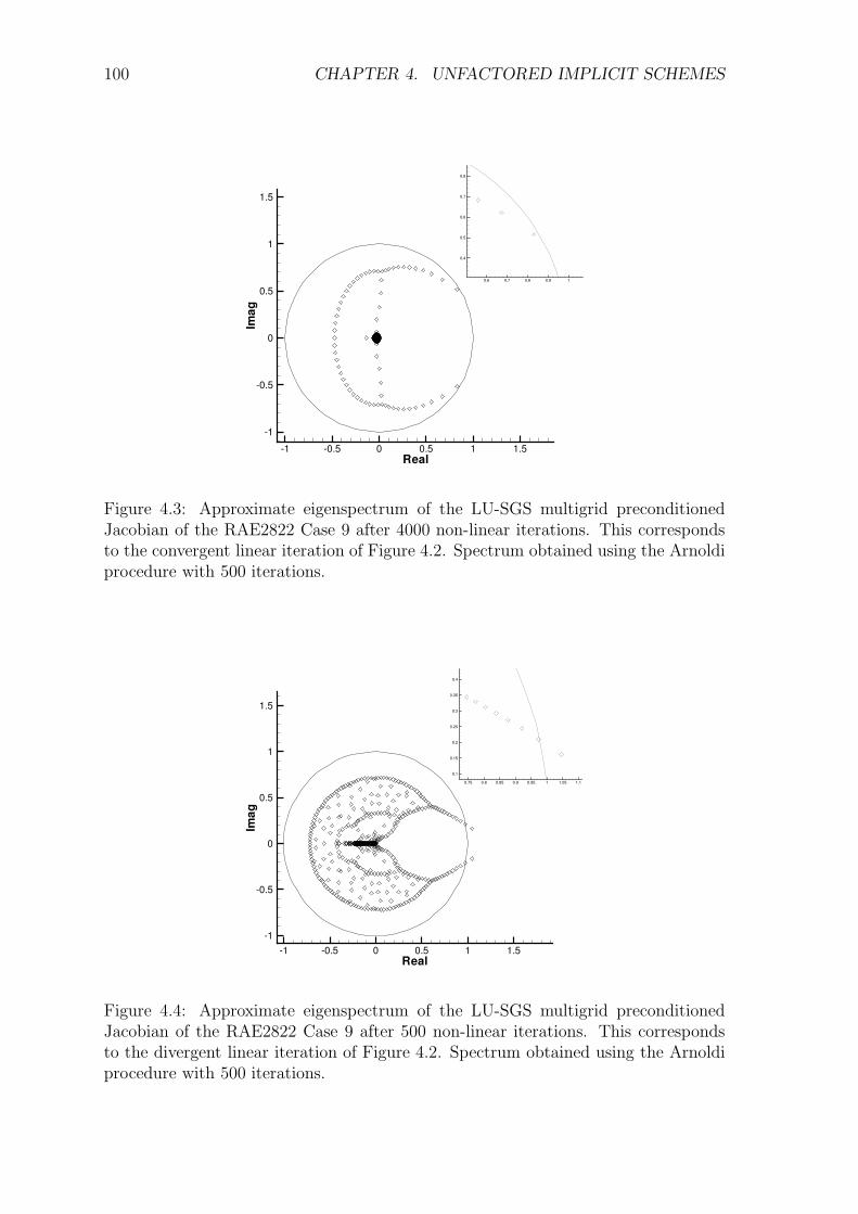
100 CHAPTER 4. UNFACTORED IMPLICIT SCHEMES
Real
Imag
-1 -0.5 0 0.5 1 1.5
-1
-0.5
0
0.5
1
1.5
0.6 0.7 0.8 0.9 1
0.4
0.5
0.6
0.7
0.8
Figure 4.3: Approximate eigenspectrum of the LU-SGS multigrid preconditionedJacobian of the RAE2822 Case 9 after 4000 non-linear iterations. This correspondsto the convergent linear iteration of Figure 4.2. Spectrum obtained using the Arnoldiprocedure with 500 iterations.
Real
Imag
-1 -0.5 0 0.5 1 1.5-1
-0.5
0
0.5
1
1.5
0.75 0.8 0.85 0.9 0.95 1 1.05 1.1
0.1
0.15
0.2
0.25
0.3
0.35
0.4
Figure 4.4: Approximate eigenspectrum of the LU-SGS multigrid preconditionedJacobian of the RAE2822 Case 9 after 500 non-linear iterations. This correspondsto the divergent linear iteration of Figure 4.2. Spectrum obtained using the Arnoldiprocedure with 500 iterations.
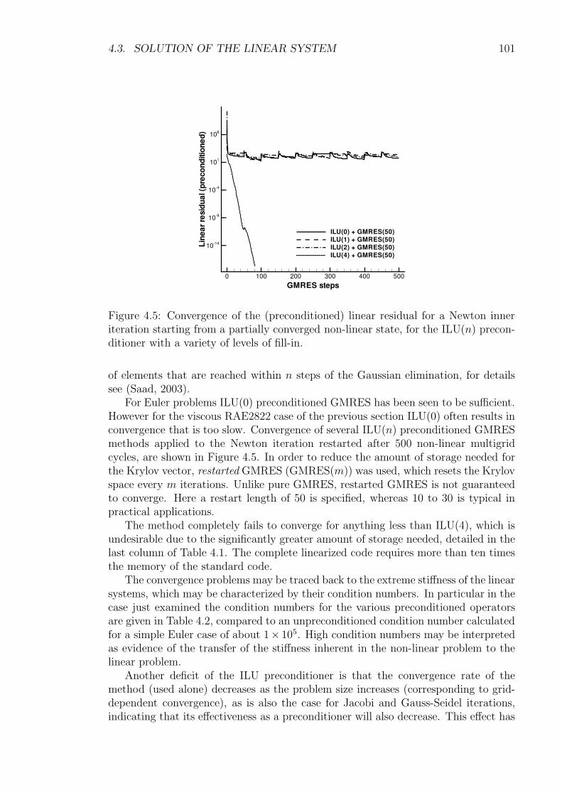
4.3. SOLUTION OF THE LINEAR SYSTEM 101
GMRES steps
Line
arre
sidu
al(p
reco
nditi
oned
)
0 100 200 300 400 500
10-14
10-9
10-4
101
106
ILU(0) + GMRES(50)ILU(1) + GMRES(50)ILU(2) + GMRES(50)ILU(4) + GMRES(50)
Figure 4.5: Convergence of the (preconditioned) linear residual for a Newton inneriteration starting from a partially converged non-linear state, for the ILU(n) precon-ditioner with a variety of levels of fill-in.
of elements that are reached within n steps of the Gaussian elimination, for detailssee (Saad, 2003).
For Euler problems ILU(0) preconditioned GMRES has been seen to be sufficient.However for the viscous RAE2822 case of the previous section ILU(0) often results inconvergence that is too slow. Convergence of several ILU(n) preconditioned GMRESmethods applied to the Newton iteration restarted after 500 non-linear multigridcycles, are shown in Figure 4.5. In order to reduce the amount of storage needed forthe Krylov vector, restarted GMRES (GMRES(m)) was used, which resets the Krylovspace every m iterations. Unlike pure GMRES, restarted GMRES is not guaranteedto converge. Here a restart length of 50 is specified, whereas 10 to 30 is typical inpractical applications.
The method completely fails to converge for anything less than ILU(4), which isundesirable due to the significantly greater amount of storage needed, detailed in thelast column of Table 4.1. The complete linearized code requires more than ten timesthe memory of the standard code.
The convergence problems may be traced back to the extreme stiffness of the linearsystems, which may be characterized by their condition numbers. In particular in thecase just examined the condition numbers for the various preconditioned operatorsare given in Table 4.2, compared to an unpreconditioned condition number calculatedfor a simple Euler case of about 1× 10⁵. High condition numbers may be interpretedas evidence of the transfer of the stiffness inherent in the non-linear problem to thelinear problem.
Another deficit of the ILU preconditioner is that the convergence rate of themethod (used alone) decreases as the problem size increases (corresponding to grid-dependent convergence), as is also the case for Jacobi and Gauss-Seidel iterations,indicating that its effectiveness as a preconditioner will also decrease. This effect has
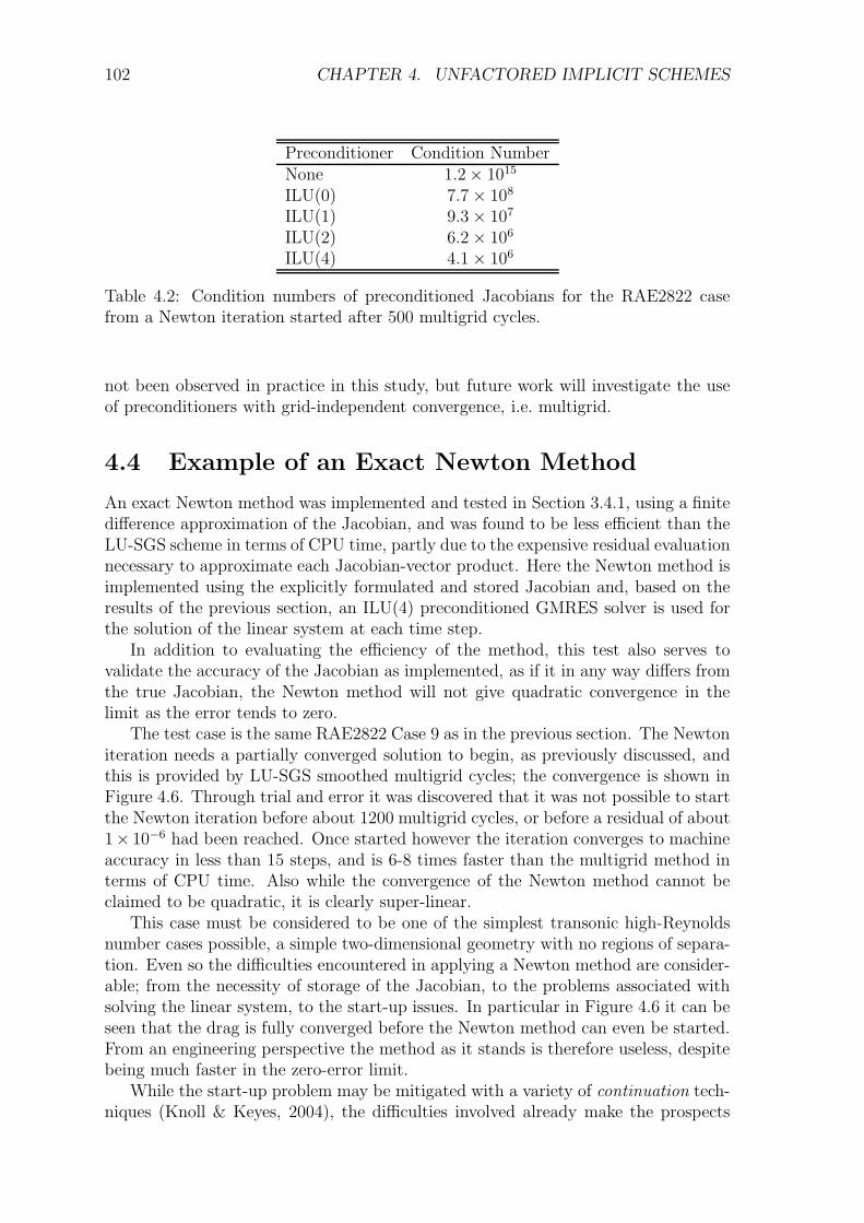
102 CHAPTER 4. UNFACTORED IMPLICIT SCHEMES
Preconditioner Condition NumberNone 1.2× 10¹⁵
ILU(0) 7.7× 10⁸
ILU(1) 9.3× 10⁷
ILU(2) 6.2× 10⁶
ILU(4) 4.1× 10⁶
Table 4.2: Condition numbers of preconditioned Jacobians for the RAE2822 casefrom a Newton iteration started after 500 multigrid cycles.
not been observed in practice in this study, but future work will investigate the useof preconditioners with grid-independent convergence, i.e. multigrid.
4.4 Example of an Exact Newton Method
An exact Newton method was implemented and tested in Section 3.4.1, using a finitedifference approximation of the Jacobian, and was found to be less efficient than theLU-SGS scheme in terms of CPU time, partly due to the expensive residual evaluationnecessary to approximate each Jacobian-vector product. Here the Newton method isimplemented using the explicitly formulated and stored Jacobian and, based on theresults of the previous section, an ILU(4) preconditioned GMRES solver is used forthe solution of the linear system at each time step.
In addition to evaluating the efficiency of the method, this test also serves tovalidate the accuracy of the Jacobian as implemented, as if it in any way differs fromthe true Jacobian, the Newton method will not give quadratic convergence in thelimit as the error tends to zero.
The test case is the same RAE2822 Case 9 as in the previous section. The Newtoniteration needs a partially converged solution to begin, as previously discussed, andthis is provided by LU-SGS smoothed multigrid cycles; the convergence is shown inFigure 4.6. Through trial and error it was discovered that it was not possible to startthe Newton iteration before about 1200 multigrid cycles, or before a residual of about1× 10−6 had been reached. Once started however the iteration converges to machineaccuracy in less than 15 steps, and is 6-8 times faster than the multigrid method interms of CPU time. Also while the convergence of the Newton method cannot beclaimed to be quadratic, it is clearly super-linear.
This case must be considered to be one of the simplest transonic high-Reynoldsnumber cases possible, a simple two-dimensional geometry with no regions of separa-tion. Even so the difficulties encountered in applying a Newton method are consider-able; from the necessity of storage of the Jacobian, to the problems associated withsolving the linear system, to the start-up issues. In particular in Figure 4.6 it can beseen that the drag is fully converged before the Newton method can even be started.From an engineering perspective the method as it stands is therefore useless, despitebeing much faster in the zero-error limit.
While the start-up problem may be mitigated with a variety of continuation tech-niques (Knoll & Keyes, 2004), the difficulties involved already make the prospects
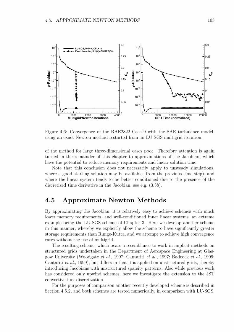
4.5. APPROXIMATE NEWTON METHODS 103
Multigrid/Newton Iterations
ρ-R
esid
ual
CD
0 1000 2000 3000 4000
10-14
10-12
10-10
10-8
10-6
10-4
10-2
100
0
0.05
0.1
0.15
0.2
0.25
0.3LU-SGS, MG4w, CFL=10Exact Jacobian, ILU(4)+GMRES(30)
CPU Time (normalized)
ρ-R
esid
ual
CD
0 5000 10000 15000 20000
10-14
10-12
10-10
10-8
10-6
10-4
10-2
100
0
0.05
0.1
0.15
0.2
0.25
0.3
Figure 4.6: Convergence of the RAE2822 Case 9 with the SAE turbulence model,using an exact Newton method restarted from an LU-SGS multigrid iteration.
of the method for large three-dimensional cases poor. Therefore attention is againturned in the remainder of this chapter to approximations of the Jacobian, whichhave the potential to reduce memory requirements and linear solution time.
Note that this conclusion does not necessarily apply to unsteady simulations,where a good starting solution may be available (from the previous time step), andwhere the linear system tends to be better conditioned due to the presence of thediscretized time derivative in the Jacobian, see e.g. (3.38).
4.5 Approximate Newton Methods
By approximating the Jacobian, it is relatively easy to achieve schemes with muchlower memory requirements, and well-conditioned inner linear systems; an extremeexample being the LU-SGS scheme of Chapter 3. Here we develop another schemein this manner, whereby we explicitly allow the scheme to have significantly greaterstorage requirements than Runge-Kutta, and we attempt to achieve high convergencerates without the use of multigrid.
The resulting scheme, which bears a resemblance to work in implicit methods onstructured grids undertaken in the Department of Aerospace Engineering at Glas-gow University (Woodgate et al., 1997; Cantariti et al., 1997; Badcock et al., 1999;Cantariti et al., 1999), but differs in that it is applied on unstructured grids, therebyintroducing Jacobians with unstructured sparsity patterns. Also while previous workhas considered only upwind schemes, here we investigate the extension to the JSTconvective flux discretization.
For the purposes of comparison another recently developed scheme is described inSection 4.5.2, and both schemes are tested numerically, in comparison with LU-SGS.
104 CHAPTER 4. UNFACTORED IMPLICIT SCHEMES
4.5.1 1st-Order Jacobian Krylov Implicit Method (FOKI)
The method developed here will be referred to as the First-Order Jacobian, Krylov Im-plicit (FOKI) method, as it uses an explicitly calculated and stored Jacobian based onfirst-order convective fluxes, the resulting system being solved using a preconditionedKrylov method (in the following GMRES). The turbulence equations are decoupledfrom the mean flow equations, and solved using a separate Krylov iteration. It isalways used without multigrid.
Approximation of the Jacobian
The chief aim of this approximation is to reduce the stencil of the discretization toimmediate neighbours of a node only, leading to a corresponding reduction in thesparse fill-in of the Jacobian. Such a simplification results in a reduction of thememory requirements of the solver with Jacobian storage to less than three-timesthose of the non-linear solver, and the system can be solved in a time equivalentto less than 1% of that required for the non-linear system. Further the immediateneighbour fill-in allows the storage of the off-diagonal entries of the Jacobian on theedges of the unstructured grid (as opposed to being stored in a special sparse matrixdata structure), making a Jacobian-vector multiplication a familiar loop over all gridedges.
This stencil reduction may be achieved by constructing the Jacobian from deriva-tives of first-order convective fluxes, and TSL viscous and turbulence diffusion fluxes(see Section 2.8.1). The stencil of the turbulence discretization consists only of im-mediate neighbours anyway, and therefore is treated without approximation.
The most sensitive issue is the simplification of the convective fluxes. For anupwind discretization the first-order generalization is natural; the use of constantface-reconstruction rather than affine reconstruction reduces the stencil in the re-quired manner. In order to improve the Jacobian approximation somewhat, once theexpression for the flux derivative has been obtained from the first-order upwind flux,values reconstructed onto the cell faces are used instead of cell-centered values in theexpression.
For the JST scheme used here the situation is not as clear. For convenience theJST flux is repeated here, from (2.28):
f JSTij (W ;nij) =
1
2
(f c(Wi) + f c(Wj)
)· nij
− 1
2
∣∣λcij∣∣ε
(2)ij (Wj −Wi)− ε(4)
ij (Lj(W )− Li(W ))
, (4.6)
where in additionLi(W ) =
∑
k∈N(i)
(Wk −Wi), (4.7)
in the interior of the field.
4.5. APPROXIMATE NEWTON METHODS 105
xi−2 xi−1 xi xi+1 xi+2
2nd difference +1 −2 +14th difference +1 −4 +6 −4 +14th chopped −4 +6 −4
Table 4.3: Second and fourth difference operators in one-dimension. Also a fourthdifference that has been “chopped” in order to reduce its stencil.
There are two principal possibilities to reduce the stencil: (a) use purely second-order dissipation, neglecting the term involving L(W ) in (4.6), so that
f cij(Wi,Wj;nij) =1
2
(f c(Wi) + f c(Wj)
)· nij
− 1
2
∣∣λcij∣∣χ(ε
(2)ij , ε
(4)ij )(Wj −Wi)
, (4.8)
is the flux to be differentiated, as in LU-SGS, or (b) explicitly neglect derivatives ofthe dissipation with respect to next-neighbours, whereby derivatives with respect tofourth-order dissipation terms are included for the immediate neighbours.
Given that the solution is smooth almost everywhere, the true residual will containa 4th difference operator almost everywhere, and neither of these simplifications issatisfactory. Consider Table 4.3, which gives the weights of 2nd differences, 4th differ-ences, and the “chopped” 4th differences of option (b) in 1D. The operator of option(a) is completely at variance with the 4th difference operator, with even the signs ofthe corresponding weights differing. On the other hand choosing option (b) (the lastrow of Table 4.3) results in a system that is considerably more difficult to solve thanthe full unapproximated system, even though it is more diagonally dominant. Thiscould be understood to be a result of fact that the chopped fourth-order dissipationoperator contains a large second-order anti-dissipation component. In the absenceof a really satisfactory approximation, the pure second-order dissipation operator isused in the following.
It remains to choose the function χ, which is necessary as both ε(2) and ε(4) arezero in particular regions of the solution, but are never zero together due to the shockswitch. Simply using χ = k(2), the constant coefficient of second-order dissipation,is equivilent to the Jacobian of a Lax-Friedrichs scheme as for LU-SGS. Better non-linear convergence can be obtained with the choice of (Wong & Zingg, 2005), namely
χ(ε(2), ε(4)) = ε(2) + σε(4). (4.9)
Numerical experiments suggest that a value of σ in the range 10− 20 is appropriate.In the remainder of this thesis σ = 15 is used.
Decoupled Turbulence Treatment
As in the case of LU-SGS, the turbulence equations are decoupled from the mean-flow equations in the FOKI method. However, in order to increase the flexibilityof the turbulence treatment the turbulence equations are also formulated and solved
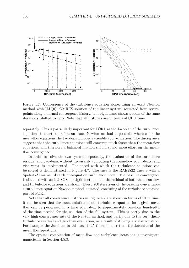
106 CHAPTER 4. UNFACTORED IMPLICIT SCHEMES
CPU time (normalized)ρ-
Res
idua
l,ν-
Res
idua
l0 20 40 60 80
10-14
10-12
10-10
10-8
10-6
10-4
CPU time (normalized)
ρ-R
esid
ual,
ν-R
esid
ual
0 5000 10000 15000
10-14
10-12
10-10
10-8
10-6
10-4
10-2
100 Lusgs, MG4w -ρ-ResidualLusgs, MG4w -ν-ResidualNewton on Turb. Eqns, Restarted
Figure 4.7: Convergence of the turbulence equation alone, using an exact Newtonmethod with ILU(0)+GMRES solution of the linear system, restarted from severalpoints along a normal convergence history. The right-hand shows a zoom of the sameiterations, shifted to zero. Note that all histories are in terms of CPU time.
separately. This is particularly important for FOKI, as the Jacobian of the turbulenceequations is exact, therefore an exact Newton method is possible, whereas for themean-flow equations the Jacobian includes a sizeable approximation. The discrepancysuggests that the turbulence equations will converge much faster than the mean-flowequations, and therefore a balanced method should spend more effort on the mean-flow convergence.
In order to solve the two systems separately, the evaluation of the turbulenceresidual and Jacobian, without necessarily computing the mean-flow equivalents, andvice versa, is implemented. The speed with which the turbulence equations canbe solved is demonstrated in Figure 4.7. The case is the RAE2822 Case 9 with aSpalart-Allmaras Edwards one-equation turbulence model. The baseline convergenceis obtained with an LU-SGS multigrid method, and the residual of both the mean-flowand turbulence equations are shown. Every 200 iterations of the baseline convergencea turbulence equation Newton method is started, consisting of the turbulence equationpart of FOKI.
Note that all convergence histories in Figure 4.7 are shown in terms of CPU time;it can be seen that the exact solution of the turbulence equation for a given meanflow can be performed in a time equivalent to approximately one-four hundredthof the time needed for the solution of the full system. This is partly due to thevery high convergence rate of the Newton method, and partly due to the very cheapturbulence residual and Jacobian evaluation, as a result of it being a scalar equation.For example the Jacobian in this case is 25 times smaller than the Jacobian of themean flow equations.
The optimal combination of mean-flow and turbulence iterations is investigatednumerically in Section 4.5.3.
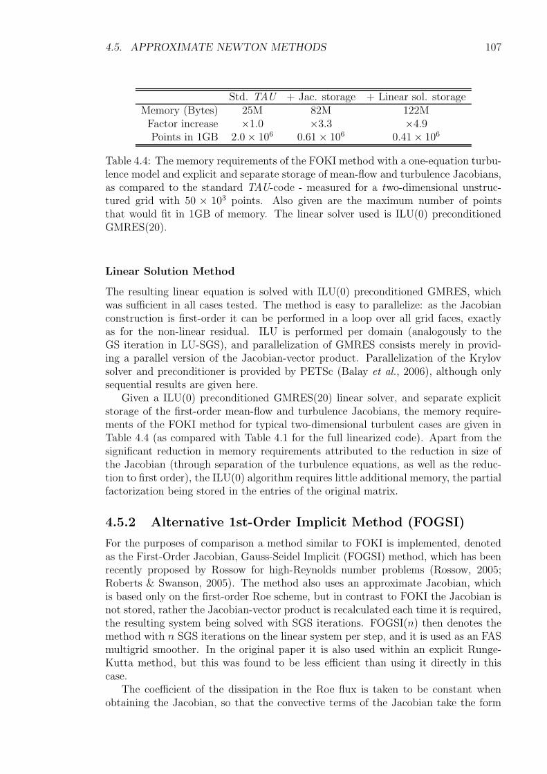
4.5. APPROXIMATE NEWTON METHODS 107
Std. TAU + Jac. storage + Linear sol. storageMemory (Bytes) 25M 82M 122M
Factor increase ×1.0 ×3.3 ×4.9Points in 1GB 2.0× 10⁶ 0.61× 10⁶ 0.41× 10⁶
Table 4.4: The memory requirements of the FOKI method with a one-equation turbu-lence model and explicit and separate storage of mean-flow and turbulence Jacobians,as compared to the standard TAU-code - measured for a two-dimensional unstruc-tured grid with 50 × 103 points. Also given are the maximum number of pointsthat would fit in 1GB of memory. The linear solver used is ILU(0) preconditionedGMRES(20).
Linear Solution Method
The resulting linear equation is solved with ILU(0) preconditioned GMRES, whichwas sufficient in all cases tested. The method is easy to parallelize: as the Jacobianconstruction is first-order it can be performed in a loop over all grid faces, exactlyas for the non-linear residual. ILU is performed per domain (analogously to theGS iteration in LU-SGS), and parallelization of GMRES consists merely in provid-ing a parallel version of the Jacobian-vector product. Parallelization of the Krylovsolver and preconditioner is provided by PETSc (Balay et al., 2006), although onlysequential results are given here.
Given a ILU(0) preconditioned GMRES(20) linear solver, and separate explicitstorage of the first-order mean-flow and turbulence Jacobians, the memory require-ments of the FOKI method for typical two-dimensional turbulent cases are given inTable 4.4 (as compared with Table 4.1 for the full linearized code). Apart from thesignificant reduction in memory requirements attributed to the reduction in size ofthe Jacobian (through separation of the turbulence equations, as well as the reduc-tion to first order), the ILU(0) algorithm requires little additional memory, the partialfactorization being stored in the entries of the original matrix.
4.5.2 Alternative 1st-Order Implicit Method (FOGSI)
For the purposes of comparison a method similar to FOKI is implemented, denotedas the First-Order Jacobian, Gauss-Seidel Implicit (FOGSI) method, which has beenrecently proposed by Rossow for high-Reynolds number problems (Rossow, 2005;Roberts & Swanson, 2005). The method also uses an approximate Jacobian, whichis based only on the first-order Roe scheme, but in contrast to FOKI the Jacobian isnot stored, rather the Jacobian-vector product is recalculated each time it is required,the resulting system being solved with SGS iterations. FOGSI(n) then denotes themethod with n SGS iterations on the linear system per step, and it is used as an FASmultigrid smoother. In the original paper it is also used within an explicit Runge-Kutta method, but this was found to be less efficient than using it directly in thiscase.
The coefficient of the dissipation in the Roe flux is taken to be constant whenobtaining the Jacobian, so that the convective terms of the Jacobian take the form
108 CHAPTER 4. UNFACTORED IMPLICIT SCHEMES
A ± |A| (where A = ∂f c/∂W ), which is evaluated using flow variables on the gridfaces with either constant or affine reconstruction.
The core idea of the method is to make the product (A ± |A|) · ∆W , for someflow state update ∆W , very computationally efficient, thereby making the entiremethod efficient. This is achieved by firstly working entirely in primitive variables,and secondly rewriting the above product in terms of the Mach number as follows (intwo-dimensions):
A± |A| =
V ± ρnxM± ρnyM
± ± 1aM
0 V ± ± n2xaM ±nxnyaM nx
ρM±
0 nxnyaM V ± ± n2yaM
nyρM±
0 nxρa2M± nyρa
2M± V ± ± aM
, (4.10)
where V = U · n, V ± = V ± |V |, M± = (1±M0), M = 1− |M0|, and
M0 =
1 M > 1
M −1 ≤M ≤ 1
−1 M < −1
.
This is not an approximation to the expression A± |A|, purely a rewrite, in a similarvein to the efficient calculation of |A| due to Turkel in conservative variables (Turkel,1988). The values V ±, M± and M are calculated once at the beginning of a non-linear step and stored on the faces of the grid, further reducing the computationalcost.
In the implementation described here the viscous Jacobians are based on TSLfluxes assuming constant viscosity, and the convective Jacobians are based on flowvalues reconstructed on the grid faces. Also a one-equation turbulence model is used,and differentiated exactly, in contrast to (Rossow, 2005) where an algebraic model isused. Another difference to previous results involves the boundary conditions, whichare also treated exactly in the Jacobian in this case. The inverse of the block diagonalof the Jacobian is calculated explicitly using Gaussian elimination once, and storeduntil the Jacobian is recalculated. This was found by the present author to be fasterthan the method proposed by the originator, of performing a few GS iterations onthe block diagonal at each linear iteration. It has the disadvantage of increasing thememory requirements of the scheme.
In summary the distinguishing differences from FOKI are the absence of anystorage of the Jacobian, the avoidance of Krylov methods in favour of simpler GSiterations, the use as an FAS multigrid smoother, and the lack of explicit separationof mean-flow and turbulence equations (although this latter is of course possiblein FOGSI too). Being based on a Roe flux, FOGSI performs well with upwind andcentral with matrix-dissipation schemes on the RHS, but poorly (in fact it is unstablein most cases) with the scalar dissipation scheme as currently used in TAU.
4.5.3 Numerical Comparison of LU-SGS, FOKI and FOGSI
In order to initially separate convergence behaviour due to the turbulence equationsfrom that involving only the mean flow equations, we consider a laminar test case,
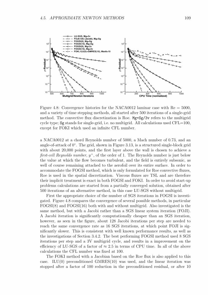
4.5. APPROXIMATE NEWTON METHODS 109
CPU Time (normalized)
ρ-R
esid
ual
0 200 400 600 800 100010-12
10-10
10-8
10-6
10-4
10-2
100
Multigrid/Newton Iteratons
ρ-R
esid
ual
500 600 700 800 900 100010-12
10-10
10-8
10-6
10-4
10-2
100
LU-SGS, Mg=3vFOJI(128) (Jacobi), Mg=SgFOGSI(8), Mg=SgFOGSI(16), Mg=SgFOGSI(8), Mg=3vFOGSI(16), Mg=3vFOKI, ILU(0)+GMRES(10), MaxIt=10
Figure 4.8: Convergence histories for the NACA0012 laminar case with Re = 5000,and a variety of time stepping methods, all started after 500 iterations of a single-gridmethod. The convective flux discretization is Roe. Mg=Sg/3v refers to the multigridcycle type; Sg stands for single-grid, i.e. no multigrid. All calculations used CFL=100,except for FOKI which used an infinite CFL number.
a NACA0012 at a chord Reynolds number of 5000, a Mach number of 0.73, and anangle-of-attack of 0. The grid, shown in Figure 3.13, is a structured single-block gridwith about 20,000 points, and the first layer above the wall is chosen to achieve afirst-cell Reynolds number, y+, of the order of 1. The Reynolds number is just belowthe value at which the flow becomes turbulent, and the field is entirely subsonic, aswell of course remaining attached to the aerofoil over its entire surface. In order toaccommodate the FOGSI method, which is only formulated for Roe convective fluxes,Roe is used in the spatial discretization. Viscous fluxes are TSL and are thereforetheir implicit treatment is exact in both FOGSI and FOKI. In order to avoid start-upproblems calculations are started from a partially converged solution, obtained after500 iterations of an alternative method, in this case LU-SGS without multigrid.
First the appropriate choice of the number of SGS iterations in FOGSI is investi-gated. Figure 4.8 compares the convergence of several possible methods, in particularFOGSI(8) and FOGSI(16) both with and without multigrid. Also investigated is thesame method, but with a Jacobi rather than a SGS linear system iteration (FOJI).A Jacobi iteration is significantly computationally cheaper than an SGS iteration,however, as seen in the figure, about 128 Jacobi iterations per step are needed toreach the same convergence rate as 16 SGS iterations, at which point FOJI is sig-nificantly slower. This is consistent with well known performance results, as well asthe investigations of Section 3.4.2. The best performing FOGSI method used 8 SGSiterations per step and a 3V multigrid cycle, and results in a improvement on theefficiency of LU-SGS of a factor of ≈ 2.5 in terms of CPU time. In all of the abovecalculations the CFL number was fixed at 100.
The FOKI method with a Jacobian based on the Roe flux is also applied to thiscase. ILU(0) preconditioned GMRES(10) was used, and the linear iteration wasstopped after a factor of 100 reduction in the preconditioned residual, or after 10
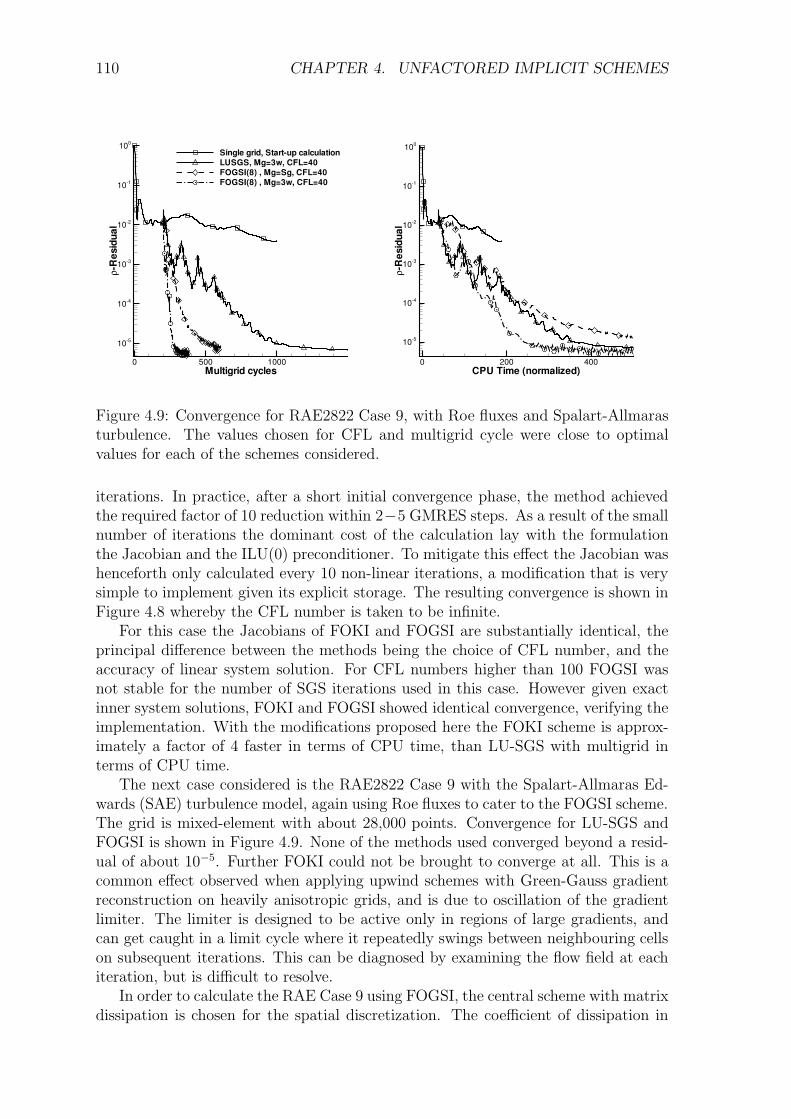
110 CHAPTER 4. UNFACTORED IMPLICIT SCHEMES
CPU Time (normalized)
ρ-R
esid
ual
0 200 400
10-5
10-4
10-3
10-2
10-1
100
Multigrid cycles
ρ-R
esid
ual
0 500 1000
10-5
10-4
10-3
10-2
10-1
100
Single grid, Start-up calculationLUSGS, Mg=3w, CFL=40FOGSI(8) , Mg=Sg, CFL=40FOGSI(8) , Mg=3w, CFL=40
Figure 4.9: Convergence for RAE2822 Case 9, with Roe fluxes and Spalart-Allmarasturbulence. The values chosen for CFL and multigrid cycle were close to optimalvalues for each of the schemes considered.
iterations. In practice, after a short initial convergence phase, the method achievedthe required factor of 10 reduction within 2−5 GMRES steps. As a result of the smallnumber of iterations the dominant cost of the calculation lay with the formulationthe Jacobian and the ILU(0) preconditioner. To mitigate this effect the Jacobian washenceforth only calculated every 10 non-linear iterations, a modification that is verysimple to implement given its explicit storage. The resulting convergence is shown inFigure 4.8 whereby the CFL number is taken to be infinite.
For this case the Jacobians of FOKI and FOGSI are substantially identical, theprincipal difference between the methods being the choice of CFL number, and theaccuracy of linear system solution. For CFL numbers higher than 100 FOGSI wasnot stable for the number of SGS iterations used in this case. However given exactinner system solutions, FOKI and FOGSI showed identical convergence, verifying theimplementation. With the modifications proposed here the FOKI scheme is approx-imately a factor of 4 faster in terms of CPU time, than LU-SGS with multigrid interms of CPU time.
The next case considered is the RAE2822 Case 9 with the Spalart-Allmaras Ed-wards (SAE) turbulence model, again using Roe fluxes to cater to the FOGSI scheme.The grid is mixed-element with about 28,000 points. Convergence for LU-SGS andFOGSI is shown in Figure 4.9. None of the methods used converged beyond a resid-ual of about 10−5. Further FOKI could not be brought to converge at all. This is acommon effect observed when applying upwind schemes with Green-Gauss gradientreconstruction on heavily anisotropic grids, and is due to oscillation of the gradientlimiter. The limiter is designed to be active only in regions of large gradients, andcan get caught in a limit cycle where it repeatedly swings between neighbouring cellson subsequent iterations. This can be diagnosed by examining the flow field at eachiteration, but is difficult to resolve.
In order to calculate the RAE Case 9 using FOGSI, the central scheme with matrixdissipation is chosen for the spatial discretization. The coefficient of dissipation in
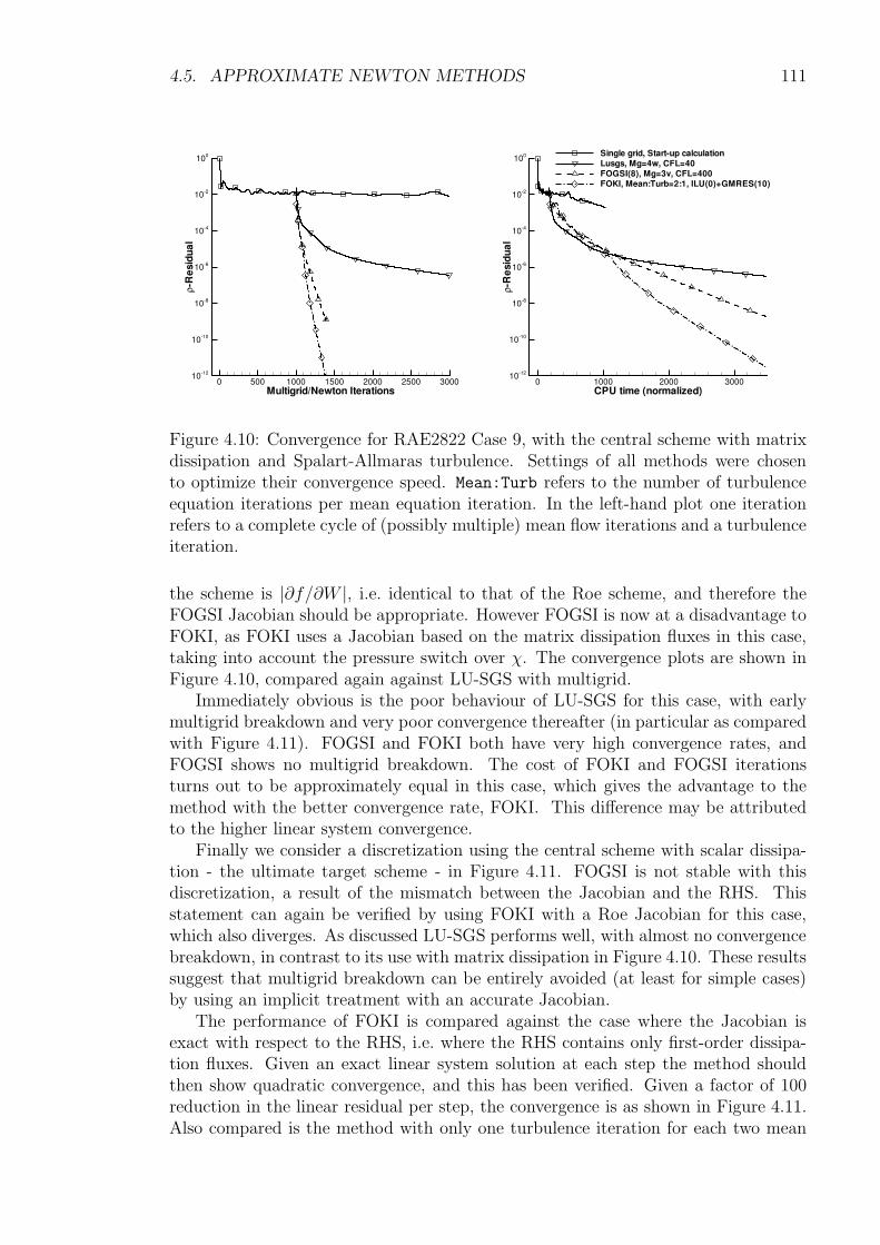
4.5. APPROXIMATE NEWTON METHODS 111
Multigrid/Newton Iterations
ρ-R
esid
ual
0 500 1000 1500 2000 2500 300010-12
10-10
10-8
10-6
10-4
10-2
100
CPU time (normalized)
ρ-R
esid
ual
0 1000 2000 300010-12
10-10
10-8
10-6
10-4
10-2
100 Single grid, Start-up calculationLusgs, Mg=4w, CFL=40FOGSI(8), Mg=3v, CFL=400FOKI, Mean:Turb=2:1, ILU(0)+GMRES(10)
Figure 4.10: Convergence for RAE2822 Case 9, with the central scheme with matrixdissipation and Spalart-Allmaras turbulence. Settings of all methods were chosento optimize their convergence speed. Mean:Turb refers to the number of turbulenceequation iterations per mean equation iteration. In the left-hand plot one iterationrefers to a complete cycle of (possibly multiple) mean flow iterations and a turbulenceiteration.
the scheme is |∂f/∂W |, i.e. identical to that of the Roe scheme, and therefore theFOGSI Jacobian should be appropriate. However FOGSI is now at a disadvantage toFOKI, as FOKI uses a Jacobian based on the matrix dissipation fluxes in this case,taking into account the pressure switch over χ. The convergence plots are shown inFigure 4.10, compared again against LU-SGS with multigrid.
Immediately obvious is the poor behaviour of LU-SGS for this case, with earlymultigrid breakdown and very poor convergence thereafter (in particular as comparedwith Figure 4.11). FOGSI and FOKI both have very high convergence rates, andFOGSI shows no multigrid breakdown. The cost of FOKI and FOGSI iterationsturns out to be approximately equal in this case, which gives the advantage to themethod with the better convergence rate, FOKI. This difference may be attributedto the higher linear system convergence.
Finally we consider a discretization using the central scheme with scalar dissipa-tion - the ultimate target scheme - in Figure 4.11. FOGSI is not stable with thisdiscretization, a result of the mismatch between the Jacobian and the RHS. Thisstatement can again be verified by using FOKI with a Roe Jacobian for this case,which also diverges. As discussed LU-SGS performs well, with almost no convergencebreakdown, in contrast to its use with matrix dissipation in Figure 4.10. These resultssuggest that multigrid breakdown can be entirely avoided (at least for simple cases)by using an implicit treatment with an accurate Jacobian.
The performance of FOKI is compared against the case where the Jacobian isexact with respect to the RHS, i.e. where the RHS contains only first-order dissipa-tion fluxes. Given an exact linear system solution at each step the method shouldthen show quadratic convergence, and this has been verified. Given a factor of 100reduction in the linear residual per step, the convergence is as shown in Figure 4.11.Also compared is the method with only one turbulence iteration for each two mean
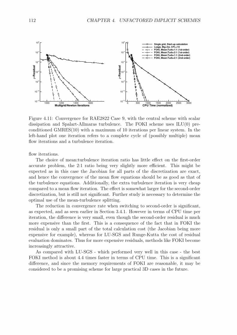
112 CHAPTER 4. UNFACTORED IMPLICIT SCHEMES
CPU Time (normalized)
ρ-R
esid
ual
0 500 1000 1500 2000 2500 300010-12
10-10
10-8
10-6
10-4
10-2
100
Single grid, Start-up calculationLusgs, Mg=3w, CFL=10FOKI, Mean:Turb=1:1 (1st-order)FOKI, Mean:Turb=2:1 (1st-order)FOKI, Mean:Turb=1:1 (2nd-order)FOKI, Mean:Turb=2:1 (2nd-order)
Multigrid/Newton Iterations
ρ-R
esid
ual
1000 1200 1400 160010-12
10-10
10-8
10-6
10-4
10-2
100
Figure 4.11: Convergence for RAE2822 Case 9, with the central scheme with scalardissipation and Spalart-Allmaras turbulence. The FOKI scheme uses ILU(0) pre-conditioned GMRES(10) with a maximum of 10 iterations per linear system. In theleft-hand plot one iteration refers to a complete cycle of (possibly multiple) meanflow iterations and a turbulence iteration.
flow iterations.The choice of mean:turbulence iteration ratio has little effect on the first-order
accurate problem, the 2:1 ratio being very slightly more efficient. This might beexpected as in this case the Jacobian for all parts of the discretization are exact,and hence the convergence of the mean flow equations should be as good as that ofthe turbulence equations. Additionally, the extra turbulence iteration is very cheapcompared to a mean flow iteration. The effect is somewhat larger for the second-orderdiscretization, but is still not significant. Further study is necessary to determine theoptimal use of the mean-turbulence splitting.
The reduction in convergence rate when switching to second-order is significant,as expected, and as seen earlier in Section 3.4.1. However in terms of CPU time periteration, the difference is very small, even though the second-order residual is muchmore expensive than the first. This is a consequence of the fact that in FOKI theresidual is only a small part of the total calculation cost (the Jacobian being moreexpensive for example), whereas for LU-SGS and Runge-Kutta the cost of residualevaluation dominates. Thus for more expensive residuals, methods like FOKI becomeincreasingly attractive.
As compared with LU-SGS - which performed very well in this case - the bestFOKI method is about 4.4 times faster in terms of CPU time. This is a significantdifference, and since the memory requirements of FOKI are reasonable, it may beconsidered to be a promising scheme for large practical 3D cases in the future.
4.6. SUMMARY 113
4.6 Summary
Two methods have been developed about a Jacobian based on first-order convectivefluxes, including boundary conditions, viscous fluxes, and in particular an exact Ja-cobian of the turbulence model. One of the methods uses Gauss-Seidel to solve thelinear system at each non-linear step (FOGSI), and the other uses a preconditionedGMRES algorithm, whereby the linear mean flow and turbulence equations are for-mulated and solved separately, and the method makes no use of multigrid (FOKI).
These schemes were tested on a simple two-dimensional single-element transonicaerofoil configuration, using a hybrid grid consisting of triangles and quadrilaterals,with a high Reynolds number resembling that encountered in practical applications.The FOKI method was seen to consistently out-perform both LU-SGS and FOGSIwith multigrid, and resulted in an improvement in CPU time of a factor of 4-5 overthe LU-SGS scheme, which in turn showed a performance improvement of a factor oftwo over Runge-Kutta.
The code with the FOKI scheme has memory requirements that are about fivetimes those of the standard code, but has the advantage that it is not dependent onmultigrid, and is therefore independent of the unreliable coarse grid agglomerationalgorithm.
It remains to examine the performance, and in particular the robustness of themethod for large three-dimensional test cases, such as those that have been consideredin the context of LU-SGS. The best use of the separation of turbulence and mean-flow must be examined, as well as the start-up procedure. The development of FOKIinto a practically usable scheme represents considerable work, but the method hasbeen shown to be promising.
Chapter 5
The Discrete Adjoint Equations1
5.1 Introduction
We consider gradient-based optimization, characterized by the steepest descent meth-od. A critical component is the evaluation of the gradient of the quantity of interest(the cost function) with respect to the parameterization of the problem (the designvariables). Aerodynamic optimization problems often involve the very detailed pa-rameterization of shapes, and as such a large number of design variables are required.The derivative of a cost function with respect to many design variables can be com-puted in a time only weakly dependent on the number of design variables using theadjoint method. An overview of the situation has been given in Section 1.2.
An ambitious goal of aerodynamic design is the gradient-based optimization ofthree-dimensional high-lift transport aircraft configurations using an unstructuredRANS code. This is an extremely ambitious objective requiring the resolution of anumber of very significant problems before it becomes practicable (Kroll et al., 2004).Some of the difficulties involved are:
(a) The extensive grids necessary in order to accurately resolve the wakes of theindividual elements of the wing (which control the onset of separation on theupper surfaces) and the associated high computational costs (Rudnik et al.,2004). This critical and difficult problem has been tackled in Chapters 3 and 4.
(b) Grid deformation which can robustly handle adjacent bodies with large relativemotion in large grids.
(c) Calculating gradients of the maximum lift CmaxL (Kim et al., 2002), especially
considering that determining the value of CmaxL itself is problematic.
(d) Taking unsteady flow in the non-linear solver and in the design process intoaccount.
(e) The many design variables needed for parameterization of complex 3d shapes(Wild, 2003), which makes an adjoint method for the gradients essential for
1The author is very grateful for the support of Joel Brezillon, who performed all optimiza-tions shown in this chapter in the context of (Dwight & Brezillon, 2006). The author performedthe remainder of the work, in particular the conception and development of the discrete adjointdiscretization and solution method.
114
5.1. INTRODUCTION 115
efficiency. However adjoint techniques have difficulty handling turbulence mod-elling, in the case of the continuous formulation (Nadarajah & Jameson, 2000),or are too memory hungry to be applied to large 3d grids, in the case of thediscrete formulation (Brezillon & Dwight, 2005).
This chapter tackles solely the last problem for the discrete adjoint in the contextof two-dimensional high-lift optimization. There are two principal difficulties asso-ciated with the use of the discrete adjoint: firstly formulating the adjoint requiresdifferentiating the corresponding flow solver per hand, including discrete boundaryconditions, gradient calculations, turbulence models, etc., which as has been seen inChapter 4, is a laborious process, and which must be repeated each time the spatialdiscretization changes. Secondly, depending on the manner of constructing the ad-joint residual, storage of the full discrete flux-Jacobian may be required, which limits3d applications due to memory requirements.
Alternatives to hand-differentiation are being developed, for example complexvariable finite differences (Nielsen & Kleb, 2005; Burdyshaw & Anderson, 2005), andalgorithmic differentiation (Griewank, 2000), but the solution many authors haveused is to perform only an approximate differentiation of a flow solver. For exam-ple by treating the coefficient of artificial viscosity in the Jameson-Schmidt-Turkelscheme (Jameson et al., 1981) as constant it is possible to reduce the constructionof the adjoint residual to two sweeps over the faces of the grid (Mavriplis, 2004;Mavriplis, 2005). Another example is the practice of assuming that the eddy-viscosityis constant, thereby obviating the differentiation of the turbulence model (Kim et al.,2003).
There have, however, been few studies examining the effect these approximationshave on the resulting gradients and optimizations; and this is consequently a matterof pressing interest to the community. It is the purpose of this chapter to determinewhich of these simplifications are acceptable in the context of aerodynamic opti-mization, in the sense of how the convergence of the optimization and its result areaffected. In particular the approximations considered are:
• Adjoint solution based on a 1st-order accurate discretization (FOA),
• Adjoint solution with Thin Shear-Layer viscous fluxes (TSL),
• Assumption of constant coefficients in the JST scheme (CCA),
• Assumption of constant eddy-viscosity (CEV),
• Adjoint solution with alternative turbulence model (ATM).
Each of these approximations is either based on the assumption that the derivativesof the particular terms are negligible, or that they may be replaced with the deriva-tives of similar related terms. Two optimization test cases are examined numericallyfor each approximation: (i) drag reduction of a transonic aerofoil, where the designproblem essentially consists of the removal of the shock, and (ii) drag reduction of ahigh-lift configuration in which a wide variety of flow phenomena are represented, andfor which both compressible and viscous effects, as well as the choice of turbulencemodel are critical. By considering such a wide range of flow phenomena, it is antici-pated that the results obtained will be valid for general two-dimensional aerodynamic
116 CHAPTER 5. THE DISCRETE ADJOINT EQUATIONS
optimizations, and it is hoped that they will also be representative of the situationin three-dimensions.
With this goal the exact discrete adjoint to the unstructured finite volume RANSsolver, the DLR TAU-code, is constructed based on the formulation of the Jacobiandescribed in Chapter 4. The gradients obtained from the exact adjoint are verifiedagainst those obtained using finite differences on the original non-linear routines.Where the approximate adjoint formulations are the result of using a related dis-cretization, as for the adjoint based on 1st-order fluxes, finite differences have againbeen used to verify the implementation. Gradient evaluations and thereafter full op-timizations are then performed with each of the various adjoint approximations, andvariations in gradients, convergence rates and solutions attained are compared.
The solution of the linear adjoint problem is performed using a Krylov subspacemethod with ILU preconditioning, allowing the solution of the adjoint problem in aCPU time equivalent to about 5% of the time required for the main problem. In ad-dition the adjoint fields for multiple cost-functions may be computed simultaneously,further reducing the CPU-time cost of the gradient evaluation.
5.1.1 Overview
Section 5.2 provides a short formal description of the design problem and introducesthe necessary notation. Section 5.3 introduces the adjoint method, and in particularit is shown how it is possible to evaluate the adjoint solution with an effort equivalentto 5% of that needed to evaluate the flow solution itself (Brezillon & Dwight, 2005),making optimization methods that require large numbers of gradient evaluations, suchas the Quasi-Newton Trust Region (QNTR) approach, attractive in an aerodynamicdesign context for the first time.
The simplifying approximations for the Jacobian are described in detail in Sec-tion 5.4. In order to determine whether or not the gradients remain accurate enoughfor use in optimization, and therefore which Jacobian approximations are admissible,each approximation is numerically tested within the conjugate gradient method forthe drag reduction of a transonic single element aerofoil and a multi-element high-liftconfiguration, Section 5.5. It is seen that the Jacobian may be simplified consider-ably without seriously damaging the accuracy of the gradients, and that resultingoptimizations are barely affected (Dwight & Brezillon, 2006).
5.2 Aerodynamic Design Problem
The optimization problem may be stated as follows: minimize I(W,X,D) a cost-function with respect to some set of design variables D, subject to the constraintsR(W,X,D) = 0 and G(X,D) = 0; whereby W and X are functions of D, and R andG are general non-linear operators.
Here I is typically an aerodynamic force integrated over the geometry such aslift, drag or pitching moment, W represents the flow variables, X the computationalmesh, R the residual resulting from the discretization of the fluid flow equations, andG a mesh deformation operator. In particular R is here the finite volume discretiza-tion on an unstructured mesh of the Navier-Stokes equations. Finally D is someparameterization of the geometry and onflow conditions.
5.3. GRADIENTS VIA DISCRETE ADJOINT 117
For problems with a large number of design variables, the most efficient algorithmsare gradient-based, and require the evaluation of dI/dD for each design variable.These gradients may in turn be efficiently evaluated using the adjoint approach.Additional constraints on the problem are also common, such as the specification ofconstant lift and constant pitching moment.
5.2.1 Details of the Discretization
The spatial dicretization is exactly the finite volume discretization of the Navier-Stokes equations described in Chapter 2. The central numerical flux with mixedsecond- and fourth-order scalar dissipation operators is applied (Jameson et al., 1981),see Section 2.6. Viscous and turbulence diffusion fluxes use Green-Gauss gradients av-eraged onto the cell faces, as per (2.75), and thereby have a stencil of next-neighbours.Turbulence convective fluxes are 1st-order upwind, sources use gradients from Green-Gauss.
5.3 Gradients via Discrete Adjoint
The adjoint approach allows the rapid evaluation of dI/dD for a large number ofdesign variables |D|. It can be readily understood by contrasting it with the director primal approach.
5.3.1 Primal Approach
The most direct approach to evaluation of the gradient is to apply the chain rule todI/dD, to give
dI
dD=
∂I
∂W
dW
dD+
∂I
∂X
dX
dD+∂I
∂D,
which is an expression for dI/dD in terms of dW/dD and dX/dD (the remainingquantities being readily calculable). By noting that dR/dD = 0 - as the conditionR = 0 should hold for all D - we have
dR
dD=
∂R
∂W
dW
dD+∂R
∂X
dX
dD+∂R
∂D= 0, (5.1)
a linear system for dW/dD, based on the linearization of the discretized flow equa-tions. Hence to find the sensitivity of I to |D| design variables it is necessary tosolve (5.1) |D| times, and in practice this effort dominates the total cost of the cal-culation.
5.3.2 Adjoint Approach
Instead of applying the chain rule to I, apply it to the Lagrangian:
L(W,X,D,Λ) = I(W,X,D) + ΛTR(W,X,D),
where Λ are known as the adjoint variables. Since R = 0 for all D, L = I for all Λand all D. Hence
dL
dD=
dI
dD, ∀ Λ, D.
118 CHAPTER 5. THE DISCRETE ADJOINT EQUATIONS
Applying the chain rule to L
dL
dD=
∂I
∂W
dW
dD+
∂I
∂X
dX
dD+∂I
∂D
+ ΛT
∂R
∂W
dW
dD+∂R
∂X
dX
dD+∂R
∂D
,
=
∂I
∂W+ ΛT ∂R
∂W
dW
dD+
∂I
∂X+ ΛT ∂R
∂X
dX
dD+
∂I
∂D+ ΛT ∂R
∂D
,(5.2)
after rearranging. The unknown quantity dW/dD may then be eliminated by choos-ing Λ such that (
∂R
∂W
)TΛ = −
(∂I
∂W
)T, (5.3)
whereby the first bracketed term of (5.2) is zero. This is the adjoint equation, andmust be solved only once to evaluate the gradient of a single I with respect to anynumber of design variables. Given Λ, the gradient is
dL
dD=
∂I
∂X+ ΛT ∂R
∂X
dX
dD+
∂I
∂D+ ΛT ∂R
∂D
,
whereby ∂I/∂D and ∂R/∂D are zero for shape-based design variables, and the re-maining unknown term, dX/dD, may be reliably evaluated by finite differences,
∂I
∂X
dX
dD∆Di ≈
I(W,X(D + ε∆Di), D)− I(W,X,D)
ε,
∂R
∂X
dX
dD∆Di ≈
R(W,X(D + ε∆Di), D)−R(W,X,D)
ε,
as the result is relatively insensitive to choice of ε, in contrast to direct approximationof dI/dD by finite differences.
5.3.3 Adjoint of the Grid Deformation
In order to eliminate the use of finite differences for dX/dD, it is possible to use anadjoint approach, thereby removing the expense of deforming the grid in responseto each shape-modifying design variable, which is the dominant cost in the gradientcalculation (Nielsen & Park, 2005). Apply the chain rule to a modified Lagrangian
L(W,X,D,ΛR,ΛG) = I(W,X,D) + ΛTRR(W,X,D) + ΛT
GG(X,D),
where two sets of adjoint variables are used, one for each of the two constraints, togive
dL
dD=
∂I
∂W
dW
dD+
∂I
∂X
dX
dD+∂I
∂D
+ ΛT
R
∂R
∂W
dW
dD+∂R
∂X
dX
dD+∂R
∂D
+ ΛTG
∂G
∂X
dX
dD+∂G
∂D
,
=
∂I
∂W+ ΛT
R
∂R
∂W
dW
dD+
∂I
∂X+ ΛT
R
∂R
∂X+ ΛT
G
∂G
∂X
dX
dD
+
∂I
∂D+ ΛT
R
∂R
∂D+ ΛT
G
∂G
∂D
.
5.3. GRADIENTS VIA DISCRETE ADJOINT 119
Then as before dW/dD may be eliminated by choosing ΛR to satisfy
(∂R
∂W
)TΛR = −
(∂I
∂W
)T, (5.4)
but further dX/dD may be eliminated by choosing ΛG such that
(∂G
∂X
)TΛT = −
(∂I
∂X
)T−(∂R
∂X
)TΛR. (5.5)
Thus only (5.4) and (5.5), must be solved for any number of design variables, afterwhich dI/dD may be written
dI
dD=
∂I
∂D+ ΛT
R
∂R
∂D+ ΛT
G
∂G
∂D. (5.6)
The biggest effort involved is the linearization of the grid deformation operator G,and the evaluation of ∂R/∂X and ∂I/∂X. If however a linear deformation operatoris choosen, its linearization is trivial. This approach is not used in this thesis, but isto be the subject of future work.
5.3.4 Implementation of the Method
Implementation of the above procedure requires the ability to evaluate the quantities(∂R/∂W )TΛ - the adjoint residual - and ∂I/∂W . The Jacobian is the same as theexact Jacobian discussed in Chapter 4, i.e. evaluated by hand and stored explicitly.As it is stored explicitly it is easy to transpose.
The fact that the Jacobian was formulated by differentiating with respect to prim-itive variables poses no problem as long as the cost functions are also differentiatedwith respect to primitive variables. The equations remain in conservative form, andtherefore this choice has no effect on the final solution. Given the explicitly storedJacobian - which must only be constructed once per gradient evaluation, even formultiple cost-functions - assessment of the adjoint residual reduces to a matrix-vectorproduct. Further the availability of the matrix allows the application of ILU precon-ditioned Krylov methods, which have been shown to be very effective if the ILU fill-inlevel is chosen high enough, in Section 4.3. Again this preconditioner must only beconstructed once per calculation.
As the eigenspectrum of the Jacobian and transpose Jacobian are identical, theconvergence rates achieved with Krylov subspace methods for the two resulting linearsystems are guaranteed to be identical, and so the experience gained applying thesemethods in implicit schemes in Chapter 4 may be directly carried over. The result isthat the calculation of the adjoint solution requires only approximately 5% of the timerequired for a non-linear flow calculation - and so forms an insignificant componentof the total time for the optimization. Given that the gradient is much cheaperthan the line search, optimization strategies that rely on many gradient evaluations,such as Quasi-Newton Trust Region (QNTR) (Geiger & Kanzow, 1999), become moreattractive. However, the ILU preconditioner and GMRES method have an associatedmemory cost that further reduces the size of grid that may be calculated in a givenmemory, in this case the requirements for ILU with 4 levels of fill-in and GMRES(30)were given in Chapter 4 in Table 4.1.
120 CHAPTER 5. THE DISCRETE ADJOINT EQUATIONS
Note that a finite difference evaluation of the matrix-vector product, as was donein the Newton method of Section 3.4.1 to avoid calculating the Jacobian explicitly, ismuch more difficult to use for the adjoint residual, as the product with the transposedJacobian is needed. It is necessary to split the field into several sets of grid nodes,such that no two nodes within a set are connected to each other by the stencil of thescheme (Nielsen & Kleb, 2005). Then the product of the Jacobian with the vectorconsisting of ones at the node positions of a given set, and zeros elsewhere, returns avector containing the non-zero entries of the Jacobian in the columns where the nodeswere positioned. This vector is approximated by finite differences. However, becauseof the block structure of the matrix the finite difference must be performed (numberof equations) times for each point set. The method therefore requires 20-30 residualevaluations per adjoint residual, and is thereby more expensive than constructing theJacobian explicitly.
5.4 Approximations of the Discrete Adjoint
In an attempt to reduce the memory requirements of the scheme, the manual effortrequired to adjoint new spatial discretizations, and the computational effort requiredto solve the resulting system, approximations to the adjoint equations are made.The cost is inaccuracies in the resulting gradients. Each approximation is describedhere and its advantages noted, while its accuracy will be numerically assessed inSection 5.5. Throughout no approximation of the boundary conditions is undertaken,as all are treated numerically with a stencil of a single (boundary) point, and thereforeappear only on the diagonal of the Jacobian.
5.4.1 1st-Order Approximation (FOA)
As already noted in reference to simplified Jacobians of the central scheme in thecontext of implicit methods, see Section 4.5.1, by forming the Jacobian of first-orderconvective fluxes rather than second-order, the stencil of the Jacobian is reduced toimmediate neighbours of a point only, and the resulting linear system is much betterconditioned.
Here only simplifications of the JST flux are considered, and the same argumentsas in Section 4.5.1 apply. In particular purely second-order dissipation is used:
f cij(Wi,Wj;nij) =1
2
(f c(Wi) + f c(Wj)
)· nij
− 1
2
∣∣λcij∣∣k(2)(Wj −Wi)
, (5.7)
but rather than specifying the dissipation coefficient as a blend of second- and fourth-order coefficients as in (4.9), a constant dissipation factor k(2) is used, which is in thiscase taken to be equal to k(2) in (2.39), i.e. k(2) = 0.5.
5.4.2 Thin Shear-Layer (TSL) Assumption
The formulation of the viscous fluxes given in Section 5.2.1 has a stencil includingnext-neighbours as a result of the use of gradients based on Green-Gauss. As in the
5.4. APPROXIMATIONS OF THE DISCRETE ADJOINT 121
implicit schemes, this stencil may be reduced to immediate neighbours if the TSLflux is used. However here the approximation has an effect on the converged result ofthe calculation. That the two viscous flux discretizations agree well for complex flowsdoes not necessarily imply that their gradients will agree well. This will be examined.
5.4.3 Constant JST Coefficients Approximation (CCA)
By making the assumption that the ε, θ and |A| in (4.6) are constant, the followingsimplification of the adjoint residual is possible (Mavriplis, 2004). Let L(W ) beas defined in (4.7), and treated in the expression for the convective fluxes as anindependent variable, so that the derivative and adjoint of (4.6) may be writtenrespectively
df c
dW=
∂f c
∂W+∂f c
∂L· ∂L∂W
, (5.8)(
df c
dW
)T
=
(∂f c
∂W
)T
+
(∂L
∂W
)T·(∂f c
∂L
)T
, (5.9)
whereby all matrices on the right-hand sides above have immediate neighbour fill-inonly, ∂f c/∂L is symmetric and ∂L/∂W is trivial.
Memory requirements are then approximately 1.6 times those of the FOA schemeif advantage is taken of the symmetry of ∂f c/∂L, and ∂L/∂W is calculated on-the-fly. Also the matrices may be stored on the edges and nodes of the grid, given whichthe adjoint residual may be evaluated in two loops over all edges by introducing anintermediate variable Λ∗ as follows:
Λ∗ =
(∂f c
∂L
)T
· Λ,(
df c
dW
)T
· Λ =
(∂f c
∂W
)T
· Λ +
(∂L
∂W
)T· Λ∗.
TSL viscous and turbulence diffusion fluxes are used to similarly reduce the memoryrequirements of the viscous flux Jacobian, while the discrete turbulence Jacobians areformed exactly.
The CCA approximation may be justified by noting that the terms in the deriva-tive that are neglected due to the approximation are of higher order in the grid spacingthan the remaining terms. Therefore in the limit of zero cell size the influence of theapproximation tends to zero, see Section 2.6.2.
Compared to FOA, this approach seems very favourable; for only sightly morememory the convective fluxes are sensibly approximated. However the resulting sys-tem is almost as poorly conditioned as the exact system and therefore similarly pow-erful linear solvers are required.
5.4.4 Constant Eddy-Viscosity (CEV) Assumption
One of the most demanding parts of the spatial discretization to differentiate by handis the turbulence model, partly due to the wide variety of blending functions, limiters,
122 CHAPTER 5. THE DISCRETE ADJOINT EQUATIONS
vortex corrections etc., partly because of the many coupling points to the mean-flow equations, and partly because of the enormous selection of models available.More seriously it is very difficult to treat turbulence models in a continuous adjointframework without resorting to continuous-discrete hybrids (Nadarajah & Jameson,2000), hence some simplifying assumption must be made.
By assuming that derivatives of all turbulence quantities with respect to all flowvariables are negligible, all turbulence terms are eliminated. For Spalart-Allmarasthe derivatives of the eddy-viscosity are taken to be zero, for k− ω and k− ε modelsderivatives of k and eddy-viscosity are taken to be zero.
One place where this assumption might be invalid is in the adverse pressure gra-dient region following the shock on a transonic airfoil, where the large eddy-viscosityincreases the surface shear-stress, directly affecting the aerodynamic forces.
5.4.5 Use of an Alternative Turbulence Model (ATM)
The only significant benefit that the CEV assumption confers is the avoidance of handdifferentiating the turbulence model. The similarity in the formulation and results of,for instance, the original Spalart-Allmaras model (SA) (Spalart & Allmaras, 1992),and the modified Spalart-Allmaras-Edwards (SAE) (Edwards & Chandra, 1996), sug-gest that it may be reasonable to use the Jacobian of one as an approximation to theJacobian of the other, and that this may be a better approximation than ignoringturbulence derivatives altogether. If so only one or two models of each type must bedifferentiated in a large code.
SA and SAE differ only in the formulation of the turbulence production term:for SA it is based on a measure of the flow vorticity, see Section 2.11.4, SAE uses ameasure of the shear stress, see Section 2.11.5. Within the boundary-layer the sourceterms are dominated in both models by terms involving the wall-distance, hence themodels are expected to differ most significantly in detached shear-layers and vortices.
Another candidate pair might be Wilcox’s k − ω (Wilcox, 1998), and Mentor’sk − ω SST (Menter, 1993), whereby only SA gradients as an approximation to SAEgradients are numerical evaluated in the following.
5.5 Results and Discussion
We wish to determine which, if any, of the previously described approximate Jaco-bians results in an adjoint gradient evaluation method that is sufficiently accurate foruse in aerodynamic optimization. This is a question that is difficult to answer theoret-ically due to the complexity of the complete optimization process, and the somewhatarbitrary nature of the Jacobian approximations. Instead we investigate concrete op-timization problems numerically and examine how each approximate adjoint solverperforms in each case. In an attempt to obtain results that have a relatively generalvalidity, two significantly different 2d optimization problems are considered repre-senting a variety of industrially relevant flow physics, and - just as importantly - twodifferent optimization algorithms are applied.
The first case is drag reduction of a transonic RAE2822 single element aerofoilat a Reynolds number of 6.5 × 10⁶, and a Mach number of 0.730, whereby the liftmust be held constant at a lift coefficient of 0.8. The computational grid is shown
5.5. RESULTS AND DISCUSSION 123
in Fig. 3.13. The geometry is parameterized using 20 design variables which modifythe camberline of the aerofoil with Hicks-Henne bump functions (Hicks & Henne,1978). The thickness of the aerofoil is not permitted to change, and as a result noadditional geometrical constraints are necessary. The baseline geometry has a strongshock on the upper surface which is the main source of pressure drag; the optimizationproblem therefore substantially consists of the removal of the shock. Two gradient-based algorithms, the Conjugate Gradient (CG) method and the Quasi-Newton TrustRegion (QNTR) method are applied to the problem.
The lift constraint is enforced explicitly by varying the angle of attack duringthe evaluation of the drag in the non-linear RANS solver, the so-called target-liftmode. Because we wish to minimize the drag at the target lift C∗L, rather than atthe preexisting lift CL, the objective function must be modified to consider the liftconstraint consistently (Reuther et al., 1999),
I = CD −(∂CD/∂α)
(∂CL/∂α)(CL − C∗L) , (5.10)
a consequence of which is that the accuracy of the gradients of lift are also importantfor the optimization.
The second optimization test-case is also drag reduction at constant lift, but ofthe three-element high-lift geometry in take-off configuration. The baseline geometryand flow conditions are derived from a test-case defined in the European projectEUROLIFT II (Wild et al., 2005), and operate at a Reynolds number of 14.70× 10⁶
and a Mach number of 0.17146. Constant lift is ensured in the same manner asfor the RAE case. The computational grid is shown in Fig. 3.13 and is structured,whereby the structured topology is not employed by the solvers, all algorithms beingimplemented for general unstructured grids. Only the flap of the configuration isparameterized, and in such a manner that no modification to the composite cleanwing is possible (Brezillon & Wild, 2005). The position and angle of attack of theflap relative to the main element may be changed (the so-called setting parameters),as may the sharpness of the flap’s nose and the shape of the portion of the flap hiddenby the main element (shape parameters). Only the conjugate gradient algorithm isexamined for this case.
5.5.1 Transonic RAE2822 Aerofoil
Firstly exact adjoint gradients are compared with direct finite difference approxi-mations to dI/dD; the gradients of total and viscous drag are plotted in Fig. 5.1.Note that the curves in this figure are “smooth” becuase of the indexing of the designvariables, which parameterize bumps running around the surface of the aerofoil inorder. Both finite differences and the discrete adjoint approximate the gradient ofthe discretized cost-function, and should therefore correspond with each other exactlyon any given grid. It may be seen that the agreement is very good, the discrepanciesapparent in the viscous drag gradients may be attributed to the rounding error infinite differences as a result of the very small absolute values of the gradients. Thisdiscrepancy as a percentage of the total drag gradient is less than 0.5%. The discreteadjoint using the exact Jacobian is thereby taken to be verified for this case.
Next the gradients using the adjoint method with various Jacobian approxima-tions are compared with those of the exact adjoint in Fig. 5.2. TSL and CCA gradients
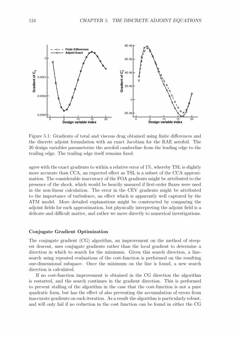
124 CHAPTER 5. THE DISCRETE ADJOINT EQUATIONS
Design variable indexG
radi
ento
fCDv
0 5 10 15 20
-2E-06
0
2E-06
4E-06
6E-06
8E-06
Design variable index
Gra
dien
tofC
D
0 5 10 15 20-0.0003
-0.0002
-0.0001
0
Finite DifferencesAdjoint Exact
Figure 5.1: Gradients of total and viscous drag obtained using finite differences andthe discrete adjoint formulation with an exact Jacobian for the RAE aerofoil. The20 design variables parameterize the aerofoil camberline from the leading edge to thetrailing edge. The trailing edge itself remains fixed.
agree with the exact gradients to within a relative error of 1%, whereby TSL is slightlymore accurate than CCA, an expected effect as TSL is a subset of the CCA approxi-mation. The considerable inaccuracy of the FOA gradients might be attributed to thepresence of the shock, which would be heavily smeared if first-order fluxes were usedin the non-linear calculation. The error in the CEV gradients might be attributedto the importance of turbulence, an effect which is apparently well captured by theATM model. More detailed explanations might be constructed by comparing theadjoint fields for each approximation, but physically interpreting the adjoint field is adelicate and difficult matter, and rather we move directly to numerical investigations.
Conjugate Gradient Optimization
The conjugate gradient (CG) algorithm, an improvement on the method of steep-est descent, uses conjugate gradients rather than the local gradient to determine adirection in which to search for the minimum. Given this search direction, a line-search using repeated evaluations of the cost-function is performed on the resultingone-dimensional subspace. Once the minimum on the line is found, a new searchdirection is calculated.
If no cost-function improvement is obtained in the CG direction the algorithmis restarted, and the search continues in the gradient direction. This is performedto prevent stalling of the algorithm in the case that the cost-function is not a purequadratic form, but has the effect of also preventing the accumulation of errors frominaccurate gradients on each iteration. As a result the algorithm is particularly robust,and will only fail if no reduction in the cost function can be found in either the CG
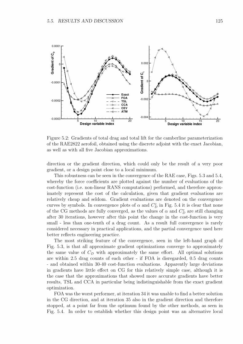
5.5. RESULTS AND DISCUSSION 125
Design variable index
Gra
dien
tofC
L
5 10 15 20-0.004
-0.002
0
0.002
Design variable index
Gra
dien
tofC
D
5 10 15 20-0.0003
-0.0002
-0.0001
0
0.0001
ExactFOATSLCCACEVATM
Figure 5.2: Gradients of total drag and total lift for the camberline parameterizationof the RAE2822 aerofoil, obtained using the discrete adjoint with the exact Jacobian,as well as with all five Jacobian approximations.
direction or the gradient direction, which could only be the result of a very poorgradient, or a design point close to a local minimum.
This robustness can be seen in the convergence of the RAE case, Figs. 5.3 and 5.4,whereby the force coefficients are plotted against the number of evaluations of thecost-function (i.e. non-linear RANS computations) performed, and therefore approx-imately represent the cost of the calculation, given that gradient evaluations arerelatively cheap and seldom. Gradient evaluations are denoted on the convergencecurves by symbols. In convergence plots of α and Cv
D in Fig. 5.4 it is clear that noneof the CG methods are fully converged, as the values of α and Cv
D are still changingafter 30 iterations, however after this point the change in the cost-function is verysmall - less than one-tenth of a drag count. As a result full convergence is rarelyconsidered necessary in practical applications, and the partial convergence used herebetter reflects engineering practice.
The most striking feature of the convergence, seen in the left-hand graph ofFig. 5.3, is that all approximate gradient optimizations converge to approximatelythe same value of CD with approximately the same effort. All optimal solutionsare within 2.5 drag counts of each other - if FOA is disregarded, 0.5 drag counts- and obtained within 30-40 cost-function evaluations. Apparently large deviationsin gradients have little effect on CG for this relatively simple case, although it isthe case that the approximations that showed more accurate gradients have betterresults, TSL and CCA in particular being indistinguishable from the exact gradientoptimization.
FOA was the worst performer, at iteration 34 it was unable to find a better solutionin the CG direction, and at iteration 35 also in the gradient direction and thereforestopped, at a point far from the optimum found by the other methods, as seen inFig. 5.4. In order to establish whether this design point was an alternative local
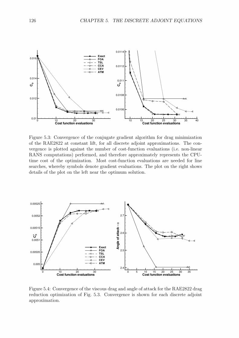
126 CHAPTER 5. THE DISCRETE ADJOINT EQUATIONS
Cost function evaluations
CD
0 10 20 300.01
0.012
0.014
0.016ExactFOATSLCCACEVATM
Cost function evaluationsC
D10 15 20 25 30 35 40
0.0106
0.0108
0.011
0.0112
0.0114
Figure 5.3: Convergence of the conjugate gradient algorithm for drag minimizationof the RAE2822 at constant lift, for all discrete adjoint approximations. The con-vergence is plotted against the number of cost-function evaluations (i.e. non-linearRANS computations) performed, and therefore approximately represents the CPU-time cost of the optimization. Most cost-function evaluations are needed for linesearches, whereby symbols denote gradient evaluations. The plot on the right showsdetails of the plot on the left near the optimum solution.
Cost function evaluations
CDv
0 10 20 30
0.005
0.00505
0.0051
0.00515
0.0052
0.00525
ExactFOATSLCCACEVATM
Cost function evaluations
Ang
leof
atta
ck-α
0 5 10 15 20 25 30 352.4
2.5
2.6
2.7
Figure 5.4: Convergence of the viscous drag and angle of attack for the RAE2822 dragreduction optimization of Fig. 5.3. Convergence is shown for each discrete adjointapproximation.
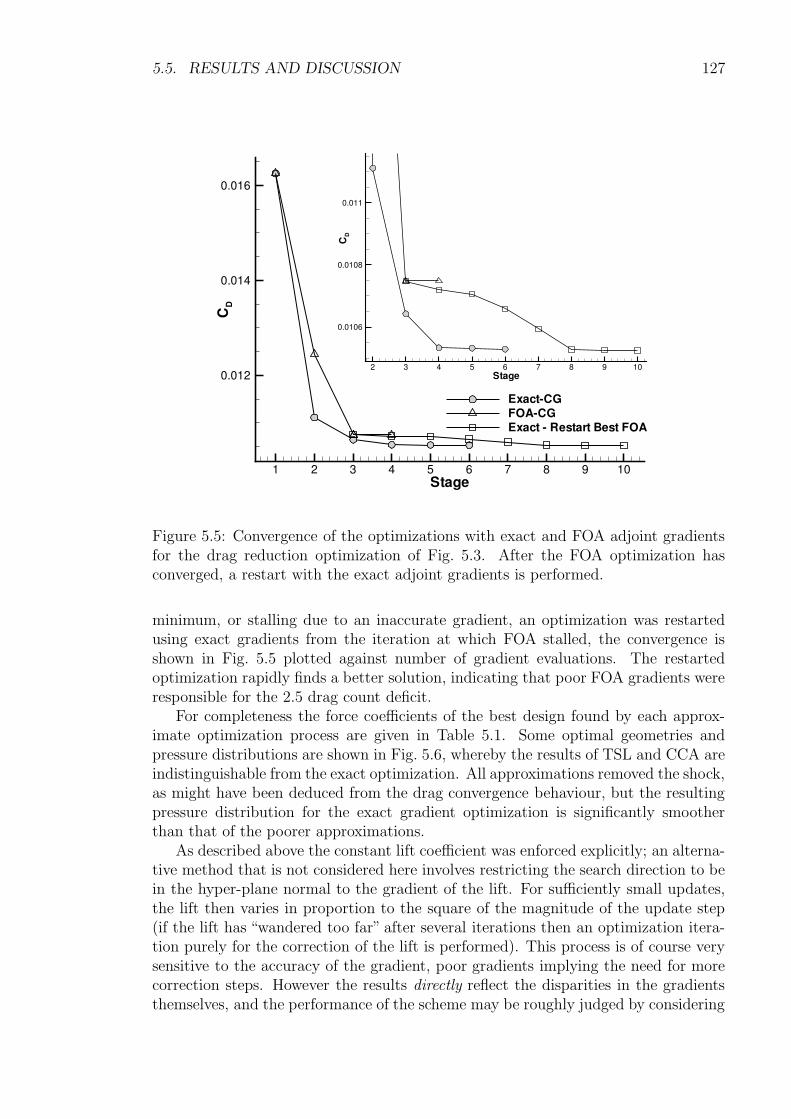
5.5. RESULTS AND DISCUSSION 127
Stage
CD
1 2 3 4 5 6 7 8 9 10
0.012
0.014
0.016
Exact-CGFOA-CGExact -Restart Best FOA
Stage
CD
2 3 4 5 6 7 8 9 10
0.0106
0.0108
0.011
Figure 5.5: Convergence of the optimizations with exact and FOA adjoint gradientsfor the drag reduction optimization of Fig. 5.3. After the FOA optimization hasconverged, a restart with the exact adjoint gradients is performed.
minimum, or stalling due to an inaccurate gradient, an optimization was restartedusing exact gradients from the iteration at which FOA stalled, the convergence isshown in Fig. 5.5 plotted against number of gradient evaluations. The restartedoptimization rapidly finds a better solution, indicating that poor FOA gradients wereresponsible for the 2.5 drag count deficit.
For completeness the force coefficients of the best design found by each approx-imate optimization process are given in Table 5.1. Some optimal geometries andpressure distributions are shown in Fig. 5.6, whereby the results of TSL and CCA areindistinguishable from the exact optimization. All approximations removed the shock,as might have been deduced from the drag convergence behaviour, but the resultingpressure distribution for the exact gradient optimization is significantly smootherthan that of the poorer approximations.
As described above the constant lift coefficient was enforced explicitly; an alterna-tive method that is not considered here involves restricting the search direction to bein the hyper-plane normal to the gradient of the lift. For sufficiently small updates,the lift then varies in proportion to the square of the magnitude of the update step(if the lift has “wandered too far” after several iterations then an optimization itera-tion purely for the correction of the lift is performed). This process is of course verysensitive to the accuracy of the gradient, poor gradients implying the need for morecorrection steps. However the results directly reflect the disparities in the gradientsthemselves, and the performance of the scheme may be roughly judged by considering
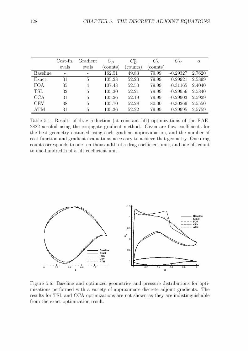
128 CHAPTER 5. THE DISCRETE ADJOINT EQUATIONS
Cost-fn. Gradient CD CvD CL CM α
evals evals (counts) (counts) (counts)Baseline - - 162.51 49.83 79.99 -0.29327 2.7620Exact 31 5 105.28 52.20 79.99 -0.29921 2.5899FOA 35 4 107.48 52.50 79.99 -0.31165 2.4040TSL 32 5 105.30 52.21 79.99 -0.29956 2.5840CCA 31 5 105.26 52.19 79.99 -0.29903 2.5929CEV 38 5 105.70 52.28 80.00 -0.30269 2.5550ATM 31 5 105.36 52.22 79.99 -0.29995 2.5759
Table 5.1: Results of drag reduction (at constant lift) optimizations of the RAE-2822 aerofoil using the conjugate gradient method. Given are flow coefficients forthe best geometry obtained using each gradient approximation, and the number ofcost-function and gradient evaluations necessary to achieve that geometry. One dragcount corresponds to one-ten thousandth of a drag coefficient unit, and one lift countto one-hundredth of a lift coefficient unit.
x0 0.2 0.4 0.6 0.8 1
BaselineExactFOACEVATM
x
c p
0 0.2 0.4 0.6 0.8 1
-1.5
-1
-0.5
0
0.5
1
BaselineExactFOACEVATM
Figure 5.6: Baseline and optimized geometries and pressure distributions for opti-mizations performed with a variety of approximate discrete adjoint gradients. Theresults for TSL and CCA optimizations are not shown as they are indistinguishablefrom the exact optimization result.
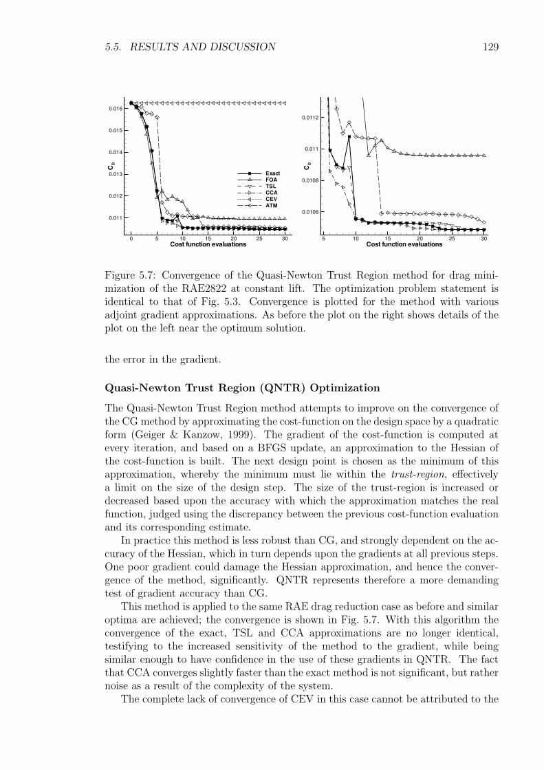
5.5. RESULTS AND DISCUSSION 129
Cost function evaluations
CD
0 5 10 15 20 25 30
0.011
0.012
0.013
0.014
0.015
0.016
ExactFOATSLCCACEVATM
Cost function evaluations
CD
5 10 15 20 25 30
0.0106
0.0108
0.011
0.0112
Figure 5.7: Convergence of the Quasi-Newton Trust Region method for drag mini-mization of the RAE2822 at constant lift. The optimization problem statement isidentical to that of Fig. 5.3. Convergence is plotted for the method with variousadjoint gradient approximations. As before the plot on the right shows details of theplot on the left near the optimum solution.
the error in the gradient.
Quasi-Newton Trust Region (QNTR) Optimization
The Quasi-Newton Trust Region method attempts to improve on the convergence ofthe CG method by approximating the cost-function on the design space by a quadraticform (Geiger & Kanzow, 1999). The gradient of the cost-function is computed atevery iteration, and based on a BFGS update, an approximation to the Hessian ofthe cost-function is built. The next design point is chosen as the minimum of thisapproximation, whereby the minimum must lie within the trust-region, effectivelya limit on the size of the design step. The size of the trust-region is increased ordecreased based upon the accuracy with which the approximation matches the realfunction, judged using the discrepancy between the previous cost-function evaluationand its corresponding estimate.
In practice this method is less robust than CG, and strongly dependent on the ac-curacy of the Hessian, which in turn depends upon the gradients at all previous steps.One poor gradient could damage the Hessian approximation, and hence the conver-gence of the method, significantly. QNTR represents therefore a more demandingtest of gradient accuracy than CG.
This method is applied to the same RAE drag reduction case as before and similaroptima are achieved; the convergence is shown in Fig. 5.7. With this algorithm theconvergence of the exact, TSL and CCA approximations are no longer identical,testifying to the increased sensitivity of the method to the gradient, while beingsimilar enough to have confidence in the use of these gradients in QNTR. The factthat CCA converges slightly faster than the exact method is not significant, but rathernoise as a result of the complexity of the system.
The complete lack of convergence of CEV in this case cannot be attributed to the
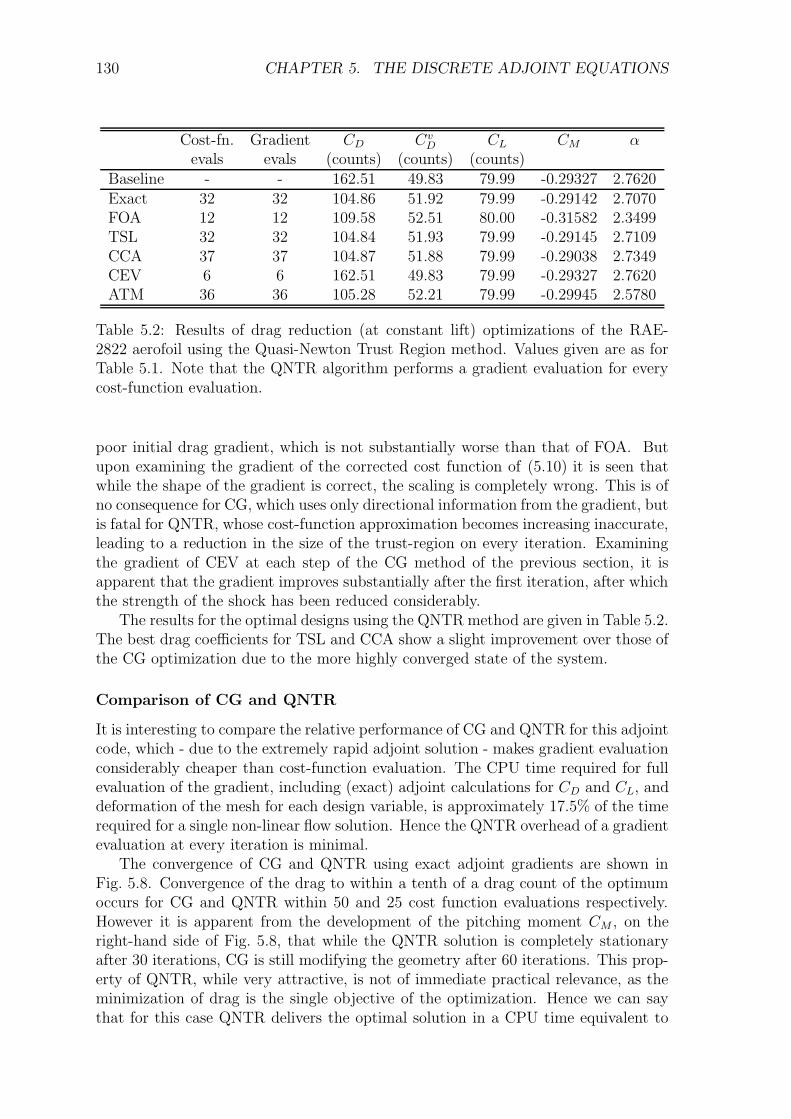
130 CHAPTER 5. THE DISCRETE ADJOINT EQUATIONS
Cost-fn. Gradient CD CvD CL CM α
evals evals (counts) (counts) (counts)Baseline - - 162.51 49.83 79.99 -0.29327 2.7620Exact 32 32 104.86 51.92 79.99 -0.29142 2.7070FOA 12 12 109.58 52.51 80.00 -0.31582 2.3499TSL 32 32 104.84 51.93 79.99 -0.29145 2.7109CCA 37 37 104.87 51.88 79.99 -0.29038 2.7349CEV 6 6 162.51 49.83 79.99 -0.29327 2.7620ATM 36 36 105.28 52.21 79.99 -0.29945 2.5780
Table 5.2: Results of drag reduction (at constant lift) optimizations of the RAE-2822 aerofoil using the Quasi-Newton Trust Region method. Values given are as forTable 5.1. Note that the QNTR algorithm performs a gradient evaluation for everycost-function evaluation.
poor initial drag gradient, which is not substantially worse than that of FOA. Butupon examining the gradient of the corrected cost function of (5.10) it is seen thatwhile the shape of the gradient is correct, the scaling is completely wrong. This is ofno consequence for CG, which uses only directional information from the gradient, butis fatal for QNTR, whose cost-function approximation becomes increasing inaccurate,leading to a reduction in the size of the trust-region on every iteration. Examiningthe gradient of CEV at each step of the CG method of the previous section, it isapparent that the gradient improves substantially after the first iteration, after whichthe strength of the shock has been reduced considerably.
The results for the optimal designs using the QNTR method are given in Table 5.2.The best drag coefficients for TSL and CCA show a slight improvement over those ofthe CG optimization due to the more highly converged state of the system.
Comparison of CG and QNTR
It is interesting to compare the relative performance of CG and QNTR for this adjointcode, which - due to the extremely rapid adjoint solution - makes gradient evaluationconsiderably cheaper than cost-function evaluation. The CPU time required for fullevaluation of the gradient, including (exact) adjoint calculations for CD and CL, anddeformation of the mesh for each design variable, is approximately 17.5% of the timerequired for a single non-linear flow solution. Hence the QNTR overhead of a gradientevaluation at every iteration is minimal.
The convergence of CG and QNTR using exact adjoint gradients are shown inFig. 5.8. Convergence of the drag to within a tenth of a drag count of the optimumoccurs for CG and QNTR within 50 and 25 cost function evaluations respectively.However it is apparent from the development of the pitching moment CM , on theright-hand side of Fig. 5.8, that while the QNTR solution is completely stationaryafter 30 iterations, CG is still modifying the geometry after 60 iterations. This prop-erty of QNTR, while very attractive, is not of immediate practical relevance, as theminimization of drag is the single objective of the optimization. Hence we can saythat for this case QNTR delivers the optimal solution in a CPU time equivalent to
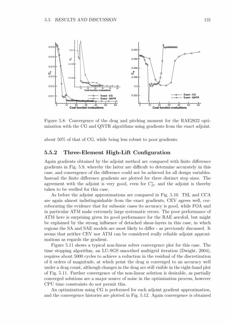
5.5. RESULTS AND DISCUSSION 131
Cost function evaluations
CD
0 10 20 30 40 50 60
0.011
0.012
0.013
0.014
0.015
0.016
Exact -CGExact -QNTR
Cost function evaluations
CD
10 20 30 40 50 60
0.0106
0.0108
0.011
Cost function evaluations
CM
0 10 20 30 40 50 60
-0.302
-0.3
-0.298
-0.296
-0.294
-0.292
Exact -CGExact -QNTR
Figure 5.8: Convergence of the drag and pitching moment for the RAE2822 opti-mization with the CG and QNTR algorithms using gradients from the exact adjoint.
about 50% of that of CG, while being less robust to poor gradients.
5.5.2 Three-Element High-Lift Configuration
Again gradients obtained by the adjoint method are compared with finite differencegradients in Fig. 5.9, whereby the latter are difficult to determine accurately in thiscase, and convergence of the difference could not be achieved for all design variables.Instead the finite difference gradients are plotted for three distinct step sizes. Theagreement with the adjoint is very good, even for Cv
D, and the adjoint is therebytaken to be verified for this case.
As before the adjoint approximations are compared in Fig. 5.10. TSL and CCAare again almost indistinguishable from the exact gradients, CEV agrees well, cor-roborating the evidence that for subsonic cases its accuracy is good, while FOA andin particular ATM make extremely large systematic errors. The poor performance ofATM here is surprising given its good performance for the RAE aerofoil, but mightbe explained by the strong influence of detached shear-layers in this case, in whichregions the SA and SAE models are most likely to differ - as previously discussed. Itseems that neither CEV nor ATM can be considered really reliable adjoint approxi-mations as regards the gradient.
Figure 5.11 shows a typical non-linear solver convergence plot for this case. Thetime stepping algorithm, an LU-SGS smoothed multigrid iteration (Dwight, 2004),requires about 5000 cycles to achieve a reduction in the residual of the discretizationof 6 orders of magnitude, at which point the drag is converged to an accuracy wellunder a drag count, although changes in the drag are still visible in the right-hand plotof Fig. 5.11. Further convergence of the non-linear solution is desirable, as partiallyconverged solutions are a major source of noise in the optimization process, howeverCPU time constraints do not permit this.
An optimization using CG is performed for each adjoint gradient approximation,and the convergence histories are plotted in Fig. 5.12. Again convergence is obtained
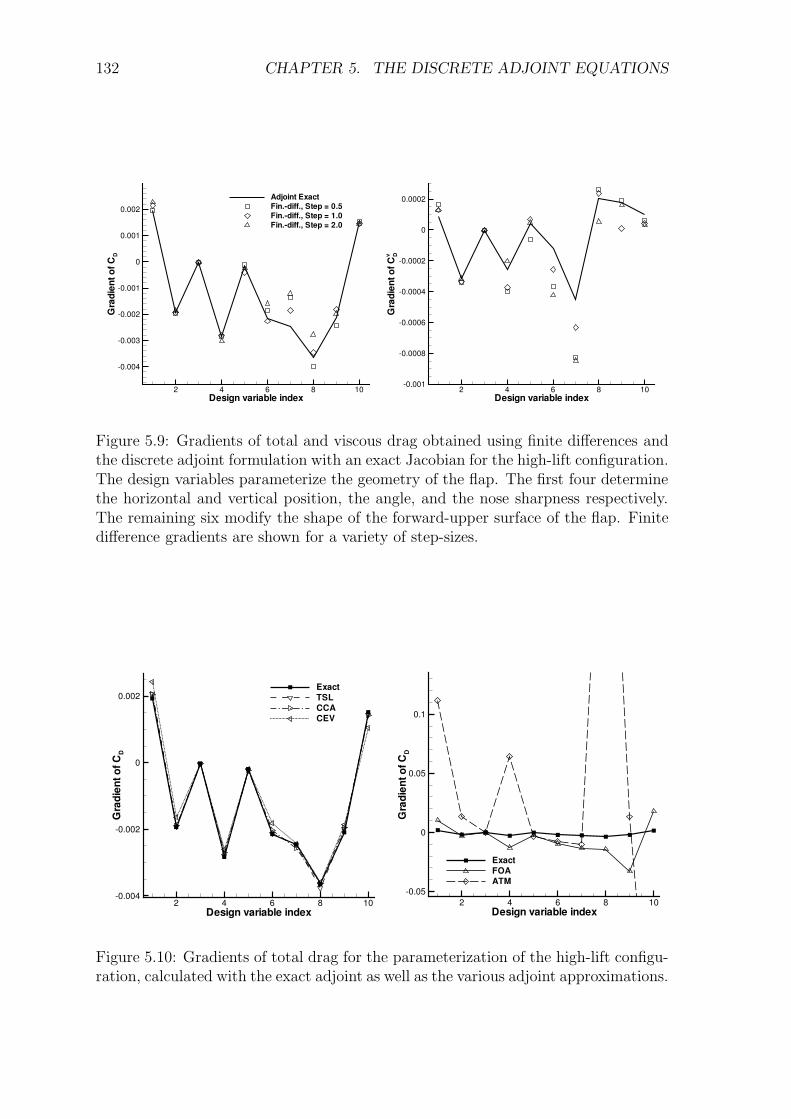
132 CHAPTER 5. THE DISCRETE ADJOINT EQUATIONS
Design variable index
Gra
dien
tofC
D
2 4 6 8 10
-0.004
-0.003
-0.002
-0.001
0
0.001
0.002
Adjoint ExactFin.-diff., Step = 0.5Fin.-diff., Step = 1.0Fin.-diff., Step = 2.0
Design variable indexG
radi
ento
fCDv
2 4 6 8 10-0.001
-0.0008
-0.0006
-0.0004
-0.0002
0
0.0002
Figure 5.9: Gradients of total and viscous drag obtained using finite differences andthe discrete adjoint formulation with an exact Jacobian for the high-lift configuration.The design variables parameterize the geometry of the flap. The first four determinethe horizontal and vertical position, the angle, and the nose sharpness respectively.The remaining six modify the shape of the forward-upper surface of the flap. Finitedifference gradients are shown for a variety of step-sizes.
Design variable index
Gra
dien
tofC
D
2 4 6 8 10-0.004
-0.002
0
0.002ExactTSLCCACEV
Design variable index
Gra
dien
tofC
D
2 4 6 8 10-0.05
0
0.05
0.1
ExactFOAATM
Figure 5.10: Gradients of total drag for the parameterization of the high-lift configu-ration, calculated with the exact adjoint as well as the various adjoint approximations.
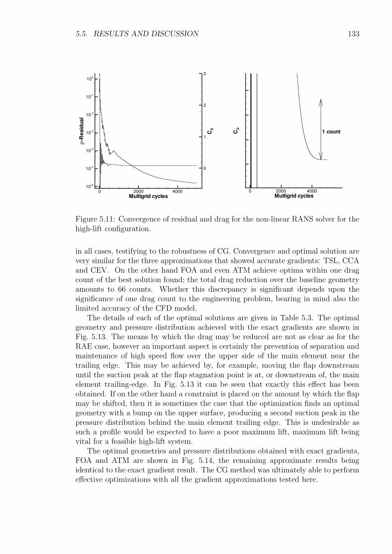
5.5. RESULTS AND DISCUSSION 133
Multigrid cycles
ρ-R
esid
ual
CD
0 2000 400010-6
10-5
10-4
10-3
10-2
10-1
100
0
1
2
3
Multigrid cycles
CD
0 2000 4000
1 count
Figure 5.11: Convergence of residual and drag for the non-linear RANS solver for thehigh-lift configuration.
in all cases, testifying to the robustness of CG. Convergence and optimal solution arevery similar for the three approximations that showed accurate gradients: TSL, CCAand CEV. On the other hand FOA and even ATM achieve optima within one dragcount of the best solution found; the total drag reduction over the baseline geometryamounts to 66 counts. Whether this discrepancy is significant depends upon thesignificance of one drag count to the engineering problem, bearing in mind also thelimited accuracy of the CFD model.
The details of each of the optimal solutions are given in Table 5.3. The optimalgeometry and pressure distribution achieved with the exact gradients are shown inFig. 5.13. The means by which the drag may be reduced are not as clear as for theRAE case, however an important aspect is certainly the prevention of separation andmaintenance of high speed flow over the upper side of the main element near thetrailing edge. This may be achieved by, for example, moving the flap downstreamuntil the suction peak at the flap stagnation point is at, or downstream of, the mainelement trailing-edge. In Fig. 5.13 it can be seen that exactly this effect has beenobtained. If on the other hand a constraint is placed on the amount by which the flapmay be shifted, then it is sometimes the case that the optimization finds an optimalgeometry with a bump on the upper surface, producing a second suction peak in thepressure distribution behind the main element trailing edge. This is undesirable assuch a profile would be expected to have a poor maximum lift, maximum lift beingvital for a feasible high-lift system.
The optimal geometries and pressure distributions obtained with exact gradients,FOA and ATM are shown in Fig. 5.14, the remaining approximate results beingidentical to the exact gradient result. The CG method was ultimately able to performeffective optimizations with all the gradient approximations tested here.
134 CHAPTER 5. THE DISCRETE ADJOINT EQUATIONS
Cost function evaluations
Nor
mal
ized
CD
0 10 20 30 40 50
0.92
0.94
0.96
0.98
1 ExactFOATSLCCACEVATM
Cost function evaluations
Nor
mal
ized
CD
10 15 20 25 30 35 40
0.918
0.9185
0.919
0.9195
0.92
0.9205
0.921
Figure 5.12: Convergence of the conjugate gradient algorithm for drag reductionat constant lift for the high-lift configuration, shown for optimizations based on alladjoint gradient approximations. As before convergence is plotted against non-linerRANS solver calls, thereby representing the approximate cost of the optimization.Symbols represent gradient evaluations, and the drag is normalized against the dragof the baseline geometry.
Cost-fn. Gradient ∆CD ∆CvD ∆CM ∆α
evals evals (counts) (counts)Baseline - - - - - -Exact 28 6 -66.68 -5.80 -0.0432 -0.587FOA 31 7 -65.76 -6.16 -0.0445 -0.518TSL 38 9 -66.68 -5.85 -0.0433 -0.582CCA 34 8 -66.69 -5.80 -0.0432 -0.587CEV 23 6 -66.66 -5.80 -0.0434 -0.584ATM 44 9 -65.59 -5.94 -0.0452 -0.509
Table 5.3: Results of drag reduction (at constant lift) optimizations of the high-liftconfiguration using the conjugate gradient method and a variety of adjoint gradientapproximations. Values given are changes in the coefficients, the coefficients them-selves are as in Table 5.1.
5.6. CONCLUSIONS 135
x
c p
-0.1 0 0.1 0.2 0.3 0.4 0.5 0.6 0.7 0.8 0.9 1 1.1 1.2
BaselineExact
∆cp=1
Figure 5.13: Baseline and optimized geometries and pressure distributions for dragminimization of the high-lift configuration with constant lift. The baseline angle ofattack is 9.61, whereas the optimized value is 9.02.
5.6 Conclusions
A method for construction and solution of the exact adjoint problem has been de-scribed which permits convergence within 5% of the CPU time for the non-linearproblem, and therefore typical full gradient calculations (including two adjoint so-lutions) within 20% of the time for a single non-linear problem solution. Memoryrequirements are however 6-7 times higher than the standard non-linear solver dueto the storage of the Jacobian, effectively limiting the method to 2d cases.
In an effort to reduce the memory requirements while maintaining the efficiencyof the method, several approximations to the discrete adjoint have been proposed andstudied with respect to optimizations on two 2d cases. Two of the approximationsstudied, TSL and CCA, showed consistently minimal variance from the exact gradi-ents, and as such may be used with confidence as substitutes for the exact adjointmethod. On the other hand it has been seen that approximating the adjoint of theturbulence model, either with constant eddy-viscosity (CEV) or the adjoint of a verysimilar model (ATM), leads to gradients that are good in some cases, but exception-ally poor in other cases. In particular CEV produced poor gradients for the RAEbaseline case with a strong shock but excellent gradients in the high-lift case; forATM the situation was reversed. These results suggest that construction of reliableadjoint method requires exact consideration of the particular turbulence model used.
Optimizations were performed with the conjugate gradient (CG) algorithm, whichconverged reasonably well for all cases and with all gradients, no matter how poor.
136 CHAPTER 5. THE DISCRETE ADJOINT EQUATIONS
x
c p
0.8 0.9 1 1.1
BaselineExactFOAATM
∆cp=1
Figure 5.14: Baseline and optimized geometries and pressure distributions for the flapof the high-lift configuration, from optimizations performed with a variety of approx-imate discrete adjoint gradients. The results for TSL, CCA and CEV optimizationsare not shown as they are indistinguishable from the exact optimization result.
5.6. CONCLUSIONS 137
Optimal results obtained with variously inaccurate gradients resulted in optimal so-lutions differing by no more than 2.5 drag counts for the RAE case and 1 drag countfor the high-lift case. A consequence is that an extremely poor (and correspondinglycheap) adjoint approximation, such as FOA, could be useful in situations where highaccuracy is not required.
It has also been shown that the possibility for rapid gradient evaluation allowsefficient use of the Quasi-Newton Trust-Region method, which can reduce the overalloptimization time by 50% in comparison to CG, whereby the method is much moresensitive to poor gradients.
Based on the results of this study an adjoint solver using the CCA approximationwill be further developed, and a reduction in memory requirements to about threetimes those of the non-linear solver are expected.
Chapter 6
Conclusions
A complete unstructured grid finite volume method for the RANS equations was pre-sented in Chapter 2, including all details of the JST convective flux discretization,boundary conditions and turbulence models, as implemented in the flow solver theDLR-TAU-Code. In addition the exact and some approximations of the Jacobian ofthe complete spatial discretization were derived and implemented, of which selectedparts were described. In particular the full Jacobian of the JST convective flux wasderived, and an approximation is proposed (namely the regarding of the coefficient ofdissipation as constant) which simplifies the expression for the Jacobian significantly.It was shown that the terms in the derivative neglected through this approxima-tion were of higher order in the grid-spacing ∆x than the remaining terms, therebyproviding an original justification for this approximation. Further, a method for thetreatment in the Jacobian of strongly implemented boundary conditions was detailed.
The implicit solution of the discretized equations was considered next in Chap-ter 3. It was shown, based on the practical example of a novel formulation of theLU-SGS scheme with FAS multigrid, that it is possible to construct an efficient, ap-proximately factored, implicit method that has identical memory requirements to thestandard explicit Runge-Kutta scheme. The method is also cheaper in terms of CPUtime per iteration than said scheme. Even so it is able to operate with CFL numbersof the order of 1000 for Euler flow problems, and of the order of 10 for complex 3dhigh-Reynolds number Navier-Stokes problems, for which it converges in 50%–90%of the iteration count of RK. Finally the scheme is at least as stable in a wide rangeof situations as RK, and can therefore be used as a true slot-in replacement for thatscheme in all situations. The method has been implemented in the TAU-Code andat time of writing is widely used within the European aerospace industry.
While the final assessment of the performance of LU-SGS was based on the nu-merical investigation of the method applied to practical engineering test-cases, theproperties of the scheme were also examined in the context of diagonal dominance ofthe implicit matrix, and Fourier analysis. It has been shown by numerical comparisonwith related schemes designed to be diagonally dominant, that diagonal dominanceis not desirable in terms of non-linear convergence. Fourier analysis of the schemewas unsuccessful in that results fundamentally disagreed with numerical observa-tions, the cause of which was traced back to the oversimplified model of the implicitmethod necessitated by the linear nature of the model equation under consideration.
138
139
Nonetheless these investigations were instrumental in formulating and understand-ing the LU-SGS scheme. Last, but not least, the time-accuracy of the scheme wasexamined.
By relaxing the constraint that the memory requirements of the scheme should notbe significantly greater than those of Runge-Kutta, explicit storage of the Jacobian,and the subsequent solution via Krylov methods became possible, investigated inChapter 4. An exact Newton method based on the explicitly stored Jacobian of asecond-order central discretization was examined. Solution of the linear system ateach step using the existing non-linear time stepping method was investigated. It wasshown both theoretically, and on the basis of a turbulent test case, that the resultinglinear system convergence is identical to the asymptotic convergence of the non-lineariteration using the same method. However this approach was ultimately found to beinappropriate as part of a Newton method due to its instability for Jacobians basedon partially-converged non-linear solutions.
Attention was therefore turned to Krylov methods, which provided convergencein all cases given sufficient preconditioning. However, it was found that the levelof preconditioning needed was often excessive. For a simple 2d turbulent test casean ILU(4) preconditioner and a GMRES(50) method was required. The resultingalgorithm required about 15 times more memory than the standard solver, which wasconsidered an unacceptable overhead.
Attention was therefore turned to Jacobians based on first-order fluxes, and twomethods were proposed, one using a Gauss-Seidel inner iteration (FOGSI), and oneusing an ILU preconditioned Krylov method (FOKI). In FOKI the turbulence equa-tion iteration was completely separated from the mean flow iteration, and this wasseen to save memory, as well as improve the convergence of the method. FOKI wasshown to be 4-5 times faster than LU-SGS for the cases considered, while the result-ing code required about 5 times more memory. The method was seen to be a verypromising candidate for further development, in particular in terms of extension tocomplex three-dimensional configurations.
These investigations, covering a wide range of Jacobian approximations and linearsolvers, provided insights into the relationship between the two critical elements ofan implicit scheme. In particular the importance of proper consideration of boundaryconditions, even in poor Jacobians, and aspects of the trade-off between linear andnon-linear stiffness were demonstrated.
The effort required to evaluate the Jacobian for the exact Newton method of theprevious chapter, which amounts to a linearization of the entire discrete flow solver,suggested looking for alternative applications. The adjoint method, in Chapter 5, wasseen to be such an application which allows the rapid evaluation of the derivatives of aflow quantity, such as drag, with respect to some design variables which parameterizethe aerodynamic shape. These derivatives are then used for gradient-based shapeoptimization.
The adjoint method suffered under similar problems to the exact Newton methodhowever: considerable storage was required and the resulting linear system was dif-ficult to solve. Using a simplified Jacobian affected the accuracy of the resultinggradients, unlike in the Newton method where it only affected the transient conver-gence behaviour. The sensitivity of the gradients to approximations of the Jacobianwas therefore examined on the basis of two optimization test cases. It was seen
140 CHAPTER 6. CONCLUSIONS
that considerable simplifications were possible, without significant modifications tothe optimum, and these differences were quantified. Thereby greater understandingof the sensitivity of the optimization to inaccurate gradients, and in particular toapproximations of the adjoint equations was won.
6.1 Further Work
This thesis does not represent the last word on the methods discussed; rather it ispart of a continuing investigation, especially in the case of the adjoint method, andit is hoped that the results herein will inform and guide future work.
While the LU-SGS method is more-or-less complete, the FOKI approach has sofar only been shown for two-dimensional test cases. If it to be applied routinely topractical cases it must be made at least as robust as LU-SGS and Runge-Kutta forcomplex geometries, poor grids, and flows with separation. Additionally the area ofstart-up methods should be investigated, including consideration of when it is possibleto start the full method and expect convergence. For these questions more experiencewith the approach is needed in practice.
The principal defect of the discrete adjoint algorithm as described here is its largememory requirements in relation to the non-linear solver, which are a consequence ofthe explicit storage of the Jacobian and the use of ILU preconditioned GMRES. It isexpected that in the near future an accompanying adjoint solver will be demanded ofany industrially applied computational aerodynamics code, not only for the purposesof optimization, but also for error estimation and goal-based mesh adaptation. In thiscase the memory performance of the adjoint solver must be improved significantly ifit is to enjoy routine use.
The path to this goal is highlighted by the investigations of Chapter 5, whichshow that given some approximations which have little effect on the adjoint solution,the construction of the adjoint residual can be simplified and accelerated consid-erably, while the associated memory requirements are also reduced, see especiallySection 5.4.3. Future work will concern the implementation of this formulation of theresidual in an efficient manner.
Apart from its high memory requirements, the ILU preconditioner may not longerbe used, as the Jacobian is not available explicitly. Instead solution using existingtime stepping methods for the non-linear equation will be applied, as was done for thelinear problem in Section 4.3.1. This approach had two nice properties: guaranteedconvergence of the linear system given convergence of the non-linear system, as wellas identical asymptotic convergence rate. If these are to be preserved for the adjointequation, the time stepping scheme must also be “adjointed” (Giles, 2001). This willbe done, and it is expected that the resulting system will have similar stability andconvergence properties and similar memory requirements to the non-linear solver.
Given the adjoint approach, the operation that now dominates the cost of angradient evaluation is the deformation of the grid for each design variable, in orderto find the mesh sensitivities. It was shown how this cost may be eliminated inSection 5.3.3, and work is progressing to implement this approach, whereby the mosteffort needs to be expended in the linearization of the mesh deformation algorithm,and the evaluation of the terms ∂R/∂X and ∂I/∂X by hand.
With these tools complete the gradient-based optimization of a three-dimensional

6.1. FURTHER WORK 141
wing-body configuration with a mesh of several million points and a parameterizationof 100− 1000 design variables should be possible in well under one day’s computingtime on a small PC cluster, and this specific calculation is the immediate goal.
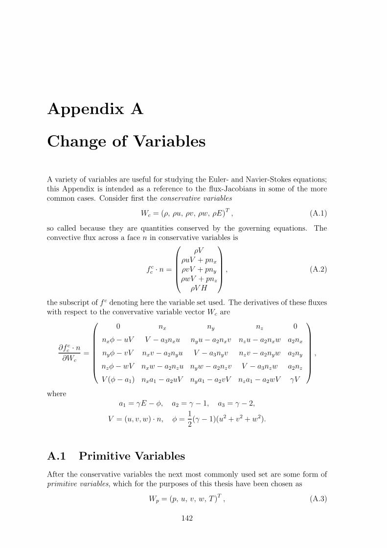
Appendix A
Change of Variables
A variety of variables are useful for studying the Euler- and Navier-Stokes equations;this Appendix is intended as a reference to the flux-Jacobians in some of the morecommon cases. Consider first the conservative variables
Wc = (ρ, ρu, ρv, ρw, ρE)T , (A.1)
so called because they are quantities conserved by the governing equations. Theconvective flux across a face n in conservative variables is
f cc · n =
ρVρuV + pnxρvV + pnyρwV + pnzρV H
, (A.2)
the subscript of f c denoting here the variable set used. The derivatives of these fluxeswith respect to the convervative variable vector Wc are
∂f cc · n∂Wc
=
0 nx ny nz 0
nxφ− uV V − a3nxu nyu− a2nxv nzu− a2nxw a2nx
nyφ− vV nxv − a2nyu V − a3nyv nzv − a2nyw a2ny
nzφ− wV nxw − a2nzu nyw − a2nzv V − a3nzw a2nz
V (φ− a1) nxa1 − a2uV nya1 − a2vV nza1 − a2wV γV
,
wherea1 = γE − φ, a2 = γ − 1, a3 = γ − 2,
V = (u, v, w) · n, φ =1
2(γ − 1)(u2 + v2 + w2).
A.1 Primitive Variables
After the conservative variables the next most commonly used set are some form ofprimitive variables, which for the purposes of this thesis have been chosen as
Wp = (p, u, v, w, T )T , (A.3)
142
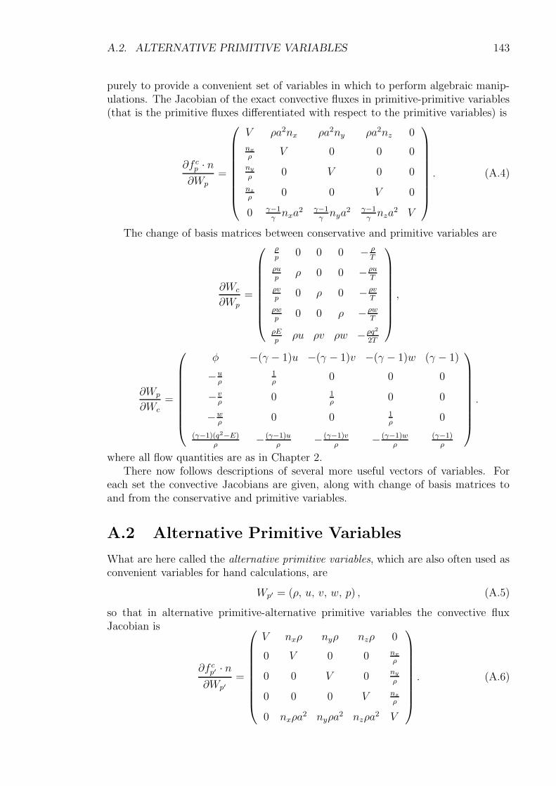
A.2. ALTERNATIVE PRIMITIVE VARIABLES 143
purely to provide a convenient set of variables in which to perform algebraic manip-ulations. The Jacobian of the exact convective fluxes in primitive-primitive variables(that is the primitive fluxes differentiated with respect to the primitive variables) is
∂f cp · n∂Wp
=
V ρa2nx ρa2ny ρa2nz 0
nxρ
V 0 0 0
nyρ
0 V 0 0
nzρ
0 0 V 0
0 γ−1γnxa
2 γ−1γnya
2 γ−1γnza
2 V
. (A.4)
The change of basis matrices between conservative and primitive variables are
∂Wc
∂Wp
=
ρp
0 0 0 − ρT
ρup
ρ 0 0 −ρuT
ρvp
0 ρ 0 −ρvT
ρwp
0 0 ρ −ρwT
ρEp
ρu ρv ρw −ρq2
2T
,
∂Wp
∂Wc=
φ −(γ − 1)u −(γ − 1)v −(γ − 1)w (γ − 1)
−uρ
1ρ
0 0 0
−vρ
0 1ρ
0 0
−wρ
0 0 1ρ
0
(γ−1)(q2−E)ρ
− (γ−1)uρ
− (γ−1)vρ
− (γ−1)wρ
(γ−1)ρ
.
where all flow quantities are as in Chapter 2.There now follows descriptions of several more useful vectors of variables. For
each set the convective Jacobians are given, along with change of basis matrices toand from the conservative and primitive variables.
A.2 Alternative Primitive Variables
What are here called the alternative primitive variables, which are also often used asconvenient variables for hand calculations, are
Wp′ = (ρ, u, v, w, p) , (A.5)
so that in alternative primitive-alternative primitive variables the convective fluxJacobian is
∂f cp′ · n∂Wp′
=
V nxρ nyρ nzρ 0
0 V 0 0 nxρ
0 0 V 0 nyρ
0 0 0 V nzρ
0 nxρa2 nyρa
2 nzρa2 V
. (A.6)
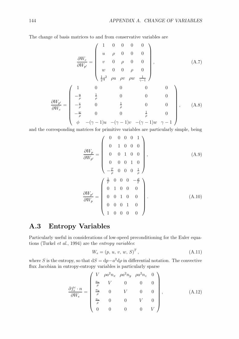
144 APPENDIX A. CHANGE OF VARIABLES
The change of basis matrices to and from conservative variables are
∂Wc
∂Wp′=
1 0 0 0 0
u ρ 0 0 0
v 0 ρ 0 0
w 0 0 ρ 0
12q2 ρu ρv ρw 1
γ−1
, (A.7)
∂Wp′
∂Wc=
1 0 0 0 0
−uρ
1ρ
0 0 0
−vρ
0 1ρ
0 0
−wρ
0 0 1ρ
0
φ −(γ − 1)u −(γ − 1)v −(γ − 1)w γ − 1
, (A.8)
and the corresponding matrices for primitive variables are particularly simple, being
∂Wp
∂Wp′=
0 0 0 0 1
0 1 0 0 0
0 0 1 0 0
0 0 0 1 0
−Tρ
0 0 0 1ρ
, (A.9)
∂Wp′
∂Wp=
1T
0 0 0 − ρT
0 1 0 0 0
0 0 1 0 0
0 0 0 1 0
1 0 0 0 0
. (A.10)
A.3 Entropy Variables
Particularly useful in considerations of low-speed preconditioning for the Euler equa-tions (Turkel et al., 1994) are the entropy variables:
We = (p, u, v, w, S)T , (A.11)
where S is the entropy, so that dS = dp−a2dρ in differential notation. The convectiveflux Jacobian in entropy-entropy variables is particularly sparse
∂f ce · n∂We
=
V ρa2nx ρa2ny ρa2nz 0
nxρ
V 0 0 0
nyρ
0 V 0 0
nzρ
0 0 V 0
0 0 0 0 V
, (A.12)
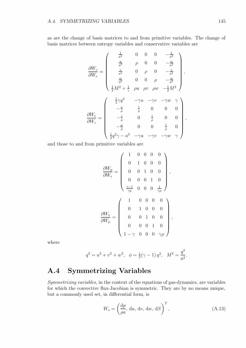
A.4. SYMMETRIZING VARIABLES 145
as are the change of basis matrices to and from primitive variables. The change ofbasis matrices between entropy variables and conservative variables are
∂Wc
∂We=
1a2 0 0 0 − 1
a2
ua2 ρ 0 0 − u
a2
va2 0 ρ 0 − v
a2
wa2 0 0 ρ − w
a2
12M2 + 1
γρu ρv ρw − 1
2M2
,
∂We
∂Wc
=
12γq2 −γu −γv −γw γ
−uρ
1ρ
0 0 0
−vρ
0 1ρ
0 0
−wρ
0 0 1ρ
0
12q2γ − a2 −γu −γv −γw γ
,
and those to and from primitive variables are
∂Wp
∂We
=
1 0 0 0 0
0 1 0 0 0
0 0 1 0 0
0 0 0 1 0
γ−1γρ
0 0 0 1γρ
,
∂We
∂Wp
=
1 0 0 0 0
0 1 0 0 0
0 0 1 0 0
0 0 0 1 0
1− γ 0 0 0 γρ
,
where
q2 = u2 + v2 + w2, φ = 12(γ − 1) q2, M2 =
q2
a2.
A.4 Symmetrizing Variables
Symmetrizing variables, in the context of the equations of gas-dynamics, are variablesfor which the convective flux-Jacobian is symmetric. They are by no means unique,but a commonly used set, in differential form, is
Ws =
(dp
ρa, du, dv, dw, dS
)T, (A.13)
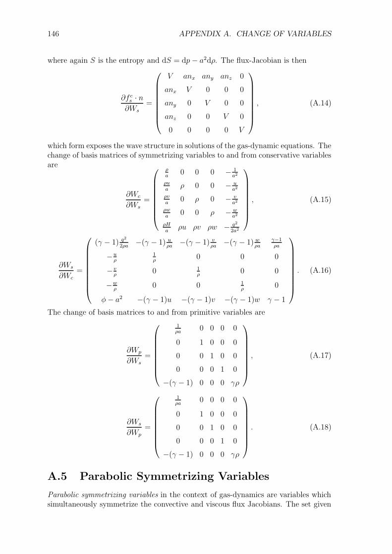
146 APPENDIX A. CHANGE OF VARIABLES
where again S is the entropy and dS = dp− a2dρ. The flux-Jacobian is then
∂f cs · n∂Ws
=
V anx any anz 0
anx V 0 0 0
any 0 V 0 0
anz 0 0 V 0
0 0 0 0 V
, (A.14)
which form exposes the wave structure in solutions of the gas-dynamic equations. Thechange of basis matrices of symmetrizing variables to and from conservative variablesare
∂Wc
∂Ws=
ρa
0 0 0 − 1a2
ρua
ρ 0 0 − ua2
ρva
0 ρ 0 − va2
ρwa
0 0 ρ − wa2
ρHa
ρu ρv ρw − q2
2a2
, (A.15)
∂Ws
∂Wc
=
(γ − 1) q2
2ρa−(γ − 1) u
ρa−(γ − 1) v
ρa−(γ − 1) w
ρaγ−1ρa
−uρ
1ρ
0 0 0
−vρ
0 1ρ
0 0
−wρ
0 0 1ρ
0
φ− a2 −(γ − 1)u −(γ − 1)v −(γ − 1)w γ − 1
. (A.16)
The change of basis matrices to and from primitive variables are
∂Wp
∂Ws=
1ρa
0 0 0 0
0 1 0 0 0
0 0 1 0 0
0 0 0 1 0
−(γ − 1) 0 0 0 γρ
, (A.17)
∂Ws
∂Wp
=
1ρa
0 0 0 0
0 1 0 0 0
0 0 1 0 0
0 0 0 1 0
−(γ − 1) 0 0 0 γρ
. (A.18)
A.5 Parabolic Symmetrizing Variables
Parabolic symmetrizing variables in the context of gas-dynamics are variables whichsimultaneously symmetrize the convective and viscous flux Jacobians. The set given
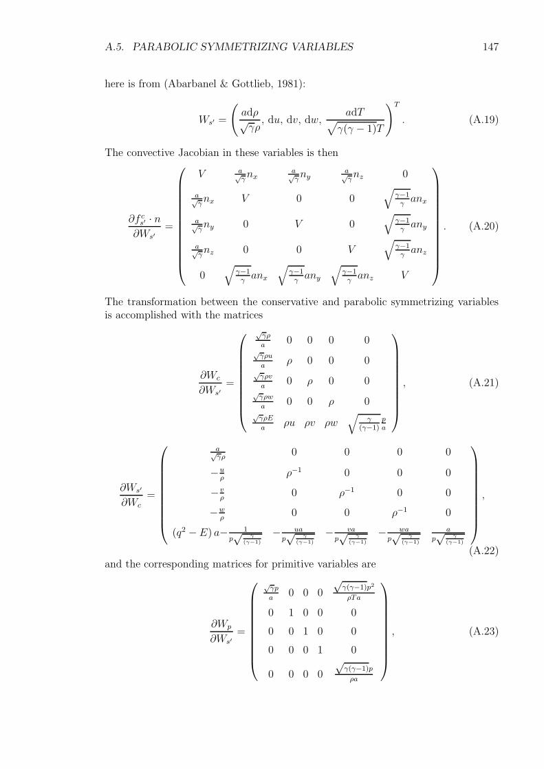
A.5. PARABOLIC SYMMETRIZING VARIABLES 147
here is from (Abarbanel & Gottlieb, 1981):
Ws′ =
(adρ√γρ, du, dv, dw,
adT√γ(γ − 1)T
)T
. (A.19)
The convective Jacobian in these variables is then
∂f cs′ · n∂Ws′
=
V a√γnx
a√γny
a√γnz 0
a√γnx V 0 0
√γ−1γanx
a√γny 0 V 0
√γ−1γany
a√γnz 0 0 V
√γ−1γanz
0√
γ−1γanx
√γ−1γany
√γ−1γanz V
. (A.20)
The transformation between the conservative and parabolic symmetrizing variablesis accomplished with the matrices
∂Wc
∂Ws′=
√γρ
a0 0 0 0
√γρu
aρ 0 0 0
√γρv
a0 ρ 0 0
√γρw
a0 0 ρ 0
√γρE
aρu ρv ρw
√γ
(γ−1)pa
, (A.21)
∂Ws′
∂Wc
=
a√γρ
0 0 0 0
−uρ
ρ−1 0 0 0
−vρ
0 ρ−1 0 0
−wρ
0 0 ρ−1 0
(q2 − E) a− 1
p√
γ(γ−1)
− ua
p√
γ(γ−1)
− va
p√
γ(γ−1)
− wa
p√
γ(γ−1)
a
p√
γ(γ−1)
,
(A.22)and the corresponding matrices for primitive variables are
∂Wp
∂Ws′=
√γp
a0 0 0
√γ(γ−1)p2
ρTa
0 1 0 0 0
0 0 1 0 0
0 0 0 1 0
0 0 0 0
√γ(γ−1)p
ρa
, (A.23)
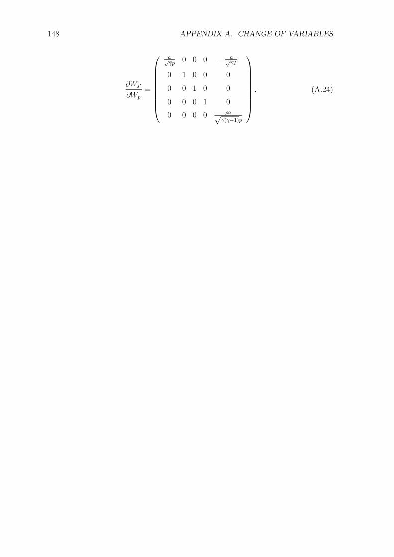
148 APPENDIX A. CHANGE OF VARIABLES
∂Ws′
∂Wp=
a√γp
0 0 0 − a√γT
0 1 0 0 0
0 0 1 0 0
0 0 0 1 0
0 0 0 0 ρa√γ(γ−1)p
. (A.24)
References
Abarbanel, S., & Gottlieb, D. 1981. Optimal Time Splitting for Two- and Three-Dimensional Navier-Stokes Equations with Mixed Derivatives. Journal of Com-putational Physics, 41, 1–33.
Badcock, K., Woodgate, M., Cantariti, F., & Richards, B. 1999. Solution of the Un-steady Euler Equations in Three Dimensions Using a Fully Unfactored Method.Glasgow University, Department of Aerospace Engineering, Technical Report9909.
Balay, S., Gropp, W.D., Curfman-McInnes, L., & Smith, B.F. 1997. Efficient Man-agement of Parallelism in Object Oriented Numerical Software Libraries. Pages163–202 of: Arge, E., Bruaset, A. M., & Langtangen, H. P. (eds), Modern Soft-ware Tools in Scientific Computing. Birkhauser Press.
Balay, S., Buschelman, K., Eijkhout, V., Gropp, W.D., Kaushik, D., Knepley, M.G.,Curfman-McInnes, L., Smith, B.F., & Zhang, H. 2004. PETSc Users Manual.Tech. rept. ANL-95/11 - Revision 2.1.5. Argonne National Laboratory.
Balay, S., Buschelman, K., Gropp, W.D., Kaushik, D., Knepley, M.G., Curfman-McInnes, L., Smith, B.F., & Zhang, H. 2006. PETSc Web page. http://www.-mcs.anl.gov/petsc.
Bhatia, R. 1997. Matrix Analysis. Springer. ISBN 0-387-94846-5.
Blazek, J. 1993. Investigations of the Implicit LU-SSOR Scheme. DLR Forschungs-bericht, DLR-FB-93/51.
Blazek, J. 2001. Computational Fluid Dynamics: Principles and Applications. Else-vier Science. ISBN 0-08-043009-0.
Boussinesq, J. 1877. Theorie de l’Ecoulement Tourbillonant. Comptes-Rendus del’Academie les Sciences, 23, 46–50.
Brezillon, J., & Dwight, R.P. 2005. Discrete Adjoint of the Navier-Stokes Equaitonsfor Aerodynamic Shape Optimization. Evolutionary and Deterministic Methodsfor Design, EUROGEN.
Brezillon, J., & Gauger, N.R. 2004. 2D and 3D Aerodynamic Shape OptimizationUsing the Adjoint Aproach. Aerospace Science and Technology Journal, 8(8),715–727.
149
150 REFERENCES
Brezillon, J., & Wild, J. 2005. Evaluation of Different Optimization Strategies forthe Design of a High-Lift Flap Device. EUROGEN 2005, Munich, September.
Burdyshaw, C., & Anderson, W. 2005. A General and Extensible Unstructured MeshAdjoint Method. 43th AIAA Aerospace Sciences Meeting and Exhibit, January10-13, Reno, NV., AIAA-2005-0335.
Butcher, J. C. 1987. The numerical analysis of ordinary differential equations: Runge-Kutta and general linear methods. Wiley-Interscience.
Cai, X.-C., Gropp, W.D., Keyes, D.E., & Tidriri, M.D. 1995. Newton-Krylov-Schwarzmethods in CFD. Proceedings of the International Workshop on Numerical Meth-ods for the Navier-Stokes Equations, Vieweg, Braunschweig, 17–30.
Campobasso, M.S., & Giles, M.B. 2002. Effects of Flow Instabilities on the LinearAnalysis of Turbomachinery Aeroelasticity. Proceedings of 38th Joint PropulsionConference and Exhibit, Indianapolis,AIAA-2002-4085.
Campobasso, M.S., & Giles, M.B. 2004. Stabilization of a linear flow solver for tur-bomachinery aeroelasticity by means of the recursive projection method. AIAAJournal, 42(9), 1765–1774.
Cantariti, F., Dubuc, L., Gribben, B., Woodgate, M., Badcock, K., & Richards, B.1997. Approximate Jacobians for the Solution of the Euler and Navier-StokesEquations. Glasgow University, Department of Aerospace Engineering, TechnicalReport 9705.
Cantariti, F., Woodgate, M., Badcock, K., & Richards, B. 1999. Solution of theNavier-Stokes Equations in Three Dimensions Using a Fully Unfactored Method.Glasgow University, Department of Aerospace Engineering, Technical Report9908.
Castro, C., Lozano, C., Palacios, F., & Zuazua, E. 2006. A Systematic ContinuousAdjoint Approach to Viscous Aerodynamic Design on Unstructured Grids. 44thAIAA ASM Conference, Reno, NV. AIAA-2006-0051.
Chisholm, T., & Zingg, D.W. 2002. A Fully Coupled Newton-Krylov Solver forTurbulent Aerodynamic Flows. ICAS 2002 Conference, Toroto, Paper 333.
Cook, P.H., McDonald, M.A., & Firmin, M.C.P. 1979. Aerofoil RAE 2822 — Pres-sure Distributions and Boundary Layer and Wake Measurements. AGARD–AR,no. 138. Neuilly-sur-Seine, France: AGARD — Advisory Group for AerospaceResearch & Development. Chap. 6.
Dubuc, L., Badcock, K., Richards, B., & Woodgate, M. 1996. Implicit Navier-Stokessimulations of unsteady flows. Proceedings of R.Ae.Soc Conference in UnsteadyAerodynamics, London.
Dwight, R.P. 2004. Application of Approximately Factored Implicit Schemes toUnsteady Navier-Stokes Calculations. Proceedings of the ICCFD3 Conference,Toronto, Springer.
REFERENCES 151
Dwight, R.P., & Brezillon, J. 2006. Effect of Various Approximations of the Dis-crete Adjoint on Gradient-Based Optimization. Proceedings of the 44th AIAAAerospace Sciences Meeting and Exhibit, Reno NV. AIAA-2006-0690.
Edwards, J.R., & Chandra, S. 1996. Comparison of Eddy-Viscosity Transport Turbu-lence Models for Three-Dimensional Shock-Seperated Flowfields. AIAA Journal,34(4).
Faßbender, J. 2003. Improved Robustness for Numerical Simulations of TurbulentFlows around Civil Transport Aircraft at Flight Reynolds Numbers. Ph.D. thesis,Institute of Aerodynamics and Flow Technology, DLR, Brauschweig.
Feingold, D.G., & Varga, R.S. 1962. Block Diagonally Dominant Matrices and Gen-eralizations of the Gerschgorin Circle Theorem. Pacific J. Math., 12, 1241–1250.
Galle, M. 1995. Solution of the Euler and Navier-Stokes Equations of Hybrid Grids.AGARD-CP-578, 31.1–31.9.
Galle, M. 1999. Ein Verfahren zur numerischen Simulation kompressibler, reibungs-behafteter Stromungen auf hybriden Netzen. DLR Forschungsbericht, DLR-FB-99/04.
Gauger, N., & Brezillon, J. 2003. Aerodynamic shape optimization using the adjointmethod. Journal of the Aeronautical Society of India, 54(3).
Geiger, & Kanzow. 1999. Numerische Verfarhren zur Loesung unrestringierter Opti-mierungsaufgaben. Springer.
Gerhold, T., Galle, M., Friedrich, O., & Evans, J. 1997. Calculation of Complex 3DConfigurations Employing the DLR TAU-Code. AIAA Paper, AIAA-97-0167.
Giles, M.B. 2001. On the iterative solution of adjoint equations. Automatic Differ-entiation: From Simulation to Optimization, 145–152.
Giles, M.B., Duta, M.C., Muller, J.D., & Pierce, N.A. 2003. Algorithm Developmentsfor Discrete Adjoint Methods. AIAA Journal, 41(2), 198–205.
Glowinski, R., & Pironneau, O. 1975. On the Numerical Compuation of the Minimum-Drag Profile in Laminar Flow. Journal of Fluid Mechanics, 72, 385–389.
Griewank, A., & Walther, A. 2002. On Constrained Optimization by Adjoint BasedQuasi-Newton Methods. Optimization Methods and Software, 17(5), 869–889.
Griewank, Andreas. 2000. Evaluating Derivatives, Principles and Techniques of Algo-rithmic Differentiation. Number 19 in Frontiers in Appl. Math. SIAM, Philadel-phia. ISBN 0898714516.
Hicks, R.M., & Henne, P.A. 1978. Wing Design by Numerical Optimization. Journalof Aircraft, 15, 407–412.
Hirsch, C. 1989. Numerical Computation of Internal and External Flows: Funda-mentals of Numerical Discretization v. 1. John Wiley and Sons Ltd. ISBN0471923850.
152 REFERENCES
Jameson, A. 1988. Aerodynamic Design Via Control Theory. Journal of ScientificComputing, 3, 233–260.
Jameson, A. 1991. Time dependant calculations using multigrid with applications tounsteady flows past airfoils and wings. AIAA Paper.
Jameson, A. 1995. Analysis and design of numerical schemes for gas dynamics I:artificial diffusion, upwind biasing, limiters and their effect on accuracy andmultigrid convergence. International Journal of Computational Fluid Dynamics,4(171).
Jameson, A., & Baker, T. 1984. Multigrid Solution of the Euler Equations for AircraftConfigurations. AIAA Paper, AIAA-84-0093.
Jameson, A., & Caughey, D.A. 2001. How Many Steps are Required to Solve theEuler Equations of Steady Compressible Flow: In Search of a Fast SolutionAlgorithm. 15th AIAA Computational Fluid Dynamics Conference, June 11-14,2001, Anaheim, CA.
Jameson, A., & Turkel, E. 1981. Implicit schemes and LU-decompositions. Mathe-matics of Computation, 37, 385–397.
Jameson, A., Schmidt, W., & Turkel, E. 1981. Numerical Solutions of the Euler Equa-tions by Finite Volume Methods Using Runge-Kutta Time-Stepping Schemes.AIAA Paper. AIAA-81-1259.
Johnson, F., Tinoco, E., & Yu, N. 2003. Thirty Years of Development and Applicationof CFD at Boeing Commercial Airplanes, Seattle. 16th AIAA CFD Conference,Orlando, Florida.
Kim, C.S., Kim, C., & O.H., Rho. 2003. Feasibility Study of the Constant Eddy Vis-cosity Assumption in Gradient-Based Design Optimization. Journal of Aircraft,40, 1168–1176.
Kim, S., Alonso, J., & Jameson, A. 2002. Design Optimization of High-Lift Con-figurations Using a Viscous Continuous Adjoint Method. 40th AIAA AerospaceSciences Meeting and Exhibit, Reno. AIAA-2002-0844.
Knoll, D.A., & Keyes, D.E. 2004. Jacobian-free Newton-Krylov Methods: A Survey ofApproaches and Applications. Journal of Computational Physics, 193, 357–397.
Kroll, N., & Fassbender, J. K. (eds). 2005. MEGAFLOW — Numerical Flow Sim-ulation for Aircraft Design: Results of the second phase of the German CFDinitiative MEGAFLOW presented during its closing symposium at DLR, Braun-schweig, Germany, December 10th and 11th 2002. Notes on Numerical FluidMechanics and Multidisciplinary Design, vol. 89. Berlin: Springer Verlag.
Kroll, N., Gauger, N.R., Brezillon, J., Becker, K., & Schulz, V. 2004. OngoingActivities in Shape Optimization within the German Project MEGADESIGN.ECCOMAS Finland, 24-28 July.
REFERENCES 153
Le Chuiton, F. 2004. On the Non-Dimensionalization of the Navier-Stokes equations.DLR Institutsbericht, AS. IB 124-2004/10.
Lohner, R., & Galle, M. 2002. Minimization of Indirect Addressing for Edge-BasedField Solvers. 40th AIAA Aerospace Sciences Meeting and Exhibit, January 14-17, Reno, NV.
Lohner, R., Soto, O., & Yang, Chi. 2003. An Adjoint-Based Design Methodology forCFD Optimization Problems. AIAA Paper, AIAA-03-0299.
Luo, H., Baum, J.D., & Lohner, R. 1998. A Fast, Matrix-Free Implicit Method forCompressible Flows on Unstructured Grids. Journal of Computational Physics,146, 664–690.
Mavriplis, D. 2005. Formulation and Multigrid Solution of the Discrete Adjoint forOptimization Problems on Unstructured Meshes. 43th AIAA Aerospace SciencesMeeting and Exhibit, January 10-13, Reno, NV.
Mavriplis, D. 2006. A Discrete Adjoint-Based Approach for Optimization Problemson Three-Dimensional Unstructured Meshes. 44th AIAA Aerospace SciencesMeeting and Exhibit, Reno, Nevada. Paper AIAA-2006-50.
Mavriplis, D. J. 2002. An assessment of linear versus nonlinear multigrid methodsfor unstructured mesh solvers. J. Comput. Phys., 175(1), 302–325.
Mavriplis, D.J. 1997. Adaptive Meshing Techniques for Viscous Flow Calculation onMixed-Element Unstructured Meshes. AIAA Paper, AIAA-97-0857.
Mavriplis, D.J. 1998. On Convergence Acceleration Techniques for UnstructuredMeshes. ICASE Report, No. 98-44.
Mavriplis, D.J. 2004. Personal communication.
Meister, A. 1998. Comparison of Different Krylov Subspace Methods Embedded inan Implicit Finite Volume Scheme for the Computation of Viscous and InviscidFlow Fields on Unstructured Grids. Journal of Computational Physics, 140,311–345.
Menter, F.R. 1993. Zonal two-equation k-w turbulence model for aerodynamic flows.AIAA Paper. AIAA-1993-2906.
Nadarajah, S., & Jameson, A. 2000. A Comparison of the Continuous and DiscreteAdjoint Approach to Automatic Aerodynamic Optimization. 38th AerospaceSciences Meeting and Exhibit, Reno. AIAA-2000-0667.
Nadarajah, S., & Jameson, A. 2001. Studies of the Continuous and Discrete AdjointApproaches to Viscous Automatic Aerodynamic Shape Optimization. 15th AIAAComputational Fluid Dynamics Conference, Anaheim. AIAA-2001-2530.
Nielsen, E., & Kleb, B. 2005. Efficient Construction of Discrete Adjoint Operators onUnstructured Grids by using Complex Variables. 43th AIAA Aerospace SciencesMeeting and Exhibit, January 10-13, Reno, NV.
154 REFERENCES
Nielsen, E., & Park, M. 2005. Using an Adjoint Approach to Eliminate Mesh Sen-sitivities in Computational Design. 43th AIAA Aerospace Sciences Meeting andExhibit, January 10-13, Reno, NV., AIAA-2005-0491.
Nielsen, E., Walters, R., Anderson, W.K., & Keyes, D. 1995. Application of Newton-Krylov Methodology to a Three-Dimensional Unstructured Euler Code. Proceed-ings of the 12th AIAA CFD Conference, San Diego. AIAA-95-1733.
Nielsen, E.J. 1998. Aerodynamic Design Sensitivities on an Unstructured Mesh usingthe Navier-Stokes Equations and a Discrete Adjoint Formulation. Ph.D. thesis,Virginia State University.
Peaceman, D., & Rachford, H. 1955. The Numerical Solution of Parabolic and El-liptic Differential Equations. Journal of the Society for Industrial and AppliedMathematics, 3(1), 28–41.
Pierce, N. 1997. Preconditioned Multigrid Methods for Compressible Flow Calcula-tions on Stretched Meshes. Ph.D. thesis, Oxford University.
Pierce, N.A., Giles, M.B., Jameson, A., & Martinelli, L. 1997. Accelerating Three-Dimensional Navier-Stokes Calculations. AIAA Paper, AIAA-97-1953.
Pironneau, O. 1973. On Optimum Profiles in Stokes Flow. Journal of Fluid Mechan-ics, 59, 117–128.
Pironneau, O. 1974. On Optimum Design in Fluid Mechanics. Journal of FluidMechanics, 64, 97–110.
Quirk, J.J. 1994. A contribution to the great Riemann solver debate. InternationalJournal of Numerical Methods in Fluids, 18(555).
Radespiel, R., & Kroll, N. 1995. Accurate flux vector splitting for shocks and shearlayers. Journal of Computational Physics, 121(66).
Reuther, J., Alonso, J., Rimlinger, M.J., Sanders, D., & Jameson, A. 1999. Con-strained Multipoint Aerodynamic Shape Optimization Using an Adjoint Formu-lation and Parallel Computers. Journal of Aircraft, 36, 51–60.
Roberts, T.W., & Swanson, R.C. 2005. A Study of Multigrid Preconditioners UsingEigensystem Analysis. AIAA Paper, AIAA-2005-5229.
Roe, P.L. 1986. Characteristic-Based Schemes for the Euler Equations. AnnualReview of Fluid Mechanics, 18, 337–365.
Rossow, C. 2005. Convergence Acceleration for Solving the Compressible Navier-Stokes Equations. 43rd AIAA Aerospace Sciences Meeting and Exhibit, Reno,Nevada, 2005. AIAA-2005-0094.
Rudnik, R., Heinrich, R., Eisfeld, B., & Schwarz, T. 2004. DLR Contributions to CodeValidation Activities within the European High Lift Project EUROLIFT. DGLR,New Results in Numerical and Experimental Fluid Dynamics IV, Springer Ver-lag, 42–49.
REFERENCES 155
Saad, Y. 2003. Iterative Methods for Sparse Linear Systems - 2nd ed. SIAM. ISBN0-89871-534-2.
Saad, Y., & Schultz, M. H. 1988. GMRES: A generalized minimum residual algo-rithm for solving non-symmetric linear systems. SIAM Journal of scientific andstatistical computing, 7(3), 856–859.
Sharov, D., Luo, H., & Baum, J.D. 2000. Implementation of Unstructured GridGMRES+LU-SGS Method on Shared-Memory, Cache-Based Parallel Comput-ers. AIAA Paper, AIAA-2000-0927.
Sirkes, Z., & Tziperman, E. 1997. Finite difference of adjoint or adjoint of finitedifference? American Meteorological Society, 125, 3373–3378.
Soda, A., Knopp, T., & Weinman, K. 2005. Numerical Investigation of TransonicShock Osciilations on Stationary Aerofoils. Hybrid RANS-LES Symposium,Stockholm, July.
Soto, O., Lohner, R., & Yang, Chi. 2004. An Adjoint-Based Design Methodology forCFD Problems. International Journal of Numerical Methods in Heat and FluidFlow, 14(6), 734–759.
Spalart, P.R., & Allmaras, S.R. 1992. A One-Equation Turbulence Model for Aero-dynamic Flows. 30th AIAA Aerospace Sciences Meeting and Exhibit, January6-9, 1992, Reno, NV., AIAA-92-0439.
Spalart, P.R., & Bogue, D.R. 2003. The Role of CFD in Aerodynamics Off-Design.The Aeronautical Journal.
Swanson, R.C., Turkel, E., Rossow, C.C., & Vatsa, V. 2005. Convergence Accelerationfor Multistage Time-Stepping Schemes. AIAA Paper.
Turkel, E. 1988. Improving the accuracy of central difference schemes. ICASE Report.
Turkel, E., Fiterman, A., & van Leer, B. 1994. Preconditioning and the limit to the in-compressible flow equations. Computing the Future: Frontiers of ComputationalFluid Dynamics, 215–234.
Turkel, E., Vasta, V., & Venkatakrishnan, V. 1999. Uni-Directional Implicit Acceler-ation Techniques for Compressible Navier-Stokes Solvers. AIAA Paper, AIAA-99-3265.
Van der Ven, H., & Weinman, K. 2004. NLR/DLR Co-operation in XLES/DESMethods. NLR/DLR Internal Report.
Van Leer, B. 1982. Flux-vector splitting for the Euler equations. Proceedings of 8thInternational Conference on Numerical Methods in Fluid Dynamics, Aachen.Springer-Verlag, 507–512.
Venkatakrishnan, V. 1998. Improved Convergence of Compressible Navier-StokesSolvers. AIAA Paper, AIAA-98-2967.
156 REFERENCES
Wilcox, D.C. 1998. Turbulence Modeling for CFD - 2nd ed. DWC Industries. ISBN0-9636051-5-1.
Wild, J. 2003. On the Potential of Numerical Optimization of High-Lift Multi-Element Airfoils based on the Solution of the Navier-Stokes Equations. Pro-ceedings of the ICCFD II Conference, Sydney, Springer Verlag, 267–273.
Wild, J. 2004. Acceleration of Aerodynamic Optimization Based on RANS-Equationsby using Semi-Structured Grids. Design Optimization International Conference,Athens.
Wild, J., Mertins, R., Quagliarella, D., Brezillon, J., Quest, J., Amoignon, O., &Moens, F. 2005. Applying Numerical Optimization to Realistic High-Lift Designof Transport Aircraft - An Overview of the Aerodynamic Design OptimizationInvestigations within the EUROLIFT II Project. EUROGEN 2005, Munich,September.
Wong, P., & Zingg, D.W. 2005. Aerodynamic Computations on Unstructured GridsUsing a Newton-Krylov Approach. AIAA Paper 2005-5231.
Woodgate, M., Badcock, K., Cantariti, F., & Richards, B. 1997. Solution of the EulerEquations in Three Dimensional Complex Geometries Using a Fully UnfactoredMethod. Glasgow University, Department of Aerospace Engineering, TechnicalReport 9705.
Yoh, J.J., & Zhong, X. 2004. New Hybrid Runge-Kutta Methods for Unsteady Re-active Flow Simulation. AIAA Journal, 42(8), 1593–1600.
Yoon, S., & Jameson, A. 1986a. Lower-Upper implicit schemes with multiple gridsfor the Euler equations. AIAA Paper, AIAA-86-0105.
Yoon, S., & Jameson, A. 1986b. A multigrid LU-SSOR scheme for approximateNewton-iteration applied to the Euler equations. NASA Paper, NASA-CR-17954.
Yoon, S., & Jameson, A. 1988. An LU-SSOR Scheme for the Euler and Navier-StokesEquations. AIAA Journal, 26, 1025–1026.